1Department of Economics, University of California, Berkeley, mcfadden@econ.berkeley.edu, or

http://em lab.berkeley.edu/~mcfadden. This research was supported by the E, Morris Cox Endowm ent. I

am deeply indebted to Marius Schwartz for comments on Section 4 of this paper, and to James Heckman

and Rosa Matzkin for comments on Sections 6 and 7. I retain sole responsibility for errors.

Welfare Economics at the Extensive Margin Giving Gorman Polar Consumers Some Latitude

Daniel McFadden1

W. M. Gorman Commemorative Conference, London, June 11, 2004Public Economic Theory Conference, Beijing, August 27, 2004

Nobel Conference, Lindau, September 3, 2004Entretiens Jacques-Cartier: Transports, Montreal, October 7, 2004

ABSTRACT: Applied welfare economics is greatly facilitated when the preference field ofconsumers can be restricted so that compensating and equivalent variations have computationallytractable forms that can be estimated from market data. The leading class of preferences of thistype is the Gorman polar form, particularly with “parallel Engle curve” restrictions that permitaggregation of preferences into a community preference field. This paper reviews the origins andproperties of the Gorman polar form, and its use in welfare economics, and explores the extensionof this form to problems of consumer choice in hedonic or physical space. An assumption thatEngle curves are parallel across locations leads to simplifications in the description of demandand the welfare calculus that use “locationally representative” Gorman consumers. The paperconsiders two applications. The first compares the deadweight losses from Ramsey regulationand self-regulation of an industry with Cournot retailers that utilize a common network resourcesuch as a transportation or communication network. The second analyzes consumers’willingness-to-pay to remediate an environmental hazard that has a spatial distribution around apoint source, or to evaluate the spatial welfare effects of a transportation network improvement.The applications illustrate the usefulness of welfare analysis employing Gorman preference fieldsthat are given sufficient latitude so that they approximate the true consumer preference field.

KEYWORDS: Gorman_polar_form, compensating_variation, equivalent_variation,representative_consumer, Ramsey_pricing, hedonic_regression

JEL CLASSIFICATION: D4, D60, L13, L50, R10, R31, Q25

1

Welfare Economics at the Extensive Margin Giving Gorman Polar Consumers Some Latitude

Daniel McFadden

1. INTRODUCTION

One of the ironies of science is that the most enduring legacy of a lifetime of research is

often encapsulated in some simple formula, too useful to be called a cartoon, but nevertheless

masking much of the subtlety of the thought behind it. This is the case for Einstein’s sublime

E = mc2, and it is also the case for Terence Gorman’s useful and revealing polar form for indirect

utility, u = (y - b(p))/a(p). This paper is an abbreviated survey of the origins of this form, its

current role in welfare economics, and its extension to the analysis of distributed environmental

or network effects on consumer welfare in hedonic or physical space, where preference

heterogeneity and behavior at extensive margins determine consumer outcomes.

When Terence Gorman began his research career in the 1950's, consumer theory and

welfare economics were already mature subjects. Hicks (1939) and Samuelson (1947) had

worked out the properties of individual demand functions using the methods of constrained

optimization. Samuelson’s characterization of income and substitution effects, using the

envelope theorem and bordered hessians, stands as a high point in the use of calculus in

economics. The Marshallian formulation of consumer surplus had been sharpened into modern

form by Hicks. However, empirical demand analysis was in its infancy, primarily because in

those days of the handwritten ledger and mechanical calculator, data was limited and analysis

intractable beyond linear regression in a few variables. This changed rapidly with the dawning

of the computer age at the end of the 1950's, and the arrival of the first extensive data on

individual demand behavior. Terence was caught up in the search for tractable, theoretically-

consistent analytic methods for handling individual consumer data, as were many of us who

came of age in that era. Terence was not a “numbers guy” like Zvi Griliches or Richard Stone,

but he had a great eye for the theoretical simplifications that translate into useful empirical

forms. With today’s technology, computational feasibility is well down the list of considerations

in empirical consumer theory, and attention to parsimonious parametric functional forms seems

quaint, but even so, Terence’s methods live on and form the core of the theory underlying

empirical demand studies.

2 Terence somehow heard about my work, requested a copy of the thesis as it was being typed

in 1962, and received one of the five copies ever made. That fall, while I was a post-doc at the Univers ity

of Pittsburgh, Terence invited me to becom e a research fellow at Oxford, but my family and I were

induced instead to Berkeley at a more sustainable salary of $8200 per year. This was as close as I came

to becoming Terence’s protege. He already had at that time the reputation of being one of the best and

most inquisitive minds in economics, and I still wonder whether I would have turned out differently under

his tutelage. One thing I am sure of – the interaction would have been interesting. The substantive

contents of my thesis were subsequently published in McFadden (1963, 1966, 1978abc). Many of its

mathematical results are obtained and stated more generally in Rockafellar (1970).

2

A great theoretical innovation in microeconomic analysis in the 1950's, duality theory,

provided the ingredients for much of Terence’s work, and others of us as well. Some elements

of this theory, notably the indirect utility function and its relation to market demand functions, and

the unit cost function and its relation to unit factor demands, were known earlier (Roy, 1943;

Hotelling, 1935,1938; Samuelson, 1947). However, the full power of duality theory came to

economics from Fenchel’s unpublished Princeton University lecture notes on convexity, through

Ron Shephard’s 1953 book on cost functions and Lionel McKenzie’s 1957 paper on demand

analysis. I learned about these methods in 1961 from Mark Nerlove and Hirofumi Uzawa, who

saw their potential for both theoretical and empirical analysis. Convexity, duality, and the

recovery of cost functions from differential characterizations of demand became the subject of

my thesis, and led to some interaction between Terence and me.2 Terence had a deep

understanding of duality, but rarely used dual arguments explicitly in his papers. Looking back,

this made them less transparent than they might have been. A number of his most significant

contributions, on separability, aggregation, and the polar form itself, had their broadest impact

after translations by Deaton and Muellbauer (1980) and Blackorby, Boyce, and Russell (1978)

that exploited the dual simplifications.

2. THE WELFARE CALCULUS

The dual formulation of consumer demand analysis and the welfare calculus is a finished

subject well covered in textbooks; see Varian (1992, Chap. 7, 10) and Mas-Colell, Whinston,

and Green (1995, Chap. 3E,F,G,I). For notation, I give a capsule summary. Suppose a

consumer has a continuous utility index U(x,z,D) defined on a set X of commodity vectors x, a

set Z of vectors z giving the hedonic attributes of these commodities and of the environment,

3The existence of a continuous utility index for preferences is useful for welfare analysis, but more

than is needed for most duality and demand analysis purposes. Note that we assume the utility index is

jointly continuous in (x,z) and tastes (preferences) D. The following notational translation of McFadden

and Train (2000), Lemm a 1, gives a preference continuity property that is sufficient for the existence of

such a continuous utility index: Suppose consumers with tastes defined by points D in a compact

topological space R have preferences over objects (x,z) in a compact topological space X×Z, with (xN,zN)

�D (xO zO) meaning (xN,zN) is at least as good as (xO zO) for a consumer with tastes D. Suppose �D is

complete and transitive, and has the continuity property that if a sequence (xNk, zNk,xOk, zOk,D k) converges

to a limit (xN0, zN0,xO0, zO0,D 0) and satisfies , then . Then

there exists a utility function U(x,z,D), continuous in its arguments, that represents �D for D 0 R.

4If X has a bliss point, then y is restr icted to be less than the cost of the bliss point. It is possible

to assum e that X is a (continuous) function of D, but we will not need this generalization.

5W hen it is useful to have X compact, this can be accomplished by imposing a bound that is not

economically restrictive. Most of the results of duality theory continue to hold when prices p are points in a

convex cone in a locally convex linear topological space P, and X is a compact subset of its conjugate

space P*. This extension is useful for applications where the consumer is making choices in physical or

hedonic space.

6W e omit the generalization that makes U a function of D.

3

and a set R of vectors D characterizing tastes.3 Suppose the consumer seeks to maximize utility

subject to a budget constraint y $ p@x, where p is an n-dimensional vector of non-negative prices

in a cone P, and y is an income level higher than the minimum necessary to make at least one

vector in X affordable.4 Suppose the configuration of utility and the consumption set X are such

that in the relevant range, local non-satiation holds; e.g., at least one commodity is available in

continuous amounts and always desired. The reason for including z as an argument in U is to

permit welfare analysis of non-market changes in product attributes or changes in levels of non-

market goods, while D is included for later analysis of the effects of taste heterogeneity. Assume

that Z and R are compact topological spaces, and that X is a closed subset, bounded below, of

a finite-dimensional Euclidean space.5 Let U denote the range of U.6 In general, we do not

require that X be a convex set, or that preferences be convex (i.e., we do not require that U be

a quasi-concave function). Define the expenditure function

(1) y = M(p,u,z,D) = minx0X{p@x | U(x,z,D) $ u},

and the Hicksian (compensated) demand function

7The cone P(u,z,D) is not necessarily convex.

8This property holds only when p is fin ite-dim ensional.

9See, for example, McFadden (1966,1978abc), Diewert (1974,1982). The dual mapping from an

expenditure function to a utility function is U(x,z,D) = max{u | p@x $ M(p,u,z,D) for all p>>0}. If M is the

expenditure function of a quasi-concave, non-decreasing utility function U on convex X, then the dual

mapping returns U; otherwise, it returns the quasi-concave closed free disposal hull of U on the closed

convex hull of X.

10If V is the indirect utility function of a quasi-concave, non-decreasing utility function U on convex

X, then the dual m apping U(x,z,D) = m inpV(p,p@x,z,D) returns U; otherwise, it returns the quas i-concave

closed free disposal hull of U on the closed convex hull of X.

4

(2) x =H(p,u,z,D) = argminx0X{p@x | U(x,z,D) $ u},

which is in general a upper hemicontinuous correspondence for p 0 P(u,z,D) and (u,z,D) 0

U×Z×R, where P(u,z,D) is the cone of prices where the minimum is attained; the interior of this

cone is the positive orthant, and its closure is the non-negative orthant.7 The expenditure

function is strictly increasing in u, and concave and linear homogeneous in p, and consequently

almost everywhere twice continuously differentiable in p with symmetric second derivatives.8

Its epigraph

(3) A(u,z,D) = {(p,y)0ún+1 | y # M(p,u,z,D)}

is a closed cone, and a vector x is a support of A(u,z,D) at p (i.e., q@x $ M(q,u,z,D) for all q 0

P(u,z,D)), with equality for q = p, if and only if it is in the convex hull of H(p,u,z,D).9

Define the indirect utility function

(4) u = V(p,y,z,D) = maxx0X{U(x,z,D) | y $ p@x}

for positive p and y > minx0X p@x, and the market demand function

(5) x = D(p,y,z,D) = argmaxx0X{U(x,z,D) | y $ p@x},

where in general D is a upper hemicontinuous (in p,y,z,D) correspondence.10

The expenditure function and indirect utility function satisfy the identities

5

(5) y / M(p,V(p,y,z,D),z,D) / p@H(p,V(p,y,z,D),z,D)

D(p,y,z,D) / H(p,V(p,y,z,D),z,D),

V(p,y,z,D) / U(D(p,y,z,D),z,D).

Shephard’s identity establishes that when M is differentiable in p,

(6) H(p,u,z,D) / LpM(p,u,z,D),

while Roy’s identity establishes that when V is differentiable in p and in y,

(7) D(p,y,z,D)LyV(p,y,z,D) / -LpV(p,y,z,D).

Substituting the indirect utility function into the expenditure function gives a monotone

increasing transformation that is again a utility function, now denominated in dollars and termed

a money-metric utility function,

(8) u = :(pN,zN;p,y,z,D) / M(pN,V(p,y,z,D),zN,D),

where (pN,zN) determine the metric and (p,y,z) determine the utility level. This function behaves

like an expenditure function in pN and an indirect utility function in (p,y), and satisfies

:(p,z;p,y,z,D) / y.

Consider a change from (pN,yN,zN) to (pO,yO,zO). The Compensating Variation or Willingness-

to-Pay (WTP) for this change is the net reduction in final income that makes the consumer

indifferent to the change,

(9) CV = :(pO,zO;pO,yO,zO,D) - :(pO,zO;pN,yN,zN,D) / yO - :(pO,zO;pN,yN,zN,D)

/ {yO - yN} - {:(pO,zO;pN,yN,zN,D) - :(pO,zN;pN,yN,zN,D)}

- {:(pO,zN;pN,yN,zN,D) - :(pN,zN;pN,yN,zN,D)}.

6

The last identity decomposes the compensating variation into the net increase in money income,

less the net increase in income necessary at final prices and initial utility level to offset the

change in non-market attributes, less the net increase in income necessary to offset the change

in prices at the initial non-market attributes and utility level. The third term can be written

(10) :(pO,zN;pN,yN,zN,D) - :(pN,zN;pN,yN,zN,D) = H(p(t),uN,zN,D)@Ltp(t)dt,

the Hicksian net consumer surplus from the change in prices from pN to pO, where uN =

V(pN,yN,zN,D) is the initial utility level. This integral is taken over any rectifiable path p(t) from p(0)

= pN to p(1) = pO, and is independent of path.

The Equivalent Variation or Willingness-to-Accept (WTA) the change is the net addition to

initial income that makes the consumer indifferent to the change,

(11) EV = :(pN,zN;pO,yO,zO,D) - :(pN,zN;pN,yN,zN,D) / :(pN,zN;pO,yO,zO,D) - yN

/ {yO - yN} - {:(pO,zO;pO,yO,zO,D) - :(pO,zN;pO,yO,zO,D)}

- {:(pO,zN;pO,yO,zO,D) - :(pN,zN;pO,yO,zO,D)}.

Again, the final decomposition is into the net increase in money income, less the net increase

in income necessary at final prices and utility level to offset the change in non-market attributes,

less the net increase in income necessary to offset the change in prices at the initial non-market

attributes and final utility level, with the last term expressible as a Hicksian consumer surplus

integral analogous to (10), but with Hicksian demand evaluated at the final utility level uO =

V(pO,yO,zO,D).

Suppose a population of consumers is in general heterogeneous in tastes, income, and

hedonic environment, but faces common market prices p. Let Q(D) denote the distribution of

tastes, which under the classical assumption of consumer sovereignty is independent of income

and the hedonic environment, and invariant under changes in income, market, and non-market

conditions. Let '(y|D,Y) denote the distribution of income, conditioned on tastes and income

policy parameters (e.g., per capita mean income, denoted by Y). Let M(z|D,y,.) denote the

distribution of hedonic environments, conditioned on tastes, income, and environmental policy

11In the term inology of the s tatistical and econometric literature on treatm ent effects, the final state

in the welfare com parison is a fully consistent equilibrium counterfactual.

7

parameters .. In applications, the z might be hedonic attributes of commodities such as

durability or reliability, and the . might be regulations on product quality. Alternately, the z might

be environmental attributes such as air pollution level or proximity to a hazardous waste site,

and the . might be environmental regulations. In some cases, the z are exogenous to the

consumer, and thus independent of income and tastes. For example, a product attribute such

as durability may be uniform for all consumers. In other cases, the z are an endogenous

consequence of consumer choice, such as residential location in response to air pollution levels,

and thus have a distribution that depends on income and tastes. A satisfactory model for WTP

in the presence of endogenously determined environmental attributes requires specification of

the structure of supply as well as demand, and determination of an equilibrium allocation in both

market goods and the non-market environments. WTP is then defined on an equilibrium

trajectory from old to new environmental, income, and price management policies.11

Mean WTP in the population is obtained by integrating (9) with respect to the three

distributions M, ', and Q. Even without the weighting for income and environmental

circumstance that might be dictated by a social welfare function, this mean WTP is potentially

difficult to obtain, requiring recovery of individual money metric utility from individual demands,

including tastes for non-market goods, and identification of the conditional distributions taking

into account the possible correlation of income and tastes and the possible endogeneity of z.

One approach to managing this problem is to restrict preference fields in ways that allow

aggregation over consumers, concentration on subsets of commodities or commodity

aggregates, and simplification or sparse parameterization of money-metric utility. Gorman’s

polar form, and the families of empirical demand systems built upon it, have played a central

role in this approach to identifying consumer welfare effects. A second, overlapping, approach

has been to start from empirical descriptions of market demands or market equilibrium, and

solve the integrability problem to reconstruct indirect utility functions and calculate or bound

Hicksian consumer surplus measures. This approach has been used by Willig (1976), Dubin

and McFadden (1984), and Hausman (1970,1981) to obtain parametric estimates or bounds on

WTP. The important next step of combining supply and demand and recovering structure from

equilibrium observations, has been taken by Brown and Matzkin (1998) and Heckman, Matzkin,

12W ith these assum ptions on the functions a and b, and the domain restriction y > b(p,z,D), (12)

has the properties of an indirect utility function; i.e., it is hom ogeneous of degree zero and quasi-convex in

(p,y), increasing in y, and non-increasing in p. The quasi-convexity follows from the concavity of the

expenditure function and duality, and can also be demonstrated directly: Consider (pN,yN) and (pO,yO), and

a proper linear combination (p2,y2) = 2 (pN,yN) + (1-2)(pO,yO). By homogeneity, prices and incomes can be

normalized so that a(pN,z,D) = a(pO,z,D) = 1, and the concavity of a then implies a(p2,z,D) $ 1. Then,

concavity of b implies (y2- b(p2,z,D))/a(p2,z,D) # max{(yN- b(pN,z,D))/a(p2,z,D),(yO- b(pO,z,D))/a(p2,z,D)} #

max{(yN- b(pN,z,D))/a(pN,z,D),(yO- b(pO,z,D))/a(pO,z,D)} , with the last inequality following from the positivity of

yN- b(pN,z,D) and yO- b(pO,z,D).

8

and Neshelm (2003ab). Their nonparametric indirect utility estimates permit estimation of WTP.

In this paper, I concentrate on the first approach, but conclude with comments on the use of the

two approaches in tandem.

3. THE GORMAN POLAR FORM

Consumers’ preferences have a Gorman polar form if they are characterized by indirect utility

functions

(12) u = (y - b(p,z,D))/a(p,z,D),

where b(p,z,D) and a(p,z,D) are concave, linear homogeneous, non-decreasing upper-

semicontinuous functions of p.12 This form first appears in Gorman (1953, Theorem IX), in a

demonstration that parallel affine linear Engle curves are necessary and sufficient for the

existence of community indifference curves; see also Chipman and Moore (1980, 1991).

Gorman (1961) reformulates this preference field in terms of expenditure functions, and in the

language of duality refers to (12) as the polar form of a field of direct utility functions. Blackorby,

Boyce, and Russell (1978) give a detailed and useful discussion of this preference field,

including a full characterization of the structure of direct utility. Summarizing, (12) inverts to the

expenditure function

(13) M(p,u,z,D) = b(p,z,D) + u@a(p,z,D),

and yields the money metric utility function

13An immediate implication of (15) and (16) is that the Hicksian and m arket dem and functions are

singletons almost everywhere in p.

9

(14) :(pN,zN;p,y,z,D) / b(pN,zN,D) + a(pN,zN,D)@(y - b(p,z,D))/a(p,z,D),

and the Hicksian and market demand functions

(15) H(p,u,z,D) = Lpb(p,z,D) + u@Lpa(p,z,D),

(16) D(p,y,z,D) = Lpb(p,z,D) + [(y - b(p,z,D))/a(p,z,D)]Lplog a(p,z,D),

the latter having affine linear Engle curves.13 Gorman polar form preferences yield simple

formulas for compensating and equivalent variation, which differ only through the scale factor

(17) CV = a(pO,zO,D)[(yO - b(pO,zO,D))/a(pO,zO,D) - (yN - b(pN,zN,D))/a(pN,zN,D)],

EV = a(pN,zN,D)[(yO - b(pO,zO,D))/a(pO,zO,D) - (yN - b(pN,zN,D))/a(pN,zN,D)].

In a population of Gorman polar consumers, market level average demands are obtained

by integrating over the joint distribution M(z|D,y,.)'(y|D,Y)Q(D) of non-market attributes, income,

and preferences. When the function a(p,z,D) is independent of z and D, and the distribution

M(z|D,y,.) is independent of y, market level average demands have the form

(18) D(p,y,z,D)M(dz|D,y,.)'(dy|D,Y)Q(dD) = LpB(p,.) + (Y - B(p,.))/a(p))Lplog a(p),

where Y is average income and B(p,.) = b(p,z,D)M(z|D,.)Q(D). These average demands

coincide with the demands of a “representative” Gorman polar consumer with indirect utility u

= (Y - B(p,.))/a(p), so there is exact aggregation of preferences. Under these conditions,

recovery of the market demand functions is sufficient for estimation of WTP, provided all

consumers are weighted equally under the social welfare criterion. Thus, the Gorman polar

14In all structures, the retailers are unregulated, exhibit Cournot behavior, and asan association seek to maximize the profits of incumbent retailers.

10

preference field, with the linear parallel Engle curves restriction that a(p,z,D) is independent of

(z,D) and the restriction that the distribution M(z|D,y,.) is independent of y, yields a simple,

relatively easy to identify estimate of mean WTP = WTA from market-level data.

4. An Application: Mean Deadweight Loss from Second-Best Market Organization

Consider pricing in a market with an unregulated retail sector that exhibits Cournot behavior

and relies on a common network resource that exhibits increasing returns to scale, such as

distribution of gas or electricity from a common transmission system, or supply of internet or

telephone services by retailers that connect to a common data transmission network. We

consider structuring the network entity as a regulated monopoly, or as a not-for-profit corporation

managed by the association of retailers. Table 1 describes the cases we consider.

Table 1

Structure Organization of Network Entity14 Form of Regulation

1 Regulated monopoly, no network-retailer

transfers

Optimal regulation with lump-sum

network-consumer transfers

2 Regulated monopoly, no network-retailer

transfers

Ramsey pricing with zero budget

constraint

3 Association-managed not-for-profit, no

network-retailer transfers

No regulatory oversight, wholesale

prices must be non-negative

4 Association-managed not-for-profit, no

network-retailer transfers

No “cross-subsidization” rule that

wholesale prices must cover marginal

cost

5 Association-managed not-for-profit, no

network-retailer transfers

Uniform wholesale markup rate for all

goods

6 Unregulated monopoly, network-retailer

transfers allowed

None

15The situation here is not the conventional one in which the regulated entity has a m onopoly in

some goods and faces competition in others. However, an association-managed not-for-profit network

entity’s incentives with respect to less elastic and more elastic goods parallels the incentives present in the

conventional case.

11

Structure 1 is “optimal” regulation that covers network costs using lump sum transfers from

consumers to the network entity. In this structure, the regulator uses wholesale prices to reverse

inefficient retail price markups, even though the retail sector is not directly regulated and there

are no lump sum transfers between the network entity and the retail sector. Structure 2 is

Ramsey (1927) regulation, with no lump sum transfers, and with wholesale prices set to recover

network entity costs with minimum deadweight loss. The Ramsey regulation will also attempt

to offset inefficient retail price markups. The reasons for considering the association-managed

network structures 3-6 are that “user-managed” network entities are a relatively common and

accepted form of deregulation, with management by relatively unconcentrated users deemed

sufficient to protect the interests of downstream economic agents. In structure 3, we assume

the self-regulating restrictions that the network entity be operated on a not-for-profit basis,

without “subsidies” to retailers through lump sum transfers or negative wholesale prices. Where

some regulation of a partially decentralized industry has been considered necessary, as in the

case of mixed regulation where some goods are offered competitively and others are not, a

common form of regulatory constraint has been a “no cross-subsidization” or “non-predation”

rule that no good be priced below its marginal cost.15 We consider this case in structure 4.

Another proposed form of partial regulation is a requirement that all wholesale markup rates be

uniform. We consider this in structure 5. Finally, in structure 6, we consider the worst case for

consumers, where the association-controlled network is allowed to monopolize the industry. In

the analysis to follow, we will demonstrate that each of these alternatives results in a deadweight

loss for consumers relative to structure 1, which achieves a first-best allocation. We show using

examples that structure 4 generally involves only a modest deadweight loss for consumers in

comparison to the Ramsey pricing structure 2, and in some cases this is also true of structure

3. Structures 5 and 6 on the other hand may involve substantial deadweight losses. These

results suggest that from the standpoint of consumer welfare, structure 4, and sometimes

structure 3, will be acceptable self-regulating alternatives to Ramsey regulation, particularly

when the social costs of regulation and the risks of mis-regulation are taken into account.

Conversely, structures 5 and 6 may impose an unacceptable burden on consumers. The

16The dual direct utility function is u = X0 + , where X0 is consum ption of

the numériare good. If consumption of the numériare good is required to be non-negative, then the

condition for the adequacy of income is y > .

12

analysis underlying these conclusions uses the constrained optimization methods of Ramsey

(1927), Boiteaux (1956), and Dreze (1964), and is facilitated by assuming a representative

consumer with utility of Gorman polar form.

Suppose there are j = 1,...,J commodities provided through the network at wholesale prices

wj, and supplied to consumers at retail prices pj. Assume that the network has fixed costs F0

and marginal cost nj for commodity j. Assume that the retail sector has K firms, each with fixed

cost F and marginal cost mj, in addition to the wholesale cost wj to them, for selling a unit of

commodity j. We will initially assume K fixed and F = 0, so that retailers face constant unit costs

and retailer shutdown is not an issue. Later, we consider industry structures when retailers have

fixed costs F > 0 and the number of retailers is endogenous. A s s u m e t h e r e i s a

representative consumer with indirect utility described by a Gorman polar form,

(19) u = y - ,

where y is average income, and income and prices are normalized so that a numériare good has

price one.16 Consumer demands have the constant elasticity form Xj = . Assume the

goods are indexed from least to most elastic, g1 < g2 < ... < gJ. For simplicity exclude ties and

the borderline case of unit elasticity. Assume the number of retailers K is sufficiently large so

that Kg1 > 1.

If the retailer behavior is Cournot, then with common marginal costs for all retailers, retail

prices satisfy the markup rules

(20) pj = ,

17If g1 < 1, then the industry is essential, and will be operated at any fixed cost F0, provided

autonom ous incom e is high enough to give the consumer positive consumption of the numeriare

commodity when goods are priced at system m arginal costs. If g1 > 1, then it is optimal to shut the

industry down if and only if F0 > . Hereafter, we exclude the shutdown case, and

assume there is sufficient autonomous incom e so that the econom y is viable.

13

and the profit of the retail sector is

(21) B = Xjpj/Kgj - KF = - KF

The profit of the network entity is

(22) B0 = Xj(wj - nj) - F0 = Xj[pj(1-1/Kgj) - Mj] - F0 ,

where Mj = mj + nj is system marginal cost and we have used the retail markup rule to eliminate

mj + wj. Accounting for the distribution of profit income and any lump-sum transfers, and letting

y0 denote autonomous income, the indirect utility of the consumer is

(23) u = y0 + Xjpj/Kgj. + Xj(pj(1-1/Kgj) - Mj) - F0 - KF - Xjpj/(1-gj)

= y0 + Xj(pj - Mj) - F0 - KF - Xjpj/(1-gj)

= y0 - Xj[pjgj/(1-gj) + Mj] - F0 - KF = y0 - F0 - KF - [pjgj/(1-gj) + Mj] .

.

First, suppose the network is operated as a regulated monopoly. Optimal regulation with

lump-sum transfers sets wholesale prices so that the resulting retail prices equal system

marginal costs. This achieves utility u = y0 - F0 - KF - .17 Next consider

Ramsey pricing, where wholesale prices are set to maximize (23), given the retail markup rule

(20) and the budget constraint that (22) is zero. This is achieved at retail markup rates

18Ramsey pricing is feasible only if the network entity operating as an unregulated monopoly can

cover fixed costs. If g1 < 1, this will always be the case. If g1 > 1, then fixed costs can be covered if and

only if F0 > . When g1 > 1, note in comparison with the case of

optimal regulation with lump sum transfers that there is a range of fixed costs where operation of the

network is socially desirable, but Ramsey pricing is infeasible. The reason for this is that the Ramsey

regulator cannot recover retailer profit to cover network fixed costs.

19For example, if K = 10 and g1 = 1/7, then w1/n1 = (-2+148)/(5-148). W hen F0 is sufficiently sm all,

one has 8 < 1/7 and w1 < 0. A second example is K = 10 and g1 = 2, where w1 < 0 if 36/21 < 8 < 40/21.

14

(24) ,

implying wholesale markup rates

(25) ,

where 8 is a multiplier that is increased from zero until the budget constraint is satisfied; it is

bounded by 0 < 8 < min{1,Kg1/(K+1-1/g1)}.18 The Ramsey regulator sets wholesale prices not

only to meet the budget constraint for the network, but also to offset deadweight losses from the

Cournot markups in the retail sector. The retail markup rate pj/Mj always exceeds one. For 8

fixed, the retail markup is maximized at gj = 2/(K+1), and for larger elasticities declines

monotonically. The corresponding wholesale markup rates can be less than one for goods with

high elasticities, and can be less than zero when the objective of offsetting Cournot retail

markups dominates the objective of network fixed cost recovery for the Ramsey regulator.19

When K 6 +4, the limiting case of a perfectly competitive retail sector, Ramsey pricing reduces

to the classical Ramsey-Boiteaux markup rule pj/Mj = 1/(1 - (8/gj)), so that the least elastic

commodities are marked up the most. This limiting case gives the wholesale markup rule wj/nj

= [1 + (mj/nj)(8/gj)]/(1- 8/gj), which always exceeds one and is decreasing in gj. The utility

obtained at the Ramsey solution is

15

(26) u = y0 - - F0 - KF

Now consider network pricing when the network entity is a corporation controlled by the

retailers’ association. First, if the retail sector is perfectly competitive, with K = +4, then this

sector attains zero profit under any wholesale pricing scheme, and will find any feasible scheme

that meets the network budget constraint, including the Ramsey pricing solution, acceptable.

If K is finite, then the association will seek a wholesale pricing scheme that maximizes (21)

subject to the network budget constraint. We consider structures 3-5 where, in 3, the network

has only the not-for-profit budget constraint and a non-negative wholesale price constraint, in

4 is bound by an additional “no cross-subsidization” constraint that wholesale markup rates not

be less than one, and in 5 is instead bound by an additional regulatory constraint that all

wholesale markup rates be the same. In a final structure 6, we drop the network budget

constraint, and allow the unregulated network entity to make lump-sum payments to retailers.

Consider the case where all demands are elastic. Then, association profits are maximized

at a markup rule

(27) pj/Mj = 1/(1-1/gj)(1+8N/gj),

where 8N is a multiplier determined to satisfy the budget constraint. The indirect utility

associated with this pricing rule is

(28) u = y0. - - F0 - KF.

Imposing a regulatory constraint that wholesale markups be at least one is not binding in this

case, so structures 3 and 4 give the same results. Structure 5 with a uniform wholesale markup

rate is solved by determining a common wholesale markup that balances the network budget,

with indirect utility (23) calculated at the resulting retail prices. Structure 6 where the network

operates as an unregulated monopoly without a budget constraint results in full monopolization

of the industry, as wholesale prices can be set so that retail prices determined by the Cournot

16

markups satisfy the monopoly pricing conditions pi = Mi/(1-1/gi). Again (23) is used to calculate

indirect utility at these prices.

Finally, consider the case where some commodities are inelastic. The effect of a one unit

increase in wj on retail sector profit is Xj(1-gj)/(Kgj-1); this is positive if and only if gj < 1. The

effect of a unit increase in wj on network profit is Xj(1-gj+gjMj/(mj+wj); this is positive if gj < 1 or

if gj > 1 and Mj/(mj+wj) > 1 - 1/gj. Lowering the wholesale prices of all commodities j > 1 as far

as possible increases retailer profit from the Cournot markup on large sales, and produces large

uncovered costs for the network. Then raising the wholesale price of good 1 until the network

breaks even generates additional retailer profit. When wholesale prices have lower limits wj >

-mj, this yields a corner solution. The indirect utility associated with this pricing rule is

(29) u = = y0 - - - F0 - KF.

with w1 set to satisfy

(30) F0 - =

The results for structures 3 with non-negative wholesale prices and structure 4 with no “cross-

subsidization” are obtained, respectively, by fixing wj = 0 and wj = nj for j > 1. The results for

structure 5 are calculated just as in the case of elastic demands. Structure 6 cannot be

analyzed in the case of an inelastic demand, as the network can increase industry profits

indefinitely by raising the wholesale price of the inelastically demanded good. This is

inconsistent with the domain restrictions on the Gorman form.

The welfare impact of alternative forms of organization for the network entity can be easily

calculated from the difference in the indirect utilities, which in the absence of income effects

equals WTP = WTA. Two numerical examples with J = 2 illustrate the WTP calculation. Table

2 gives the parametric assumptions – in the first, both goods are elastically demanded, and in

20For struc tures 1 and 6, B/R is the ratio of total industry net profit to industry revenue.

17

the second, one is inelastically demanded. In these examples, the retail sector is relatively

concentrated, with K = 10 firms.

Table 2

Parameter Example 1 Example 2 Parameter Example 1 Example 2

g1 1.2 0.2 M1 2 2

g2 5 2 M2 2 2

n1 1 1 A1 23 11

n2 1 1 A2 320 40

m1 1 1 y 1000 1000

m2 1 1 F0 10 10

Tables 3 and 4 describe the market outcomes under each network structure, and the WTP for

optimal regulation compared with the structure under consideration. In these tables, demands

are expressed relative to their levels under optimal regulation (xi*), the column B/R gives industry

profit relative to revenue20, R/y gives the ratio of industry revenue to income, and WTP/u* gives

willingness-to-pay for optimal regulation rather than the structure under consideration,

expressed as a ratio to money-metric utility under optimal regulation.

Table 3. Example 1: Elastic Demands, F = 0, Fixed K

Struct. K p1/M1 p2/M2 w1/n1 w2/n2 x1/x1* x2/x2* B/R R/y WTP/u*

1 10 1.00 1.00 0.83 0.96 1.00 1.00 -25.0% 4.00% NA

2 10 2.51 1.18 3.60 1.31 0.33 0.44 3.98% 2.60% 0.70%

3 10 3.28 1.04 5.01 1.04 0.24 0.81 4.14% 3.28% 0,94%

4 10 3.28 1.04 5.01 1.04 0.24 0.81 4.14% 3.28% 0,94%

5 10 3.59 3.35 5.58 5.58 0.23 0,00 3.24% 1.57% 1.48%

6 10 6.00 1.25 10.0 1.45 0.12 0.33 8.24% 2.22% 1.81%

18

Note first that optimal regulation achieves first-best marginal cost pricing at the retail level by

setting wholesale markup rates below one, and requires a substantial lump sum transfer from

consumers to the network to cover its costs. Ramsey pricing requires substantial wholesale

markups, particularly on the less elastic good, and substantially reduces industry consumption.

The deadweight loss, expressed as a percentage of optimal money-metric utility, is nevertheless

relatively modest. Structure 3 with industry self-regulation leads to a higher wholesale markup

on the less elastic good relative to Ramsey pricing, a modestly higher retail profit rate than under

Ramsey regulation, and a small additional deadweight loss relative to the Ramsey case.

Structure 4 gives the same results as structure 3. On the other hand, structure 5 with a uniform

wholesale markup leads to a substantial deadweight loss compared with structure 4. Finally,

the unregulated monopoly in structure 6 substantially increases industry profit, and results in an

additional deadweight loss.

Table 4. Example 2: One Demand Inelastic, F = 0, Fixed K

Struct. K p1/M1 p2/M2 w1/n1 w2/n2 x1/x1* x2/x2* B/R R/y WTP/u*

1 10 1.00 1.00 0.00 0.90 1.00 1.00 -25.5% 3.92% NA

2 10 3.15 1.14 2.15 1.16 0.79 0.78 63.5% 6.56% 0.36%

3 10 9.56 0.53 8.56 0.00 0.64 3.61 153% 15.5% 3.41%

4 10 3.33 1.05 2.33 1.00 0.79 0.90 66.4% 6.91% 0.37%

5 10 2.81 1.46 1.81 1.81 0.81 0.46 57.6% 5.73% 0.47%

In example 2, Ramsey pricing loads most of the recovery of network costs on the inelastic good,

achieving the budget constraint with a retail price for the elastic good that is close to its system

marginal cost. Structure 4 with the constraint that wholesale prices meet network marginal costs

achieves nearly the efficiency of Ramsey pricing. Structure 5 with a uniform markup

requirement entails an additional deadweight loss. However, structure 3 in which the

association manages the network entity with only a non-negative wholesale price constraint is

able to substantially increase retail sector profit even with the not-for-profit budget constraint,

by setting a wholesale price of zero for the elastic good, allowing it to be sold at high volume and

a small retail markup. This wholesale “loss-leader” then allows a high wholesale markup on the

inelastic good while meeting the budget constraint, and this is translated into a profitable retail

markup on this good.

19

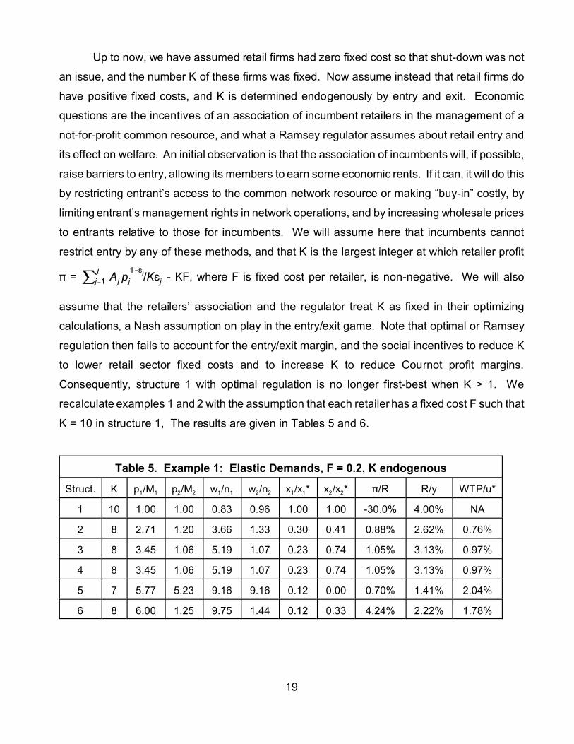
Up to now, we have assumed retail firms had zero fixed cost so that shut-down was not

an issue, and the number K of these firms was fixed. Now assume instead that retail firms do

have positive fixed costs, and K is determined endogenously by entry and exit. Economic

questions are the incentives of an association of incumbent retailers in the management of a

not-for-profit common resource, and what a Ramsey regulator assumes about retail entry and

its effect on welfare. An initial observation is that the association of incumbents will, if possible,

raise barriers to entry, allowing its members to earn some economic rents. If it can, it will do this

by restricting entrant’s access to the common network resource or making “buy-in” costly, by

limiting entrant’s management rights in network operations, and by increasing wholesale prices

to entrants relative to those for incumbents. We will assume here that incumbents cannot

restrict entry by any of these methods, and that K is the largest integer at which retailer profit

B = - KF, where F is fixed cost per retailer, is non-negative. We will also

assume that the retailers’ association and the regulator treat K as fixed in their optimizing

calculations, a Nash assumption on play in the entry/exit game. Note that optimal or Ramsey

regulation then fails to account for the entry/exit margin, and the social incentives to reduce K

to lower retail sector fixed costs and to increase K to reduce Cournot profit margins.

Consequently, structure 1 with optimal regulation is no longer first-best when K > 1. We

recalculate examples 1 and 2 with the assumption that each retailer has a fixed cost F such that

K = 10 in structure 1, The results are given in Tables 5 and 6.

Table 5. Example 1: Elastic Demands, F = 0.2, K endogenous

Struct. K p1/M1 p2/M2 w1/n1 w2/n2 x1/x1* x2/x2* B/R R/y WTP/u*

1 10 1.00 1.00 0.83 0.96 1.00 1.00 -30.0% 4.00% NA

2 8 2.71 1.20 3.66 1.33 0.30 0.41 0.88% 2.62% 0.76%

3 8 3.45 1.06 5.19 1.07 0.23 0.74 1.05% 3.13% 0.97%

4 8 3.45 1.06 5.19 1.07 0.23 0.74 1.05% 3.13% 0.97%

5 7 5.77 5.23 9.16 9.16 0.12 0.00 0.70% 1.41% 2.04%

6 8 6.00 1.25 9.75 1.44 0.12 0.33 4.24% 2.22% 1.78%

20

Table 6. Example 2: One Demand Inelastic, F = 1.0, K endogenous

Struct. K p1/M1 p2/M2 w1/n1 w2/n2 x1/x1* x2/x2* B/R R/y WTP/u*

1 10 1.00 1.00 0.00 0.90 1.00 1.00 -51.1% 3.92% NA

2 14 2.46 1.10 2.17 1.08 0.84 0.83 2.49% 5.76% 0.62%

3 20 6.14 0.51 8.21 0.00 0.70 3.80 3.64% 12.1% 3.88%

4 14 2.53 1.04 2.26 1.00 0.83 0.93 2.76% 5.96% 0.62%

5 22 2.81 1.48 1.81 1.81 0.81 0.46 1.41% 5.73% 1.71%

Note that for structure 1, B/R is the ratio of total industry profits, including the network, to

industry revenue; the profits of the retail sector are non-negative and the regulator makes no

lump sum transfers to this sector. When K is endogenously determined by entry and exit,

industry self-regulation tends to decrease K when demands are elastic, and increase K when

a demand is inelastic. However, the welfare consequences of alternative structures are very

similar, with structure 4 nearly as good as Ramsey pricing in all circumstances, and structures

3 and 5 substantially worse in some circumstances.

These examples serve to illustrate the usefulness of the Gorman representative

consumer assumption for welfare analysis, and estimation of the benefits (which must be

weighed against the costs) of various levels of intervention in industrial structure, e.g., full

Ramsey regulation of a common network entity, or a legal requirement that wholesale prices at

least cover network marginal costs. From these examples, we conclude that it is possible to

achieve a reasonable welfare outcome under industry self-regulation of a common network

resource. If the goods sold by the industry have elastic demands, then network operation as

a non-for-profit enterprise with non-negative wholesale prices is sufficient without regulatory

supervision. However, if some of the goods have inelastic demands, then it is possible for the

retailer’s association to manipulate wholesale prices within the network’s budget constraint to

substantially increase retail profits, with a substantial deadweight loss. This can be avoided by

imposing a “no cross-subsidization” regulatory constraint that all wholesale prices cover marginal

costs. An alternative form of supervision, requiring uniform wholesale markup rates, generally

entails larger deadweight losses for consumers.

21Market prices p are assumed independent of location in this formulation, but this is not essential,

and can be generalized even within the current notation by letting the location determine the subset of

market goods that are feasible to consume.

21

5. Consumers in Space

Welfare analysis using the Gorman polar preference field can handle heterogeneity in

tastes, income, and non-market environments. It does so most easily when Engle curves are

affine linear and parallel for different D and z, and the distribution of z is exogenous and hence

independent of income, so that market demands are consistent with the preferences of a

representative consumer. Even without the representative consumer characterization, when

individual Gorman polar demand functions can be recovered and are sufficient to identify all the

effects of non-market goods on utility, it remains easy to compute individual WTP, and from this

deduce the distribution of WTP in the population, or moments or quantiles of this distribution.

With the reinterpretation that follows, this preference field also facilitates analysis of consumer

choice in space.

Consumers may face location or address choices in hedonic or physical space, and may

be heterogeneous in their endowed tastes or initial location. The indirect utility of location t in

a choice set T may be written in general as

(31) u = V(p,y-r(t),z(t),t,D),

where r(t) is the cost of location t and z(t) describes the non-market environment at this

location.21 The function (31) can be interpreted as the maximum utility obtainable in the market,

conditioned on location t. This function inverts to an expenditure function

(32) y - r(t) = M(p,u,z(t),D).

The consumer will choose a location to maximize (31),

(33) u = V*(p,r,y,z,D) / maxt0T V(p,y-r(t),z(t),t,D),

22The properties of ind irect utility functions (quasi-convex and homogeneous of degree zero in

(p,r,y), increasing in y, non-increasing in p,r) are preserved by the operation of maximization over a set T.

22

where r, z denote the cost and environment functions on T.22 The associated expenditure

function is

(34) y = M*(p,r,u,z,D) / mint0T {r(t) + M(p,u,z(t),t,D)}.

Combining (33) and (34), a money-metric utility function for the consumer in space is

(35) u = :*(pN,rN,zN;p,r,y,z,D) = mint0T maxs0T :st(pN,rN,zN;p,r,y,z,D)

where

(36) :st(pN,rN,zN;p,r,y,z,D) = r(t) + M(pN,V(p,y-r(s),z(s),s,D),zN(t),t,D)

is the s-location, t-metric money-metric utility.

Equation (32), or equivalently, (36), with D interpreted as a random effect that varies

across (or within) members of the population, is a random utility maximization (RUM) model; see

McFadden (1973, 1981). It is simplest to think of T as a finite set, giving a discrete choice

problem, but in general we will require only that T be a compact subset of a finite-dimensional

address space, that z be contained in a compact space of functions from T into Z, and that r be

a point in the Banach space B(T,T) of uniform limits of real-valued linear combinations of

characteristic functions on the Borel F-field T of T. Let *(@;p,r,y,z,D) be a probability measure

on T, defined when the set of maximands in (33) is non-empty, whose support is contained in

the set of maximands; it is an indicator for choice when there is a unique maximand, and is

otherwise interpreted as the random device used by the consumer to break ties. Note that Roy’s

identity holds when there is a unique maximand in t, so that

(37) *(t;p,r,y,z,D) = - Lr(t)V*(p,r,y,z,D) /LyV*(p,r,y,z,D).

23Technical machinery is needed to define (38) when T is infinite, but intuitively it can be

characterized as the probability limit of an average of the integrand over trajectories g drawn by simulation

from the distribution Qg(g|0).

24Defining g*(t) = V(p,y-r(t),z(t),t,0,g(t)) - V(p,y-r(t),z(t),t,0,0) and renaming g*(t) as g(t) gives the

form (40) without loss of generality, but the requirement that this disturbance have a specified distribution

Qg(g|0) independent of the other variables in the problem is a substantive restriction on the preference

field.

23

Now consider a population of consumers with heterogeneous tastes D composed of

components g(t) that vary with t, and components 0 that do not, so that D = (0,g). Suppose

income y and the non-market profile z are statistically independent of g, given 0 This

assumption will hold, for example, if 0 is a sufficient statistic for the mechanism that assigns y

and z. Then choice probabilities in the population, conditioned on 0, y, and z, satisfy

(38) PT(A|p,r,y,z,0) = *(A;p,r,y,z,0,g)Qg(dg|0)

for A 0 T. The integral in (38) can be non-trivial to calculate even when T is finite.23 Thus, it is

useful to consider cases where (38) has a tractable form. A useful simplification is to consider

conditional indirect utility functions of the additively separable form

(39) u = V(p,y-r(t),z(t),t,0,g(t)) = V1(p,y-r(t),z(t),t,0) + g(t),

where V1 is independent of g(t) and g has a distribution Qg(g|0) that gives a tractable integral in

(38).24 An alternative simplification that is very useful is to assume that preferences have a

Gorman polar form,

(40) u = V(p,y-r(t),z(t),t,0,g(t)) = [y - r(t) - b(p,z(t),t,0,g(t))]/a(p,z(t),t,0),

where a(p,z(t),t,0) and b(p,z(t),t,0,g(t)) are linear homogeneous and concave in p. A further

assumption, that the function a(p,z(t),t,0) is independent of any variables that vary with location,

a(p,0); induces a “parallel Engle curves” property across locations. The form (40) with a(p,0)

independent of location is also termed an Additive Income Random Utility Maximization (AIRUM)

model. This leads to a locationally representative consumer whose demands at various

25This specification is intrinsically finite . However, it is possible, using the m ethods of Dagsvik

(1994,1995), to construct extreme value processes on a continuum, and use the properties in Lemm a 2

below to build up generalized extreme value processes that generate closed form choice probabilities on a

continuum.

24

locations are the choice probabilities. Note that in general we do not require in (40) that the

taste disturbance g(t) be additive and linear. There is a common model nested within (39) and

(40): Suppose a(p,z(t),t,0) in (40) is linear in p, and the function b has the additively separable

form b(p,z(t),t,0,g(t)) = b1(p,z(t),t,0) + a(p,z(t),t,0)g(t). Then indirect utility satisfies

(41) u = V(p,y-r(t),z(t),t,0,g(t)) = [y - r(t) - b1(p,z(t),t,0)]/a(p,z(t),t,0) + g(t).

We will first analyze spatial demand models in what we will term the Generalized Extreme

Value case, based on (39) and what is called the GEV family of distributions for the

disturbances. After this, we analyze what we will term the locationally representative Gorman

consumer case, based on(40) and a locationally parallel Engle curves restriction.

Generalized Extreme Value Case

Consider (39) with T = {t1,...,tJ} finite, and assume that the additively separable taste

disturbance g(t) has a Generalized Extreme Value (GEV) distribution. To define this distribution,

first define a GEV generating function H(w1,...,wJ|0): a non-negative linear homogeneous

function of non-negative (w1,...,wJ) with mixed partials that satisfy an alternating sign condition

(-1)jMjH/Mw1...Mwj # 0 for j = 1,...,J. Term such a function S-proper for a subset S of T if H(1j|0)

> 0 for all j 0 S, and H(1T\S|0) = 0. A GEV distribution is of the form

(42) Qg(g|0) = exp(-H(exp(-g1),...,exp(-gJ)|0),

where H is a T-proper GEV generating function.25 As a notational shorthand, let uj = u(tj), vj =

V1(p,y-r(tj),z(tj),tj,0), and gj = g(tj). Let ( = 0.5772 denote Euler's constant, and ' denote the

gamma function. A standardized univariate Extreme Value Type 1 (EV1) distribution function

has the form exp(-exp(-g)). The following result, from McFadden (1978) and Beirlaire, Bolduc,

and McFadden (2003), shows that GEV distributions yield closed-form choice probabilities:

25

Theorem 1. If H(w1,...,wJ |0) is a T-proper GEV generating function, then a random

vector (u1,...,uJ) satisfying (39), with g satisfying (42), has the properties

A. The uj for j = 1,...,J are EV1 with common variance B2/6, means vj + log H(1j |0) + (,

and moment generating functions exp(>vj)H(1j)>'(1->).

B. u0 = maxi=1,...,J ui is EV1 with variance B2/6, mean log H(exp(v1),...,exp(vJ)) + (, and

moment generating function H(exp(v1),...,exp(vJ))>'(1->).

C. Letting Hj(w1,...,wJ|0) = MH(w1,...,wJ|0)/Mwj, the probability Pj that j = argmaxi0T ui

satisfies

(43) Pj = PT(tj|p,r,y,z,0) = .

The linear function H(w) = w1 + ... + wJ is a GEV generating function; the vector

(g1,...,gJ) given by (42) for this H has independent extreme value distributed components.

The choice probabilities (43) then have a multinomial logit (MNL) form,

(44) Pj = exp(vj)/'i0T exp(vi).

The next result gives operations on GEV generating functions that can be applied recursively

to generate additional GEV generating functions.

Lemma 2. The family of GEV generating functions is closed under the operations:

A. If H(w1,...,wJ |0) is a S-proper GEV generating function, S f T, then

H("1w1,...,"JwJ |0) for "1,...,"J $ 0 and B = {j0S|"j > 0} is a B-proper GEV

generating function..

B. If H(w1,...,wJ |0) is an A-proper GEV generating function and F > 1, then

H(w1F,...,wJ

F |0)1/F is an A-proper GEV generating function for A f T.

26

C. If HA(w1,...,wJ |0) and HB(w1,...,wJ |0) are, respectively, A-proper and B-proper

GEV generating functions, where A, B fT are not necessarily disjoint, then

HA(w1,...,wJ |0) + HB(w1,...,wJ |0) is a AcB-proper GEV generating function.

.

McFadden and Train (2000) show for discrete choice that any regular random utility

can be approximated as a 0-mixture of GEV-distributed utilities, and thus market-level

discrete choice probabilities are approximately 0-mixtures of (44). Note that choice

probabilities based on Theorem 1 may depend on income, and thus capture choice behavior

that varies with income.

Locationally Representative Gorman Consumer Case

A preference restriction leading to tractable choice probabilities is the Gorman polar

form (40) with a(p,0) independent of location. The expectation with respect to the

distribution Qg(g|0) of the maximum of these conditional utility functions over location is a

representative consumer utility function that is again of Gorman polar form,

(45) u = V*(p,r,y,z,0) / maxt0T [y - r(t) - b(p,z(t),t,0,g(t))]Qg(dg|0)/a(p,0)

= y/a(p,0) + G(p,r,z,0),

where

(46) G(p,r,z,0) = maxt0T [ - r(t)/a(p,0) - b(p,z(t),t,0,g(t))]Qg(dg|0)/a(p,0).

The demands obtained from (45) by applying Roy’s identity to the price vector r are the

choice probabilities (38): PT(t|p,r,y,z,0) = -a(p,0)MG(p,r,z,0)/Mr(t). The function G(p,r,z,0) in

(46) is termed a social surplus function; it necessarily has the properties

27

(i) G is homogeneous of degree zero, convex, and non-increasing in (p,r),

(ii) For any scalar 2, G(p,r+2,z,0) = G(p,r,z,0) - 2,

(iii) All the mixed partials of G with respect to r exist and are non-positive.

These properties are also sufficient for a function G to satisfy the construction (46) for some

distribution Qg(g|0). The essential elements of this characterization are due to Williams

(1977) and Daly and Zachery (1978); the result is proved in McFadden (1981), who notes its

close relation to the aggregation properties of the Gorman polar form:

Theorem 3 [Williams-Daly-Zachery]. Consider the field of additive-income random

utility models (AIRUM) of the form (40) with a(p,z(t),t,0) and b(p,z(t),t,0,g(t)) positive, non-

decreasing, linear homogeneous, and concave in p, The mapping (45) from AIRUM

preferences is onto the class of social surplus functions satisfying (i)-(iii).

In the case of the preference field (41) that is common to both the Generalized

Extreme Value and the Locationally Representative Gorman Consumer cases, both

Theorem 1 and Theorem 2 apply, and establish that

(47) G(p,r,z,0) = log H(exp(-[r1-b1(p,z1,t1,0]/a(p,0)),...,exp(-[rJ-b1(p,zJ,tJ,0]/a(p,0))) + (,

with choice probabilities satisfying (43) with vj = -[rj-bj(p,zj,tj,0]/a(p,0). In this combined case,

the choice probabilities are independent of income. When this case is realistic for

applications, it facilitates welfare analysis by eliminating income effects.

6. Consumer Welfare at the Extensive Margin

The welfare analysis problem for the consumer in space can be stated as that of

determining mean WTP or WTA, or quantiles of the distributions of WTP or WTA, for a

change from (pN,rN,yN,zN) to (pO,rO,yO,zO), based on individual or market-level observations on

choice behavior. McFadden (1999) analyzes the problem of estimating or bounding WTP

and WTA for this problem; the following summary is most easily interpreted when T is finite,

but finiteness is not essential. For any s,t 0 T, define Cst as the net compensating variation

28

(i.e., net reduction in final income) that makes a consumer indifferent to location s before the

change and location t after the change; i.e.,

(48) Cst = :st(pO,rO,zO;pO,rO,yO,zO,D) - :st(pO,rO,zO;pN,rN,yN,zN,D)

= yO - rO(t) - M(pO,V(pN,yN-rN(s),zN(s),s,D),zO(t),t,0,g).

Define C* to be the compensating variation that equates maximum utility over T before and

after the change. Then

(49) C* = yO - :*(pO,rO,zO;pN,rN,yN,zN,D) = yO - mint0T maxs0T :st(pN,rN,zN;p,r,y,z,D)

= maxt0T mins0T Cst.

Hence, the optimal locations sN before the change and tO after the change satisfy

(50) CsNsN # C* # CtOtO.

Define Bst to be the event that s is the optimal location before the change and t is the optimal

location after the change, and define Bs@ = ^t0TBst and B@t = ^s0TBst. Let PN(s) denote the

uncompensated location choice probability before the change, and PO*(t) denote the choice

probability after the change when compensation C* is paid, from (50). In general, the

quantities CsNsN, C*, and CtOtO all depend on g. Mean WTP, conditioned on (0,

pN,yN,rN,zN,pO,rO,yO,zO), satisfies the bounds

(51) E(Css|Bs@)PN(ds) # WTP # E(Css|B@s)PO*(ds),

where E(Css|Bs@) denotes conditional expectation given the event Bs@. A completely

analogous development in terms of constant-location equivalent variations Ess yields similar

inequalities,

(52) E(Ess|Bs@)PN*(ds) # WTA # E(Ess|B@s)PO(ds),

29

where PO denotes the uncompensated location choice probability after the change, PN*

denotes the choice probability before the change when compensation equal to the overall

equivalent variation E* is given, and the events Bst and their unions are now defined with

equivalent rather than compensating adjustments.

A substantial simplification of (51) and (52) occurs when preferences have the

specification (39), with additively separable taste disturbance g(t), as in this case the

constant-location compensating and equivalent variations do not depend on g and one has

E(Css|Bs@) = Css and E(Ess|B@s) = Ess. Since the left-hand inequality in (51) and the right-hand

inequality in (52) do not require knowing the overall compensating and equivalent variations

C* and E*, these bounds are relatively straightforward to compute. Then, (51) and (52) may

provide easy bounds that are sufficiently tight to guide policy without recovering individual

WTP and WTA. Note that the terms in these inequalities can be integrated with respect to

the distributions M(z|0,y,.)'(y|0,Y)Q0(0) to obtain bounds on the overall population mean

WTP and WTA. Alternately, lower and upper bounds on the distribution of WTP and WTA

can be obtained by noting that

(53) 1(Css $ ")PN(ds) # Prob( " # WTP # $) # 1(Css # $)PO*(ds)

and

(54) 1(Ess $ ")PN*(ds) # Prob( " # WTA # $) # 1(Ess # $)PO(ds).

Thus, a project is desirable by a mean benefit-cost criterion if 0 # CssPN(ds) , and

undesirable if 0 $ EssPO(ds), while this project is desirable by a median voter criterion if ,

0.5 # 1(Css $ 0)PN(ds) and undesirable if 0.5 $ 1(Ess # $)PO(ds).

When T is finite and preferences have the form (39) with generalized extreme value

distributed additive taste disturbances, Theorem 1 gives closed forms for the choice

30

probabilities in (51) and (52), and also implies a “certainty equivalent” compensating variation

C# satisfying

(55) ,

where vjN = V1(pN,yN-rN(tj),zN(tj),tj,0) and vjO* = V1(pO,yO-rO(tj)-C#,zO(tj),tj,0). The bounds (50)

hold for C# as well as for C*, but in general these quantities are not equal, and C# is a biased

estimate of C*. The exception where C# equals C* occurs when V1 is linear in y, a case that

corresponds to the preference field (40).

Next consider preferences that have the Gorman polar form (41). Then the constant-

location compensating and equivalent variations have explicit forms,

(56) Css = a(pO,zO(s),s,0) ,

(57) Ess = a(pN,zN(s),s,0) .

These provide relatively convenient bounds in (51) or (52). However, the greatest

simplification comes when a(p,z(s),s,0) is independent of location. Then, location minimizes

[r(t) + b(p,z(t),t,0)]/a(p,0) - g(t), independently of y, and the exact compensating variation has

the explicit form

(56) C* = .

31

When the set T is finite, and the vector of additive taste disturbances g has a GEV

distribution with GEV generating function H, then from Theorem 1,

(59) E C* = ,

where vjO = [yO - rO(tj) - b(pO,zO(tj),tj,0)]/a(pO,0) and vjN = [yN - rN(tj) - b(pN,zN(tj),tj,0)]/a(pN,0). This

formula can be mixed with respect to the distribution '(y|0,Y)Q0(0) to give mean

compensating variation for the population, and a project is desirable by this criterion if and

only if

(60) 0 < .

This is the same criterion that one would obtain from a '(y|0,Y)Q0(0) population mixture of

locationally representative Gorman polar consumers with indirect utility functions

(62) u = ,

where vj* =[ - r(tj) - b(p,z(tj),tj,0)]/a(p,0).

7. An Application: Consumer Harm from Proximity to a Hazardous Waste Site

Suppose consumers choose residential location to maximize utility, taking into

account the price and hedonic attributes of houses in the market. Heterogeneity in

consumer tastes will lead them to sort themselves out over locations, with the prices at

various locations adjusting to clear the market. Suppose it is revealed that a neighborhood

is in the proximity of a hazardous waste site that has produced groundwater contamination.

32

A new equilibrium will be reached, with housing prices adjusting and consumers relocating in

response to concerns about the contamination. The economic questions are WTP or WTA

for remediation of the contamination, and the conditions under which these welfare

measures can be identified from market observations. The analysis that follows could also

be applied to determine the welfare effects of an urban transportation system improvement,

such as the addition of a link to the transportation network, that has spatially distributed

effects. The translation of language for this application is left to the reader.

Current practice in natural resource damage assessment is to use one of three

measurement approaches:

(1) The hedonic price method (HPM) in which housing prices are regressed on

dwelling, neighborhood, and overall market attributes, and variables that capture

permanent neighborhood effects, background time effects, and interaction effects that

are intended to capture the impact of the contamination announcement on the

affected neighborhood.

(2) The travel cost method (TCM) in which location decisions of individual consumers

are estimated as discrete choice functions of housing and neighborhood attributes,

dwelling prices, and indicators for neighborhood, time, and interaction effects.

(3) The stated preference method (SPM) in which WTP for changes in environmental

conditions is elicited in experiments that offer hypothetical market choices that include

environmental goods that in reality do not have markets.

Initial questions are how these measures are related to WTP and WTA, and what theoretical

restrictions and data circumstances will allow us to estimate or bound the impact of the

revealed contamination on consumer welfare.

I will not be concerned in this paper with SPM and TCM. Clearly, SPM experimental

methods can recover all aspects of preferences, provided the hypothetical setting and

incentives can be structured to elicit responses consistent with preferences and behavior in

the real world. The challenge is to define such experiments. The TCM can recover all

features of utility that vary with location. If for example consumers have preferences of the

Gorman polar form (41) with additive GEV taste disturbances g(tj), then exact expected

compensating variation is given by (59), which depends on the expression vj = [y - r(tj) -

b(p,z(tj),tj,0)]/a(p,0) evaluated before and after a change. Components of this formula that

do not vary with t, but do vary with the change, cannot be identified by the TCM, but may be

33

identified by this method augmented with estimates of the market demand for the

commodities with price vector p. Typically in applications, the environmental change is

assumed to leave invariant variables that do not vary with t, so that identification of expected

WTP is achieved by TCM. Separability assumptions on the preference field may be

important in achieving identification in the presence of effects that do not depend on t.

I turn now to the hedonic price method. The basic idea of this method is that if two

properties, one in a “treatment” area affected by the environmental hazard, the other in an

unaffected “control” area, are identical in all other respects, then the difference in their

market prices reflects the value consumers place on the hazard. The controls might include

properties in a nearby neighborhood that are not exposed to the hazard, or properties in the

affected neighborhood at a time when the hazard is absent, or both. The “value” measured

by the HPM is a pecuniary loss, which is not in general the same as the monetized loss in

utility, or WTP, of residents in the affected neighborhood. We ask how the two differ, and

when the second can be recovered from information on the first.

If properties and neighborhoods differ in their attributes over location or time, then

these differences confound observation of the effect of the hazard. However, it is possible to

control and correct for the effect of observed attributes by use of an appropriately specified

hedonic regression. As a practical matter, successful isolation of the effects of the hazard

from possible confounders requires accurate measurement of attributes, search for the

appropriate functional form and the variable transformations and interactions it requires, and

careful attention to experimental design to identify and isolate significant confounders. To

control possible confoundment from both persistent neighborhood effects and time variation

in the overall market, current “best practice” in environmental economics is to use a two-way

experimental design, with observations in control neighborhoods unaffected by the hazard,

as well as the affected neighborhood, both during the period when the hazard is present and

before it appeared. These observations are analyzed in a regression model

(63) ywnt = "n + (t + *w + xwnt$ + gwnt,

where

n neighborhood (n = 1 for treated, n = 0 for controls)

34

t time (t = 0 before hazard, t = 1 during hazard)

w hazard indicator (w = n@t)

y log sales price

x measured property and neighborhood attributes

, disturbance

In this model, "n is a persistent neighborhood effect, (t is an overall time effect, and *w is

interpreted as the average percent diminution in values of the affected properties attributable

to the hazard. The reason for introducing the apparently superfluous hazard indicator w = n@t

is that later we will consider the counterfactual w / 0, and the counterfactual values x011 and

y011. Normalizations "0 = (0 = *0 = 0 are imposed for identification.

In the terminology of the analysis of treatment effects, the mean effect of the hazard

on properties in the affected neighborhood is called the average effect of treatment on the

treated, given x, and is defined as

(64) E{TT|x} = E{y111|x} - E{y011|x},

where y111 is log sales price in the factual case that treatment (exposure to the hazard, or w =

1) occurs in the affected neighborhood n = 1 at time t = 1, and y011 is the (unobserved) log

sales price in the counterfactual case that there is no hazard (w = 0) at n = t = 1. Under

some assumptions, the counterfactual conditional expectation can be expressed as a linear

combination of conditional expectations that can be estimated from observations,

(65) E{y011|x} = E{y010|x} + E{y010|x} - E{y000|x}.

Substituting (65) into (64) gives a difference-in-difference (DID) formula for the conditional

average effect of treatment on the treated,

(66) E(TT|x) = E(y111|x) - E(y010|x) - E(y001|x) + E(y000|x);

35

see Heckman and Robb (1986). If in particular, the determination of prices is described by

the hedonic regression model (63), and the disturbance in this equation satisfies the critical

assumption E(gwnt|w=n@t,n,t,x) = 0, then one has

(67) *1 = E(TT|x).

If the regression model (64) satisfies Gauss-Markov conditions, then the OLS estimator of *1

is an estimate of the average effect of treatment on the treated. The question then is what

economic assumptions imply Gauss-Markov conditions, or other conditions under which

alternative estimation methods yield consistent estimates of *1.

The additive linear specification of the regression (63) is apparently very restrictive,

although by redefinition of x to include suitable transformations and interactions, and

generalization of g to allow conditional heteroskedasticity, it can be treated as a method of

sieves approximation to a more general model. However, an approach introduced by

Matzkin (2002) provides a more direct generalization of (66), and allows estimation of

generalized moments of TT other than the conditional mean, an important consideration for

policy applications. Describe the determination of y by a model

(68) y = h(w,n,t,x,g)

in which no linearity or additivity conditions are imposed. Let Fnt(y|x) denote the conditional

distribution of y, given n, t, and x (with w = n@t), Tnt(x) denote the density of x given n,t, and y

= Gnt(q|x) denote the conditional quantile function; i.e.,

(69) Gnt(q|x) = sup{y|Fnt(y|x) < q)}.

The effect of treatment on the treated (TT) is defined, consistently with (64), is

(70) TT(x,,) = h(1,1,1,x,,) - h(0,1,1,x,,),

the change in the outcome y at n = t = 1 when w changes from the counterfactual value of 0

to the factual value of 1, and x and , are unchanged. The following result adapted from

36

Matzkin (2002) provides conditions under which the conditional expectation E{A(TT,x)|x} of

any summable functional A(TT,x) can be identified and estimated.

Theorem 4. Suppose the model (68) is continuous in (x,g), with x of dimension k, and

satisfies

(i) h is strictly increasing in g,

(ii) g is statistically independent of (w,n,t,x),

(iii) h(0,1,1,x,g) - h(0,1,0,x,g) = h(0,0,1,x,g) - h(0,0,0,x,g); e.g., the effect of time on the

treated in the counterfactual that they are untreated is the same as the actual effect of

time on the untreated.

(iv) The densities Tnt are positive at x.

Suppose TT satisfies (70), and A(c,x) is a measurable function of its arguments. Letting q

denote a uniform random variable on (0,1), TT can be written

(71) TT = DID(q,x) = G11(q|x) - G10(q|x) - G01(q,x) + G00(q,x),

and if E{A(TT,x)|x} exists, then

(72) E{A(TT,x)|x}= A(DID(q,x),x)dq.

Proof: Substituting (iii) into (70), one has

(73) TT(x,,) = h(1,1,1,x,,) - h(0,0,1,x,,) - h(0,1,0,x,,) + h(0,0,0,x,,).

In sub-population 11, , has a CDF q = '(,), and inverse function , = '-1(q). By (ii), it has the

same distribution for the sub-populations 10, 01, 00. By (i), the conditional quantile functions

Gnt(q|x) in each of the sub-populations satisfy Gnt(q|x) = h(n@t,n,t,x,'-1(q)). Then, substituting

, = '-1(q) in (73), one has the result that TT, written as a function of x and a uniform random

variable q, has the form (71). Condition (iv) assures that TT is well-defined at x. Note that

DID is not in general monotone in q. Finally, given A(c,x), one can substitute (71) to obtain

(73). ~

37

When A is linear, the expectation (72) will coincide with (66). More generally, (72) can

be used as a basis for estimators of non-linear functions of TT, such as step functions that

give the conditional CDF of TT. The next result gives a convenient estimator for (72) that is

also adapted from Matzkin (2002).

Theorem 5. Suppose i.i.d. observations (yi,ni,ti,xi), for i = 1,...,N, and assume the

observations are ordered so that y1 # ... # yN. Let Nnt = 1(ni=n)@1(ti=t) denote the

number of observations in sub-population nt. Let R denote a continuous k-dimensional

probability density that is positive in a neighborhood of zero, 7 denote a one-dimensional

CDF with the property that 7(z) - ½ has the same sign as z, and FN denote a window width

that satisfies FN 6 0 and NFNk+1 6 4. Then the kernel estimator

(74) Fnt#(y|x) = (Nnt FN

k+1)-1 1(ni=n)@1(ti=t)R((x-xi)/8N)7((y-yi)/FN)

satisfies Fnt#(y|x) 6p Fnt(y|x) at each x for which Tnt(x) > 0, and the conditional quantile

estimator Gnt#(q|x) = max{y|Fnt

#(y|x)<q} satisfies Gnt#(q|x) 6p Gnt(q|x).

Corollary 6. Suppose the hypotheses of Theorem 5, with 7(z) = 1(z$0). Define

(75) Qnt#(y|x) = (Nnt8N

k+1)-1 1(ni=n)@1(ti=t)R((x-xi)/8N)@1(yi#y).

Then,

(76) Gnt#(q|x) = max{yi|Qnt

#(yi|x) < q}.

38

Proof: The estimator (74) from Theorem 5, with 7(z) = 1(z$0), is

Fnt#(y|x) = (Nnt8N

k+1)-1 1(ni=n)@1(ti=t)R((x-xi)/8N)1(yi#y) /Qnt#(y|x).

Then (76) follows from the inversion formula for the quantile function and the fact that

Qnt#(y|x) is piecewise constant in y with knots at the observations yi. ~

The convenience of(76) is that it is unnecessary to invert q = Fnt#(y|x) numerically.

The estimator (76) is piecewise constant and right-continuous, with jumps at the knots

Qnt#(yi|x) for i = 1,...,N where ni = n and ti = t. A continuous modification of (76) could be

constructed by linear interpolation between the adjacent knots. Using the estimators

Gnt#(q|x) from Theorem 5 or Corollary 6 yields a computationally convenient consistent

estimator of E{A(TT,x)|x}.

Corollary 7. Suppose the hypotheses of Theorems 4 and 5. Define

(77) DID#(q,x) = G11#(q|x) - G10

#(q|x) - G01#(q,x) + G00

#(q,x).

Define an collection of points qj for j = 0,...,4N+1, with q0 = 0, q4N+1 = 1, and the remaining

points given by Q11#(yi|x), Q10

#(yi|x), Q01#(yi|x), and Q00

#(yi|x) for i = 1,...,N, ordered so that q0 #

q1 # ... # q4N+1, . Then,

(78) E#{A(TT,x)|x} = A(DID#(qj,x),x)(qj+1 - qj-1)/2

satisfies E#{A(TT,x)|x} 6p E{A(TT,x)|x}.

With additional assumptions on the smoothness properties of the distributions Fnt(y|x),

densities Tnt, the function A(z,x), and the kernels used in constructing the estimators in

Theorem 5 and its corollaries, one can establish optimal rates for the window width 8N, and

establish asymptotic normality for the estimators (76)-(78).

39

The most serious questions about application of Theorems 4 and 5 to estimate

pecuniary losses from an environmental injury are the validity of the assumption that the

effect of time on the treated if left untreated is the same as the effect of time on the

untreated, and the assumption that the distribution of the disturbance , does not depend on

n, t, and x. In the next section of this paper, we will examine the structure of hedonic

equilibrium and its implications for the properties of the treated versus the untreated, and the

properties of ,. At this point, it should be noted that , summarizes the effects of

unobservables that are primitive to the economy, including consumer preferences,

unmeasured attributes of properties and neighborhoods, and imperfections in the functional

specification of (68). Further, selection effects, in which consumer choice of neighborhood

n induces a dependence of the distribution of , on n, and feedback effects, in which the

causal link from n, t, and x is confounded by a reverse causal link from y to x, will make the

DID estimator of TT inconsistent. Methods for dealing with selection and feedback effects

can be found in Heckman and Robb (1986) and Altonji and Matzkin (2003).

We next explore in a very simple general equilibrium economy the validity of the fairly

conventional "difference-in-difference" or "random effects hedonic regression" method for

resource valuation. We show in two simple examples that this method does accurately

measure the pecuniary loss from an environmental injury, but that it does not in general

estimate WTP. In the first example, there is insufficient information from the market to

identify WTP, or in other terms, to identify the distribution of preferences, because of

bunching of consumers with heterogeneous infra-marginal preferences.. In the second

example, where all consumers are at an active margin, it is possible at least in some cases

to identify preferences and recover WTP from a modified measure of loss that does not in

general coincide with the pecuniary loss. These examples do not construct a general

equilibrium economy where the “difference-in-difference” fails to estimate the pecuniary loss

accurately, but it is clear that one could do so, since this method removes confounding

effects only under a special hypothesis, and it is simple to see that general equilibrium

effects can easily violate this hypothesis.

Example 1

Consider an isolated city that contains two neighborhoods, n = 0 and n = 1. We will

deal with two time periods, t = 0 and t = 1. The city contains N households, indexed i =

40

1,...,N, with N large. Every household is endowed with an amount y of a composite good,

which we will call "income", received each time period. The price of the composite good is

normalized to one. In addition, there is one consumer, household 0, who lives outside the

city and is endowed with a stock of N1 identical housing units located in neighborhood n = 1,

fixed in t, and a reversible constant returns technology that can transform between housing

units in n = 0 and income at a marginal cost rt in period t. Let 2 = N1/N and assume 0 < 2 <

1.

There is a possible environmental hazard, indicated by w = 1 if it is present, and w = 0

otherwise. At t = 0, there is no environmental hazard in either neighborhood, and at t = 1,

the environmental hazard is present in neighborhood n = 1 but not in n = 0. Then w = n"t in

the factual situation. We want to also consider the counterfactual situation with w = 0 at n = t

= 1.

Summarizing, the economy has four commodities in each period: housing units in n =

0 and n = 1, an environmental hazard that may be present at t = 1 in n = 1, and a composite

good. The environmental hazard is not directly priced or controlled by the market.

Measured in units of the composite good, the rental price of a housing unit in state wnt is

denoted rwnt. In the factual situation, households face prices (r000,r010) at t = 0 and prices

(r001,r111) at t = 1. In the counterfactual situation, households face prices (r001,r011) at t = 1.

There are no intertemporal markets, and no way to inventory the composite good.

Assume that the indirect utility of a household i = 1,...,N has the Gorman polar form

(79) u = Max{y-r010-D8,y-r000} + Max{y-r111-D(8+1),y-r001}

in the factual situation, and the form

(80) u = Max{y-r010-D8,I-r000} + Max{y-r011-D8,y-r001}

in the counterfactual situation. The term 8 > 0 is the perceived net disamenity of n = 1

relative to n = 0 when there is no environmental hazard. The parameter D is random, with a

cumulative distribution function Q(D) that has a compact support contained in the

non-negative real line. This reflects heterogeneity in the degree of aversion of households to

the permanent features and the environmental hazard, when present, for n = 1. Despite the

41

linear structure of indirect utility conditioned on neighborhood choice, the presence of this

choice makes the random taste parameter D non-separable. Household 0, the capitalist,

supplies Mt units in n = 0 at time t, and has an indirect utility function for state w

(81) u = y0 + N1(rw11 + r010) + Min(N-N1,M0)r000 - (M0-N+N1)r0

+ Min(N-N1,M1)r001 - (M1- N+N1)r1

The capitalist will supply housing units in n = 0 only if r00t $ r0, and will supply N-N1 units at

p00t = r0.

At t = 0, the consumers with D such that D < (r010-r000)/8 will choose a housing unit in n

= 1. Then, 2 = Q((r010-r000)/8). Then, the equilibrium is r000 = r0 and r010 = r0 + 8D*, where D* /

Q-1(2) is the threshold aversion level for residents of n = 1.

At t = 1, the consumers with D(8+1) < r111-r001 will choose a housing unit in n = 1,

implying 2 = Q((r111-r001)/(8+1)). Then,r001 = r1 and r111 = r1 + (8+1)D*.

There is also a counterfactual equilibrium with w = 0 for t = 1 and n = 1. In this case,

2 = Q((r011-r001)/8). Then, r001 = r1 and r011 = r1 + 8 D*.

Comparing the equilibrium housing allocations, there is no switching between housing

units across the various cases, as n = 1 will always contain the N1 households that are least

adverse to the disamenities of this neighborhood, whether or not the disamenity is amplified

by the environmental hazard.

The sum of the utilities of the N consumers and the capitalist in state w is

(82) Uw = 2Ny + y0 - E(D|D<D*)(28+w)N1.

Then, the compensating variation in income necessary to exactly offset the environmental

hazard is

42

(83) C* = U0 - U1 = N1E(D|D<D*) = N1DQN(D)dD/Q(D*)

= N1D* - N1 Q(D)dD/Q(D*) # N1 D*.

The reason that this is not exactly N1D* is that the infra-marginal households dwelling in n = 1

are less impacted by the additional disamenity of the hazard than the most adverse

household at the extensive household.

The conventional difference-in-difference estimator of injury from the environmental

hazard is

(84) TT = (r111-r010-r001+r000)N1 = N1 D*.

Then, TT overstates C*. Obviously, this happens because TT attributes to every household

in n = 1 the same loss as that of the marginal, most adverse household induced to stay in

the neighborhood. The apparent reason that the usual consumer surplus calculation fails is

precisely that the infra-marginal consumers have no dimension on which they can adjust to a

margin, so their effect is like the effect of unsatisfied secondary market margins in general

equilibrium which make first-order contributions to welfare calculations in second-best

welfare analysis.

At least in the setup above, there is no information contained in the market prices on

the distribution of the infra-marginal D's. Then, one cannot distinguish the extremes in which

all the N1 households in n = 1 have D = D*, or N1 - 1 households have D = 0 and one has D =

D*, so the true equivalent variation could be anything between D* and ND*. Because the

market prices cannot distinguish these cases, they cannot identify the distribution of

consumer preferences. This implies that to have any hope of identifying consumer

preferences from hedonic market data, every consumer must be operating at active margins

with dimensionality at least as great as the dimension of the preference space.

In this example, all housing units were identical, and the environmental hazard

impacted utility in the same dimension as the "permanent" relative disamenity 8 of n = 1. If

households were also choosing among housing units on the basis of observable hedonic

43

attributes x, some components of which might be continuous, could this eliminate bunching

of infra-marginal consumers, restore a margin, and allow identification of preferences? If the

permanent and hazard components of the neighborhood disamenities of n = 1 were

assessed by households in separate dimensions, would this supply the needed margin?

(Letting 8 vary randomly across households would, mechanically, be equivalent to allowing

preference variation in two dimensions.) The next example suggests that under the right

conditions the answer is affirmative.

Example 2

A second example induces an active margin for every household affected by the

environmental hazard. Assume now that within n = 1 at t = 1, housing units are differentiated

by their distance m from the environmental hazard, and the disamenity declines with

distance. Specifically, let G(m) be the CDF of distances from the hazard within n = 1, and

assume that m is scaled so that the support is [0,1]. Assume that the permanent disamenity

in n = 1 also declines with distance m. The price of housing in n = 1 then varies with m; write

rw1tm for the price function. Suppose that the utility of a housing unit at m in n = 1 for a

household with preference parameter D is u = I - rw1tm - D(1-m)(8 + w). The utility of a housing

unit in n = 0 is the same as before. Also, 2 = N1/N is as before the maximum share of

households that can be located in n = 1.

Consider market equilibrium at t in state w. As before, r00t = rt. To avoid dealing with

corner solutions where some dwellings nearest the hazard would be vacant at zero price,

assume that the support of Q(D) is an interval that includes zero. The price function will be

increasing for m > 0. The price function will induce an allocation in which households with

taste parameter D are located at m = Dwt(D). Material balance requires NQ(D) = N1[G(Dwt(D))]

for D # D*, where Q(D*) = N1/N is the proportion of the population occupying units in n = 1.

Utility maximization requires that

(85) rw1tD(D) + D(1-D(D))(8+w) # rw1tm + D(1-m)(8+w).

The first-order condition for this optimization is

(86) 0 = Lmrw1tm - D(8+w),

44

and the second-order condition is

(87) 0 < Lmmrw1tm.

Then, the price function must be increasing and convex. Since at the boundary m = 1, the

disamenities associated with n = 1 are zero, one has the boundary condition rw1t1 = r00t / rt.

Let Q-1(q) be the inverse function solving q = Q(D). Then, the material balance condition

implies D = Q-1(2G(m)) in equilibrium, so that

(88) Lmrw1tm = Q(2G(m))(8+w).

Using the boundary conditions,

(89) rw1tm = max{0,rt - (8+w) Q-1(2G(s))ds}.

The consumers in n = 1 are the N1 least adverse, and they do not switch units with w or t,

remaining in the order of least adverse at m = 0 to most adverse at m = 1. One has D* = Q-

1(2) and Dwt(D) = D(D), as the price change is just sufficient to induce consumers to stay in

place. Computing the equivalent variation for the consumer with preference parameter D,

(90) U0(D) - U1(D) = (I - r011D(D) - D8) - (I - r111D(D) - D(8+1)) = r111D(D) - r011D(D) + D.

Integrated over the consumers in n = 1,

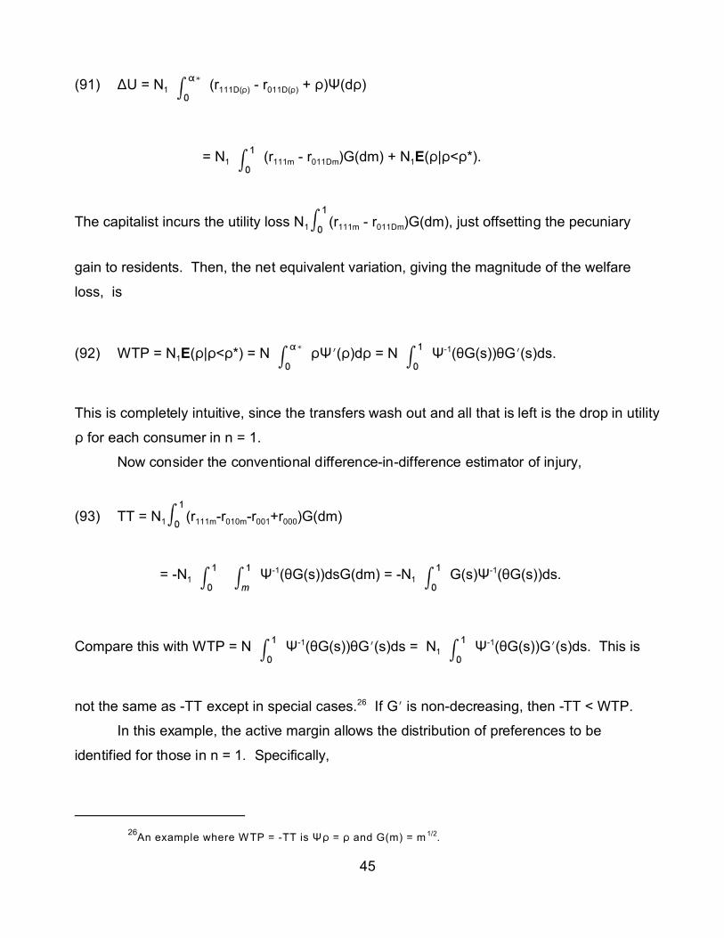
26An example where WTP = -TT is QD = D and G(m) = m 1/2.

45

(91) )U = N1 (r111D(D) - r011D(D) + D)Q(dD)

= N1 (r111m - r011Dm)G(dm) + N1E(D|D<D*).

The capitalist incurs the utility loss N1 (r111m - r011Dm)G(dm), just offsetting the pecuniary

gain to residents. Then, the net equivalent variation, giving the magnitude of the welfare

loss, is

(92) WTP = N1E(D|D<D*) = N DQN(D)dD = N Q-1(2G(s))2GN(s)ds.

This is completely intuitive, since the transfers wash out and all that is left is the drop in utility

D for each consumer in n = 1.

Now consider the conventional difference-in-difference estimator of injury,

(93) TT = N1 (r111m-r010m-r001+r000)G(dm)

= -N1 Q-1(2G(s))dsG(dm) = -N1 G(s)Q-1(2G(s))ds.

Compare this with WTP = N Q-1(2G(s))2GN(s)ds = N1 Q-1(2G(s))GN(s)ds. This is

not the same as -TT except in special cases.26 If GN is non-decreasing, then -TT < WTP.

In this example, the active margin allows the distribution of preferences to be

identified for those in n = 1. Specifically,

46

(94) LmDID(m) = Lm(r111m-r010m-r001+r000) = Lm(r111m-r010m) = Q-1(2G(m))

allows recovery of Q(D) for D < D*. However, in n = 0 where there is no active margin, the

distribution of preferences is not recoverable.

8. Conclusions

The purpose of this paper has been to illustrate the usefulness of Gorman’s polar

form as an ingredient in applied consumer welfare analysis, particularly in problems where

consumer location in space is an endogenous consequence of consumers’ reactions to

changes in the economic environment. Just as a “parallel Engle curves” assumption across

consumers in conventional consumer analysis allows demands to be represented as those

of a single representative consumer, an analogous assumption on Engle curves across

locations for consumers with heterogeneous tastes in space allows spatial choice

probabilities to be represented as those of a “locationally representative” consumer. These

Gorman preferences have sufficient latitude to accommodate quite general patterns of

substitution among commodities, and at least locally reasonable Engle curves, and yet have

sufficient structure to give tractable forms for compensating variations. These in turn permit

one to study the impact on consumer welfare of changes associated with spatially distributed

environmental effects, and to examine the question of whether there is sufficient information

in market observations to identify consumers’ WTP. With examples, we suggest that the key

to identification is the presence of active extensive margins of sufficient dimensionality for

each consumer.

References

Aasness, J.; Bjorn, E.; Skjerpen, T. (2003) “Distribution of Preferences and Measurement Errors in a

Disaggregated Expenditure System,” Econometrics Journal, 6, 373-399.

Altonji, J.; Matzkin, R. (2003) “Cross-section and Panel Data Estimators in Nonseparable Models with

Endogenous Regressors,” Northwestern University Working Paper.

Anderson, G.; Blundell, R. (1983) “Testing Restrictions in a Flexible Dynamic Demand System ,” Review of

Economic Studies, 50, 397-410.

Anderson, S.; De Palma, A.; Thisse; J. (1988) “A Representative Consumer Theory for the Logit Model,”

International Economic Review, 29, 461-466.

Blackorby, C.; Boyce, R.; Russell, R. (1978) “Estimation of Demand Systems Generated by the Gorman Polar

Form : A Generalization of the S-Branch Utility Tree,” Econometrica, 46, 345-363.

Blackorby, C.; Primont, D.; Russell, R. (1978) Duality, Separability, and Functional Structure, North Holland.

Blackorby, C.; Shorrocks, A.; eds. (1995) Separability and Aggregation: Collected Works of W.M. Gorman , Vol.

I,” Oxford Clarendon Press.

47

Boiteaux, M. (1956) “Sur la gestion des monopoles publics astreints à l’équilibre budgétaire,” Econometrica, 24,

22-40.

Brown, D .; Matzkin, R. (1998) “Estimation of Nonparam etric Functions in Simultaneous Equations Models, with

an Application to Consumer Demand,” Cowles Foundation, Yale University, Discussion Paper: 1175.

Browning, M.; Meghir, C. (1991) “The Effects of Male and Female Labor Supply on Commodity Demands,”

Econometrica, 59, 925-951.

Chipman, J. (1990); “Marshall's Consumer's Surplus in Modern Perspective,” in J. W hitaker, ed., Centenary

essays on Alfred Marshall. Royal Economic Society, Cambridge University Press,78-292.

Chipman, J. (1994) ”Hicks ian W elfare Econom ics,” in H. Hagem ann; O. Hamouda, eds. The legacy of Hicks:

His contributions to economic analysis, Routledge, 1994; 96-146.

Chipman, J. (2000) “The New Welfare Economics 1939-1974,” in T. Cowen, ed., Economic Welfare. Elgar

Reference Collection. Critical Ideas in Economics, vol. 3. Cheltenham.

Chipman, J.; Moore, J. (1980) “Compensating Variation, Consumer’s Surplus, and W elfare,” American

Economic Review, 70, 933-348.

Chipman, J.; Moore, J. (1990) “Acceptable Indicators of Welfare Change, Consumer's Surplus Analysis, and the

Gorman Polar Form ,” in D. McFadden and M. Richter, eds, Preferences, uncertainty, and optimality: Essays

in honor of Leonid Hurwicz.. W estview Press; 68-120.

Dagsvik, J. (1994) “Discrete and Continuous Choice, Max-Stable Processes, and Independence from Irrelevant

Attributes,” Econometrica, 62, 1179-1205.

Dagsvik, J. (1995) “How Large is the Class of Extreme Value Models?” Journal of Mathematical Psychology, 39,

90-98.

Dagsvik, J.; Karlstrom, A. (2003) “Compensated Variation and H icks ian Choice Probabilities in Random Utility

Models that are Non-linear in Income,” Statistics Norway work ing paper.

Dagsvik, J. (2002) “Discrete Choice in Continuous Tim e: Implications of an Intertem pora l Vers ion of the IIA

Property,” Econometrica; 70, 817-31.

Daly, A.; Zachery, S. (1979) “Improved Multiple Choice Models,” in D. Hensher and Q. Dalvi, eds, Identifying and

Measuring the Dimensions of Mode Choice, Teakfield.

Deaton, A.; Muellbauer, J. (1980) “An Almost Ideal Demand System ,” American Economic Review, 70, 312-326.

Deaton, A.’ Muellbauer, J. (1980) Economics and Consumer Behavior, Cambridge University Press.

Diewert, W . (1974) “Applications of Duality Theory,” in M. Intriligator and D. Kendrick , eds, Frontiers of

Quantitative Economics, II, North Holland.

Diewert, W . (1982) “Duality Approaches to Microeconom ic Theory,” in K. Arrow; M. Intr iligator, eds, Handbook of

Mathematical Economics, 2, North Holland.

Dreze, J. (1964) “Some Postwar Contributions of French Economists to Theory and Public Policy: W ith Special

Emphasis on Problems of Resource Allocation,” The American Economic Review, 54, Supplem ent, Surveys

of Foreign Postwar Developments in Economic Thought, 1-64.

Dubin, J.; McFadden, D. (1984) “An Econometric Analysis of Residential Electric Appliance Holdings and

Consumption," Econometrica, 52, 345-362.

Fenchel, W. (1953) Convex Cones, Sets, and Functions: Lecture Notes, Princeton University mim eograph.

Gorm an, W . (1953) “Com munity Preference Fields,” Econometrica, 21, 63-80.

Gorm an, W . (1961) “On a C lass of Preference Fields,” Metroeconomica, 13, 53-56.

Gorm an, W . (1968a) “The Structure of Utility Functions,” Review of Economic Studies, 35, 367-390.

Gorm an, W . (1968b) “Conditions for Additive Separability,” Econometrica, 36, 605-609.

Hausm an, J. (1981) “Exact Consumer Surplus and Deadweight Loss,” American Economic Review, 71, 662-

676.

Heckm an, J; Robb, R. (1986) “Alternative Methods For Solving The Problem of Selection Bias in Evaluating The

Impact of Treatm ents on Outcomes" in Howard W ainer, ed., Drawing Inference From Self Selected

Samples, Springer-Verlag

Heckman, J.; Matzkin, R.; Neshelm, L. (2003a) “Simulation and Estimation of Hedonic Models,” in T. Kehoe, T.

Srinivasan, and J. W halley, eds., Frontiers in Applied General Equilibrium, Cambridge University Press.

Heckman, J.; Matzkin, R.; Neshelm , L. (2003b) “Estimation and Simulation of Nonadditive Hedonic Models,”

NBER W orking Paper 9895.

Hicks, J. (1939) Value and Capital, Oxford, Clarendon Press.

Honohan, P.; Neary, P. (2003) “W .M. Gorm an,” CEPR work ing paper.

Hotelling, H. (1935) "Demand Functions with Lim ited Budgets", Econometrica, 3, 66-78.

Hotelling, H. (1938) "The General W elfare in Relation to Problems of Taxation and of Railway and Utility Rates",

Econometrica., 6, 242-269.

48

Morey, E.; Sharma, V.; Karlstrom, A. (2003) “A Simple Method of Incorporating Income Effects into Logit and

Nested-Logit Models: Theory and Application,” American Journal-of Agricultural Economics, 85, 248-53.

Jorgenson, D.; Lau, L.; Stoker, T. (1980) “W elfare Com parison under Exact Aggregation,” American Economic

Review. 70, 268-72.

LaFrance, J.; T. Beatty; Pope, R.; Agnew, G. (2000) “U.S. Income Distribution and Gorman Engle Curves for

Food,” IIFET 2000 Proceedings.

Lau, L. (1977) “Existence Conditions for Aggregate Demand Functions.” Technical report, Stanford University.

Manski, C. (2003) Partial Identification of Probability Distributions, Springer Series in Statistics.

Marshall, A. (1920) Principles of Economics, Macmillan.

Mas Colell, A.; Whinson, M.; Green, J. (1995) Microeconomic Theory, Oxford.

Matzkin, R. (2003) “Nonparam etric Estimation of Nonadditive Random Functions,”Econometrica, 71,1339-75.

Matzkin, R. (2003) “Identification of Consumer Preferences when Individual’s Choices are Unobservable,”

Journal of Economic Theory, forthcoming.

Matzkin, R. (2004) “Unobserved Instruments,” Northwestern University working paper.

McFadden, D. (1963) “Constant Elasticity of Substitution Production Functions," Review of Economic Studies,

30, 73-83,.

McFadden, D. (1966) “Cost, Revenue, and Profit Functions: A Cursory Review,” Lecture Notes, University of

California, Berke ley.

McFadden, D. (1978a) "Cost, Revenue, and Profit Functions," in M. Fuss and D. McFadden (eds.), Production

Economics: a Dual Approach to Theory and Applications, I, 2-109, North Holland.

McFadden, D. (1978b) “Convex Analysis,” in M. Fuss; D. McFadden, eds., Production Economics, Vol. 1, 383-

408.

McFadden, D. (1978c) "Estimation Techniques for the Elasticity of Substitution and Other Production

Param eters," in M. Fuss and D. McFadden (eds.), Production Economics: a Dual Approach to Theory

and Applications, II, 73-124, North Holland.

McFadden, D. (1978d) “Modeling the Choice of Residential Location,” in A. Karlqvist, L. Lundqvist, F. Snickars,

and J. W eibull (eds.), Spatia l Interaction Theory and Planning Models, 75-96, North Holland:

Am sterdam, Reprinted in J. Quigley (ed.), The Economics of Housing, Vol. I, 531-552, Edward Elgar:

London, 1997.

McFadden, D. (1981) "Econom etric Models of Probabilistic Choice," in C.F. Mansk i and D. McFadden (eds.),

Structural Analysis of Discrete Data with Econometric Applications, MIT Press, 198-272.

McFadden, D. (1999) “Computing W illingness to Pay in Random Utility Models,” in J. Moore, R. Riezman, and J.

Melvin (eds.), Trade, Theory and Econometrics: Essays in Honour of John S. Chipman, Routledge.

McFadden, D.; Train, K. (2000) “Mixed MNL Models for Discrete Response,” Journal of Applied Econometrics,

15, 447-70.

McKenzie, L. (1957) “Demand Theory without a Utility Index,” Review of Economic Studies, 24, 185-189.

Muellbauer, J. (1976) “Community Preferences and the representative Consumer,” Econometrica, 44, 979-999.

Panzar, J.; W illig, R. (1976) “Vindication of a "Common M istake" in W elfare Economics,”

Journal of Political Economy, 84,1361-63.

Pollack, R. (1971) “Additive Utility Functions and Linear Engle Curves,” Review of Economic Studies, 38, 401-

414.

Ram sey, F. (1927) “A Contribution to the Theory of Taxation,” Economic Journal, 37, 47-61.

Rockafellar, R. (1970) Convex Analysis, Princeton University Press.

Roy, R. (1942) De l'utilite, contribution a la theorie des choix , Paris, Hermann & cie.

Sam uelson, P. (1947) Foundations of economic analysis, Harvard Univ. Press.

Shephard, R. (1953) Theory of Cost and Production Functions, Princeton Univ. Press.

Stone, J. (1954) “Linear Expenditure Systems and Demand Analysis,” Economic Journal, 64, 511-527.

W illiams, H. (1977) “On the Formation of Travel Demand Models and Economic Evaluation Measures of User

Benefit,” Environment Planning A, 9, 285-344.

W illig, R. (1978) “Increm ental Consumer's Surplus and Hedonic Price Adjustment,” Journal of Economic Theory,

17, 227-53.

W illig, R. (1978) “Consumer's Surplus without Apology: Reply,” American Economic Review; 69, 469-74.

Varian, H. (1992) Microeconomic Analysis, Norton.