AALTO UNIVERSITY School of Electrical Engineering Department of Communications and Networking Tejas Subramanya

Performance evaluation of Dynamic Block Error target selection based on traffic types in High Speed Uplink Packet Access

Master's Thesis submitted in partial fulfillment of the degree of Master of Science in Technology Espoo, 21.11.2014 Supervisor: Prof. Riku Jantti, Aalto University, Finland Instructor: Rua Philippe, Nokia Networks, Finland

i

AALTO UNIVERSITY

ABSTRACT OF THE MASTER’S THESIS

Author: Tejas Subramanya Title of the Thesis: Performance evaluation of Dynamic Block Error target

selection based on traffic types in High Speed Uplink Packet Access

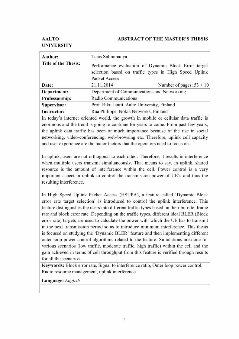
Date: 21.11.2014 Number of pages: 53 + 10 Department: Department of Communications and Networking Professorship: Radio Communications Supervisor: Prof. Riku Jantti, Aalto University, Finland Instructor: Rua Philippe, Nokia Networks, Finland In today’s internet oriented world, the growth in mobile or cellular data traffic is enormous and the trend is going to continue for years to come. From past few years, the uplink data traffic has been of much importance because of the rise in social networking, video-conferencing, web-browsing etc. Therefore, uplink cell capacity and user experience are the major factors that the operators need to focus on. In uplink, users are not orthogonal to each other. Therefore, it results in interference when multiple users transmit simultaneously. That means to say, in uplink, shared resource is the amount of interference within the cell. Power control is a very important aspect in uplink to control the transmission power of UE’s and thus the resulting interference. In High Speed Uplink Packet Access (HSUPA), a feature called ‘Dynamic Block error rate target selection’ is introduced to control the uplink interference. This feature distinguishes the users into different traffic types based on their bit rate, frame rate and block error rate. Depending on the traffic types, different ideal BLER (Block error rate) targets are used to calculate the power with which the UE has to transmit in the next transmission period so as to introduce minimum interference. This thesis is focused on studying the ‘Dynamic BLER’ feature and then implementing different outer loop power control algorithms related to the feature. Simulations are done for various scenarios (low traffic, moderate traffic, high traffic) within the cell and the gain achieved in terms of cell throughput from this feature is verified through results for all the scenarios. Keywords: Block error rate, Signal to interference ratio, Outer loop power control, Radio resource management, uplink interference.

Language: English

i

Acknowledgements

I received great support from several people throughout my thesis work directly or indirectly.

Firstly, I would like to express my sincere gratitude to Prof. Riku Jantti for guiding me throughput the thesis providing insightful inputs. Secondly, I would like to thank my instructor Rua Philippe, my Manager Pekka Marjelund and my technical advisor Pekka Kohonen for providing me an opportunity to carry out my thesis work at Nokia Networks. Rua Philippe and Pekka Kohonen have spent lot of time with me by providing valuable suggestions throughput my thesis work. I would also like to thank other team members Perttu Mella, Vesa Saako, Sheyam Domeja and Anna Sillanpaa for their valuable inputs and advices.

Finally, I would like to thank my parents and my friends for always being there with me providing all the support.

ii

Contents

List of Figures

List of Tables

List of Abbreviations

1 Introduction …………………………………………………………………………....1 1.1 Background …………………………………………………………………1 1.2 Scope of Thesis work …………………………………………………………….3 1.3 Outline of the Thesis ……………………………………………………………..3

2 High Speed Uplink Packet Access ………………………………………………….4

2.1 3GPP …………………………………………………………………………..….4 2.2 UMTS architecture ………………………………………………………………5 2.3 Standardization of HSUPA ……………………………………………………..5 2.4 R99 and HSUPA architecture for UTRAN…………………………………….6 2.5 Protocol layer architectural changes in HSUPA………………………………8

2.5.1 R99 radio protocol architecture …………………………………………..8 2.5.2 HSUPA protocol architectural changes ………………………………...10

2.6 HSUPA principles ……………………………………………………………...11 2.6.1 Fast layer 1 HARQ ……………………………………………………….11 2.6.2 HSUPA Node B scheduling ……………………………………………..12 2.6.3 Two TTI lengths in HSUPA ……………………………………………..13 2.6.4 HSUPA channels ………………………………………………………….13

2.6.4.1 E-DCH dedicated physical data channel …………………………13 2.6.4.2 E-DCH dedicated physical control channel ……………………...14 2.6.4.3 E-DCH HARQ indicator channel …………………………………14 2.6.4.4 E-DCH relative grant channel …………………………………….14 2.6.4.5 E-DCH absolute grant channel ……………………………………14

2.7 Radio Resource management algorithms ……………………………………14 2.7.1 Resource management ……………………………………………………15 2.7.2 Admission control ………………………………………………………...16 2.7.3 Load control and congestion control ……………………………………16 2.7.4 Handover control ………………………………………………………….17 2.7.5 Transport format selection by UE ……………………………………….18 2.7.6 Power control ……………………………………………………………...18

iii

2.7.6.1 Open loop power control …………………………………………….19 2.7.6.2 Closed loop power control …………………………………………..19

2.7.6.2.1 Inner closed loop power control …………………………...20 2.7.6.2.2 Outer closed loop power control …………………………...20

3 ‘Dynamic HSUPA BLER’ overview ………………………………………………21

3.1 Description ……………………………………………………………………...21 3.2 Functional split of OLPC module …………………………………………….23

3.2.1 OLPC entity ……………………………………………………………….23 3.2.2 OLPC controller …………………………………………………………..26

3.3 Shortcomings of the feature …………………………………………………...26 3.3.1 High HSUPA traffic in the cell ………………………………………….26 3.3.2 Low HSUPA traffic in the cell …………………………………………..27

4 Simulator implementation ………………………………………………………….28

4.1 Total uplink load factor of a cell ……………………………………………...29 4.2 Dynamic BLER, ΔSIR and target SIR ……………………………………….29 4.3 Uplink load factor per user …………………………………………………….29

4.3.1 DPCCH load factor ……………………………………………………….30 4.3.2 HS-DPCCH load factor …………………………………………………..30 4.3.3 E-DPCCH load factor …………………………………………………….32 4.3.4 E-DPDCH load factor ……………………………………………………32 4.3.5 Load factor per user ………………………………………………………35

4.4 Activity factor of users ………………………………………………………..35 4.5 Average user throughput and cell throughput ………………………………35

5 Analysis and simulation results ……………………………………………………37

5.1 With 10 HSUPA users in the cell ……………………………………………..37 5.1.1 Total uplink load factor …………………………………………………..37 5.1.2 Dynamic BLER, ΔSIR and target SIR ………………………………….37 5.1.3 Load factor of uplink channels …………………………………………..38 5.1.4 Average user throughput and cell throughput …………………………39

5.2 With 1 HSUPA user in the cell ………………………………………………41 5.3 With 72 HSUPA users in the cell ……………………………………………44

6 Conclusion …………………………………………………………………………….46

iv

References …………………………………………………………………………………48

Annexure 1 ………………………………………………………………………………...50

Annexure 2 ………………………………………………………………………………...52

v

List of Figures

2.1 UMTS system level architecture ………………………………………………….5

2.2 UTRAN architecture ……………………………………………………………….7

2.3 Radio interface protocol architecture ……………………………………………10

2.4 HSUPA user plane protocol architecture ……………………………………….11

2.5 ARQ and HARQ in HSUPA ……………………………………………………..12

2.6 RRM functionalities in HSUPA …………………………………………………15

2.7 Resource allocation control with HSUPA ……………………………………...16

2.8 Load control thresholds …………………………………………………………..17

2.9 Outer loop power control ………………………………………………………...20

3.1 Functional split of OLPC ………………………………………………………...23

3.2 BLER window implementation …………………………………………………24

4.1 MAC-e PDU structure ……………………………………………………………34

4.2 MAC-I PDU structure ……………………………………………………………34

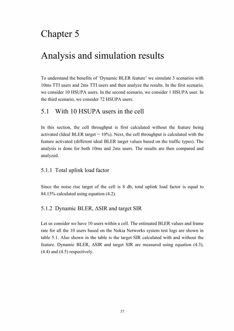
5.1 Cell throughput with 10 10ms users (HSUPA Dynamic BLER Feature inactive) ……………………………………………………………………………40

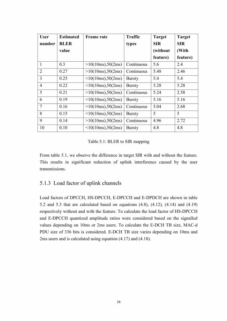
5.2 Cell throughput with 10 10ms users (HSUPA Dynamic BLER Feature active) ……………………………………………………………………………………………….40

5.3 Cell throughput with 10 2ms users (HSUPA Dynamic BLER Feature inactive) ……………………………………………………………………………………………….41

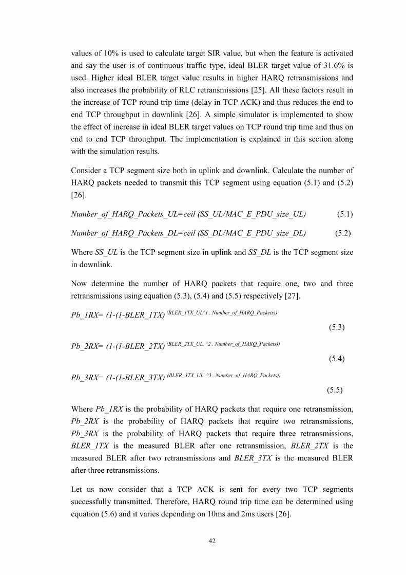
5.4 Cell throughput with 10 2ms users (HSUPA Dynamic BLER Feature active) ……………………………………………………………………………………………….41

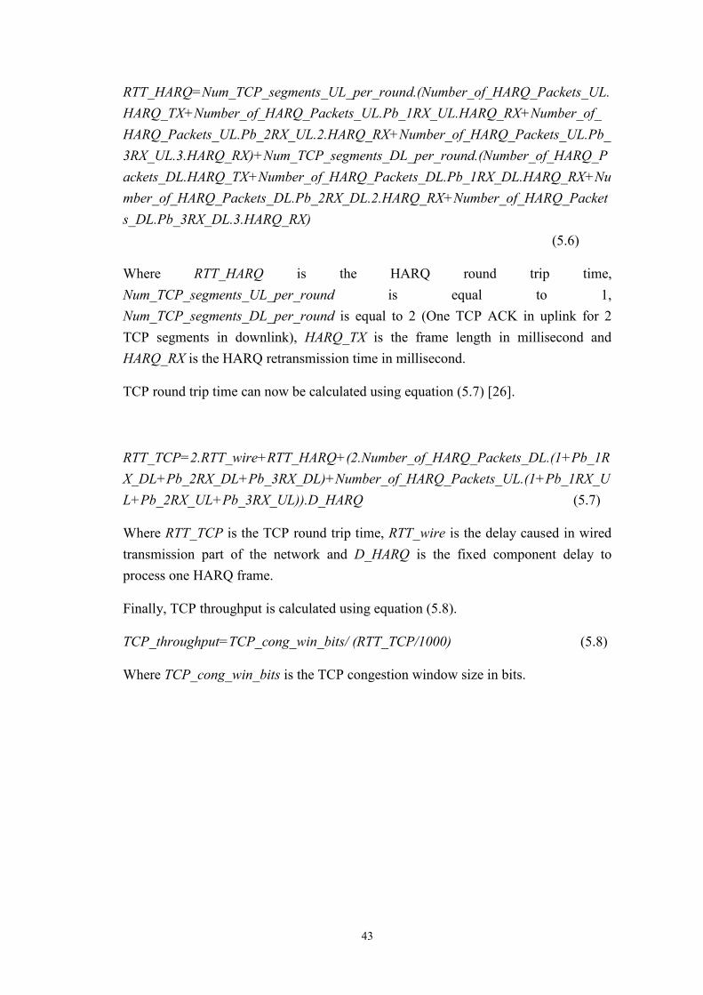
5.5 Relationship between uplink BLER, TCP round trip time and downlink TCP throughput with 1 HSUPA user in cell …………………………………………44

5.6 Cell throughput with 72 10ms users (Without correction to the feature) …...45

5.7 Cell throughput with 72 10ms users (With correction to the feature) ……….45

vi

List of Tables

2.1 3GPP release timeline ……………………………………………………………4

2.2 Comparison of R99, HSDPA and HSUPA …………………………………….6

2.3 RRM functionalities in UTRAN for R99 …………………………………….....7

2.4 RRM functionalities in UTRAN for HSUPA ………………………………….8

4.1 DPCCH power offsets …………………………………………………………...30

4.2 Quantization of the power offset for HS-DPCCH ……………………………31

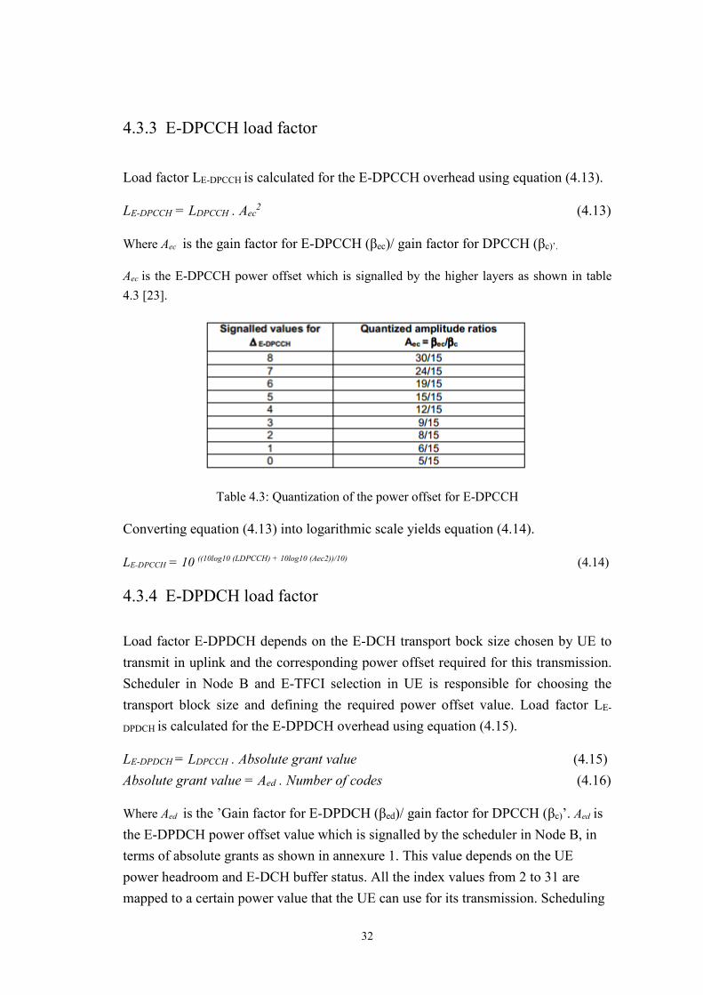
4.3 Quantization of the power offset for E-DPCCH ……………………………...32

5.1 BLER to SIR mapping …………………………………………………………..38

5.2 Load factors of channels (without feature) ……………………………………39

5.3 Load factors of channels (with feature) ………………………………………..39

vii

List of Abbreviations

1G First Generation

2G Second Generation

3G Third Generation

3GPP 3rd Generation Partnership Project

4G Fourth Generation

ARQ Automatic Repeat Request

BLER Block Error Rate

BMC Broadcast/Multicast

CN Core Network

CQI Channel Quality Indicator

CRC Cyclic Redundancy Checksum

CS Circuit Switched

DPCCH Dedicated Physical Control Channel

E-AGCH Enhanced Absolute Grant Channel

E-DCH Enhanced Dedicated Channel

E-DPCCH Enhanced Dedicated Physical Control Channel

E-DPDCH Enhanced Dedicated Physical Data Channel

E-HICH Enhanced HARQ Indicator Channel

E-RGCH Enhanced Relative Grant Channel

E-TFC E-DCH Transport Format Combination

EDGE Enhanced Data rates for GSM Evolution

FEC Forward Error Correction

viii

FP Frame Protocol

GPRS General Packet Radio Service

GSM Global System for Mobile communications

HARQ Hybrid Automatic Repeat Request

HS-DPCCH High Speed Dedicated Physical Control Channel

HSDPA High Speed Downlink Packet Access

HSUPA High Speed Uplink Packet Access

ILPC Inner Loop Power Control

IP Internet Protocol

MAC Medium Access Control

MEHO Mobile Evaluated Handover

MIMO Multiple Input Multiple Output

NEHO Network Evaluated handover

NRT Non Real Time

OLPC Outer Loop Power Control

P-CPICH Primary Common Pilot Channel

PDCP Packet Data Convergence Protocol

PRACH Primary Random Access Channel

PS Packet Switched

RAB Radio Access bearer

RLC Radio Link Control

RNC Radio network Controller

RRC Radio Resource Control

RRM Radio Resource Management

RSCP Received Signal Code Power

ix

RTWP Received Total Wideband Power

SDU Service Data Unit

SF Spreading Factor

SIR Signal to Interference Ratio

SRB Signalling Radio Bearer

TCP Transmission Control Protocol

TTI Transmission Time Interval

UE User Equipment

UMTS Universal Mobile Telecommunications Systems

UTRAN UMTS Terrestrial Radio Access Network

x

Chapter 1

Introduction

The first chapter gives a background on the thesis work and also defines the problem statement for the thesis. This chapter also gives a clear perspective to the reader about the scope of the thesis. The last section of this chapter gives an outline on the structure of the thesis.

1.1 Background Mobile communication systems have undergone significant changes over the past few decades. Cellular networks have evolved from the basic 1G (First Generation) analogue network or voice-only network, to 2G (Second generation) digital networks with text, multimedia messaging and data transfers with low speeds focusing on capacity and coverage, to 3G (Third Generation) or UMTS (Universal Mobile Telecommunications System) networks with data delivery rates of 384Kbps to 2Mbps focusing on true mobile broadband experience. The deployment of 4G (Fourth Generation) networks or the all IP (Internet Protocol) networks has widely increased in recent times and data rates of 100Mbps to 1Gbps are being achieved which provides access to wide range of mobile applications and services. The advancement in the wireless access technologies are to cater to the customer needs [1].

Mobile network traffic is increasing rapidly year after year and by 2017 more than 90% of the world is said to have 2G connections, 85% of the world is said to have 3G connections and 50% is said to have 4G connections [2]. The reason for this tremendous growth is the availability of innovative mobile applications like video conferencing, gaming, internet banking, mobile TV, streaming, social networking, health monitoring etc which has revolutionized the way people communicate [3].

The cellular networks should keep up with the growing demand for mobile traffic. 4G networks are undoubtedly far better than 3G in terms of speed, usability etc. But, since 4G networks are still not widely deployed all over the world and also since 4G networks tend to have shorter coverage range in some parts of the world, it is

1

necessary to maintain and optimize the 3G networks for at least few more years. To cater to all the above mentioned requirements, an enhanced version of 3G communication networks is introduced to have higher data speeds and capacity. In downlink, the enhanced 3G version is called high speed downlink packet access, reaching data rates of around 100 Mbps with the use of multiple carrier and MIMO (Multiple Input Multiple Output) technologies [4]. In uplink, the enhanced version is called high speed uplink packet access, reaching data rates of around 35 Mbps with the use of MIMO and higher modulation technologies [5].

In HSDPA (High Speed Downlink Packet Access), such high data rates are possible due to the new functionalities such as fast scheduling, fast retransmissions, adaptive modulation and coding, extended multi-code transmissions etc. In downlink, since channelization codes are the limiting factor for capacity, all these new functionalities make efficient use of channelization codes and thus increases downlink capacity [6]. In HSUPA (High Speed Uplink Packet Access), such high data rates are possible due to fast scheduling, fast retransmissions, multi-code transmissions, shorter transmission time interval etc. In uplink, since interference is the limiting factor for capacity, these new functionalities reduce the overall interference of the system and thus increase the uplink capacity [7].

In HSUPA, since interference is the capacity limiting factor, efficient power control mechanisms can reduce the interference resulted from each user in uplink. The power control procedure involves measuring the quality of the channel or transport block error rate in fixed time intervals. Based on the measurements, an algorithm is used to define the base station output power for each user, to achieve sufficient uplink quality of service in the subsequent transmissions. The base station output power for each user is calculated depending on the target SIR (Signal to Interference Ratio) required as defined by outer loop power control. Target SIR is calculated based on the measured BLER (Block Error Ratio) and ideal BLER target set during radio network planning [8]. Nokia Networks has introduced a new feature called ‘Dynamic HSUPA BLER’ which has an efficient power control algorithm to define and to modify the base station output power granted for each HSUPA user dynamically, depending on the channel quality and the type of uplink data transmission. It classifies the user into different traffic types based on the frame rate and FP (Frame Protocol) bit rate, and then uses different ideal BLER target values for each traffic type to determine the target SIR required for achieving sufficient uplink quality. The overall gain achieved from this new feature is the improvement in cell throughput due to the reduction of uplink interference within the cell [9]. The feature is better understood in the following chapters.

2

1.2 Scope of Thesis work The thesis work is focused on evaluating the performance improvement provided by ‘Dynamic HSUPA BLER’ feature. Firstly, we discuss about the feature from implementation point of view. Then, we compare the results of with and without the feature by implementing a simulator to calculate the cell throughput and average user throughput. Then, we discuss the two shortcomings of the feature under very low traffic and very high traffic in the cell. Then, we discuss the solutions to those problems with the help of another simple simulation. We then determine the gain in cell throughput before and after the solution for those problems.

We also discuss on some of the questions mentioned below in the coming chapters: Why ‘Dynamic HSUPA BLER’ feature? What is the gain achieved in terms of cell throughput? What are the other factors to be considered to gain maximum outcome from the feature? How are those factors taken care off?

1.3 Outline of the Thesis The structure of the thesis is mentioned below: Chapter 2 gives an introduction to high speed uplink packet access system architecture and protocol architecture. It also explains all the new principles introduced in HSUPA along with the description of new channels introduced. Also explained are the radio resource management algorithms like power control, handover control, load control, admission control, packet scheduler etc. This chapter forms a basis for understanding the entire thesis. Chapter 3 describes the ‘Dynamic HSUPA BLER’ feature from the implementation point of view. The major modifications are involved in outer loop power control algorithms and are discussed thoroughly. Chapter 4 describes the methodology of implementing the simulator needed to evaluate ‘Dynamic HSUPA BLER’ feature. Chapter 5 describes the simulation results and also discusses on the solutions for the already mentioned shortcomings of the feature. Chapter 6 gives the conclusion for the thesis work.

3

Chapter 2

High Speed Uplink Packet Access

The aim of this chapter is to introduce the functionality changes in HSUPA with respect to Release 99, explain the protocol architecture of R99 and HSUPA and also to explain various principles involved in HSUPA. This chapter also gives a general overview on radio resource management functionalities.

2.1 3GPP The term 3GPP stands for ’Third Generation Partnership Project’. 3GPP is a telecommunication forum and their sole purpose is to create technical specifications and technical reports for a 3rd generation mobile system based on the evolved GSM (Global System for Mobile Communication Networks) core networks and the radio access technologies supported. 3GPP also has the responsibility of approving and maintaining the specifications and reports which are to be used globally.

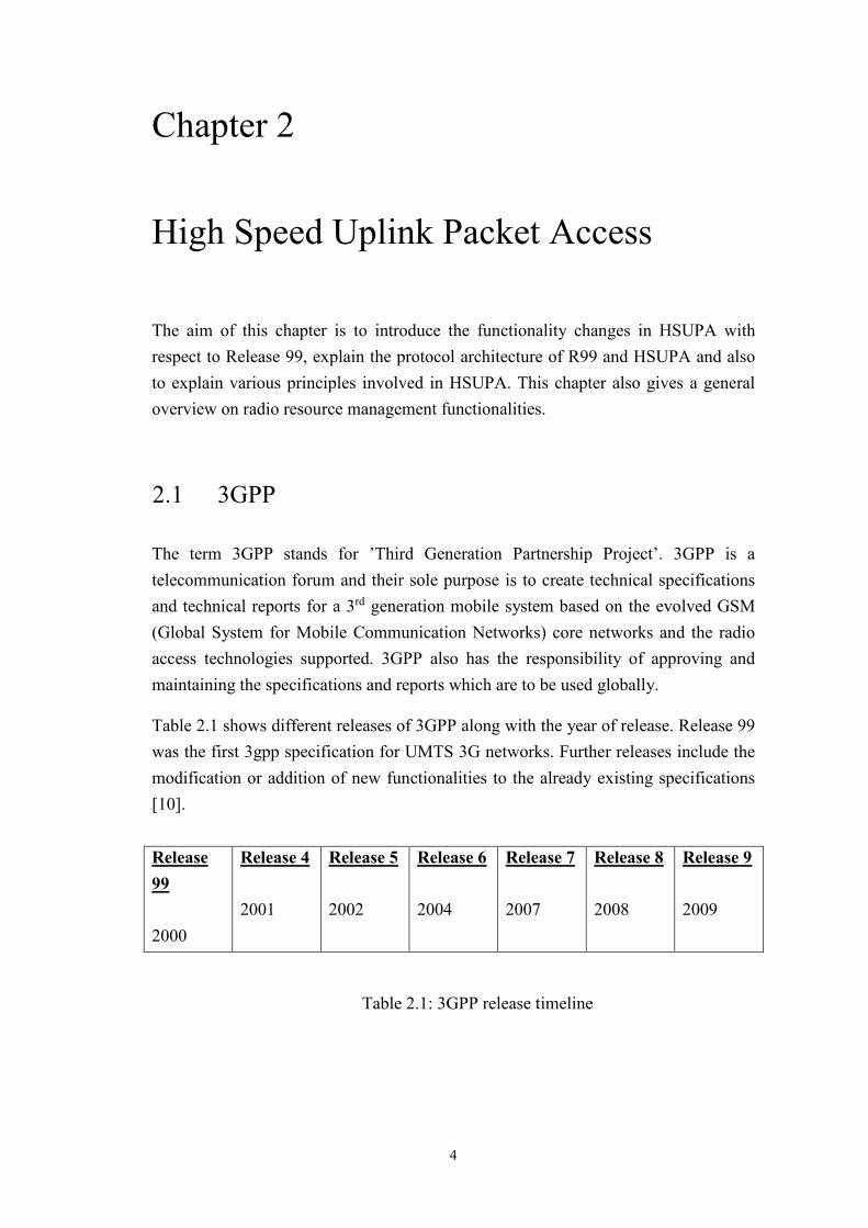
Table 2.1 shows different releases of 3GPP along with the year of release. Release 99 was the first 3gpp specification for UMTS 3G networks. Further releases include the modification or addition of new functionalities to the already existing specifications [10]. Release 99 2000

Release 4 2001

Release 5 2002

Release 6 2004

Release 7 2007

Release 8 2008

Release 9 2009

Table 2.1: 3GPP release timeline

4

2.2 UMTS architecture

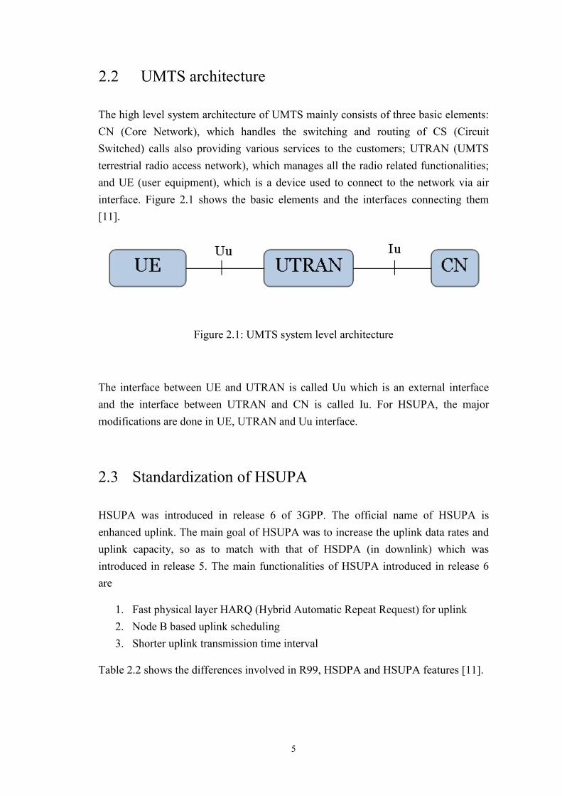
The high level system architecture of UMTS mainly consists of three basic elements: CN (Core Network), which handles the switching and routing of CS (Circuit Switched) calls also providing various services to the customers; UTRAN (UMTS terrestrial radio access network), which manages all the radio related functionalities; and UE (user equipment), which is a device used to connect to the network via air interface. Figure 2.1 shows the basic elements and the interfaces connecting them [11].

Figure 2.1: UMTS system level architecture

The interface between UE and UTRAN is called Uu which is an external interface and the interface between UTRAN and CN is called Iu. For HSUPA, the major modifications are done in UE, UTRAN and Uu interface.

2.3 Standardization of HSUPA HSUPA was introduced in release 6 of 3GPP. The official name of HSUPA is enhanced uplink. The main goal of HSUPA was to increase the uplink data rates and uplink capacity, so as to match with that of HSDPA (in downlink) which was introduced in release 5. The main functionalities of HSUPA introduced in release 6 are

1. Fast physical layer HARQ (Hybrid Automatic Repeat Request) for uplink 2. Node B based uplink scheduling 3. Shorter uplink transmission time interval

Table 2.2 shows the differences involved in R99, HSDPA and HSUPA features [11].

5

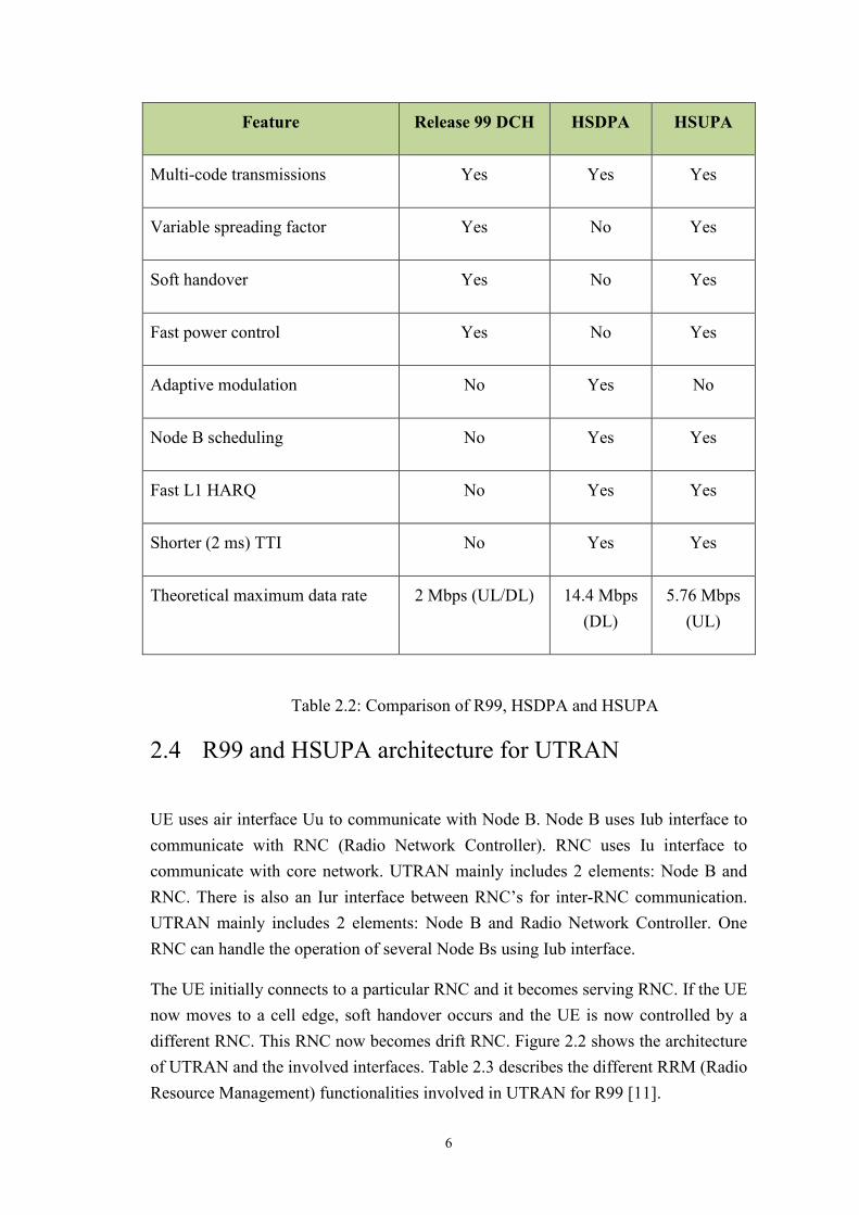
Feature Release 99 DCH HSDPA HSUPA

Multi-code transmissions Yes Yes Yes

Variable spreading factor Yes No Yes

Soft handover Yes No Yes

Fast power control Yes No Yes

Adaptive modulation No Yes No

Node B scheduling No Yes Yes

Fast L1 HARQ No Yes Yes

Shorter (2 ms) TTI No Yes Yes

Theoretical maximum data rate 2 Mbps (UL/DL) 14.4 Mbps (DL)

5.76 Mbps (UL)

Table 2.2: Comparison of R99, HSDPA and HSUPA

2.4 R99 and HSUPA architecture for UTRAN UE uses air interface Uu to communicate with Node B. Node B uses Iub interface to communicate with RNC (Radio Network Controller). RNC uses Iu interface to communicate with core network. UTRAN mainly includes 2 elements: Node B and RNC. There is also an Iur interface between RNC’s for inter-RNC communication. UTRAN mainly includes 2 elements: Node B and Radio Network Controller. One RNC can handle the operation of several Node Bs using Iub interface.

The UE initially connects to a particular RNC and it becomes serving RNC. If the UE now moves to a cell edge, soft handover occurs and the UE is now controlled by a different RNC. This RNC now becomes drift RNC. Figure 2.2 shows the architecture of UTRAN and the involved interfaces. Table 2.3 describes the different RRM (Radio Resource Management) functionalities involved in UTRAN for R99 [11].

6

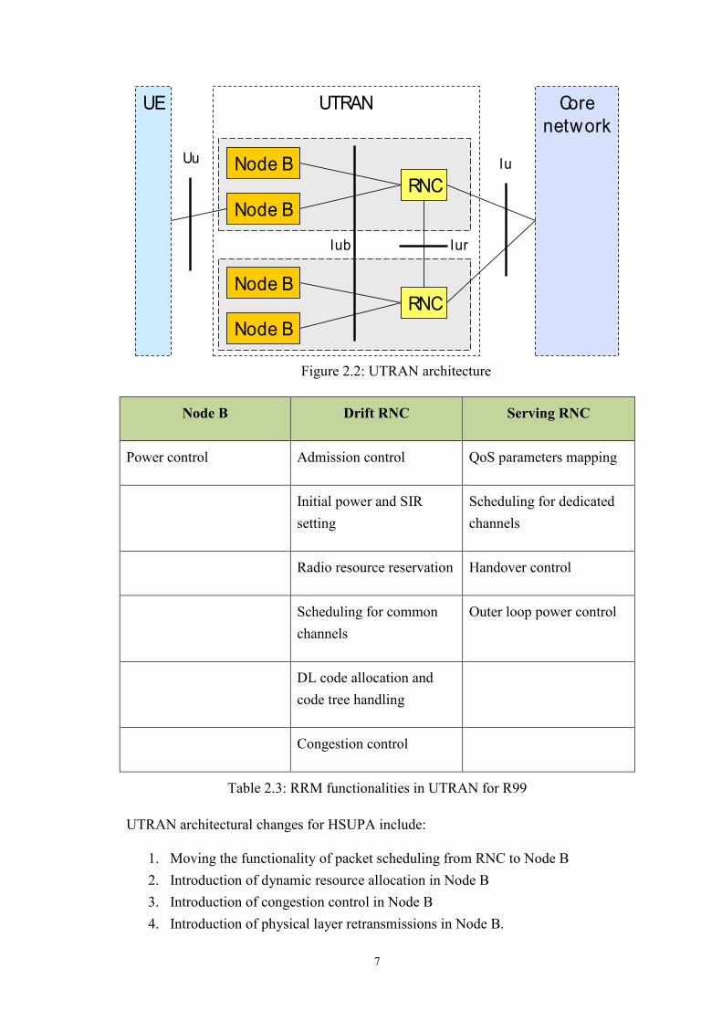
Figure 2.2: UTRAN architecture

Node B Drift RNC Serving RNC

Power control Admission control QoS parameters mapping

Initial power and SIR setting

Scheduling for dedicated channels

Radio resource reservation Handover control

Scheduling for common channels

Outer loop power control

DL code allocation and code tree handling

Congestion control

Table 2.3: RRM functionalities in UTRAN for R99

UTRAN architectural changes for HSUPA include:

1. Moving the functionality of packet scheduling from RNC to Node B 2. Introduction of dynamic resource allocation in Node B 3. Introduction of congestion control in Node B 4. Introduction of physical layer retransmissions in Node B.

UTRAN

RNC

RNC

UE Core network

IuUu Node B

Node B

IurIub

Node B

Node B

7

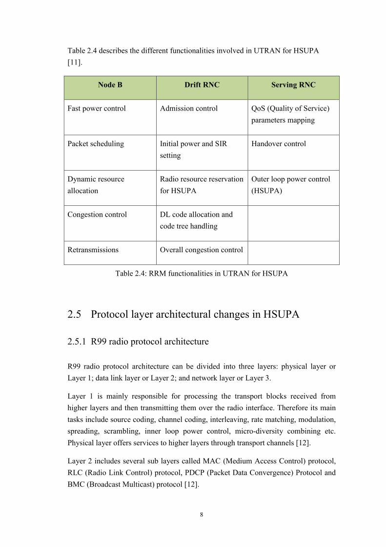
Table 2.4 describes the different functionalities involved in UTRAN for HSUPA [11].

Node B Drift RNC Serving RNC

Fast power control Admission control QoS (Quality of Service) parameters mapping

Packet scheduling Initial power and SIR setting

Handover control

Dynamic resource allocation

Radio resource reservation for HSUPA

Outer loop power control (HSUPA)

Congestion control DL code allocation and code tree handling

Retransmissions Overall congestion control

Table 2.4: RRM functionalities in UTRAN for HSUPA

2.5 Protocol layer architectural changes in HSUPA

2.5.1 R99 radio protocol architecture R99 radio protocol architecture can be divided into three layers: physical layer or Layer 1; data link layer or Layer 2; and network layer or Layer 3.

Layer 1 is mainly responsible for processing the transport blocks received from higher layers and then transmitting them over the radio interface. Therefore its main tasks include source coding, channel coding, interleaving, rate matching, modulation, spreading, scrambling, inner loop power control, micro-diversity combining etc. Physical layer offers services to higher layers through transport channels [12].

Layer 2 includes several sub layers called MAC (Medium Access Control) protocol, RLC (Radio Link Control) protocol, PDCP (Packet Data Convergence) Protocol and BMC (Broadcast Multicast) protocol [12].

8

The main tasks of MAC include multiplexing of several UE’s to the shared radio resource, mapping and multiplexing of logical channels within one UE to transport channels, prioritizing between services of same UE, prioritizing between different UE’s, traffic volume measurements, channel type switching, ciphering and selecting suitable transport format for each transport channel. MAC offers transport layer services to its higher layers through logical channels.

The main tasks of RLC include segmentation and reassembly of control and user data, concatenation, padding, duplicate avoidance and removal, sequence number checking, SDU (Service Data Unit) discard, error correction or retransmission, flow control and ciphering. RLC offers services to its higher layers. RLC can provide three kinds of services to a logical channel:

1. Transparent mode, where header is not added to data in RLC. 2. Unacknowledged mode, where flow control RLC retransmissions are not

possible. 3. Acknowledged mode, where flow control and RLC retransmissions are

enabled.

PDCP is used mainly for compressing the user data such as IP header compression and in sequence delivery of packet data, whereas BMC is used mainly for cell broadcasting and multicast broadcasting services.

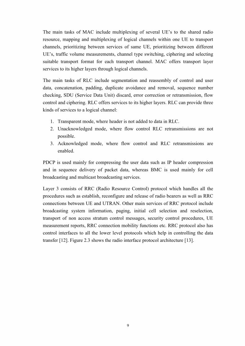
Layer 3 consists of RRC (Radio Resource Control) protocol which handles all the procedures such as establish, reconfigure and release of radio bearers as well as RRC connections between UE and UTRAN. Other main services of RRC protocol include broadcasting system information, paging, initial cell selection and reselection, transport of non access stratum control messages, security control procedures, UE measurement reports, RRC connection mobility functions etc. RRC protocol also has control interfaces to all the lower level protocols which help in controlling the data transfer [12]. Figure 2.3 shows the radio interface protocol architecture [13].

9

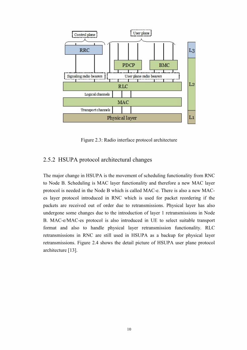
Figure 2.3: Radio interface protocol architecture

2.5.2 HSUPA protocol architectural changes The major change in HSUPA is the movement of scheduling functionality from RNC to Node B. Scheduling is MAC layer functionality and therefore a new MAC layer protocol is needed in the Node B which is called MAC-e. There is also a new MAC-es layer protocol introduced in RNC which is used for packet reordering if the packets are received out of order due to retransmissions. Physical layer has also undergone some changes due to the introduction of layer 1 retransmissions in Node B. MAC-e/MAC-es protocol is also introduced in UE to select suitable transport format and also to handle physical layer retransmission functionality. RLC retransmissions in RNC are still used in HSUPA as a backup for physical layer retransmissions. Figure 2.4 shows the detail picture of HSUPA user plane protocol architecture [13].

10

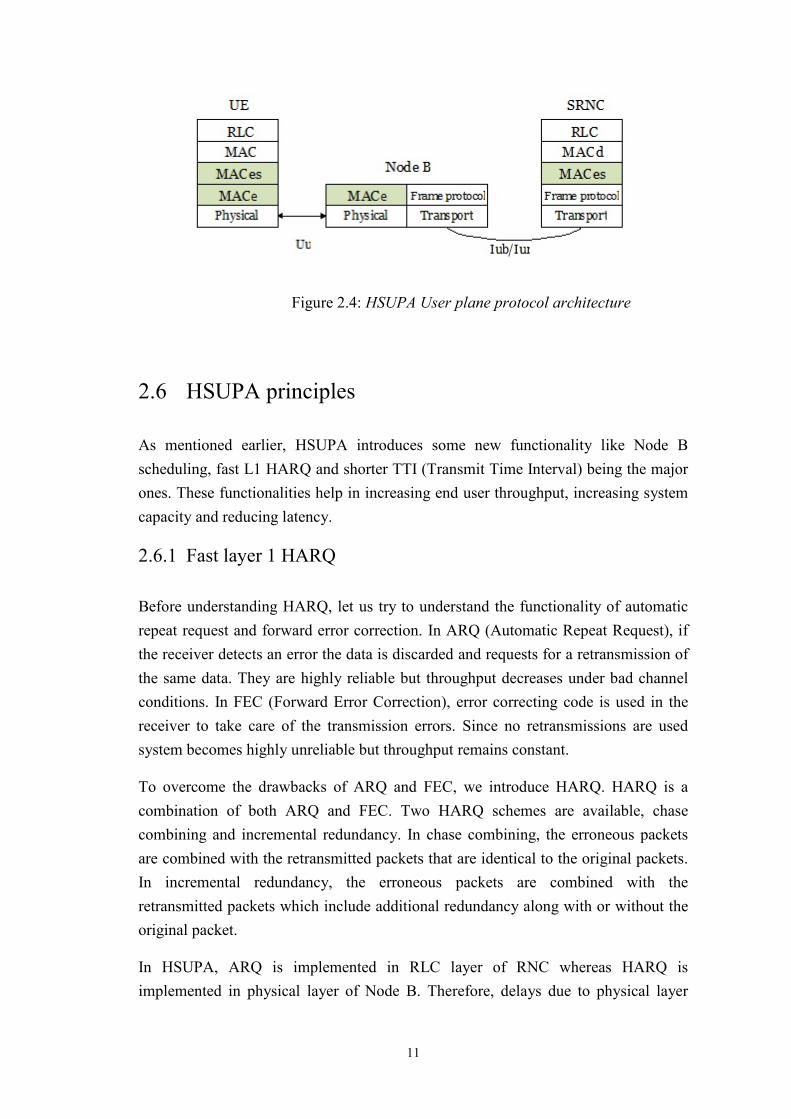
Figure 2.4: HSUPA User plane protocol architecture

2.6 HSUPA principles As mentioned earlier, HSUPA introduces some new functionality like Node B scheduling, fast L1 HARQ and shorter TTI (Transmit Time Interval) being the major ones. These functionalities help in increasing end user throughput, increasing system capacity and reducing latency.

2.6.1 Fast layer 1 HARQ Before understanding HARQ, let us try to understand the functionality of automatic repeat request and forward error correction. In ARQ (Automatic Repeat Request), if the receiver detects an error the data is discarded and requests for a retransmission of the same data. They are highly reliable but throughput decreases under bad channel conditions. In FEC (Forward Error Correction), error correcting code is used in the receiver to take care of the transmission errors. Since no retransmissions are used system becomes highly unreliable but throughput remains constant.

To overcome the drawbacks of ARQ and FEC, we introduce HARQ. HARQ is a combination of both ARQ and FEC. Two HARQ schemes are available, chase combining and incremental redundancy. In chase combining, the erroneous packets are combined with the retransmitted packets that are identical to the original packets. In incremental redundancy, the erroneous packets are combined with the retransmitted packets which include additional redundancy along with or without the original packet.

In HSUPA, ARQ is implemented in RLC layer of RNC whereas HARQ is implemented in physical layer of Node B. Therefore, delays due to physical layer

11

retransmissions are much less compared to RLC retransmissions. Thus, physical channels can operate at higher error rate which can increase system capacity. Due to the physical layer retransmissions, RLC retransmissions are significantly low.

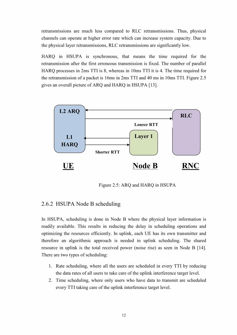
HARQ in HSUPA is synchronous, that means the time required for the retransmission after the first erroneous transmission is fixed. The number of parallel HARQ processes in 2ms TTI is 8, whereas in 10ms TTI it is 4. The time required for the retransmission of a packet is 16ms in 2ms TTI and 40 ms in 10ms TTI. Figure 2.5 gives an overall picture of ARQ and HARQ in HSUPA [13].

Figure 2.5: ARQ and HARQ in HSUPA

2.6.2 HSUPA Node B scheduling In HSUPA, scheduling is done in Node B where the physical layer information is readily available. This results in reducing the delay in scheduling operations and optimizing the resources efficiently. In uplink, each UE has its own transmitter and therefore an algorithmic approach is needed in uplink scheduling. The shared resource in uplink is the total received power (noise rise) as seen in Node B [14]. There are two types of scheduling:

1. Rate scheduling, where all the users are scheduled in every TTI by reducing the data rates of all users to take care of the uplink interference target level.

2. Time scheduling, where only users who have data to transmit are scheduled every TTI taking care of the uplink interference target level.

L2 ARQ

L1

HARQ Layer 1

RLC

UE Node B RNC

Shorter RTT

Longer RTT

12

In HSUPA, scheduling operation takes place in MAC layer. UE sends happy bit to Node B indicating if it can transmit at a higher data rate than currently allocated or not. Node B which has information about uplink noise rise and power levels, decides to increase or decrease the power granted to UE. The UE correspondingly adjusts its transmission power.

2.6.3 Two TTI lengths in HSUPA

HSUPA supports both 2 ms and 10 ms transmission time intervals. The shorter TTI of 2ms is used to reduce the delay caused by retransmissions compared to 10ms TTI. If the number of retransmissions increases significantly as in the case of cell edge user, downlink signalling power increases and hence Node B consumes a lot of transmission power. Therefore it is necessary to have 10 ms TTI for cell edge users in HSUPA where the downlink signalling can be reduced compared to 2 ms TTI [14].

2.6.4 HSUPA channels In HSUPA, UE has a new dedicated uplink transport channel E-DCH (Enhanced Dedicated Channel) in the uplink. It supports enhanced features as compared to that of DCH (Dedicated Channel). The two major differences between E-DCH and DCH are:

1. A UE can have only one E-DCH transport channel whereas it can have multiple DCH transport channels configured.

2. HARQ functionality is supported for E-DCH.

The E-DCH transport channel is now mapped to multiple E-DPDCH (Enhanced Downlink Physical Data Channel) uplink physical channels for physical layer transmission. Both DCH and E-DCH can co-exist in the same UE since both are working in parallel. The E-DPCCH (Enhanced Downlink Physical Control Channel) is sent in parallel to E-DPDCH which carries all the control information of E-DPDCH. There also exist three new downlink physical channels E-HICH (Enhanced HARQ Indicator Channel), E-RGCH (Enhanced Relative Grant Channel) and E-AGCH (Enhanced Absolute Grant Channel) for HARQ indication and scheduling purposes [14].

2.6.4.1 E-DCH dedicated physical data channel E-DPDCH is an uplink physical channel used for transmitting data received from E-

13

DCH transport channel. E-DPDCH exists in parallel with DPDCH, DPCCH and HS-DPCCH of R99. E-DPDCH supports physical layer HARQ, Node B scheduling, minimum spreading factor of 2, TTI lengths of 2ms and multi-code transmission. E-DPDCH is transmitted in parallel with DPCCH as it needs information on SIR, power control bits and channel estimation. 2.6.4.2 E-DCH dedicated physical control channel

E-DPCCH is an uplink physical channel used for carrying out-of-band information about E-DPDCH. E-DPCCH uses a spreading factor of 256 and carries information such as E-TFCI (Enhanced Transport Format Combination Indicator) which indicates the transport format combination, RSN (Retransmission Sequence Number) which indicates the HARQ sequence number of the transport block and happy bit which indicates if the UE can transmit with higher power or not.

2.6.4.3 E-DCH HARQ indicator channel

E-HICH is a downlink physical channel used to send ACK or NACK for every E-DPDCH data transmitted in uplink i.e. for every TTI.

2.6.4.4 E-DCH relative grant channel

E-RGCH is a downlink physical channel used to increase or decrease the uplink transmission power of E-DPDCH every TTI. The change in transmission power happens in small steps.

2.6.4.5 E-DCH absolute grant channel

E-AGCH is a downlink physical channel used to transmit the absolute maximum transmission power value based on the Node B scheduler. This is the maximum power with which the UE can transmit data in E-DPDCH.

2.7 Radio Resource management algorithms

Radio Resource Management is a mechanism in the cellular communication systems, which uses different algorithms to optimize the radio resource utilization by controlling the system level co-channel interference and other radio transmission characteristics, to serve the user with a better quality of service [11].

14

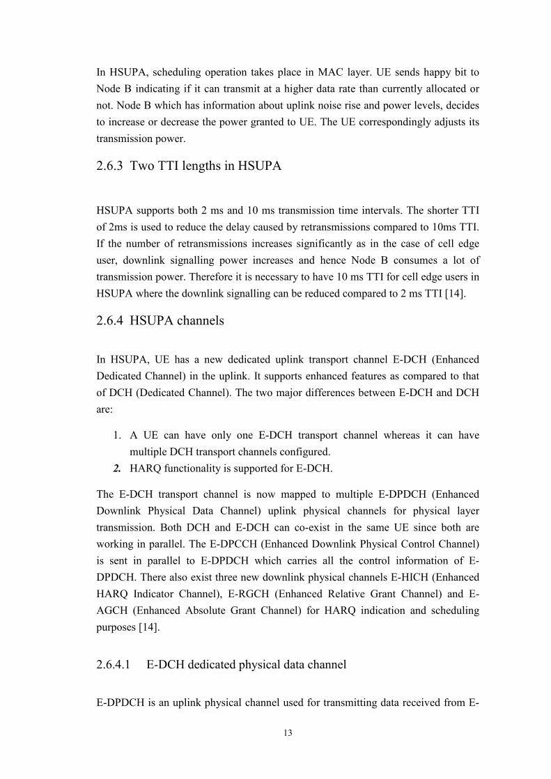
HSUPA RRM includes functionalities in RNC, Node B and UE. HSUPA RRM in RNC is responsible for allocating resources to both DCH and E-DCH users. HSUPA RRM in Node B is responsible for sharing the resources between different HSUPA UE’s. HSUPA RRM in UE is responsible to choose the transport block size based on the resources allocated to it by Node B and also based on the buffer size. Figure 2.6 describes all the RRM functionalities of HSUPA in general [11].

Figure 2.6: RRM functionalities in HSUPA

2.7.1 Resource management Noise rise is defined as the ratio of total received wideband power to the noise power. The received power consists of intra-cell interference from DCH and E-DCH connections, inter-cell interference and thermal noise. RNC defines the maximum uplink interference target or the noise rise for the Node B based on the radio network planning. The resources for DCH connections (scheduled and non-scheduled) are managed by RNC and the resources for E-DCH connections are managed by Node B. Resource allocation control with HSUPA is shown in figure 2.7 [11].

15

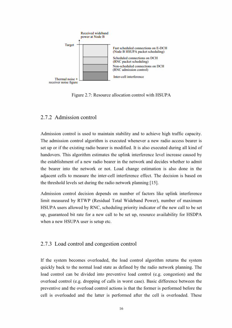
Figure 2.7: Resource allocation control with HSUPA

2.7.2 Admission control Admission control is used to maintain stability and to achieve high traffic capacity. The admission control algorithm is executed whenever a new radio access bearer is set up or if the existing radio bearer is modified. It is also executed during all kind of handovers. This algorithm estimates the uplink interference level increase caused by the establishment of a new radio bearer in the network and decides whether to admit the bearer into the network or not. Load change estimation is also done in the adjacent cells to measure the inter-cell interference effect. The decision is based on the threshold levels set during the radio network planning [15].

Admission control decision depends on number of factors like uplink interference limit measured by RTWP (Residual Total Wideband Power), number of maximum HSUPA users allowed by RNC, scheduling priority indicator of the new call to be set up, guaranteed bit rate for a new call to be set up, resource availability for HSDPA when a new HSUPA user is setup etc.

2.7.3 Load control and congestion control If the system becomes overloaded, the load control algorithm returns the system quickly back to the normal load state as defined by the radio network planning. The load control can be divided into preventive load control (e.g. congestion) and the overload control (e.g. dropping of calls in worst case). Basic difference between the preventive and the overload control actions is that the former is performed before the cell is overloaded and the latter is performed after the cell is overloaded. These

16

actions are performed by measuring both uplink and downlink interference periodically in the cell level.

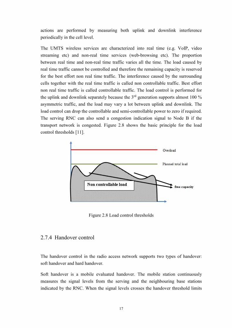
The UMTS wireless services are characterized into real time (e.g. VoIP, video streaming etc) and non-real time services (web-browsing etc). The proportion between real time and non-real time traffic varies all the time. The load caused by real time traffic cannot be controlled and therefore the remaining capacity is reserved for the best effort non real time traffic. The interference caused by the surrounding cells together with the real time traffic is called non controllable traffic. Best effort non real time traffic is called controllable traffic. The load control is performed for the uplink and downlink separately because the 3rd generation supports almost 100 % asymmetric traffic, and the load may vary a lot between uplink and downlink. The load control can drop the controllable and semi-controllable power to zero if required. The serving RNC can also send a congestion indication signal to Node B if the transport network is congested. Figure 2.8 shows the basic principle for the load control thresholds [11].

Figure 2.8 Load control thresholds

2.7.4 Handover control

The handover control in the radio access network supports two types of handover: soft handover and hard handover.

Soft handover is a mobile evaluated handover. The mobile station continuously measures the signal levels from the serving and the neighbouring base stations indicated by the RNC. When the signal levels crosses the handover threshold limits

17

set by RNC, the mobile station sends a measurement report to the RNC. Now, the RNC decides whether to add or remove cells from the mobile stations active set [11].

The following types of soft handovers are supported:

I. Handover between cells within one base station called softer handover. II. Handover between base stations within one RNC called intra-RNC soft

handover. III. Handover between base stations controlled by separate RNC’s called inter-

RNC soft handover.

Hard handover is classified into inter-frequency and intra-frequency hard handovers. Intra-frequency hard handover is a mobile evaluated handover while inter-frequency hard handover is a network-evaluated handover. Hard handover is lossless for non real time radio bearer but it causes a short disconnection for real time radio bearer.

2.7.5 Transport format selection by UE The transport format selection is done in MAC layer of UE. The UE receives information on the supported transport block sizes and the corresponding power offset values required to transmit the selected transport block. UE also has information on the priorities of the logical channels, E-DCH buffer status and also the maximum power with which it can transmit. Now, UE receives scheduling grants from Node B via E-AGCH or E-RGCH indicating the maximum power offset with which the UE can transmit every TTI. Depending on the scheduling grant, UE chooses the highest possible E-TFC value [14]. Node B packet scheduling and HARQ functionalities are already explained in section 2.6

2.7.6 Power control Power control is the most important and critical aspect of radio resource management, especially in uplink. In uplink, since all the users transmit at the same time within the same frequency, each one of them becomes interference to the rest and vice versa.

Consider there are two mobile stations UE1 and UE2 operating within the same frequency. Also consider that both are transmitting at same powers, but UE1 is nearer to the base station compared to UE2. Therefore, Node B receives more power from

18

UE1 than UE2 which results in masking of UE2 and thus blocking a large part of the cell. This situation is called near-far problem and has to be controlled by efficient power control mechanism [11].

There are two power control mechanisms in HSUPA called open loop power control and closed loop power control.

2.7.6.1 Open loop power control Open loop power control is performed in UE. In uplink open loop power control, UE measures the RSCP (Received Signal Code Power) of the active P-CPICH (Primary Common Pilot Channel) and some control parameters are transmitted by Node B on broadcast channel. The RSCP of CPICH is inversely proportional to the distance between UE and Node B. Based on this information, UE can estimate the path loss and thus the distance from the Node B. This helps in determining the required initial power for the first RACH (Random Access Channel) preamble to be transmitted, using equation (2.1) given below [16].

(2.1)

Where CPICHTXpwr is the downlink transmit power, ULint is the uplink interference and ULCI is the required carrier to interference ratio for uplink.

2.7.6.2 Closed loop power control

Closed loop power control operates both in uplink and downlink and it is a combination of inner and outer loop power control functionalities. The inner loop power control operates between User equipment and Node B. It controls the transmitted power of the UE to keep the received signal to interference ratio close to the target SIR. The target SIR is set by outer loop power control by measuring the quality of uplink data transmission. Quality is measured by calculating block error rate of the data frames sent by UE.

19

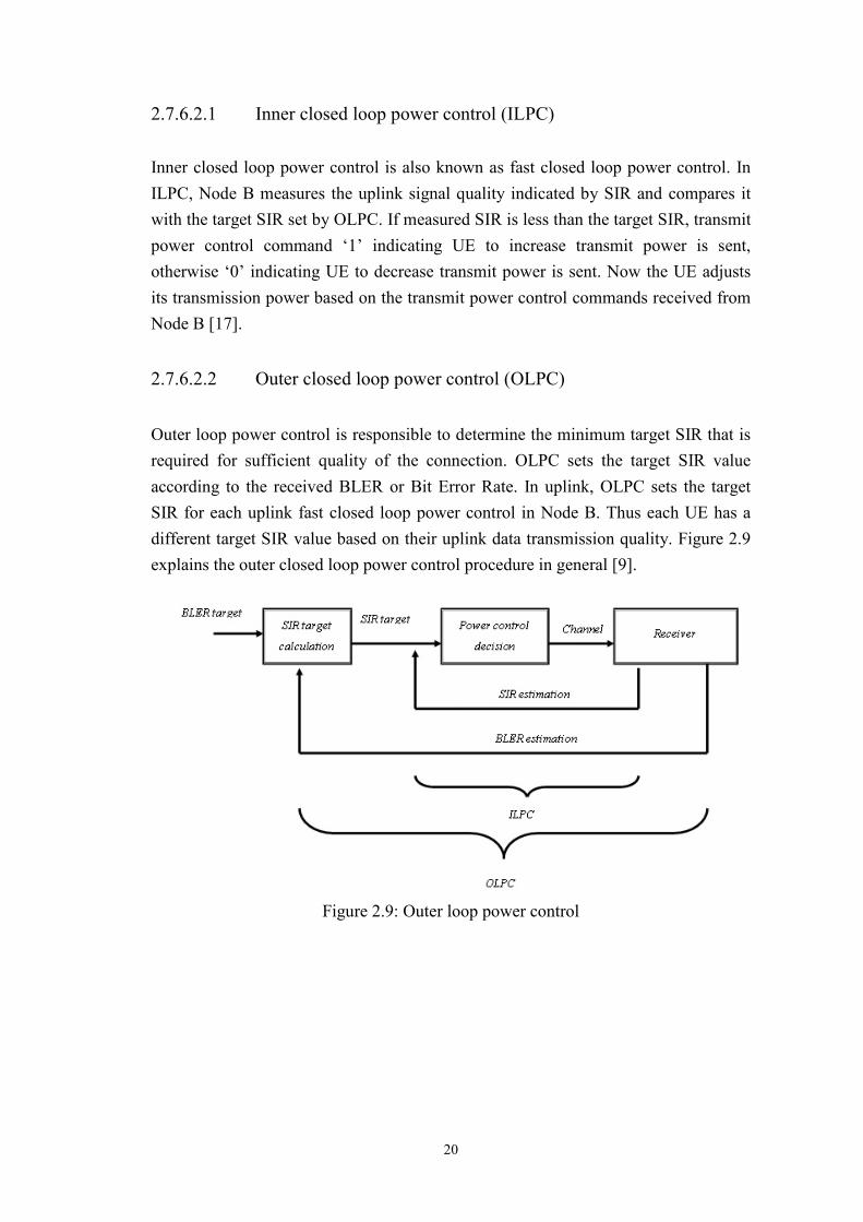
2.7.6.2.1 Inner closed loop power control (ILPC) Inner closed loop power control is also known as fast closed loop power control. In ILPC, Node B measures the uplink signal quality indicated by SIR and compares it with the target SIR set by OLPC. If measured SIR is less than the target SIR, transmit power control command ‘1’ indicating UE to increase transmit power is sent, otherwise ‘0’ indicating UE to decrease transmit power is sent. Now the UE adjusts its transmission power based on the transmit power control commands received from Node B [17]. 2.7.6.2.2 Outer closed loop power control (OLPC) Outer loop power control is responsible to determine the minimum target SIR that is required for sufficient quality of the connection. OLPC sets the target SIR value according to the received BLER or Bit Error Rate. In uplink, OLPC sets the target SIR for each uplink fast closed loop power control in Node B. Thus each UE has a different target SIR value based on their uplink data transmission quality. Figure 2.9 explains the outer closed loop power control procedure in general [9].

Figure 2.9: Outer loop power control

20

Chapter 3

‘Dynamic HSUPA BLER’ overview 3.1 Description In uplink, interference limits the capacity of a cell, and therefore it is necessary to share the uplink interference among HSUPA users within a cell in an optimized way. ‘Dynamic HSUPA BLER’ feature provides one such possibility by differentiating the HSUPA users into different traffic types based on several inputs such as frame rate, FP bit rate and number of HARQ retransmission information [18]. Outer loop power control of radio resource management module in RNC takes this responsibility of distinguishing the users. The frame rate information is obtained from the BLER window implementation in OLPC. It is explained clearly in later sections of this chapter. FP bit rate information is received from MAC-es module by calculating the data rate over complete frame window period. The number of HARQ retransmissions required to successfully transmit a transport block in uplink is obtained from HARQ module. The other job of OLPC is to measure the block error ratio of PS NRT bearers by checking the CRC (Cyclic Redundancy Check) values of each transport block received. Classification of traffic types is based on the following three criteria’s and the corresponding ideal BLER target values chosen are also mentioned below [9]:

1. If the percentage of UE packets in FP frame is greater than 90%, then we say that the PS NRT bearers can achieve peak data rates close to the bearer maximum. This type of user is classified into peak traffic type and ideal BLER target of 8% is used after zero HARQ retransmissions.

2. If the number of FP frames per second is less than or equal to 10 in case of

10ms TTI or less than or equal to 50 in case of 2ms TTI, then we say that the UE is transmitting data in bursts. This type of user is classified as bursty traffic type and ideal BLER target of 10% is used after 0 HARQ retransmissions.

21

3. If the number of FP frames per second are greater than 10 in case of 10ms TTI

or greater than 50 in case of 2ms TTI, then we say that the UE is transmitting data continuously. This type of user is classified as continuous traffic type and ideal BLER target of 10% is used after 1 HARQ retransmissions or we can say that ideal BLER target of √10 = 31.6% is used after 0 HARQ retransmissions.

Once the traffic type, ideal BLER target value and the measured BLER value for a particular user is available, the target SIR is calculated for PS NRT bearers in the OLPC module. Initial target SIR is fixed depending on signalling RAB (Radio Access bearer) quality of the user. The other task of this feature is to check for the possibility of traffic type transition in the users by measuring the frame rate, FP bit rate and BLER in short fixed time intervals. If there is a traffic type transition happening, then respective ideal BLER target values are chosen dynamically and the target SIR is recalculated based on the number and type of services associated with the UE. The rules for traffic type transitions and target SIR recalculations are mentioned below [9]:

1. If traffic state changes from peak to bursty or continuous and if SIR target is greater than initial SIR target, then use initial SIR target as new SIR target.

2. If traffic state changes from bursty or continuous to peak and if SIR target is less than initial SIR target, then use initial SIR target as new SIR target.

3. If traffic state changes from bursty to continuous or vice versa and if SIR target is greater than initial SIR target, then use initial SIR target as new SIR target.

The above mentioned SIR target recalculations are done depending on the number and type of services associated with the UE. Some conditions to be followed are mentioned below [9]:

1. If UE has only one PS (Packet Switched) entity and an SRB (Signalling Radio Bearer) entity, PS entity can request for SIR target adjustment irrespective of its activity states.

2. If UE has more PS entities and an SRB entity, then only PS active entity can request for SIR target adjustment.

3. If the UE has one or more PS entities, one CS (Circuit Switched) entity and an SRB entity, then only PS active entity can request for SIR target adjustment.

22

The detailed description for all the above mentioned procedures can be well understood in section 3.2.

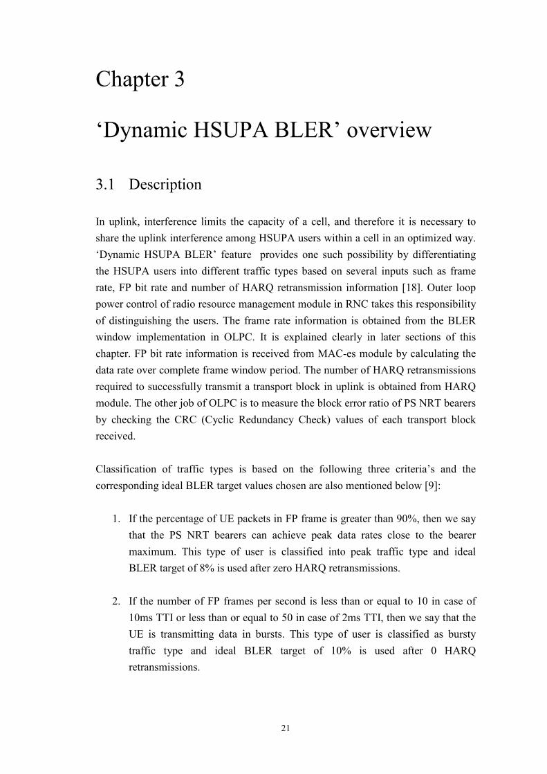
3.2 Functional split of OLPC module OLPC in RNC is divided into number of OLPC entities and one OLPC controller that control all the entities. In context of one call, there may be several services and each service has a traffic channel associated with it. Therefore, one call will have several OLPC entities (equal to the number of services in that call plus an additional signalling OLPC entity) and one OLPC controller. In HSUPA, since the traffic channel E-DCH can be spread across multiple (maximum 4) physical channels and carried over the air interface, there are 4 additional E-DCH OLPC entities. Figure 3.1 shows the functional split of uplink OLPC [16].

RNC

Node B -1 L1/ FP Node B-2

Figure 3.1: Functional split of OLPC

3.2.1 OLPC entity The major task of the OLPC entity is to monitor the uplink quality by measuring the block error rate of the data frames received and thereby calculating the needed SIR changes to have a sufficient quality for the service. The OLPC entities can be in one of the three states (active, semi-active or inactive) which are controlled by the OLPC

UL OLPC

UL OLPC entity 1

UL OLPC entity n

UL ILPC UL ILPC

23

controller. Active state entity can send either SIR target up or down command, semi-active entity can send only SIR target up command and inactive entity cannot send either SIR target up or down command. OLPC entity algorithms are classified based on whether E-DCH or DCH channels are used for the service.

Algorithm 1 is used when there is at least one E-DCH channel in the service [16]. Algorithm 1 is a three step process.

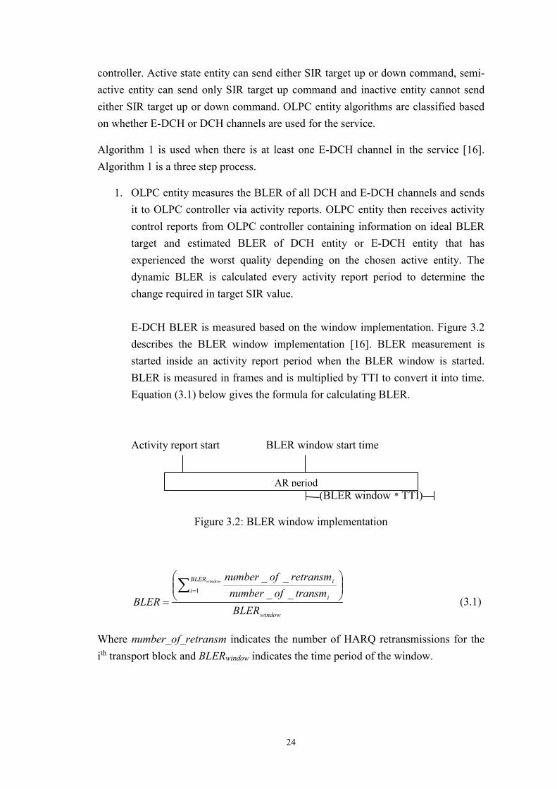
1. OLPC entity measures the BLER of all DCH and E-DCH channels and sends it to OLPC controller via activity reports. OLPC entity then receives activity control reports from OLPC controller containing information on ideal BLER target and estimated BLER of DCH entity or E-DCH entity that has experienced the worst quality depending on the chosen active entity. The dynamic BLER is calculated every activity report period to determine the change required in target SIR value. E-DCH BLER is measured based on the window implementation. Figure 3.2 describes the BLER window implementation [16]. BLER measurement is started inside an activity report period when the BLER window is started. BLER is measured in frames and is multiplied by TTI to convert it into time. Equation (3.1) below gives the formula for calculating BLER. Activity report start BLER window start time (BLER window * TTI)

Figure 3.2: BLER window implementation

window

BLER

ii

i

BLERtransmofnumber

retransmofnumber

BLER

window

=∑ =1 __

__

(3.1)

Where number_of_retransm indicates the number of HARQ retransmissions for the ith transport block and BLERwindow indicates the time period of the window.

AR period

24

DCH BLER is measured based on the last frame received before the activity report period ended given by equation (3.2).

TBs all of numberTBs ok not CRC of numberBLER = (3.2)

Dynamic BLER is then calculated from equation (3.3) or (3.4) depending on the situation.

BLER_EDCH)R_target(ideal_BLEveof_the_curDCH_slope_H_target_DCideal_BLERDCHER_target_dynamic_BL

−⋅++=

(3.3)

Where BLER_EDCH is the block error rate measured with E-DCH channel and DCH_slope_of_the_curve is a constant.

BLER_DCH)R_target(ideal_BLErve_of_the_cuEDCH_slopeCH_target_EDideal_BLEREDCHER_target_dynamic_BL

−⋅++=

(3.4)

Where BLER_DCH is the block error rate measured with DCH channel and EDCH_slope_of_the_curve is a constant.

Determine the SIR step change based on equation (3.5) if it is for DCH and equation (3.6) if it is for E-DCH.

BLERstepizeDCHt_DCHBLER_Targetep_sizesir_down_sHBLERstepsizeDCDCH)ER_Target_dynamic_BL(p_sizesir_up_ste

⋅=⋅−= 1

(3.5) Where stepsizeDCHBLER is a constant.

HBLERstepizeEDCEDCHTargetBLERsizestepdownsirCHBLERstepsizeEDEDCHTargetBLERdynamicsizestepupsir

⋅=⋅−=

_____)___1(___

(3.6) Where stepsizeEDCHBLER is a constant.

2. OLPC entity receives quality information from macro diversity and combining unit. The CRC’s of the frame transport blocks are checked. If all transport blocks are error free, SIR down step size is sent by the active entity. If any one of the transport block is erroneous, SIR up step size is sent by the active entity.

Algorithm 2 is used when there are only E-DCH channels in the call. OLPC entity receives either HARQ retransmission threshold information from MAC-es or HARQ failure information from frame protocol. If frame is ok, then BLER estimation is

25

equal to 0 else BLER estimation is equal to 1 [7]. Change in SIR (∆SIR) required is calculated using equation (3.7).

)_(_ tBLER_targeestimationBLERsizestepSIR −=∆ (3.7)

Where step_size is a constant and BLER_target is a fixed value obtained from OLPC controller.

3.2.2 OLPC controller The major task of OLPC controller is the selection of active entity and calculating the new SIR set point. All entities send activity reports to OLPC controller synchronously with fixed activity reporting period. Based on these activity reports, activity states of the entities are selected for the duration of next reporting period.

OLPC controller algorithm starts when an activity report is received from some OLPC entity. If the difference between the measured BLER and ideal BLER target for the entity that just sent activity report is greater than for the entity that has so far been selected as active, then the new entity will be selected as active. When the active entity sends SIR change request, new SIR will be calculated based on equation (3.8) [16].

SIRSIRinitialoldSIRinitialnew ∆+= ____ (3.8)

Where ∆SIR is the change in SIR value required.

3.3 Shortcomings of the feature There are two shortcomings in the feature, one with very high HSUPA traffic in the cell and the other in case of very low HSUPA traffic in the cell [18].

3.3.1 High HSUPA traffic in the cell

When the number of HSUPA users in the cell is greater than 35, the data transmitted in the E-DCH MAC-d flows tend to be more like bursts even if the transmission is continuous. Therefore, OLPC starts using moderate values of BLER target rather than using high BLER target values of the continuous data instead. This leads to decrease in the gain achieved in terms of average user throughput and cell throughput as expected from the feature.

26

To overcome this problem, once the number of HSUPA users exceeds 35 in the cell, there is no distinction between bursty and continuous traffic type users. All the users are treated as continuous and only the higher BLER target values of continuous traffic type is used in calculating SIR target values. This has resulted in achieving better cell throughput values when HSUPA traffic is very high within the cell. The detailed analysis on this is done in later chapters with simulations.

3.3.2 Low HSUPA traffic in the cell When the number of HSUPA users in the cell is less than 3 and if the users are transmitting continuously as in the case of FTP upload on top of TCP, OLPC uses high BLER target values which in turn results in more HARQ retransmissions, more RLC retransmissions and more TCP (Transmission Control Protocol) retransmissions. All these add up to the delay in TCP acknowledgements and as a result end to end downlink TCP throughput reduces significantly. To overcome this problem, when the number of HSUPA users in the cell is less than or equal to 3 the HSUPA dynamic BLER feature is not activated. This helps in avoiding the delay build-up in TCP. The detailed analysis on this is done in later chapters with the help of simulations.

27

Chapter 4

Simulator implementation The simulator to evaluate ‘Dynamic HSUPA BLER’ feature is implemented in Matlab. The actual wireless channel is not simulated; instead the measurements from the Nokia Networks system test logs are used. The inputs to the simulator are noise rise target of the cell, measured BLER, frame rate and number of HARQ retransmissions, which help in determining the traffic type of the UE. The outputs of the simulator are average user throughput and cell throughput. The simulator implementation is divided into 5 steps:

1. From the noise rise target of the cell, determine the total uplink load factor of the cell [19].

2. From the estimated BLER, frame rate and number of HARQ retransmissions determine the traffic type of the user and then calculate the dynamic BLER, the change in SIR required and also the target SIR. The estimated BLER value increases as the number of users within the cell increases. Target SIR Values of all the users are saved in excel sheet which is later used for other calculations in the simulator [16].

3. From the target SIR values of the users, uplink load factor is calculated for every user within the cell, by calculating individual load factors of all the uplink channels in a UE [20].

4. A simple scheduler algorithm is used to schedule all the users in a cell, such that the target noise rise level is not exceeded. Activity factor of each UE is determined [21].

5. Average user throughput and cell throughput is now calculated by considering fixed bearer bit rate [21].

The implementation is done for both 2ms and 10ms HSUPA users. The detailed implementation procedure is explained in this chapter.

28

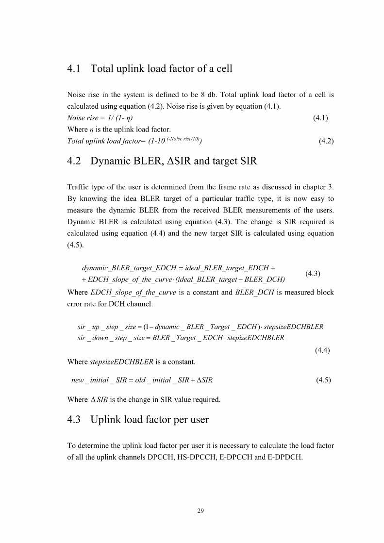
4.1 Total uplink load factor of a cell Noise rise in the system is defined to be 8 db. Total uplink load factor of a cell is calculated using equation (4.2). Noise rise is given by equation (4.1). Noise rise = 1/ (1- η) (4.1) Where η is the uplink load factor. Total uplink load factor= (1-10 (-Noise rise/10)) (4.2)

4.2 Dynamic BLER, ΔSIR and target SIR Traffic type of the user is determined from the frame rate as discussed in chapter 3. By knowing the idea BLER target of a particular traffic type, it is now easy to measure the dynamic BLER from the received BLER measurements of the users. Dynamic BLER is calculated using equation (4.3). The change is SIR required is calculated using equation (4.4) and the new target SIR is calculated using equation (4.5).

BLER_DCH)R_target(ideal_BLErve_of_the_cuEDCH_slopeCH_target_EDideal_BLEREDCHER_target_dynamic_BL

−⋅++=

(4.3)

Where EDCH_slope_of_the_curve is a constant and BLER_DCH is measured block error rate for DCH channel.

HBLERstepizeEDCEDCHTargetBLERsizestepdownsirCHBLERstepsizeEDEDCHTargetBLERdynamicsizestepupsir

⋅=⋅−=

_____)___1(___

(4.4) Where stepsizeEDCHBLER is a constant.

SIRSIRinitialoldSIRinitialnew ∆+= ____ (4.5)

Where ∆SIR is the change in SIR value required.

4.3 Uplink load factor per user To determine the uplink load factor per user it is necessary to calculate the load factor of all the uplink channels DPCCH, HS-DPCCH, E-DPCCH and E-DPDCH.

29

4.3.1 DPCCH load factor Load factor LDPCCH is calculated for the DPCCH overhead from the planned SIR target of the DPCCH using equation (4.6).

DPCCH

DPCCHDPCCH

SIRSF

L+

=1

1

(4.6)

Where SFDPCCH is the spreading factor of the UL DPCCH and SIRDPCCH is the value of the SIR target calculated from the equation (4.5).

Converting equation (4.6) into logarithmic scale yields equation (4.7).

LDPCCH = 10 ((SIR – 10log10 (SF))/10) (4.7)

Where SIR is expressed in db.

Considering low power offsets, equation (4.7) becomes equation (4.8).

LDPCCH = 10 ((SIR – 10log10 (SF) + DPCCH power offset)/10) (4.8)

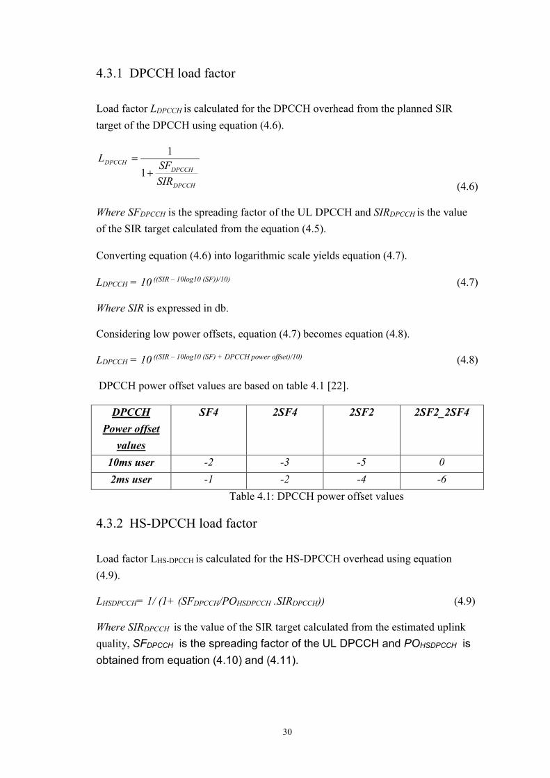
DPCCH power offset values are based on table 4.1 [22].

DPCCH Power offset

values

SF4 2SF4 2SF2 2SF2_2SF4

10ms user -2 -3 -5 0 2ms user -1 -2 -4 -6

Table 4.1: DPCCH power offset values

4.3.2 HS-DPCCH load factor

Load factor LHS-DPCCH is calculated for the HS-DPCCH overhead using equation (4.9).

LHSDPCCH= 1/ (1+ (SFDPCCH/POHSDPCCH .SIRDPCCH)) (4.9)

Where SIRDPCCH is the value of the SIR target calculated from the estimated uplink quality, SFDPCCH is the spreading factor of the UL DPCCH and POHSDPCCH is obtained from equation (4.10) and (4.11).

30

( )

⋅⋅

⋅⋅⋅=

2

c

hs

2

c

hs +-1sho

shoshononsho

nonshoshocqiHSDPCCH PPPPOββ

νββ

ν (4.10)

( )

( )shofbc,

shofbc,shorep,

nonshofbc,

nonshofbc,nonshorep,

CQI

CQI,CQI2minCQI

CQI,CQI2min

⋅=

⋅=

sho

nonsho

ν

ν

(4.11)

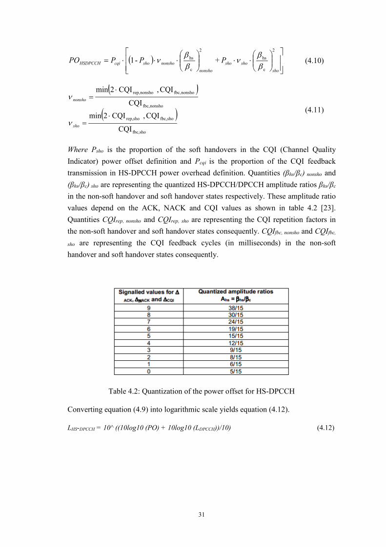
Where Psho is the proportion of the soft handovers in the CQI (Channel Quality Indicator) power offset definition and Pcqi is the proportion of the CQI feedback transmission in HS-DPCCH power overhead definition. Quantities (βhs/βc) nonsho and (βhs/βc) sho are representing the quantized HS-DPCCH/DPCCH amplitude ratios βhs/βc in the non-soft handover and soft handover states respectively. These amplitude ratio values depend on the ACK, NACK and CQI values as shown in table 4.2 [23]. Quantities CQIrep, nonsho and CQIrep, sho are representing the CQI repetition factors in the non-soft handover and soft handover states consequently. CQIfbc, nonsho and CQIfbc,

sho are representing the CQI feedback cycles (in milliseconds) in the non-soft handover and soft handover states consequently.

Table 4.2: Quantization of the power offset for HS-DPCCH

Converting equation (4.9) into logarithmic scale yields equation (4.12).

LHS-DPCCH = 10^ ((10log10 (PO) + 10log10 (LDPCCH))/10) (4.12)

31

4.3.3 E-DPCCH load factor Load factor LE-DPCCH is calculated for the E-DPCCH overhead using equation (4.13).

LE-DPCCH = LDPCCH . Aec2 (4.13)

Where Aec is the gain factor for E-DPCCH (βec)/ gain factor for DPCCH (βc)’.

Aec is the E-DPCCH power offset which is signalled by the higher layers as shown in table 4.3 [23].

Table 4.3: Quantization of the power offset for E-DPCCH

Converting equation (4.13) into logarithmic scale yields equation (4.14).

LE-DPCCH = 10 ((10log10 (LDPCCH) + 10log10 (Aec2))/10) (4.14)

4.3.4 E-DPDCH load factor Load factor E-DPDCH depends on the E-DCH transport bock size chosen by UE to transmit in uplink and the corresponding power offset required for this transmission. Scheduler in Node B and E-TFCI selection in UE is responsible for choosing the transport block size and defining the required power offset value. Load factor LE-

DPDCH is calculated for the E-DPDCH overhead using equation (4.15).

LE-DPDCH = LDPCCH . Absolute grant value (4.15) Absolute grant value = Aed . Number of codes (4.16)

Where Aed is the ’Gain factor for E-DPDCH (βed)/ gain factor for DPCCH (βc)’. Aed is the E-DPDCH power offset value which is signalled by the scheduler in Node B, in terms of absolute grants as shown in annexure 1. This value depends on the UE power headroom and E-DCH buffer status. All the index values from 2 to 31 are mapped to a certain power value that the UE can use for its transmission. Scheduling

32

grant is now mapped to the corresponding ETFCI values from the scheduler grant to ETFCI table and the ETFCI is mapped to the corresponding transport block size from the ETFCI to TB (Transport Block) size tables [24]. The values in the tables depend on the spreading factors used for data transmission and also on the transmission time interval. ETFCI to TB size mapping tables are shown in annexure 2 and scheduling grant to ETFCI mapping tables are shown in annexure 1.

For the purpose of simulation, MAC-d PDU (Packet Data Unit) size is fixed to 336 bits including both header and data part. In HSUPA, we consider that one transport block has only one MAC-e/ MAC-i PDU and each MAC-e/MAC-i PDU has one MAC-d flow in it. MAC-e or MAC-i PDU size is now determined using equation (4.17) and (4.18) respectively.

Total_bits_in_MACe = Number_of_MACes_PDUs . (DDI_size + TSN_size +

Num_MACd_PDUs_size + (Total_bits_in_MAC_d . Number_of_MACd_PDUs)) (4.17)

Where DDI_size indicates the logical channel id, MAC-d flow id and size of the MAC-d PDU's concatenated into the associated MAC-es PDU, TSN_size indicates the transmission sequence number of MAC-es PDU’s, Num_MACd_PDUs_size indicates the size for number of MAC-d PDU's identifier and Number_of_MACd_PDUs indicates the number of consecutive MAC-d PDU's in one MAC-es PDU.

Total_bits_in_MACi=Number_of_MACes_PDUs.(Si+TSNi) +Number_of_MACd_PDUs . (LCHIDi+Li+Fi+Total_bits_in_MAC_d) (4.18)

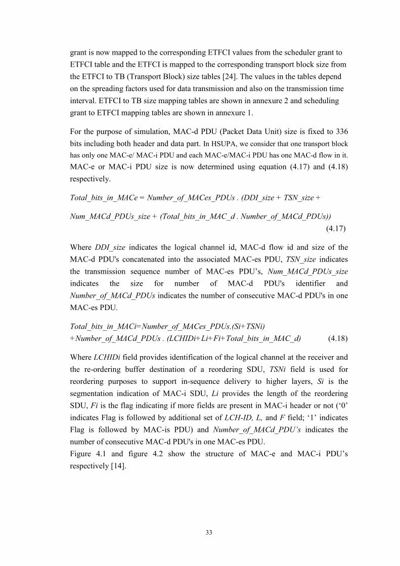
Where LCHIDi field provides identification of the logical channel at the receiver and the re-ordering buffer destination of a reordering SDU, TSNi field is used for reordering purposes to support in-sequence delivery to higher layers, Si is the segmentation indication of MAC-i SDU, Li provides the length of the reordering SDU, Fi is the flag indicating if more fields are present in MAC-i header or not (‘0’ indicates Flag is followed by additional set of LCH-ID, L, and F field; ‘1’ indicates Flag is followed by MAC-is PDU) and Number_of_MACd_PDU’s indicates the number of consecutive MAC-d PDU's in one MAC-es PDU. Figure 4.1 and figure 4.2 show the structure of MAC-e and MAC-i PDU’s respectively [14].

33

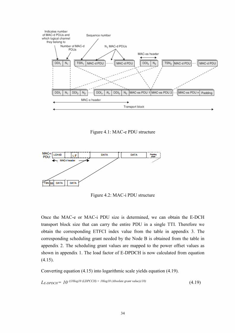
Figure 4.1: MAC-e PDU structure

Figure 4.2: MAC-i PDU structure

Once the MAC-e or MAC-i PDU size is determined, we can obtain the E-DCH transport block size that can carry the entire PDU in a single TTI. Therefore we obtain the corresponding ETFCI index value from the table in appendix 3. The corresponding scheduling grant needed by the Node B is obtained from the table in appendix 2. The scheduling grant values are mapped to the power offset values as shown in appendix 1. The load factor of E-DPDCH is now calculated from equation (4.15).

Converting equation (4.15) into logarithmic scale yields equation (4.19).

LE-DPDCH = 10 ((10log10 (LDPCCH) + 10log10 (Absolute grant value))/10) (4.19)

34

4.3.5 Load factor per user

Load factor depends on the duration of time the UE was transmitting in uplink and also on the target SIR required to achieve quality transmission. It is given by equation (4.20). Total load per user = (1+i) . (LDPCCH + LHSDPCCH + Activity factor . (LE-DPCCH + LE-

DPDCH)) (4.20)

Where i is the interference factor from other cells and is equal to 0.5, Activity factor is calculated in next section and LDPCCH, LHSDPCCH, LE-DPCCH and LE-DPDCH are already calculated above.

4.4 Activity factor of users

Considering all the users in a cell are similar with respect to spreading factors used, modulation used, transport block sizes used etc and also considering all the users are scheduled on a round robin approach, the activity factor of each user varies depending on the target SIR required for that particular user. It is calculated according to equation (4.21).

Activity factor (k) = ((Total uplink load factor/number of users) . (1/ (1+i)) - LDPCCH (k) + LHSDPCCH (k))/ (LE-DPCCH (k) + LE-DPDCH (k)) (4.21)

Where k indicates the kth user in the cell.

4.5 Average user throughput and cell throughput Once the activity factors of all HSUPA users are known and by considering a fixed radio bearer bit rate, average user throughput and cell throughput are determined using equation (4.22) and (4.23) respectively.

Average user throughput (number of users) = (Sum (Activity factors of all the users) . Bit rate of radio bearer)/number of users (4.22)

35

Cell throughput (number of users) = Average throughput (number of users) . number of users (4.23)

Where Bit rate of radio bearer is either 32Kbps or 64Kbps.

36

Chapter 5

Analysis and simulation results

To understand the benefits of ‘Dynamic BLER feature’ we simulate 3 scenarios with 10ms TTI users and 2ms TTI users and then analyze the results. In the first scenario, we consider 10 HSUPA users. In the second scenario, we consider 1 HSUPA user. In the third scenario, we consider 72 HSUPA users.

5.1 With 10 HSUPA users in the cell In this section, the cell throughput is first calculated without the feature being activated (Ideal BLER target = 10%). Next, the cell throughput is calculated with the feature activated (different ideal BLER target values based on the traffic types). The analysis is done for both 10ms and 2ms users. The results are then compared and analyzed.

5.1.1 Total uplink load factor Since the noise rise target of the cell is 8 db, total uplink load factor is equal to 84.15% calculated using equation (4.2).

5.1.2 Dynamic BLER, ΔSIR and target SIR Let us consider we have 10 users within a cell. The estimated BLER values and frame rate for all the 10 users based on the Nokia Networks system test logs are shown in table 5.1. Also shown in the table is the target SIR calculated with and without the feature. Dynamic BLER, ΔSIR and target SIR are measured using equation (4.3), (4.4) and (4.5) respectively.

37

User number

Estimated BLER value

Frame rate Traffic types

Target SIR (without feature)

Target SIR (With feature)

1 0.3 >10(10ms),50(2ms) Continuous 5.6 2.4 2 0.27 >10(10ms),50(2ms) Continuous 5.48 2.46 3 0.25 <10(10ms),50(2ms) Bursty 5.4 5.4 4 0.22 <10(10ms),50(2ms) Bursty 5.28 5.28 5 0.21 >10(10ms),50(2ms) Continuous 5.24 2.58 6 0.19 <10(10ms),50(2ms) Bursty 5.16 5.16 7 0.16 >10(10ms),50(2ms) Continuous 5.04 2.68 8 0.15 <10(10ms),50(2ms) Bursty 5 5 9 0.14 >10(10ms),50(2ms) Continuous 4.96 2.72 10 0.10 <10(10ms),50(2ms) Bursty 4.8 4.8

Table 5.1: BLER to SIR mapping From table 5.1, we observe the difference in target SIR with and without the feature. This results in significant reduction of uplink interference caused by the user transmissions.

5.1.3 Load factor of uplink channels Load factors of DPCCH, HS-DPCCH, E-DPCCH and E-DPDCH are shown in table 5.2 and 5.3 that are calculated based on equations (4.8), (4.12), (4.14) and (4.19) respectively without and with the feature. To calculate the load factor of HS-DPCCH and E-DPCCH quantized amplitude ratios were considered based on the signalled values depending on 10ms or 2ms users. To calculate the E-DCH TB size, MAC-d PDU size of 336 bits is considered. E-DCH TB size varies depending on 10ms and 2ms users and is calculated using equation (4.17) and (4.18).

38

User number

LDPCCH

(10ms/2ms) LHSDPCCH

(10ms/2ms) LE-DPCCH

(10ms/2ms) LE-DPDCH

(10ms/2ms) 1 0.448/0.356 0.244/0.193 0.287/0.912 1.793/4.446 2 0.436/0.346 0.237/0.188 0.279/0.887 1.745/4.324 3 0.428/0.340 0.233/0.185 0.274/0.870 1.713/4.245 4 0.416/0.330 0.226/0.180 0.266/0.847 1.666/4.130 5 0.412/0.327 0.224/0.178 0.264/0.839 1.651/4.092 6 0.405/0.321 0.220/0.175 0.259/0.824 1.621/4.017 7 0.394/0.313 0.214/0.170 0.252/0.801 1.576/3.908 8 0.390/0.310 0.212/0.168 0.250/0.794 1.562/3.872 9 0.387/0.307 0.210/0.167 0.247/0.787 1.548/3.836 10 0.373/0.296 0.202/0.161 0.238/0.758 1.492/3.698

Table 5.2: Load factors of channels (without feature)

User number

LDPCCH

(10ms/2ms) LHSDPCCH

(10ms/2ms) LE-DPCCH

(10ms/2ms) LE-DPDCH

(10ms/2ms) 1 0.214/0.170 0.116/0.092 0.137/0.436 0.858/2.128 2 0.217/0.172 0.118/0.094 0.139/0.442 0.870/2.157 3 0.428/0.340 0.233/0.185 0.274/0.870 1.713/4.245 4 0.416/0.330 0.226/0.180 0.266/0.847 1.666/4.130 5 0.223/0.177 0.121/0.096 0.143/0.454 0.894/2.218 6 0.405/0.321 0.220/0.175 0.259/0.824 1.621/4.017 7 0.228/0.181 0.124/0.098 0.146/0.465 0.915/2.269 8 0.390/0.310 0.212/0.168 0.250/0.794 1.562/3.872 9 0.231/0.183 0.125/0.099 0.147/0.468 0.924/2.290 10 0.373/0.296 0.202/0.161 0.238/0.758 1.492/3.698

Table 5.3: Load factors of channels (with feature)

5.1.4 Average user throughput and cell throughput Average user throughput with 10 users in the cell improved from 84 Kbps to 124 Kbps in case of 10ms users and it improved from 167 Kbps to 245 Kbps in case of 2ms users. Therefore, cell throughput also increased from 841 Kbps to 1.24 Mbps in case of 10ms users and it increased from 1.67 Mbps to 2.45 Mbps in case of 2ms users. Interference factor of 0.5 is considered for the calculations. The plots for cell throughput are shown in figure 5.1 and 5.2 for 10 ms users and in figure 5.3 and 5.4

39

for 2ms users.

Figure 5.1: Cell throughput with 10 10ms users (HSUPA Dynamic BLER Feature

inactive)

Figure 5.2: Cell throughput with 10 10ms users (HSUPA Dynamic BLER Feature active)

Figure 5.1 and 5.2 shows the variation of cell throughput with respect to the number of users within the cell. All the users are of same type i.e. 10ms TTI, 32Kbps bearer bit rate and spreading factor 2SF2. As the number of users increase in the cell, the cell throughput decreases due to the increase in interference. By comparing figure 5.1 and 5.2, we observe the improvement in cell throughput by about 400 Kbps with 10 users when the feature is active.

40

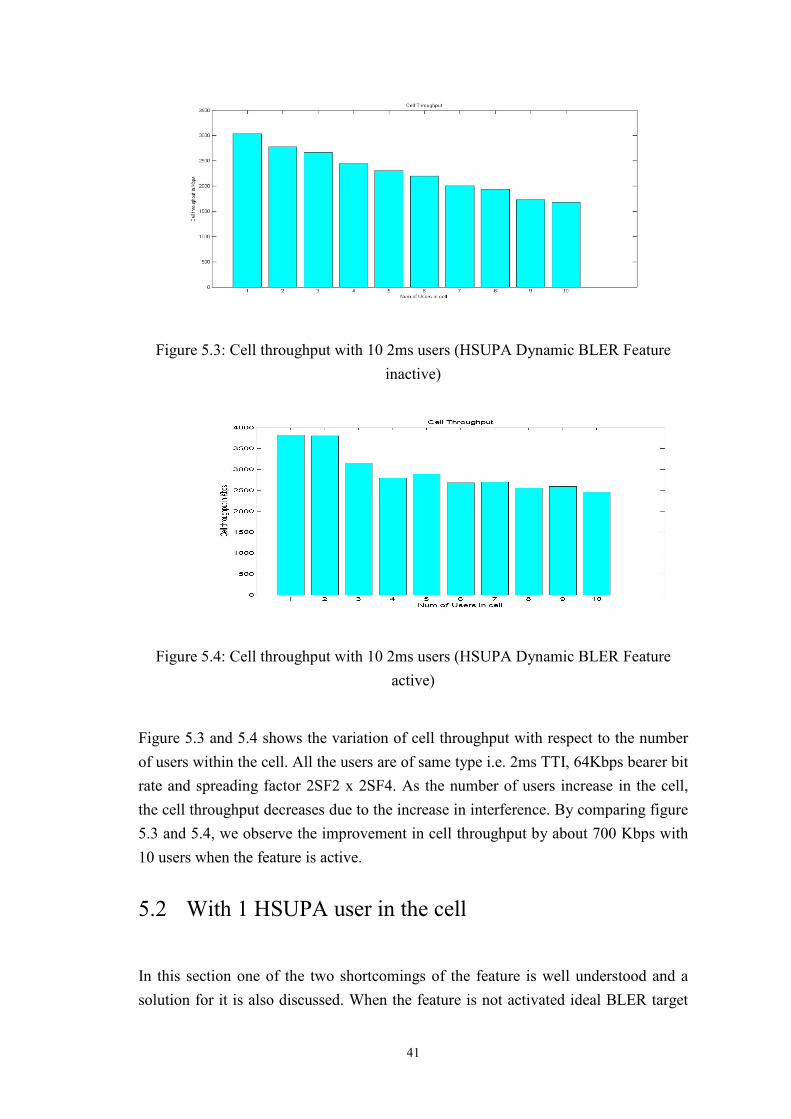
Figure 5.3: Cell throughput with 10 2ms users (HSUPA Dynamic BLER Feature inactive)

Figure 5.4: Cell throughput with 10 2ms users (HSUPA Dynamic BLER Feature active)

Figure 5.3 and 5.4 shows the variation of cell throughput with respect to the number of users within the cell. All the users are of same type i.e. 2ms TTI, 64Kbps bearer bit rate and spreading factor 2SF2 x 2SF4. As the number of users increase in the cell, the cell throughput decreases due to the increase in interference. By comparing figure 5.3 and 5.4, we observe the improvement in cell throughput by about 700 Kbps with 10 users when the feature is active.

5.2 With 1 HSUPA user in the cell

In this section one of the two shortcomings of the feature is well understood and a solution for it is also discussed. When the feature is not activated ideal BLER target

41

values of 10% is used to calculate target SIR value, but when the feature is activated and say the user is of continuous traffic type, ideal BLER target value of 31.6% is used. Higher ideal BLER target value results in higher HARQ retransmissions and also increases the probability of RLC retransmissions [25]. All these factors result in the increase of TCP round trip time (delay in TCP ACK) and thus reduces the end to end TCP throughput in downlink [26]. A simple simulator is implemented to show the effect of increase in ideal BLER target values on TCP round trip time and thus on end to end TCP throughput. The implementation is explained in this section along with the simulation results.

Consider a TCP segment size both in uplink and downlink. Calculate the number of HARQ packets needed to transmit this TCP segment using equation (5.1) and (5.2) [26].

Number_of_HARQ_Packets_UL=ceil (SS_UL/MAC_E_PDU_size_UL) (5.1)

Number_of_HARQ_Packets_DL=ceil (SS_DL/MAC_E_PDU_size_DL) (5.2)

Where SS_UL is the TCP segment size in uplink and SS_DL is the TCP segment size in downlink.

Now determine the number of HARQ packets that require one, two and three retransmissions using equation (5.3), (5.4) and (5.5) respectively [27].

Pb_1RX= (1-(1-BLER_1TX) (BLER_1TX_UL^1 . Number_of_HARQ_Packets)) (5.3)

Pb_2RX= (1-(1-BLER_2TX) (BLER_2TX_UL. ^2 . Number_of_HARQ_Packets)) (5.4)

Pb_3RX= (1-(1-BLER_3TX) (BLER_3TX_UL. ^3 . Number_of_HARQ_Packets)) (5.5)

Where Pb_1RX is the probability of HARQ packets that require one retransmission, Pb_2RX is the probability of HARQ packets that require two retransmissions, Pb_3RX is the probability of HARQ packets that require three retransmissions, BLER_1TX is the measured BLER after one retransmission, BLER_2TX is the measured BLER after two retransmissions and BLER_3TX is the measured BLER after three retransmissions.

Let us now consider that a TCP ACK is sent for every two TCP segments successfully transmitted. Therefore, HARQ round trip time can be determined using equation (5.6) and it varies depending on 10ms and 2ms users [26].

42

RTT_HARQ=Num_TCP_segments_UL_per_round.(Number_of_HARQ_Packets_UL.HARQ_TX+Number_of_HARQ_Packets_UL.Pb_1RX_UL.HARQ_RX+Number_of_HARQ_Packets_UL.Pb_2RX_UL.2.HARQ_RX+Number_of_HARQ_Packets_UL.Pb_3RX_UL.3.HARQ_RX)+Num_TCP_segments_DL_per_round.(Number_of_HARQ_Packets_DL.HARQ_TX+Number_of_HARQ_Packets_DL.Pb_1RX_DL.HARQ_RX+Number_of_HARQ_Packets_DL.Pb_2RX_DL.2.HARQ_RX+Number_of_HARQ_Packets_DL.Pb_3RX_DL.3.HARQ_RX) (5.6)

Where RTT_HARQ is the HARQ round trip time, Num_TCP_segments_UL_per_round is equal to 1, Num_TCP_segments_DL_per_round is equal to 2 (One TCP ACK in uplink for 2 TCP segments in downlink), HARQ_TX is the frame length in millisecond and HARQ_RX is the HARQ retransmission time in millisecond.

TCP round trip time can now be calculated using equation (5.7) [26].

RTT_TCP=2.RTT_wire+RTT_HARQ+(2.Number_of_HARQ_Packets_DL.(1+Pb_1RX_DL+Pb_2RX_DL+Pb_3RX_DL)+Number_of_HARQ_Packets_UL.(1+Pb_1RX_UL+Pb_2RX_UL+Pb_3RX_UL)).D_HARQ (5.7)

Where RTT_TCP is the TCP round trip time, RTT_wire is the delay caused in wired transmission part of the network and D_HARQ is the fixed component delay to process one HARQ frame.

Finally, TCP throughput is calculated using equation (5.8).

TCP_throughput=TCP_cong_win_bits/ (RTT_TCP/1000) (5.8)

Where TCP_cong_win_bits is the TCP congestion window size in bits.

43

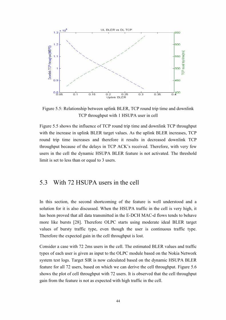
Figure 5.5: Relationship between uplink BLER, TCP round trip time and downlink TCP throughput with 1 HSUPA user in cell

Figure 5.5 shows the influence of TCP round trip time and downlink TCP throughput with the increase in uplink BLER target values. As the uplink BLER increases, TCP round trip time increases and therefore it results in decreased downlink TCP throughput because of the delays in TCP ACK’s received. Therefore, with very few users in the cell the dynamic HSUPA BLER feature is not activated. The threshold limit is set to less than or equal to 3 users.

5.3 With 72 HSUPA users in the cell

In this section, the second shortcoming of the feature is well understood and a solution for it is also discussed. When the HSUPA traffic in the cell is very high, it has been proved that all data transmitted in the E-DCH MAC-d flows tends to behave more like bursts [28]. Therefore OLPC starts using moderate ideal BLER target values of bursty traffic type, even though the user is continuous traffic type. Therefore the expected gain in the cell throughput is lost.

Consider a case with 72 2ms users in the cell. The estimated BLER values and traffic types of each user is given as input to the OLPC module based on the Nokia Network system test logs. Target SIR is now calculated based on the dynamic HSUPA BLER feature for all 72 users, based on which we can derive the cell throughput. Figure 5.6 shows the plot of cell throughput with 72 users. It is observed that the cell throughput gain from the feature is not as expected with high traffic in the cell.

44

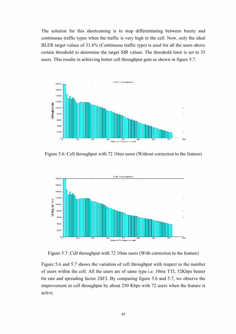
The solution for this shortcoming is to stop differentiating between bursty and continuous traffic types when the traffic is very high in the cell. Now, only the ideal BLER target values of 31.6% (Continuous traffic type) is used for all the users above certain threshold to determine the target SIR values. The threshold limit is set to 35 users. This results in achieving better cell throughput gain as shown in figure 5.7.

Figure 5.6: Cell throughput with 72 10ms users (Without correction to the feature)

Figure 5.7: Cell throughput with 72 10ms users (With correction to the feature)

Figure 5.6 and 5.7 shows the variation of cell throughput with respect to the number of users within the cell. All the users are of same type i.e. 10ms TTI, 32Kbps bearer bit rate and spreading factor 2SF2. By comparing figure 5.6 and 5.7, we observe the improvement in cell throughput by about 250 Kbps with 72 users when the feature is active.

45

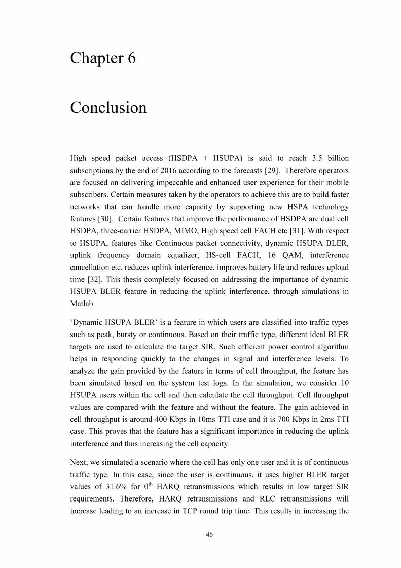
Chapter 6

Conclusion

High speed packet access (HSDPA + HSUPA) is said to reach 3.5 billion subscriptions by the end of 2016 according to the forecasts [29]. Therefore operators are focused on delivering impeccable and enhanced user experience for their mobile subscribers. Certain measures taken by the operators to achieve this are to build faster networks that can handle more capacity by supporting new HSPA technology features [30]. Certain features that improve the performance of HSDPA are dual cell HSDPA, three-carrier HSDPA, MIMO, High speed cell FACH etc [31]. With respect to HSUPA, features like Continuous packet connectivity, dynamic HSUPA BLER, uplink frequency domain equalizer, HS-cell FACH, 16 QAM, interference cancellation etc. reduces uplink interference, improves battery life and reduces upload time [32]. This thesis completely focused on addressing the importance of dynamic HSUPA BLER feature in reducing the uplink interference, through simulations in Matlab.

‘Dynamic HSUPA BLER’ is a feature in which users are classified into traffic types such as peak, bursty or continuous. Based on their traffic type, different ideal BLER targets are used to calculate the target SIR. Such efficient power control algorithm helps in responding quickly to the changes in signal and interference levels. To analyze the gain provided by the feature in terms of cell throughput, the feature has been simulated based on the system test logs. In the simulation, we consider 10 HSUPA users within the cell and then calculate the cell throughput. Cell throughput values are compared with the feature and without the feature. The gain achieved in cell throughput is around 400 Kbps in 10ms TTI case and it is 700 Kbps in 2ms TTI case. This proves that the feature has a significant importance in reducing the uplink interference and thus increasing the cell capacity.

Next, we simulated a scenario where the cell has only one user and it is of continuous traffic type. In this case, since the user is continuous, it uses higher BLER target values of 31.6% for 0th HARQ retransmissions which results in low target SIR requirements. Therefore, HARQ retransmissions and RLC retransmissions will increase leading to an increase in TCP round trip time. This results in increasing the

46

delay of TCP ACK in uplink and thus reduces the end to end TCP downlink throughput. The simulation shows that as the BLER values increase from 0.15 to 0.30, the TCP round trip time increases from 450ms to 600ms and thus reduces the TCP downlink throughput. The solution provided for this was to deactivate the feature when the number of HSUPA users within the cell is less than 3. This is one of the important factors to be considered with respect to this feature.

Finally, we simulated a scenario with 72 users of different traffic types within the cell. The observation was that once the number of users in the cell reaches a certain limit (say 35), the continuous traffic type are seen as bursty traffic type and hence moderate BLER targets of 10% are used instead of 31.6%. This results in the reduction of cell throughput significantly it was measured as 200 Kbps with 72 users in the cell. The solution for this was to stop differentiating the users into bursty and continuous traffic types and just using BLER targets of 31.6% after 35 users in the cell. The cell throughput achieved based on this was 450 Kbps with 72 users. So, we see a significant gain in cell throughput.

Once we consider both the problems of Dynamic HSUPA BLER feature by using proper solutions, this feature provides enhancement in cell capacity and cell coverage as proved from the simulation results.

47

References

[1] Pankaj Sharma, “Evolution of Mobile Wireless Communication Networks-1G to 5G as well as Future Prospective of Next Generation Communication Network”, IJCSMC journal, Vol.2, Issue 8, 2013, pp. 47-53.

[2] Ericsson, “Ericsson mobility report on the pulse of the networked society”, 2012.

[3] Dimitri Konstantas, Val Jones, Richard Bults, “MobiHealth – innovative 2.5/3G mobile services and applications for healthcare”, University of Twente, Center for Telematics and Information Technology – APS.

[4] Nomor Research, White Paper – Dual Cell HSDPA and its Future Evolution, 2009.

[5] Roman Maslennikov, “Evaluation of MIMO Transmission for HSUPA”, Vehicular technology conference IEEE 75th, pp. 1-5, 2012.

[6] Tektronix, “HSDPA protocols and resource allocations” version E003, pp. 4-9.

[7] Motorola, White paper-High speed uplink packet access, 2007.

[8] Messaoud Eljamai, “3GPP Enhanced Uplink UMTS Simulation Description and Environment”, International journal of Science and Technology, volume 2 No. 10, 2012.

[9] Nokia Networks, “RAN 2302 EFS”, 2013.

[10] 3GPP, http://www.3gpp.org/about-3gpp

[11] H. Holma and A. Toskala, HSDPA/HSUPA for UMTS: High speed radio access for mobile communications, John Wiley & Sons, 2006. [12] 3GPP, “Radio Interface Protocol Architecture (Release 6)”, TS 25.301, 2005-09.

[13] Chris Johnson, Radio Access Networks for UMTS: Principles and practice, John Wiley & Sons, 2008. [14] 3GPP, “Radio Medium Access Control (MAC) protocol specification (Release 9)”, TS 25.321, 2010-06.

[15] Ajay R. Mishra, Cellular technologies for emerging markets 2G, 3G and beyond, John Wiley & Sons, 2010. [16] Nokia Networks, “OLPC functional description”, Release RN7.0.

48

[17] S Nourizadeh, P Taaghol, R Tafazolli, “A novel closed loop power control for UMTS”, 3G Mobile Communication Technologies, 2000. First International Conference, pp 56, Mar 2009. [18] Nokia Networks, ‘Point. Shoot. Upload. Software upgrades for a picture perfect experience’,http://blog.networks.nokia.com/mobile-networks/2013/11/20/point-shoot-upload-software-upgrades-for-a-picture-perfect-experience/ ,2013. [19] Meng Zhang, “Throughput-based and Power-based Load Control in HSUPA”, IEEE, Vol 2, pp. 969-973, 2005. [20] Nokia Networks, “Admission Control functional description”, Release RN6.0.

[21] Nokia Networks, “HSUPA RRM in RNC functional description”, Release RN7.0.

[22] 3GPP, “Physical layer procedures (FDD)”, TS 25.214, 1999.

[23] ETSI, “Universal Mobile Telecommunications System (UMTS); Spreading and modulation (FDD)”, TS 125.213. Version 7.2.0, 2007-05.

[24] Chen Tao, “Effect of Node-B Scheduling Algorithms on High Speed Uplink

Packet Access with E-TFC Selection”, Nokia Research Centre, 2006.

[25] Massimo Bertinelli, “WCDMA Enhanced uplink: HSUPA link level performance study”, IEEE 16th International Symposium, 2005.

[26] Janne Peisa, “Analytical Model for TCP file transfers over UMTS”, Ericsson Research.

[27] http://rfmw.em.keysight.com/wireless/helpfiles/opt419/1._hsupa_uplink.htm

[28] Pekka Kohonen, “TS-RNC-SW-189-I5”, Nokia Networks.

[29] Ericsson, “Ericsson mobility report on the pulse of the networked society”, 2013.

[30] Nokia Networks, “New software boosts WCDMA network capacity and performance”, Newsletter, 2013.

[31] Nokia Networks, http://networks.nokia.com/news-events/insight-newsletter/articles/how-hspa-is-changing-to-stay-ahead-in-mobile-broadband, 2012.

[32] Nokia Networks, “Taking HSPA to the next level with Release 12 and beyond”, white paper, 2014.

49

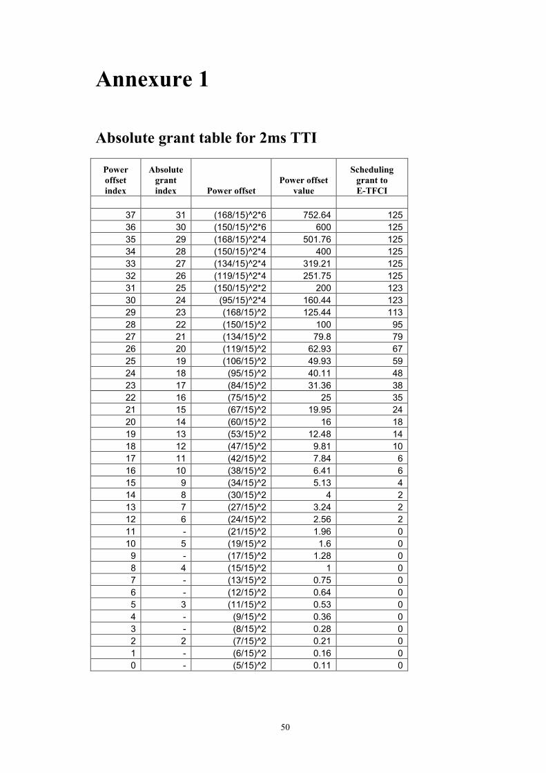
Annexure 1

Absolute grant table for 2ms TTI

Power offset index

Absolute grant index Power offset

Power offset value

Scheduling grant to E-TFCI

37 31 (168/15)^2*6 752.64 125 36 30 (150/15)^2*6 600 125 35 29 (168/15)^2*4 501.76 125 34 28 (150/15)^2*4 400 125 33 27 (134/15)^2*4 319.21 125 32 26 (119/15)^2*4 251.75 125 31 25 (150/15)^2*2 200 123 30 24 (95/15)^2*4 160.44 123 29 23 (168/15)^2 125.44 113 28 22 (150/15)^2 100 95 27 21 (134/15)^2 79.8 79 26 20 (119/15)^2 62.93 67 25 19 (106/15)^2 49.93 59 24 18 (95/15)^2 40.11 48 23 17 (84/15)^2 31.36 38 22 16 (75/15)^2 25 35 21 15 (67/15)^2 19.95 24 20 14 (60/15)^2 16 18 19 13 (53/15)^2 12.48 14 18 12 (47/15)^2 9.81 10 17 11 (42/15)^2 7.84 6 16 10 (38/15)^2 6.41 6 15 9 (34/15)^2 5.13 4 14 8 (30/15)^2 4 2 13 7 (27/15)^2 3.24 2 12 6 (24/15)^2 2.56 2 11 - (21/15)^2 1.96 0 10 5 (19/15)^2 1.6 0

9 - (17/15)^2 1.28 0 8 4 (15/15)^2 1 0 7 - (13/15)^2 0.75 0 6 - (12/15)^2 0.64 0 5 3 (11/15)^2 0.53 0 4 - (9/15)^2 0.36 0 3 - (8/15)^2 0.28 0 2 2 (7/15)^2 0.21 0 1 - (6/15)^2 0.16 0 0 - (5/15)^2 0.11 0

50

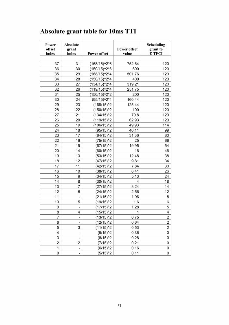
Absolute grant table for 10ms TTI

Power offset index

Absolute grant index Power offset

Power offset value

Scheduling grant to E-TFCI

37 31 (168/15)^2*6 752.64 120 36 30 (150/15)^2*6 600 120 35 29 (168/15)^2*4 501.76 120 34 28 (150/15)^2*4 400 120 33 27 (134/15)^2*4 319.21 120 32 26 (119/15)^2*4 251.75 120 31 25 (150/15)^2*2 200 120 30 24 (95/15)^2*4 160.44 120 29 23 (168/15)^2 125.44 120 28 22 (150/15)^2 100 120 27 21 (134/15)^2 79.8 120 26 20 (119/15)^2 62.93 120 25 19 (106/15)^2 49.93 114 24 18 (95/15)^2 40.11 99 23 17 (84/15)^2 31.36 80 22 16 (75/15)^2 25 66 21 15 (67/15)^2 19.95 54 20 14 (60/15)^2 16 46 19 13 (53/15)^2 12.48 38 18 12 (47/15)^2 9.81 34 17 11 (42/15)^2 7.84 30 16 10 (38/15)^2 6.41 26 15 9 (34/15)^2 5.13 24 14 8 (30/15)^2 4 18 13 7 (27/15)^2 3.24 14 12 6 (24/15)^2 2.56 12 11 - (21/15)^2 1.96 8 10 5 (19/15)^2 1.6 6

9 - (17/15)^2 1.28 5 8 4 (15/15)^2 1 4 7 - (13/15)^2 0.75 2 6 - (12/15)^2 0.64 2 5 3 (11/15)^2 0.53 2 4 - (9/15)^2 0.36 0 3 - (8/15)^2 0.28 0 2 2 (7/15)^2 0.21 0 1 - (6/15)^2 0.16 0 0 - (5/15)^2 0.11 0

51

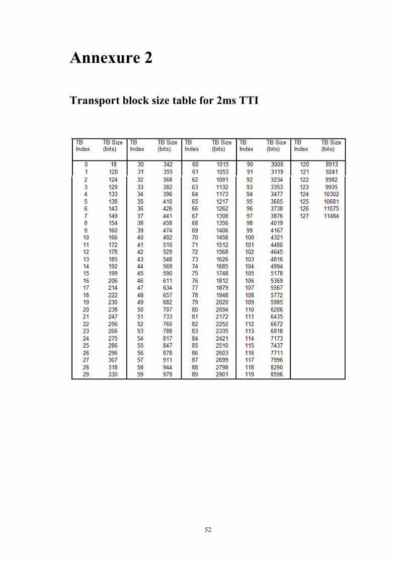
Annexure 2

Transport block size table for 2ms TTI

52

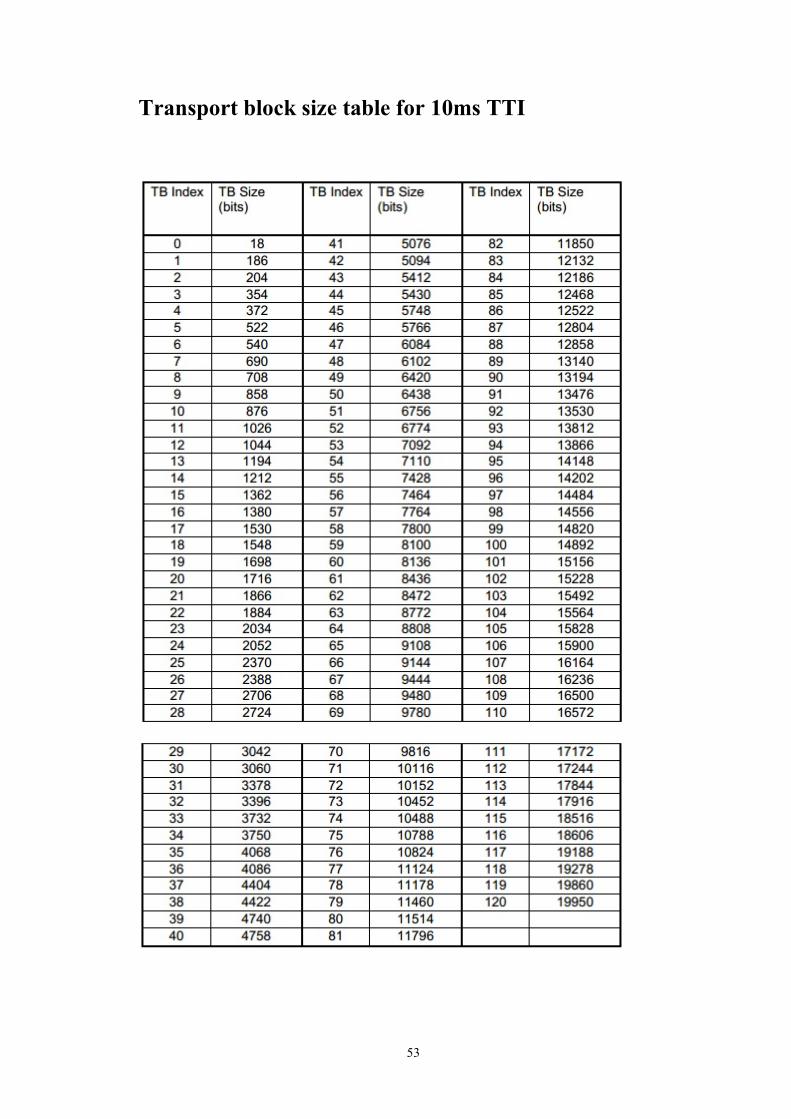
Transport block size table for 10ms TTI

53