HAL Id: hal-00519805https://hal.archives-ouvertes.fr/hal-00519805

Submitted on 21 Sep 2010

HAL is a multi-disciplinary open accessarchive for the deposit and dissemination of sci-entific research documents, whether they are pub-lished or not. The documents may come fromteaching and research institutions in France orabroad, or from public or private research centers.

L’archive ouverte pluridisciplinaire HAL, estdestinée au dépôt et à la diffusion de documentsscientifiques de niveau recherche, publiés ou non,émanant des établissements d’enseignement et derecherche français ou étrangers, des laboratoirespublics ou privés.

Performance-Based Reactive Navigation forNonholonomic Mobile Robots

Michael Defoort, Jorge Palos, Annemarie Kökösy, Thierry Floquet, WilfridPerruquetti

To cite this version:Michael Defoort, Jorge Palos, Annemarie Kökösy, Thierry Floquet, Wilfrid Perruquetti. Performance-Based Reactive Navigation for Nonholonomic Mobile Robots. Robotica, Cambridge University Press,2009, 27 (2), pp.281-290. <10.1017/S0263574708004700>. <hal-00519805>

Performance–Based Reactive Navigation forNonholonomic Mobile Robots∗

Michael Defoort1†, Jorge Palos2, Annemarie Kokosy2,Thierry Floquet1 and Wilfrid Perruquetti1

1LAGIS UMR CNRS 8146, Ecole Centrale de Lille,BP 48, Cite Scientifique, 59651 Villeneuve-d’Ascq, FRANCE

2ISEN, 41 bvd Vauban, 59 046 Lille Cedex, FRANCE

Abstract

This paper presents an architecture for the navigation of an autonomous mo-bile robot evolving in environments with obstacles. Instead of addressing motionplanning and control in different contexts, these issues are described in connectedmodules with performance requirement considerations. The planning problem isformulated as a constrained receding horizon planning problem and is solved inreal time with an efficient computational method that combines nonlinear controltheory, B-spline basis function and nonlinear programming. An integral slidingmode controller is used for trajectory tracking. Closed-loop stability of the track-ing errors is guaranteed in spite of unknown disturbances. It is also shown thatthis strategy is particularly useful if integral sliding mode control is combined withother methods to further robustify against perturbations. The effectiveness, perfectperformance of obstacle avoidance, real time and high robustness properties aredemonstrated by experimental results.

Keywords: Nonholonomic mobile robots, Reactive navigation, Receding horizon plan-ning, Sliding mode control.

1 Introduction

Wheeled mobile robots (WMRs) have been widely studied in the last two decades dueto their practical importance and theoretically interesting properties. Indeed, there areconsiderable research efforts toward solving mobile robot navigation in different appli-cations in indoor and outdoor environments (see [1, 2] and the survey paper [3]). For

∗This work was partially supported by the Region Nord Pas-de-Calais and the FEDER (European Fundsof Regional Development) under InterregACOS, the ARCIR Robocoopand theAUTORIS-TAT T31project.

†Corresponding author. E-mail: michael.defoort@ec-lille.fr

1

some navigation tasks like planetary exploration, robots are required to travel long dis-tances within constrained resources (energy, time. . . ). In such cases, efficient motionplanning and control algorithms are needed in order to achieve the goal while meetingcertain performance issue, such as geometric-based or time-based criteria.

Although motion planning and control are closely related in the robot navigationproblem, they are usually addressed as two separate problems in much of the exist-ing literature. Motion planning consists in generating a collision-free trajectory fromthe initial to the final desired positions and control is the determination of the physi-cal inputs to the robot motion components. These two problems are typically solvedusing methods from different areas such as those in artificial intelligence and controltheory. Such a separation makes it difficult to address robot performance in a completeapplication, since the planned trajectory may not be efficiently tracked. This fact canimply that the meaning of optimization in each step is lost. For instance, in a typicaltime optimal trajectory planning, the open-loop control schemes result in bang-bangor bang-singular-bang controls [4]. However, the discontinuities of the planned open-loop control may not produce a satisfactory path tracking result in practice and willnot be applicable to high speed traveling. In this research, we bridge the gap betweentrajectory planning and motion control.

Many theoretically challenging properties stem from the so-called nonholonomicconstraints imposed by the rolling wheels. A survey of nonholonomic control prob-lems can be found in [5]. Obstacles to the tracking of nonholonomic systems are theuncontrollability of their linear approximation and the fact that the Brockett’s necessarycondition to the existence of a smooth time-invariant state feedback is not satisfied [6].To overcome these difficulties, various methods have been investigated: homogeneousand time-varying feedbacks [7, 8], sinusoidal and polynomial controls [9], piecewisecontinuous controls [10], backstepping approaches [11] or discontinuous controls [12].However, most of these methods do not provide both fast convergence and good ro-bustness properties. Most of the control laws ensuring exponential or finite time con-vergence [13] are known to be non-robust under disturbances or modeling errors. Onthe other hand, control design methodologies like smooth time varying feedback [8],are quite insensitive to perturbations but imply a slow convergence.

In this paper, we propose a practical scheme for real time motion planning and con-trol of nonholonomic mobile robot moving in an uncertain environment. As illustratedin Fig. 1, the scheme consists of two main parts: (i) a real time collision-free motionplanner; (ii) a trajectory tracking controller. For each module, we explicitly addressthe performance considerations. In implementation, the motion planner dynamicallygenerates the optimal trajectory while the robot runs. High precision motion trackingis achieved by the combination of integral sliding mode control and time varying statefeedback. The main results are general and can be applied whenever integral slidingmode control is combined with other techniques to further robustify against distur-bances. Experimentations support the validity of the theoretical analysis and show thatthe performance of a time varying state feedback controller can be increased by thisparticular strategy.

The outline of this paper is as follows. In Section 2, the navigation problem is de-fined and the robot’s nonholonomic model is described. Motion planning is discussedin Section 3. Trajectory tracking strategy is presented in Section 4. Finally, in Section

2

�

��������

������

������

�����

�������

����

���������

�����������

��������

�������

�������

������������

����������

������

��������������������

���������� �!�

� �

������������������

Figure 1: Block diagram for navigation of a nonholonomic mobile robot with a motionplanner and a sliding mode controller.

5, we present the integration of the different modules and the experimental results on amobile robot.

2 Problem statement

2.1 Modeling of mobile robot

The mobile robot, shown in Fig. 2, is of unicycle-type. The robot body is of symmetricshape and the centre of mass is at the geometric centreC of the body. It has two drivingwheels fixed to the axis which passes throughC and one passive centrered orientablewheel. The two fixed wheels of radiusr, separated by2R, are independently controlledby two actuators (DC motors) and the passive wheel prevents the robot from tippingover as it moves on a plane. In this paper, we assume that the motion of the passivewheel can be ignored in dynamics of the mobile robot. The centre of massC, whosecoordinates are(x,y), is located at the intersection of a straight line passing through themiddle of the vehicle and the axis of the two driving wheels. The configuration of therobot can be described by:

q = [x,y,θ ]T

whereθ is its orientation in the global frame.In this paper, kinematics of wheeled-mobile robot are shown under the nonholo-

nomic constraints (see [14] for details). The pure rolling and nonslipping nonholo-nomic conditions are described by:

AT(q)q = 0 with AT(q) =[ −sinθ cosθ 0

].

3

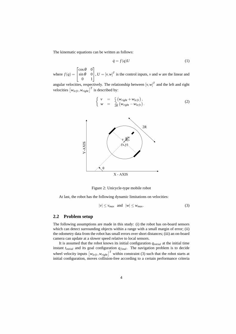
The kinematic equations can be written as follows:

q = f (q)U (1)

where f (q) =

cosθ 0sinθ 0

0 1

, U = [v,w]T is the control inputs,v andw are the linear and

angular velocities, respectively. The relationship between[v,w]T and the left and rightvelocities

[wle f t,wright

]Tis described by:

{v = r

2

(wright +wle f t

),

w = r2R

(wright −wle f t

).

(2)

��

�

�

�

� �

�������

����

�

����

���������

���

Figure 2: Unicycle-type mobile robot

At last, the robot has the following dynamic limitations on velocities:

|v| ≤ vmax and |w| ≤ wmax. (3)

2.2 Problem setup

The following assumptions are made in this study: (i) the robot has on-board sensorswhich can detect surrounding objects within a range with a small margin of error; (ii)the odometry data from the robot has small errors over short distances; (iii) an on-boardcamera can update at a slower speed relative to local sensors.

It is assumed that the robot knows its initial configurationqinitial at the initial timeinstanttinitial and its goal configurationqf inal . The navigation problem is to decide

wheel velocity inputs[wle f t,wright

]Twithin constraint (3) such that the robot starts at

initial configuration, moves collision-free according to a certain performance criteria

4

and arrives in a neighbourhood of the final configuration. To solve this problem, onecan make the following choices without loss of any generality1:

• The robot’s geometric shape is represented by a 2-D circle of centreC = (x,y)and of radiusR. Its motion is controlled but nonholonomic and is representedby the velocity vectorU(t). The range of its sensors is also described by a circlecentrered atC and of radiusRs.

• The itextth object,i = 1, . . . ,No, will be represented by a circle centrered at pointOi = (Xi ,Yi) and of radiusr i , denoted byBi(Oi , r i).

3 Motion planning

Depending on the distance that the robot has to travel, the computation of a completetrajectory from start until finish may be computationally too expensive. Moreover, theenvironment is partially known and further explored in real time. Therefore, the tra-jectory has to be computed gradually over time while the mission unfolds. It can beaccomplished using an on-line receding horizon planner [15], in which partial trajec-tories from an initial state toward the goal are computed by solving an optimal controlproblem over a limited horizon.

3.1 Receding horizon planner

Contrary to most of the existing trajectory generation modules, the proposed motionplanner explicitly takes into account the real time constraint. Indeed, the mobile robothas a limited time to compute its reference optimal trajectoryqre f (t). The timeδ t al-located to make its decision depends on its perception sensors, its computation delays,etc. The proposed algorithm relaxes the constraint that the final point is reached inthe planning horizon. In each receding horizon planning problem, the same planninghorizonTp ∈ R+ and update periodTc ∈ R+ (δ t ≤ Tc < Tp) are used. At each update,denotedτk (k∈ N),

τk = tinitial +kTc, (4)

the robot computes an optimal collision-free trajectory satisfying constraints (1) and(3) using only local information.

To distinguish the different trajectories, we introduce the following notations:

q(t,τk) : the predicted trajectory over any interval[τk,τk +Tp] ,qre f (t,τk) : the optimal planned trajectory over any interval[τk,τk+1τk +Tc[ ,q(t) : the actual trajectory.

The associated control inputs areU(t,τk), Ure f (t,τk) andU(t).

1It is trivial to allow the envelope of either the robot or an obstacle to be represented by union/intersectionof several circles. The envelopes could also be polygonal. Mathematically, circular envelopes can be repre-sented by second order inequalities while polygonal envelopes can be described by first order linear inequal-ities.

5

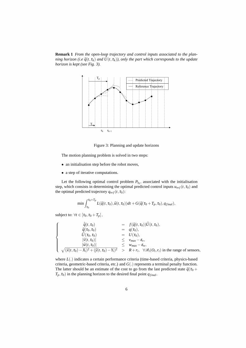
Remark 1 From the open-loop trajectory and control inputs associated to the plan-ning horizon (i.eq(t,τk) andU(t,τk)), only the part which corresponds to the updatehorizon is kept (see Fig. 3).

�

�������������������������� �

��

��

��� �����

�������������������������� �

Figure 3: Planning and update horizons

The motion planning problem is solved in two steps:

• an initialisation step before the robot moves,

• a step of iterative computations.

Let the following optimal control problemPτ0, associated with the initialisationstep, which consists in determining the optimal predicted control inputsure f (t,τ0) andthe optimal predicted trajectoryqre f (t,τ0):

min∫ τ0+Tp

τ0

L(q(t,τ0), u(t,τ0))dt+G(q(τ0 +Tp,τ0),qf inal),

subject to:∀t ∈ [τ0,τ0 +Tp] ,

˙q(t,τ0) = f (q(t,τ0))U(t,τ0),q(τ0,τ0) = q(τ0),U(τ0,τ0) = U(τ0),|v(t,τ0)| ≤ vmax− εv,|w(t,τ0)| ≤ wmax− εw,√

(x(t,τ0)−Xi)2 +(y(t,τ0)−Yi)2 > R+ r i , ∀Bi(Oi , r i) in the range of sensors,

whereL(.) indicates a certain performance criteria (time-based criteria, physics-basedcriteria, geometric-based criteria, etc.) andG(.) represents a terminal penalty function.The latter should be an estimate of the cost to go from the last predicted stateq(τ0 +Tp,τ0) in the planning horizon to the desired final pointqf inal .

6

Remark 2 The inclusion of constantsεv ∈ R+ andεw ∈ R+ in the constraints of themotion planning problem guarantees that there is sufficient control authority to trackthe optimal planned trajectory (see Section 4).

This process is then repeated during the robot’s movement, over the interval[τ0,τ1],and so on until its reaches a neighbourhood of the goalqf inal . As such, new detectedobstacles can be taken into account in the next iteration. Over any interval[τk,τk+1](k∈N), the following optimal control problemPτk+1, associated with the(k+1)th step,which consists in determining the optimal predicted control inputsure f (t,τk+1) and theoptimal predicted trajectoryqre f (t,τk+1) is solved:

min∫ τk+1+Tp

τk+1

L(q(t,τk+1), u(t,τk+1))dt+G(q(τk+1 +Tp,τk+1),qf inal), (5)

subject to:∀t ∈ [τk+1,τk+1 +Tp] ,

˙q(t,τk+1) = f (q(t,τk+1))U(t,τk+1), (6)

q(τk+1,τk+1) = q(τk+1,τk), (7)

U(τk+1,τk+1) = U(τk+1,τk), (8)

|v(t,τk+1)| ≤ vmax− εv, (9)

|w(t,τk+1)| ≤ wmax− εw, (10)√(x(t,τk+1)−Xi)2 +(y(t,τk+1)−Yi)2 > R+ r i ,

∀Bi(Oi , r i) in the range of sensors. (11)

OncePτk+1 is solved, the optimal reference trajectory and control inputs over the in-terval [τk+1,τk+2] , are stored for use at the next module (i.e. trajectory tracking con-troller).

Remark 3 One can note that constraints (7) and (8) on the initial conditions needthe optimal predicted control inputsU(τk+1,τk) and trajectoryq(τk+1,τk) computed inthe previous step. Therefore, in the proposed strategy, the receding horizon planner isnot used in order to reject external disturbances or inherent discrepancies between themodel and the real process, as it is usually done [16]. However, it takes into accountthe computation timeδ t. Fig. 4 gives an overview of the receding horizon planner.

Remark 4 A compromise must be done between reactivity and optimality. Indeed, theplanning horizonTp must be sufficiently small in order to have good enough results interm of optimality for trajectory planning. However, it must be higher than the updatehorizonTc in order to guarantee the reactivity and obstacle avoidance for next recedinghorizon planning problems.

3.2 Technique for solving receding horizon planning problems

There are three components to the real time resolution of the optimal control problemsPτk (k∈N): determination of the flat outputs, B-spline parametrization and constrainedfeasible sequential quadratic programming.

7

�

����������������������� �

���������������������� ������

�������

���

�������������

������������������������

��������

��������������

�

��������

����������������

�

�����

Figure 4: Implementation of the receding horizon planner

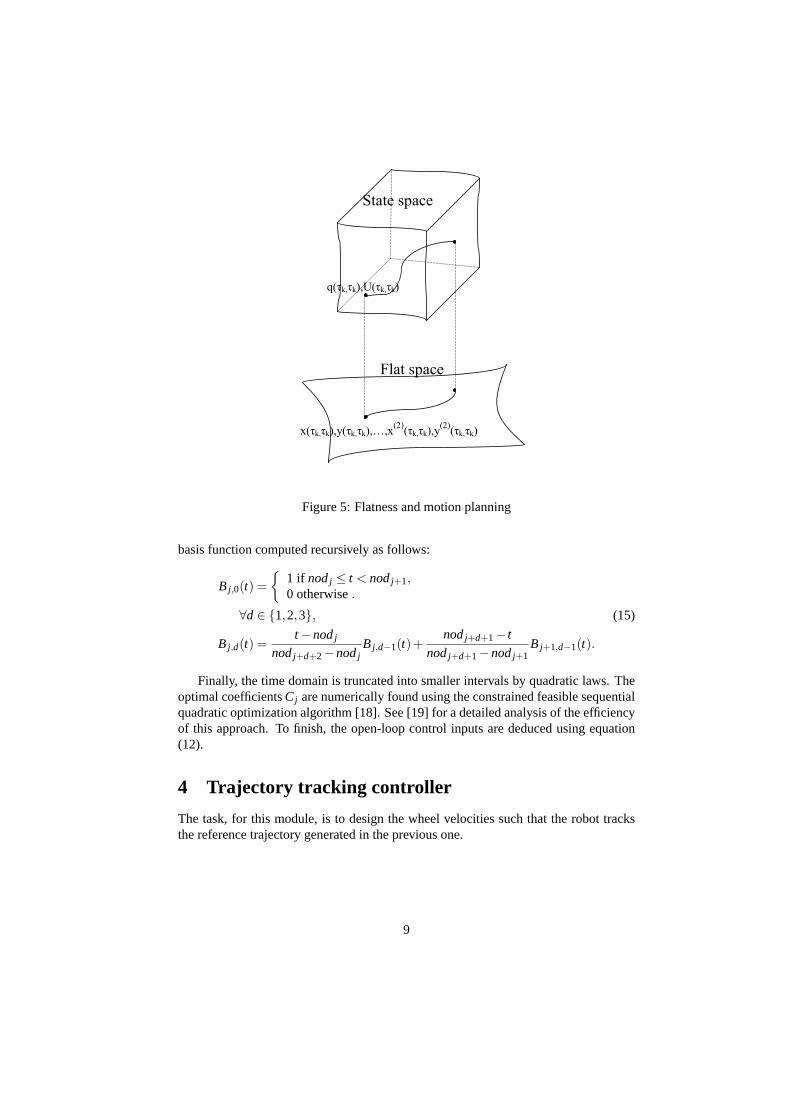
The key approach is to determine outputs such that equation (1) is mapped to alower dimensional output space. It will imply that the problem becomes computionallymore efficient to solve. Using the flatness property of system (1) (see [17] for furtherdetails about flatness), all system variables can be differentially parameterized byx, yand a finite number of their time derivatives. Indeed,θ , v andw can be expressed byx,y and their first and second time derivatives, i.e.

θ = arctanyx, v =

√x2 + y2 and w =

yx− xyx2 + y2 . (12)

Once the performance criteria (5) and constraints (6)-(11) are mapped into the flatoutput space, the optimal predicted trajectory is planned in this space (see Fig. 5).

Then, in order to transform the optimal trajectory generation problem into a pa-rameter optimization one, a piecewise polynomial function, B-spline, is adopted toapproximate the trajectory. The B-spline functions are chosen as basis functions dueto their flexibility and ease of enforcing continuity across breakpoints. B-Spline is thefunction defined by a series of knots called control knots. In our study, the three-orderB-spline basis functions are used to parameterize the trajectory. For problemPτk, thetime interval[τk,τk +Tp] is divided intonknot equal segments withnknot+4 knots to becontrol knots:

nod0 = . . . = nod3 = τk < nod4 < .. . < nodnknot+3 = τk +Tp (13)

The trajectories of the flat outputs are written in terms of finite dimensional B-splinecurves as: [

x(t,τk)y(t,τk)

]=

3+nknot

∑j=1

CjB j,3(t) (14)

whereCj ∈ R2 are the coefficients of the third-order B-spline andB j,3 is the B-spline

8

�

������������

���������

�� �� ����� �� ���

�� �� ����� �� ���������� �� ����

���� �� ���

Figure 5: Flatness and motion planning

basis function computed recursively as follows:

B j,0(t) ={

1 if nodj ≤ t < nodj+1,0 otherwise.

∀d ∈ {1,2,3}, (15)

B j,d(t) =t−nodj

nodj+d+2−nodjB j,d−1(t)+

nodj+d+1− t

nodj+d+1−nodj+1B j+1,d−1(t).

Finally, the time domain is truncated into smaller intervals by quadratic laws. Theoptimal coefficientsCj are numerically found using the constrained feasible sequentialquadratic optimization algorithm [18]. See [19] for a detailed analysis of the efficiencyof this approach. To finish, the open-loop control inputs are deduced using equation(12).

4 Trajectory tracking controller

The task, for this module, is to design the wheel velocities such that the robot tracksthe reference trajectory generated in the previous one.

9

4.1 Formulation of the tracking problem

The reference trajectory(xr ,yr ,θr), generated by the motion planning algorithm fulfillsthe differential equation:

xr

yr

θr

=

cosθr 0sinθr 0

0 1

[vr

wr

], (16)

where the desired velocitiesvr andwr satisfy:

|vr | ≤ vmax− εv and |wr | ≤ wmax− εw.

By directly applyingvr andwr , the robot does not follow the reference trajectory witha good accuracy. It is obvious that the real control inputsv andw rely on the statemeasurementsx, y andθ . Due to measurement noise and modeling uncertainties, thereare input uncertainties forv andw. That is to say, the actual equation of the robottrajectory fulfills the following uncertain differential equation:

xyθ

=

cosθ 0sinθ 0

0 1

[v+δv

w+δw

](17)

whereδv andδw represent the uncertainties.Control inputsv andw must be designed such that system (17) follows reference

(16) in spite of the perturbations. In fact, the goal is to asymptotically stabilize thetracking errorsex = xr − x, ey = yr − y andeθ = θr − θ to zero while respecting thesaturation constraints (3).

Transforming the tracking errors expressed in the inertial frame to the robot frame,the error coordinates can be denoted as:

e1

e2

e3

=

cosθ sinθ 0−sinθ cosθ 0

0 0 1

ex

ey

eθ

.

Accordingly, the tracking error dynamics is represented by:

e= f1(e, t)+ f2(e, t)(U +δ ) (18)

where

e = [e1,e2,e3]T ,U = [v,w]T ,δ = [δv,δw]T ,

f1(e, t) =

vr cose3

vr sine3

wr

,

f2(e, t) =

−1 e2

0 −e1

0 −1

.

10

It should be pointed out that such a system cannot be stabilized by continuouslydifferentiable, time-invariant, state feedback control laws. In this paper, we combineintegral sliding mode control with time-varying state feedback in order to further ro-bustify against perturbations.

4.2 Proposed methodology

The basic idea is to use an integral sliding mode controller to reject the matched pertur-bation (i.e. perturbations that enter the state equation at the same point as the controlinputs). The integral sliding mode control algorithm is designed in two steps [20]:

1. the selection of a suitable integral sliding variables such that, while sliding, thecontrol objective is fulfilled,

2. the design of corresponding control inputsU constraining the system trajectoriesto evolve on the sliding surface from the initial time instant.

For system (18), the control law is defined as follows:

U(q, t) = U0(q, t)+U1(q, t). (19)

The nominal controlU0(q, t) is responsible for the performance of the nominal system.U1(q, t) is a discontinuous control action that reject the perturbations by ensuring thesliding motion.

4.2.1 Integral sliding mode controller

Let us define the sliding variables(q, t) = [s1(q, t),s2(q, t)]T ∈ R2 as:

s(q, t) = P

[e(t)−e(tinitial )−

∫ t

tinitial

( f1(e,ν)+ f2(e,ν)U0(q,ν))dν], (20)

where matrixP ∈ R2×3 is such thatP f2(e, t) is invertible for all t ∈ R+. Making

P =[−1 0 0

0 0 −1

], the above condition is fulfilled. One can note that, at the initial

time instantt = tinitial , the sliding variable satisfiess(q, t) = 0, such that the controlledsystem always starts on the sliding surface{s(q, t) = 0}.

Remark 5 To simplify notation, we will omit some of the functions’ arguments fromnow on.

Based on the following Lyapunov function candidate,V = 12sTs, the discontinuous

control term can be determined such thatV < 0, guaranteeing the attractivity of the

11

sliding surface. One can obtain:

V = sT (Pe−P( f1 + f2U0))

= sT (P( f1 + f2(U +δ ))−P( f1 + f2U0))

= sT (P f2(U1 +δ ))

=([P f2]

T s)T

(U1 +δ )

=[s1 −e2s1 +s2

](U1 +δ ) < 0

The above condition holds if:

U1 =[ −M1sign(s1)−M2sign(−e2s1 +s2)

](21)

whereM1 andM2 are gain high enough to enforce the sliding motion.

The trajectory evolves on{s= 0} from t = tinitial and remains there in spite of theperturbations. To determine the motion equations on the sliding surface, the equivalentcontrol method [21] is used. The time derivative of the sliding variable is:

s = P(e− f1− f2U0)= P f2(U1 +δ )

The equivalent control is obtained by solving the equations= 0 for U1:

U1eq =−δ (22)

By substitutingU1eq for U1 in (18), one can obtain the sliding dynamics:

e= f1(e)+ f2(e)U0 (23)

Remark 6 From equation (23), several conclusions can be drawn. Firstly, the slidingdynamics do not contain the matched perturbation: it has been successfully rejected.Secondly, with respect to the conventional sliding mode control, we have gained someextra degrees of freedom. Indeed,U0 can be used in order to stabilize the nominalsystem and to deal with the unmatched perturbation.

4.2.2 Time-varying state feedback controller

The second part of the controller design is to find a saturated control lawU0 such thatthe sliding dynamics (23) is globally asymptotically stable. The chosen control lawU0 has been developed by Jiang in [22]. The motivation for such a choice is that thisdesign takes into account the actuator bounds. It is described by:

U0 =

[v0 = vr cose3 +λ3 tanhe1

w0 = wr + λ1vr e21+e2

1+e22

sine3e3

+λ2 tanhe3

](24)

12

Note that the positive parametersλ1, λ2 andλ3 can be designed such that the boundsof the controls are met for our controllers. Indeed, it can be seen that:

|v0| ≤ vmax− εv +λ3, |w0| ≤ wmax− εw +λ1(vmax− εv)

2+λ2

Remark 7 The control gains can be designed such that the bounds on the control in-puts are satisfied. In order to design these constants, a compromise must be foundbetween the optimality, the performance and the robustness with respect to perturba-tions.

From (2), it is straightforward to obtain the wheel velocities:{

wright = v−Rwr

wle f t = v+Rwr

5 Experimental results

5.1 Experimental setup

The proposed motion planning and control algorithms are implemented on the mobilerobot Pekee manufactured at Wany Robotics company (see Fig. 6). An overview ofthe experimental setup is shown in Fig. 7. An Intel486 micro-processor runningat 75MHz hosts the integral sliding mode controller written in C. The robot operatesunder linux real time and its software integrates sensor and communication data. Itcommunicates through wireless Ethernet capable of transmitting data up to3Mb/s.One miniature color vision camera C-Cam8 is mounted on the robot. A C programaccesses the streaming data coming into the frame grabber from the camera and storesthe data in a320×240image file. The robot is also equipped with 15 infra-red sensorsused for local identification of the environment and two encoders.

�

Figure 6: Pekee mobile robot

13

�

������������� ����������

• �������������

• ������� �������

�

�

�

�

�

�

�

�

��������������������

� ���������������

�

�

• ����� !��������

• ������������"�����

"�� ��������

�

�

�

�

�

�

�

#��$��"�����������%&�'(����

� ���������������

�

• ��)�����"�"����

• *�����"����

+�)���� ��

������

���,� ��-�

• ��)�����"�"����

• *�����"����

+�)���� ��

������

���,� ��-�

Figure 7: Overview of the experimental setup

The vehicle’s wheelbase is taken toR= 0.3m with vmax= 0.8m/s, wmax= 5rad/sand the sampling period is100ms. The computation timeδ t including the imageprocessing and the motion planning algorithm is about two minutes on the on-board75MHz PC. In order to decrease the computation delay, we used the socket protocolcommunication and wireless communication link. The vision data are sent to a PentiumIV 2.4GHzPC for image processing and for the generation of the optimal trajectory.This protocol enables to reduceδ t to less than0.2s.

5.2 Experimental results

We run experiments on different environments cluttered with obstacles. The corre-sponding videos are available at: http://www.isen.fr/∼sst lille/fichiers/Icra.wmv.

In these experiments, obstructed areas are created with circular obstacles in theworkspace. Some of them are initially out of view from the robots’ on-board sensorsand may be discovered during the robot movement. The performance criteria is thelength of the traveled distance. For the motion planner, the chosen parameters aredescribed in Tab. 1. Furthermore, the parameters for the tracking algorithm are givenin Tab. 2. For comparison purpose, the gainsM1 andM2 needed to enforce the slidingmode are the same in all the experiments in which they occur. The discontinuous

14

Tp 2sTc 0.5s

nknot 6εv 0.3m/sεw 1rad/s

Table 1: Parameters of the motion planner

λ1 0.5λ2 1λ3 0.5M1 0.2M2 0.2

Table 2: Parameters of the tracking algorithm

controls are approximated by:

U1 =

[−M1

s1|s1|+0.0001

−M2−e2s1+s2

|−e2s1+s2|+0.0001

]

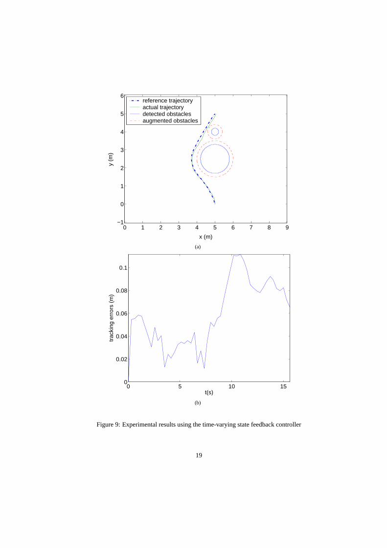
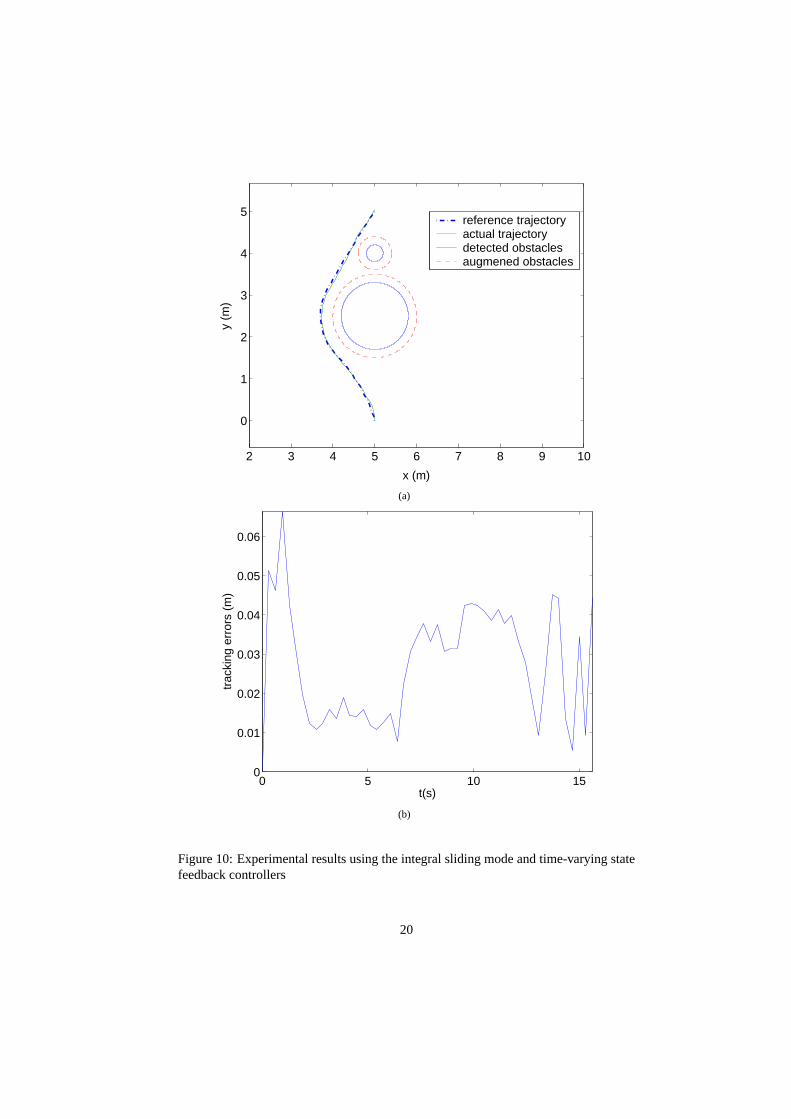
Figures 10(a) and 11 depict the executed trajectories in unknown environments.First, the robot visualizes the scene and applies the image processing. The nearest ob-stacles in view from its on-board sensors are detected. In order to take into accountthe size of the robot, the radius of these obstacles is increased by0.3m (dotted linesaround obstacles). According to the detected obstacles, a collision-free trajectory isplanned. Then, the integral sliding mode controller enables to track the desired trajec-tory in spite of uncertainties and errors. During the execution, the robot plans, in realtime, its next optimal collision-free trajectory by taking into account new informationfrom its infra-red and camera sensors. The effectiveness, perfect performance of ob-stacle avoidance, real time and high robustness properties are demonstrated by theseexperimental results.

Figures 8, 9 and 10 highlight the performance for the proposed tracking module.The first experiment is made without using feedback controller. By directly apply-ing the open-loop control inputs, the robot does not follow its planned trajectory dueto measurement noise and modeling uncertainties. One can see in Fig. 8(b) that thedistance between the actual and planned trajectories, i.e.

√(x−xr)2 +(y−yr)2, di-

verges. The second one is made using only the time-varying state feedback controller.The third experiment is made using the combination “integral sliding mode controllerplus the time-varying state feedback controller”. One can note that using only the time-varying state feedback controller, the robustness performance is not good enough. Theuse of an integral sliding mode controller enables to improve the precision motiontracking.

15

6 Conclusion

An architecture for real time navigation of an autonomous mobile robot evolving in anuncertain environment with obstacles is proposed. It provides the following practicaladvantages:

• First, it enables to take into account the dynamic limitations on velocities.

• Further, receding horizon planner is a viable method for real time trajectory gen-eration. Depending on computing resources, the use of flatness, B-spline para-metrization and constrained feasible sequential quadratic programming can takeless than one second to compute an optimal collision-free trajectory.

• Also, the combination of integral sliding mode control with other methods liketime-varying state feedback improves the robustness properties of the closed-loop system. Therefore, high precision trajectory tracking is achieved in spite ofuncertainties and modeling errors.

Experimental results show the effectiveness of our practical scheme (real time, highrobustness properties and good performance for obstacle avoidance).

References

[1] J.-P. Laumond, “Robot Motion planning and Control”, Springer-Verlag, 1998.

[2] J. C. Latombe, “Robot Motion Planning”, Boston: Kluwer Academic Publisher,1991.

[3] M. Salichs and L. Moreno, “Navigation of mobile robots: open questions”,Ro-botica, 18, pp.227-234, 2000.

[4] Y. Chen and A. Desrochers, “Structure of Minimum-Time Control Law for Ro-botic Manipulators with Constrained Paths”,IEEE International Conference onRobotics and Automation, pp. 971-976, 1989.

[5] I. Kolmanovsky and N. H. McClamroch, “Developments in nonholonomic con-trol problems”,IEEE Control Systems Magazine, 15, pp. 20-36, 1995.

[6] R. Brockett, “Asymptotic stability and feedback stabilization”, in R. Brockett, R.Millman, and H. Sussmann (eds.), Differential geometric control theory (Boston,MA: Birkhauser), pp. 181-195, 1983.

[7] J. Pomet, “Explicit design of time-varying stabilizing control laws for a class ofcontrollable systems without drift”,Systems and Control Letters, 18(2), pp. 147-158, 1992.

[8] C. Samson, “Control of chained systems: Application to path following and time-varying point-stabilization of mobile robots”,IEEE Trans. on Automatic Control,40, pp. 64-77, 1995.

16

[9] R. Murray and S. Sastry, “Nonholonomic Motion Planning: Steering Using Sinu-soids”,IEEE Trans. on Automatic Control, 38(5), pp. 700-716, 1993.

[10] J. P. Hespanha and A. S. Morse, “Stabilization of nonholonomic integrators vialogic-based switching”,Automatica, 35(3), pp 385-393, 1999.

[11] Z. P. Jiang and H. Nijmeijer, “Tracking control of mobile robots: a case study inbacksteeping”,Automatica, 33(7), pp. 1393-1399, 1997.

[12] T. Floquet, J. P. Barbot and W. Perruquetti, “Higher-order sliding mode stabi-lization for a class of nonholonomic perturbed systems”,Automatica, 39(6), pp.1077-1083, 2003.

[13] S. Monaco and D. Normand-Cyrot, “An introduction to motion planning undermultirate digital control”,Proceedings of the31st Conference on Decision andControl, pp. 1780-1785, 1992.

[14] C. de Wit and O. Sordalen, “Exponential stabilization of mobile robots with non-holonomic constraints”,IEEE Trans. on Automatic Control, 37(11), pp. 1791-1797, 1992.

[15] D. Mayne, J. Rawlings, C. Rao and P. Scokaert, “Constrained model predicitivecontrol: Stability and Optimality”,Automatica, 36, No 6, pp. 789-814, 2000.

[16] F. A. Cuzzolaa, J. C. Geromel and M. Morari, “An improved approach for con-strained robust model predictive control”,Automatica, 38, No 7, pp. 1183-1189,2002.

[17] M. Fliess, J. Levine, Ph. Martin and P. Rouchon, “Flatness and defect of nonlinearsystems: introductory theory and examples”,Int. J. of Control, 61(6), pp 1327-1361, 1995.

[18] C. Lawrance, J. Zhou and A. Tits, “User’s guide for CFSQP Version 2.5”,Institutefor Systems Research, University of Maryland, College Park.

[19] M. B. Milam, “Real time optimal trajectory generation for constrained dynamicalsystems”,California Institute of Technology, Dissertation, 2003.

[20] V. Utkin and J. Shi, “Integral sliding mode in systems operating under uncertaintyconditions”,Proceedings of the35th Conference on Decision and Control, pp.4591-4596, 1996.

[21] V. Utkin, “Sliding Modes Control in Electromechanical Systems”, Taylor andFrancis, 1999.

[22] Z. P. Jiang, E. Lefeber and H. Nijmeijer, “Saturated stabilization and track controlof a nonholonomic mobile robot”,Syst. and Cont. Letters, 42(5), pp. 327-332,2001.

17

2 3 4 5 6 7 8 9

0

0.5

1

1.5

2

2.5

3

3.5

4

4.5

5

x (m)

y (m

)

reference trajectoryactual trajectorydetected obstaclesaugmented obstacles

(a)

0 5 10 150

0.1

0.2

0.3

0.4

0.5

0.6

0.7

0.8

0.9

1

t (s)

trac

king

err

ors

(m)

(b)

Figure 8: Experimental results without using the trajectory tracking module

18

0 1 2 3 4 5 6 7 8 9−1

0

1

2

3

4

5

6

x (m)

y (m

)

reference trajectoryactual trajectorydetected obstaclesaugmented obstacles

(a)

0 5 10 150

0.02

0.04

0.06

0.08

0.1

t(s)

trac

king

err

ors

(m)

(b)

Figure 9: Experimental results using the time-varying state feedback controller

19

2 3 4 5 6 7 8 9 10

0

1

2

3

4

5

x (m)

y (m

)reference trajectoryactual trajectorydetected obstaclesaugmened obstacles

(a)

0 5 10 150

0.01

0.02

0.03

0.04

0.05

0.06

t(s)

trac

king

err

ors

(m)

(b)

Figure 10: Experimental results using the integral sliding mode and time-varying statefeedback controllers

20

−2 −1 0 1 2 3 4 5 60

1

2

3

4

x (m)

y (m

)

actual trajectorydetected obstaclesaugmented obstacles

Figure 11: Experimental results using the integral sliding mode and time-varying statefeedback controllers in a more complex map

21