Embed Size (px)
Citation preview

ST. ANTHONY FALLS LABORATORY Engineering, Environmental and Geophysical Fluid Dynamics
PROJECT REPORT NO. 494
Performance Assessment of Underground Stormwater Treatment Devices
By
Matthew A. Wilson, John S. Gulliver, Omid Mohseni, and Ray M. Hozalski
Prepared for Local Road Research Board
and Twin Cities Metropolitan Council
July 2007 Minneapolis, Minnesota

i
The University of Minnesota is committed to the policy that all persons shall have equal access to its programs, facilities, and employment without regard to race, religion, color, sex, national origin, handicap, age or veteran status.

ii

iii
Abstract Proprietary underground devices are often used for stormwater treatment in urban areas due to tight space constraints. Most of these devices are designed to remove suspended solids from stormwater runoff prior to discharge into lakes, rivers, and streams via the physical separation process of sedimentation. Data on the performance of installed devices are limited and existing data are questionable because of the problems associated with assessment via monitoring. The objectives of this research were to: (1) investigate the feasibility and practicality of field testing for assessing the performance of underground devices, (2) evaluate the effects of sediment size and stormwater flow rate on the performance of four devices from different manufacturers, and (3) develop a universal approach for predicting the performance of a device for any given application. For the field testing, a controlled and reproducible synthetic storm event containing sediment of a fixed size distribution and concentration is fed to a pre-cleaned device. The captured sediment is then removed, dried, sieved, and weighed. Universal performance models were developed from the results of this work and parallel laboratory testing of two other full-scale devices using the Peclet number, which explains two major processes in performance: (1) advection or settling of particles and (2) turbulent diffusion or resuspension of particles. The universal performance models will improve the selection and sizing of these devices and their overall performance after installation.

iv

v
Acknowledgements We would like to thank the Local Road Research Board (LRRB) and the Metropolitan Council for providing funding for this project. Jon Haukaas and Sue McDermott Alan Rindels were the technical liaison and the administrative liaison, respectively, on behalf of the LRRB, and Jack Frost was the project officer from the Metropolitan Council.
In addition, Dave Olson and the City of New Brighton, Scott Anderson and the City of Saint Louis Park, Ryan Bluhm of Master Engineering, Jon Haukaas and the City of Fridley, and Rich Profaizer and Jeff Grant and the City of Minneapolis are all owed a debt of gratitude for donating the use of City vacuum trucks and maintenance crew time for the clean out of the stormwater manholes prior to the commencement of field testing. Jon Haukaas and the City of Fridley Fire Department provided further assistance with their donation of 300 feet of fire hose and hydrant fittings for project use.
Andrew Sander, Joshua Brand, Adam Markos, Geoffrey Fischer, and Andrew Fyten assisted with fieldwork and laboratory analysis, and Ben Erickson produced an instructional video on field testing.
Project Technical Advisory Panel members were Jon Haukaas (City of Fridley), Jack Frost (Metropolitan Council), Alan Rindels (MnDOT), Marilyn Jordahl-Larson (MnDOT), Scott Carlstrom (MnDOT), Sue McDermott (City of Mendota Heights), and Judy Sventek (Metropolitan Council). Finally, the cooperation by proprietary device manufacturers Environment21, CONTECH, and Imbrium Systems, Inc has been appreciated.

vi

vii
Table of Contents
Abstract .................................................................................................................................... iii
Acknowledgements................................................................................................................... v
List of Tables ........................................................................................................................... ix
List of Figures .......................................................................................................................... xi
1. Introduction........................................................................................................................... 1
1.1. Previous Studies ....................................................................................................... 1 1.2. Heavy Metals and Particulate Phosphorus Association to Sediment Particles ........ 2
2. Methods and Materials.......................................................................................................... 7
2.1. Site Selection............................................................................................................ 7 2.2. Suspended Solids...................................................................................................... 7 2.3. Field Testing............................................................................................................. 7
3. Scaling and Removal Efficiency........................................................................................... 9
4. Results................................................................................................................................. 11
5. Discussion ........................................................................................................................... 19
6. Application of Results......................................................................................................... 21
7. Conclusions and Recommendations ................................................................................... 23
8. References........................................................................................................................... 25
Appendix A: Sieving Operation.............................................................................................. 29
Appendix B: Device Function Description............................................................................. 37
B.1. Environment21 V2B1 Model 4 ............................................................................. 39 B.2. Vortechs Model 2000 ............................................................................................ 40 B.3.Stormceptor STC4800 ............................................................................................ 43 B.4. CDS Model PMSU20_15 ...................................................................................... 45
Appendix C: Site Description, Preparation, and Field Test Procedure................................... 49
C.1.Test Site Description and Preparation .................................................................... 51 C.2.V2B1 Model 4 ........................................................................................................ 51 C.3. Vortechs Model 2000 ............................................................................................ 58 C.4.Stormceptor STC4800 ............................................................................................ 65 C.5. CDS PMSU20_15.................................................................................................. 70 C.6. Field Test Procedure.............................................................................................. 75
Appendix D: Field Testing Equipment Checklist................................................................... 77

viii

ix
List of Tables Table 1.1: Comparison of the known concentration of suspended sand and silt in a water
column with the measured concentration in samples obtained by autosampling equipment, with a 9.5 mm sampling tube placed near the pipe invert.............................. 2
Table 1.2: Association of metals to particular sediment size ranges ....................................... 4
Table A.1: Sample initial results of field testing showing overlapping behavior .................. 33
Table A.2: Results of sieving analysis indicating scattering behavior around ‘correct’ size. 34

x
xi
List of Figures Figure 1.1: Sorption isotherms for heavy metals to sandy lake sediments (Echeverria, 1998).
........................................................................................................................................... 5
Figure 1.2: Sorption isotherms for phosphorus to lake sediments, sorted by sediment size (from Wang, 2006)............................................................................................................ 6
Figure 4.1: Removal efficiency versus Pe for the new BaySaver Model 1k in rectangular coordinates (after Carlson et al., 2006) ........................................................................... 13
Figure 4.2: Removal efficiency versus Pe for the BaySaver Model 1k (after Carlson et al., 2006). .............................................................................................................................. 13
Figure 4.3: Removal efficiency of the Model 3 ecoStorm versus Pe (from Mohseni and Fyten, 2007). ................................................................................................................... 14
Figure 4.4: Removal efficiency versus Pe for the V2B1 Model 4, reflecting removal by 1) solely the settling chamber, and 2) total removal by the combination of the settling chamber and floatables trap. ........................................................................................... 15
Figure 4.5: Removal efficiency versus Pe for the Vortechs Model 2000, reflecting removal by 1) solely the settling chamber, and 2) total removal by the combination of the settling chamber and floatables trap. ........................................................................................... 16
Figure 4.6: Removal efficiency versus Pe for the Stormceptor STC4800............................. 16
Figure 4.7: Removal efficiency versus Pe for the CDS PMSU20_15, reflecting removal by 1) solely the settling chamber, and 2) total removal by the combination of the settling chamber and floatables trap. ........................................................................................... 17
Figure 6.1: Particle size distribution in stormwater runoff from an urban freeway watershed, along with the range of gradations measured in six runoff events (Li et al., 2005)........ 22
Figure A.1: Four Ro-Tap sieve shakers were relocated to the Quonset hut adjacent to SAFL to maximize operator productivity.................................................................................. 31
Figure A.2: Use of a rectangular sieve shaker table and customized screens increased productivity significantly over commonly used Ro-Tap shakers. .................................. 35
Figure B.1: Plan and section of V2B1 Model 4, dual manhole stormwater treatment device installed at Rice Creek Road & Long Lake Road, New Brighton, MN (Environment21, 2005) ............................................................................................................................... 40
Figure B.2: Site drainage layout for installation of Vortechs Model 2000............................ 41
Figure B.3: General plan and section of a Vortechs Model 2000 stormwater treatment device (CONTECH Stormwater Solutions: Vortechs 2007)...................................................... 43
Figure B.4: General plan and section of a Stormceptor STC 4800 stormwater treatment device. In the section view of the depth to storm drain inlet, and the height of the treatment sump, the drawing indicates a varying depth and a minimum depth, respectively. (Stormceptor, 2007)................................................................................... 45
xii
Figure B.5: Plan and section views of the CDS device evaluated at West Franklin & Ewing Avenue South in Minneapolis, MN (CDS Technologies, Inc., 2006). ........................... 47
Figure C.1: Plan and profile of Environment21 V2B1 Model 4 installation site in New Brighton, MN.................................................................................................................. 52
Figure C.2: Pre-calibrated 0.38 m (15 in) circular weir installed downstream of the V2B1. Pressure transducer and transducer anchoring not shown. This weir location provided free outfall conditions at all flowrates due to the PVC pipe’s favorable elevation vs. the existing 0.9 m (36 in) storm drain pipe it discharged into. ............................................. 53
Figure C.3: Customized influent delivery system from the water source at the hydrant to the injection point at rear. ..................................................................................................... 54
Figure C.4: 0.45 m (18 in) diameter inflatable plug loaned by the City of New Brighton Public Works for use where indicated in Figure C.3. ..................................................... 56
Figure C.5: Illustration of particle settling phenomenon inside the swirl chamber’s influent delivery pipe. It is clear that a sandbar has formed which is believed to contribute to further settling by reducing the vertical settling distance in this pipe. ........................... 56
Figure C.6: Use of a plastic sheet weighed down with sandbags to smoothly turn water downstream toward the V2B1 (water moving right to left) and therefore eliminate coarse sand particle settling in front of the inflatable plug due to weak vortices. .......... 57
Figure C.7: Contention of field testing with construction activities...................................... 57
Figure C.8: (Left) Water was initially able to flow between treatment manholes through an approximate 1.3 cm ( ½ in) gap between the PVC pipe and concrete manhole wall. (Right) The leaking gap was patched with Vulcum polyurethane to ensure proper system hydraulics. ....................................................................................................................... 58
Figure C.9: Site utility plan for installation of Vortechs Model 2000 in St. Louis Park, MN59
Figure C.10: Pre-calibrated 12” circular weir installed downstream of the Vortechs System. Pressure transducer and transducer anchoring not shown. This weir location provided free outfall conditions at all flow rates due to the favorable gradient across the manhole and downstream storm drain system............................................................................... 60
Figure C.11: Upstream portion of influent delivery system from the water source at the hydrant to the first reach of 4” fire hose in the foreground............................................. 60
Figure C12: Depiction of 4 inch fire hose used to span about 150 feet from the hydrant (not shown, see Figure C.11) to the influent injection point (right)....................................... 61
Figure C.13: 12” diameter inflatable plug loaned by the City of St. Louis Park Public Works for use at CBMH4 as shown in Figure C.12. .................................................................. 62
Figure C.14: Results of trial sediment feeding location 100 feet upstream of the Vortechs System. Sand settling in manhole in which it was fed (left) and along the 100-foot reach of the pipe leading to the Vortechs System (right). ........................................................ 63
Figure C.15: Sediment feeding location at STMH3B............................................................ 64
xiii
Figure C.16: View of the base of the stainless steel cylinder serving as a swirl chamber and new sealant applied (thicker section along lower right) to minimize improper hydraulics.......................................................................................................................................... 64
Figure C.17: Plan and profile for the Central Avenue 48-inch storm drain in which the Stormceptor was installed. .............................................................................................. 66
Figure C.18: Aerated 1.2 m (48 in) circular weir and pressure transducer cable as installed in the 1.2 m (48 in) RCP inside the manhole immediately downstream of the Stormceptor.......................................................................................................................................... 67
Figure C.19: Influent piping configuration, making use of the same hydrant fittings as at previous testing sites and a reach of fire hose to cover the ~10 m (35 ft) from hydrant to influent delivery point..................................................................................................... 68
Figure C.20: Illustration of sediment delivery system to prevent sediment deposition in the upstream pipe. In the photo at left, the sediment feeder augured into a 10.2 cm (2 in) diameter PVC pipe where it was met by wash water from a garden hose to prevent clogging at the elbow at the bottom of the pipe depicted at right................................... 69
Figure C.21: Downstream end of the sediment delivery piping system approximately 1.8 m (6 ft) upstream of the Stormceptor. A 90° elbow at the downstream end helped direct the flow to the centerline of the storm drain pipe for conveyance into the device. .............. 70
Figure C.22: Site layout and equipment for testing of CDS unit........................................... 71
Figure C.23: Initially installed weir and final weir directly behind it (upstream side), for flow rate measurement. The pressure transducer probe and clip anchoring upstream of the weir are not shown. ......................................................................................................... 72
Figure C.24: Influent piping system from hydrant to catch basin for CDS testing. .............. 73
Figure C.25: Sediment delivery system for CDS testing....................................................... 74
Figure C.26: Result of patchwork effort to repair a leaky seam between the stainless steel cylindrical screen and the fiberglass cylinder above it within the CDS. ........................ 74

xiv
1
1. Introduction
The 1987 Amendments to the Clean Water Act implemented a two-phase program to regulate stormwater discharge. Large municipalities, construction sites and industrial facilities were the focus of Phase I, while the scope was expanded in Phase II to include smaller municipalities, construction sites, and industrial facilities. As a result of this legislation, stormwater pollution prevention programs will be implemented on facilities owned and/or operated by the state, city, town, county, flood control, watershed district or other similar entities. In order to implement such programs, information is needed on the pollutant removal performance of stormwater best management practices (BMPs), such as detention ponds, bioretention systems, and proprietary underground devices.
Traditionally, stormwater BMPs have been evaluated via monitoring. Monitoring requires flow measurement and pollutant sampling at the inlet and outlet of the BMP in order to quantify pollutant removal performance. Monitoring offers the advantage of evaluating removal performance of a BMP when subject to the often wide variability in hydraulic and pollutant loads in the watershed of interest. Unfortunately, monitoring also has drawbacks related to pollutant sampling and transferability of the results to similar BMPs in other watersheds.
Proprietary underground devices are an attractive approach for removing leaves, trash, and suspended solids from stormwater runoff in dense urban areas due to their small footprint. These devices can function as stand-alone treatment systems or as a pre-treatment to other devices such as ponds and infiltration basins to reduce maintenance costs.
The goals of this assessment are to (1) investigate the practicality of controlled field testing as an alternative to field monitoring; (2) to evaluate the suspended solids removal capability of four proprietary underground structures when subjected to field testing with a wide range of sediment sizes and influent flow rates, and (3) develop a similarity approach for predicting the performance of a given device based on a dimensionless parameter (Peclet number). The main product of a field testing campaign is a performance function for each type of device in which removal efficiency is defined as a function of the Peclet number. This performance function can serve as a tool to predict the removal performance for a wide range of device sizes, influent flow rates, and particulate size characteristics. The performance function can also be used as a tool to accurately size a new stormwater treatment device, given a target removal efficiency, a runoff hydrograph for a particular recurrence interval, and a particle size distribution in the stormwater runoff.
1.1. Previous Studies A number of field monitoring studies have been undertaken to quantify the pollutant removal performance of underground stormwater treatment devices (Fassman, 2006; Roseen et al., 2005; ETV 2005a and 2005b; Bonestroo, Rosene, Anderlik and Associates, Inc. 2002 and 2003; Yu and Stopinksi, 2001; England, 2001; Strynchuk et al., 2000, and Waschbusch,
2
1999). These studies often differ in terms of experimental approach and evaluation criteria, making it difficult to compare the results. This comparison is further complicated by the fact that many types of proprietary structures exist, and that underground devices have been installed in a wide variety of watersheds, with diverse land uses, climate, and geology. Additionally, field monitoring relies on sampling, which is problematic for coarser materials like sand. As a result, obtaining a representative, unbiased sample at both the inlet and outlet of the treatment becomes a challenge (Andoh and Saul, 2003).
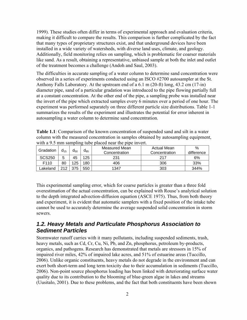
The difficulties in accurate sampling of a water column to determine sand concentration were observed in a series of experiments conducted using an ISCO #2700 autosampler at the St. Anthony Falls Laboratory. At the upstream end of a 6.1 m (20-ft) long, 43.2 cm (17-in) diameter pipe, sand of a particular gradation was introduced to the pipe flowing partially full at a constant concentration. At the other end of the pipe, a sampling probe was installed near the invert of the pipe which extracted samples every 6 minutes over a period of one hour. The experiment was performed separately on three different particle size distributions. Table 1-1 summarizes the results of the experiment and illustrates the potential for error inherent in autosampling a water column to determine sand concentration.
Table 1.1: Comparison of the known concentration of suspended sand and silt in a water column with the measured concentration in samples obtained by autosampling equipment, with a 9.5 mm sampling tube placed near the pipe invert. Gradation d15 d50 d85
Measured Mean Concentration
Actual Mean Concentration
% difference
SCS250 5 45 125 231 217 6% F110 80 125 180 406 306 33%
Lakeland 212 375 550 1347 303 344% This experimental sampling error, which for coarse particles is greater than a three fold overestimation of the actual concentration, can be explained with Rouse’s analytical solution to the depth integrated advection-diffusion equation (ASCE 1975). Thus, from both theory and experiment, it is evident that automatic samplers with a fixed position of the intake tube cannot be used to accurately determine the average suspended solid concentration in storm sewers.
1.2. Heavy Metals and Particulate Phosphorus Association to Sediment Particles Stormwater runoff carries with it many pollutants, including suspended sediments, trash, heavy metals, such as Cd, Cr, Cu, Ni, Pb, and Zn, phosphorus, petroleum by-products, organics, and pathogens. Research has demonstrated that metals are stressors in 15% of impaired river miles, 42% of impaired lake acres, and 51% of estuarine areas (Tuccillo, 2006). Unlike organic constituents, heavy metals do not degrade in the environment and can exert both short-term and long term toxicity due to their accumulation in sediments (Tuccillo, 2006). Non-point source phosphorus loading has been linked with deteriorating surface water quality due to its contribution to the blooming of blue-green algae in lakes and streams (Uusitalo, 2001). Due to these problems, and the fact that both constituents have been shown

3
to associate with particulates in stormwater runoff, both heavy metals and phosphorus are of special interest to this research. If a quantitative relationship can be definitively established between heavy metals and phosphorus association to particular sediment sizes, it is theorized that an annual removal of heavy metals and phosphorus by a sedimentation device can be estimated, given an understanding of how such a sedimentation device can be expected to remove sediment size fractions.
It is important to have accurate information on the particle size distribution in stormwater runoff when designing and sizing stormwater best management practices (BMPs). Many stormwater BMPs are designed to improve water quality through settling of pollutants. Settling can be effective for most sands in runoff, but clay and silt-sized particles may be discharged from BMPs due to their smaller settling velocities. Therefore, it is important to quantify the association of heavy metals and phosphorus to particular aggregate size fractions in order to estimate potential removal of metals and phosphorus by stormwater BMPs. In this way, the removal capability of a BMP for sediments in runoff can be a surrogate for the removal of heavy metals and phosphorus as well. In general, metal and phosphorus association increases with decreasing particle size (Sa, 2005; Bradl, 2004;; Johnson, 2003; Sutherland, 2003; Zhang, 2003; Zhu, 2003; Barbosa, 1999; and Philips, 1999), owing to smaller particles’ greater specific surface area in comparison to larger particles (Lau and Stenstrom, 2005), but there is a significant variability in metal concentrations.
There are factors that must be considered when drawing conclusions about metal concentration versus sediment size. Though attachment is often summarized with one magnitude, there are three retention processes at work contributing to metal association to sediment sizes: sorption, surface precipitation, and fixation (Bradl, 2004). Sorption of metals to sediment of diameter <63 µm has been shown to be pH dependent, with almost zero association at low pH, increasing to near complete sorption at intermediate pH, and decreasing again to near zero at high pH (Soltan, 2001). The presence of multiple metals in close proximity has been observed to interfere with and reduce the amount of each metal that is sorbed (Echeverria, 1998). However, there appears to be no competition between grain sizes in the sorption of a particular metal; that is, the total sorption by a particle size distribution is the sum of the sorption by each individual grain fraction (Huang and Wan, 1997). Association of metals also depends on the moisture condition of the soil, with significant differences for air-dry versus waterlogged soil, and of course on the concentration of metal present in the first place (Philips, 1999).
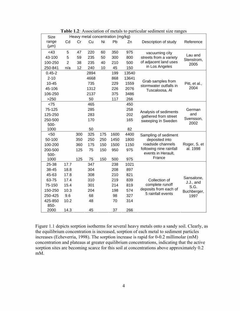
Table 1.2 summarizes the findings of several studies investigating how several heavy metals associate with particular sediment sizes. These results are highly dependent on the watershed in which the data were collected, which explains much of the variability in metal-sediment association.
4
Table 1.2: Association of metals to particular sediment size ranges Heavy metal concentration (mg/kg)
Cd Cr Cu Ni Pb Zn Description of study Reference Size
range (µm) <43 5 47 220 60 350 975
43-100 5 59 235 50 300 800 100-250 2 38 235 40 210 500 250-841 n/a 12 240 10 45 150
vacuuming city streets from a variety of adjacent land uses
in Los Angeles
Lau and Stenstrom,
2005
0.45-2 2894 199 13540 2-10 4668 868 13641 10-45 735 229 1559 45-106 1312 226 2076
106-250 2137 375 3486 >250 50 117 266
Grab samples from stormwater outfalls in
Tuscaloosa, Al
Pitt, et al., 2004
<75 465 450 75-125 285 258
125-250 283 202 250-500 170 165
500-1000 50 82
Analysis of sediments gathered from street sweeping in Sweden
German and
Svensson, 2002
<50 300 325 175 1600 4400 50-100 350 250 250 1450 1800
100-200 360 175 150 1500 1150 200-500 125 75 150 950 975
500-1000 125 75 150 500 975
Sampling of sediment deposited into
roadside channels following nine rainfall
events in Herault, France
Roger, S. et al. 1998
25-38 17.7 347 238 1021 38-45 18.8 304 208 897 45-63 17.8 308 210 821 63-75 17.4 310 219 839 75-150 15.4 301 214 819
150-250 10.3 204 198 574 250-425 9.6 68 98 327 425-850 10.2 48 70 314
850-2000 14.3 45 37 266
Collection of complete runoff
deposits from each of 5 rainfall events
Sansalone, J.J., and
S.G. Buchberger,
1997
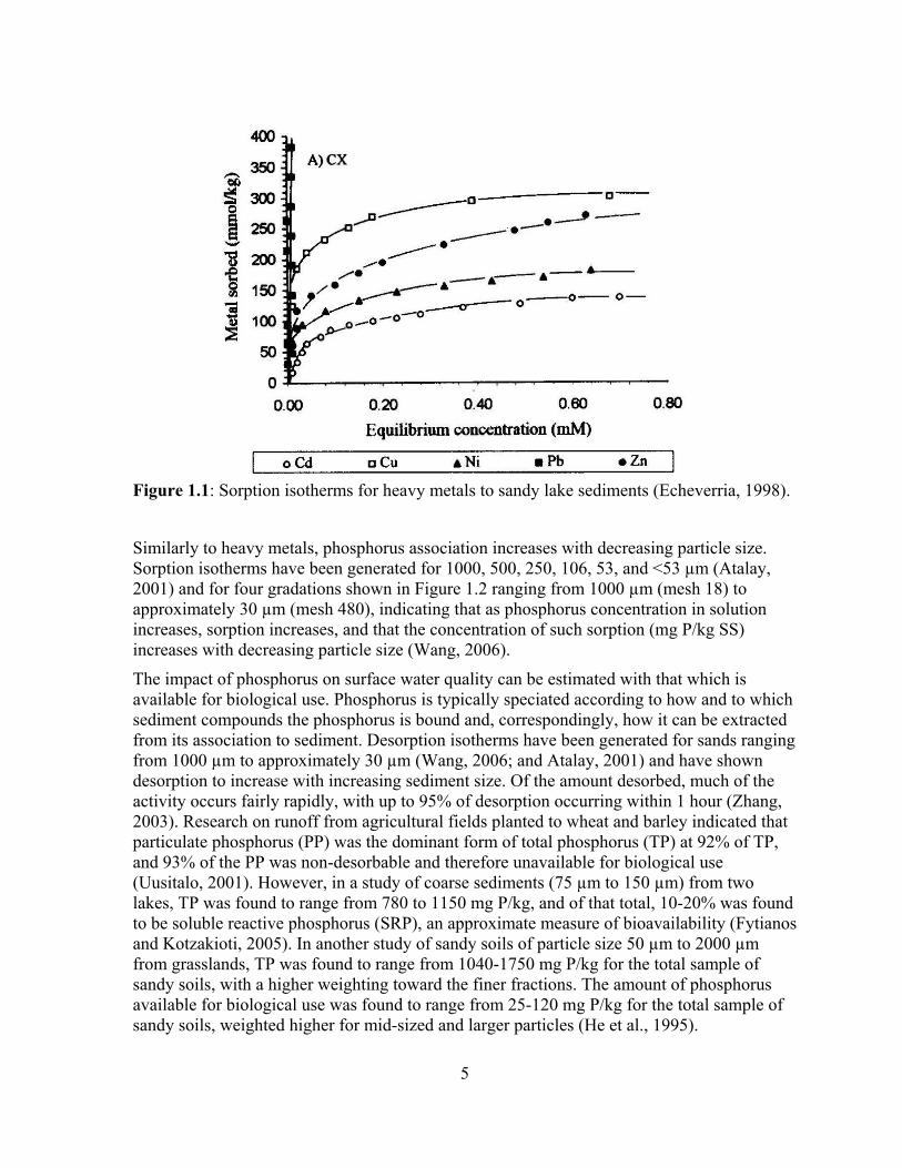
Figure 1.1 depicts sorption isotherms for several heavy metals onto a sandy soil. Clearly, as the equilibrium concentration is increased, sorption of each metal to sediment particles increases (Echeverria, 1998). The sorption increase is rapid for 0-0.2 millimolar (mM) concentration and plateaus at greater equilibrium concentrations, indicating that the active sorption sites are becoming scarce for this soil at concentrations above approximately 0.2 mM.
5
Figure 1.1: Sorption isotherms for heavy metals to sandy lake sediments (Echeverria, 1998).
Similarly to heavy metals, phosphorus association increases with decreasing particle size. Sorption isotherms have been generated for 1000, 500, 250, 106, 53, and <53 µm (Atalay, 2001) and for four gradations shown in Figure 1.2 ranging from 1000 µm (mesh 18) to approximately 30 µm (mesh 480), indicating that as phosphorus concentration in solution increases, sorption increases, and that the concentration of such sorption (mg P/kg SS) increases with decreasing particle size (Wang, 2006).
The impact of phosphorus on surface water quality can be estimated with that which is available for biological use. Phosphorus is typically speciated according to how and to which sediment compounds the phosphorus is bound and, correspondingly, how it can be extracted from its association to sediment. Desorption isotherms have been generated for sands ranging from 1000 µm to approximately 30 µm (Wang, 2006; and Atalay, 2001) and have shown desorption to increase with increasing sediment size. Of the amount desorbed, much of the activity occurs fairly rapidly, with up to 95% of desorption occurring within 1 hour (Zhang, 2003). Research on runoff from agricultural fields planted to wheat and barley indicated that particulate phosphorus (PP) was the dominant form of total phosphorus (TP) at 92% of TP, and 93% of the PP was non-desorbable and therefore unavailable for biological use (Uusitalo, 2001). However, in a study of coarse sediments (75 µm to 150 µm) from two lakes, TP was found to range from 780 to 1150 mg P/kg, and of that total, 10-20% was found to be soluble reactive phosphorus (SRP), an approximate measure of bioavailability (Fytianos and Kotzakioti, 2005). In another study of sandy soils of particle size 50 µm to 2000 µm from grasslands, TP was found to range from 1040-1750 mg P/kg for the total sample of sandy soils, with a higher weighting toward the finer fractions. The amount of phosphorus available for biological use was found to range from 25-120 mg P/kg for the total sample of sandy soils, weighted higher for mid-sized and larger particles (He et al., 1995).

6
Figure 1.2: Sorption isotherms for phosphorus to lake sediments, sorted by sediment size (from Wang, 2006) The geographic location of the watershed (and associated samples collected) directly influences precipitation patterns, rainfall intensity, rainfall duration, antecedent dry period, land uses, and soil types, which all factor into resultant metal concentrations (Barber, 2006), as well as phosphorus, in sediments.
Though very fine particles have been shown to make up the bulk number of particles in runoff, the bulk of particle mass often lies with coarser sediments. In a study of urban freeway runoff, more than 95% of the number of particles were smaller than 20 µm in diameter; but, these particles constituted less than 20% of the total mass. So, 80% of the mass of particles were larger than 20 µm, and more than 60% of the mass of particles were larger than 100 µm (Li, 2006). These results suggest that it may not be necessary to capture extremely fine particles (<20 µm) in order to reduce heavy metals and phosphorus pollutant loadings, even though on a concentration basis, the majority of heavy metals and phosphorus have been shown to associate with the finest grain sizes.
Thus, if a BMPs removal capability of a particular sediment size is known, and if an understanding of actual metal and phosphorus associations in a watershed of interest is lacking, a reasonable estimate of annual heavy metals removal could be estimated using conservative values from literature.
7
2. Methods and Materials
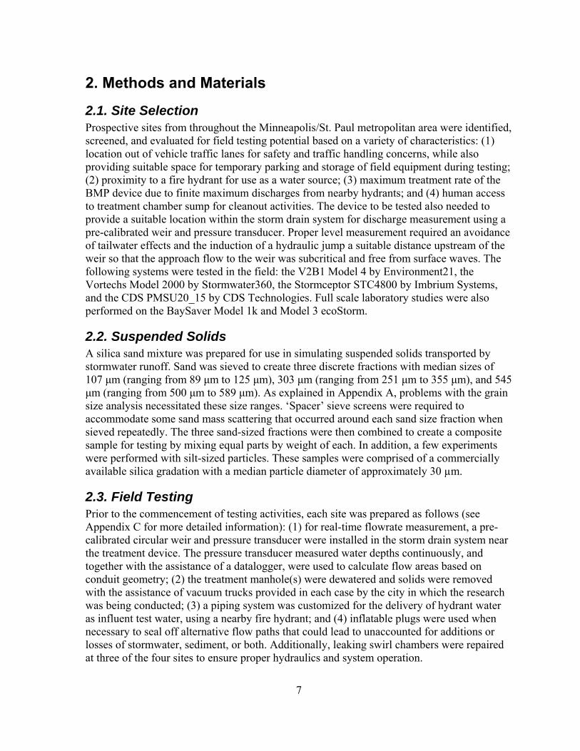
2.1. Site Selection Prospective sites from throughout the Minneapolis/St. Paul metropolitan area were identified, screened, and evaluated for field testing potential based on a variety of characteristics: (1) location out of vehicle traffic lanes for safety and traffic handling concerns, while also providing suitable space for temporary parking and storage of field equipment during testing; (2) proximity to a fire hydrant for use as a water source; (3) maximum treatment rate of the BMP device due to finite maximum discharges from nearby hydrants; and (4) human access to treatment chamber sump for cleanout activities. The device to be tested also needed to provide a suitable location within the storm drain system for discharge measurement using a pre-calibrated weir and pressure transducer. Proper level measurement required an avoidance of tailwater effects and the induction of a hydraulic jump a suitable distance upstream of the weir so that the approach flow to the weir was subcritical and free from surface waves. The following systems were tested in the field: the V2B1 Model 4 by Environment21, the Vortechs Model 2000 by Stormwater360, the Stormceptor STC4800 by Imbrium Systems, and the CDS PMSU20_15 by CDS Technologies. Full scale laboratory studies were also performed on the BaySaver Model 1k and Model 3 ecoStorm.
2.2. Suspended Solids A silica sand mixture was prepared for use in simulating suspended solids transported by stormwater runoff. Sand was sieved to create three discrete fractions with median sizes of 107 µm (ranging from 89 µm to 125 µm), 303 µm (ranging from 251 µm to 355 µm), and 545 µm (ranging from 500 µm to 589 µm). As explained in Appendix A, problems with the grain size analysis necessitated these size ranges. ‘Spacer’ sieve screens were required to accommodate some sand mass scattering that occurred around each sand size fraction when sieved repeatedly. The three sand-sized fractions were then combined to create a composite sample for testing by mixing equal parts by weight of each. In addition, a few experiments were performed with silt-sized particles. These samples were comprised of a commercially available silica gradation with a median particle diameter of approximately 30 µm.
2.3. Field Testing Prior to the commencement of testing activities, each site was prepared as follows (see Appendix C for more detailed information): (1) for real-time flowrate measurement, a pre-calibrated circular weir and pressure transducer were installed in the storm drain system near the treatment device. The pressure transducer measured water depths continuously, and together with the assistance of a datalogger, were used to calculate flow areas based on conduit geometry; (2) the treatment manhole(s) were dewatered and solids were removed with the assistance of vacuum trucks provided in each case by the city in which the research was being conducted; (3) a piping system was customized for the delivery of hydrant water as influent test water, using a nearby fire hydrant; and (4) inflatable plugs were used when necessary to seal off alternative flow paths that could lead to unaccounted for additions or losses of stormwater, sediment, or both. Additionally, leaking swirl chambers were repaired at three of the four sites to ensure proper hydraulics and system operation.
8
After each site and device were prepared for assessment, field testing commenced as follows:
1. the desired flowrate through the system was established using real time level measurements from a pressure transducer and datalogger, and conditioning the flow with a gate valve on the hydrant. The datalogger recorded 60-second average levels and provided an updated readout every second;
2. 10-15 kg of the sand test mixture was introduced to the influent hydrant water at 200 mg/L using a pre-calibrated sediment feeder. The total load varied depending on the magnitude of the flowrate; that is, at higher flowrates, in which removal performance was expected to be low, more sand was fed during a test to ensure a significant mass of sand was retained to reduce measurement error;
3. the water temperature, mass of solids delivered, and test duration were recorded;
4. following a 15 to 20 minute period to allow the sand particles to settle, the device was dewatered with sump pumps, and retained solids were removed from each manhole separately with a wet/dry vacuum;
5. the collected sediment was oven-dried and then sieved into the original size fractions, and each fraction was weighed.
The fractional removal of each sediment size fraction was computed by dividing the mass of sand in that size fraction retained by the treatment device during the test by the known quantity of sand in that size fraction delivered to the device. Each test produced three data points because three discrete sand size ranges were used. Each device was tested under four discharge conditions in triplicate, at approximately 25%, 50%, 75%, and 100% of the maximum treatment rate, for a total of 12 tests. Under ideal test conditions, the removal efficiency of each device would thus be described by 36 data points.
After conducting several tests, it was determined that some pollutant loading scenarios were difficult to simulate. For low flowrates, larger sand grains may settle to the bottom of the inlet pipe and not enter the treatment device. To minimize this problem, one or more of the following approaches were used: (1) increasing the minimum flow rate, (2) eliminating the largest sand size fraction, and (3) moving the sediment delivery point closer to the inlet of the device.
In many proprietary underground devices, pollutants are removed by two treatment chambers. As a result, sand is often retained in both the settling chamber as well as the floatables trap. Sand retained by the device during testing was collected and inventoried separately for each chamber.

9
3. Scaling and Removal Efficiency Based upon previous experience with settling of suspended sediments in lakes (Dhamotharan, et al., 1981), the Peclet number (Pe = Vs L /Dt) and a dimensionless time, were shown to be appropriate parameters explaining sediment deposition ratio, where Vs is particle settling velocity, L is settling depth, and Dt is the turbulent diffusion coefficient. Peclet number is defined as the ratio of advection to diffusion, where advective, settling forces are opposed by turbulent diffusion in the system tending to keep solids in suspension. Similar to the approach taken for lakes, advection here can be scaled with the settling velocity, Vs, times a settling length scale, h. Dt also scales with a velocity times a length scale, where the length scale is the shortest dimension of the flow. In many cases, the main dimensions of underground structures (diameter d and settling depth h) are similar. When the diameter is the shortest dimension of the flow, Dt ~ Ud, and by continuity Dt ~ Qd/A. In sedimentation devices, flow enters the chamber from above and turbulence is stronger where plunging occurs. Therefore, if A is taken as the horizontal projection of the chamber (the cross-sectional area of mixing) which is proportional to d2, then Dt ~Qd/d2 = Q/d and Pe = Vs.h.d/Q.
If the smallest dimension of the device is its height, or settling distance, as is the case for detention ponds, then inflow is relatively horizontal and thus A becomes the cross-section of the pond, hd. In both cases, one derives the same equation for the Peclet number. Therefore Dt ~Qh/dh = Q/d and Pe = Vs .h.d/Q.
If a different length scale is used, we get the Hazen number, which is the ratio of settling velocity to overflow rate and which can also be written as Vs d2/Q. The Peclet number can also be expressed as a function of residence time, Vs.hd/Q = (Vs/d)/(Q/hd2) = Vstr/d without considering turbulent diffusion or mixing.
The dimensional analysis performed to derive the Peclet number depends upon three primary assumptions, two of which were tested and verified with field and laboratory experiments, as follows:
1. Settling velocity. Based on the conclusions drawn by Fentie et al. (2004) in a study comparing multiple soil particle settling formulae versus measured settling data, velocity was assumed to follow the Cheng formula (1997) (Equation 1). The Cheng formula was shown to outperform other settling models, and is an explicit relationship for settling of natural sand particles derived from the particle Reynolds number (Re) and a dimensionless particle parameter. It is applicable to a wide range of Re, from the Stokes flow to turbulent regimes.
512
31
2 52125
.
s
s
gD.
DV
⎟⎟⎟⎟⎟⎟
⎠
⎞
⎜⎜⎜⎜⎜⎜
⎝
⎛
−
⎟⎟⎟⎟⎟
⎠
⎞
⎜⎜⎜⎜⎜
⎝
⎛
⎟⎟⎟⎟
⎠
⎞
⎜⎜⎜⎜
⎝
⎛ −
+=νρρρ
ν (1)
where Vs is particle settling velocity, ν is kinematic viscosity of the fluid, D is particle diameter, g is the gravity constant, ρs is particle density, and ρ is fluid density.
10
Stokes Law assumes an equivalent spherical particle shape and approximates settling velocity of sands with a particle Reynolds number of less than about 3 (sands up to approximately 175 µm in diameter). Settling velocity for larger particles can be estimated using a drag coefficient which is Reynolds number dependent (ASCE, 1975). Models were created to evaluate the differences in resultant removal efficiencies when settling was approximated by Stokes Law for all particles, the combination of Stokes (small particles) and the Re-dependent drag coefficient (large particles), and finally using the Cheng formula for all particles. When an entire particle size distribution at a particular flow rate was routed through each of the models, the resultant removal efficiencies were all within approximately 1.6%. While Stokes Law appears to adequately represent particle settling behavior for the particles and devices tested in this research, Stokes Law may not work for all systems.
2. Scaling with Pe. It is assumed that the mixing dynamics, and therefore the removal efficiency, scales with size (i.e. diameter and depth) for each particular device. This assumption was verified via laboratory experiments in which: (a) the diameter of the primary sedimentation manhole in a BaySaver Model 1k was increased and (b) the depth of a Model 3 ecoStorm was decreased by inserting a temporary false floor. The removal efficiencies for both modified devices, however, still plotted on the original performance curves (Carlson et al., 2006; Mohseni and Fyten, 2007). This behavior has powerful implications for the use of performance curves not only as an evaluator of existing underground device installations, but also as a primary tool for accurately sizing new devices of the same design.
Finally, the turbulent diffusion coefficient Dt is assumed to scale with Q/d across the range of flow rates evaluated. This assumption, made on dimensional grounds, could not be tested in the highly turbulent flow of these devices.

11
4. Results Performance curves were developed for six underground devices. Two devices were tested in the laboratory and four devices were tested in the field. Because the ecoStorm and Stormceptor units are single manhole treatment systems, only one performance curve was generated for each device. For the remaining two-chamber devices, performance curves were generated for the settling chamber (termed “primary”) and for the combination of the settling and floatables-trap chambers (termed “total removal”). The dimensions from the settling chamber, h and d, were used in the Peclet number for both the settling chamber and total removal data sets. It is possible that including sediments retained in the floatables trap may be an overestimation of the removal capability of a device because the floatables-trapping manholes use underflow baffle walls that may lead to resuspension of settled solids, especially at higher flow rates. Since tests were conducted in triplicate for each flowrate, a normalized range (range/mean) was calculated in order to assess the repeatability of each experiment. The normalized ranges varied from 0.6% to 15.6%, with a mean of 5.8%. This variation is small, compared to the accuracy typical of field measurements on stormwater treatment facilities (Weiss et al., 2007). Much of the variability can be attributed to slightly different experimental conditions during replicate tests. In some cases, flow rates differed by as much as 13%, and in others there were small but unavoidable differences in water temperature (up to 2.5°C) , which influences particle settling velocity. Changes in flow rate or temperature produce different Peclet numbers, which in turn produce different removal efficiencies.
The sediment removal performance for the six devices decreased towards zero with decreasing Peclet numbers (Figures 4.1 to 4.7). For a given device with fixed length scales h and d, a low Peclet number can result from a low settling velocity, Vs, as well as from a high flow rate, Q. Not surprisingly, all devices removed sediment more successfully at higher Peclet numbers. Ideally, as the length scales become smaller, the removal efficiency would decrease as well. Conversely, as the length scales increase the removal efficiency should asymptotically approach 1 (i.e. 100%). Since tests were conducted in triplicate for each flowrate, coefficients of variation were calculated in order to assess the repeatability of the experiment. A three parameter, exponential function of Peclet number (Equation 2) was fit to the solids removal results obtained for each device. This particular function was chosen due to its ability to correctly capture the concavity of the trend, and its tendency toward zero as Peclet number approaches zero and toward 1 as Peclet number approaches infinity. A non-linear regression analysis was performed on each dataset to identify each of the three parameters.
b
bb (aPe)Rη
1
11−
⎟⎟⎠
⎞⎜⎜⎝
⎛+= (2)
where η is the removal efficiency, R is the removal as Pe approaches infinity, a is a measure of the initial slope of the curve at Pe = 0, the exponent b is a measure of the curvature in the function at R = aPe, i.e. the intersection of two asymptotes (η = aPe and η = R) and Pe is the independent dimensionless variable. The parameter R was limited to positive values less than
12
or equal to unity since removal efficiency cannot exceed 100%. As b ∞, the curve becomes the lesser value of the two asymptotes. That is, as b ∞, at values of Pe less than R/a, η = aPe, and at values of Pe greater than R/a, η = R.
The Nash-Sutcliffe Coefficient (NSC) (Equation 3) was tabulated for each data set as a measure of how well the fitted function in Equation 2 describes the dataset, relative to how well the mean value describes the same data set.
2
2
1)yy(
)yy(NSC
imeasmeas
iimeas
−∑
∑ −−= (3)
where ymeasi is the measured removal data point for a given Pe, yi is the fitted value from Equation 1 for the same Pe, and measy is the dataset’s mean measured removal.
The root mean squared error (RMSE) (Equation 4) was also tabulated for each dataset as another measure of the goodness of fit of Equation 2 relative to the measured data.
pn)yy(
RMSE imeasi
−∑ −
=2
(4)
where n is the number of observations and p is the number of parameters in the fitted function. Thus, RMSE is the average vertical variation from the measured data point to the fitted function.
The performance functions for the BaySaver model 1k are the results of testing at St. Anthony Falls Laboratory in 2005 and early 2006. The BaySaver was subjected to a relatively narrowly graded particle size distribution (F95) with a median particle diameter of approximately 125 µm. A modified version of this device was also tested, and the results are shown in Figures 4.1 and 4.2. The size of the settling chamber manhole was increased from 1.22 m (4 ft) to 1.83 m (6 ft) and the removal efficiency from tests on the 1.83 m (6 ft) chamber plotted on the same function as for the 1.22 m (4 ft) chamber. Figure 4.1 provides some context for the interpretation of the parameter a of the fitted function, i.e. the initial slope of the portion of the curve, at Pe = 0, and for the exponent b, i.e. the curvature at R=aPe. Figure 4.2 provides a broader view of the Peclet numbers produced from the solids size distribution and discharges typical of these underground structures.

13
0.0
0.1
0.2
0.3
0.4
0.5
0.6
0.7
0.8
0.9
1.0
0 1 2 3 4Pe
Rem
oval
effi
cien
cy, η
primary measured-PM=1.2m primary measured-PM=1.8mtotal measured-PM=1.2m total measured-PM=1.8m
NSC=0.87RMSE=4.1%
NSC=0.99RMSE=3.8%
Total
Primary0.62
1
0.620.62 (1.77Pe)1
0.741η
−
⎟⎟⎠
⎞⎜⎜⎝
⎛+=
1.221
1.22(2.02Pe)11η
−
⎟⎟⎠
⎞⎜⎜⎝
⎛+=
Figure 4.1: Removal efficiency versus Pe for the new BaySaver Model 1k in rectangular coordinates (after Carlson et al., 2006)
0.0
0.1
0.2
0.3
0.4
0.5
0.6
0.7
0.8
0.9
1.0
0.1 1.0 10.0Pe
Rem
oval
effi
cien
cy, η
primary measured-PM=1.2m primary measured-PM=1.8mtotal measured-PM=1.2m total measured-PM=1.8m
NSC=0.87RMSE=4.1%
Primary
0.621
0.620.62 (1.77Pe)1
0.741η
−
⎟⎟⎠
⎞⎜⎜⎝
⎛+=
NSC=0.99RMSE=3.8%
1.221
1.22(2.02Pe)11η
−
⎟⎟⎠
⎞⎜⎜⎝
⎛+=
Figure 4.2: Removal efficiency versus Pe for the BaySaver Model 1k (after Carlson et al., 2006). The data and performance function for the Model 3 ecoStorm, tested at St. Anthony Falls Laboratory in the summer and fall 2006, are shown in Figure 4.3. The ecoStorm was evaluated when loaded with the test sand mixture described in section 2. This device height

14
was modified with a temporary false floor to assess its performance when the settling depth was altered (Mohseni and Fyten, 2007). The results with the modified chamber dimension are included in Figure 4.3.
0.0
0.1
0.2
0.3
0.4
0.5
0.6
0.7
0.8
0.9
1.0
0.1 1.0 10.0
Pe
Rem
oval
effi
cien
cy, η
measured measured with false floor fit
NSC=0.96RMSE=6.6%
4.151
4.154.15 (1.07Pe)1
0.991η
−
⎟⎟⎠
⎞⎜⎜⎝
⎛+=
Figure 4.3: Removal efficiency of the Model 3 ecoStorm versus Pe (from Mohseni and Fyten, 2007).
The data and performance functions for the field-tested Environment21 V2B1 Model 4 are shown in Figure 4.4. This device was installed in the summer of 2005. Flow rates tested were approximately 0.017 cms (0.6 cfs), 0.021 cms (0.75 cfs), 0.030 cms (1.05 cfs), and 0.040 cms (1.4 cfs), which correspond to 43%, 53%, 75%, and 100% of the maximum treatment rate, respectively. Clearly, the results are consistent with the general trend of better removal at higher Peclet number. If the results are extrapolated to low Peclet numbers, one would expect that the V2B1 would not be as effective at removing finer particles such as silts and clays. This hypothesis was verified with two tests conducted with silt-sized particles, with a median particle diameter of approximately 30 µm. Tests with this particle size produced a Peclet number of 0.03, and correspondingly low removal efficiency. Total removal efficiencies approach 98% for larger Peclet numbers.
15
0.00.10.20.30.40.50.60.70.80.91.0
0.01 0.10 1.00 10.00Pe
Rem
oval
Effi
cien
cy, η
primary measured total measured primary fit total fit
NSC=0.98RMSE=3.1%
NSC=0.99RMSE=2.1%
Primary
Total
2.361
2.362.36 (1.06Pe)1
0.741η
−
⎟⎟⎠
⎞⎜⎜⎝
⎛+=
1.851
1.851.85 (2.20Pe)1
0.991η
−
⎟⎟⎠
⎞⎜⎜⎝
⎛+=
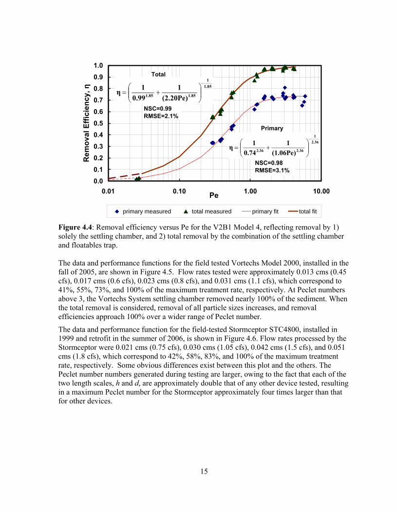
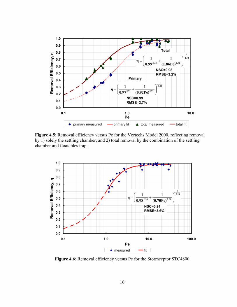
Figure 4.4: Removal efficiency versus Pe for the V2B1 Model 4, reflecting removal by 1) solely the settling chamber, and 2) total removal by the combination of the settling chamber and floatables trap. The data and performance functions for the field tested Vortechs Model 2000, installed in the fall of 2005, are shown in Figure 4.5. Flow rates tested were approximately 0.013 cms (0.45 cfs), 0.017 cms (0.6 cfs), 0.023 cms (0.8 cfs), and 0.031 cms (1.1 cfs), which correspond to 41%, 55%, 73%, and 100% of the maximum treatment rate, respectively. At Peclet numbers above 3, the Vortechs System settling chamber removed nearly 100% of the sediment. When the total removal is considered, removal of all particle sizes increases, and removal efficiencies approach 100% over a wider range of Peclet number.
The data and performance function for the field-tested Stormceptor STC4800, installed in 1999 and retrofit in the summer of 2006, is shown in Figure 4.6. Flow rates processed by the Stormceptor were 0.021 cms (0.75 cfs), 0.030 cms (1.05 cfs), 0.042 cms (1.5 cfs), and 0.051 cms (1.8 cfs), which correspond to 42%, 58%, 83%, and 100% of the maximum treatment rate, respectively. Some obvious differences exist between this plot and the others. The Peclet number numbers generated during testing are larger, owing to the fact that each of the two length scales, h and d, are approximately double that of any other device tested, resulting in a maximum Peclet number for the Stormceptor approximately four times larger than that for other devices.
16
0.0
0.1
0.2
0.3
0.4
0.5
0.6
0.7
0.8
0.9
1.0
0.1 1.0 10.0Pe
Rem
oval
Effi
cien
cy, η
primary measured primary fit total measured total fit
NSC=0.99RMSE=2.7%
Primary
NSC=0.98RMSE=3.2%
Total
2.711
2.712.71 (0.92Pe)1
0.971η
−
⎟⎟⎠
⎞⎜⎜⎝
⎛+=
2.321
2.322.32 (1.86Pe)1
0.991η
−
⎟⎟⎠
⎞⎜⎜⎝
⎛+=
Figure 4.5: Removal efficiency versus Pe for the Vortechs Model 2000, reflecting removal by 1) solely the settling chamber, and 2) total removal by the combination of the settling chamber and floatables trap.
0.0
0.1
0.2
0.3
0.4
0.5
0.6
0.7
0.8
0.9
1.0
0.1 1.0 10.0 100.0Pe
Rem
oval
Effi
cien
cy, η
measured fit
NSC=0.91RMSE=3.6%
2.281
2.282.28 (0.70Pe)1
0.981η
−
⎟⎟⎠
⎞⎜⎜⎝
⎛+=
Figure 4.6: Removal efficiency versus Pe for the Stormceptor STC4800
17
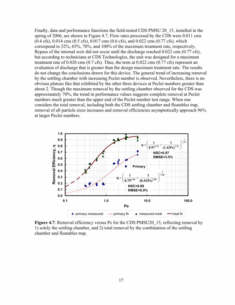
Finally, data and performance functions the field-tested CDS PMSU 20_15, installed in the spring of 2006, are shown in Figure 4.7. Flow rates processed by the CDS were 0.011 cms (0.4 cfs), 0.014 cms (0.5 cfs), 0.017 cms (0.6 cfs), and 0.022 cms (0.77 cfs), which correspond to 52%, 65%, 78%, and 100% of the maximum treatment rate, respectively. Bypass of the internal weir did not occur until the discharge reached 0.022 cms (0.77 cfs), but according to technicians at CDS Technologies, the unit was designed for a maximum treatment rate of 0.020 cms (0.7 cfs). Thus, the tests at 0.022 cms (0.77 cfs) represent an evaluation of discharge that is greater than the design maximum treatment rate. The results do not change the conclusions drawn for this device. The general trend of increasing removal by the settling chamber with increasing Peclet number is observed. Nevertheless, there is no obvious plateau like that exhibited by the other three devices at Peclet numbers greater than about 2. Though the maximum removal by the settling chamber observed for the CDS was approximately 70%, the trend in performance values suggests complete removal at Peclet numbers much greater than the upper end of the Peclet number test range. When one considers the total removal, including both the CDS settling chamber and floatables trap, removal of all particle sizes increases and removal efficiencies asymptotically approach 96% at larger Peclet numbers.
0.0
0.1
0.2
0.3
0.4
0.5
0.6
0.7
0.8
0.9
1.0
0.1 1.0 10.0 100.0Pe
Rem
oval
Effi
cien
cy, η
primary measured primary fit measured total total fit
NSC=0.89RMSE=6.9%
Primary
NSC=0.97RMSE=3.5%
1.481
1.481.48 (0.41Pe)1
0.751η
−
⎟⎟⎠
⎞⎜⎜⎝
⎛+=
1.751
1.751.75 (1.42Pe)1
0.971η
−
⎟⎟⎠
⎞⎜⎜⎝
⎛+=
Figure 4.7: Removal efficiency versus Pe for the CDS PMSU20_15, reflecting removal by 1) solely the settling chamber, and 2) total removal by the combination of the settling chamber and floatables trap.

18

19
5. Discussion The results of this research indicate that controlled field testing is a viable alternative to field monitoring. Field testing presents some site selection constraints in comparison to monitoring that need to be overcome, as outlined in the site selection section. Logistically, controlled field testing may be more intensive and laborious than monitoring, requiring working around the inconveniences of an in situ system, such as baseflow in the system, leaking chambers, challenging hydraulics, etc. However, field testing offers the potential for significant advantages in productivity and cost efficiency compared to monitoring. More importantly, the advantages offered by controlled field testing in terms of accuracy and repeatability of suspended solids removal capability cannot be understated.
These findings present evidence that Peclet number can be used to determine removal efficiency of a given device under various operating conditions, such as discharge and solids loading. In addition, removal efficiency seems to be maintained on the same function after changing the length scales within some limits. Many of the devices tested seem to approach a plateau in removal efficiency at Peclet numbers of about 2, where further increases in the size of the device have a reduced impact on performance. Thus, a Pe value of 2 may be a cost-effective target for sizing underground proprietary devices. It may be inappropriate to make direct comparisons of the performance of individual devices tested in this work because they were designed and installed at different times and may represent different generations of underground sedimentation devices in this continually evolving field.

20

21
6. Application of Results Performance curves can not only be used to make a prediction about the expected removal capability of a particular type of underground structure, but can also be utilized as a primary tool in the accurate sizing of new underground installations. As a starting point, minimum length scales may be roughly estimated using fixed inputs to a removal efficiency versus Peclet number relationship. Assumptions can be made regarding a target particle size in the stormwater runoff, and therefore Vs, as well as a flow rate, Q, such that length scales, h and d can be derived for a desired Peclet number.
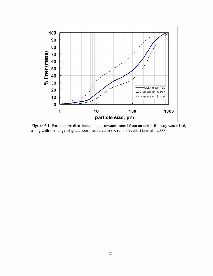
In a simple example, a target particle size to be removed can be estimated using the median diameter from a sample mean particle size distribution (PSD) contained in urban roadway runoff (Li et al., 2005), as shown in Figure 6.1. The D50 is approximately 120 µm, which produces a settling rate of approximately 0.008 m/s (0.027 ft/s), using the Cheng formula for 20°C water and assumed particle density (ρs = 2.65 g/cm3). Assuming a flowrate of 0.051 cms (1.8 cfs) from a hypothetical watershed and a desired Peclet number of 2, the only unknown in the Peclet number equation (Pe=Vs.h.d/Q) will be the product of length scales, h and d, which in this case is approximately 12.2 m2 (130 ft2). The Stormceptor Model STC7200, with h and d of 3.4 m (11.2 ft) and 3.7 m (12 ft), respectively, provides the smallest product of length scales greater than 12.2 m2 (130 ft2). Using the performance function in Figure 4.6, the predicted removal efficiency of 120 µm particles was approximately 84%.
When the entire particle size distribution in Figure 6.1 is routed through the performance function in Figure 4.6 at a constant concentration, and assuming the constant flow rate of 1.8 cfs, and length scales 3.4 m (11.2 ft) and 3.7 m (12 ft) for h and d, respectively, the removal efficiency becomes approximately 57%.
An actual sizing exercise requires a removal efficiency target be set based on regulatory agency thresholds. A hydrologic analysis is also required to generate a representative hydrograph that is specific to the watershed. The representative hydrograph, together with an entire, representative particle size distribution contained in the stormwater runoff, produces an annual solids loading which can be routed through a performance function to derive minimum length scales that will satisfy the specified criteria.
22
0102030405060708090
100
1 10 100 1000particle size, µm
% fi
ner (
mas
s)
UCLA mean PSDminimum % finermaximum % finer
Figure 6.1: Particle size distribution in stormwater runoff from an urban freeway watershed, along with the range of gradations measured in six runoff events (Li et al., 2005)

23
7. Conclusions and Recommendations The removal efficiency of proprietary underground stormwater treatment devices depends upon the settling velocity of influent solids, i.e., solid size and density, in addition to the size and hydraulic design of the device. A Peclet number that relates two length scales and particle settling velocity to influent flowrate, Pe=Vs.h.d/Q, was developed and shown to describe the settling capability of each device. The use of this parameter allows for a device’s performance to be predicted over a wide range of underground structure model sizes, storm events, and pollutant size characteristics. More tests should be conducted to investigate the specific behavior of proprietary underground structures when subjected to flows higher than the device’s maximum treatment rate.
In addition to predicting removal capabilities of existing installations, performance functions can serve as a tool in accurately sizing new installations. A designer can specify an appropriate runoff hydrograph for the watershed to be treated, identify a representative particle size distribution contained in the stormwater runoff, and choose length scales that satisfy regulatory requirements.
This research has shown that controlled field tests are a practical, robust and accurate means of determining an underground device’s performance, based upon the solid size distribution and density of the influent, in addition to the water discharge and temperature. It has been successfully verified on four devices in field tests, and two devices in laboratory tests. The protocol and results of testing will be a useful tool for consultants, manufacturers, local governments, and state agencies for selecting, sizing, and evaluating stormwater treatment technologies to protect water resources.

24

25
8. References American Society of Civil Engineers (ASCE). (1975). Sedimentation Engineering. ASCE
Manuals and Reports on Engineering Practice-No. 54, Washington D.C..
American Society of Testing and Materials (ASTM). (2005). Annual Book of ASTM Standards. C-136-05 Standard Test Method for Sieve Analysis of Fine and Coarse Aggregates. West Conshohocken, PA.
Andoh, R.Y.G. and A.J. Saul (2003). The use of hydrodynamic vortex separators and screening systems to improve water quality. Water Science and Technology, v 47, no 4, p 175-183.
Atalay, A. (2001). “Variation in phosphorus sorption with soil particle size.” Soil and sediment contamination, v 10, n 3, p 317-335.
Barber, M.E., M.G. Brown, K.M. Lingenfelder, and D.R. Yonge. (2006). Phase I: preliminary environmental investigation of heavy metals in highway runoff: final report. Washington State Transportation Center. November 21, Pullman, Washington. .
Barbosa, A.E. and T. Hvitved-Jacobsen. (1999). “Highway runoff and potential for removal of heavy metals in an infiltration pond in Portugal.” Science of the Total Environment, v 235, n 1, p 151-159.
Bonestroo, Rosene, Anderlik and Associates, Inc. (2002). Walker Avenue V2B1 Performance. March 19. Roseville, Minnesota.
Bonestroo, Rosene, Anderlik and Associates, Inc. (2003). Walker Avenue V2B1 2001-2002 Performance Assessment. April 15. Roseville, Minnesota.
Bradl, H. B. (2004) “Adsorption of heavy metal ions on soils and soils constituents.” Journal of Colloid and Interface Science, v 277, n 1, Sep 1, p 1-18.
Carlson, L., Mohseni, O., H. Stefan, and M. Lueker. (2006). Performance Evaluation of the BaySaver Stormwater Separation System. St Anthony Falls Laboratory, Project Report No. 472. University of Minnesota, Minneapolis, Minnesota.
CDS Technologies, Inc. 2006. Project design worksheets. Project no. MN-05-019, Minneapolis, MN.
Cheng, N.S. (1997). “A simplified settling velocity formula for sediment particle.” Journal of hydraulic engineering, ASCE, 123(2), 149-152.
CONTECH Stormwater Solutions: Vortechs. (2007) CONTECH Construction Products, Inc. <http://www.contech-cpi.com/media/assets/asset/file_name/ 3853/STD2k.dwg/>. May 25.

26
Dhamotharan, S., J.S. Gulliver and H.G. Stefan. (1981). Unsteady One-Dimensional Settling of Suspended Sediment. Water Resources Research, v 17, n 4, p 1125-1132.
Echeverria, J.C., M.T. Morera, C. Mazkiaran, J.J. Garido. (1998). “Competitive sorption of heavy metal by soils: isotherms and fractional factorial experiments.” Environmental Pollution, v 101, n 2, p 275-284.
England, G. (2001). Success stories of Brevard County, Florida stormwater utility. Journal of Water Resources Planning and Management, vl 127, v 3, May/June.
Environment21. (2005). Project design worksheets. Project: Rice Creek Road Area 4, .
Environmental Technology Verification (ETV). (2005a). ETV Report: BaySaver Separation System, model 10k. 05/21/WQPC-WWF, EPA/600/R-05/113, September, Ann Arbor, MI..
Environmental Technology Verification (ETV). (2005b). ETV Report: Vortechs System, model 1000. 05/24/WQPC-WWF, EPA/600/R-05/140, September, Ann Arbor, MI..
Fassman, E.A. (2006). Improving effectiveness and evaluation techniques of stormwater best management practices. Journal of Environmental Science And Health Part. 41: 1247-1256.
Fentie, B., B. Yu, and C.W. Rose. (2004). “Comparison of seven particle settling velocity formulae for erosion modeling.” 13th International Soil Conservation Organisation Conference, ISCO, Brisbane, Australia, 1-3.
Fytianos, K. and A. Kotzakioti. (2005). “Sequential fractionation of phosphorus in lake sediments of northern Greece.” Environmental Monitoring and Assessment. 100: 191–200.
German, J. and G. Svensson. (2002). “Metal content and particle size distribution of street sediments and street sweeping waste”. Water Science and Technology, v 46, n 6–7, p 191–198.
He, Z.L.; M.J. Wilson, C.O. Campbell, A.C. Edwards, and S.J. Chapman. (1995). “Distribution of phosphorus in soil aggregate fractions and its significance with regard to phosphorus transport in agricultural runoff.” Water, Air and Soil Pollution, v 83, n 1-2, p 69-84.
Huang, S. and Z. Wan. (1997). “Concurrent sorption of heavy metal pollutants of sediment of different grain sizes.” Journal of Hydrodynamics, v 9, n 1, p 1-12.
Johnson, P.D., S. Clark, R. Pitt, S.R. Durrans, M. Urritia, S. Gill, and J. Kirby. (2003) “Metals removal technologies for stormwater.” Proccedings of the Industrial Water Conference, WEF. San Antonio, TX.

27
Lau, S.-L., and M.K. Stenstrom (2005). “Metals and PAHs adsorbed to street particles”. Water Research, v 39, p 4083-4092.
Li, Y., S.-L. Lau, M. Kayhanian, and M. K. Stenstrom. (2006). “Dynamic Characteristics of Particle Size Distribution in Highway Runoff: Implications for Settling Tank Design.” Journal of Environmental Engineering, v 132, n 8, Aug 1.
Li, Y., S.-N. Lau, M. Kayhanian, and M.K. Stenstrom. (2005). Particle size distribution in highway runoff. Journ. of Environmental Engineering. v 131, n 9, September 1.
Mohseni, O. and A. Fyten (2007). Performance Assessment of ecoStorm™ for Removing Suspended Sediments from Stormwater. St Anthony Falls Laboratory, Project Report No. 495. University of Minnesota, Minneapolis, Minnesota.
New Jersey Corporation for Advanced Technology (NJCAT). (2004). NJCAT Technology Verification, BaySaver Technologies, Inc. Decembe, Trenton, NJ r.
Phillips, I.R. (1999). “Copper, lead, cadmium, and zinc sorption by waterlogged and air-dry soil.” Soil and Sediment Contamination, v 8, n 3, p 343-364.
Pitt, R., S. Clark, P.D. Johnson, R. Morquecho, S. Gill, and M. Pratap. (2004). “High level treatment of stormwater heavy metals.” Proceedings of the 2004 World Water and Environmental Resources Congress: Critical Transitions in Water and Environmental Resources Management, Jun 27-Jul 1 2004, Salt Lake City, UT, p 917-926.
Roger, S., M. Montrejaud-Vignoles, M.C. Andal, L. Herremans, and J.P. Fortune. (1998). “Mineral, physical, and chemical analysis of the solid matter carried by motorway runoff water.” Water Research, v 32, n 4, p 1119-1125.
Roseen, R.M., T.P. Ballestero, J.J. Houle, and P. Avelleneda. (2005). “Normalized technology verification of structural BMPs, Low Impact Development (LID) designs, and manufactured BMPs”. Proceedings of the Watershed Management Symposium. Williamsbug, VA.
Sa, S.-H., T. Masuda, and Y. Hosoi. (2005) “A study of SS size distribution during runoff and fractionation of phosphates depending on soil size in agricultural watershed.” Water Science and Technology, v 51, n 3-4, p 393-400.
Sansalone, J.J. and Buchberger, S.G. (1995). “Infiltration device as a best management practice for immobilizing heavy metals in urban highway runoff.” Water Science and Technology, v 32, n 1, p 119-125.
Schwarz, T. and S. Wells. (1999). “Continuous deflective separation of stormwater particulates”. Advances in Filtration and Separation Technology, v 12, p 219-226.

28
Soltan, M.E., M.N. Rashed, and G.M. Taha. (2001). “Heavy metal levels and adsorption capacity of Nile river sediments”. International Journal of Environmental Analytical Chemistry, v 80, n 3, p 167-186.
Stormceptor. (2007). Rinker Group, Ltd. <http://www.rinkerstormceptor.com/technicalinformation/drawing/>. May 25.
Strynchuk, J., J. Royal, and G. England. (2000). “Continuous deflective separation (CDS) unit for sediment control in Brevard County, Florida”. Proceedings of the Watershed Management Symposium. Fort Collins, CO.
Sutherland, R.A. (2003). “Lead in grain size fractions of road deposited sediment.” Environmental Pollution, v 121, p 229–237.
Tuccillo, M.E. (2006) “Size fractionation of metals in runoff from residential and highway storm sewers” Science of the Total Environment, v 355, p 288–300.
Uusitalo, R., Turtola, E., Kauppila, T., Lilja, T. (2001). “Particulate phosphorus and sediment in surface runoff and drainflow from clayey soils.”. Journal of Environmental Quality, v 30, n 2, p 589-595.
Wang, S., X. Jin, Q. Bu, X. Zhou, and F. Wu. (2006). “Effects of particle size, organic matter, and ionic strength on the phosphate sorption in different trophic lake sediments”. Journal of Hazardous Materials, v 128, n 2, p 95-105.
Waschbusch, R.J. (1999). Evaluation of the effectiveness of an urban stormwater treatment unit in Madison, Wisconsin, 1996-97. U.S.G.S. Water-Resources Investigations Report 99-4195. Middleton, Wisconsin.
Weiss, P., J.S. Gulliver, A.J. Erickson. (2007). Cost and pollutant removal of storm-water treatment practices. Journal of Water Resources Planning and Management, v 133, n 3, p 218-229.
Yu, S.L. and M.D.Stopinski. (2001). Testing of ultra-urban stormwater best management practices. VTRC 01-R7, Virginia Transportation ResearchCouncil: Charlottesville, VA, 1-43.
Zhang, M.K., Z.L He, D.V. Calvert, P.J. Stoffella, X.E. Yang, and Y.C. Li. (2003). “Phosphorus and heavy metal attachment and release in sandy soil aggregate fractions.” Soil Science Society of America Journal, v 67, n 4, July/August, p 1158-1167.
Zhu, T., T. Maelum, P.D. Jenssen, and T. Krogstad. (2003). “Phosphorus sorption characteristics of a light weight aggregate.” Water Science and Technology, v 48, n 5, p 93–100.

29
Appendix A: Sieving Operation

30
31
The grain size analysis of sediments used in field testing was of critical importance to the success of the performance characterization of proprietary underground structures. The ultimate objective was the development of a performance curve for each device, relating removal efficiency to a dimensionless parameter (see section 3). One of the variables in the dimensionless parameter is settling velocity, which is directly proportional to the square of particle diameter. So in order to develop an accurate performance curve, a good handle on particle size was paramount.
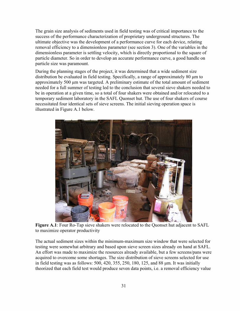
During the planning stages of the project, it was determined that a wide sediment size distribution be evaluated in field testing. Specifically, a range of approximately 80 µm to approximately 500 µm was targeted. A preliminary estimate of the total amount of sediment needed for a full summer of testing led to the conclusion that several sieve shakers needed to be in operation at a given time, so a total of four shakers were obtained and/or relocated to a temporary sediment laboratory in the SAFL Quonset hut. The use of four shakers of course necessitated four identical sets of sieve screens. The initial sieving operation space is illustrated in Figure A.1 below.
Figure A.1: Four Ro-Tap sieve shakers were relocated to the Quonset hut adjacent to SAFL to maximize operator productivity The actual sediment sizes within the minimum-maximum size window that were selected for testing were somewhat arbitrary and based upon sieve screen sizes already on hand at SAFL. An effort was made to maximize the resources already available, but a few screens/pans were acquired to overcome some shortages. The size distribution of sieve screens selected for use in field testing was as follows: 500, 420, 355, 250, 180, 125, and 88 µm. It was initially theorized that each field test would produce seven data points, i.e. a removal efficiency value
32
corresponding to each of the above seven sand sizes. However, as will be discussed below, problems subsequently developed that required a shift in strategy.
The design of the experiment called for an equivalent amount of sediment at each size interval. Since there is no commercially available sand mix with equal parts of the seven sizes above, a sand mix was instead created by the project team specifically for this work using three different commercially available sands as supply, blending them together, and separating them into the size ranges of interest by sieving. The three supply sands were AGSCO 35-50 with median particle diameter of approximately 425 µm, AGSCO 40-70 with median particle diameter of approximately 225 µm, and Sil-Co-Sil F110 with median particle diameter of approximately 110 µm. Each of these three sands has a fairly narrow size distribution; that is, they contain particle sizes in a relatively small range of sizes around the median diameter. Ninety percent of AGSCO 35-50 is within 300 and 500 µm, 77% of AGSCO 40-70 is within 210 and 420 µm, and 87% of F110 is within 75 and 200 µm. Thus, three commercial sands were necessary, and not just one or two, to populate the entire desired size distribution from 88 µm to 500 µm.
All sieving was completed in accordance with ASTM standards (ASTM, 2005) and required the full time attention of a SAFL student employee during the summer months. Ro-Tap style shakers and 0.2 m (8 in) diameter brass sieve screens were utilized. At the conclusion of each run, pans were emptied into associated 18.9 L (5 gal) plastic buckets that were classified by particle diameter, i.e. a separate bucket was used for each of the seven particle sizes. The process was slow-going, since there is a finite capacity of the 0.2 m (8 in) screens (less than approximately 200 grams retained per screen) that limited productivity.
For the initial field tests, 1-2 kg of each of the seven separated sand sizes was designed to be run through the underground structure. One kilogram was considered the minimum mass to deliver to the device so as to minimize the errors associated with collecting small amounts of sand retained inside a device during a test. The exact amount selected was dependent upon the test flowrate and using the assumption that at lower flowrates, a device was expected to be relatively successful. Thus, a higher percentage of delivered mass should be retained, leading to a lesser amount necessary to be fed. Conversely, at higher flowrates, it was assumed a device would be less successful, i.e. would remove a lower percentage of sediment delivered, so more sand was fed to the device so as to ensure measurement errors were minimized. Therefore, for lower flowrates, a mass closer to 1 kg of each sand size was delivered (for a total of 7 kg), and at higher flowrates, a mass nearer 2 kg of each sand size was fed (for a total of 14 kg). Clearly, this was a significant amount of sediment to sieve prior to any testing, when one multiplied this number by 48 tests.
Before departing for field testing each day, the appropriate mass of each sand size was weighed on a calibrated balance. One or more tests were performed in the field and the sand retained in the device during each test was brought back to SAFL for oven-drying overnight. When suitably dry, the sediment samples were sieved in the same manner as before, with the exception that the mass retained on each screen was weighed on the balance and the mass recorded. In many cases, multiple runs through the sieve screens were required of a sample if the mass exceeded the capacity of the screen. Once recorded, the individual sizes were combined and stored in Ziploc freezer bags.
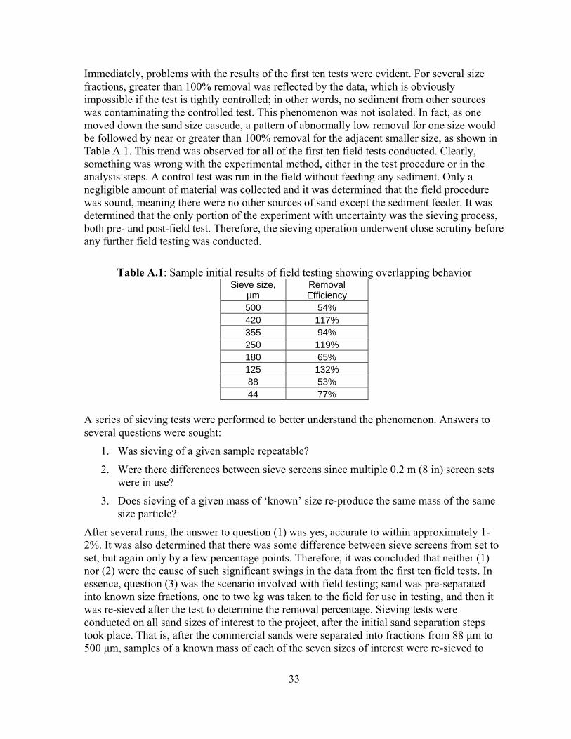
33
Immediately, problems with the results of the first ten tests were evident. For several size fractions, greater than 100% removal was reflected by the data, which is obviously impossible if the test is tightly controlled; in other words, no sediment from other sources was contaminating the controlled test. This phenomenon was not isolated. In fact, as one moved down the sand size cascade, a pattern of abnormally low removal for one size would be followed by near or greater than 100% removal for the adjacent smaller size, as shown in Table A.1. This trend was observed for all of the first ten field tests conducted. Clearly, something was wrong with the experimental method, either in the test procedure or in the analysis steps. A control test was run in the field without feeding any sediment. Only a negligible amount of material was collected and it was determined that the field procedure was sound, meaning there were no other sources of sand except the sediment feeder. It was determined that the only portion of the experiment with uncertainty was the sieving process, both pre- and post-field test. Therefore, the sieving operation underwent close scrutiny before any further field testing was conducted.
Table A.1: Sample initial results of field testing showing overlapping behavior
Sieve size, µm
Removal Efficiency
500 54% 420 117% 355 94% 250 119% 180 65% 125 132% 88 53% 44 77%
A series of sieving tests were performed to better understand the phenomenon. Answers to several questions were sought:
1. Was sieving of a given sample repeatable?
2. Were there differences between sieve screens since multiple 0.2 m (8 in) screen sets were in use?
3. Does sieving of a given mass of ‘known’ size re-produce the same mass of the same size particle?
After several runs, the answer to question (1) was yes, accurate to within approximately 1-2%. It was also determined that there was some difference between sieve screens from set to set, but again only by a few percentage points. Therefore, it was concluded that neither (1) nor (2) were the cause of such significant swings in the data from the first ten field tests. In essence, question (3) was the scenario involved with field testing; sand was pre-separated into known size fractions, one to two kg was taken to the field for use in testing, and then it was re-sieved after the test to determine the removal percentage. Sieving tests were conducted on all sand sizes of interest to the project, after the initial sand separation steps took place. That is, after the commercial sands were separated into fractions from 88 µm to 500 µm, samples of a known mass of each of the seven sizes of interest were re-sieved to

34
determine if the same mass of the same size sand could be retrieved. In each case, for each size analyzed, a significant percentage of the mass of a given particle size from the initial separation was retained on screens immediately adjacent (both larger and smaller) to the ‘correct’ screen. For example, for a given 200 g sample of 420 µm sand, much of the 200 g sample (~80%) would be retrieved from the 420 µm screen, but the remaining 20% would be distributed between the 500 µm and 355 µm screens. This pattern of scattering around the ‘correct’ size was witnessed for each of the seven sizes, though in different percentages, as illustrated in Table A.2 below.
Table A.2: Results of sieving analysis indicating scattering behavior around ‘correct’ size.
200g from carefully separated (ASTM method) 500micron bucket 589µm 500µm 420µm 355µm 250µm 180µm 125µm 88µm 44µm
#30 #35 #40 #45 #60 #80 #120 #170 #325 - 186.6 11.3 - - - - - -
200g from carefully separated (ASTM method) 420micron bucket 589µm 500µm 420µm 355µm 250µm 180µm 125µm 88µm 44µm
#30 #35 #40 #45 #60 #80 #120 #170 #325 - 26.6 164.1 6.1 - - - - -
200g from carefully separated (ASTM method) 355micron bucket 589µm 500µm 420µm 355µm 250µm 180µm 125µm 88µm 44µm
#30 #35 #40 #45 #60 #80 #120 #170 #325 - - 27.5 166.1 5.7 - - - -
200g from carefully separated (ASTM method) 250micron bucket 589µm 500µm 420µm 355µm 250µm 180µm 125µm 88µm 44µm
#30 #35 #40 #45 #60 #80 #120 #170 #325 - - - 11.7 181 5.2 - - -
200g from carefully separated (ASTM method) 180micron bucket 589µm 500µm 420µm 355µm 250µm 180µm 125µm 88µm 44µm
#30 #35 #40 #45 #60 #80 #120 #170 #325 - - - - 11.1 178 12.8 - -
200g from carefully separated (ASTM method) 125micron bucket 589µm 500µm 420µm 355µm 250µm 180µm 125µm 88µm 44µm
#30 #35 #40 #45 #60 #80 #120 #170 #325 - - - - - 2.2 157.6 39.2 -
200g from carefully separated (ASTM method) 88micron bucket 589µm 500µm 420µm 355µm 250µm 180µm 125µm 88µm 44µm
#30 #35 #40 #45 #60 #80 #120 #170 #325 - - - - - - 5.5 185 9.4
This observation explains why unusual size distributions were tabulated for the results of the first ten field tests. In addition, the scattering was shown to be limited to the immediately adjacent screens in all cases. Therefore, instead of testing seven different sizes, only three
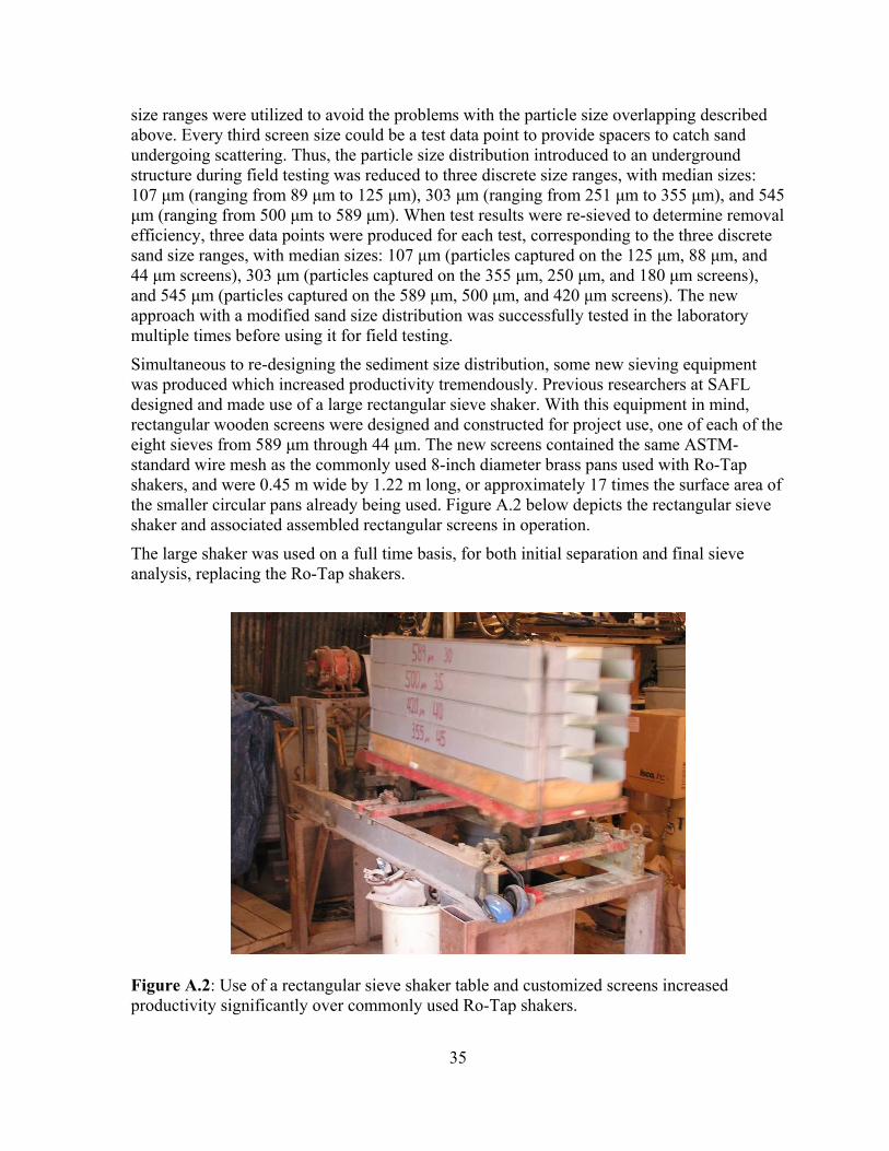
35
size ranges were utilized to avoid the problems with the particle size overlapping described above. Every third screen size could be a test data point to provide spacers to catch sand undergoing scattering. Thus, the particle size distribution introduced to an underground structure during field testing was reduced to three discrete size ranges, with median sizes: 107 µm (ranging from 89 µm to 125 µm), 303 µm (ranging from 251 µm to 355 µm), and 545 µm (ranging from 500 µm to 589 µm). When test results were re-sieved to determine removal efficiency, three data points were produced for each test, corresponding to the three discrete sand size ranges, with median sizes: 107 µm (particles captured on the 125 µm, 88 µm, and 44 µm screens), 303 µm (particles captured on the 355 µm, 250 µm, and 180 µm screens), and 545 µm (particles captured on the 589 µm, 500 µm, and 420 µm screens). The new approach with a modified sand size distribution was successfully tested in the laboratory multiple times before using it for field testing.
Simultaneous to re-designing the sediment size distribution, some new sieving equipment was produced which increased productivity tremendously. Previous researchers at SAFL designed and made use of a large rectangular sieve shaker. With this equipment in mind, rectangular wooden screens were designed and constructed for project use, one of each of the eight sieves from 589 µm through 44 µm. The new screens contained the same ASTM-standard wire mesh as the commonly used 8-inch diameter brass pans used with Ro-Tap shakers, and were 0.45 m wide by 1.22 m long, or approximately 17 times the surface area of the smaller circular pans already being used. Figure A.2 below depicts the rectangular sieve shaker and associated assembled rectangular screens in operation.
The large shaker was used on a full time basis, for both initial separation and final sieve analysis, replacing the Ro-Tap shakers.
Figure A.2: Use of a rectangular sieve shaker table and customized screens increased productivity significantly over commonly used Ro-Tap shakers.

36

37
Appendix B: Device Function Description

38
39
The design criteria, features, and functions of each underground sedimentation device tested in the field will be discussed in chronological order of testing, beginning with the V2B1 Model 4 device, followed by the Vortechs Model 2000, the Stormceptor Model STC4800, and finally the CDS Model PMSU20_15. The laboratory tests are described in Carlson et al. (2006) and Mohseni and Fyten (2007).
B.1. Environment21 V2B1 Model 4 The V2B1 Model 4, by Environment21, was installed in New Brighton, MN, at the intersection of Rice Creek Road and Long Lake Road. It receives stormwater runoff from a 1.7 ha (4.2 ac), residential watershed that is approximately 55% vegetated and 45% impervious. The V2B1 Model 4 is a dual manhole system, consisting of a 1.5 m (5 ft) diameter settling chamber and a five-foot diameter floatables trap. Stormwater influent is introduced tangentially to the settling chamber by a 0.38 m (15 in) PVC pipe, inducing a swirling motion inside the manhole. Relatively heavier particulates contained in the stormwater, such as sand, settle out of suspension in the settling chamber. Stormwater escapes the settling chamber by overflowing a 0.45 m (18 in) diameter PVC standpipe in the middle of the manhole, where the water is conveyed to the floatables trap. The floatables trap manhole contains an underflow baffle wall with a 0.3 m (1 ft) by 0.91 m (3 ft) rectangular hole at its base. Buoyant material (hydrocarbons, cigarette butts, some organic matter, etc) that passes through the settling chamber via the overflow standpipe are retained in the floatables trap because water must travel beneath the baffle wall to escape the system through a 0.38 m (15 in) PVC pipe. Downstream of the device, the effluent from the V2B1 discharges into a 36-inch storm drain pipe, which eventually empties into Long Lake. There is an overall drop of 0.06 m (0.2 ft) across the system, from the inlet invert to the outlet invert. The distance between pipe inverts and manhole inverts is approximately 1.4 m (4.5 ft) in each treatment manhole. One access point is provided to the settling chamber, and one access point on each side of the baffle wall in the floatables trap, as shown in Figure B.1.
The unit was designed to accommodate a maximum hydraulic flowrate equivalent to the 10-year event, with an intensity of 11.7 cm/hr (4.6 in/hr), without flooding the street. According to calculations provided by Environment21, this discharge is 0.19 cms (6.7 cfs), which serves as the capacity of the storm drain conveyance system around the device. The V2B1 is an in-line system with no bypass provided, meaning the device will receive all flows traveling through the system. However, even though all storm flows travel through the device, treatment is not intended to be provided above the water quality event, defined to be 2.0 cm (0.8 in) of rainfall. A runoff coefficient of 0.46 was estimated by the design engineer for the 1.7 ha (4.2 ac) watershed. According to calculations provided by Environment21, the water quality flowrate is 0.04 cms (1.37 cfs), which corresponds to the maximum treatment rate for performance assessment. The hydraulic conditions of the system produce a backwater condition inside the treatment manholes during a runoff event, which reduces the velocity in the inlet pipe. The advantage of slower velocities is that there is reduced mixing energy, meaning less opposition to settling. A disadvantage of low velocities is that it becomes difficult for all sediment, especially coarse particles, to remain in suspension in the inlet pipes under low and moderate flow rates. Therefore it is possible that under normal field operating conditions, the pipes upstream of the device will undergo sediment deposition,
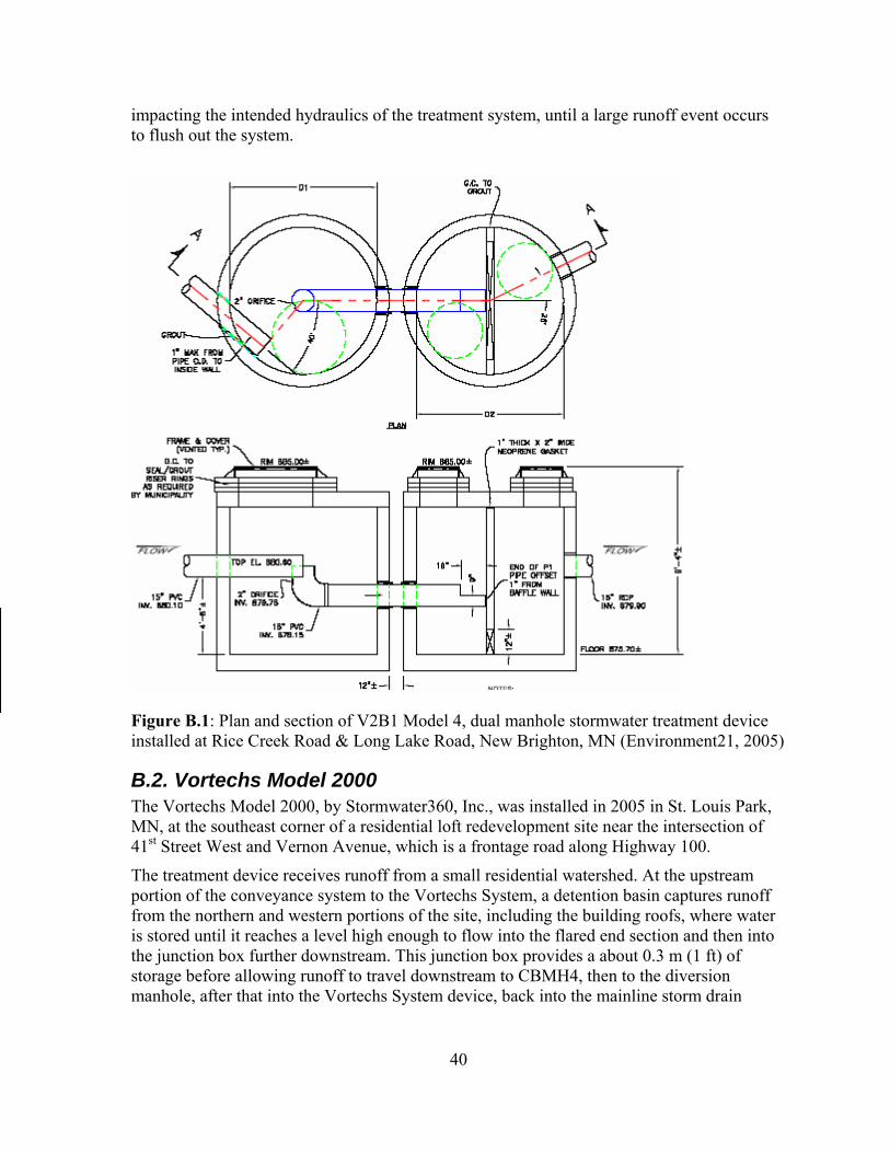
40
impacting the intended hydraulics of the treatment system, until a large runoff event occurs to flush out the system.
Figure B.1: Plan and section of V2B1 Model 4, dual manhole stormwater treatment device installed at Rice Creek Road & Long Lake Road, New Brighton, MN (Environment21, 2005)
B.2. Vortechs Model 2000 The Vortechs Model 2000, by Stormwater360, Inc., was installed in 2005 in St. Louis Park, MN, at the southeast corner of a residential loft redevelopment site near the intersection of 41st Street West and Vernon Avenue, which is a frontage road along Highway 100.
The treatment device receives runoff from a small residential watershed. At the upstream portion of the conveyance system to the Vortechs System, a detention basin captures runoff from the northern and western portions of the site, including the building roofs, where water is stored until it reaches a level high enough to flow into the flared end section and then into the junction box further downstream. This junction box provides a about 0.3 m (1 ft) of storage before allowing runoff to travel downstream to CBMH4, then to the diversion manhole, after that into the Vortechs System device, back into the mainline storm drain

41
system, and finally into the existing storm drain in the gutter of Vernon Avenue. Figure B.2 depicts the drainage layout for the site.
Figure B.2: Site drainage layout for installation of Vortechs Model 2000
The Vortechs Model 2000 encompasses multiple treatment chambers within a rectangular, below-grade vault. Stormwater influent is introduced tangentially to the 1.07 m (3.5 ft) diameter, 1.07 m (3.5 ft) tall settling chamber by a 0.3 m (12 in) concrete pipe. Coarse, heavy particles are intended to settle out in the settling chamber. Water escapes the settling chamber by overflowing a weir constructed as a slotted, rectangular opening approximately 1.07 m (3.5 ft) above the bottom of the aluminum cylinder. If the flowrate is sufficiently large, water will overflow the top of the cylinder as well. Once water overflows the settling chamber, it enters the floatables trap; light, buoyant material is retained on the upstream side of the baffle wall, while water free of floatables passes through the underflow baffle. Up to this point in the treatment, the Vortechs System is similar to many other devices. However, a unique feature of the Vortechs System is the additional flow control wall downstream of the underflow baffle wall. The flow control wall contains both a weir and an orifice installed at different elevations. The orifice is set near the elevation of the storm drain outlet invert elevation, and the weir set at an elevation somewhat higher. The flow control wall introduces further head losses in the system and therefore further velocity reduction as water passes
Vortechs System treatment vault
Influent water delivery point
Detention pond
Diversion manhole
Junction box
Discharge into ex. storm drain

42
through the device. After spilling either through the orifice or flow control weir, water enters a discharge chamber where it can leave the system through an outlet pipe for discharge back into the mainline storm drain. Access to the Vortechs System is provided via manhole lids at three locations: in the center of the settling chamber; outside the settling chamber and inside the floatables trap, (upstream of the baffle wall); and finally in the discharge chamber. No ladders were provided along the concrete vault walls to allow entry to the sumps, requiring either a ladder to be brought to the field or a mechanical hoist to lower a person to the bottom. Maintenance can be performed relatively efficiently on the Model 2000 due to the multiple entry points for a vacuum truck suction hose. Additionally the small amount of floor surface area relative to the amount of entryway space makes it a manageable task from an accessibility standpoint. See Figure B.3 for a plan and section view of a typical Vortechs Model 2000 installation.
The designer of the Vortechs System claimed that the maximum treatment rate of the Model 2000 unit was approximately 0.082 cms (2.9 cfs). Thus, it was planned to conduct tests up to that flowrate to evaluate the device’s sand removal capability. This installation was constructed as an off-line system, meaning a diversion weir was constructed and placed inside a manhole directly upstream of the Vortechs System in order to direct treatment flows, up to a finite maximum magnitude, into the treatment unit. As depicted in Figure B.2, the pipe upstream of the BMP is 0.3 m (12 in) in diameter; after a Manning’s equation calculation, it was determined that this pipe could not handle 0.082 cms (2.9 cfs) under normal gravity-flow conditions. As a result, a head of water builds in catch basin CBMH4 depicted in Figure B.2 in an effort to push water through the Vortechs System. This intent was confirmed by technicians at Stormwater360. According to Figure B.2, approximately 1.2 m (4 ft) of head (distance from grate to invert) is allowed by CBMH4 before water will exit the catchbasin. In an effort to evaluate the Vortechs System under its maximum treatment rate, flow was supplied to CBMH4 until water bypassed the Vortechs System entirely by spilling over the upstream diversion weir contained inside STMH3B. At the point at which flow spilled over the diversion weir, water was nearly escaping through the top of CBMH4 as well. Thus, it was not possible to push any larger flow magnitude through the Vortechs System. The maximum flowrate then estimated to be approximately 0.031 cms (1.1 cfs), i.e. substantially less than the 0.082 cms (2.9 cfs) claimed. So 0.031 cms (1.1 cfs) was the maximum treatment rate of this device as installed and became the maximum flowrate evaluated in this research.
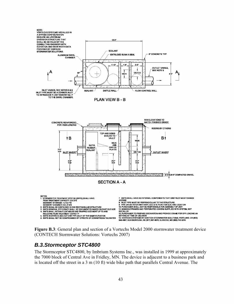
43
Figure B.3: General plan and section of a Vortechs Model 2000 stormwater treatment device (CONTECH Stormwater Solutions: Vortechs 2007)
B.3.Stormceptor STC4800 The Stormceptor STC4800, by Imbrium Systems Inc., was installed in 1999 at approximately the 7000 block of Central Ave in Fridley, MN. The device is adjacent to a business park and is located off the street in a 3 m (10 ft) wide bike path that parallels Central Avenue. The
44
device receives runoff from a large watershed, as evidenced by the fact that the structure is installed in-line within a 1.22 m (48 in) diameter storm drain pipe.
As can be seen in Figure B.4, the Stormceptor treatment device is a single manhole system, as opposed to the more commonly found multiple-chambered systems. An internal bypass is provided inside the structure such that flows with magnitude greater than the maximum treatment rate continue downstream without entering the treatment area. Stormwater is introduced at the upstream end of the treatment manhole and a swirling motion is induced by the ‘Stormceptor insert’, an inverted cone-like weir around a 0.25 m (10 in) diameter orifice plate, also as shown in Figure B.4. This insert was not included in the original installation in 1999. The Stormceptor that was evaluated for this research was retrofitted by Imbrium Systems, Inc. with this insert in the summer of 2006 to bring the installed unit up to current design standards. The Stormceptor insert is meant to function as both a diversion weir and a swirling motion inducer. Once water flows through the 0.25 m (10 in) orifice plate, it has entered the treatment chamber beneath the plastic/fiberglass floor separating the upper and lower chambers. Coarse, relatively heavy particles, such as sand, settle out of suspension to the invert of the manhole. Settling is assisted by the quiescent flow regime present in the treatment chamber, owing to the large diameter and depth of the treatment chamber. In order for the water inside the treatment chamber to escape the system and travel downstream, it must pass through a 0.6 m (24 in) diameter drop outlet pipe. The bottom of the outlet chute is approximately 1.5 m (5 ft) below the invert elevation of the storm drain pipe carrying effluent from the Stormceptor. The outlet pipe creates a trap and retention zone for light, buoyant materials, such as oil, grease and some organics that spans vertically from just beneath the fiberglass floor to the bottom of the drop outlet pipe. See Figure B.4 for a plan and section view of the Stormceptor STC4800, including the major features described above. Stormceptor utilizes a similar approach as that of other treatment devices, but provides for both coarse and buoyant material retention in a single structure, rather than multiple manholes. This installation of the STC4800 is 3 m (10 ft) in diameter and has a treatment chamber depth of 3.35 m (11 ft). Clearly a significant amount of storage for both grit and floatables has been provided in this installation. From grade level, the treatment chamber is accessed from a single manhole lid at the surface. After climbing a ladder down to the fiberglass floor separating the upper and lower chambers, a person(s) can be mechanically lowered through the drop outlet pipe to reach the sump. Maintenance of the Stormceptor STC4800 can be accomplished with a vacuum truck and a long suction hose; however, proper maintenance requires that a person enter the treatment sump to continually wash material toward the suction hose since the diameter of the chamber is so large, 3 m (10 ft), and the access point, i.e. the drop outlet pipe, is relatively small in comparison, 0.6 m (2 ft).
The hydrologic details of the watershed are unknown; according to the City of Fridley and Imbrium Systems, this particular unit was installed because it was the largest model on the market at the time. It is assumed the watershed encompasses a broad mix of residential, commercial, and industrial land uses. Thus, no rigorous sizing calculations were performed to determine the Stormceptor’s scale based on a maximum treatment rate or the maximum hydraulic rate. The unit does accommodate approximately 0.051 cms (1.8 cfs) before influent bypasses the Stormceptor insert weir; thus, 0.051 cms (1.8 cfs) is the maximum treatment rate as tested.

45
Figure B.4: General plan and section of a Stormceptor STC 4800 stormwater treatment device. In the section view of the depth to storm drain inlet, and the height of the treatment sump, the drawing indicates a varying depth and a minimum depth, respectively. (Stormceptor, 2007).
B.4. CDS Model PMSU20_15 The CDS Model PMSU20_15 was installed in the spring of 2006 in Minneapolis, MN, near the intersection of West Franklin Avenue and Ewing Avenue South, near Cedar Lake. It receives stormwater runoff from a 1.59 ha (3.92 ac), residential watershed.
This device is a single manhole system, with a deflective screening cylinder and floatables trap contained within the 1.52 m (5 ft) diameter structure. Stormwater is conveyed to the system by a 0.45 m (18 in) pipe in a direction normal to the manhole, but is introduced to the screening area tangentially through a fiberglass inlet chute. This chute also functions as an overflow weir to allow large flows to bypass settling treatment and continue downstream. Stormwater that enters the screening separation chamber has a swirling motion induced by the orientation of the inlet chute. As in the other devices, relatively heavier particulates
46
contained in the stormwater (sands, etc.) settle out of suspension in the settling chamber. Stormwater escapes the settling chamber by flowing through the 2400-micron sized openings in the 0.64 m (25 in) diameter stainless steel separation screen. Particles that cannot escape the screening cylinder settle to the bottom of treatment chamber sump where they can be removed with a vacuum truck. The sump is of larger diameter than the separation cylinder [1.52 m (60 in) sump vs. 0.64 m (25 in) separation chamber], which poses some difficulty when maintaining this unit. The suction hose from the vacuum truck has a limited range of mobility due to the smaller diameter separation cylinder directly above the sump. This necessitates that personnel enter the unit to manually move material to the center of the sump so it can be removed with the vacuum truck hose.
It should be noted that the removal mechanism is not straining; rather it is deflective separation since stormwater is flowing tangential to the screening surface. In this way, the action of the water is intended to prevent the screen from clogging with debris carried in stormwater. Upon exiting the separation chamber, water passes through a floatables trap before exiting the CDS by passing a baffle wall. The baffle wall only allows water to flow beneath it, whereby oils, some organics, or other buoyant material are retained. In this CDS unit, a distance of approximately 0.25 m (10 in) from the bottom of the baffle wall to the invert of the outlet pipe was provided for the retention of floatables.
Downstream of the device, the effluent from the CDS is conveyed a short distance by a 0.45 m (18 in) pipe, which empties into a wetland. There is a zero elevation gradient across the system from the inlet invert to the outlet invert. When combined with all of the head losses introduced by the CDS, the zero elevation gradient produces a backwater effect at the entrance to the CDS, which decreases the velocity of flow entering the device. The distance between the sump invert and the bottom of the slab separating the sump and floatables chamber is 0.6 m (24 in), as is the distance from the invert of the floatables chamber to the inverts of the inlet and outlet pipes. One access point is provided to the settling chamber, and one access point to the floatables trap. The structural features of the CDS PMSU20_15 can be found in the device plan and section illustrated in Figure B.5.
The CDS unit was designed to accommodate a maximum hydraulic flowrate equivalent to the 10-year event without flooding the street. According to calculations provided by CDS, the watershed has a runoff time of concentration of 45 minutes, corresponding to an intensity of 7.09 cm/hr (2.79 in/hr). The runoff coefficient was determined to be 0.45, producing a 10-year peak hydraulic flow of 0.14 cms (4.92 cfs) using the rational method. The calculated maximum capacity of the 0.45 m (18 in) pipes upstream and downstream was approximately 0.23 cms (8 cfs), which corresponds to approximately the 50-year event. Thus, the pipes around the CDS can easily handle its maximum hydraulic flowrate.
The CDS is an in-line system with an internal bypass provided, meaning the device will receive all flows traveling through the system, but treatment will not be provided above a certain water-quality event. According to calculations provided by CDS, the device is capable of removing 80.3% of the TSS contained in runoff on an annual basis while treating flows up to 0.024 cms (0.85 cfs). Flows above 0.024 cms (0.85 cfs) will bypass the system without treatment. Based on conversations with CDS technical personnel, this particular device was initially rated for 0.7 cfs but the weir height was raised a small amount to process

47
up to 0.024 cms (0.85 cfs) in order to reach the 80% annual TSS threshold. It was planned to evaluate the CDS both at approximately 0.020 cms (0.7 cfs) and 0.024 cms (0.85 cfs).
Figure B.5: Plan and section views of the CDS device evaluated at West Franklin & Ewing Avenue South in Minneapolis, MN (CDS Technologies, Inc., 2006).

48

49
Appendix C: Site Description, Preparation, and Field Test Procedure

50

51
C.1.Test Site Description and Preparation Four sites were chosen for assessment through field testing. Each site presented a unique device design to evaluate, a unique site layout, and preparatory hurdles to overcome to carry out successful field testing. Prior to the commencement of testing activities, each site required several general preparation procedures: 1) for real-time discharge measurement, a pre-calibrated circular weir and pressure transducer were installed. The pressure transducer measured water depths which, based on conduit geometry, was used to calculate flow areas and therefore discharge; 2) the BMP manholes were dewatered and accumulated solids were removed with the assistance of vacuum trucks provided by each city; 3) a piping system was customized for the delivery of hydrant water as influent test water, using each hydrant’s 10.2 cm (4 in) connection and a series of fittings, a 10.2 cm (4 in) gate valve, 15.2 cm (6 in) PVC pipe and/or 10.2 cm (4 in) flexible fire hose donated by the City of Fridley Public Works and Fire Departments, and hydrant fittings to allow connection to all types of hydrant threadings encountered in the Twin Cities. A gate valve was necessary to control water output from the hydrant since they are not designed to be only partially open—either fully open or closed; 4) sand was pre-sieved into three discreet size ranges for use in each simulated runoff event, as described in Appendix A; and 5) inflatable plugs were secured either from each city or from a rental vendor to seal off storm drain upstream of the treatment system to eliminate nuisance flows in the system. Additionally, an effluent discharge permit was granted by the Minnesota Pollution Control Agency to cover field testing activities at the four sites. Permits for use of fire hydrants were secured from the appropriate agency in each community in which testing was completed.
The specific site features, preparatory steps, and/or challenges will be discussed in chronological order of testing, beginning with the V2B1 model 4, followed by the Vortechs System 2000, the Stormceptor STC4800, and finally the CDS PMSU20_15. The laboratory tests are described in Carlson et al. (2006) and Mohseni and Fyten (2007).
C.2.V2B1 Model 4 The V2B1 Model 4, by Environment21, was installed in 2005 in New Brighton, Minnesota, at the intersection of Rice Creek Road and Long Lake Road, as shown in Figure C.1. Long Lake ultimately receives the runoff from the watershed and thus the effluent from the V2B1 device. It was necessary to utilize both the northern and southern portions of Rice Creek Road for equipment storage and system access at this intersection since both sides of the street contained structures of interest, as Figure C.1 illustrates.
Several trips to the site were undertaken as mobilization efforts, including those for anchoring a 0.38 m (15 in) circular weir and anchoring a metal clip used to secure the pressure transducer probe in place so it would remain stable while effluent discharge passed over it. The 5.1 cm (2 in) tall circular weir was installed at the end of the 0.38 m (15 in) pipe as illustrated in Figure C.2 to ensure that the discharge would flow under free outfall
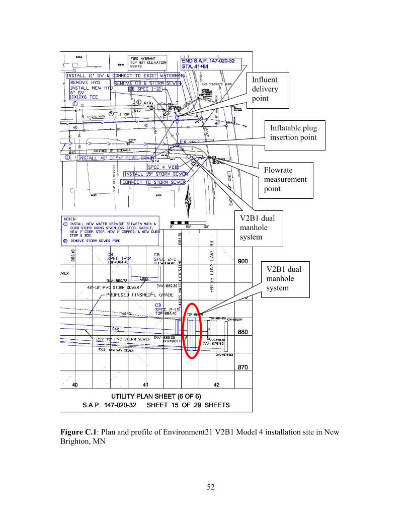
52
Figure C.1: Plan and profile of Environment21 V2B1 Model 4 installation site in New Brighton, MN
V2B1 dual manhole system
Influent delivery point
Flowrate measurement point
Inflatable plug insertion point
V2B1 dual manhole system

53
Figure C.2: Pre-calibrated 0.38 m (15 in) circular weir installed downstream of the V2B1. Pressure transducer and transducer anchoring not shown. This weir location provided free outfall conditions at all flowrates due to the PVC pipe’s favorable elevation vs. the existing 0.9 m (36 in) storm drain pipe it discharged into. conditions, which corresponded to the calibration conditions. The transducer probe clip was installed approximately 0.6 m (2 ft) upstream of the weir. Both the transducer clip and weir anchors were set by tapping into the 0.38 m (15 in) PVC pipe. It was intended for the transducer probe to be inserted into the clip upon arrival at the site each day and removed when leaving the site in the afternoon so as to prevent damage from high flow storm events, corrosion, etc.
Before any testing activities could begin, the treatment manholes had to be clean. In the case of the V2B1 in New Brighton, a significant amount of material was present inside the swirl chamber despite being installed only a few months prior. This in part was due to the fact that a portion of the watershed was an active construction site that produced a higher sediment load than would normally be expected. The initial cleanout task was greatly assisted by the City of New Brighton’s vacuum truck and crew, who were able to dewater the device and remove the majority of the solids (about 1.7 m3 [2.2 yd3]) relatively quickly. One problem encountered by the city maintenance crew was in removing all the material directly beneath the 0.6 m (24 in) PVC standpipe structure inside the swirl chamber. This standpipe (see Figure B.1) blocked complete access to the treatment chamber invert by the vacuum truck suction hose. As a result, approximately 0.4 m3 (0.5 yd3) of coarse material was not vacuumed out of the swirl chamber by the vacuum truck. Following the assistance of the city crew and vacuum truck, the remaining fine-tune cleaning was accomplished with shovels, buckets, and a small wet-dry vacuum. The assumption was that City vacuum truck assistance
Pressure transducer location (not shown)
0.38 m circular weir
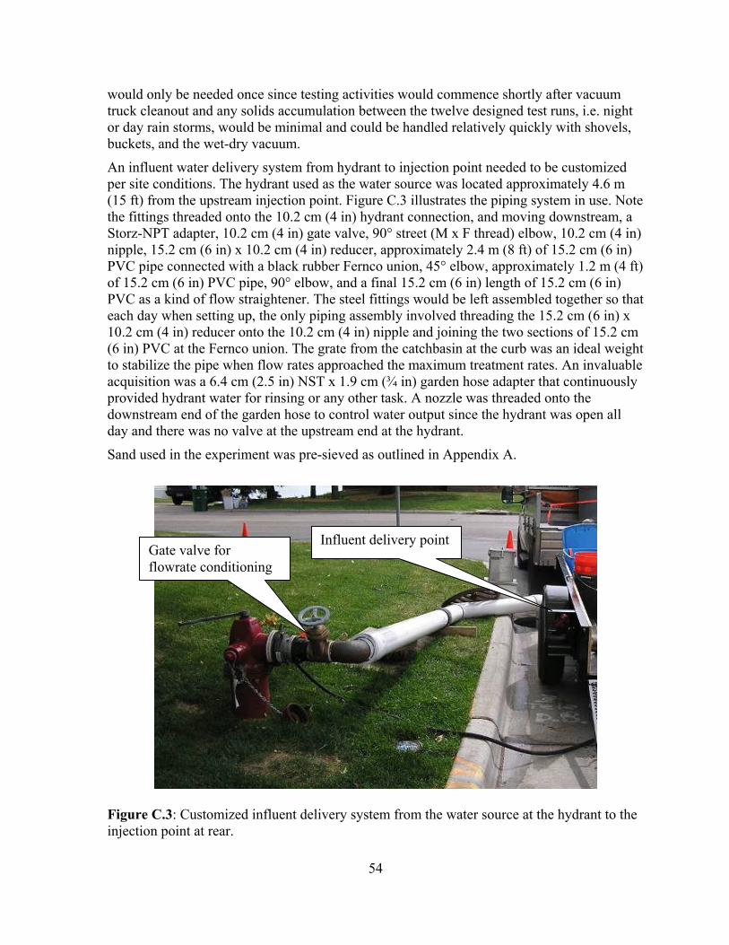
54
would only be needed once since testing activities would commence shortly after vacuum truck cleanout and any solids accumulation between the twelve designed test runs, i.e. night or day rain storms, would be minimal and could be handled relatively quickly with shovels, buckets, and the wet-dry vacuum.
An influent water delivery system from hydrant to injection point needed to be customized per site conditions. The hydrant used as the water source was located approximately 4.6 m (15 ft) from the upstream injection point. Figure C.3 illustrates the piping system in use. Note the fittings threaded onto the 10.2 cm (4 in) hydrant connection, and moving downstream, a Storz-NPT adapter, 10.2 cm (4 in) gate valve, 90° street (M x F thread) elbow, 10.2 cm (4 in) nipple, 15.2 cm (6 in) x 10.2 cm (4 in) reducer, approximately 2.4 m (8 ft) of 15.2 cm (6 in) PVC pipe connected with a black rubber Fernco union, 45° elbow, approximately 1.2 m (4 ft) of 15.2 cm (6 in) PVC pipe, 90° elbow, and a final 15.2 cm (6 in) length of 15.2 cm (6 in) PVC as a kind of flow straightener. The steel fittings would be left assembled together so that each day when setting up, the only piping assembly involved threading the 15.2 cm (6 in) x 10.2 cm (4 in) reducer onto the 10.2 cm (4 in) nipple and joining the two sections of 15.2 cm (6 in) PVC at the Fernco union. The grate from the catchbasin at the curb was an ideal weight to stabilize the pipe when flow rates approached the maximum treatment rates. An invaluable acquisition was a 6.4 cm (2.5 in) NST x 1.9 cm (¾ in) garden hose adapter that continuously provided hydrant water for rinsing or any other task. A nozzle was threaded onto the downstream end of the garden hose to control water output since the hydrant was open all day and there was no valve at the upstream end at the hydrant.
Sand used in the experiment was pre-sieved as outlined in Appendix A.
Figure C.3: Customized influent delivery system from the water source at the hydrant to the injection point at rear.
Gate valve for flowrate conditioning
Influent delivery point
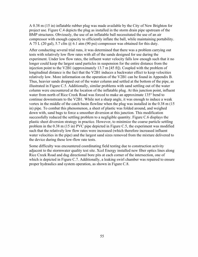
55
A 0.38 m (15 in) inflatable rubber plug was made available by the City of New Brighton for project use. Figure C.4 depicts the plug as installed in the storm drain pipe upstream of the BMP structures. Obviously, the use of an inflatable ball necessitated the use of an air compressor with enough capacity to efficiently inflate the ball, while maintaining portability. A 75 L (20 gal), 5.7 cfm @ 6.1 atm (90 psi) compressor was obtained for this duty.
After conducting several trial runs, it was determined that there was a problem carrying out tests with relatively low flow rates with all of the sands designed for use during the experiment. Under low flow rates, the influent water velocity falls low enough such that it no longer could keep the largest sand particles in suspension for the entire distance from the injection point to the V2B1 (approximately 13.7 m [45 ft]). Coupled with the problem of longitudinal distance is the fact that the V2B1 induces a backwater effect to keep velocities relatively low. More information on the operation of the V2B1 can be found in Appendix B. Thus, heavier sands dropped out of the water column and settled at the bottom of the pipe, as illustrated in Figure C.5. Additionally, similar problems with sand settling out of the water column were encountered at the location of the inflatable plug. At this junction point, influent water from north of Rice Creek Road was forced to make an approximate 135° bend to continue downstream to the V2B1. While not a sharp angle, it was enough to induce a weak vortex in the middle of the catch basin flowline when the plug was installed in the 0.38 m (15 in) pipe. To combat this phenomenon, a sheet of plastic was folded around, and weighed down with, sand bags to force a smoother diversion at this junction. This modification successfully reduced the settling problem to a negligible quantity. Figure C.6 displays the plastic sheet diversion strategy in practice. However, to minimize the coarse particle settling problem in the 0.38 m (15 in) PVC pipe depicted in Figure C.5, the experiment was modified such that the relatively low flow rates were increased (which therefore increased influent water velocities in the pipe) and the largest sand sizes removed from the mixture delivered to the device during these low-flow rate tests.
Some difficulty was encountered coordinating field testing due to construction activity adjacent to the stormwater quality test site. Xcel Energy installed new fiber optics lines along Rice Creek Road and dug directional bore pits at each corner of the intersection, one of which is depicted in Figure C.7. Additionally, a leaking swirl chamber was repaired to ensure proper hydraulics and system operation, as shown in Figure C.8.

56
Figure C.4: 0.45 m (18 in) diameter inflatable plug loaned by the City of New Brighton Public Works for use where indicated in Figure C.3.
Figure C.5: Illustration of particle settling phenomenon inside the swirl chamber’s influent delivery pipe. It is clear that a sandbar has formed which is believed to contribute to further settling by reducing the vertical settling distance in this pipe.
0.38 m PVC inlet pipe carrying influent water & sediment into V2B1
Sandbar formation typical of large particle settling problems
Inflatable plug to seal off upstream reaches
0.38 m PVC pipe leading to V2B1

57
Figure C.6: Use of a plastic sheet weighed down with sandbags to smoothly turn water downstream toward the V2B1 (water moving right to left) and therefore eliminate coarse sand particle settling in front of the inflatable plug due to weak vortices.
Figure C.7: Contention of field testing with construction activities.
Diversion straightening via plastic sheet & sand bags
V2B1 location
58
Figure C.8: (Left) Water was initially able to flow between treatment manholes through an approximate 1.3 cm ( ½ in) gap between the PVC pipe and concrete manhole wall. (Right) The leaking gap was patched with Vulcum polyurethane to ensure proper system hydraulics.
C.3. Vortechs Model 2000 The Vortechs Model 2000, by Stormwater360, Inc., was installed in 2005 in St. Louis Park, MN at the southeast corner of a residential loft redevelopment site near the intersection of 41st Street West and Vernon Avenue, which is a frontage road along Highway 100. Figure C.9 below depicts the site drainage plan.
Similarly to the V2B1 tested previous to the Vortechs System, some trips to the site were necessary for general reconnaissance and setup. As shown in Figure C.10, a 0.3 m (12 in) circular weir with a height of 4.1 cm (1.6 in) and metal clip for the pressure transducer were installed downstream of the Vortechs System unit at a spot with more than enough elevation gradient across the manhole flowline to ensure free outfall conditions to provide appropriate weir flow conditions. This location was approximately 28.3 m (93 ft) downstream of the Vortechs System. It was deemed likely that a weir installed upstream of this location would be inhibited by tailwater effects which would produce inaccurate discharge data. The anchoring for the circular weir required a hammer drill to bore the holes to set anchors into the 0.3 m (12 in) pipe. The relatively small size of the pipe necessitated a compressed air-powered hammer drill with a smaller size.
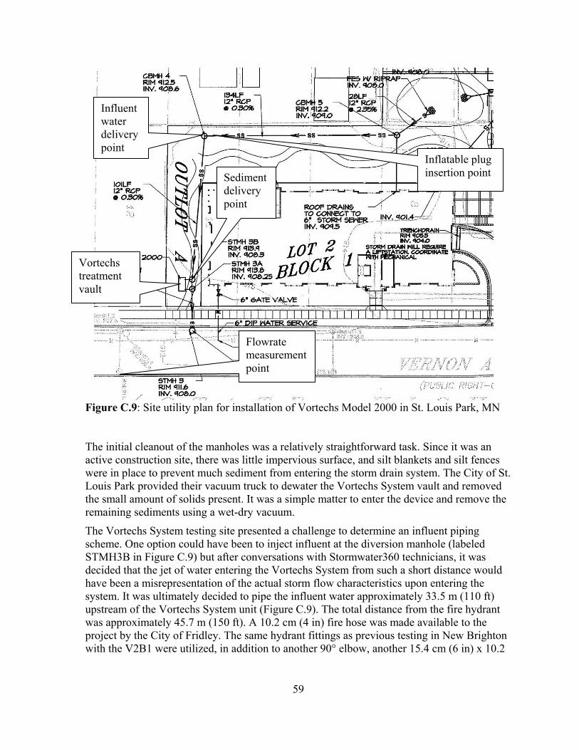
59
Figure C.9: Site utility plan for installation of Vortechs Model 2000 in St. Louis Park, MN The initial cleanout of the manholes was a relatively straightforward task. Since it was an active construction site, there was little impervious surface, and silt blankets and silt fences were in place to prevent much sediment from entering the storm drain system. The City of St. Louis Park provided their vacuum truck to dewater the Vortechs System vault and removed the small amount of solids present. It was a simple matter to enter the device and remove the remaining sediments using a wet-dry vacuum.
The Vortechs System testing site presented a challenge to determine an influent piping scheme. One option could have been to inject influent at the diversion manhole (labeled STMH3B in Figure C.9) but after conversations with Stormwater360 technicians, it was decided that the jet of water entering the Vortechs System from such a short distance would have been a misrepresentation of the actual storm flow characteristics upon entering the system. It was ultimately decided to pipe the influent water approximately 33.5 m (110 ft) upstream of the Vortechs System unit (Figure C.9). The total distance from the fire hydrant was approximately 45.7 m (150 ft). A 10.2 cm (4 in) fire hose was made available to the project by the City of Fridley. The same hydrant fittings as previous testing in New Brighton with the V2B1 were utilized, in addition to another 90° elbow, another 15.4 cm (6 in) x 10.2
Vortechs treatment vault
Influent water delivery point
Flowrate measurement point
Inflatable plug insertion point Sediment
delivery point
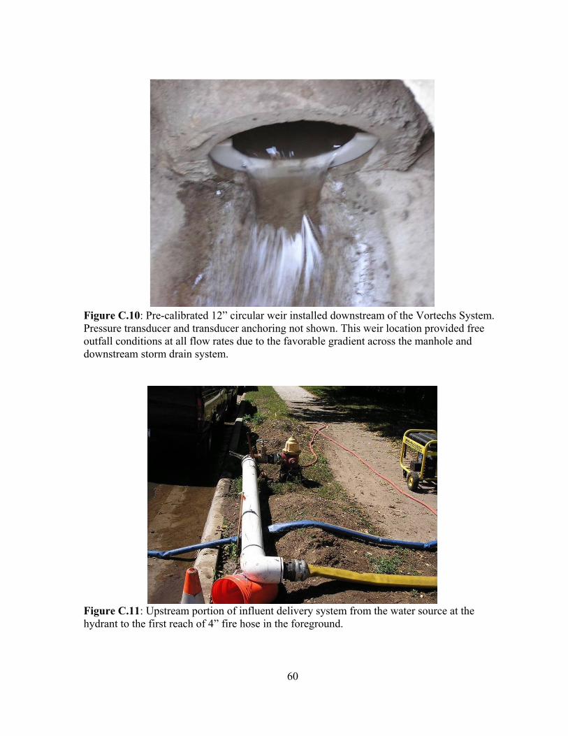
60
Figure C.10: Pre-calibrated 12” circular weir installed downstream of the Vortechs System. Pressure transducer and transducer anchoring not shown. This weir location provided free outfall conditions at all flow rates due to the favorable gradient across the manhole and downstream storm drain system.
Figure C.11: Upstream portion of influent delivery system from the water source at the hydrant to the first reach of 4” fire hose in the foreground.
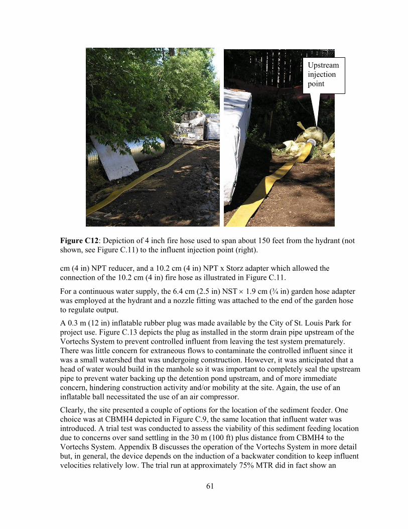
61
Figure C12: Depiction of 4 inch fire hose used to span about 150 feet from the hydrant (not shown, see Figure C.11) to the influent injection point (right). cm (4 in) NPT reducer, and a 10.2 cm (4 in) NPT x Storz adapter which allowed the connection of the 10.2 cm (4 in) fire hose as illustrated in Figure C.11.
For a continuous water supply, the 6.4 cm (2.5 in) NST × 1.9 cm (¾ in) garden hose adapter was employed at the hydrant and a nozzle fitting was attached to the end of the garden hose to regulate output.
A 0.3 m (12 in) inflatable rubber plug was made available by the City of St. Louis Park for project use. Figure C.13 depicts the plug as installed in the storm drain pipe upstream of the Vortechs System to prevent controlled influent from leaving the test system prematurely. There was little concern for extraneous flows to contaminate the controlled influent since it was a small watershed that was undergoing construction. However, it was anticipated that a head of water would build in the manhole so it was important to completely seal the upstream pipe to prevent water backing up the detention pond upstream, and of more immediate concern, hindering construction activity and/or mobility at the site. Again, the use of an inflatable ball necessitated the use of an air compressor.
Clearly, the site presented a couple of options for the location of the sediment feeder. One choice was at CBMH4 depicted in Figure C.9, the same location that influent water was introduced. A trial test was conducted to assess the viability of this sediment feeding location due to concerns over sand settling in the 30 m (100 ft) plus distance from CBMH4 to the Vortechs System. Appendix B discusses the operation of the Vortechs System in more detail but, in general, the device depends on the induction of a backwater condition to keep influent velocities relatively low. The trial run at approximately 75% MTR did in fact show an
Upstream injection point

62
extreme settling problem, with very little sand reaching the device. Much of the sand was concentrated at the injection manhole, with the remainder settled out someplace along the 30 m (100 ft) reach of pipe, examples of which can be found in Figure C.14. This phenomenon was especially problematic since it occurred at a relatively high flowrate (approximately 75% MTR), so it would be expected to occur to a greater extent with lower flowrates. As a result, the decision was made to keep the water injection point at the same location, but move the sediment feeder to STMH3B illustrated in Figure C.9. The sediment feeding location was set at approximately 1.8 m (6 ft) upstream of the Vortechs System, and upon inspection during testing, STMH3B provided a good mixing zone due to the presence of the weir inside the manhole diverting flow to the Vortechs System. Figure C.15 illustrates the sediment feeder setup at STMH3B.
Figure C.13: 12” diameter inflatable plug loaned by the City of St. Louis Park Public Works for use at CBMH4 as shown in Figure C.12. The Vortechs System had to undergo some patchwork in a similar way to the V2B1. The swirl chamber inside the Vortechs System is a stainless steel cylinder inside a rectangular vault, with a sealant at the bottom to prevent underflow scouring settled material downstream to the floatables trap. However, a portion of the circumference at the base of the stainless steel cylinder was missing any kind of sealant. When pumping out the settling chamber, water was observed flowing in from the floatables trap, carrying sediment with it. To minimize potential errors due to this type of problem, the section was sealed with Vulcum polyurethane. Figure C.16 depicts the section requiring patching, which was approximately 25% of the circumference.
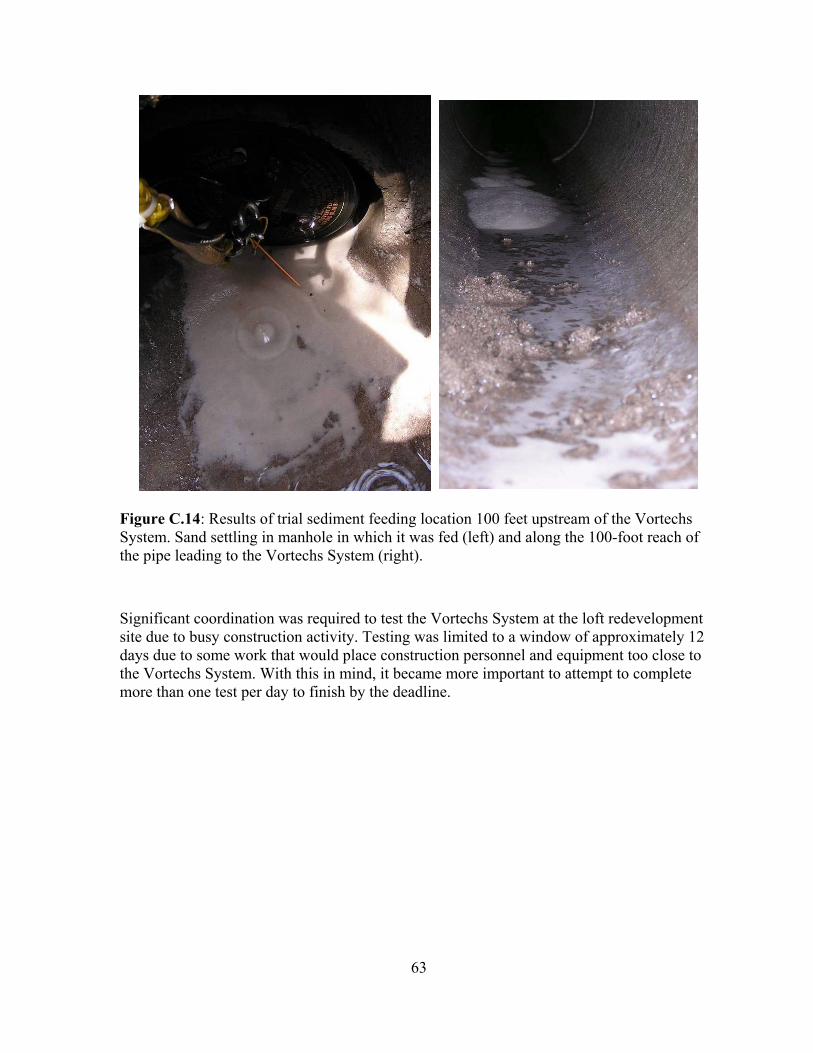
63
Figure C.14: Results of trial sediment feeding location 100 feet upstream of the Vortechs System. Sand settling in manhole in which it was fed (left) and along the 100-foot reach of the pipe leading to the Vortechs System (right).
Significant coordination was required to test the Vortechs System at the loft redevelopment site due to busy construction activity. Testing was limited to a window of approximately 12 days due to some work that would place construction personnel and equipment too close to the Vortechs System. With this in mind, it became more important to attempt to complete more than one test per day to finish by the deadline.
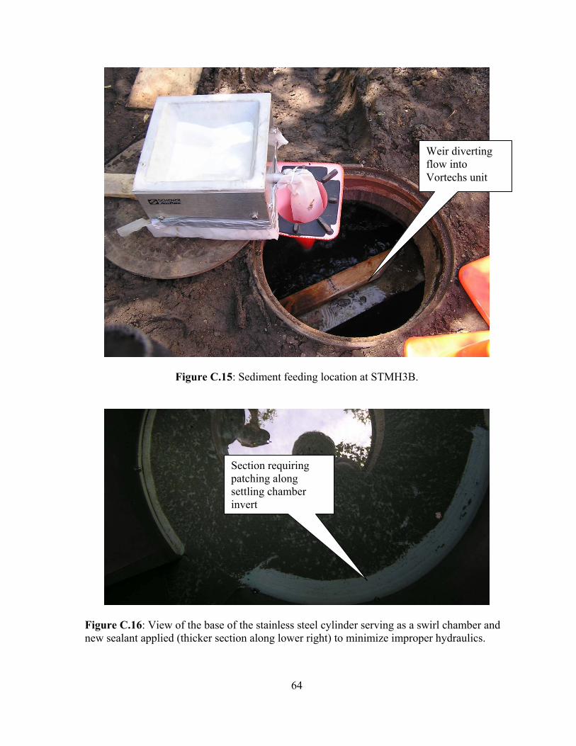
64
Figure C.15: Sediment feeding location at STMH3B.
Figure C.16: View of the base of the stainless steel cylinder serving as a swirl chamber and new sealant applied (thicker section along lower right) to minimize improper hydraulics.
Weir diverting flow into Vortechs unit
Section requiring patching along settling chamber invert

65
C.4.Stormceptor STC4800 The Stormceptor STC4800, by Imbrium Systems Inc., was installed in 1999 at approximately the 7000 block of Central Ave in Fridley, MN, and retrofitted by Imbrium in the summer of 2006 before testing commenced. The device is adjacent to a business park and is located off the street in a 3m (10 ft) wide bike path that parallels Central Avenue. A plan and profile for the storm drain in which the Stormceptor was installed is included as Figure C.17. The proximity to the industrial park afforded plenty of space for the truck and trailer rig to park and plenty of storage for equipment necessary for testing. The Stormceptor receives water from a large watershed, as evidenced by the fact that the device is located in-line with a 1.2 m (48 in) RCP. From an experiment design standpoint, the Stormceptor presented some difficulty due to its sheer size, especially in comparison to the two previously evaluated devices. Appendix B discusses Stormceptor operation in detail but the treatment chamber is 3 m (10 ft) diameter and a depth of 3.4 m (11 ft). The top of the treatment chamber is approximately 3.7 m (12 ft) below the ground surface, which complicated the experiment, i.e. access to the treatment chamber was through a 0.6 m (2 ft) diameter and approximate 1.5 m (5 ft) tall cylindrical shaft.
Some pilot testing was conducted on the Stormceptor in the fall of 2005 to determine the type of equipment necessary to purchase and/or design before full time field testing commenced in the spring of 2006. As a part of the pilot testing, a 48-inch diameter circular weir with an approximate height of 6.4 cm (2.5 in) was installed at the manhole immediately downstream of the Stormceptor for flowrate measurement with a pressure transducer. However, a backwater condition just downstream of the weir prevented free outfall conditions with that particular weir height. As a result, during summer 2006 testing, a new and taller weir height of 17.5 cm (6.9 in) was installed to prevent a backwater effect. To be more confident of free outfall conditions, the weir was aerated to ensure the existence of an air bubble below the lower nap as water passed over the crest. Figure C.18 illustrates the aerated weir and transducer cable in place inside the 1.2 m (48 in) pipe.
The City of Fridley offered the use of their vacuum truck and maintenance crew to help with the initial cleanout of the treatment chamber. Normally, the device is maintained yearly, in the fall, so there was material accumulation from fall, winter, and spring months to remove. The device was first dewatered, which required two tank loads of the vacuum truck, and then personnel were mechanically lowered into the sump area to operate the suction hose while rinsing the walls and floor. Once the majority of the solids were removed with the City’s assistance, the remaining fine-tune cleaning was accomplished with a series of rinsing and wet-dry vacuuming iterations. An inconvenience with the Stormceptor site involved mortar along the treatment chamber invert chipping off each time the area was cleaned. Thus, more time was spent vacuuming these areas until it was determined that sand-sized particles had finished shearing off the mortar.
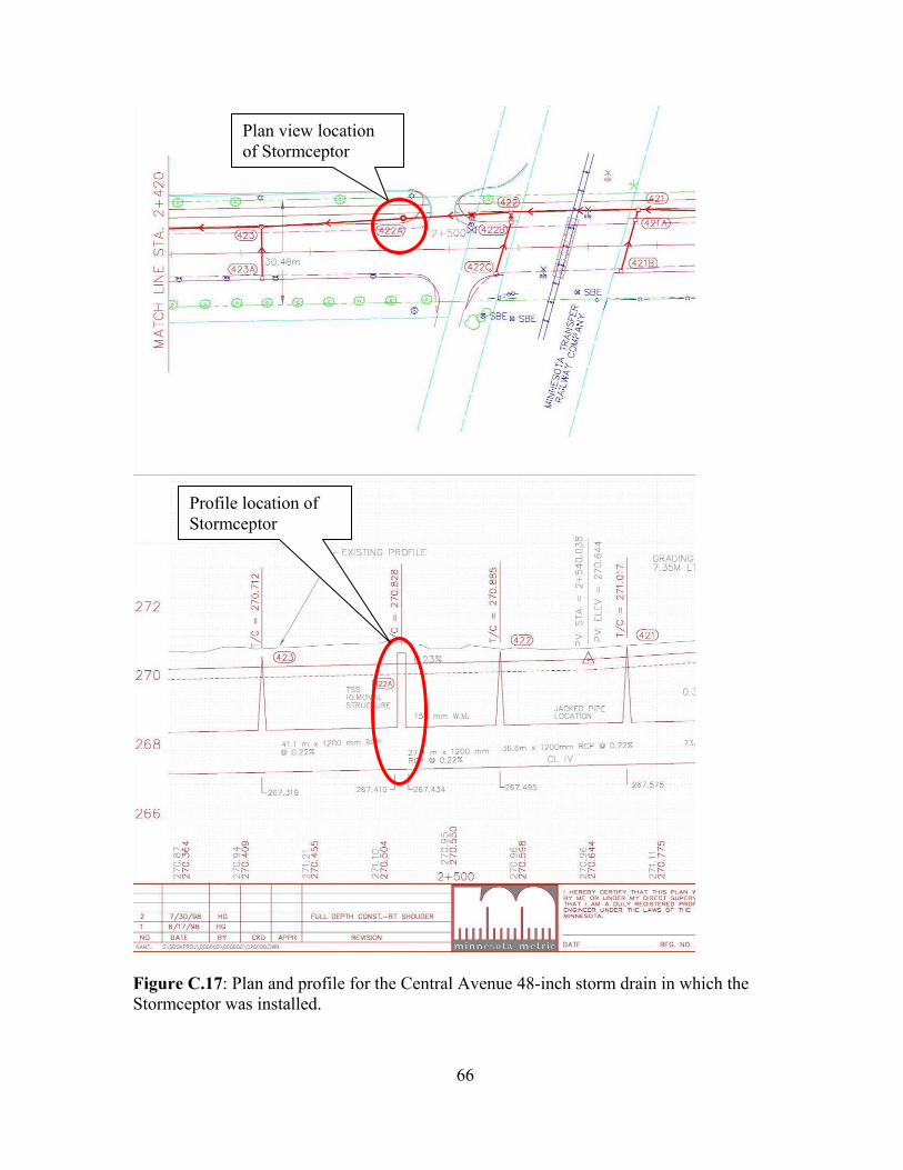
66
Figure C.17: Plan and profile for the Central Avenue 48-inch storm drain in which the Stormceptor was installed.
Plan view location of Stormceptor
Profile location of Stormceptor
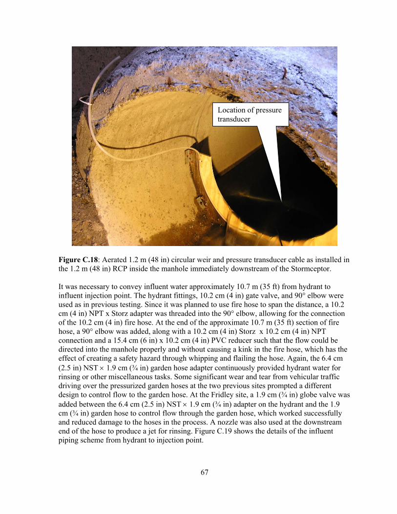
67
Figure C.18: Aerated 1.2 m (48 in) circular weir and pressure transducer cable as installed in the 1.2 m (48 in) RCP inside the manhole immediately downstream of the Stormceptor.
It was necessary to convey influent water approximately 10.7 m (35 ft) from hydrant to influent injection point. The hydrant fittings, 10.2 cm (4 in) gate valve, and 90° elbow were used as in previous testing. Since it was planned to use fire hose to span the distance, a 10.2 cm (4 in) NPT x Storz adapter was threaded into the 90° elbow, allowing for the connection of the 10.2 cm (4 in) fire hose. At the end of the approximate 10.7 m (35 ft) section of fire hose, a 90° elbow was added, along with a 10.2 cm (4 in) Storz x 10.2 cm (4 in) NPT connection and a 15.4 cm (6 in) x 10.2 cm (4 in) PVC reducer such that the flow could be directed into the manhole properly and without causing a kink in the fire hose, which has the effect of creating a safety hazard through whipping and flailing the hose. Again, the 6.4 cm (2.5 in) NST × 1.9 cm (¾ in) garden hose adapter continuously provided hydrant water for rinsing or other miscellaneous tasks. Some significant wear and tear from vehicular traffic driving over the pressurized garden hoses at the two previous sites prompted a different design to control flow to the garden hose. At the Fridley site, a 1.9 cm (¾ in) globe valve was added between the 6.4 cm (2.5 in) NST × 1.9 cm (¾ in) adapter on the hydrant and the 1.9 cm (¾ in) garden hose to control flow through the garden hose, which worked successfully and reduced damage to the hoses in the process. A nozzle was also used at the downstream end of the hose to produce a jet for rinsing. Figure C.19 shows the details of the influent piping scheme from hydrant to injection point.
Location of pressure transducer

68
Figure C.19: Influent piping configuration, making use of the same hydrant fittings as at previous testing sites and a reach of fire hose to cover the ~10 m (35 ft) from hydrant to influent delivery point. Determining a method for sealing off upstream reaches of the 1.2 m (48 in) storm drain proved problematic. The plugging of the upstream pipe was particularly important due to a couple of factors. First, due to the size of the watershed, and therefore the potential for runoff and groundwater to be captured and conveyed by the storm drain system, there was always a base flow of around 0.95 L/s (15 gpm) to 1.9 L/s (30 gpm) running through the pipe that needed to be blocked upstream of the feeding point. Second, the storm drain system was constructed with a slope of 0.3%, so the plug allowed for a head of water to build up and push water downstream to the Stormceptor without escaping temporarily from the upstream end. During pilot testing in the fall of 2005, the standard style of 1.2 m (48 in) diameter test ball was considered for feasibility of use during testing. It was very large (when deflated, approximately 0.9 m (3 ft) diameter and 1.5 m (5 ft) long), bulky, weighed around 90 kg (200 lb), and was extremely difficult to maneuver into and out of the manhole providing access to the pipe. Another downside was the significant rental cost of the plug. One alternative involved designing an in-house plug using metal bracing and plywood sheeting. It offered some ease of placement over the standard inflatable test ball, but setup time was a concern, as was the kind of seal that could be expected from the customized plug, as well as the height of water the plug could withstand behind it. Alternative two made use of a special type of inflatable plug, called a ‘pillow style’ test ball. It is unique in that it has much less rigidity in its structure than the standard style and has the ability to fold up like a sheet into a rectangular shape of around 0.45 m (18 in) x 0.45 m (18 in). Additionally, it is much lighter (about 13 kg [30 lb])) and simple to maneuver through a manhole lid. The downside to this added convenience was the rental cost to bear. In the end, however, alternative two (pillow-style test ball) was selected due to more certainty of performance as well as the simplicity and time savings involved with its setup. This style of test ball could be inflated with the 75.7 L (20 gal), 5.7 cfm air compressor used at the V2B1 site, but required several tanks of air. As
Influent delivery point

69
a result, the compressor was plugged into the 5 kW generator while inflating the plug to allow it to refill whenever necessary.
Due to concerns similar to those faced at other sites over sediment deposition in the pipe upstream of the Stormceptor, the sediment feeding location needed to be selected carefully. It was determined that little or no coarse sediment would likely reach the Stormceptor if the sediment was introduced at the same spot as influent water, i.e. approximately 23 m (75 ft) upstream in the pipe. Since the pipe was so large and flat, the range of flow rates of interest to the field testing would produce a small water depth, resulting in a shallow settling distance and the flow would travel relatively slowly down the pipe, a combination that would be problematic. Therefore, it was decided to deliver sediment closer to the Stormceptor. A system was devised that would introduce sediment approximately 1.8 m (6 ft) upstream of the device, shown in Figures C.20 and C.21. Sand was delivered by the sediment feeder at the ground surface into a vertically mounted 5.1 cm (2 in) diameter PVC pipe. To prevent clogging at the 90° elbow at the bottom, a wye fitting was attached to the top of the PVC to allow the garden hose to be secured and, while it was being augured, continually wash the sand through the PVC. The water-sand slurry was delivered along the centerline of the 1.2 m (48 in) pipe with the assistance of a 90° elbow, where it underwent mixing through the shallow water column before flowing into the Stormceptor.
Figure C.20: Illustration of sediment delivery system to prevent sediment deposition in the upstream pipe. In the photo at left, the sediment feeder augured into a 10.2 cm (2 in) diameter PVC pipe where it was met by wash water from a garden hose to prevent clogging at the elbow at the bottom of the pipe depicted at right.
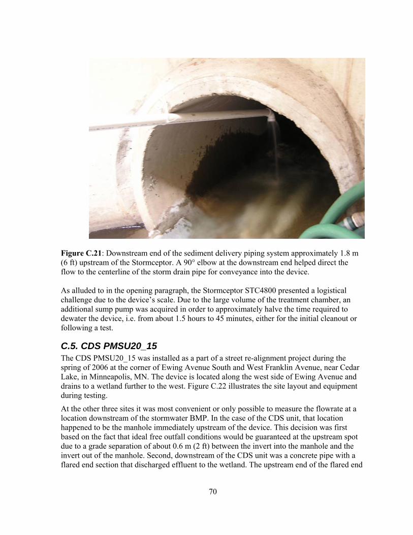
70
Figure C.21: Downstream end of the sediment delivery piping system approximately 1.8 m (6 ft) upstream of the Stormceptor. A 90° elbow at the downstream end helped direct the flow to the centerline of the storm drain pipe for conveyance into the device. As alluded to in the opening paragraph, the Stormceptor STC4800 presented a logistical challenge due to the device’s scale. Due to the large volume of the treatment chamber, an additional sump pump was acquired in order to approximately halve the time required to dewater the device, i.e. from about 1.5 hours to 45 minutes, either for the initial cleanout or following a test.
C.5. CDS PMSU20_15 The CDS PMSU20_15 was installed as a part of a street re-alignment project during the spring of 2006 at the corner of Ewing Avenue South and West Franklin Avenue, near Cedar Lake, in Minneapolis, MN. The device is located along the west side of Ewing Avenue and drains to a wetland further to the west. Figure C.22 illustrates the site layout and equipment during testing.
At the other three sites it was most convenient or only possible to measure the flowrate at a location downstream of the stormwater BMP. In the case of the CDS unit, that location happened to be the manhole immediately upstream of the device. This decision was first based on the fact that ideal free outfall conditions would be guaranteed at the upstream spot due to a grade separation of about 0.6 m (2 ft) between the invert into the manhole and the invert out of the manhole. Second, downstream of the CDS unit was a concrete pipe with a flared end section that discharged effluent to the wetland. The upstream end of the flared end
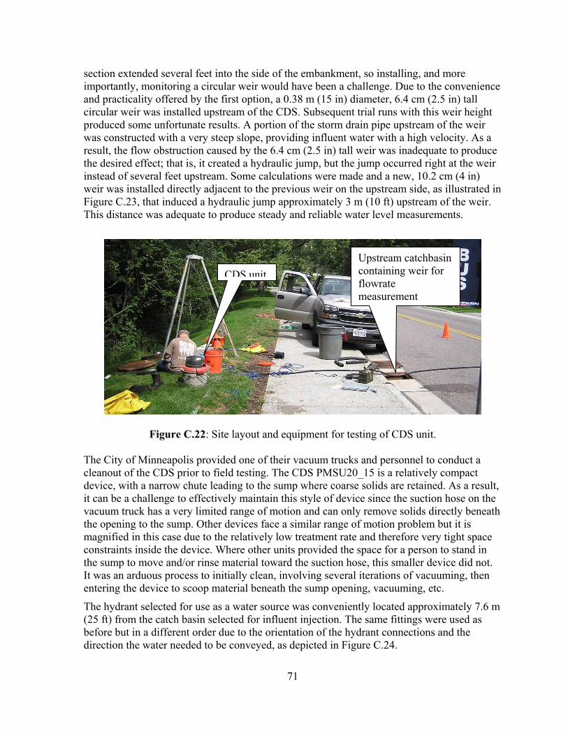
71
section extended several feet into the side of the embankment, so installing, and more importantly, monitoring a circular weir would have been a challenge. Due to the convenience and practicality offered by the first option, a 0.38 m (15 in) diameter, 6.4 cm (2.5 in) tall circular weir was installed upstream of the CDS. Subsequent trial runs with this weir height produced some unfortunate results. A portion of the storm drain pipe upstream of the weir was constructed with a very steep slope, providing influent water with a high velocity. As a result, the flow obstruction caused by the 6.4 cm (2.5 in) tall weir was inadequate to produce the desired effect; that is, it created a hydraulic jump, but the jump occurred right at the weir instead of several feet upstream. Some calculations were made and a new, 10.2 cm (4 in) weir was installed directly adjacent to the previous weir on the upstream side, as illustrated in Figure C.23, that induced a hydraulic jump approximately 3 m (10 ft) upstream of the weir. This distance was adequate to produce steady and reliable water level measurements.
Figure C.22: Site layout and equipment for testing of CDS unit. The City of Minneapolis provided one of their vacuum trucks and personnel to conduct a cleanout of the CDS prior to field testing. The CDS PMSU20_15 is a relatively compact device, with a narrow chute leading to the sump where coarse solids are retained. As a result, it can be a challenge to effectively maintain this style of device since the suction hose on the vacuum truck has a very limited range of motion and can only remove solids directly beneath the opening to the sump. Other devices face a similar range of motion problem but it is magnified in this case due to the relatively low treatment rate and therefore very tight space constraints inside the device. Where other units provided the space for a person to stand in the sump to move and/or rinse material toward the suction hose, this smaller device did not. It was an arduous process to initially clean, involving several iterations of vacuuming, then entering the device to scoop material beneath the sump opening, vacuuming, etc.
The hydrant selected for use as a water source was conveniently located approximately 7.6 m (25 ft) from the catch basin selected for influent injection. The same fittings were used as before but in a different order due to the orientation of the hydrant connections and the direction the water needed to be conveyed, as depicted in Figure C.24.
CDS unitUpstream catchbasin containing weir for flowrate measurement

72
Figure C.23: Initially installed weir and final weir directly behind it (upstream side), for flow rate measurement. The pressure transducer probe and clip anchoring upstream of the weir are not shown. It was determined that no inflatable test balls were necessary to acquire for field testing the CDS. This particular facility treats a small residential watershed, so unless a resident washed his or her car, or some similar activity, there were no base flows present in the system to seal off. Additionally, the pipe directly upstream of the CDS was installed on a steep gradient, which negated any tendency for influent water to be temporarily stored upstream. Prior to testing, when hydrant water was run through the system to simulate real conditions, no water was observed to be stored upstream. Thus, a plug was deemed unnecessary.
It was originally intended for sediment to be added to the system at the catchbasin immediately upstream of the CDS, approximately 4.6 m (15 ft) upstream. Unfortunately when this location for sediment feeding was evaluated in two trial runs, significant sand settling problems presented themselves in the 0.38 m (15 in) pipe upstream of the CDS. The design of the CDS called for an internal overflow bypass chute structure that induces a backwater effect on the storm drain system that slows flow velocities to a low level. In addition, a sudden expansion as water is introduced to the overflow bypass chute compounds the phenomenon of slowing velocities. See Appendix B for a more detailed description of the operation of the CDS device. As a result, it became necessary to design a sediment delivery
Initially installed 10.2 cm diameter weir
Subsequent 15.4 cm diameter weir
Location of pressure transducer

73
Figure C.24: Influent piping system from hydrant to catch basin for CDS testing. system similar to that employed at the Stormceptor site in Fridley. PVC pipe and fittings were assembled at the surface, above the manhole ring providing access to the CDS. Water from a garden hose would again be washed into the PVC pipe to prevent clogging of dry sand, resulting in a slurry mixture ultimately introduced to the CDS. The first attempted delivery point was at the soffit of the upstream pipe, approximately 0.6 m (2 ft) upstream of the expansion. This feeding location, too, resulted in settling, this time in the overflow chute at the expansion. Next, the delivery point was moved downstream such that sand was delivered just at the expansion, but to similar settling problems in the chute. Finally, the delivery point was moved once more downstream, approximately 2/3 of the way longitudinally down the chute. This location was able to completely deliver the slurry to the CDS without upstream sand settlement. Figure C.25 depicts the final sediment delivery setup.
The CDS required some work to repair a leaking seam in the treatment cylinder between the stainless steel cylindrical screen and the fiberglass cylinder above it. It was noted in early trial runs that an unusually large mass of coarse sand was being deposited outside of the cylindrical screen. Upon closer inspection, a gap was noticed that allowed influent to pass straight through the treatment cylinder and into the floatables chamber. It appeared that the sand was relatively undisturbed where it settled but in the interest of accurate accounting of
Test water delivery point

74
where sand should truly be captured the leak was patched with Vulcum polyurethane as illustrated in Figure C.26.
Figure C.25: Sediment delivery system for CDS testing.
Figure C.26: Result of patchwork effort to repair a leaky seam between the stainless steel cylindrical screen and the fiberglass cylinder above it within the CDS.
1st trial delivery location (0.6 m upstream of expansion)
Final delivery location
2nd trial delivery location (@ expansion)
75
C.6. Field Test Procedure After each site and device underwent the preparatory steps above, assessment by field testing could begin.
The procedure for field testing an underground stormwater treatment structure for sedimentation capability includes the following steps:
1) establishing a work zone, including vehicular and pedestrian traffic control, to protect the field research team as well as vehicular and pedestrian traffic;
2) set up of safety equipment in accordance with OSHA confined space entry requirements;
3) installing and inflating, with a portable air compressor, the rubber or plastic plug upstream of the treatment device to seal off the upstream reaches of the storm drain system and prevent controlled influent leaving the system or being temporarily stored upstream;
4) connecting the customized piping system from the nearby fire hydrant to the influent injection point (lengths ranged from approximately 3.6 m [12 ft] to 41 m [135 ft]);
5) flushing clean hydrant water through the system prior to initial device cleanout to dislodge solids & rinse upstream pipes;
6) dewatering the device with sump pumps and removing solids with a wet/dry vacuum cleaner;
7) establishing an appropriate flow rate through the system using real time level measurements from a pressure transducer and datalogger, and conditioning the flow with a gate valve on the hydrant. The datalogger recorded 60-second average levels and provided an updated readout every second;
8) introducing 10-15 kg of pre-sieved sand [equal parts of median sizes 107 µm, 303 µm, and 545 µm sands] to the influent hydrant water at 200 mg/L using a pre-calibrated sediment feeder. The actual amount varied depending on the magnitude of the flow rate; that is, at higher flow rates, in which performance was expected to be poorer, more sand was fed during a test to ensure a significant mass of sand was retained to physically collect and therefore reduce measurement error; conversely at lower flow rates, in which performance was expected to be better, less sand was deemed necessary to feed during a test because a higher percentage of the delivered sand was expected to be retained which lessened concerns over measurement errors being introduced;
9) recording water temperature, mass of sediment delivered, and test duration; 10) following a short period to allow sand particle settling, dewatering the device with
sump pumps, and removing retained solids from each manhole separately with a wet/dry vacuum cleaner;
11) oven-drying and sieving the collected sediment into size fractions, and weighing each fraction of retained solids for comparison to the known quantity of each size fraction delivered to the treatment device during the test

76

77
Appendix D: Field Testing Equipment Checklist

78

79
A wide variety of testing equipment was utilized for field experiments: • Truck with bumper hitch • 1.5 m (5 ft) x 3 m (10 ft) bumper hitch utility trailer • 5kW gasoline generator • 1000 Watt Honda gasoline generator • 5.7 cfm @ 6.1 atm (90 psi), 76 L (20 gal) portable air compressor & air hose • 2.4 scfm @ 6.1 atm (90 psi), 7.6 L (2 gal), 1.1 kW (1.5 hp) portable air compressor • sediment feeder & hopper • inflatable plug as necessary (type & size varies per site)
a. New Brighton: 0.45 m (18 in) diameter Cherne b. St Louis Park: 0.3 m (12 in) diameter Cherne c. Fridley: 1.2 m (48 in) pillow style Cherne
• precalibrated circular weir (1.3 cm [1/2 in] plywood (2), 1.3 cm [1/2 in] PVC (2)) • pressure transducer (0.3 atm [5 psi]) (+/- 0.2 cm [0.007 ft]) • Campbell Scientific CR-10X datalogger & 10V battery • field laptop for level measurement readouts & storage of continuous data • RIGID wet/dry vacuum • Flotec 0.4 kW (½ hp) cast iron submersible sump pump • Flotec 0.6 kW (¾ hp) thermoplastic submersible sump pump • 30 m (100 ft) 1.6 cm (5/8 in) diameter garden hose • 23 m (75 ft) 1.9 cm ( ¾ in) diameter garden hose • Garden hose nozzle • 6 Rubbermaid BRUTE barrels & lids • 10-18.9 L (5 gal) buckets & lids • 30 m (100 ft) rope • aluminum manlift & harness • gas meter • 2-way radios • hard hats (3) • steel toed boots • rubber boots • safety glasses • tool bag for wrenches, zip ties, bolts, nuts, screws, hammer, air pressure gauge • ~ 3 m (10 ft) of 5.1 cm (2 in) diameter rigid PVC • ~10.7 m (35 ft) 5.1 cm (2 in) diameter flexible/collapsible hose • 91 m (300 ft) of 10.2 cm (4 in) fire hose • hydrant fittings: threading adapter, 10.2 cm (4 in) Storz-10.2 cm (4 in) NPT adapters,
10.2 cm (4 in) brass gate valve, 10.2 cm (4 in) 90° cast iron street elbow, 10.2 cm (4 in) nipple, 15.4 cm (6 in) x 10.2 cm (4 in) reducer