Performance Analysis of Grid Coupled Doubly Fed Induction Generator in a Wind Power System

1MILKIAS BERHANU TUKA, 2MENGESHA MAMO

1Adama Science and Technology University, Adama, ETHIOPIA 2Addis Ababa University, Institute of Technology, Addis Ababa, ETHIOPIA

1milkiasber@gmail.com, 2mmamo2006@gmail.com. Abstract: Wind power is one of the alternative renewable energy sources free from Co2 emission to the environment and best complement for other sources to meet the energy demand of one’s country. The Doubly Fed Induction Generator (DFIG) is the most commonly used types of machines in wind power system due to its variable speed of operation, reduced converter size, better power quality, and the ability of independent power control. This paper analyses its performance under various operating regions by modeling the machine and designing a Proportional-Integral (PI) controller for tuning the parameters at reference points. The Pulse Width Modulation (PWM) strategy is used for controlling the converters. The results are get compared with factory test reports of the machine, numerical analysis, and simulations. They are found to match each other and hence the study can be an important input to a further insight of induction generators in wind power system. Matlab/Simulink software is used for modeling and simulations. The stability of the machine is also analyzed and found to be stable.

Key words: DFIG, Matlab-Simulink, Modeling, PI Controller, PWM, Wind Power

1 Introduction As a result of concerns about climate change and higher prices for fossil fuels, wind power has excellent potential for continued rapid deployment. A 2006 joint study by the Global Wind Energy Council and Greenpeace International estimates that wind energy can make a major contribution to global electricity supply within the next 30 years. The study shows that wind energy could supply 5% of the world’s electricity by 2030 and 6.6% by 2050 [1].

Many countries, especially in the developing parts of the world, have considerable wind resources that are still untapped. A key barrier in these countries is their lack of expertise, concerning both methods of site selection and technical aspects of wind power [2].

Ethiopia has good wind resources with velocities ranging from 7 to 9 m/s with wind energy potential estimated to be 10 GW while the current installed capacity is 324 MW [3]. In connection, the DFIG under study is installed in Adama-II wind farm of Ethiopia.

Nowadays, the wound-rotor induction generator, also known as the DFIG is most commonly used by the wind turbine (WT) industry for larger wind turbines. The most significant reason for the popularity of DFIG is the relatively small size of power converter approximately 10-30% of nominal turbine power that is a cost efficient solution in order to obtain variable speed [4].

The use of capacitor banks in DFIG is eliminated because it has both active and reactive power control capability which also enhances its contribution to voltage and load flow distribution control in the power system [5]. The acknowledgment of the increasing capacity of grid-connected wind turbines with DFIG in analyzing its performance and control techniques are the background for this paperwork. The stator winding of the DFIG directly coupled with the constant source of the grid voltage. On the contrary, the rotor is supplied with a bi-directional power electronic converters which allow its amplitude of the voltage, frequency, and phase shift to be modified with respect to the stator voltage requirement and hence the machine can operate at different points of

WSEAS TRANSACTIONS on POWER SYSTEMS Milkias Berhanu Tuka, Mengesha Mamo

E-ISSN: 2224-350X 11 Volume 12, 2017

torque, stator power and rotor active and reactive powers and the total amount of power sent to the grid varies [4]. To achieve a certain power exchange with the grid, for a given amount of torque which varies as per the wind speed, control of the machine parameters, for instance, the rotor voltage amplitude, current and phase shift must be achieved as the paper focused on.

2 Modeling of the Machine Before proceeding to the control and analysis of the machine for its performance, a model of the machine in space vector form using Clarke and park transfor-mations is very important to facilitate the simulation and implementation of control schemes in wind power systems. The Induction Generator space-vector model is generally composed of three sets of equations: volt-age equations, flux linkage equations, and motion equation [6,7]. The voltage equations for the stator and rotor are given by, In stationary reference frame:

dψαs= r i +s αs s αsd ψs dtssV = [I ][R ] +ss s dψdt βs= r i +sβs βs dt

v

v

(1)

rd ψr rrV = [I ][R ] +r rr dt (2)

Writing the rotor voltage in stator reference frame: r sV = T Vr r

Where, ‘T’ is transformation factor,

cosθ sinθT =

-sinθ cosθ

(3)

Then, sd T.ψs rr sV = T.[V ] = T.[I ][R ] +r r rr dt

Multiplying both sides by T-1 and taking T. T-1=1 sd T.ψs r-1 s -1 -1[T ]T.[V ] = [T ]T.[I ][R ] +[T ]rr r dt

ω = sω f = sfr s r s (4)

0 1dT-1[T . ] = ωm-1 0dt

Thus,

s0 1 dψs s s rv = [i ][R ] + ω .ψ +r r r m r-1 0 dt

dψαrv = R i + + ω ψαr r αr m βrdtsv =r dψβrv = R i + - ω ψr r m αrβ βr dt

(5)

In the same way, the stator and rotor flux expressions in space vector form for stationary reference frame:

ψ = L i + L iαs s αs m αrψ = L i + L is s s mβs βs βrψ L L is s m s= .s sL L ψ = L i + L iψ im r αr m αs r αrr rψ = L i + L im rβr βs βr

(6)

s s-L Li ψ1 r ms s=s s2 L -Li ψm sL - L Lr rm s. r

(7)

Where Ls=Lls+ Lm and Lr= Llr+ Lm vαs, vβs, vαr, vβr, iαs, iβs, iαr, iβr and ψαs, ψβs, ψαr , ψβr are voltages (V), currents (A) and flux linkages (Wb) of the stator and rotor in α and β-axis, Rs and Rr are the resistances of the stator & rotor windings (Ω), Ls, Lr, Lm are the stator, rotor and mutual inductances (H). Lls, Llr are the stator and rotor leakage inductances (H), is the speed of the reference frame (rad/s), ωm is the mechanical angular velocity of the generator rotor (rad/s). On the other hand:

3P = (v i + v i )s αs αs βs βs2

(8)

3Q = (v i - v i )s αs αsβs βs2

(9)

While the electromagnetic torque, created by the DFIG, can be calculated by:

3 3T = pI {ψ i } = p(ψ i - ψ i )em m r r αr αrβr βr2 2

(10)

Where p is number of pole pairs and Tem is electro-magnetic torque in the shaft of the machine. By adding the mechanical motion equation that de-scribes the rotor speed behavior:

dωmT - T = Jem m dt (11)

Where ɷm is mechanical rotational speed (rad/s), J is equivalent inertia of the mechanical axis determined and Tm, the load torque applied to the shaft, the mod-

WSEAS TRANSACTIONS on POWER SYSTEMS Milkias Berhanu Tuka, Mengesha Mamo

E-ISSN: 2224-350X 12 Volume 12, 2017

els of the DFIG above are used in Matlab-simulink software for further analysis. The space vector model of the DFIG can be also represented in a synchronous-ly rotating frame (dq) by multiplying the voltage ex-pressions by e−jθs & e−jθr, respectively, then the dq voltage equations can be [8]:

dψdsv = R i + - ω ψa s s qsds dsa dψ dta asV = I R + + jωss s s dψdt qsv = R i + + ω ψqs s qs s dsdt

(12)

dψdrv = R i + - ω ψa r r qrdr dra dψ dta arV = I R + + jωrr r r dψdt qrv = R i + + ω ψqr r qr r drdt

(13)

Where ωr, the induced rotor voltages have frequency of ωm = ωs-ωr or ω = sω f = sfr s r s Similarly, the fluxes yield:

ψ = L i + L is mds ds dra a ψ = L i + L iqs s qs m qrψ L L is s m s= .a aL L ψ = L i + L iψ im r m rr r dr ds dr

ψ = L i + L iqr m qs r qr

(14)

For a sinusoidal supply of voltages, at steady state, the dq components of the voltages, currents, and fluxes will be constant values, in contrast to the αβ components that are sinusoidal magnitudes. The torque and power expressions in the dq reference frame are equivalent to the αβ equations [9] :

3P = (v i + v i )s qs qsds ds2

(15)

3Q = (v i - v i )s qs qsds ds2

(16)

3 Control Methodology of DFIG Control is an important part in the system since with out it is not possible to let the system work properly. The stator flux scheme of the vector control method is used in this study where the d-axis is aligned with the stator flux. In steady state, the stator flux is propor-tional to the grid voltage, Vg. Neglecting the small drop in the stator resistance; yields [9]: Vds = 0 Vqs= Vg sψs, where ψs= ψds and also ψqs=0; Now, the equation can be re-written as: ψ = L i + L i ψ & ψ = L i + L i 0s m s qs s qs m qrds ds dr (17)

From which the dq-axis stator currents are: ψ - L Ls m mi = i and i = - i qs qrds drL Ls s

(18)

Substituting ids and iqs in Ps and Qs Eqn.(15 and 16): V2L Q L2gs s si - P and i = -qr s dr3V L L L 3 V Lg m m s g m

s(19)

As of Eqn.(19), the independent control of iqr and idr for Ps and Qs control respectively with respect to a reference value is possible. The PWM converter acts on the rotor of the generator and the control is done by means of the signals of the rotor and the stator currents, the stator voltage, and the rotor position [10]. The Ps & Qs of the stator are controlled by the Rotor Side Converter (RSC) by taking consideration of the delay time due to a converter. Therefore, it is worthwhile to investigate the controllability of Ps and Qs by the rotor voltage and current. The electromagnetic torque generated by the machine using the relationship between the stator flux, and the rotor current is given by [9]:

mem qs dr ds qr

s

L3T = p (ψ i - ψ i )2 L

(20)

Under stator flux orientation, this expression may be written as:

m mem ds qr s qr

s s

L L3 3T = p (-ψ i ) = - p (ψ i )2 L 2 L

(21)

Hence, the electromagnetic torque is directly controlled by the rotor quadrature current. Alternatively, we may use this expression to calculate the mechanical power:

mmec em m s qr m

s

L3P = T .ω = - p i .ω2 L

(22)

4 Designing a Proportional-Integral (PI) Controller

In order to determine the dynamic properties of systems and analyze how they respond to step input functions, designing a PI controller in determining their gain parameters and applying them into a system like wind power energy conversions system (WECS) is very important. The controller can play a greater role in attenuating the signal to the desired value with minimization of error and optimization of the process output.

WSEAS TRANSACTIONS on POWER SYSTEMS Milkias Berhanu Tuka, Mengesha Mamo

E-ISSN: 2224-350X 13 Volume 12, 2017

Even though PID control is by far the most common way of using feedback in natural and man-made systems, most controllers do not use derivative action [11]. That is why a PI control is selected in this study for tuning the machine parameters. This section describes a fundamental concepts of a PI control and ways of determining parameters of the controller for the DFIG connected with the grid and the back to back PWM converter used in the system for optimal power flow to ensure stable and improved power quality. A PI controller takes control action based on past and present errors so as to result in reasonable outcomes. The inner or current control loop is applied in real and reactive power flow control in the stator and rotor part of the machine and the voltage (outer) control loop can be designed and used for controlling the DC link voltage between two back to back converters for stable power flow to the grid through the converters. However, this paper doesn’t focus on DC link voltage control. For designing a PI controller [12], we need to know the gain Kp, delay time (TƩ) and time constant τ for calculating the controller parameters. To select the best values of the controller parameters, the tuning procedures can be used whenever required. Fig. 1 shows a PI controller for a given power plant. u

- PI Plant r e y +

Fig. 1 PI Controller for plant system

Where error (e) = rerefence (r)-output (y) The PI control in mathematical expression is given as:

t

p i0

u(t) = k e(t) + k e(τ)dτ (23)

Where u (t) is an input to the plant or output of PI controller. Taking the Laplace transform:

p i p iE(s) 1U(s) = k E(s) + k = [k + k ]E(s)

s s (24)

Where Kp and Ki are proportional and integral gain constants respectively. Taking Ki = Kp/Ti, where Ti is integral time constant

pi

1U(s) = k [1+ ]T .s

(25)

The DC gain, Kdc or Kp is the ratio of the magnitude of the steady-state step response to the magnitude of

the step input, and for stable systems it is the value of the transfer function when s=0. Having the above equations, the PI control can be re-drawn as shown in either of Fig. 2 (a and b). Here Fig. 2(b) is used.

e y u

1/Ti 1/s Kp Plant +

-

r

(a)

e y u

Ki 1/ s

Kp Plant + -

r Kp’

(b) Fig. 2. PI controller block diagram

Kp' is used just to differentiate it from Kp in the two block diagrams. The transfer function of PI controller is u (t) into e (t). From block diagram (a)

pp

i

Ku(t) = K +e(t) T s

(26)

When simplified:

pi ip

i i

K(Ts +1) (Ts +1)u(t) = K = .e(t) Ts T s

(27)

From block (b) i

pKu(t) = K ' +

e(t) s (28)

'/sK ' + K (K K s +1)u(t) 1p pi i= = .e(t) s K si

(29)

Relating equation (27) and (29) obtained from two block diagrams (a) and (b):

K 1p =T Ki i

K ' K 'p pT = K =i iK Ti i

(30)

5 The DFIG Transfer Function

WSEAS TRANSACTIONS on POWER SYSTEMS Milkias Berhanu Tuka, Mengesha Mamo

E-ISSN: 2224-350X 14 Volume 12, 2017

At steady state, the equivalent circuit of the DFIG can be given as shown in Fig. 3 [13].

Is Rs Lls Llr Rr/s

Vs

Ir Im

Lmψs Ψr

Fig. 3. Steady state equivalent circuit of DFIG

Representing the general equations in an arbitrary reference frame in which the reference frame speed (ωk=0) and also assuming mechanical speed (ωm=0), Vds=0, transformation ratio (Ns/Nr=a=1) and referring rotor parameters to stator side, the above equivalent circuit can be modified as:

Rs+Rr’ Lls+Llr’

Vds=0

Idr

Vdrshor

ted

Fig. 4. Simplified DFIG equivalent circuit for PI parameter determination. Under this condition, the rotor voltage can be given:

didrv = R.i + Ldr dr dt (31)

Where, Rs and Rr are stator & rotor resistances and Rr’ and Llr’ are rotor resistance and inductance values referred to stator side where R=Rs+Rr and L=Lls+Llr When get written in the lap lace transform: v = R.i + L.i .s = i [R. + L.s]dr dr dr dr (32)

The transfer function is given as: 1/ 1/

/

i 1 R Rdr = = =v R. + L.s L Rs +1 T s +1Mdr

(33)

Where, TM = L/R = Ti = τ is compensateable time constant of the plant. The transfer function in q axis can be the same as with Eqn.(33) with interchange of d by q. Fig. 5 shows its block diagram.

Vdr idr

1TR1

s Fig. 5. Transfer function block From the control point of view, the converter is considered as an ideal power transformer with a time

delay. The output voltage of the converter is assumed to follow a voltage reference signal with an average time delay equals half of a switching cycle (Tavg=Tsw/2), due to VSC switches [14]. In other words, this can be achieved by taking the sampling frequency (fs) as twice of switching frequency (fsw) as used in this paper and accordingly, the sampling and switching periods are; Ts=Tsw/2 Where, Ts = sampling time. A delay time, TƩ is required to ensure the performance of the loop. Hence the transfer function between a reference and actual voltage is given as:

1Y(s) =

1 + sT

(34)

Where T is the non compensatable time delay given as:

3T = Ts2

(35)

Where Y(s) is the 1.5Ts delay due to two factors. The delay of Ts is introduced due to the elaboration of the computation device and 0.5 Ts delay is introduced by the PWM [15]. Fig. 6 (a) shows the transfer function of delay between the reference and actual voltage and (b) shows how it goes to reach actual value.

sT1

1

Vd/q* Vd/q Vd/q*

Vd/q

TƩ (a) (b)

Fig. 6. The delay time transfer function. 1

V = V *d/q d/q 1+ sT (36)

Thus for PI controller block, 1

[I (s) * -I (s)][K + ] = V * (s)pd/q d/q d/qT si (37)

The actual input voltage to the PWM converter in dq frame which needs to be converted into abc stationary frame by using Inverse Park and the inverse Clark transformation is given as:

1 1U (s) = U = (I (s) * -I (s))[K + ]( )pd/q dqPWM d/q d/q T s 1+ sTi

(38)

Accordingly, the current control loop for the given plant is given as shown in Fig. 7.

WSEAS TRANSACTIONS on POWER SYSTEMS Milkias Berhanu Tuka, Mengesha Mamo

E-ISSN: 2224-350X 15 Volume 12, 2017

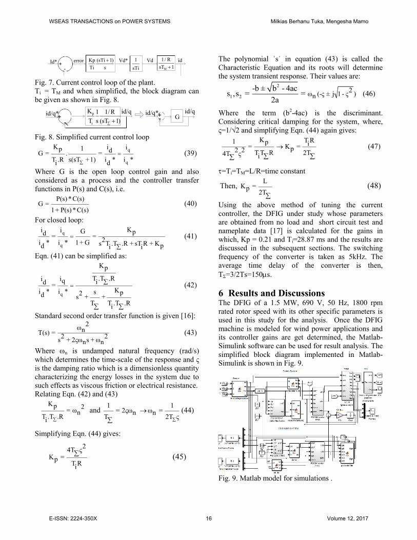
idId*sTi1

1sTR/1

M

error Vd* Vds

)1sTi(TiKp

+-

Fig. 7. Current control loop of the plant. Ti = TM and when simplified, the block diagram can be given as shown in Fig. 8.

id/q*+ )1sT(R/1

s1

TK

i

p

-

id/q id/q*+ G-id/q

Fig. 8. Simplified current control loop

q

q

K i i1p dG = . =T .R s(sT +1) i * i *i d

(39)

Where G is the open loop control gain and also considered as a process and the controller transfer functions in P(s) and C(s), i.e.

P(s) * C(s)G =

1+ P(s) * C(s) (40)

For closed loop: q

q

Ki i G pd = = 2i * i * 1+ G s T .T .R + sT R + Kpd i i

(41)

Eqn. (41) can be simplified as:

q

KpT .T .Rii q id =

Ki * i * s p2d s + +T T .T .Ri

(42)

Standard second order transfer function is given [16]: 2ωnT(s) = 2 2s + 2ςω s + ωn n

(43)

Where n is undamped natural frequency (rad/s) which determines the time-scale of the response and ς is the damping ratio which is a dimensionless quantity characterizing the energy losses in the system due to such effects as viscous friction or electrical resistance. Relating Eqn. (42) and (43)

Kp 2= ω nT .T .Ri

and 1 1

= 2ςω ω =n nT 2T ς

(44)

Simplifying Eqn. (44) gives:

24T ςK =p T Ri

(45)

The polynomial ˈsˈ in equation (43) is called the Characteristic Equation and its roots will determine the system transient response. Their values are:

2

1 22ω (-ς ± j 1 - ς )n

-b ± b - 4acs ,s = =2a

(46)

Where the term (b2-4ac) is the discriminant. Considering critical damping for the system, where, ς=1/√2 and simplifying Eqn. (44) again gives:

K T R1 p i= K =p2 2 T T R 2T4T ς i

(47)

=Ti=TM=L/R=time constant

Then, LK =p 2T

(48)

Using the above method of tuning the current controller, the DFIG under study whose parameters are obtained from no load and short circuit test and nameplate data [17] is calculated for the gains in which, Kp = 0.21 and Ti=28.87 ms and the results are discussed in the subsequent sections. The switching frequency of the converter is taken as 5kHz. The average time delay of the converter is then, T=3/2Ts=150s. 6 Results and Discussions The DFIG of a 1.5 MW, 690 V, 50 Hz, 1800 rpm rated rotor speed with its other specific parameters is used in this study for the analysis. Once the DFIG machine is modeled for wind power applications and its controller gains are get determined, the Matlab-Simulink software can be used for result analysis. The simplified block diagram implemented in Matlab-Simulink is shown in Fig. 9.

Fig. 9. Matlab model for simulations .

WSEAS TRANSACTIONS on POWER SYSTEMS Milkias Berhanu Tuka, Mengesha Mamo

E-ISSN: 2224-350X 16 Volume 12, 2017

6.1. Stability For the purpose of stability analysis of a system, the Bounded Input Bounded Output (BIBO) [16] definition of stability which states that a system is stable if the output remains bounded for all bounded (finite) inputs can be recalled. Substituting, the values of the numerical solutions, the standard second order transfer function form of the plant can be re-written:

p2

d i å n2 2 2

p2d n n

å i å

Ki T .T .R ω 2800326= T(s) = =

Ki * s + 2ςω s + ω s + 6666.67s + 2800326ss + +T T .T .R

Using the Matlab, the poles of the open system are 10^3[-6.2162-i0.4505]. Thus, this system is stable since the real parts of the poles are both negative. In addition, a single real pole at s=0 is positive and non-zeros implies the system’s stablity. Having the factory test report of the machine [17], Fig. 10 is drawn for the comparison of it with the numerical solutions of Fig. 11 [18].

Fig. 10. Factory test results of the DFIG.

Fig. 11. Numerical solution results of the DFIG [20]. Negative real power simply is the indication of generation mode. As it can be seen from Fig.10 and 11, the rotor of the generator receives power (Pr) from

the grid through converters during the subsynchronous mode of operation and sends it during super-synchronous operation, whereas the stator is sending power (Ps) to the grid. The positive value is used here. The grid power which is drawn with positive values of Ps and Pr, in this case, is shown in Fig. 10 and 11. Comparing the grid power with mechanical input power, they are almost following similar behavior with slight deviation due to losses in the system. Fig.12 shows the rotor speed of the machine in rpm at subsynchronous and super synchronous states for the given wind speed. The assumed wind speed used here by repeating sequence of Matlab-Simulink is (4, 6, 11, 11, 6, 4) over the 30 seconds simulation period.

Fig. 12. The rotor speed of the machine. At the rotor speed shown in Fig. 12, the performance analysis of the machine in αβ coordinates when the stator and rotor voltages are injected into the machine as well as with the load torque for the given machine will reach different steady state points are as described here below at sub and super synchronous speeds at specific speeds.

Table 1: Performance Analysis Rotor speed(rpm) 2150 1200 Tem (kNm) 6.14 2 Ps (MW) -0.95 -0.3 Pr (MW) -0.4 0.08 Qs (MW) 0.063 0.024 Qr (MW) -0.162 0.05 Pg (MW) -1.35 -0.2 Pm (MW) -1.4 -0.25

The simulation results over the 30s simulation period are given in Figure 13 (a)-(j).

-2000

-1500

-1000

-500

0

500

1000

1500

2000

0 500 1000 1500 2000 2500

pow

er(k

W)

speed(rpm)

Pg

Pr

Ps

-2500

-2000

-1500

-1000

-500

0

500

1000

1500

2000

2500

0 500 1000 1500 2000 2500

speed(rpm)

pow

er(k

W)

Ps

Pr

speed(rpm)

Ps

Pr

PgPm

WSEAS TRANSACTIONS on POWER SYSTEMS Milkias Berhanu Tuka, Mengesha Mamo

E-ISSN: 2224-350X 17 Volume 12, 2017

(a)

(b)

(c)

(d)

(e)

(f)

(g)

Vs,alpha Vs,betha

Time(s)

vas vbs vcs

Time(s)

WSEAS TRANSACTIONS on POWER SYSTEMS Milkias Berhanu Tuka, Mengesha Mamo

E-ISSN: 2224-350X 18 Volume 12, 2017

(h)

(i)

(j) Fig. 13. A DFIG operation at sub and super synchronous speeds: (a) 3-phase abc stator voltages, (b) 2-phase αβ stator voltages, (c) 3-phase abc stator currents, (d) 2-phase αβ stator currents, (e) 3-phase abc rotor voltages, (f) 2-phase αβ rotor voltages, (g) 3-phase abc rotor currents, (h) 2-phase αβ rotor currents, (i) and (j) are stator and rotor αβ fluxes (Wb). From Fig. 13 (a), (b), (e) and (f), the stator and rotor input voltages are imposed. Near at 7.5 seconds of the simulation period where the wind speed change oc-curred, the rotor voltage is 1800 phase shifted produc-ing the speed change from 1400 rpm (subsynchro-nous) to 2000 rpm (super synchronous). The phase changes are also seen between time periods of 20-30 seconds where again the assumed wind speed is to be changing (see Fig. 13 (e), (f), and Fig.12). On the other hand, the stator voltage is not modified. Both abc and αβ stator voltages have the same pulsa-

tions and equal amplitude. However, the phase of a

rotor voltage is shifting at super synchronism and at sub synchronism.

The αβ stator and rotor fluxes are remaining un-changed during the simulation (Fig. 13i and 13j).

The stator αβ currents have very similar behavior to the stator voltages as they remain constant during the simulation period. In connection, the rotor cur-rents phases remain constant while its abc voltages and currents phases are altering at super-synchronous and sub-synchronous speeds (Fig. 13e-13h).

Fig. 14 shows the simulation result of electromagnetic torque developed.

Fig. 14. Electromechanical torque.

Fig. 15. Stator active power and its reference tracking. The control is imposed through dual converters to track the stator active power and to maintain the reactive power for unity power factor. However, this situation can be modified as per the demand of power utility to be specified at certain limits. Fig. 15. shows us that the PI controller well tracks the stator power to its reference point for optimum power control.

ψr,alpha ψr,betha

Time(s)

ψs,alpha ψs,betha

Time(s)

WSEAS TRANSACTIONS on POWER SYSTEMS Milkias Berhanu Tuka, Mengesha Mamo

E-ISSN: 2224-350X 19 Volume 12, 2017

Fig. 16. Stator active and reactive powers. The stator active power at an assumed wind speed over a simulation period is near 0.95 MW for higher speed and follows the characteristics of the wind. The reactive power is maintained to be controlled at unity power factor. However, there is small deviation at high wind speeds as the machine tries to support the grid with reactive power.

Fig. 17. Rotor active and reactive powers. At super synchronous speed, the rotor and stator ac-tive powers have an equal sign, both negative indicat-ing as the machine is generating. On the other hand, at subsynchronous speed, the rotor active power be-comes positive (due to a positive slip). At this condi-tion, the rotor is receiving power from the grid. The rotor power is near 0.4 MW of power at higher wind speed. It again follows the same pattern as of meas-ured and numeric results discussed before.

Fig. 18. The Grid power. The grid power as the sum of stator and rotor powers neglecting losses is near 1.35 MW in higher wind.

Fig. 19. Comparison of grid and mechanical power. The grid power due to losses is slightly less than the mechanical power. The same situation is shown in Fig. 10 and 11 from calculation results. The efficiency of the machine is simulated with no loss assumption as shown in Fig. 20 and seen better at higher speed.

0 0.5 1 1.5 2 2.5 3

x 104

0

10

20

30

40

50

60

70

80

90

100

Effi

cien

cy(%

)

Time(s)

Fig. 20. Efficiency of the machine.

WSEAS TRANSACTIONS on POWER SYSTEMS Milkias Berhanu Tuka, Mengesha Mamo

E-ISSN: 2224-350X 20 Volume 12, 2017

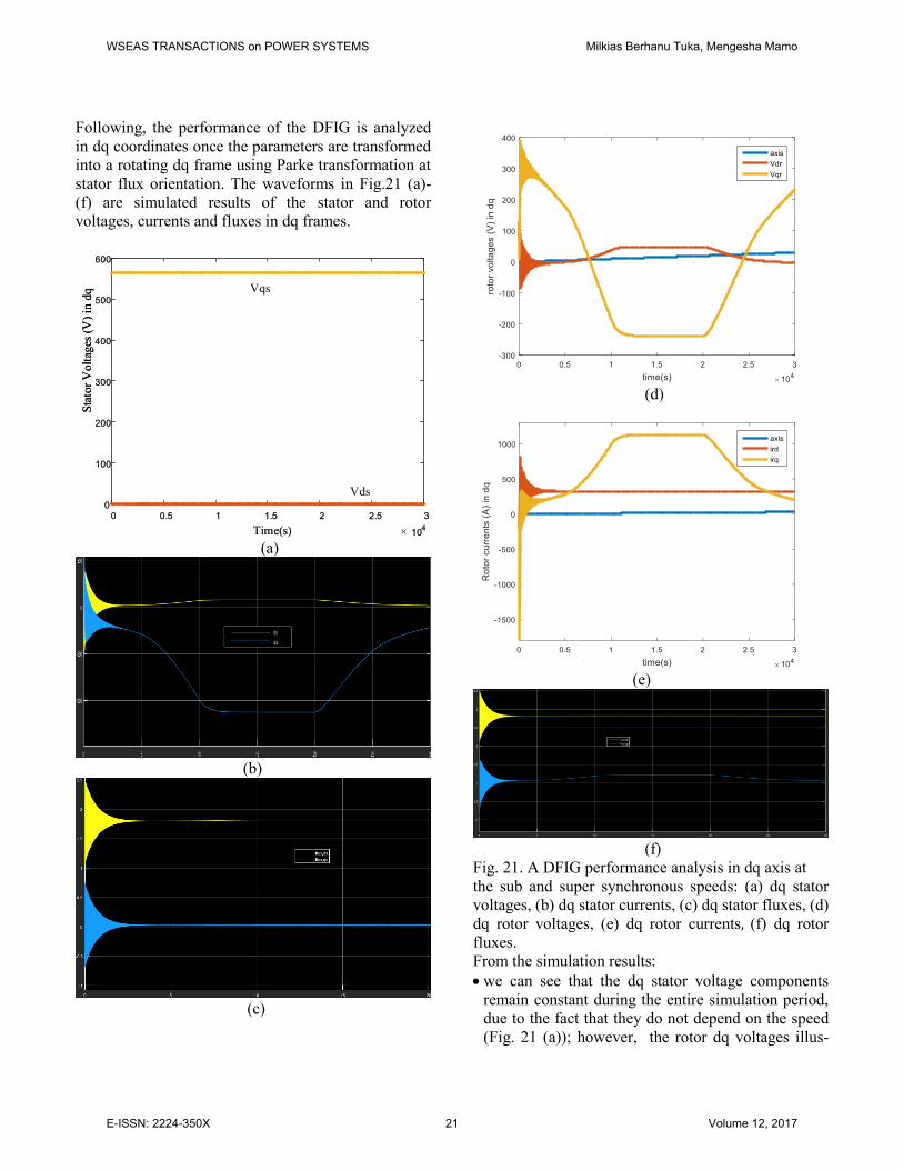
Following, the performance of the DFIG is analyzed in dq coordinates once the parameters are transformed into a rotating dq frame using Parke transformation at stator flux orientation. The waveforms in Fig.21 (a)-(f) are simulated results of the stator and rotor voltages, currents and fluxes in dq frames.

Stat

or V

olta

ges (

V) i

n dq

0 0.5 1 1.5 2 2.5 3

Time(s) 104

0

100

200

300

400

500

600

Vqs

Vds

Stat

or V

olta

ges (

V) i

n dq

0 0.5 1 1.5 2 2.5 3

Time(s) 104

0

100

200

300

400

500

600

Vqs

Vds

(a)

(b)

(c)

(d)

(e)

(f)

Fig. 21. A DFIG performance analysis in dq axis at the sub and super synchronous speeds: (a) dq stator voltages, (b) dq stator currents, (c) dq stator fluxes, (d) dq rotor voltages, (e) dq rotor currents, (f) dq rotor fluxes. From the simulation results: we can see that the dq stator voltage components

remain constant during the entire simulation period, due to the fact that they do not depend on the speed (Fig. 21 (a)); however, the rotor dq voltages illus-

WSEAS TRANSACTIONS on POWER SYSTEMS Milkias Berhanu Tuka, Mengesha Mamo

E-ISSN: 2224-350X 21 Volume 12, 2017

trated in Fig. 21d are modified due to the change of the speed.

the stator d fluxes are constant during the entire simulation regardless of speed changes (Fig. 21c). The q component of the flux is zero since the dq ref-erence frame has been aligned to the stator flux space vector,

the rotor and stator fluxes show similar pattern ex-cept for the q-axis rotor flux slight variation at su-persynchronous speeds (Fig. 21 c and f).

the stator and rotor d currents components remain fixed and q components have an equal pulsation var-iation due to the change of speed (Fig. 21b and e).

7 Conclusion In this paper, the DFIG for its steady state and dynamic operation has been presented. Once the dynamic model has been established, the system is studied for its performance analysis. The numerical analysis, the factory test and simulation results agree with many aspects, however, there exist small deviations in some values due to losses, approximations, and assumptions. The PI controller gains can tune the variables to the desired reference point and hence it is possible to control the rotor currents and hence the active and reactive powers to their respective reference points as per the demand of power authority. Lastly, the modeling gave various pieces of information regarding the performance of the machine and also can give further ideas based on its implementation and need. The model and simulation can also be in different ways. References

[1] G. Cornelis van Kooten, Govinda R. Timilsina, Wind Power Development: Economics and Policies, The World Bank Development Research Group Environment and Energy Team, March 2009 [2] Dr. Jasper Abramowski, Dr. Rolf Posorski, Wind Energy for Developing Countries, DEWI Magazin Nr. 16, Februar 2000 46, GTZ, Germany [3] http://allafrica.com/stories/201505211503.html [online] [4] Tao, Power quality of grid-connected wind tur-

bines with DFIG and their interaction with the grid, PhD dissertation, 2004 [5] N.Pina, J.Kacprzyk, J.FilipeN. Simulation &

Modeling Methodologies, Technologies &

Applications., Advances in intelligent systems and computing, volume 197, 2013 [6] P. Krause, O. Wasynczuk, and S. Sudhoff, Analy-

sis of Electric Machinery and Drive Systems, 2nd Edition, Wiley-IEEE Press, 2002. [7] B. Wu, High-Power Converters and AC Drives, Wiley-IEEE Press, 2006 [8] Haitham Abu-Rub, Mariusz Malinowski and Kamal Al-Haddad, Power Electronics for Renewable

Energy Systems, Transportation and Industrial

Applications, 2014, IEEE Press-John Wiley and Sons Ltd. [9] G. Abad, J. Lo´pez, M. A. Rodri’guez, L. Marroyo, and G. Iwanski, Doubly Fed Induction

Machine: Modeling and Control for Wind Energy

Generation, First Edi.,2011, IEEE Press-John Wiley and Sons Ltd [10] Mohammadi, J.; Vaez-Zadeh, S.; Afsharnia, S.; Daryabeigi, E.“A combined vector and direct power

control for DFIG-Based wind turbines,” IEEE Trans. Sustain. Energy 2014, 5, 767–775. [11] “PID control,” Chapter ten” http://www.cds.caltech.edu/~murray/books/AM08/pdf/am06-pid_16Sep06.pdf [online] [12] Chandra Bajracharya, Control of VSC-HVDC for

wind power, Specialization project, NTNU, 2008. [13] E. S. Ali, Speed control of induction motor supplied by wind turbine via imperialist competitive algorithm, Energy (Elsevier), Vol. 89, September 2015, pp. 593-600. [14] Karl J. Åström and Tore Hägglund, PID

Controllers: Theory, Design, and Tuning, Instrument Society of America, 1995. [15] Remus Teodorescu, Marco Liserre & Pedro Rodríguez, Grid Converters for Photovoltaic and

Wind Power Systems, 2011 John Wiley & Sons, Ltd. [16] Roland S. Burnsm, Advanced Control

Engineering, 2001 [17] Sany DFIG Ethiopia Adama-II wind power project test report‘‘unpublished’’. [18] Milkias Berhanu Tuka, Mengesha Mamo, Steady

state analysis & controlling active and reactive power

of doubly fed induction generator for wind energy

conversion system, IJRES, Volume 1, 2016, ISSN: 2367-9123.

WSEAS TRANSACTIONS on POWER SYSTEMS Milkias Berhanu Tuka, Mengesha Mamo

E-ISSN: 2224-350X 22 Volume 12, 2017