Performance analysis of Alpha-Beta Pruning n Since alpha-beta pruning performs a minimax search while pruning much of the tree, its effect is to allow

Performance analysis of Performance analysis of Alpha-Beta PruningAlpha-Beta Pruning

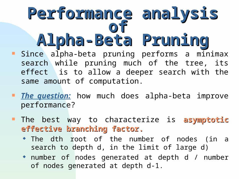
Since alpha-beta pruning performs a minimax search while pruning much of the tree, its effect is to allow a deeper search with the same amount of computation.

The question: how much does alpha-beta improve performance?

The best way to characterize is asymptotic effective asymptotic effective branching factor.branching factor. The dth root of the number of nodes (in a search to depth d,

in the limit of large d) number of nodes generated at depth d / number of nodes

generated at depth d-1.

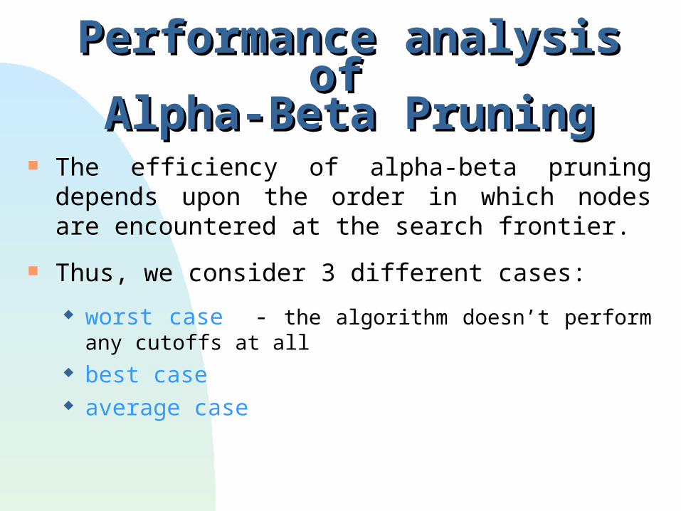
The efficiency of alpha-beta pruning depends upon the order in which nodes are encountered at the search frontier.

Thus, we consider 3 different cases:

worst case - the algorithm doesn’t perform any cutoffs at all best case average case

Performance analysis of Performance analysis of Alpha-Beta PruningAlpha-Beta Pruning

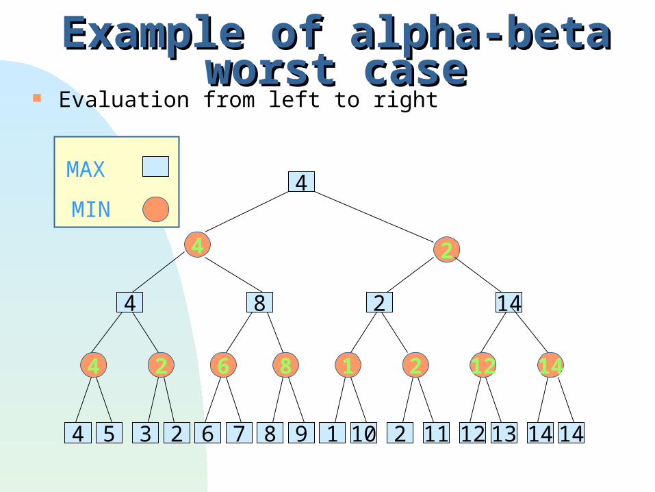
Example of alpha-beta worst caseExample of alpha-beta worst case Evaluation from left to right

4

4 141413121121019876235

1412218624

14284

24

MAX

MIN

Lower Bound for Minimax Lower Bound for Minimax AlgorithmsAlgorithms

We consider a lower bound on the number of leaf nodes that must be examined by any minimax algorithm.

In minimax algorithm, it’s a guaranty to return the minimax value v of the root node of a game tree.

verifying maximum value = v verifying value v && value v.

Any correct minimax algorithm must explore: a strategy for Max a strategy for Min

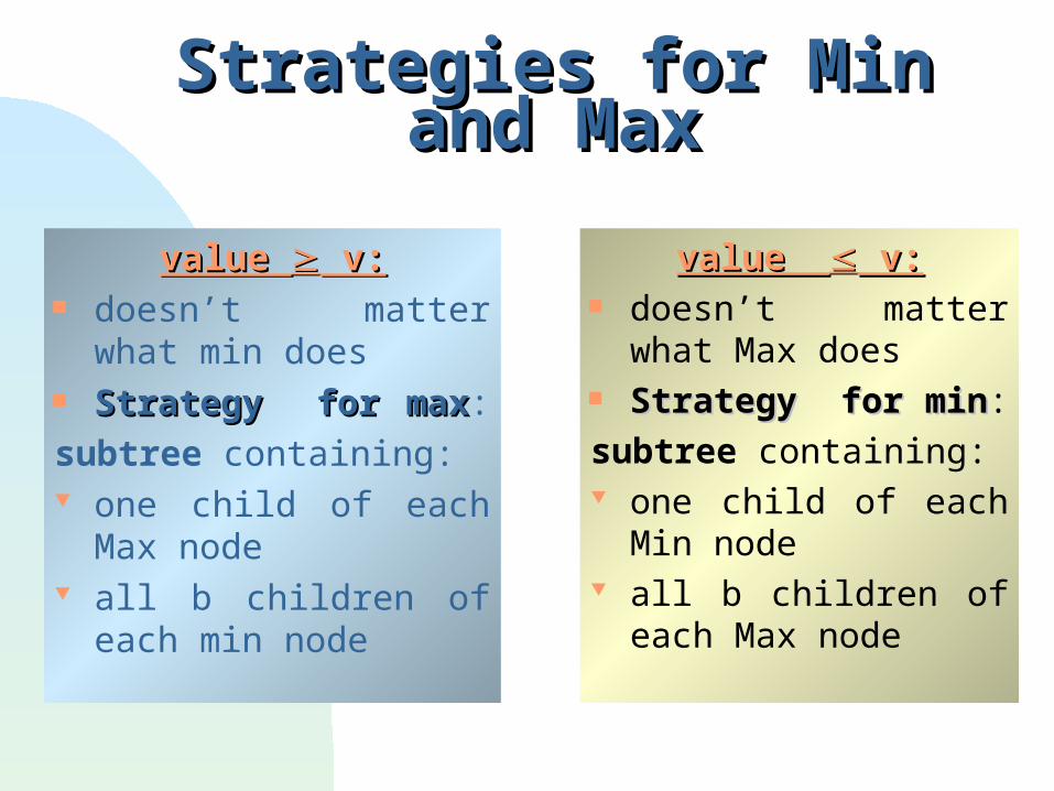
Strategies for Min and MaxStrategies for Min and Max

value value v: v: doesn’t matter what min

does Strategy for maxStrategy for max:

subtree containing: one child of each Max

node all b children of each min

node

value value v: v: doesn’t matter what

Max does Strategy for minStrategy for min:

subtree containing: one child of each Min

node all b children of each

Max node

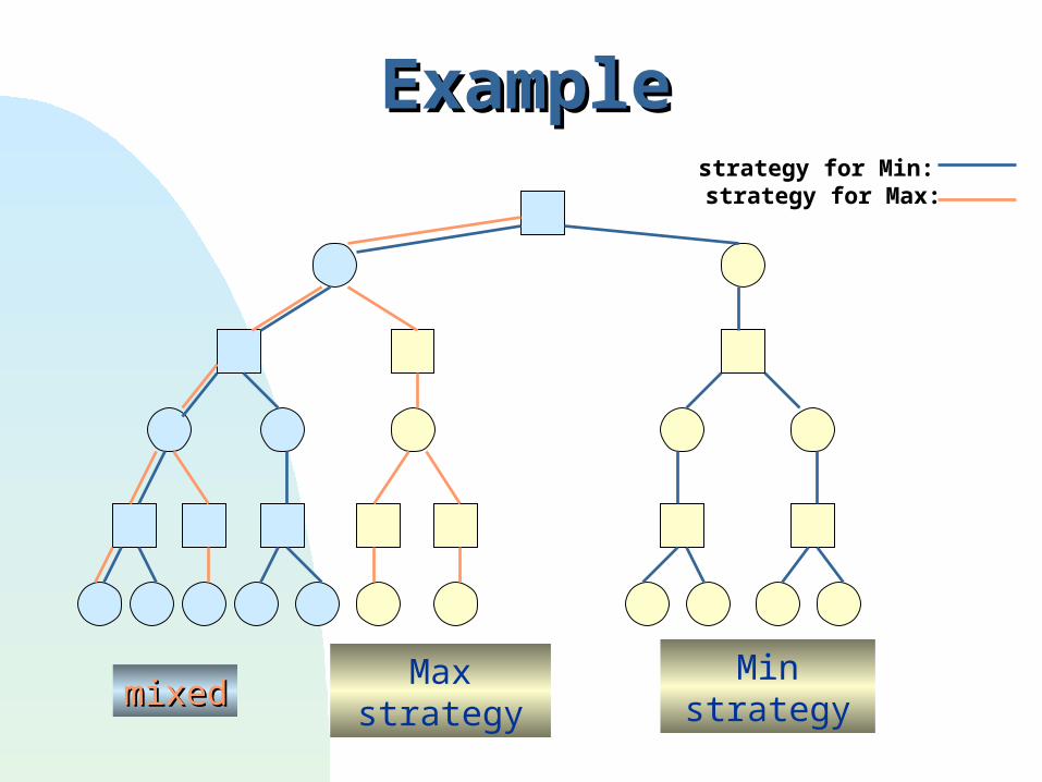
ExampleExample

strategy for Min: strategy for Max:

Max strategy Min strategymixedmixed

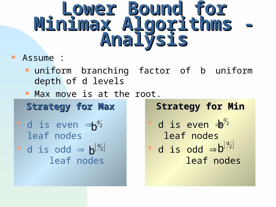
Strategy for MaxStrategy for Max

d is even leaf nodes

d is odd leaf nodes

Strategy for MinStrategy for Min

d is even leaf nodes

d is odd leaf nodes

bd

2

bd

2

bd

2

bd

2

Assume : uniform branching factor of b uniform depth of d levels Max move is at the root.

Lower Bound for Minimax Lower Bound for Minimax Algorithms - AnalysisAlgorithms - Analysis

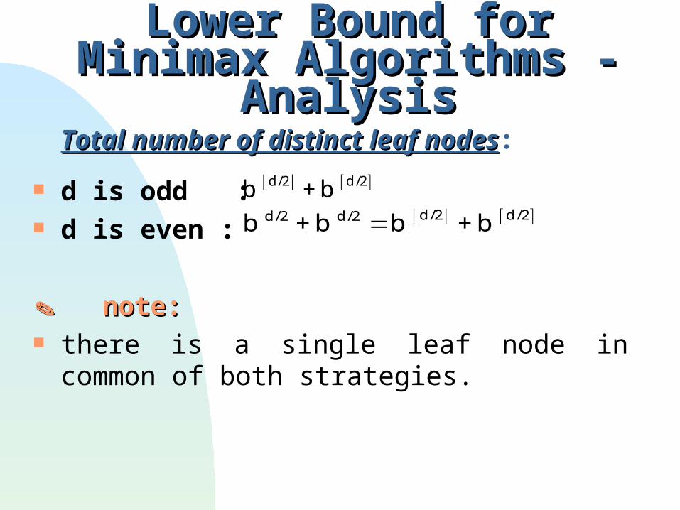
Total number of distinct leaf nodesTotal number of distinct leaf nodes:

d is odd : d is even :

note:note: there is a single leaf node in common of both

strategies.


b + b b + b d/2 d/2 d/2 d/2

b + b d/2 d/2

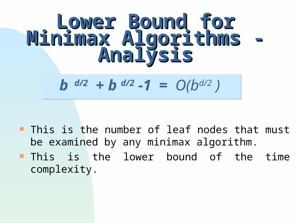
b d/2 + b d/2 -1 = O(bd/2 ) b d/2 + b d/2 -1 = O(bd/2 )

This is the number of leaf nodes that must be examined by any minimax algorithm.

This is the lower bound of the time complexity.


The most natural definition for the average case is that the leaf nodes are randomly ordered.

Heuristic node ordering would violate this assumption.

Average case performance is not a prediction of its performance in practice

Minimax value of game treesMinimax value of game trees

Minimax value of game treesMinimax value of game trees

The root will be in the average case of randomly ordered frontier nodes.

Special case leaf nodes:

are actual terminal positions, have the exact values of WIN or LOSS.

Most general case arbitrary leaf node values

WIN-LOSS Trees analytic modelWIN-LOSS Trees analytic model

uniform branching factor b uniform depth d Max is to move at the root depth d is even terminal nodes labeled WIN with probability P0

terminal nodes labeled LOSS with probability 1 - P0

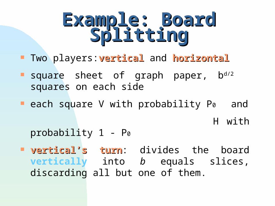
Example: Board SplittingExample: Board Splitting

Two players:verticalvertical and horizontalhorizontal

square sheet of graph paper, bd/2 squares on each side

each square V with probability P0 and

H with probability 1 - P0

vertical’svertical’s turnturn: divides the board vertically into b equals slices, discarding all but one of them.

horizontal’s turnhorizontal’s turn: divides the board

horizontally into b equals slices, discarding all but one of them.

ResultResult: the initial in the only square left indicates the winner.

Board SplittingBoard Splitting

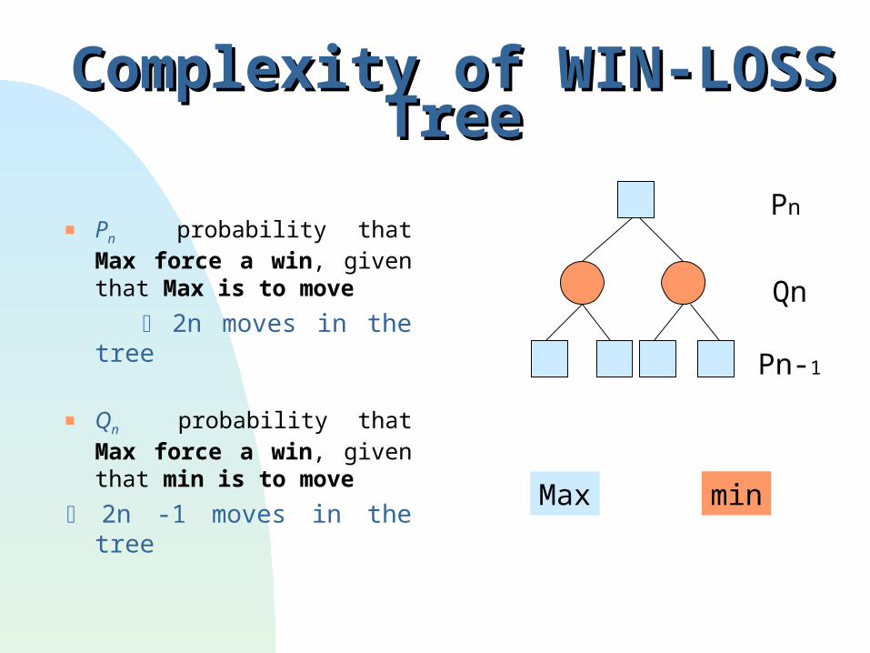
Complexity of WIN-LOSS TreeComplexity of WIN-LOSS Tree

Pn probability that Max force a win, given that Max is to move

2n moves in the tree

Qn probability that Max force a win, given that min is to move

2n -1 moves in the tree

Pn

Qn

Pn-1

Max min

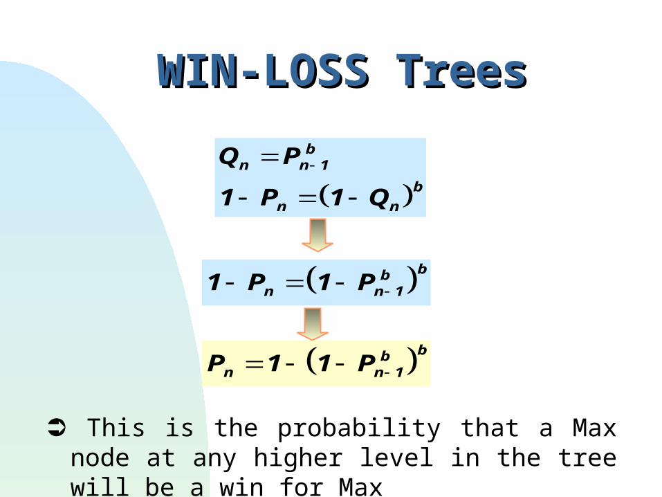
Q P

1 P 1 Q

n n 1b

n n

b

1 P 1 Pn n 1b b

P 1 1 Pn n 1b b

This is the probability that a Max node at any higher level in the tree will be a win for Max

WIN-LOSS TreesWIN-LOSS Trees

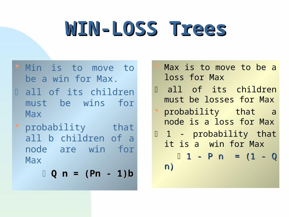
Min is to move to be a

win for Max.

all of its children must be wins for Max

probability that all b children of a node are win for Max

Q n = (Pn - 1)bQ n = (Pn - 1)b

Max is to move to be a loss for Max

all of its children must be losses for Max

probability that a node is a loss for Max

1 - probability that it is a win for Max

1 - P n = (1 - Q n)1 - P n = (1 - Q n)


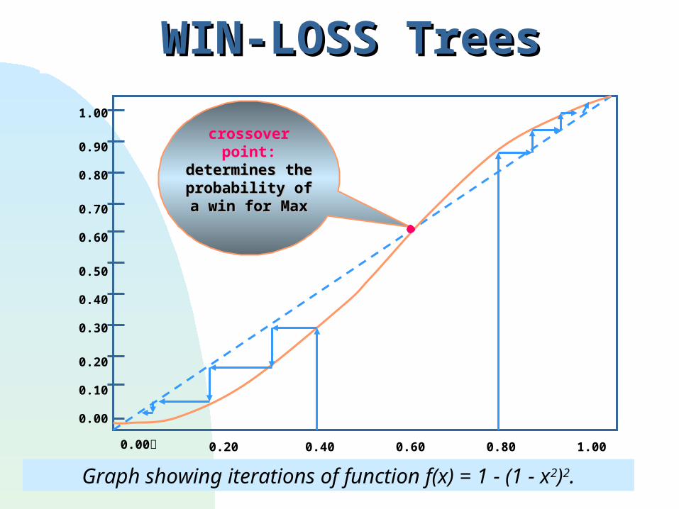
Graph showing iterations of function f(x) = 1 - (1 - x2)2.


ב0.00 0.20 0.40 0.60 0.80 1.00

0.00

0.10

0.20

0.30

0.40

0.50

0.60

0.70

0.80

0.90

1.00

crossover point: determines the determines the

probability of a win probability of a win for Maxfor Max


If the probability of a win for MAX at the leaves is grater than crossover point, then the large enough game tree is almost certainly a forced win for MAX!

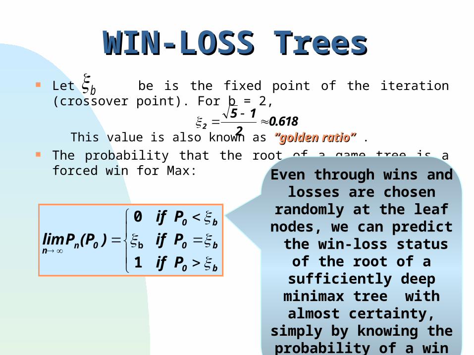
Let be is the fixed point of the iteration (crossover point). For b = 2,

This value is also known as “golden ratio”“golden ratio” . The probability that the root of a game tree is a forced win for Max:


2

5 1

20.618

lim P (P )

if P

if P

if Pn

n 0

0 b

0 b

0 b

0

1b

b

Even through wins and losses are chosen randomly at the leaf nodes, we can predict the win-

loss status of the root of a sufficiently deep minimax tree with almost certainty, simply by knowing the probability of a win

at the leaves!

Minimax convergence theoremMinimax convergence theorem

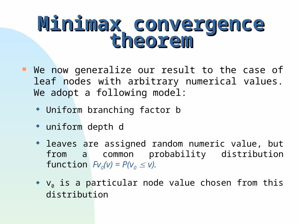
We now generalize our result to the case of leaf nodes with arbitrary numerical values. We adopt a following model:

Uniform branching factor b

uniform depth d

leaves are assigned random numeric value, but from a common probability distribution function Fv0(v) = P(v0 v).

v0 is a particular node value chosen from this distribution

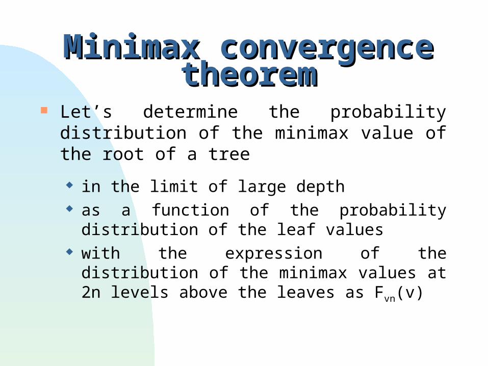
Let’s determine the probability distribution of the minimax value of the root of a tree

in the limit of large depth as a function of the probability distribution of the

leaf values with the expression of the distribution of the

minimax values at 2n levels above the leaves as Fvn(v)


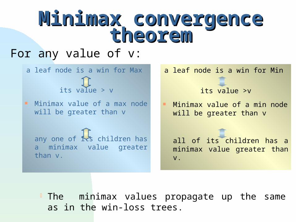
For any value of v:

The minimax values propagate up the same as in the win-loss trees.


a leaf node is a win for Min

its value >v

Minimax value of a min node will be greater than v

all of its children has a minimax value greater than v.

a leaf node is a win for Max

its value > v

Minimax value of a max node will be greater than v

any one of its children has a minimax value greater than v.

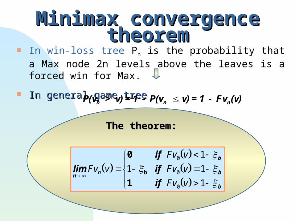
In win-loss tree Pn is the probability that a Max node 2n levels above the leaves is a forced win for Max.

In general game treeIn general game tree


P(v > v) = 1 - P(v v) = 1 - Fv (v)n n n

lim

if

if

ifn

b

b

b

Fv v

Fv v

Fv v

Fv vn

0

1b1

1

1

1

0

0

0

The theorem:The theorem:

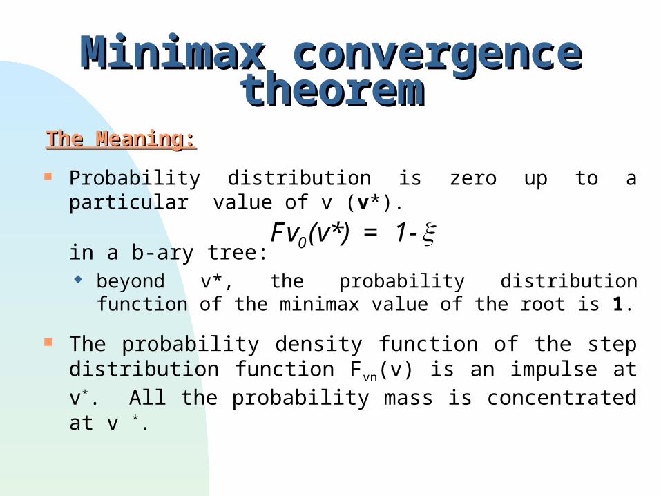
The Meaning:The Meaning:

Probability distribution is zero up to a particular value of v (v*).

in a b-ary tree: beyond v*, the probability distribution function of the

minimax value of the root is 1.

The probability density function of the step distribution function Fvn(v) is an impulse at v*. All the probability mass is concentrated at v *.


Fv (v*) = 1- 0

Conclusion for a minimax tree Conclusion for a minimax tree

We can predict exactly what the minimax value of the root of the tree will be.

Given: arbitrary terminal values chosen independently from

the same distribution limit of large depth

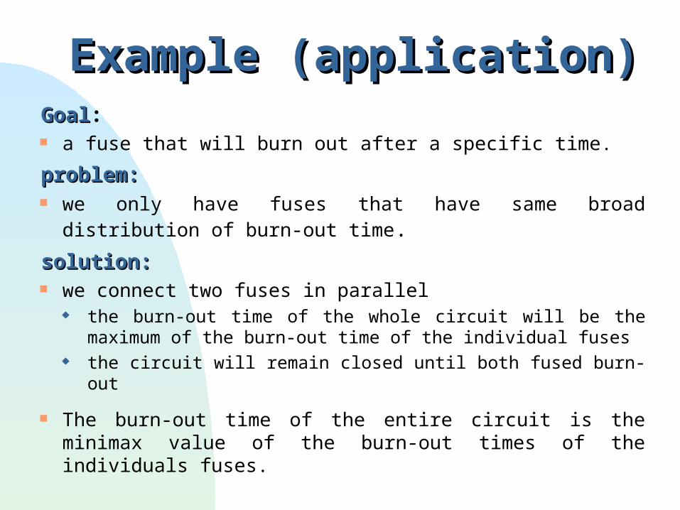
GoalGoal: a fuse that will burn out after a specific time.

problem:problem: we only have fuses that have same broad distribution of

burn-out time.

solution:solution: we connect two fuses in parallel

the burn-out time of the whole circuit will be the maximum of the burn-out time of the individual fuses

the circuit will remain closed until both fused burn-out

The burn-out time of the entire circuit is the minimax value of the burn-out times of the individuals fuses.

Example (application)Example (application)

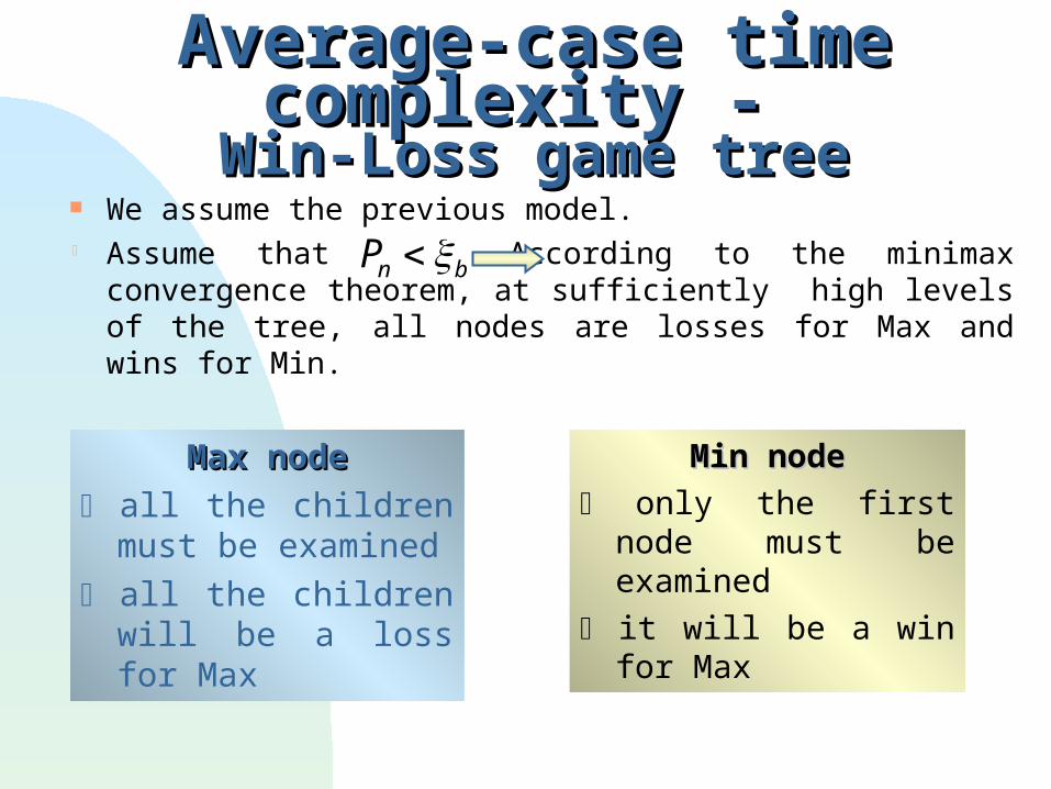
Average-case time complexity - Average-case time complexity - Win-Loss game treeWin-Loss game tree

We assume the previous model. Assume that According to the minimax

convergence theorem, at sufficiently high levels of the tree, all nodes are losses for Max and wins for Min.

Pn b

Max nodeMax node

all the children must be examined

all the children will be a loss for Max

Min nodeMin node

only the first node must be examined

it will be a win for Max

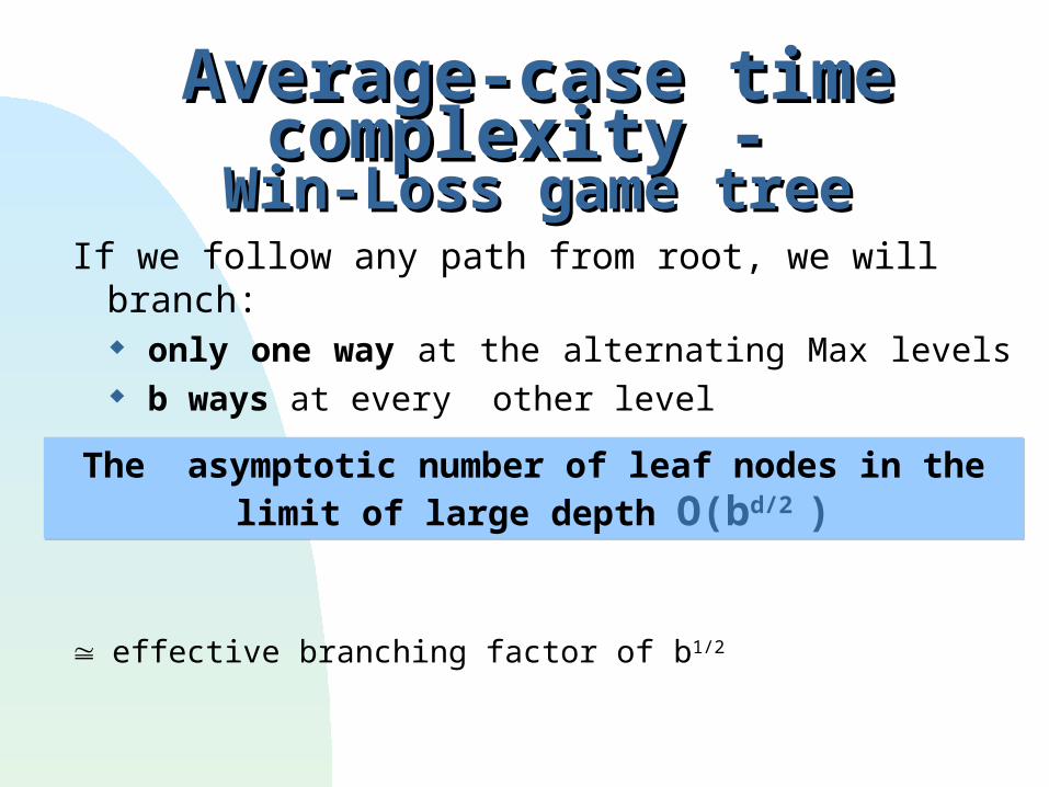
If we follow any path from root, we will branch: only one way at the alternating Max levels b ways at every other level

effective branching factor of b1/2


The asymptotic number of leaf nodes in the limit of large depth O(bd/2 )

The asymptotic number of leaf nodes in the limit of large depth O(bd/2 )

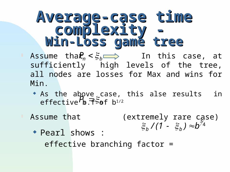
Assume that In this case, at sufficiently high levels of the tree, all nodes are losses for Max and wins for Min. As the above case, this alse results in effective b.f of b1/2

Assume that (extremely rare case)

Pearl shows :effective branching factor =


Pn b

Pn b

b / (1 - ) b b

34

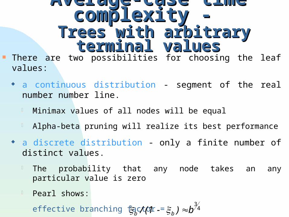
There are two possibilities for choosing the leaf values:

a continuous distribution - segment of the real number number line.

Minimax values of all nodes will be equal

Alpha-beta pruning will realize its best performance

a discrete distribution - only a finite number of distinct values.

The probability that any node takes an any particular value is zero

Pearl shows:

effective branching factor =

Average-case time complexity - Average-case time complexity - Trees with arbitrary terminal valuesTrees with arbitrary terminal values

b / (1 - ) b b

34

We generalize the 2-player-perfect-information algorithms, to the case of non-cooperative perfect-information -more players games.

No coalitions between players.

ExamplesExamples:

Chinese Checkers with 6 players. Othello extended by having different colored

pieces for each player.

IntroductionIntroduction

Maxn (maxMaxn (maxnn) Algorithm) Algorithm

AssumptionAssumption:

the players alternate moves

each player tries to maximize his/her return

and indifferent to returns of others.

At frontier nodes, evaluation function returns an n-tuple of values:

(player1, P2, P3, …. Player n)

For example:For example:

Othello - return number of pieces for each player.

Maxn AlgorithmMaxn Algorithm

the entire n-tuple of the child for which the ith component is maximum.

the entire n-tuple of the child for which the ith component is maximum.


evaluation function in each interior node where player i is to move

evaluation function in each interior node where player i is to move

=

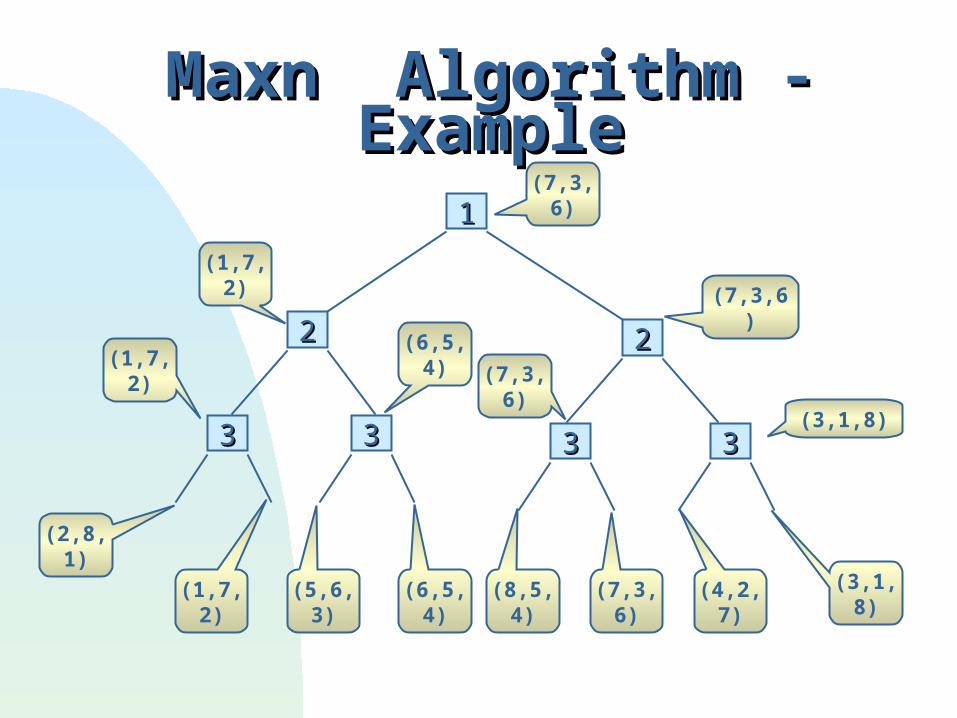
Maxn Algorithm - ExampleMaxn Algorithm - Example

11

22

3333

22

33 33

(7,3,6)

(7,3,6)

(3,1,8)

(6,5,4)

(7,3,6)

(1,7,2)

(1,7,2)

(2,8,1)

(1,7,2) (5,6,3) (6,5,4) (8,5,4) (7,3,6) (4,2,7) (3,1,8)

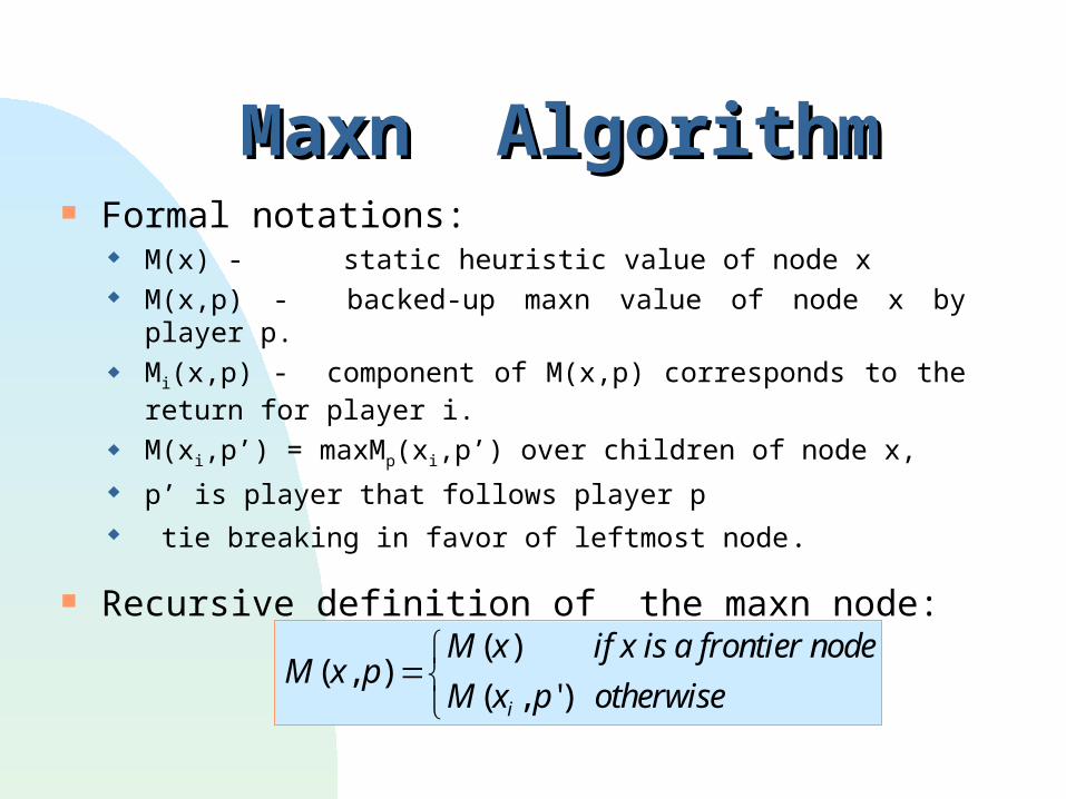
Formal notations: M(x) - static heuristic value of node x M(x,p) - backed-up maxn value of node x by player p. Mi(x,p) - component of M(x,p) corresponds to the return for

player i. M(xi,p’) = maxMp(xi,p’) over children of node x,

p’ is player that follows player p tie breaking in favor of leftmost node.

Recursive definition of the maxn node:


M x pM x

x pi

( , )( )

( , ' )M

if x is a frontier node

otherwise

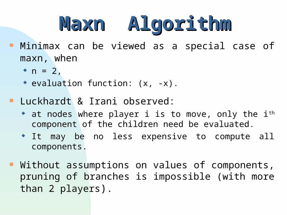
Minimax can be viewed as a special case of maxn, when n = 2, evaluation function: (x, -x).

Luckhardt & Irani observed: at nodes where player i is to move, only the i th component

of the children need be evaluated. It may be no less expensive to compute all components.

Without assumptions on values of components, pruning of branches is impossible (with more than 2 players).


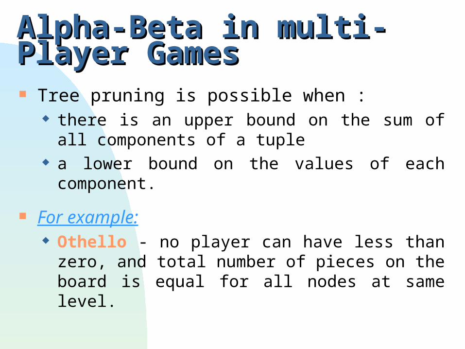
Tree pruning is possible when : there is an upper bound on the sum of all

components of a tuple a lower bound on the values of each component.

For example: Othello - no player can have less than zero, and

total number of pieces on the board is equal for all nodes at same level.

Alpha-Beta in multi-Player GamesAlpha-Beta in multi-Player Games

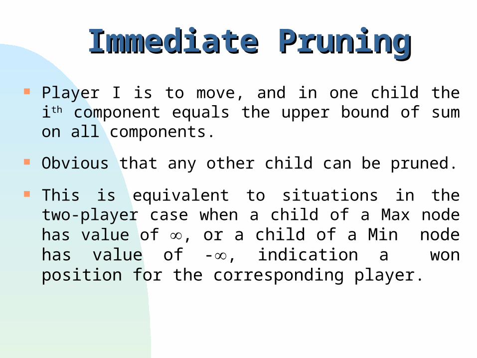
Immediate PruningImmediate Pruning Player I is to move, and in one child the ith component

equals the upper bound of sum on all components.

Obvious that any other child can be pruned.

This is equivalent to situations in the two-player case when a child of a Max node has value of , or a child of a Min node has value of -, indication a won position for the corresponding player.

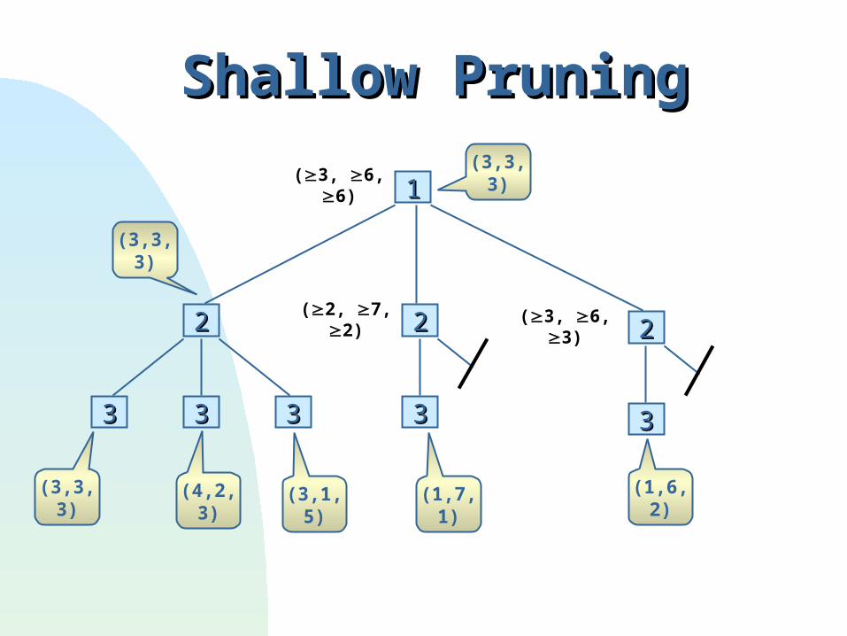
Shallow PruningShallow Pruning

11(3,3,3)

22

33

22

3333 33

22

33

(3,3,3)

(3,3,3) (4,2,3) (3,1,5) (1,7,1) (1,6,2)

(3, 6, 6)

(2, 7, 2)

(3, 6, 3)

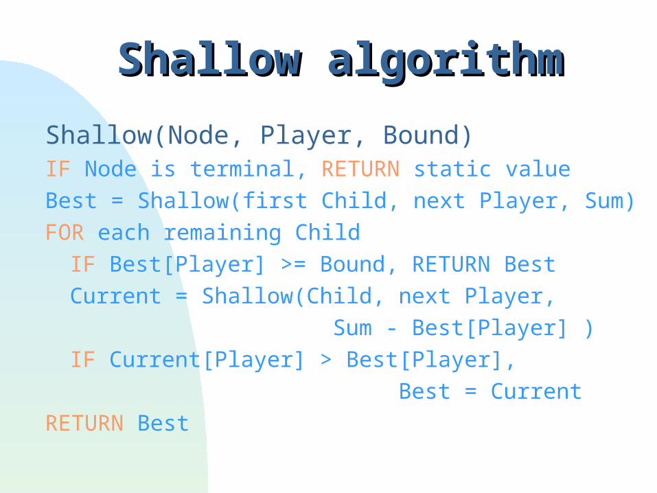
Shallow(Node, Player, Bound)IF Node is terminal, RETURN static value

Best = Shallow(first Child, next Player, Sum)

FOR each remaining Child

IF Best[Player] >= Bound, RETURN Best

Current = Shallow(Child, next Player,

Sum - Best[Player] )

IF Current[Player] > Best[Player],

Best = Current

RETURN Best

Shallow algorithmShallow algorithm

Failure of deep pruningFailure of deep pruning

In a 2-player game, alpha-beta allows deep pruning - pruning a node based on bounds inherited from its great-grandparents, or other distant ancestor.

Deep pruning does not generalize to more than 2 players!

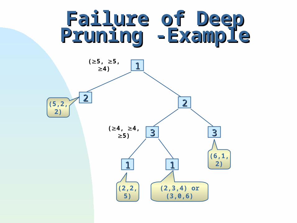
Failure of Deep Pruning -ExampleFailure of Deep Pruning -Example

11

2222

33

1111

33

(5, 5, 4)

(4, 4, 5)

(5,2,2)

(6,1,2)

(2,2,5) (2,3,4) or (3,0,6)

Theorem: Every directional algorithm that computes the maxn

value of a game tree with more than 2 players must evaluate every terminal node evaluated by shallow pruning under the same order.

Steps of proof:Steps of proof: The formal proof is by induction on the height of

the tree and generalizes the result to an arbitrary number of players greater than 2.

Optimality of shallow pruningOptimality of shallow pruning

Try to see a “zipper” effect in the sense that the original order of the “teeth” (nodes) at the bottom determines the order of the teeth at the top, even though no individual tooth can move very far.

Optimality of shallow pruningOptimality of shallow pruning

Minimax and PathologyMinimax and Pathology

So far, we have considered the time and spacre complexities of minimax search.

We now turn our attention to the quality of the decisions it makes.

Since alpha-beta makes exactly the same decisions as minimax search, the question is the decision quality of minimax.

Exact Terminal ValuesExact Terminal Values If the leaf nodes of the tree are evaluated

exactly,the minimax makes optimal moves against an opponent who plays perfectly.

But decision quality is not optimal against an imperfect opponent, who can make mistakes.

Example of situation:Example of situation: two moves are available:

- may lead easily and immediately to loss - require a long sequence of moves and great

deal of skill of the opponent to force the loss. Minimax has no preference for one option over the other.

Exact Terminal Values - ExampleExact Terminal Values - Example Against an infallible opponent, it does no matter

what move is made.

Against an opponent who can make mistakes, it is far preferable to choose the move that requires the most skill on the part of opponent, increasing the chances of an error by the opponent - and hence a win by the player to move.

Minimaxing of Heuristic valuesMinimaxing of Heuristic values With the exception of the endgame, the values

associated with most nodes in a game are heuristic values returned by the static evaluation.

To decrease an error, the heuristic values should be maximized up as if they were exact values.

Minimaxing of Heuristic values-Minimaxing of Heuristic values-ExampleExample

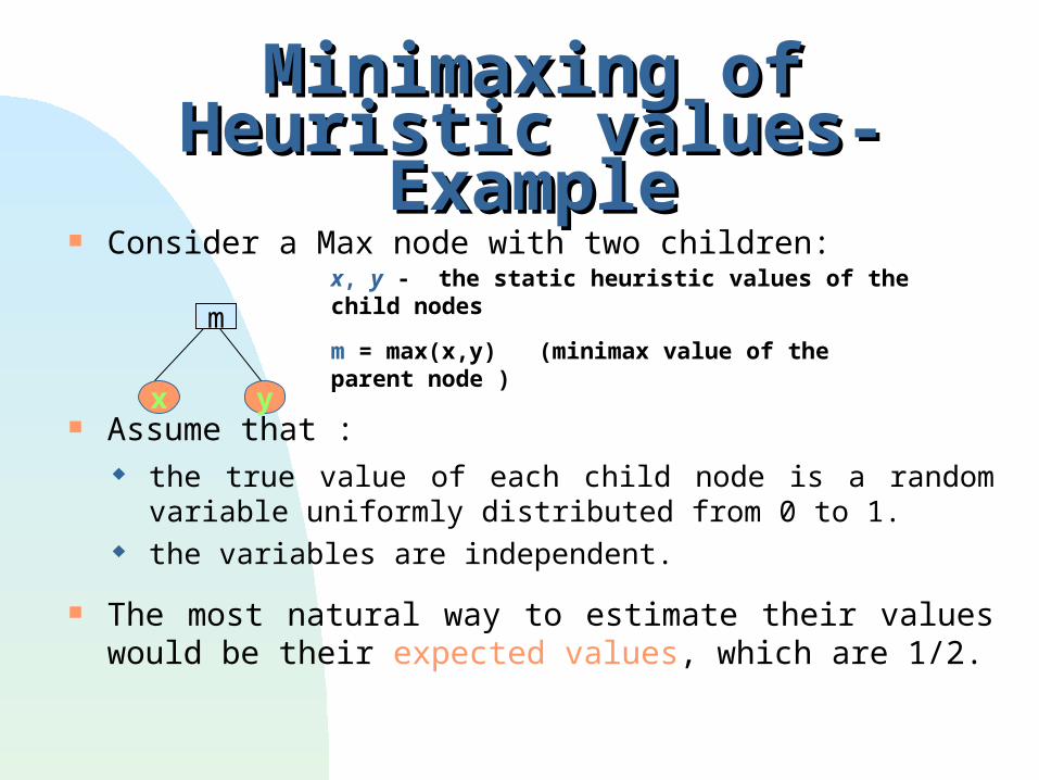
Consider a Max node with two children:

Assume that : the true value of each child node is a random variable

uniformly distributed from 0 to 1. the variables are independent.

The most natural way to estimate their values would be their expected values, which are 1/2.

yx

m x, y - the static heuristic values of the child nodes

m = max(x,y) (minimax value of the parent node )

Minimaxing of Heuristic values-Minimaxing of Heuristic values-ExampleExample

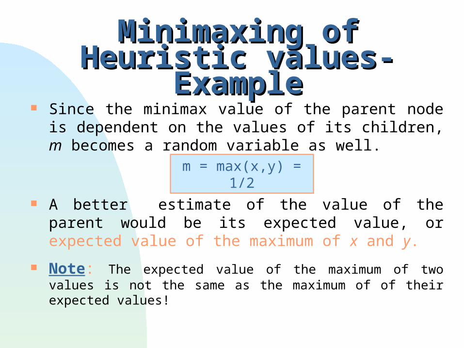
Since the minimax value of the parent node is dependent on the values of its children, m becomes a random variable as well.

A better estimate of the value of the parent would be its expected value, or expected value of the maximum of x and y.

Note: The expected value of the maximum of two values is not the same as the maximum of of their expected values!

m = max(x,y) = 1/2

Minimaxing of Heuristic values-Minimaxing of Heuristic values-ProofProof

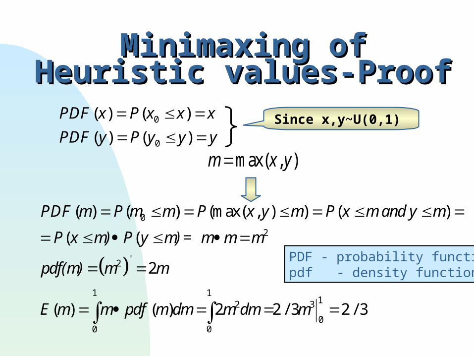
PDF x P x x x

PDF y P y y y

( ) ( )

( ) ( )

0

0

Since x,y~U(0,1)

m x ymax( , )

PDF m P m m P x y m P x m

P x P y m m

m m

E m m pdf m dm m dm m

( ) ( ) (max( , ) ) ( )

( (

( ) ( ) / /

'

0

2

2

0

12

0

13

0

1

2

2 2 3 2 3

m and y

m) m)= m

pdf(m)PDF - probability functionpdf - density function

Minimaxing of Heuristic valuesMinimaxing of Heuristic values Thus, the expected value of the maximum of two

random variables chosen independently from the uniform distribution from 0 to 1 is 2/3, while the maximum of their expected values is only 1/2.

The essential error of minimax is is to take the maximum/minimum of the expected values instead of computing the expected value of the maximum/minimum.

As the search deeper, the minimax value accumulate more and more error.

Minimaxing of Heuristic valuesMinimaxing of Heuristic values Why not to compute the exact value of the root of a

game tree?

This requires the exact distribution function of all of our leaf nodes, which we don’t know in a real game.

To do the above calculation, we assumed that the values of the child nodes were independent of one another, which is unlikely to be true in a real game.

Even if we had the exact distribution and they were independent, the distributions of interior nodes become increasingly complex functions and can be calculated exactly only in small trees.

Game tree pathologyGame tree pathology The above error in maximizing gives rise to an effect

known as game-tree pathologygame-tree pathology.

In the board-splitting game tree, the decision quality of minimax as a function of search depth increases with increasing depth, up to a point, Beyond a certain depth, the percentage of optimal moves made by minimax searching deeper it less than for minimax searching to a shallower depth.

The meaning:

The error propagation due to maximizing overcomes the additional information derived from searching deeper.

The error propagation due to maximizing overcomes the additional information derived from searching deeper.

Game tree pathologyGame tree pathology

In real games, searching deeper almost never results in poorer overall quality of play.

The puzzle then is to determine what is about board splitting that causes it to be pathological, unlike real games.

There are several possible explanations.

Game tree pathology - Possible Game tree pathology - Possible ReasonsReasons

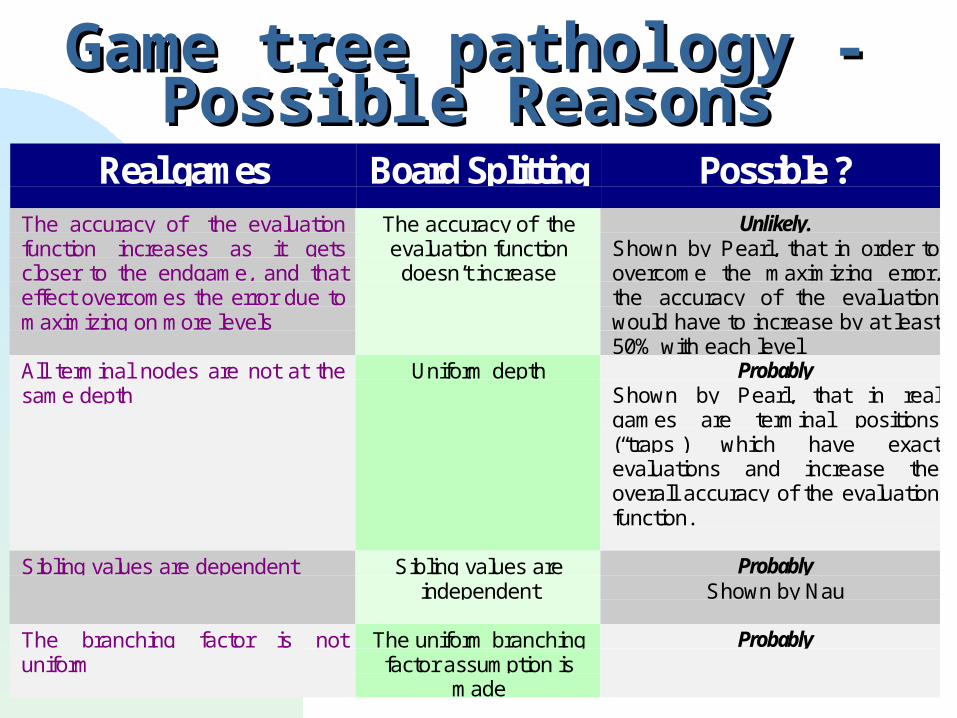
Real games Board Splitting Possible ?

The accuracy of the evaluationfunction increases as it getscloser to the endgame, and thateffect overcomes the error due tomaximizing on more levels

The accuracy of theevaluation functiondoesn’t increase

Unlikely.Shown by Pearl, that in order toovercome the maximizing error,the accuracy of the evaluationwould have to increase by at least50% with each level

All terminal nodes are not at thesame depth

Uniform depth ProbablyShown by Pearl, that in realgames are terminal positions(“traps”) which have exactevaluations and increase theoverall accuracy of the evaluationfunction.

Sibling values are dependent Sibling values are

independentProbably

Shown by Nau

The branching factor is notuniform

The uniform branchingfactor assumption is

made

Probably

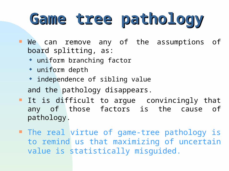
We can remove any of the assumptions of board splitting, as: uniform branching factor uniform depth independence of sibling value

and the pathology disappears. It is difficult to argue convincingly that any of those

factors is the cause of pathology.

The real virtue of game-tree pathology is to remind us that maximizing of uncertain value is statistically misguided.

Game tree pathologyGame tree pathology

We turn our attention to the problem of learning heuristic functions for two-player games.

The most obvious, and still most commonly used technique, is hand-coding by a human expert.

Example: Deep_blue(chess) Chinook’s(checkers).

Learning Two Player Evaluation Learning Two Player Evaluation FunctionsFunctions

Arthur Samuel’s checkers program, written in the 1950’s.

In 1962, running on an IBM 7094, the machine defeated R.W.Nealy, a future Connecticut state checkers champion.

One of the first machine learning programs, introducing a number of different learning techniques.

Samuel’s Checker PlayerSamuel’s Checker Player


Rote LearningRote Learning

When a minimax value is computed for a position, that position is stored along with its value.

If the same position is encountered again, the value can simply be returned.

Due to memory constraints, all the generated board position cannot be stored, and Samuel used a set of criteria for determining which positions to actually store.

Learning the evaluation functionLearning the evaluation function

Comparing the static evaluation of a node with the backed-up minimax value from a lookahead search.

If the heuristic evaluation function is perfect, the static value of a node would be equal to the backed-up value based on a lookahead search applying the same evaluation on the frontier nodes.

If there’s a difference between the values, the evaluation the heuristic function should be modified.


Selecting termSelecting term Samuel’s program could select which terms to

actually use, from a librarylibrary of possible terms. In addition to material, these terms attempted to

measure following board features : center control advancement of the pieces mobility

The program computes the correlation between the values of these different features and the overall evaluation score. If the correlation of a particular feature dropped below a certain level, the feature was replaced by another.


Samuel’s method for modifying the weights were somewhat Ad Hoc.

We shell describe a more principled way of performing this task.

Linear RegressionLinear Regression

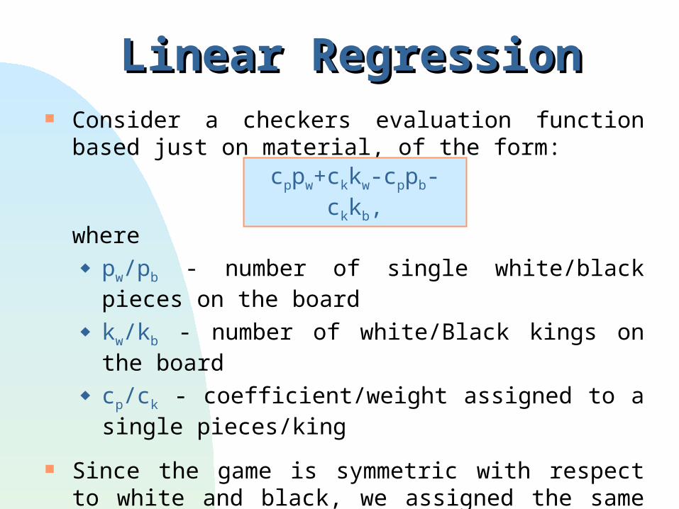
Consider a checkers evaluation function based just on material, of the form:

where pw/pb - number of single white/black pieces on the

board kw/kb - number of white/Black kings on the board

cp/ck - coefficient/weight assigned to a single pieces/king

Since the game is symmetric with respect to white and black, we assigned the same pieces the same weights.


cppw+ckkw-cppb-ckkb,

An individual function is represented by a particular set of values for cp and ck.

We represent all such function in a two dimensional space with cp on one axis and ck on the other.

our task: to find the best point in this space.

We start with an initial approximation of the relative weights and find out from the equation the static heuristic value of the current state.


From this game state, We perform a lookahead search as deeply as

our computational resources allow. At the frontier, our current evaluation function

is applied to the leaf nodes, and these values are minimaxed back up to the root to determine a backed up value b for the position.

In general, this value will not equal the static value of the node.


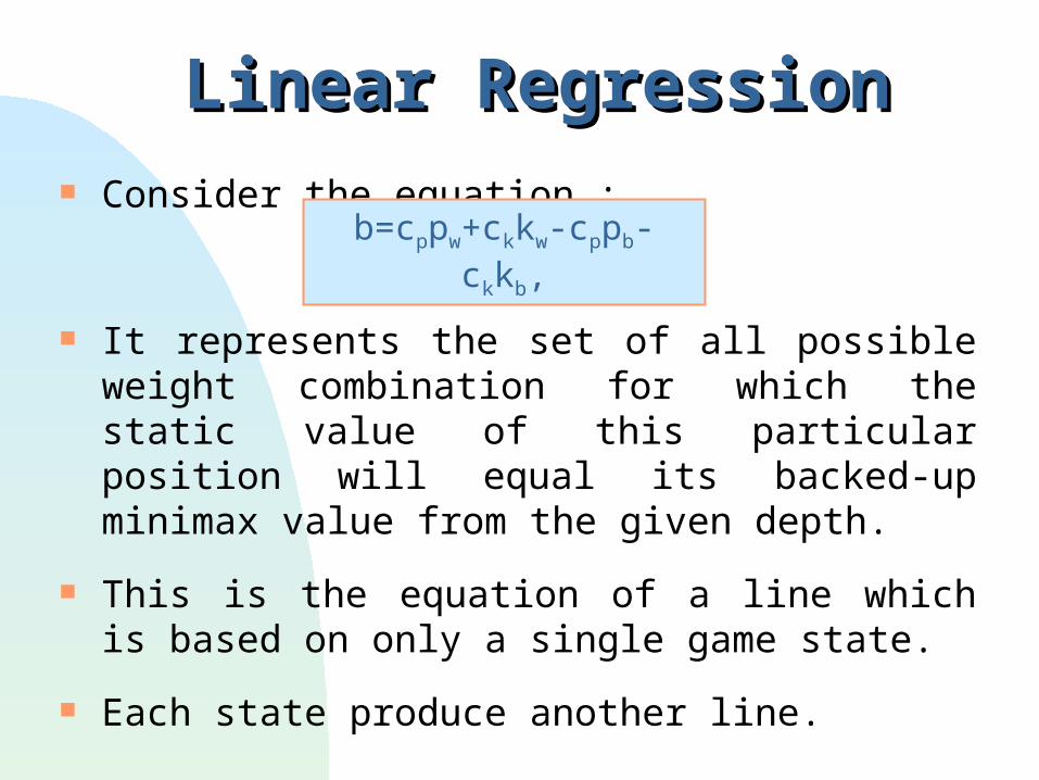
Consider the equation :

It represents the set of all possible weight combination for which the static value of this particular position will equal its backed-up minimax value from the given depth.

This is the equation of a line which is based on only a single game state.

Each state produce another line.


b=cppw+ckkw-cppb-ckkb,

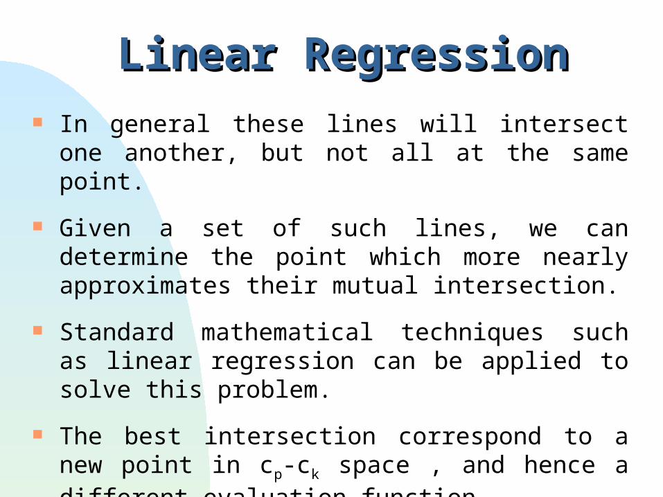
In general these lines will intersect one another, but not all at the same point.

Given a set of such lines, we can determine the point which more nearly approximates their mutual intersection.

Standard mathematical techniques such as linear regression can be applied to solve this problem.

The best intersection correspond to a new point in cp-ck space , and hence a different evaluation function.


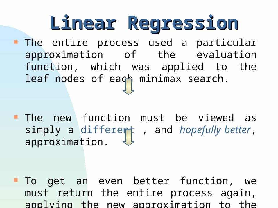
The entire process used a particular approximation of the evaluation function, which was applied to the leaf nodes of each minimax search.

The new function must be viewed as simply a different , and hopefully better, approximation.

To get an even better function, we must return the entire process again, applying the new approximation to the leaf nodes to get yet another approximation.


We have two loops to this process.

the inner loopthe inner loop uses a particular evaluation function to derive a new approximation.

the outer loopthe outer loop iterates this process over multiple approximation.

Hopefully it will eventually converge to a particular function or a small neighborhood of such function.


As a test of these ideas, was the task of learning the relative weights of the different chess pieces.

The evaluation function was based purely on material, with five parameters - the weights of :

queens rooks bishops knights pawns

Experiments with ChessExperiments with Chess

Initially all weights were set to one.

The lookahead search was limited to two levels deep, and linear regression was used to derive each successive approximation to the evaluation function.

Surprisingly, the values eventually converged to a fixed point.

Experiments with ChessExperiments with Chess

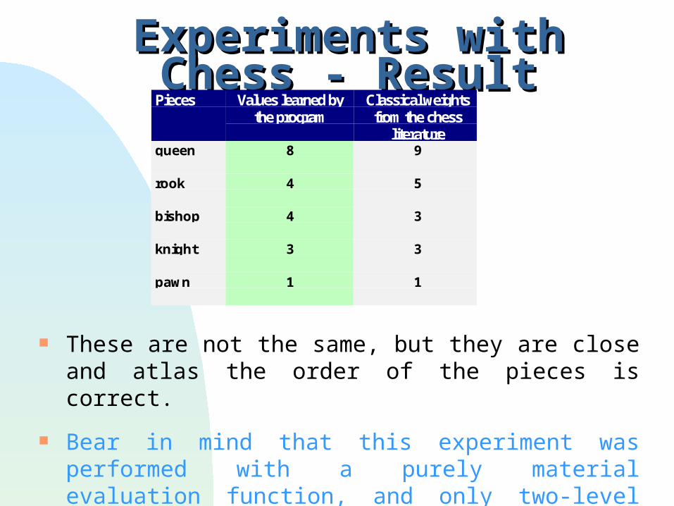
These are not the same, but they are close and atlas the order of the pieces is correct.

Bear in mind that this experiment was performed with a purely material evaluation function, and only two-level lookahead !

Experiments with Chess - ResultExperiments with Chess - ResultPieces Values learned by

the programClassical weights

from the chessliterature

queen 8 9

rook 4 5

bishop 4 3

knight 3 3

pawn 1 1

Documents

Performance analysis of Alpha-Beta Pruning n Since alpha-beta pruning performs a minimax search while pruning much of the tree, its effect is to allow