In/tormurion Swems Vol. 15. NO. 3. pp. 281-290. 1990 03064379 90 S3.M) + 0.00 Printed in Great Bntain. All rights reserved Copyright c I990 Pergamon Press plc

PERFECT HASHING USING SPARSE MATRIX PACKING

MARSHALL D. BRAIN and ALAN L. THARP

Computer Science Department, North Carolina State University, Raleigh, NC 276954206. U.S.A.

(Receired 4 April 1989; received for publication 3 January 1990)

Abstract-This article presents a simple algorithm for packing sparse 2-D arrays into minimal I-D arrays in O(r?) time. Retrieving an element from the packed I-D array is O(l). This packing algorithm is then applied to create minimal perfect hashing functions for large word lists. Many existing perfect hashing algorithms process large word lists by segmenting them into several smaller lists. The perfect hashing function described in this article has been used to create minimal perfect hashing functions for unsegmented word sets of up to 5000 words. Compared with other current algorithms for perfect hashing. this algorithm is a significant improvement in terms of both time and space efficiency.

Key words: Perfect hashing, minimal perfect hashing, hashing, sparse matrix packing

1. INTRODUCTION

Hashing is a technique for building modifiable data structures that maintain efficient direct access re- trieval times for all items in the structure. As items are added to the structure, an attempt is made to main- tain O(1) (constant) access time at retrieval. This efficiency is achieved by placing each unique item that is added at a inique address in the structure. Sever31 algorithms have been suggested, but no current hash- ing algorithm can maintain O( 1) retrieval times over the lifetime of the data structure: eventually multiple items collect at identical addresses, and these collec- tions must be handled in some way. All current algorithms for resolving these collections have a retrieval penalty which causes the retrieval efficiency to degrade beyond the ideal O(1) efficiency. Several perfect hashing algorithms have been created recently that do allow the 0( 1) retrieval of all items in the data structure as long as the items are static. These algorithms start with an original, static list of items, and use various techniques to build a hash function that is specific to that set of items. In a perfect hashing function, each item in the list can be retrieved with O(1) efficiency.

Interest in perfect hashing algorithms has risen recently with the advent of extremely large static databases, particularly those held on CD-ROMs. CD-ROMs are a non-w&able medium, which guar- antees static data. CD-ROMs also have slow track seek times, which make multiple accesses to the disk extremely frustrating for the user of the CD-ROM. Perfect hassling functions have been used in this environment to provide quick access to large medical dictionaries [I] and other word lists. The perfect hashing function allows any word to be accessed from the disk with only one disk access operation. Unfor- tunately, many current perfect hashing functions are

severely limited in the number of words that can be processed by the algorithm.

Sprugnoli [2] introduced the first perfect hashing algorithm using relatively small word sets (IO-12 words). He developed two techniques-the quotient reduction method and the remainder reduction method. Both methods rely on the algorithm’s ability to create a simple formula of the form h = (W - c,), cZ (quotient reduction method) or h = L(c, + WACO) mod c,)/c4J (remainder reduction method) (where h is the hash value, u’ is the word to be hashed, and c, . c2, c, and cq are constants calculated by the algorithm) for the word set in question. For larger word sets, Sprugnoli suggests a segmentation process to divide the list into smaller subsets. Sprugnoli’s methods are unique in that they do not require auxiliary infor- mation tables at retrieval time-only the four con- stants must be stored.

Jaeschke [3] developed a reciprocal hashing algor- ithm for the formation of minimal perfect hashing functions. His algorithm uses simple perfect hashing functions for retrieval, but word sets are limited to fewer than 40 words unless segmentation is used.

Cichelli [4] developed a straightforward minima1 perfect hashing algorithm that can be used on word lists up to about 50 words in size. Cichelli’s method uses a table of 26 integers at retrieval time. The perfect hashing algorithm oses a brute-force tech- nique to find a set of values for the table that allows each word to be hashed to a unique address. For larger word sets Cichelli also suggests segmentation.

Karplus and Haggard [S] generalized Cichelli’s algorithm using graph-theoretic methods to hash word sets of up to almost 700 words. Karplus and Haggard also note experimental results that indicate an extremely high efficiency for the algorithm (see Table 3). However, the algorithm has not been successfully applied to word lists greater than 700

281

282 MARSHALL D. BRAIN and ALAS L. THARP

words. and the words in the sample lists [6] seem to have been carefully chosen. For example, one list contains the words Tannarke, thuggee and thyro- g~ob~~~n, but omits more common words such as the, there and ~~~0~~~1.

Chang f7] built an ordered minimal perfect hashing algorithm using the Chinese remainder theorem. An ordered perfect hashing function allows items in the static list to be arranged in any order (e.g. alpha- betically) as the perfect hashing function is built. Chang’s algorithm is unique in this respect.

Sager [g], also trying to improve on Cichelli’s algorithm, used a graph-theoretic approach to create minimal perfect hashing functions of word sets as large as 512. Sager’s work was later improved by Fox er a(. [l] to form minimal perfect hashing functions of lists containing up to 1000 words. Both of these algorithms expand on Cichelli’s table size considerably to handle large word sets. To increase the number of words hashed, both suggest segmentation.

Further discussion of perfect hashing functions can be found in [9] and [IO].

Several issues have become prominent in perfect hashing research. A primary issue is the hash func- tion’s ability to form minimal item lists. in a minimal list, the items addressable by the perfect hashing function are arranged contiguously. Minimal lists save considerable storage if the items addressed by the perfect hashing function are large records of info~ation. Ah the algorithms discussed p~vious~y produce minimal functions.

The order of the item list is sometimes important, for example if the item list needs to be accessible using several different techniques. Perfect hashing algor- ithms that allow arbitrary and specific orderings (e.g. alphabetical) of the item list once the perfect hashing function is formed are called ordered functions. Chang’s algorithm [7] creates ordered perfect hashing functions, while most others do not.

Another issue important to perfect hashing func- tions is the amount of memory required by the function at retrieval time. All perfect hashing func- tions use a pre-calculated set of values to handle retrieval. The values are determined when the perfect hashing function is built. For example, Sprugnoli [2] calculates four constants (c~, c?, c, and cg) that are used at retrieval. Cichelli [4] calculates a table of 26 values that is accessed for retrieval. In Cichelli’s algorithm, the first letter and last letter of the word to be retrieved are used as indexes into the table. The two values found in the table are summed together with the length of the word to form the hash address. The purpose of Cichelli’s algo~thm is to find vaiues for the table that cause no address collisions for all words in the static item list. The amount of space required for the table tends to grow with the number of items hashed. For example, Sager’s algorithm [SJ requires 4 bytes of storage in the table for each item in the static list of items.

Each perfect hashing algorithm has two completely different time efficiency aspects that must be moni- tored. One aspect is the retrieval efficiency. All perfect hashing aigorithms have O(l) retrieval efficiency by definition. Perfect hashing functions take constant time to retrieve an item once the function has been created. Perfect hashing algorithms are also affected by the efficiency involved in actually building the perfect hashing function itself. For any algorithm, this cost for constructing a perfect hashing function oc- curs only once for a given set of items. For example, Cichelh’s algorithm has an O(Y) build time, while Sager’s minicycle algorithm has an Q(r6) build time.

Finally, the complexity of the functions used for retrieval is important. Although all perfect hashing functions have an O( 1) retrieval time. the amount of CPU time required for each retrieval should be minimized. Cichelli’s algorithm has an extremely simple and efficient retrieval function. Sager and Fox use somewhat more complicated functions. As pointed out by Sager (81. Chang [I uses retrieval functions that are extremely time-consuming, making them impractical.

In this article, a minimal perfect hashing function with an O(r’) build time is presented. This algorithm uses a simple Ofr”) sparse matrix packing algorithm developed after extensive study of the run-time behavior of Cichelli’s aIgorithm [I I].

2. A SIMPLE PERFECT HXSHING ALGORITHM

A typical application of a perfect hashing function is the O(1) retrieval of Pascal reserved words by a Pascal compiler. The Pascal reserved words are static and known in advance; this knowledge is used to build a specific perfect hashing function for the reserved word set. When a word is retrieved, the perfect hashing function is applied to the word. The use of perfect hashing functions can make token recognition for a compiler more efficient.

Several techniques are available to build perfect hashing functions. These algorithms cover a wide range of complexities, although the simpler algor- ithms often have significant disadvantages. For ex- ample, an extremely simple perfect hashing function for Pascal reserved words could be implemented using a 2-D array of integers as shown in Fig. I. The first and last characters of the word being retrieved are used as indexes into the 2-D array, and the integer at the indexed location points to the word in the word list (normally the word list would contain infor- mation needed by the compiler to process/compile the given reserved word).

In Fig. 1 a list of seven Pascal reserved words has been hashed. To retrieve the word and using this arrangement, the first letter a is used as the row index into the array, while the last letter d is used as the column index. At the location addressed by a and d is the value 1, which is used as a pointer to the record

Hashing using sparse matrix packing 283

ABCDEFGHI J KLMNOPQRST UVWXYZ

A

B

C

D

E

etc.

-LIST

1AND 2 BEGIN 3 CHAR 4 CONST 5 ELSE

i 6END 1 7 EOF

Fig. I. A perfect hashing function using a 2-D array.

referenced by the word and in the word list. The retrieval time for any word in the word list is constant, regardless of the number of words in the array, giving this perfect hashing function an O(1) retrieval time. This particular perfect hashing algor- ithm also has an O(n) build time.

This arrangement works well to provide O(1) access of the seven words in the example list. Unfor- tunately the memory usage for such a perfect hashing function is inefficient because many entries in the 2-D array are empty. In the example of Fig. 1, 659 of the 676 entries in the 2-D array are unused. One way to solve the space inefficiency of this perfect hashing algorithm is to pack the sparse 2-D array into a I-D array. In order for the packing process to be accept- able, the retrieval time for the 1-D array must remain O(l), as it is in the original 2-D array.

Cichelli’s algorithm attempts to solve this problem by packing the elements of the 2-D array into a minimal (i.e. no empty spaces) I-D array using a recursive backtracking procedure that acts on each element of the 2-D array individually. Because of its behavior, Cichelli’s algorithm is essentially a 2-D sparse matrix packer. Unfortunately, Cichelli’s algor- ithm is O(c’) during the packing process, and this time complexity makes the algorithm unusable except for extremely small item lists.

3. AIV EFFICIENT SPARSE MATRIX PACKER

Investigating the run-time activities of Cichelli’s packing algorithm [l I] showed that the process could be significantly improved by treating the 2-D array as a set of complete rows rather than as individual entries, and then attempting to pack these rows as whole units. This approach yields a simple sparse matrix packing algorithm that is O(r*). This section describes the sparse mutrix packing algorithm (SMP algorithm) developed from this insight. Although developed independently, the SMP algorithm is simi- lar to Tarjan and Yao’s row displacement algorithm [IZ], but their algorithm can be simplified when applied to perfect hashing. Fredman and Komlos [ 131 have also demonstrated O(1) matrix packing tech- niques, but their time for construction of the function is >O(r’).

The SMP algorithm begins by separating the 2-D array into its individual rows. The rows are then copied into a 1-D array one at a time, starting with the row containing the most elements. The spacing of the elements in each row is preserved when the row is placed into the 1-D array. but each particular row can go anywhere. The starting location chosen for storing a particular row in the I-D array is recorded in a row lookup ruble. The only constraint on the packing process is that no two values from different rows can occupy the same position in the I-D array. A first fit algorithm determines row placement in the 1-D array.

The SMP algorithm starts with: (1) a sparse 2-D array such as the one shown in Fig. I; (2) a 1-D array that will contain the packed array; and (3) a roti lookup table (RLT) that will be used later to access the 1-D array during retrieval. The I-D array holds the contents of the packed 2-D array, while the RLT holds the starting position of each row within the 1-D array. Packing begins by separating the array into its separate rows and rearranging them in decreasing order by the number of items in each row. This process is shown in Fig. 2. In Fig. 2, the E row 8 contains three entries, the Crow contains two entries, etc.

Once the rows are sorted, the packing process begins. The row containing the most elements is placed into the 1-D array so that the first non-null value in the row is placed into the first location of the 1-D array. This process is shown in Fig. 3.

To allow the 1-D array to be accessed later, the RLT records how it was packed. The RLT contains one integer location for each row of the original 2-D array. The value -3 goes into this table for row E because that is the offset for placing row E in the 1-D array (- 3 is used so that the first element in the row fills the first available slot in the I-D array). The 1-D array and the RLT at this stage appear in Fig. 4.

Next the second most populated row of the original 2-D table is placed into the I-D array-in this example, row C’. This placement proceeds by deter- mining the leftmost position in the I-D array at which row C can be placed into it without any of row C’s filled entries colliding with any of the filled entries already packed into the I-D array. See Fig. 5. Row

284 MARSHALL D. BRAIN and ALAN L. Tt-t.ep

ABCDEFGHL J KLMNOPQRST UVWXYZ

E I f+bl I I I I I I I I I I I I I I I I I1 11

c I I I I I I I I I I I I I I I ll I4 1 I II f J A llllllllllllllllllll~ B I I I I I I I I I I I I4 I I I I I I I I I I 11 D I I I I I I I I I I I I I I I I I I I I I I I I 1

etc. llllllllllllllllllllllll~ Fig. 2. The sorted rows of the array in Fig. 1

Row E

1 2 3 4 5 6 7 S...

Offset placed in RLT

Fig. 3. Placing a row into the I-D array.

C can be placed into the 1-D array without collision if its value 3 is placed at location 4 of the I-D array. This placement requires that the row be offset by - 14 as shown in Fig. 5. The RLT and I-D array are then updated as shown in Fig. 6. The remaining two rows are added in a similar manner. The result of the process is a 1-D array containing the non- empty entries of the 2-D array, along with the RLT. See Fig. 7.

A B C D E . . .

I I I I I I -3 . . . Row Lookup Table

. . . I-D array

1 2 3 4 5 6 7 f?...

Fig. 4, Placing the first row, and updating the RLT.

The original at-ray is

separated into its individual rows, and the rows are sorted in order of decreasing number of items in each row.

A B C D E .,.

I I I I -14 I I -3 . . . Row Lookup Table

1-D array

1 2 3 4 5 6 7 I?...

Fig. 6. The RLT and 1-D array after placement of row C.

To retrieve a word, its first letter is used to access a value from the RLT. This value points to the starting location of the row in the I-D array. The value of the last letter of the word is then used to access the actual integer stored in the I-D array, which in turn is used to access the word. For example, to retrieve the word begin in the packed array, the letter b is used as an index into the RLT to get the value -7. The letter n is converted to the integer 14

A B C D E . . .

1 -7 -14 -3 **. Row Lookup Table

f+wl 1 PI1 . . . I-D army

1 2 3 4 5 6 7 8...

Fig. 7. The final RLT and I-D array.

Row I I I I I I I I I I I I I I II4 I4 I I I I I1

1-D array

I 2 3 4 5 6 7 8...

Offset placed in RLT

Fig. 5. Placing row C into the I-D array.

Hashing using sparse matrix packing

Row E

1-D array

12345678 . . . 15

~ -3 Offset placed in RLT

Fig. 8. The placement of row E if the word enter is included.

285

(since n is the 14th letter of the alphabet) and is added to -7: -7 + 14 = 7. The value 7 provides the index into the I-D array, where a 2 is stored. The 2 indicates the location of the word begin in Fig. I’s word list. Retrieval of the word begin is O(1). The hash function used for retrieval is:

hash-value = row_Iookup_table[first_Ietter]

+ ord(last-better)

In this example, the I-D array is an array of integer pointers into the word list shown in Fig. I. If the elements referenced by the I-D array are sorted in the same order that they are referenced by the 1-D array, the 1-D array can be eliminated. For example, if the information about the word and is stored directly in location 5 of the word list, and word number 6 (end)

is stored in location 1 of the word list, and the same is done for all other words in the list, then access to the entire table of words can be accomplished by retaining only the RLT.

3.1.

l

0

*

Fill the 2-D array with values. Sort the rows of the array. The rows with the most entries should be at the top of the sorted list, and other rows should fill the list in decreas- ing order. Loop through all rows containing one or more values. -Attempt to place the current row at location

one of the I-D array. -While the new row’s values coltide with values

already in the i-D array, move the row down one position in the 1-D array and check for collisions again.

-Once a non-colliding position for the new row is found, place the row in the I-D array and update the RLT.

l Store the final RLT.

Because this example is small, it results in a I-D array that is minimal (perfectly packed). As will be seen in Section 4, the 1-D array is not minimal when using the SMP algorithm on more realistic data lists. For example, if the word enter were added (as an eighth word) to the 2-D array shown in Fig. 1, then the 1-D array is no longer minimal because the entry

for the R column in the E row would be stored at location 15 in the 1-D array. The locations between 7 and 15 in the 1-D array would be unused, as shown in Figs 8 and 9. The solution to this problem is addressed in Section 5.

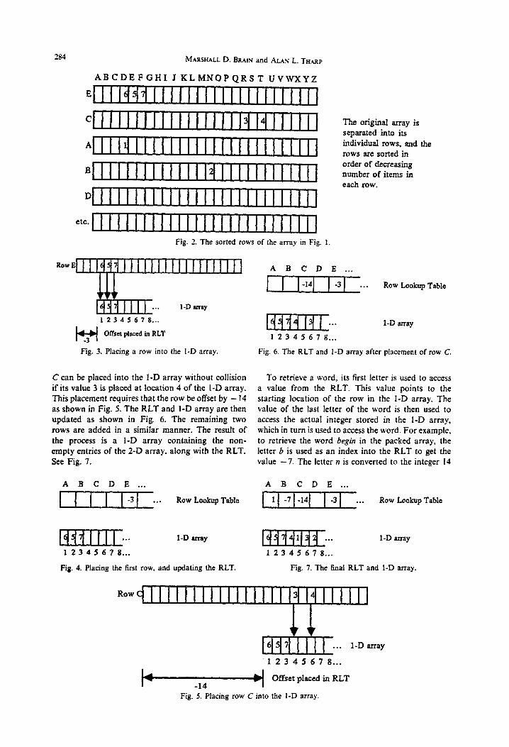
Figure 10 summarizes the operation of the algor- ithm by illustrating the packing of ail four rows from Fig. 1.

4. ANALYSIS OF THE SMP ALGORITH~I

Determining the computational complexity of the SMP algorithm is straightforward. Assume an r x r array contains r elements. Because the 2-D array contains r values, a minimally packed I-D array containing the contents of this 2-D array will also require r elements. In an r x r array containing r elements, each row will contain an average of one element. As each row is packed. every element in the row must be examined to determine if it collides with any existing values in the l-D array. Also. in the worst case, there are r possible positions for each row to occupy in the I-D array. Since each row can be considered to contain a single element, and since in the worst case r position for this row in the I-D array must be examined, r comparisons must be made. This same operation must be performed for all r rows in the 2-D array. Therefore, r’ comparisons must be performed to pack the 2-D array. The algorithm is O(r2) in the worst case.

To test the SMP algorithm, randomly filled sparse 2-D arrays of varying dimensions were packed using the algorithm. Table 1 summarizes the results of these tests. In the table, a 2-D array of the size indicated was sparsely filled with the number of values indi- cated in the number of entries coiumn. For example, for the 1000 x 1000 array size with 1000 entries stored in it, the 1000 values between I and 1000 were

A B C D E . . .

1 1 -7 j-141 1 -3) . . . Row Lookup Table

1 111 I 11 I I f f 8 I I .*. 1-D array

I2345678 . . . 15

Fig. 9. An example of non-minimal packing.

286 MARSHALL D. BRAIY and ALAN L. THARP

Row B llllllllllll~

h-4 Offset placed in RLT for Row B

Row A LLLI

Offset placed in RLT for Row A II

1

Row C llllllllllllllll] 3

-14 Offset placed in RLT for Row C

Row E I lpl,l,qJ 5

Offset placed in RLT for Row E ?

3 1-D array

1234567

A B C D E . . .

Row Lookup Table

Fig. IO. Packing the array in Fig. 1.

placed into raudomIy chosen locations in the array. The time required to pack the array was recorded. The array was then cleared and again randomly filled. Ten runs were performed for each test set shown in

Table 1. Performance characteristics of the SMP atgori&hm

Array Number of Average Average size entries time Is) I-D array size

26 x 26 34 0.137 34.900 ( i2.6%) 26 x 26 68 0.264 35.300 I+ 10.7%) 26 x 26 102 0.407 t20.500 f+is.l%) 26 x 26 136 0.571 169.200 (i 24.4%) 26 Y 26 170 0.736 23 I .7W ( + 36.3%) 26 x 26 204 0.912 295.500 (+44.9%) 26 x 26 272 I .297 436.600 f+bM%f

100x 100 100 0.330 fi2.100 (ilS.i%) 100x100 200 0.797 234.200 (+17.1%) 100 x 100 300 1.593 332.450 (f 10.8%) 100 x 100 400 2.374 447.400 (+11.8%) 100x100 500 3.143 572.COO (+ 14.4%) 100x loo 1000 8.901 1457.400 f +45.7%)

l000 x ~~0 50 0.225 3~.~ ( + 513.2%) 1000x1000 lo00 4.582 1234.700 ( + 23.5%) 1000 x ICIQO 2000 t 1.423 241 I.600 (+20.6%) 1000 x 1000 3000 79. ?20 3519.200 (+ 17.3%) 5000 x 5000 IO00 5.154 4713,700 (+371.4%) xJOox5000 2000 13.104 4918.000 (+ 145.9%) .5OoOx5wO 5000 50.319 6520.600 (+ 30.4%)

the table, and the average of the times and spaces were taken. The average times indicated were pro- duced using a PS/2 Model 70 using Turbo Pascal Version 5.0. The average 1-D array size column indicates the size of the I-D array once the 2-D array was packed into it. The percentages at the end of each line show the percentage of unused values in the I-D array. In ail cases, the size of the RLT is equivalent to the length of one row of the 2-D array (e.g. in a to00 x 1000 array, the RLT would contain 1000 integers-one integer for each row packed).

It may not he immediately obvious that 1000 x 1000 or 5000 x 5000 arrays have any appii- cation to perfect hashing. It will be shown that large arrays (e.g. 5000 x 5000) can he used for perfect hashing by using not just the first and last letter of the word to index the array, but instead using a function based on the first and last two or &fee letters of the word. For example, when the first and last pair of letters are used, 2-D arrays as large as 676 x 676 can be indexed.

Table 1 demonstrates several points about the SMP algorithm. First, the packing of the 2-D array down

Hashing using sparse matrix packing 287

123456 123456

0 3 I I I I -I Row L.ookup Table

1 2 3 4 5 6

1 6 5 4 2 3 1-D array

6

Fig. 1 I. Example 6 x 6 array to illustrate MSMP.

t Row 1 elements

h Row 2 elements

I Row 5 element

Fig. 13. The example 6 x 6 array packed with the MSMP algorithm.

to a I-D array with this algorithm generally does not produce minimal results. For example, when a 26 x 26 element array filled with 34 values is packed into a I-D array, on average 2.6% of the values in the I-D array are left unfilled. This non-mini~1 packing situation was shown in Figs 8 and 9. Table 1 also shows that the amount of unused space in the I-D table is related to the sparseness of the original 2-D array. Arrays that are extremely sparse (e.g. a 1000 x 1000 array containing 50 elements, or a 5000 x 5000 array containing 1000 elements) require more space when packed than do less sparse arrays. For example, if in the 5000 x 5000 array containing 1000 elements, one row has a value in both the first and the 5000th location, the 1-D array will require 5000 elements to hold the row, despite the fact that only lo00 elements will exist in the final 1-D array. Also, as the array fills with more and more elements, the space efficiency of the SMP algorithm fades. For example, packing 1000 elements filling a 100 x 100 array wastes space once packed. This waste occurs because as the number of items on each row increases, it becomes more difficult to pack the rows denseiy (it is much easier to densely pack rows that contain only one or two items). Tarjan and Yao [12] define a harmonic decay

model to describe this problem and provide a detailed explanation of the phenomenon.

the number of elements in the array is less than or equal to the number of rows in the array. This revised algorithm is called the minimal SMP algorithm

(MSMP algorithm). Instead of allowing values to be placed as far down as they would naturally fall in the 1-D array, the 1-D array is limited in size and out-of-bounds entries are moded back into that limited table size 1141.

The example 6 x 6 array in Fig. 1 I uses integer indexes for simplicity, but could just as easily be indexed using characters as shown in Fig. I.

Using the SMP algorithm, the 2-D array of Fig. 11 when stored into a 1-D array would be non-minimal as shown in Fig. 12. Location 4 in the 1-D array is unused, and therefore represents wasted space and non-minima1 packing. This problem can be solved by limiting the size of the 1-D array to 6 (the number of values being packed), and by adding a mod iunction to the hashing function:

hash-value = (row_lookup_table[ro~v_index]

f column-index) mod I-D-array-size

5. IMPROVING THE SMP ALGORITHM

The SMP algorithm can be modified slightly to produce minimally packed I-D arrays in cases where

By modifying the hashing function, the 1-D array and RLT would appear as shown in Fig. 13. For example, to locate the value in row 2, column 6, using Fig. 13, the value stored for row 2 in the RLT would be referenced. The value found at this position in the RLT is 3. This value in turn would be added to the column number desired (in this case 6) to obtain the value, 3 I- 6 = 9, which would then be moded by

123456

I I 0 I I Row Lookup Table

1 234567

- Row 1 elements The brackets show that

u Row 2 elements ~~~~~~~h~~~

I Row 5 element preserved.

Fig, 12. The example 6 x 6 array packed normally.

288 MARSHALL D. BRAIN and ALAN L. THARP

Table 2. Performance characteristics of the MSMP alnorithm

Array Number of Average Average size entries time (s) I-D array size

26 x 26 34 0.1 IO 34 (+o.o%) 26 x 26 68 I.294 76 (+ Ita%) 26 x 26 beyond 34 can’t pack minimally

100x loo 50 0.181 50 100 x 100 100 0.390 loo

ICO.O%1 ;+o.os/,;

100x 100 I30 0.527 120 (+O.O%) 100x100 140 0.698 140 (+o.o%) IO0 x IO0 beyond 140 can’t pack minimally

1~x1~ loo 0.412 IW (+0.0x) 1~x1~ IWO 5.885 IO00 (+o.o%) IGGox1ooo I300 24.934 1300 (iO.O%) WOO x IWO beyond 1300 can’t pack minimally 5000 x 5000 SOOOXSOOO :z

6.143 1000 (+o.o%) 30.549 2Mx) (+o.o%)

5000 x 5000 4000 145.132 4Ow (+o.o%) 5000x.5ooo 6000 340.897 6000 (+o.o%.) 5000 x 5000 beyond 6000 can’t pack minimallv

the I-D array size of 6 to obtain the result of 3. At location 3 in the I-D array is the value 5, as expected.

Table 2 shows the effect of this modification on packing time and space efficiency. Its column head- ings are the same as those for Table 1 and the runs to generate the data were performed in the same manner as for the SMP algorithm. It can be seen in Table 2 that as long as the number of elements remains approximately equaf to or less than the number of rows in the array, the array can be minimally packed. In terms of space, this outcome means that one integer (2 bytes) of storage (from the RLT) is needed to store a word with the MSMP algorithm when it is used for minimal perfect hashing. For example, if 5000 words are stored in a 5000 x 5000 array, the RLT will have 5000 entries (integers) in it, or 2 bytes per word being hashed.

The space requirements for the MSMP aigorithm at build time are Q(r). The row and column index plus the value of each element suffice to represent the 2-D array.

6. APPLICATION TO PERFECT HASHING

As has been shown, these algorithms can be easily used for perfect hashing. Minimal or non-minimal J-D arrays can be produced, depending upon whether time or space is more important. Words can be placed into a 26 x 26 element array, and the 2-D array can be packed down and later accessed by retaining only the 2delement RLT.

Unfortunately, the probability of finding a set of words that contain no pattern colksions under this algorithm decreases rapidly as the number of words increases, as it does for many other perfect hashing algorithms. For example, if the word list to be perfectly hashed in Fig. 1 had contained both been and begin, then a pattern collision would occur because both words start with a b and end with an n, and therefore map to the same location of the 2-D array. Table 3 shows the probability of pattern colJision vs the number of words being placed into a 26 x 26 element array. Knuth i15J calls this phenom-

Table 3. Probability of pattern collisions in a 26 x 26 array

Probability of collision

Number of words (%)

2 0.15 3 0.45

:8 7

26 30 50 40 71 50 85 60 93 70 97

enon the birrhduy paradox [2]. For example, the array in Fig. 1 contains 676 positions. If two random words are to be placed into the array, the probability of them not colliding at the same location is 675/676 = 99.85%. Therefore, the probability of col- lision is 0.15%. If three random words are placed in the array, then the probability of no collision decreses to (674~676) x (6751676) = 99.55%. Therefore, the probability of collision is 0.45%.

The pattern collision prob,tem occurs in many perfect hashing algorithms. For example, Sprugnoli 221 refers to the birthday paradox in his discussion of segmentation. Cichelli’s algorithm [4] cannot handle more than about 70 words (without resorting to segmentation) because of pattern collisions. Sager’s algorithm [S] is more immune to pattern collisions because of the increased complexity of the indexing functions used, but Sager shows that those pattern collisions that do arise must be handled by arbitrary manipulation of constants in the indexing functions.

One solution to the pattern collision problem in the aIgo~thms described in this article is to use, for exampfe, the first letter pair and the last letter pair (or the first and last tripfet, etc.) to increase the size of the 2-D array used to hash the words (it is also possible to use even more complicated techniques, as advo- cated by Sager [8J--any pair of functions can be used :o index into the 2-D array). Using letter pairs allows words to be placed into a 676 x 676 (26 x 26 = 676) array, which alJows perfect hashing of 200 words with only a 4.3% probability of a pattern collision. or 676 words with a pattern collision probability of 40%.

When using even Jarger lists, letter triplets can be employed. For example, to perfectIy hash 5000 words, the first and last tetter triplet can be used. This strategy produces an extremely Jarge 2-D array how- ever, since 26 x 26 x 26 = 17,576. To solve this prob- lem, mod functions can be used to reduce to size of the 2-D array. For example. if the first and last letter triplet’s values are moded by 5000, then the 2-D array size becomes 5000 x 5000.

7. COMPARISONS

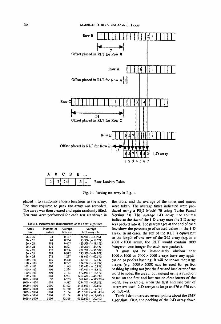
Table 4 compares the MSMP algorithm to other algorithms. The build order is the computational complexity of the algo~thm at build time. The I&t six

Hashing using sparse matrix packing ‘89

Algorithm

name

Table 4. Comparison of MSMP IO other perfect hashing algorithms

Build List CPU time

Reference order size (s) Machine

space

(bytes,

entry)

Cichelli

Karplus

Minicycle

FOX

Brain

MSMP

ISI

111

(111 -

6z

256

1000

1696

5000

35 IBM 4341 0.65

I50 Vax I I ,‘780 NA

45 IBM 4341 4.0

600 Mac II 4.0

733 PSi2/50 2.4

283 PSI2170 2.0

“Derived from experimental results.

is the example list size in the referenced article. The CPU rime is the time required to build the perfect hashing function for the word list on the machine specified in the machine column. The space column contains the number of bytes required (per item being hashed) to store the table needed to do retrieval using that perfect hashing function.

To create the entry for the MSMP algorithm in Table 4, a list of 5000 words (with three or more letters) containing no pattern collisions was chosen at random from the standard Unix word list (/usr/dict;words), and placed into a 5000 x 5000 element 2-D array. The two functions used as indexes to the 2-D array were:

row-index = (26 x 26 x (ord(s[length(s) - 1)))

+ (26 x ord(s[length(s) div 21))

+ ord(s[ 11)) mod array-size, (1)

column-index = (26 x 26 x ord(s[length(s)])

+ (26 x ord(s(length(s) - 21))

+ ord(s[length(s) - 31))

x mod array-size. (2)

The actual first and last letter triplets of the words are not used because letter triplets such as ing and con are common and cause non-uniform distribution of values in the 2-D array. Other indexing functions were also successfully used.

The words were minimally packed, using the MSMP algorithm, in 283 s of CPU time on an IBM PS/2 model 70. Because a 5000 x 5000 element 2-D array was used, the RLT contains 5000 integers-one word (2 bytes) of storage for each row in the list. For comparison, Cichelli’s algorithm uses a 26-value table (of bytes- for the 40 word list, or 0.65 bytes per word hashed. Sager [8] requires two words of 2 bytes each in the table formed for each item hashed.

In comparison to other current algorithms, the MSMP algorithm is superior both in terms of the CPU time required at build time and the storage required at retrieval time.

8. LIMITATIONS

The ability of the MSMP algorithm to form mini- mal perfect hashing functions has been tested on word lists containing up to 5000 words. To handle

5000 words, the indexing functions of equations (I) and (2) were used. When a 10,000 word list was attempted using these same indexing functions. mini- mal packing was not achieved. Analysis shah-ed the problem to involve a significant number of ro&s containing large numbers of entries. For example. if 10,000 values are randomly placed in a 10.000 x 10,000 array (as done to form the results in Tables 1 and 2), the row containing the most entries contains 10 filled elements. When actual words fill the 2-D array, however, many rows contain more than 50 elements when using the indexing functions of equations (1) and (2). This situation occurs because certain letter combinations are common in English words.

It is possible to improve the situation by using letter quadruplets, or by using more complicated indexing functions like those chosen by Sager [8]. The increased complexity of the indexing functions has the effect of distributing the words more evenly throughout the 2-D array. This solution may be impractical in some cases because it increases the amount of CPU time required for each retrieval.

As with other perfect hashing algorithms. the preferred solution for handling word lists of over 5000 words is segmentation of the word list. Segmen- tation also resolves pattern collision problems by placing colliding words into different segments. If space is not a factor, the SMP algorithm discussed can also be used to quickly produce non-minimal functions.

9. CONCLUSIONS

The MSMP algorithm can be used to replace other minimal perfect hashing algorithms, and has much better build time performance on extremely large word lists.

VI

121

[31

REFERENCES

E. A. Fox, Q. Chen, L. S. Heath and S. Dana. A more cost effective algorithm for finding minimal perfect hash functions. Proc. 1989 ACM CSC Cod. pp. 114-122 (1989). R. Sprugnoli. Perfect hashing functions: a single probe retrieving method for static sets. CACM 20( I I). 841-85071977). G. Jaeschke. Reciprocal hashing: a method for generat- ing minimal perfect hashing functions. CAC.bf 2*_0. 384-387 (1984).

290 MARSHALL D. BRAIN and ALAN L. THARP

[4] R. J. Cichelli. Minimal perfect hashing made simple. [IO] T. Lewis and C. Cook. Hashing for dynamic and static CACM 23(l). 17-19 (1980). internal tables. Compurer 45-56 (1988).

[5] K. Karplus and G. Haggard. Finding minimal perfect [I I] M. Brain and A. That-p. Near-perfect hashing of large hash functions. Proc. Serenreenth ACM SIGCSE word sets. Sofricare Practice Experience 19( IO), S,vmp. pp. 191-193 (1986). 967-978 (1989).

[6] K. Karplus and G. Haggard. Finding minimal perfect hash functions. Report TR84-637, Computer Science Dept Cornell University (1984).

[I21 R. E. Tarjan and A. C. Yao. Storing a sparse table. CACM22(11), 606-611 (1979).

[I31 M. L. Fredman and J. Komlos. Storing a sparse table with O(l) worst case access time. JdC.M l(3), 538-544 ( 1984).

[7] C. -C. Chang. The study of an ordered minimal oerfect hashing scheme. CACM 2714). 384-387 (1984).

[8] T. J. Sager. A-polynomial time generator for minimal perfect hash functions. CACM 28(S). 523-532 (1985).

[9] A. L. Tharp. File Organixiion and Processing. Wiley, New York (1988).

(141 T. Cook. Private Communication (1988). [15] D. E. Knuth. The Arr of Cornpurer Programming,

Vol. 3, p. 506. Addison-Wesley. Reading, Mass. (1973).