PERCEPTUAL SPEECH CONTROL

APPLICATION OF SPC IN PERCEPTUAL SPEECH QUALITY CONTROL

IN

MODERN MOBILE RADIO NETWORKS

This thesis is presented for the degree of Doctor of Philosophy

The University of Western Australia

School of Electrical, Electronic and Computer Engineering

August 2012

Ahmad Zamani Jusoh

B. S. Electronic Engineering

(Hanyang University, Republic of Korea)

M. Sc. Digital Communication Systems

(Loughborough University, UK)

THE UNIVERSITY OFWESTERN AUSTRALIA

DECLARATION FOR THESES CONTAINING PUBLISHED WORK AND/OR WORK PREPARED FORPUBLICATION

The exominotion of ihe thesis is on exominolion of the work of ihe student. The workmust hove been substonliolly conducted by the student during enrolmeni in lhedegree.

Where lhe thesis includes work lo which others hove contribuled, the thesis mustinclude o stotement lhot mokes lhe studenl's contribution cleor to the exominers. Thismoy be in the form of o descriplion of lhe precise contribution of lhe student io thework presenled for exominoiion ond/or o slotement of the percenloge of the work thotwos done by the student.

ln oddition, in ihe cose of co-outhored publicolions included in the thesis, eoch outhormust give their signed permission for lhe work to be included. lf signolures from oll lheouthors connol be obloined. the stotement detoiling the sludeni's conlribution to thework musl be signed by lhe coordinoling supervisor.

Pleose siqn one of lhe stotements below.

1. This ihesis does nol conloin work thot I hove published, nor work under review for publicotion

Student Signoture

2. This thesis contoins only sole-oulhored work, some of which hos been published ond/orprepored for publicotion under sole outhorship. The bibliogrophicol detoils of the work ond whereil oppeors in the lhesis ore outlined below.

Studenl Signoture

3. This lhesis contoins published work ond/or work prepored for publicoiion, some of which hosbeen co-qulhored. The bibliogrophicoldeioils of ihe work ond where il oppeors in the lhesis oreoutlined below.The student musi ottoch to this declorotion o stotement for eoch publicotion lhot clorifies thecontribulion of the student lo the work. This moy be in lhe form of o description of the preciseconlributions of lhe sludenl to the published work ond/or o stotement of percenl contribution bythe sludent. This siotemeni must be signed by ollouthors. lf signolures from otlthe oulhors connolbe obloined, the slotemenl detoiling lhe studenl's contribution lo the published work must besigned by the coordinoling supervisor.

A.Z. Jusoh, R. Togneri, B. Rohani, S. Nordholm, "CL\SUM Aoolication in Perceptual Sneech Oualitl,, Contol",Proceedines of APCC2009, October 2009, Shanghai, China, pp. 694-698.

Student Signoture

i

Abstract

One of the important aspects of a mobile communications industry is satisfying

customers’ needs most economically. Indeed, customers expect good and consistent

quality of service from the provider. As such, in mobile telephony, this amounts to

controlling speech quality as “perceived” by customers. Controlling perceptual speech

quality necessitates a reliable measurement of the quality first, followed by exercising

direct control over it.

The ultimate measure of perceived speech quality is realized through subjective

listening tests, but this is not practical for real-time day to day applications. In recent

years, objective quality measurement algorithms have been developed to predict the

subjective quality with considerable accuracy. And the ITU-T P.862 Perceptual

Evaluation of Speech Quality (PESQ) model is state of the art in the International

Telecommunication Union’s Telecommunication Standardization Sector (ITU-T)

recommendation for reference objective quality measurement method. However, these

algorithms have yet to be applied for end user quality control in cellular networks.

Hence, in this thesis, the research framework for application of the PESQ algorithm for

perceptual speech quality control is presented.

The PESQ algorithm has been extensively used in measurement tools for accurate

assessment of perceptual speech quality in modern telecommunication networks.

However, the smallest period that PESQ can evaluate speech quality is 320 ms. Even

though this or longer periods may be suitable for monitoring the speech quality, it may

be too long for effective control of quality in the network. PESQ is calculated based on

the so-called “Frame Disturbance” (FD) which is effectively the perceptual distance

between a reference and a distorted speech signal. The FD is calculated every 16 ms.

Even though 16 ms is too short for assessing speech quality but it is suitable for control

purposes. FD is investigated as a perceptual metric for control of speech quality in

modern networks replacing conventional metrics.

Since perceptual quality is a relatively long term aggregate of FD values, the

relationship between the statistics of FD values and the resulting speech quality needs to

be investigated. It is the outcome of this investigation which will help determine the

scheme most suitable for control of speech quality based on FD statistics. It is

ii

envisaged that the Statistical Process Control (SPC) which is a popular method in

manufacturing and industrial process control, will be a promising method.

The control of perceptual speech quality using mechanisms such as power control and a

“hybrid” control mechanism has been studied and applied before. However, a direct

control approach using controlling tools such as SPC will be the first to be attempted.

Statistical process control has been widely used in manufacturing and industrial quality

control. A statistical process control mechanism that has received much attention in the

statistical literature and usage in industry is the Cumulative Sum (CUSUM) method.

CUSUM detects process shifts faster than any other method. In this thesis, the

application of CUSUM in perceptual quality control based on FD in a Universal Mobile

Telecommunication Systems (UMTS) environment will be presented. Furthermore, the

performance of CUSUM will be compared with its counterpart in SPC: Exponential

Weighted Moving Average (EWMA). From these results, the CUSUM and EWMA

applications show better control in speech quality compared with the conventional

method used in UMTS.

iii

Table of Contents

Abstract ....................................................................................................................................... i

Table of Contents ...................................................................................................................... iii

Dedication ................................................................................................................................. vi

Acknowledgements .................................................................................................................. vii

List of Abbreviations................................................................................................................. ix

List of Common Symbols ......................................................................................................... xi

List of Figures ......................................................................................................................... xiii

List of Tables............................................................................................................................ xv

CHAPTER 1 ............................................................................................................................... 1

INTRODUCTION ....................................................................................................................... 1

1.1 Thesis structure ................................................................................................. 2

1.2 Summary of major Contributions...................................................................... 4

1.2.1 log (FDn) as the perceptual speech quality metric ........................................... 4

1.2.2 The CUSUM application in Speech Codec Rate and Power Control for

UMTS ........................................................................................................................ 4

1.2.3 The EWMA application in Power Control for UMTS ..................................... 5

1.3 Publications ....................................................................................................... 5

CHAPTER 2 ............................................................................................................................... 6

LITERATURE REVIEW ............................................................................................................. 6

2.0 Introduction ............................................................................................................. 6

2.1 Speech Quality Metrics and Measurement Method ................................................ 6

2.1.2 Perceptual Speech Quality Metric .................................................................... 8

2.2 Power Control Scheme.......................................................................................... 17

2.2.1 Centralized Power Control ............................................................................. 18

2.2.2 Distributed Power Control ............................................................................. 19

2.3 UMTS Power Control ........................................................................................... 20

2.3.1. Open Loop Power Control ............................................................................ 21

2.3.2. Closed Loop Power Control .......................................................................... 22

2.4 Statistical Process Control (SPC) .......................................................................... 27

2.5 Summary ............................................................................................................... 34

CHAPTER 3 ............................................................................................................................. 35

METHODOLOGY .................................................................................................................... 35

iv

3.0 Introduction ........................................................................................................... 35

3.1 Proposed Perceptual Speech Quality Control Model ............................................ 37

3.1.1 Motivation ...................................................................................................... 37

3.1.2 Proposed Model ............................................................................................. 37

3.1.3 Original Input Speech File and Speech Codec ................................................... 39

3.2 PESQ ..................................................................................................................... 40

3.2.1 Level Alignment ............................................................................................. 41

3.2.2 Input Filtering ................................................................................................. 41

3.2.3 Time Alignment and Equalization ................................................................. 41

3.2.4 Auditory Transform ....................................................................................... 41

3.2.5 Disturbance Processing and Cognitive Modelling ......................................... 42

3.2.6 Disturbance Aggregation and MOS Prediction .............................................. 42

3.2.7 Realignment of Bad Intervals ......................................................................... 43

3.3 Frame Disturbance ................................................................................................ 43

3.4 FQI Feedback Method .......................................................................................... 45

3.5 CUSUM ................................................................................................................ 47

3.5.1 Tabular CUSUM ............................................................................................ 48

3.5.2 The V-mask ........................................................................................................ 51

3.6 EWMA .................................................................................................................. 53

3.7 Closed Loop Power Control in FDD Mode .......................................................... 57

3.7.1 Conventional UMTS Outer Loop Power Control Algorithm ............................ 58

3.8 SPC Based UMTS Power Control ........................................................................ 60

3.9 Summary ............................................................................................................... 62

CHAPTER 4 ............................................................................................................................. 63

THE CUSUM TECHNIQUE APPLICATION IN PERCEPTUAL SPEECH QUALTY

CONTROL ................................................................................................................................ 63

4.0 Introduction ........................................................................................................... 63

4.1 Frame Disturbance Analysis ................................................................................. 64

4.1.2 Input speech file and speech codec ................................................................ 64

4.1.3 Methodology .................................................................................................. 64

4.1.4 Simulation result and discussion .................................................................... 65

4.2 Speech Codec Rate Control Simulation model ..................................................... 69

4.2.1 Introduction .................................................................................................... 69

4.2.2 Methodology .................................................................................................. 69

4.2.3 Simulation results and discussion .................................................................. 71

v

4.3 Power Control Simulation Model ......................................................................... 73

4.3.1 Input speech file ............................................................................................. 74

4.3.2 Speech codec .................................................................................................. 74

4.3.3 Multiplexing and channel coding ................................................................... 75

4.3.4 Power Control ................................................................................................ 76

4.3.5 Channel .......................................................................................................... 79

4.3.6 Summary of simulation parameters ............................................................... 80

4.3.7 Methodology .................................................................................................. 80

4.3.8. Simulation results and discussion ................................................................. 82

4.4 Summary ............................................................................................................... 94

CHAPTER 5 ............................................................................................................................. 96

THE EWMA TECNIQUE APPLICATION IN PERCEPTUAL SPEECH QUALITY CONTROL

.................................................................................................................................................. 96

5.0 Introduction ........................................................................................................... 96

5.1 Data Distributions Responses with the Application of EWMA and CUSUM ..... 97

5.1.1 Data Sample ................................................................................................... 97

5.1.2 Methodology .................................................................................................. 98

5.1.3 Simulation result and discussion .................................................................... 99

5.2 Power Control Simulation Model ....................................................................... 102

5.2.1 EWMA based UMTS Power Control .......................................................... 103

5.2.2 Summary of simulation parameters ............................................................. 105

5.2.3 Methodology ................................................................................................ 105

5.2.4. Simulation results and discussion ............................................................... 107

5.3 Summary ............................................................................................................. 125

CHAPTER 6 ........................................................................................................................... 126

CONCLUSIONS ..................................................................................................................... 126

6.1 Summary of Major Findings and Contributions ................................................. 127

6.2 Suggestions for Future Work .............................................................................. 129

APPENDIX ............................................................................................................................. 131

ITU Speech Files .................................................................................................................... 131

vi

Dedication

To my mother and my late father, Fatimah Che Long and Jusoh Latiff

vii

Acknowledgements

Thanks be to God!

Many people have helped me in the success of this project by supporting me with

different levels of assistance. I want to express my deepest gratitude, and would like to

thank them for their contributions

To my supervisory committee,

I would like to sincerely thank my wonderful supervisors, Associate Professor Roberto

Togneri and Professor Sven Nordholm, for sharing their knowledge and giving me such

helpful guidance along the way to completing this thesis. Their advice and comments

have been insightful to me. Not forgetting a special thanks to my former supervisor, Dr

Bijan Rohani for initiating this research and giving me ideas to enhance it.

To the UWA staff members,

I wish to express appreciation to all of those people who assisted me in performing my

experimental work, also my PhD documentation. My thanks to my lab mates, Sarajul,

Daniel, and Ingrid who assisted and shared the experience in doing the research.

To my colleagues and friends,

A special thanks to my friend, Daniel for willingly being my proof reader. I really

appreciated it. To all my friends who made me enjoy living in Perth and giving me

support during my hard work doing PhD, Nurazura Mohd Diah, Nor Azlin Tajuddin,

Ibrahim Abdul Rahman, Nadzril Sulaiman, Ahmad Fareed Ismail, Hamdan Daniyal,

Nor Fadhilah Mohd Azmin, Abdul Malek Abdul Hamid and etc.

To my family,

Thanks to my mother, Fatimah Che Long, my late father, Jusoh Latiff, my lovely wife,

Nor Haslinda Abdul Hameed, my sisters: Zamilah, Zaiton, Zarini and Zahariayana, my

viii

brothers: Mohd Zainuddin, Mohd Zakuan and Mohd Zaim Rasyidi, my family in law,

Bungsu Ismail and Mohd Yusof Mohd Nor & family for always being with me in bad

and good moments. Thanks for your prayers, patience, love and moral guidance

throughout my critical time. Their tremendous support has succeeded in assisting me to

complete this thesis.

Last but not least, a special thanks to my employer, International Islamic University

Malaysia and Ministry of Higher Education for giving me the opportunity and

scholarship in making my PhD journey a reality

ix

List of Abbreviations

3G Third Generation

3SQM Single Sided Speech Quality Measure

ACR Absolute Category Rating

ACELP Algebraic Code Excited Linear Prediction

AMR Adaptive Multi-Rate

ANIQUE Audio Non-intrusive Quality Estimation

ARL Average Run Length

ASD Auditory Spectrum Distance

BER Bit Error Rate

BS Base Station

BSD Bark Spectral Distance

BTS Base transceiver Station

CC Convolutional Coding

CD Cepstral Distance

CDMA Code Division Multiple Access

CePC Centralized Power Control Scheme

CLPC Closed Loop Power Control

CRC Cyclic Redundancy Check

CUSUM Cumulative Sum

DCR Degradation Category Rating

DMOS Degradation Mean Opinion Score

DPC Distributed Power Control

EWMA Exponentially Weighted Moving Average

ETSI European Telecommunications Standards Institute

FDD Frequency Division Duplex

FDMA Frequency Division Multiple Access

FER Frame Error Rate

FEP Frame Erasure Pattern

FD Frame Disturbance

FQI Frame Quality Indicator

FTT Fast Fourier Transform

GMA Geometric Moving Average

IRS Intermediate Reference System

x

ITU International Telecommunication Union

ITU-T International Telecommunication Union Telecommunication

Standardization Sector

MNB Measuring Normalizing Blocks

MS Mobile Station

MOS Mean Opinion Score

OLPC Open Loop Power Control

OPCS Optimum Power Control Scheme

PAMS Perceptual Analysis Measurement System

PCM Pulse Code Modulation

PAQM Perceptual Audio Quality Measure

PESQ Perceptual Evaluation Speech Quality

PSD Power Spectral Density

PSQM Perceptual Speech Quality Measure

QoS Quality of Service

RNC Radio Network Controller

SIR Signal Interference Ratio

SPC Statistical Process Control

TDD Time Division Duplex

TDMA Time Division Multiple Access

TPC Transmit Power Control

TSPC Target-SIR-tracking Power Control

UE User Equipment

UMTS Universal Mobile Telecommunication System

TQM Total Quality Management

VoIP Voice over Internet Protocol

xi

List of Common Symbols

R Transmission rating of E-model

TPCcm TPC command

δ Step size in inner loop power control

rxTPCcmd Received TPC command

txTPCcmd Transmitted TPC command

X - chart Shewhart Sample Mean

R-chart Shewhart Sample Range

p-chart Sample Proportion Defective

np-chart Sample Number of Defectives

c-chart Sample Number of Defects

u-chart or c -chart Sample Number of defects per unit

( )nD f Disturbance density

( )nDA f Asymmetrical disturbance density

N Frame number

nM Multiplication factor

Nb Number of bark band

fW Series of constants

0µ Target value of CUSUM

C+ Upper limit of CUSUM

C− Lower limit of CUSUM

K Reference value of CUSUM

H Tabular CUSUM limit

σ Standard deviation

0C + Initial CUSUM

0C − Initial CUSUM

α Probability of a false alarm in CUSUM

β Probability of not detecting a shift of the size δ

L Width of the EWMA control limits factor

1z First value of EWMA

UCL Upper control limit of EWMA

xii

LCL Lower control limit of EWMA

sµ Estimated mean log(FD)

∆ Step size in outer loop power control

P Statistical significant value

l Slot index for inner loop power control algorithm

xiii

List of Figures

2.1 Speech quality metric categorization……………………...………….... 7

2.2 Speech quality metrics and location measured………….……………... 7

2.3 Anatomy of the human ear………...…………………………………… 9

2.4 Basic operations performed by a perceptual speech quality metric…… 13

2.5 UMTS power control basic block diagram……………………………. 21

2.6 Open Loop Power Control operation………………………………..… 22

2.7 Closed Loop Power Control operation………………………………… 23

2.8 Block diagram of UMTS CLPC…….…………………………………. 23

2.9 General outer loop power control algorithm…………………………... 24

2.10 General inner loop power control algorithm…………………………... 25

2.11 Production process inputs and outputs………………………………… 28

2.12 Sample of Histogram………………………………………….……….. 29

2.13 Sample of Pareto Chart………………………………………………… 30

2.14 Sample of Cause and Effects Diagram………………………………… 30

2.15 Sample of Scatter Diagram……………………………………………. 31

2.16 Process improvement using the Control Chart………………………… 32

2.17 Sample of basic Shewhart Control Chart………………………………. 33

3.1 Example of perceptual speech quality experienced by more than 30

end users in a simulated 3G UMTS network…………………………...

36

3.2 Proposed model for speech codec rate control………………………… 38

3.3 Application of CUSUM/EWMA based on nFD ..………………………... 38

3.4 PESQ block diagram…………………………………………...……… 40

3.5 Structure of PESQ model…………………………………...…………. 40

3.6 nFD concept in controlling perceptual quality………………………… 44

3.7 The classification of the encoded speech bits and their unequal error

protection scheme for UMTS…………………………………….…….

45

3.8 Block diagram of FQI feedback method………...…………………….. 46

3.9 Sample of Tabular CUSUM………………………………...…………. 50

3.10 A typical V-Mask…………………………….………………………... 51

3.11 The physical distance between subgroup samples is equivalent to a

unit on the vertical axis………………………………………………....

52

3.12 Sample of EWMA chart…...……………………………….………….. 55

xiv

3.13 Conventional UMTS outer-loop power control flow chart……………. 59

3.14 SPC based UMTS outer-loop power control………………..…………. 61

4.1 Simulation model for frame disturbance analysis………........................ 65

4.2 log( )nFD distribution for PESQ MOS 3.0-3.5: (a) 3.0, (b) 3.1, (c) 3.2,

(d) 3.3, (e) 3.4 and (f) 3.5…………………………………….................

68 4.3 The simulation model for speech codec rate control…………………... 69

4.4 A CUSUM control chart without the controlling speech codec rate…... 71

4.5 Apply CUSUM with controlling speech codec rate…………………... 71

4.6 A CUSUM control chart without the controlling speech codec rate…... 72

4.7 Apply CUSUM with controlling speech codec rate…………………… 73

4.8 Block diagram of the simulation model of UMTS physical layer (FDD

mode)…………………………………………………………………...

74

4.9 Application of CUSUM in UMTS outer-loop power control…...…….. 77

4.10 CUSUM based UMTS outer-loop power control……………….…….. 78

4.11 Performance comparison of CUSUM based and conventional power

control (shadowing profile 5 and ∆ = 0.005 dB): (a) 3 km h-1 ,

(b) 50 km h-1 and (c) 120 km h-1………………………………………..

91

4.12 Performance comparison of CUSUM based and conventional power

control (shadowing profile 1 and ∆ = 0.02 dB): (a) 3 km h-1 ,

(b) 50 km h-1 and (c) 120 km h-1………………………………………..

93

5.1 Data sample which has a normal distribution…………………...……... 97

5.2 Data sample which not has a normal distribution…………………...…. 98

5.3 Result of the application of (a) EWMA technique and (b) CUSUM

technique to the normal distribution data………………........................

100

5.4 Result of the application of (a) EWMA technique and (b) CUSUM

technique to the non-normal distribution data………………………….

101

5.5 Application of EWMA in UMTS outer-loop power control…………... 103

5.6 EWMA based UMTS outer-loop power control………………………. 104

5.7 Performance comparison of conventional, CUSUM based and EWMA

based power control (shadowing profile 5 and ∆ = 0.005 dB):

(a) 3 km h-1 , (b) 50 km h-1 and (c) 120 km h-1………………………...

121

5.8 Performance comparison of conventional, CUSUM based and EWMA

based power control (shadowing profile 1 and ∆ = 0.01 dB):

(a) 3 km h-1 , (b) 50 km h-1 and (c) 120 km h-1………………………...

124

xv

List of Tables

3.1 Number of bits in Classes A, B, and C for each AMR codec mode……… 39

3.2 The parameters of for the sample of Tabular CUSUM chart……………... 49

3.3 EWMA parameters for the sample of EWMA chart……………………... 55

4.1 The estimated mean, 0

µ and the standard deviation of log( )nFD

distribution…………………………………………………………………

68

4.2 Parameters chosen for CUSUM chart ……….…………………………… 70

4.3 Summary of AMR codec mode 7 frame structure………………………... 75

4.4 Conventional UMTS power control

parameters…………………………...

77

4.5 Tapped-delay-line parameters for Vehicular A environment…………..…. 79

4.6 Main simulation parameters………………………………………...…….. 81

4.7 Results for conventional and CUSUM based power control algorithms

with outer-loop step down, ∆down = 0.005 dB and vehicular speed of

(a) 3 km h-1, (b) 50 km h-1 and (c) 120 km h-1……………………………..

84



(a) 3 km h-1, (b) 50 km h-1 and (c) 120 km h-1…………………..................

85



(a) 3 km h-1, (b) 50 km h-1 and (c) 120 km h-1…………………..................

86



(a) 3 km h-1, (b) 50 km h-1 and (c) 120 km h-1…………………………… .

87

4.11

Results for conventional and CUSUM based power control algorithms for

all outer-loop step sizes and vehicular speed of (a) 3 km h-1, (b) 50 km h-1

and (c) 120 km h-1…………………………………………………………

88

5.1 Chosen parameters for normal distribution data: (a) EWMA and

(b) CUSUM………………………………………………………………..

99

5.2 Chosen parameters for the non-normal distribution data: (a) EWMA and

(b) CUSUM………………………………………………………………..

99

5.3 Main Simulation Parameters………………………………………………

106

xvi

5.4 Results for Conventional and EWMA based power control algorithms


(a) 3 km h-1, (b) 50 km h-1 and (c) 120 km h-1……………………………

108




109




110




111

5.8 Results for EWMA and CUSUM based power control algorithms with

outer-loop step down, ∆down = 0.005 dB and vehicular speed of


112


outer-loop step down,, ∆down = 0.01 dB and vehicular speed of

(a) 3 km h-1, (b) 50 km h-1 and (c) 120 km h-1…………………………….

113



(a) 3 km h-1, (b) 50 km h-1 and (c) 120 km h-1…………………………..…

114




115

5.12

Result for Conventional and CUSUM based power control algorithms for

all simulated outer loop step sizes and vehicular speed of


116

5.13

Result for EWMA and CUSUM based power control algorithms for all

simulated outer loop step sizes and vehicular speed of


117

xvii

A ITU Speech files used for FD analysis for PESQ MOS 3.0………………. 131

B ITU Speech files used for FD analysis for PESQ MOS 3.1………………. 131

C ITU Speech files used for FD analysis for PESQ MOS 3.2………………. 131

D ITU Speech files used for FD analysis for PESQ MOS 3.3………………. 132

E ITU Speech files used for FD analysis for PESQ MOS 3.4………………. 132

F ITU Speech files used for FD analysis for PESQ MOS 3.5………………. 132

1

CHAPTER 1

INTRODUCTION

As a result of increasing competition, measurement and control of the end-user

perception of service quality are becoming increasingly important to cellular network

operators. To measure and control perceptual speech quality efficiently, an accurate

speech quality measurement is required. In many modern cellular networks, accurate

speech quality measurements are required for a variety of reasons. These range from

daily network maintenance to radio resource management through power control and

link adaptation.

To date, speech quality has been monitored and controlled based on

conventional measurements such as Signal Interference Ratio (SIR), Bit Error Rate

(BER), and Frame Error Rate (FER). FER measure is widely used in systems such as

3G UMTS (Universal Mobile Telecommunication System) because it is recognised as a

good measure of speech quality. However, FER is not a perceptual measure of speech

quality. Furthermore, none of these non-perceptual measurements have been shown to

estimate speech quality with sufficient accuracy or reliability [1].

However, these parametric methods with their inferior performance are still

commonly used. Since these methods lack accuracy in their prediction of perceived

speech quality, the service provider needs to cater for the worst case scenario in order to

ensure that the quality expectations of almost all customers are met; that is, the provider

will have to unnecessarily expend more resources, such as transmission power and

speech codec rate to prevent speech quality from dropping below a certain acceptable

limit. There are no constraints on the upper quality value. Therefore, often more than

adequate quality is provided at the expense of valuable resources. That is, the available

methods do not control the perceptual quality directly, but they do so indirectly through

some relevant channel measures. Furthermore, applying any control on the signal will

only result in corresponding changes in the variables measured by the parametric

method, i.e. FER, SIR or BER.

A truly perceptual quality measure is obtained when we analyse the received

speech signal with a perceptual algorithm Perceptual Evaluation of Speech Quality

(PESQ) model which is a state of the art International Telecommunication Union’s

Telecommunication Standardization sector (ITU-T) recommendation for referenced

perceptual model measurement methods. PESQ has been designed to improve on the

2

previous objective methods. It is implemented commercially in testing devices and

monitoring systems [2]. As such, the application of PESQ as a monitoring and

controlling method will be beneficial to the telecommunications industry. In this thesis,

the speech quality monitor and control based on Frame Disturbance (FD) which is

subtracted from a PESQ algorithm will be investigated. The Frame Quality Indicator

(FQI) method used for estimation of the perceptual speech quality is applied in this

research application to ensure the employment of FD statistical data as speech quality

metric is possible.

The main aim of this research is to first incorporate perceptual based quality

measurement schemes to replace their traditional counterparts in mobile networks.

Subsequently, methods for direct control of the perceptual speech quality such as

Statistical Process Control (SPC) are applied in mobile communication systems. The

control of perceptual speech quality using mechanisms such as power control and

“hybrid” control mechanism has been studied and applied before [3-5], however, direct

control approach using controlling tools such as SPC is the first attempted.

Statistical process control has been widely used in manufacturing and industrial

quality control [6]. A statistical process control mechanism that has received much

attention in the statistic literature and usage in industry in controlling the process mean

is the Cumulative Sum (CUSUM) method. Furthermore, the CUSUM scheme detects

process shifts faster than any other method [7]. Hence, in this thesis a direct control

approach using the CUSUM scheme to control the perceptual speech quality will be

analysed. The performance of the scheme is compared to its counterpart tool in SPC,

Exponentially Weighted Moving Average (EWMA) scheme.

The outcome of this study is that it potentially benefits both the network

provider and users. The provider can optimize the network resources by providing just

enough resources to meet required levels of service as well as providing consistent

perceived quality to the customers. This is achieved while maintaining a satisfactory

service level for all customers.

1.1 Thesis structure

Chapter 2 covered the literature review for the thesis. The chapter starts with the survey

of speech quality metrics. The power control schemes used in mobile communication

systems is then described and discussed. The SPC and its tool are reviewed at end of the

chapter.

3

In Chapter 3, a novel method of controlling power as well as the speech codec

rate is proposed, both of which are associated with the usage of power in mobile

communication systems. PESQ, state of the art for referenced perceptual speech quality

measure is explored in the proposed system. FD which is subtracted from PESQ and is

proposed to replace the non-perceptual speech quality metric such as FER is described

in detail in the chapter. The FQI method used for estimation of perceptual speech

quality in this research application is also discussed. The direct control approach using

SPC tools - CUSUM and EWMA, which has not yet been explored in mobile

communications systems, is described in detail at end of the chapter.

In Chapter 4, the speech codec rate and power control using a CUSUM based

technique is applied in UMTS to improve the performance of UMTS. The chapter

begins with the analysis of the FD which is subtracted from PESQ. As a result, it shows

that log( )nFD possesses a normal distribution. Since CUSUM is naturally applied to the

normal distribution data, the employment of CUSUM in this research is justified. Then,

the application and analysis of the CUSUM based technique for controlling the speech

codec rate and power control in UMTS are discussed. It shows how fast the new

proposed perceptual speech quality metric, log( )nFD incorporates with CUSUM to

control the speech quality. Here, the CUSUM based power control algorithm

performance is compared with that of the UMTS conventional power control algorithm.

It is demonstrated that CUSUM based power control achieves adequate speech quality

while using less system resources. The application of a CUSUM based technique in

power control for UMTS, shows that the technique has up to a 13% reduction in the

average SIR target compared to the conventional counterpart.

In Chapter 5, power control using the EWMA based technique is applied in

UMTS to compare with the CUSUM based technique. The chapter begins with the

response of data distributions (normal and non-normal distribution) to the application of

both techniques. It shows that, in a particular study, EWMA is more superior in

detecting the shift for the non-normal data distribution than the CUSUM technique. The

application and analysis of the EWMA based technique for controlling the power

control for UMTS performance is compared to the conventional CUSUM based

technique. The result shows, CUSUM based technique achieves up to 5% reduction in

the SIR target compared to the EWMA based technique. However, the EWMA based

technique achieves up to 9% reduction in the SIR target compared to the conventional

based technique.

4

1.2 Summary of major Contributions

In this section, the major contributions of the thesis are summarized. These

contributions, to the best of the author’s knowledge, are innovative and have not been

published previously by other authors.

1.2.1 log (FDn) as the perceptual speech quality metric

The PESQ algorithm has been extensively used in measurement tools for accurate

assessment of perceptual speech quality in modern telecommunication networks.

However, the smallest period that PESQ can evaluate speech quality is 320 ms [8].

Even though this or longer periods may be suitable for monitoring speech quality, it

may be too long for effective control of quality in the network. As such, it will be

necessary to investigate metrics which can be calculated faster than 320 ms for

application in controlling the quality.

The PESQ is calculated based on the so-called “Frame Disturbance”, (FD) which is

effectively the perceptual distance between the reference and the distorted speech

signals [9]. The FD is calculated every 16 ms. Even though 16 ms is too short for

assessing speech quality it is suitable for control purposes . It is proposed that the FD is

investigated as a perceptual metric for control of speech quality in modern networks.

Since the perceptual quality is a relatively long term aggregate of the FD values

[2], the relationship between the statistics of FD values and the resulting speech quality

is investigated and the numerical analysis of the FD shows that log( )nFD has a normal

distribution for a given perceptual quality, the Mean Opinion Score (MOS). It also

demonstrated that the mean of distributions of log( )nFD is increased with the

degradation of the perceptual quality and vice versa. The result of the FD statistics data

shows it is applicable and appropriate for the application of SPC schemes in directly

controlling the perceptual speech quality.

1.2.2 The CUSUM application in Speech Codec Rate and Power Control for UMTS

The application of CUSUM based speech codec rate control for UMTS. CUSUM based

technique allows faster action at the transmitter to control the quality of the speech

signals as required by end users. The performance is compared between CUSUM based

5

and FER based outer loop power control algorithms through simulations. It is revealed

that the CUSUM based power control achieves adequate speech quality while reducing

the average SIR target by up to 13% relative to the conventional algorithm.

1.2.3 The EWMA application in Power Control for UMTS

The analysis between EWMA and CUSUM techniques control with normal distribution

data and non-normal distribution data is compared. It shows that in our case, a EWMA

technique has a better response with the data which does not have a normal distribution

compared to the CUSUM technique. A EWMA based technique is also superior in

detecting the larger shift than a CUSUM based technique. However, on the other hand,

a CUSUM technique has a better response with the normal distribution data compared

to the EWMA technique.

A EWMA based power control technique is applied for UMTS to compare with

the performance of conventional and CUSUM based power control techniques. It is

shown that both EWMA and CUSUM algorithms reduce the average SIR target

compared to a conventional algorithm. However, the CUSUM based power control

achieves adequate speech quality while reducing the average SIR target slightly by up to

5% relative to the EWMA based algorithm.

1.3 Publications

The following publication corroborates the material presented in this thesis:

1. Jusoh A.Z., Togneri R., Rohani B., and Nordholm S, " CUSUM application in

perceptual speech quality control, in 15th Asia-Pasific Conference on

Communication (APCC 2009), Shanghai, China, October 2009, pp694-698.

6

CHAPTER 2

LITERATURE REVIEW

2.0 Introduction Nowadays, the demand for mobile communications is increasing rapidly as well as its

featured technology. However, speech communication is still the main requirement by

end users. The service provider’s profit is dependent on the service provided.

Nevertheless, the demand for the service is dependent on the end user’s satisfaction

from the Quality of Service (QoS) they receive. Therefore, in mobile telephony, this

amounts to controlling speech quality as “perceived” by customers. Controlling

perceptual speech quality necessitates a reliable measurement of the quality first,

followed by exercising direct control of it. Power control schemes have been proposed

to increase the optimization of the resources as well as providing a better quality of

service to mobile network customers [10]. SPC has been widely used in manufacturing

and industrial quality control [6]. However, a direct control approach using SPC has not

yet been explored in mobile communications systems. In this chapter, the survey of

speech quality metrics, followed by the review of power control schemes of mobile

radio systems and SPC, is presented.

2.1 Speech Quality Metrics and Measurement Method

There is a wide range of metrics used, and could be used, to assess speech quality in

mobile radio networks. Figure 2.1 shows the range of the metric used from the

conventional metric to the perceptual metric. There are two types of perceptual metric:

objective and subjective. Furthermore, under objective perceptual metrics, there are the

referenced and non-referenced metrics.

7

Figure 2.1: Speech quality metrics categorization.

Traditionally, the speech quality in wireless systems is estimated based on parametric

methods that rely on channel quality measurements at the receiver [4, 11, 12] SIR, BER,

and FER are the more widely used metrics in mobile radio systems.

Figure 2.2: Speech quality metrics and location measured.

Figure 2.2 shows the speech quality metrics and where they are measured in

simplified communication systems. The simplest quality measure at the receiver side is

SIR. It is the quotient between the average received modulated carrier power S or C and

the average received co-channel interference power I. SIR is directly related to the

Speech Encoder

Channel Decoder Demodulator

Modulator Channel Encoder

Speech Decoder

Speech In

Reconstructed Speech Out

Channel

Perceptual Speech Quality Metric

FER BER SIR

Transmitter

Receiver

Speech Quality Metric

Conventional Perceptual

Subjective

Referenced

Objective

Non-referenced

8

carrier hence easy to be controlled. The BER can be measured after demodulation. BER

is defined as the average number of bits that are in error as compared with the total bits

entering the modulator over a given period of time. And, FER can be measured after the

speech undergoes the channel decoding process. FER can be defined as the ratio of

frames which are in error, to the total number of frames over the given period of time.

All of these measurements are related to speech quality. Among them, FER is

considered to be the most reliable and commonly used in modern mobile radio

networks, since frame errors are the major cause for quality degradation in speech signal

quality. However none of these measurements have been shown to accurately and

reliably estimate speech quality [1].

However, these parametric methods, with their poor performance in measuring

the true speech quality, are still commonly used. Since these methods lack accuracy in

their prediction of perceived speech quality, the service provider needs to cater for the

worst case scenario in order to ensure that the quality expectations of almost all the

customers are met; that is, the provider will have to unnecessarily expend more

resources, such as transmission power and speech codec rate to prevent speech quality

from dropping below a certain acceptable limit. There are no constraints on the upper

quality value. Therefore, often more than adequate quality is provided at the expense of

valuable resources. That is, the available methods do not control perceptual quality

directly but they do so indirectly through some relevant channel measures.

2.1.2 Perceptual Speech Quality Metric A truly perceptual quality measure is obtained when we analyse the received speech

signal with a perceptual algorithm based on the human hearing system. Perceptual

speech quality measurement is relatively new to mobile radio networks. Perceptual

speech quality measure is based on a psychoacoustics sound representation which will

be elaborated on in detail in the following sections. There are two types of perceptual

measurement methods: subjective and objective [13]. The subjective method uses a

human as a test subject, while the contrary objective method uses a model instead of a

human. Due to drawbacks of the subjective method such as being expensive, time

consuming and not suitable for day-to-day application [13-15], the objective method is

more appropriately applied in this research.

9

Psychoacoustics Psychoacoustics is the study of human perception of sound [16]. Sound is an alternating

air pressure which emanates from the source through a medium to the receptor. The

human perception of sound depends on the auditory behavioural responses of human

listeners, the abilities and limitations of the human ear, and the auditory complex

process which occurs inside the brain.

Figure 2.3: Anatomy of the human ear [17].

The human ear is divided into three parts: the outer ear, middle ear and the inner

ear as illustrated in Figure 2.3. The outer ear amplifies the incoming air vibrations. The

middle ear transduces these into mechanical vibrations and the inner ear filters and

converts them into hydrodynamic and electro-mechanical vibrations, after which, those

electromechanical signals are transmitted through nerves to the brain.

The human auditory system is remarkable in terms of absolute sensitivity and

the range of intensities to which it can respond [16]. Intensity means the acoustic power

of a sound per unit of area. The audible frequency of the human ear is roughly between

20 and 20,000 Hz and its intensity can be up to 120 dB. Human hearing has a binaural

hearing characteristic that allows humans to localize the sound by registering slight

differences in time, phase, and intensity of sound striking each ear. Human hearing also

can detect time differences as slight as 30 ms, which automatically compares the left

and right ear receptions and evaluates the sound’s intensity so that it allows humans to

identify the approximate location of the original sound.

Sound may be generally characterized by pitch, loudness, and timbre. In

psychoacoustics, pitch is the psychological perception of frequency. From the research

undertaken such as in [18] , pitch is a response pattern to the frequency of a sound. In

10

music, it is defined as the position of a single sound in the complete range of sound

from lowest to highest. The rise and fall in pitch is dependent on the strength of

vibration of the sound waves that produce that particular sound.

Loudness is a subjective perception of the intensity of sound. The ear is less

sensitive to low frequencies. The maximum sensitivity of human hearing is between

1,000 and 5,000 Hz and the standard threshold of hearing at 1,000 Hz is nominally

taken to be 0 dB.

Timbre is the ability of the ear to distinguish two similar sounds that have the

same pitch and loudness. It is mainly determined by harmonic content and dynamic

characteristics that allow us to discriminate sounds produced by the different sources we

hear at the same time.

The concept of critical bands, masking phenomena and the minimum threshold

of hearing of the human auditory system are important in psychoacoustic modelling

[19]. A critical band is the smallest band of frequencies that activate the same part of the

basilar membrane at the cochlea at the inner ear. The concept of critical bands was

introduced by Fletcher in 1940 [20] and has been widely tested. J.V. Tobias revealed the

critical band scale in 1970 [21]. From that scale, it is clear that the critical bands are

much narrower at low frequencies than at high frequencies where ¾ of the critical bands

are below 5,000 Hz. At low frequencies the ear can distinguish tones of a few hertz

difference but at high frequencies tones must differ by hundreds of Hertz to be

distinguished. When two sounds with equal loudness when sounded separately are close

together in pitch, their combined loudness when sounded together will be only slightly

louder than one of them alone. They might be in the same critical band where they are

competing against each other for the same nerve endings on the basilar membrane of the

inner ear. If the two sounds have a wide difference of pitch, the perceived loudness of

the combined tones will be greater because they do not overlap on the basilar membrane

and compete for the same hair cells. And, if the tones are not in the critical bands, the

combination of both can be perceived twice as loudly as one alone. The theory of

critical band shows that the human auditory system can discriminate energy use

between inside and outside bands.

Simultaneous masking is a characteristic of the human auditory systems where

some sounds fade away in the presence of louder sounds [22]. The louder sound is

called masker and the softer sound is called maskee. Instantaneous masking was

essentially defined through experimentation with pure tones and narrow-band noises

[20, 23]. Masking is the most powerful characteristic of modern lossy coders. The

11

sound signals which are going to be coded are compared to the minimum threshold and

masking curve. If the sound signals fall below the threshold, they will be discarded

since the ear cannot hear them.

A coder for a communication system based on critical band and masking in an

auditory system has been explored. For example, in 1980, Michael A. Krasner [24]

developed a multiband speech encoding system which uses the results of

psychoacoustic experiments to specify the system structure and parameters.

Subjective Speech Quality Measure The International Telecommunication Union (ITU) P.800 Recommendation [25]

describes several methods and procedures for subjective evaluations of transmission

quality. The most commonly used method is the Absolute Category Rating (ACR) and

Degradation Category Rating (DCR) tests. Subjective tests are normally carried out

under controlled conditions in the laboratory. The subjective perceptual measurement

method involves a group of participants rating the quality of some speech samples in a

strictly controlled environment. Careful test design can control some undesirable factors

that influence the voting process.

For an ACR listening test, subjects, (untrained listeners), have to rate the overall

quality of a speech clip which may have distortion without comparing it with the

original speech clip. This means the subjects do not have to refer to the original speech

clip in rating the given speech clip. The listeners have to give each sentence a rating

from 1 to 5 as follows: (1) bad; (2) poor; (3) fair; (4) good; (5) excellent. The

arithmetical mean of all the individual scores is the MOS and represents the overall

subjective rating of the speech sample [7].

For a DCR test, the listeners have to rate the degradation level of the speech by

comparing the speech clip under test to the original clip. The listeners have to give each

sentence a rating from 1 to 5 as follows: (1) very annoying; (2) annoying; (3) slightly

annoying; (4) audible but not annoying; (5) inaudible. The average of the opinion scores

of subjects in DCR is called the Degradation Mean Opinion Score (DMOS). The DCR

test provides more sensitivity in speech quality evaluation than the ACR method since

the reference speech is provided particularly when evaluating the good quality speech.

The ACR test tends to be insensitive to the extent that small differences in quality are

not detected.

Subjective testing methods have been developed to provide an overall score of

the quality of a system or service from the customer’s viewpoint, independent of the

12

underlying technology used in the network. This method is widely used in

communication systems even though it has limitations. For example, in subjective

perceptual measure, the definition of the test condition and the interpretation of results

are crucial. Hence, this method is tedious, error-prone, expensive, time consuming and

not suitable for real-time and day-to-day application [13-15]. Furthermore the tests and

the results of this method are not always reproducible. However, the subjective

perceptual measures are important because they are the ultimate measure of quality and

provide a benchmark for evaluation and comparison among other speech quality

measures.

Objective Speech Quality Measure In order to avoid the undesirable features of subjective tests, objective perceptual

methods have been invented. By contrast with the subjective perceptual measure,

objective perceptual measure replaces the human subject with a computer model.

Objective perceptual methods use models based on the human auditory system

properties in an attempt to derive quality estimations which are close to the subjective

perceptual method’s MOS values. Some objective perceptual quality measurement

methods have high correlations (as high as 97%) with the subjective MOS [10].

Furthermore, some objective methods can provide an accurate and reliable measurement

of speech quality in real life situations where the subjective perceptual methods can't be

used. Objective methods can be categorized as either referenced (Input/output based or

double-ended) or non-referenced (Output based or single-ended) measurements [11,

12].

Referenced Objective Speech Quality Metric:

In referenced schemes, the received speech signal is compared with the original

undistorted signal. Also called intrusive schemes, such schemes can be very

accurate [15] but they need the availability of the original signal in addition to

the distorted signal at the point of measurement. Thus, they are not applicable to

a measurement of the speech quality at the customer end.

13

Figure 2.4: Basic operations performed by a perceptual speech quality metric.

The basic operations performed by referenced perceptual speech quality

measurement methods are shown in Figure 2.4. The operation of the model

consists of two modules: perceptual transformation and cognition. The

perceptual transformation module transforms the signal into psychoacoustic

representation which approximates the human perception. Then, the cognition

module maps the difference between psychoacoustic representations of the

original and degraded signals into estimated perceptual distortion and rated to

the MOS scale.

Several researchers have attempted to adopt reference methods in analysing

perceptual quality. Karjalainen [26] introduced the method of measuring the

distortion of the speech signals in 1985. This method is based on the use of

speech signal as test signals and Auditory Spectrum Distance (ASD) as a

measure of speech quality degradation. This measure relies on comparison of

audible time-frequency-loudness representations of the signals. However,

Karjalainen’s work was almost unnoticed in later research studies.

In 1998, Quackenbush also described various models which use the distortion

parameters extracted from the signal to estimate the subjective quality measure

[27]. The models used objective measures such as the Cepstral Distance (CD).

However, they did not strictly follow the perceptual approach. Similarly, other

researchers introduced models that used objective measures. For example, in

1988, Voran introduced the Measuring Normalizing Blocks (MNB) model

which was based on a multi-scale method to compute a quality score from the

difference between logarithmic spectrograms of the signals [28, 29]. In the early

Perceptual Transformation

Perceptual Transformation

Cognition

Original speech

Degraded speech

Estimated distortion

14

1990s, various new perceptual quality measurement models for speech and

audio codec were introduced. In 1992, Wang et al [29] computed loudness on a

Sone scale [30] in Bark bands [31], and evaluated the mean squared Bark

Spectral Distance (BSD). Then, Hollier [32] generalized the Wang et al

approach to model both the amount and the distribution of errors.

The exploration of this niche area in the 1990s [33-35] also introduced some

new concepts which were later used in the speech quality models. For example

in 1992, an asymmetry factor was introduced by Beerends and Stemerdink’s

Perceptual Audio Quality Measure (PAQM) [33]. It should be noted that when

audio is mentioned, it indicates a wideband 20 kHz signal, whereas speech

implies a 3 kHz narrowband signal. This asymmetry factor from PAQM was

adapted into a method for speech codec evaluation, Perceptual Speech Quality

Measure, PSQM [36]. In PSQM, the asymmetry factor involved the different

weighting between degraded and reference signals in each time-frequency cell

by the power ratio of the two signals. PSQM was adopted as the objective

quality measurement method for speech codec by ITU in 1998.

Even though most of the methods described above are good in measuring the

speech and audio signal, they were not suitable for measuring speech quality

delivered by communication networks. Communication networks have issues

including filtering, level changes and unknown delays which could vary

dynamically. If these issues are not considered, the reference schemes will be

considered as very inaccurate and useless for such networks. Therefore, the

researchers in the mid 1990s began to focus on solving those issues.

Rix [37] introduced a new model called a Perceptual Analysis Measurement

System (PAMS) to address the problem of linear filtering which can occur in

several places in a communication system. This model is based on one

developed by Hollier [32]. Later, to overcome a problem in the system, Beerend

and Hekstra improved PSQM to PSQM99 [14] using the PAMS method

proposed by [37].

For proper operation, perceptual models require the reference and degraded

signals to be aligned in time. However none of the early models had the ability

15

to do that. Rix and Reynolds addressed this problem by adding a set of methods

to PAMS that allowed identification and adjustment for delay changes in speech

signals [14]. Subsequently, in 2001, PSQM was replaced by PESQ which was

based on PSQM99 and PAMS. PESQ model is the state of the art ITU-T

recommendation for a referenced perceptual model measurement method. PESQ

has been designed to improve on the previous objective methods and was

implemented commercially in testing devices and monitoring systems [2]. This

method will be elaborated in detail in Chapter 3.

For network measurements, a referenced method can be employed in

conjunction with test calls. In this case, a test call is made and the corresponding

signal at the receiving end is recorded for assessment with the referenced

method. This however is wasteful in terms of utilising network resources. In

addition, it only provides a snapshot of the network quality at the time of

measurement and the location of measurement. Sometimes, measurements are

carried out during live traffic. In this case, shot segments of a test signal are

interleaved with a user signal. A referenced model is used to assess the quality

from the receiving side based on the received test signal and a pre-stored copy.

The situation is however different from the non-referenced schemes. These can

be adopted for measuring a speech signals. Alternatively, a non-referenced

speech quality model may be used, in which case the need for test calls or test

signals is alleviated. Such a scenario is referred to as non-intrusive or passive

network monitoring.

Non-Referenced Objective Speech Quality Methods:

Also referred to as the non-intrusive speech quality measurement method; this

does not need an injection of a reference signal and is appropriate for monitoring

live traffic. Non-referenced objective perceptual models include the E-model

[38, 39] ITU-T.P.563 Audio Non-intrusive Quality Estimation (ANIQUE) [40,

41] and Single Sided Speech Quality Measure (3SQM) [42].

E-model is the abbreviation for the European Telecommunications Standards

Institute (ETSI) Computation Model. It was developed in 1996 initially as a

computational tool for network planning. However, this is now being used to

predict speech quality for VoIP non-intrusive applications [43]. The E-model

16

assumes an additional relationship between a numbers of transmission

parameters which affect the speech quality. The E-model produces a

transmission rating R which can be used to estimate speech quality. The value

of R lies between 0 and 100. The R value below 50 indicates very poor quality

while a value between 90 and 100 indicates excellent quality. The average

correlation between estimated quality of the E-model and subjective MOS has

been reported to be 0.74 [44]. Although the E-model has been a useful tool for

non-intrusive voice quality measurement in Voice over Internet Protocol (VoIP)

networks, it also has limitations which means it would not apply widely in the

communication systems. It is expensive, time consuming and only applicable for

a limited numbers of codec and network conditions. Also, it assumes that the

individual transmission parameters are independent of each other and are

additions which do not always prove to be true [45].

The ANIQUE model which was developed in 2004 by Kim [40] is based on the

functional roles of human auditory systems and the characteristics of human

articulation systems. It was reported to have an average correlation of 0.8546

with the subjective MOS.

The 3SQM was released in May 2004 after being selected and standardized by

the ITU-T as per Recommendation P.563. It was developed in 2003 by the

combination of three companies named PSYTECHNICS, OPTICOM and

SWISSQUAL. The average Pearson correlation coefficient between 3SQM

MOS and subjective MOS has been reported to be 0.89 [42].

However, 3SQM also has drawbacks when applied to a communications system

such as in link adaptation. Link adaptation is the process of changing codec rate,

modulation, and other parameters on a packet-to-packet basis or even during the

transmission of a single packet, in response to channel conditions. The quality

score of the 3SQM is based on the ACR. It cannot differentiate whether the

degradation of the speech is because of the channel errors or the bad quality of

original source itself. Therefore, a link adaptation technique based on 3SQM

may assume that the degradation of the speech derives from deterioration in the

channel and it will unnecessarily try to compensate for it.

17

That is different from the referenced speech quality method like PESQ where the

referenced speech quality metric would give a quality score relative to the

quality of the original signal.

Furthermore, the intrusive metrics are generally more accurate than their non-

intrusive counterparts and give a higher correlation with the subjective MOS.

The correlation coefficient of 3SQM and ANIQUE scores with subjective MOS

values are on average 0.89 and 0.85 respectively as compared to that of PESQ

which is 0.935. Also, the 3SQM update rate is unacceptably slow for link

adaptation in a radio system such as power control in UMTS. This is due to the

3s minimum length required for 3QSM to assess the speech quality.

Despite their better reliability, perceptual objective quality measurement

methods have not been adopted in conjunction with speech quality control in mobile

telephony applications. Instead, parametric methods with their inferior performance are

still commonly used. However, because these methods lack accuracy in their prediction

of the perceived speech quality, the service provider has to cater for the worst case

quality scenario. That is, the provider will have to unnecessarily expend more resources,

such as transmission power, to prevent the speech quality from dropping below a certain

acceptable limit. Furthermore, applying any control on the signal will only result in

controlling a variable measured by the parametric method, i.e. FER, SIR or BER.

Therefore, the available methods do not control the perceptual quality directly but they

do so indirectly through some relevant channel measures.

2.2 Power Control Scheme Power control is acknowledged as the crucial aspect in mobile communication systems

[10]. Right up to the present, power control has been comprehensively studied for

Frequency Division Multiple Access (FDMA), Time Division Multiple Access

(TDMA) [46] and Code Division Multiple Access (CDMA) [10, 47-53]. In early days,

radio telephone systems used high antennae and high power to serve an entire area from

a single base station and each channel could only be used once in each particular area.

Current cellular systems use lower antennae and lower transmission power to allow

each channel to be reused many times within the same area. The frequency reuses

increases the number of calls which can be accommodated in the same area. Although

there are some variations due to terrain, user density and available cell sites, cellular

18

systems tend to use simple, geometric patterns to establish frequency reuse. FDMA and

TDMA based mobile radio systems are employed on this frequency reused to overcome

the limited availability of frequency spectrum. This employment increased the system

capacity where the more radio frequencies are reused, the higher the system capacity

will be. However, co-channel interference limits the number of frequencies reused in a

given area, in which case, power control is applied to reduce the effects of co-channel

and subsequently allows higher reuse of frequencies.

In controlling power, both the base and mobile transmitter powers can be

adjusted dynamically over a wide range. Typical cellular systems adjust their transmitter

power based on received signal strength. This method adjusts for differences in path

loss as users move closer or further away from their base stations. There is no attempt to

simultaneously optimize transmitter power for all users. The CDMA-based mobile

system is the one which has implemented this kind of power control. It ensures that the

resources are equally distributed among users. Without power control, the capacity of

CDMA-based systems is even worse than FDMA-based systems.

In cellular systems, the quality of a call is usually determined by the SIR.

Traditional reuse distances are selected to maintain an acceptable SIR under worst-case

scenario situations with simple power control. Hence, there are optimum power control

schemes proposed by the researcher to adjust transmitted power dynamically so as to

meet SIR requirements. This results in reduced power consumption and reduced intra-

system interference to improve call quality, prolonged battery life of the mobile, and

also reduces out-of-system interference to help meet regulatory requirements.

The power control schemes can be distributed or centralized as are briefly

reviewed in the sequel.

2.2.1 Centralized Power Control

A Centralized Power Control Scheme (CePC) uses information for all links and the

central station controls the whole system. The motivation of the CePC is to maximize

the minimum SIR in each of the channels in the system. CePC is not usually

implemented in the mobile communication system due to its complexity but it helps in

the design of various power schemes such as distributed power control schemes that are

easy to implement.

Wu published two papers on centralized power control [48, 49]. Wu analysed

the Optimum Power Control Scheme (OPCS) for CDMA systems in [48] and the upper

limit for all transmitter power controls were presented. Using OPCS was shown to

19

increase the system capacity by 55% over an Interim Standard 95 (IS-95) system with

perfect power control. Wu had expanded his work on OPCS, and in [49], presented an

optimum power control algorithm for mobile radio systems based on heterogeneous

SIR. Heterogeneous SIR means that different SIR values are used for different links.

Subsequently, this employment will minimize the average SIR value required for each

link without compromising the QoS.

2.2.2 Distributed Power Control The distributed Power Control (DPC) algorithm uses only local SIR information and

utilizes an iterative scheme to control the transmission power. This means each base

station takes charge of controlling the transmission power of the mobile stations in its

own cell. Therefore, a centralized controller is no longer required. DPC schemes are

more appropriate for practical implementation in mobile communication systems due to

their less computationally complex and require much less signalling compared to CePC

schemes.

The fundamental work on DPC was studied by Axen [54, 55]. Axen implied a

simple proportional control algorithm in implementing DPC. The algorithm will

decrease the transmitter power in a link if the SIR moves above a target threshold value

and will increase the transmitter power value when SIR is too low. However, Axen’s

algorithm would become unstable if the target threshold value was set too high. In that

case, the transmitters would increase continuously the output powers to achieve the

given target. This, however, increases the interference on all other transmitters which

would result in transmitters continually increasing their power until they reach their

peak output power. Then, the transmitters are going to be in saturation state. Zander in

[56] addressed this problem by presenting a DPC algorithm which incorporated

distributed SIR balancing. This Zander’s distributed discrete-time power control

algorithm is also called Distributed Balancing (DB) and is based on the model and

assumptions in [57].

In 1993, Foschini and Milijanic [58] proposed the Target-SIR-tracking Power

Control (TSPC) Algorithm and it was further studied in [59-62].Under the TSPC, the

information that each user needs to know, either from local or corresponding base

station, is minimal. In [63] Zander, Rasti and Sharafat improved the TSPC by

introducing a new Distributed Constrained Power Control (DCPC) algorithm to deal

with the problem of inefficient energy consumption and unnecessary interference for

the communication networks users.

20

2.3 UMTS Power Control UMTS is a third generation mobile system which will integrate most mobile services

into a single system so that all kinds of terminals may be used in all environments.

UMTS separates the roles of service provider, network operators, subscriber and user.

This enables innovative new services without requiring additional network investment

from a service provider.

In UMTS, the relative movement of the User Equipment (UE) and the Base

Station (BS) contribute to channel variations and subsequently affect the received signal

level of the communication system. Therefore, the transmit power must be changed in

response to channel variations to ensure reliable signal modulations. Otherwise, if the

received signal level is too weak, the QoS is degraded. On the other hand, if the signal

level is too high, it creates too much interference which would increase system capacity.

Furthermore, excessive transmission power in the uplink will shorten the battery life of

UE. Therefore, UMTS employs power control in an attempt to regulate the received

signal level such that it is within a desired range [47].

UMTS contains both the Frequency Division Duplex (FDD) and Time Division

Duplex (TDD) modes of operation. Generally FDD mode employs faster uplink and

downlink power control rates than the TDD mode. The detailed discussion on UMTS

uplink power control in FDD can be referred to in Chapter 3. The power control in

UMTS can be implemented in two ways: open loop power control and closed loop

power control. Figure 2.5 below shows the block diagrams of the power control in

UMTS.

21

Figure 2.5: UMTS power control basic block diagram.

2.3.1. Open Loop Power Control

The initial power control is Open Loop. In Open Loop Power Control (OLPC), the

transmitter does not depend on feedback information from the receiver end of the

communication link. Instead, the transmitter estimates the path loss from the signal

received in downlink. As such, this method would be far too inaccurate. In OLPC, the

MS of UE transmitter has the ability to set its output power based on the received level

of the pilot from the Base Transceiver Station (BTS) or node B. It estimates the path

Transmit Measuring received power

Estimating path loss

Calculating transmission

power

Transmit Receive

Decide transmission

power

Transmit

Power control command

Measuring received power

Open Loop power control

Closed Loop power control

BTS

MS (UE) MS (UE)

22

loss from the signal in downlink. The UE will continue estimating the output power

until it receives the response from the BTS as illustrated in Figure 2.6.

Figure 2.6: Open Loop Power Control operation.

The OLPC is most effective if both uplink and downlink channels are symmetrical.

Since path loss and shadowing are frequency dependent, the uplink and downlink

channels are symmetrical when they operate on the same frequency. In utilising these

symmetrical circumstances, open loop power control systems continuously adjust the

transmit power by an amount inversely proportional to changes in the received signal

power [64, 65]. However, the assumption of symmetry of the uplink and downlink

channels is invalid in the case where the transmitter and receiver operate on different

frequency bands [64]. Therefore, in UMTS, open loop power control is primarily used

in TDD mode. However, FDD is used for initial power setting.

2.3.2. Closed Loop Power Control

Once communication is established, power is controlled by the Closed Loop Power

Control (CLPC). In CLPC, BTS performs frequent estimations of the received SIR and

compares to a target SIR. It commands the MS to increase or decrease its power.

In CLPC, FDD mode is used for both uplink and downlink but TDD mode only

used in downlink [47, 53]. Unlike OLPC, CLPC depends on feedback information from

the receiver end of the communication systems. CLPC for FDD mode is the more

widely used mode in communication systems [66]. The CLPC procedure in UMTS is

MS Access 1 with estimated power

MS Access 2 with estimated power

MS Access n with estimated power

Response with power control MS (UE)

BTS (Node B)

23

divided into two processes: outer loop and inner loop as illustrated in Figure 2.7 and

Figure 2.8 and are briefly elaborated in the sequel.

Figure 2.7: Closed Loop Power Control operation.

Figure 2.8: Block diagram of UMTS CLPC.

Set SIR Target Compare Downlink

Step Selection

Adjust power Uplink

SIR Estimation

Calculate CRC

FER target

Inner loop Outer loop

Function performed in BS

Function performed in UE

Channel

TPC = Transmit Power Control command

SIR = Signal to Interference Ratio

CRC = Cyclic Redundancy Check

FER = Frame Error Rate

TPC

BTS RNC sends new SIR target

ME (UE)

RNC calculates FER for Tx

Radio Network Controller (RNC) sets target for service

Continues Power Control

BTS sends power control bits to MS (UE) (1500 times/sec)

MS transmits (Tx)

Outer Loop

Inner Loop

RNC

24

Outer Loop Power Control Outer loop power control is used to maintain the QoS requirement and at the same time

minimize the power. Outer loop power control in UMTS is responsible for adjusting the

SIR target values for the inner loop in an effort to maintain MS’s measured FER at the

BTS close to a specific value. The uplink outer loop power control, Radio Network

Controller (RNC) is responsible for setting a SIR target in the BTS for each individual

uplink inner loop power control. This SIR target is updated for each UE according to

the estimated uplink quality based on FER target (usually 1% for speech services) to

achieve the satisfactory QoS. In downlink outer loop power control, UE converge the

required link quality set by a RNC in downlink. Figure 2.9 shows the general algorithm

of outer loop power control.

Figure 2.9: General outer loop power control algorithm.

Inner Loop Power Control

Inner loop power control is also called a fast closed loop power control. As opposed to

outer loop power control, the inner loop power control adjusts the transmitted power of

the MS in an attempt to compensate for signal amplitude fading of the uplink radio

channel and consequently meet the SIR target set by outer loop. It means, in the uplink,

UE transmitter adjusts its output power accordingly with one or more Transmit Power

Control (TPC) commands received in the downlink in order to maintain the received

uplink SIR at a given SIR target. If the measured SIR at BTS is higher than the target

SIR, the base station will command the MS to decrease the power. If it is too low, the

Decrease SIR target

Received quality better than required

quality Yes No

Increase SIR target

25

BTS will command the MS to increase its power. The general algorithm inner loop

power control is illustrated in Figure 2.10. The command-react cycle is 1500s-1.

Figure 2.10: General inner loop power control algorithm.

The inner loop updates SIR target every 10-100 ms which is a much higher rate

than the outer loop. During this time, the CRC for each frame is calculated and used to

adjust the SIR target. In UMTS inner loop power control, there are two alternative

algorithms used by BS in instructing UE for interpreting the TPC command (TPCcmd)

[52] which are referred as algorithm 1 and algorithm 2 in this thesis. In the inner loop,

the BS estimates the received SIR and compares it against the SIR target once every

0.666 ms time-slot. If the estimated received SIR is less than the SIR target, the BS

sends a TPCcmd “1” to the UE; otherwise a “0” is transmitted.

The single power control step changed in the UE transmitter output power in

response to a single TPCcmd. However, multiple TPC bits are received by the UE in soft

handover. In such cases, the behaviour of the algorithms varies slightly. In this study,

only the case when the UE is not in soft handover is considered. On receiving the TPC

bit rxTPCcmd, the UE derives a single transmit TPC command txTPCcmd for each time

slot based on one of the two algorithms. These algorithms are performed in the block

labelled “step selection” in Figure 2.8. Note that the step size in the inner loop power

Decrease power

Measure SIR <

SIR target

Yes

Measured SIR At BTS

Measure SIR >

SIR target

Yes

Increase power

Yes

No No

26

control is different from the step size in the outer loop power control. Therefore, in that

case the δ symbol is used for the step size in the inner loop power control. The

algorithms used in inner loop power control are described as below:

Algorithm 1

A single TPCcmd received by UE transmitter in each time slot and change the power

control step size in the same slot. The steps of the algorithm are as follow:

Step 1: Initialise time slot index l to1.

Step 2: Wait for the arrival of rxTPCcmd for time slot l.

Step 3: Decide on the value of txTPCcmd for time slot l.

If rxTPCcmd = 0, then

txTPCcmd = -1.

else if the rxTPCcmd = 1, then

txTPCcmd = + 1.

Step 4: Calculating the step size, δ for adjusting the transmitter power:

δ = TPC cmdtxTPCδ × (2.1)

where TPCδ can take on values of either 1 dB or 2 dB [67].

Step 5: Adjust transmitter power by step size δ

Step 6: Set l = l + 1 and go to step 2.

Algorithm 2

A single TPCcmd received by UE transmitter in each time slot and change the power

control step size based on a 5-slot cycle. The steps of the algorithm are as follow:

Step 1: Initialise time slot index l to1.

Step 2: Wait for the arrival of rxTPCcmd for time slot l.

Step 3: Decide on the value of txTPCcmd for time slot l.

If the l is not divisible by 5 (i.e, this is not the fifth time slot in a 5-slot cycle)

txTPCcmd = 0.

else

If all last five rxTPCcmd = 0, then

txTPCcmd = -1.

else if all last five rxTPCcmd = 1, then

txTPCcmd = +1.

else

txTPCcmd = 0.

27

Step 4: Calculating the step size, δ for adjusting the transmitter power:

δ = TPC cmdtxTPCδ × (2.2)

where TPCδ can take on values of either 1 dB [47, 67].

Step 5: Adjust transmitter power by step size δ

Step 6 : Set l = l + 1 and go to step 2.

2.4 Statistical Process Control (SPC)

Statistics is a collection of techniques useful for making decisions about a process or

population based on an analysis of the information contained in a sample from the

particular population [68]. Statistical techniques play a very significant role in quality

improvement. SPC is the method for quality improvement that relies on statistical and

engineering technology. It derives from the concept of Total Quality Management

(TQM) which was a useful management structure in which to implement statistical

methods. SPC involves using statistical techniques to measure and analyse variations;

hence the procedure can help us monitor the process behaviour.

Statistical process control has been widely used in manufacturing and industrial quality

control [6, 69-71]. However, it has not yet been used in mobile communication systems.

The key element in maintaining and improving quality and productivity is having

efficient process control. Therefore, SPC is most often used for manufacturing

processes to monitor product quality and maintains a process to a fixed target and also

may be used for analysing process capability and for continuous process improvement

precautions. In manufacturing, SPC is used to monitor the consistency of processes used

to manufacture a product as designed. It aims to start and keep the process under

control. Regardless of the quality of the design, SPC can ensure that the product is being

manufactured as designed and intended. There are various statistical tools which are

useful in analysing quality problems and improving the performance of a production

process. The basic role of these tools is illustrated in Figure 2.11.

28

Figure 2.11: Production process inputs and outputs.

SPC provides surveillance and feedback for keeping processes in control. It

monitors process quality by signalling and detects the problem and assignable causes of

variation with the process which is about to affect the quality adversely. Hence, it

accomplishes process characterization, trends and patterns. Therefore, due to the

predictability, the application of SPC reduces the need for inspection. It also provides a

mechanism to make process changes and track effects of those changes. Once a process

is stable and the assignable causes of variation have been eliminated, SPC provides an

ongoing process capability analysis with comparisons to the desired outcome.

The commonly used tools in SPC include [68, 69, 72]:

1. Histogram or Stem-and-Leaf Display,

2. Check Sheet,

3. Pareto Chart and Analysis,

4. Cause and Effect Diagram,

5. Defect Concentration Diagram,

y = Quality characteristic

Input raw materials, components,

and subassemblies

Process

Measurement Evaluation Monitoring

and Control

Output product

Controllable inputs

Uncontrollable inputs

29

6. Scatter Diagram, and

7. Control charts

These seven tools are often called “the magnificent seven” by the statisticians due to

their important role in SPC. Each tool is simple to implement and usually used to

complement each other.

The Histogram is a fundamental statistical tool of SPC. The shape of the

histogram shows the nature of the distribution of the data. It identifies the average and

variation of the data. It also shows the pattern of variation. Specification limit can be

used to display the capability of the process by detecting whether the process is within

specifications or not. This tool is a very effective graphical and easily interpreted as

illustrated in Figure 2.12.

02468

1012141618

Freq

uenc

y

Figure 2.12: Sample of Histogram.

A Check Sheet is the one which was used in the early stages of SPC

implementation. It is a relatively simple form used to collect the data. Hence, the Check

Sheet can be very useful in data collection activity. It was designed to facilitate

summarizing the entire historical defect data available concerning the particular product

in a particular process. Even though not mandatory, Check Sheets are beneficial in

constructing the Pareto Charts.

The Pareto Chart was invented by Italian economist Vilfredo Pareto (1848-

1923). Vilfredo Pareto discovered that: 80% of the wealth in Italy was held by 20% of

population, 20% of customers accounted for 80% sales, 20% of parts accounted for 80%

of cost etc. Juran (1960) then confirmed these observations and named this discovery

Pareto Principle or 80-20% principle. The Pareto Principle states that: Not all of the

30

causes of a particular phenomenon occur with the same frequency or with the same

impact. This principle can be transformed to the chart named the Pareto Chart. A Pareto

Chart identifies the most frequently occurring factors. From the chart, analysis can be

made to tackle the most effective problem in the process as in the Figure 2.13.

Sample Pareto ChartC

ause

# 1

Cau

se #

2

Cau

se #

3

Cau

se #

4

Cau

se #

5

Cau

se #

6

Cau

se #

7

Cau

se #

8

Cau

se #

90

10

20

30

40

50

60

Causes

Defe

cts

0%

20%

40%

60%

80%

100%

Cum

ulat

ive

%

Vital Few Useful Many Cumulative% Cut Off % [42]

Figure 2.13: Sample of Pareto Chart.

Another useful SPC tool is the Cause and Effect Diagram or Fishbone Diagram.

It does not have a statistical basis yet is an excellent aid for problem solving and trouble

shooting. Since it was introduced by Dr. Kaoru Ishikawa in 1943, it is also known as an

Ishikawa Diagram. The tool can reveal the possible contributing factors of the out of

control processes and the important relationship among the various variables. It also can

provide additional insight into the process behaviour as shown in Figure 2.14.

Figure 2.14: Sample of Cause and Effects Diagram

Machines

EFFECT

Measures

Materials Environment

Methods Men

31

A Defect Concentration Diagram is a picture of the product which shows all

relevant angles. The various types of defects are drawn on the picture. Based on the

picture, the defects location can be determined and it proffers information to start

investigating the causes of the defects.

A Scatter diagram can be used to identify the potential relationship between two

variables as shown in Figure 2.15. The shape of the scatter diagram often determines the

type of relationship between the two variables.

0

10

20

30

40

50

60

0 5 10 15 20 25 30

Variable 1

Varia

ble

2

Figure 2.15: Sample of Scatter Diagram.

Arguably, the Control Chart is one of the primary and most successful SPC

techniques. It was originally developed by Walter Shewhart in the early 1920s [73]. It is

the graphical representation of certain descriptive statistics for specific quantitative

measurements of the process over the period of time. These descriptive statistics are

displayed in the control chart and are compared to their ‘in-control’ sampling

distributions. The comparison detects any unusual variation in the process, which could

indicate a problem in such a process thus helping to reduce variability. The Control

Chart monitors performance of the process over time and allows process corrections to

prevent rejection where the out of control conditions are immediately detected. A

Control Chart differentiates between variations whether due to common or special

causes.

32

Variations due to common causes have a small effect on the process and it

occurs due to the process management and operation. This can only be removed either

by changing the process, making modifications to the process, or both.

The variations due to the special causes are considered abnormal to the process.

It’s often specific to a certain manpower or operator, machine, material, etc. It is

important to investigate and rectify the variations due to the special cause to improve

the process quality. It is the key of the process improvement.

The most important use of a control chart is to improve the process. This process

improvement activity using the control chart is illustrated in Figure 2.16.

Figure 2.16: Process improvement using the Control Chart.

The control chart will only detect assignable causes. It is the responsibility of

management, human and engineering action to rectify the problem and eliminate the

assignable causes.

Several different descriptive statistics may be used in control charts and there are

several different types of control chart which can test for different causes, such as how

quickly a shift in process means are detected. For continuous (variables) data, the

commonly used Control Charts are: Shewhart Sample Mean ( X - chart), Shewhart

Sample Range (R-chart), Shewhart Sample (X-chart), CUSUM chart, EWMA chart, and

Moving-average and Range Chart. And for discrete (attributes and countable) data, the

commonly used Control Charts are: Sample Proportion Defective (p-chart), Sample

Input

Implement Corrective action

Identify root cause of problem

Detect assignable cause

Verify and follow up

Output Process

Measurement System

33

Number of Defectives (np-chart), Sample Number of Defects (c-chart) and Sample

Number of defects per unit (u-chart or c -chart).

In plotting the Control Chart, the value is assumed to be independent and

normally distributed. These assumptions enable predictions to be made about the data.

For a basic Shewhart Control Chart as in Figure 2.17, the process is considered to be in

control if the plotted statistic is within the control limits. Otherwise, the process is

considered to be out of control.

Average Daily Imperfections with Control Limits

0.0

0.5

1.0

1.5

2.0

2.5

3.0

3.5

4.0

4.5

1 2 3 4 5 6 7 8 9 10 11 12 13 14 15 16 17 18 18 20 21 22 23

Average Daily Imperfections

Sample Mean

Lower Control Limit

Upper Control Limit

Figure 2.17: Sample of basic Shewhart Control Chart.

Control Charts have been used widely in manufacturing industries due to their

capability in improving the quality in a production sector. Control charts are also a

popular technique for improving productivity. They are useful in defect prevention

including preventing unnecessary process adjustment. Control Charts also provide

diagnostic information and information about the process capability. These

characteristics make the use of Control Charts widespread across most industries.

In this research, it is crucial to opt for a tool which can control the process mean

effectively. Among all the tools, the SPC mechanism that has received the most

attention in the statistical literature and usage in industry in controlling the process

mean is the CUSUM method. Furthermore, the CUSUM scheme detects process shifts

faster than any method [7]. Due to the advantages of the CUSUM and appropriate with

the application, CUSUM will be highlighted and applied in the research. In the next

34

chapter, CUSUM and it’s counterpart EWMA [74] which is also excellent in detecting

process shift for comparison are discussed in detail.

2.5 Summary In this chapter, the necessary background and information required for the study of the

rest of the thesis was presented. As this thesis is concerned with speech quality, speech

quality metric and measurement methods were presented. These metrics ranged from

conventional speech quality metric (i.e. SIR, BER and FER) to perceptual speech

quality metric.

Perceptual speech quality metrics are divided into two classes: subjective

methods and objective methods. Objective methods comprise two approaches: reference

objective methods (i.e. PAQM, PAMS, PSQM and PESQ) and non-reference subjective

methods (i.e. ANIQUE, 3QSM and E-model) where the PESQ which is applied in this

research is the state of art ITU-T Recommendation for reference objective speech

quality measure.

Since control of perceptual speech quality is highlighted in the thesis, the power

control schemes were described in general, followed by the power control schemes

applied in UMTS. There are two power control schemes discussed: centralized power

control and distributed power control. The power control in UMTS can be implemented

in two ways: open loop power control and closed loop power control. The closed loop

power control is also divided into two processes: outer loop power control and inner

loop power control. The closed loop power control is the main concern of the thesis and

the application of this is discussed in Chapter 3.

Statistical Process Control (SPC) was introduced as an important tool for closed

loop power control and its seven tools including CUSUM and EWMA which form the

main element of the thesis were briefly reviewed. The other tools are Histogram or

Stem-and-Leaf Display, Check Sheet, Pareto Chart and Analysis, Cause and Effect

Diagram, Defect Concentration Diagram, Scatter Diagram and Control charts. All of

these were briefly described in this chapter.

35

CHAPTER 3

METHODOLOGY

3.0 Introduction

UMTS is based on CDMA technology which relies greatly on accurate power control

techniques. In this chapter, a method of controlling power and the speech codec rate is

proposed, both of which are associated with the usage of power in mobile

communication systems. PESQ as the state of the art for reference perceptual speech

quality measure is explored in the proposed system. Furthermore, a direct control

approach using SPC which has not yet been explored in mobile communications

systems is also used in the system. An FQI method used for estimation of the perceptual

speech quality in this research application is also discussed.

The proposed technique aims to maximize the battery life of the mobile stations

and provides the adequate QoS as required by the customers. This technique also aims

to avoid the waste of power consumption and increase network capacity. Since the

transmission channel is varied due to UE movement, the BS transmit power should be

adjusted accordingly to ensure that the received signal is within the customer’s

requirements, in which case, the BS transmit power does not change based on those

channel variations; the received signal will drop below the requirement and thus

degrade QoS or exceed the customer demands and eventually waste the utilized power

and network capacity.

Due to a necessity to fulfil customer requirements, monitoring and control of the

QoS by the service provider is a must in mobile communication systems. To date the

speech quality has ben measured and control based on radio link measurements such as

SIR, BER or FER, depending on where they are measured at the receiver. However,

these parameters actually measure the quality of the received radio signal, or integrity of

the detected bits, or frames but not the speech quality [75].

FER is widely used in communication systems such as in the 3G UMTS because

it is considered a good measure of speech quality. However, FER is not a truly

perceptual measure of speech quality. It only measures the number of frames of data

that contain errors and does not process the human information content or speech.

Speech quality is accurately measured using a perceptual measure, e.g., the ITU-T

recommendation P.862 for reference quality method, PESQ. In fact, for a given FER,

36

the perceptual speech quality, expressed by a subjective MOS, is a random variable

whose statistical expectation is predicated by the FER.

Figure 3.1: Example of perceptual speech quality experienced by more than 30

end users in a simulated 3G UMTS network.

Figure 3.1 shows an example of perceptual speech quality experienced by more

than 30 end users in simulated 3G UMTS networks. Although the FER is kept at 1% for

all users, the quality experienced by them is mixed. While some may be satisfied with

the speech quality they are experiencing others will be dissatisfied. Network operators

may provide better quality for these unsatisfied customers by providing a lower FER,

such as 0.5% for everyone, in which case, power and hence network capacity is wasted

for those customers who were already experiencing satisfactory quality. Therefore, we

propose a model which employs PESQ together with link adaptation techniques such as

speech codec rate and power control for providing the speech quality which is adequate

for all users.

Furthermore, the proposed model also includes the application of SPC which is

novel in communication systems. Control of perceptual speech quality using

mechanisms such as power control and a “hybrid” control mechanism has been studied

and applied before [4, 5, 76]. However; a direct control approach using controlling tools

such as Statistical Process Control (SPC) is the first attempt.

Bad

Poor

Fair

Good

Excellent MOS values for FER=1%

1 1.5

2 2.5

3 3.5

4 4.5

5

0 5 10 15 20 25 30 35 Sample number

Mean

Op

inio

n S

core

(MO

S)

37

3.1 Proposed Perceptual Speech Quality Control Model

3.1.1 Motivation PESQ is designed for a wide range of network conditions and error types [2]. However,

the smallest period that PESQ can evaluate speech quality is 320 ms [2, 8]. This is too

long for effective control of quality in the network. However, FD, which is subtracted

from PESQ is calculated every 16 ms. Even though 16 ms is too short for assessing the

speech quality it is suitable for control purposes. As such, the parameter which based on

FD is proposed for use as a perceptual metric to replace non-perceptual measures such

as FER. The details of PESQ and FD are discussed in Section 3.2 and 3.3 respectively.

The parameter based on calculated FD is proposed to be used for controlling some

functions of the transmitter such as in the transmission power, channel coding, or

speech codec rate to maintain a required quality level. In this particular work, the

controlling speech codec rate and transmission power will be adopted.

3.1.2 Proposed Model

Figure 3.2 and 3.3 shows the proposed perceptual speech quality control model where

the SPC tools, CUSUM/EWMA are applied to control the perceptual speech quality

based on FD. A log( )nFD is proposed as a new parameter to control the perceptual

speech quality in the model. The log here is the natural algorithm which is commonly

used in Matlab programming. Figure 3.2 is the model to control the speech codec rate,

whereas Figure 3.3 is the model to control the transmission power at the transmitter in

the UMTS. As PESQ requires both reference and degraded signals to evaluate the

perceptual speech quality and eventually log( )nFD , a synthesized version of the

degraded speech signal is required. Therefore, FQI which is associated with Frame

Erasure Pattern (FEP) is applied for the model.

The details of CUSUM, EWMA and FQI are discussed in Section 3.4, 3.5 and

3.6 respectively. The application of the proposed technique in speech codec rate and

power control in UMTS is investigated in Chapter 4 and 5.

38

Figure 3.2: Proposed model for speech codec rate control.

Since the proposed model for power control requires feedback from the receiver

end of the communication link, the Closed Loop Power Control (CLPC) in FDD mode

is applied in this model. For SPC based power control purposes, the inner loop power

control was not included in the model because its update rate of 1500 updates per

second or 1500/s is too fast for the PESQ algorithm to provide a good estimation of

speech quality. On the contrary, an outer-loop update rate can be as low as 50/s and

suitable for this application. Details of the CLPC in FDD mode process for the proposed

model and the SPC based power control are discussed in Section 3.7 and 3.8

respectively.

Figure 3.3: Application of CUSUM/EWMA based on nFD .

Speech Signal

nx

AMR Encoder

Channel Model

AMR Decoder

PESQ

Receiver, ny log( )nFD

Approximation required

SPC

nFQI

AMR Encoder Outer-loop Power Conrol

Channel

CUSUM/EWMA ny Synthesized

Signal

log( )nFD PESQ

AMR Decoder

CRC Check FEP

( nFQI )

AMR Decoder

Delay

+ Delay

Reference Signal

Transmitter Receiver

Speech Signal Received

Signal

39

3.1.3 Original Input Speech File and Speech Codec

Original speech signals have been obtained from the ITU database for voice quality

measurement tests [77]. The signals were stored in files and pre-recorded in 16-bit

linear Pulse Code Modulation (PCM) which is in binary format. Each of these

constituent speech files contained pre-recorded sentences of 8 seconds duration with

approximately 50% speech and 50% silence intervals.

The AMR speech codec is the standard codec for UMTS. It was used in the

analysis at the transmitter and receiver part. The AMR Codec is based on Algebraic

Code Excited Linear Prediction (ACELP) technique [78, 79] . It encodes speech into

frames of 20 ms duration and is rearranged into classes A, B, and C in decreasing order

of their perceptual importance. There are eight codec modes and the number of bits in

each frame varies depend on them. It is summarized in Table 3.1.

The usage of AMR requires optimized link adaptation that selects the best codec

mode to meet the local radio channel and capacity requirements. The codec mode is

proportional to the quality of the speech, where a higher codec mode will result in better

speech quality and vice versa [80].

Table 3.1: Number of bits in Classes A,B, and C for each AMR codec mode [78].

Codec

Mode

Code

d Rate

(kb/s)

No.

of bits

per

frame

No.

of

Class

A bits

No.

of

Class

B bits

No.

of

Class

C bits

0 4.75 95 42 53 0

1 5.15 103 49 54 0

2 5.90 118 55 63 0

3 6.70 134 58 76 0

4 7.40 148 61 87 0

5 7.95 159 75 84 0

6 10.2 204 65 99 40

7 12.2 244 81 103 60

40

3.2 PESQ

Figure 3.4: PESQ block diagram.

Figure 3.4 shows the basic block diagram of PESQ [2, 8]. The algorithm requires both

the original and the degraded speech signals to make a comparison. Signals are

transformed frame-by-frame according to a perceptual model, which represents the

human auditory system. The transformed signals are subtracted to calculate the FD for

each degraded frame. The FD represents the perceptual difference of the two signals,

and is aggregated over all frames and a mapping function is used to give a MOS value

for the degraded signal.

The PESQ algorithm has been extensively used in measurement tools for

accurate assessment of perceptual speech quality in modern telecommunication

network. Figure 3.5 shows the structure of the PESQ model, and elaboration of each

blocks are briefly described below. The details can be found in [2, 8].

Figure 3.5: Structure of PESQ model [2].

Re-align bad interval

Degraded signal

Reference signal

System under test

Level align

Input filter

Level align

Input filter

Time align and equalise

Auditory Transform

Disturbance processing

Auditory Transform

Identify bad interval

Cognitive Modelling

Prediction of perceived

speech quality

Perceptual Model

Perceptual Model

Time Alignment

delays

Internal representation of nx

Original speech

frames nx

Degraded speech

frames, ny Internal representation of ny

MOS +-

Averaging & Mapping

Disturbance ,n nD DA

41

3.2.1 Level Alignment Both reference and degraded signals go through level alignment to ensure both signals

have the same constant power level and hence have the same standard of listening level.

The process undergoes the filtering process for signals, computing their power and

finally applying gains to align them.

3.2.2 Input Filtering The level align signal is filtered using Fast Fourier Transform (FFT) with an input filter

to model a standard telephone handset which has Intermediate Reference System (IRS)

or modified IRS receive characteristics.

3.2.3 Time Alignment and Equalization Time delay is needed to align both degraded and original signals in order to allow both

corresponding signals to be compared. Both silence and speech periods are accounted

for by the time alignment and equalization process. The process is performed part by

part of the speech signal. The part by part of the speech signal is called utterance.

3.2.4 Auditory Transform In the auditory transformation, both degraded and reference signals are mapped into a

representation of perceived loudness in time and frequency, based on the human

hearing. This transformation process involves the following stages:

Time-frequency mapping: A short term FFT with a Hann Window over 32 ms frame

is used to transform reference and degraded signals into an individual time-frequency

cell and the instantaneous power spectrum in each frame is calculated.

Bark spectrum: The instantaneous power spectrum in each frame is summed into 42

bins on the modified Bark Scale [31].

Frequency equalization: The average of bark spectrum for the non-silent speech

frames is calculated. As the frequency response of system under test is assumed to be

constant, the ratio between spectra of the reference and degraded signals gives a transfer

function estimate. This estimate is used to equalise the reference and degraded signals

for frequency equalisation.

42

Equalization of gain variation: In each frame, the ratio between the audible power of

the reference and degraded signals is calculated to identify the gain variations. Hence,

this ratio is used to equalise the gain of the reference and degraded signals in that frame

after being filtered with a first-order low pass filter and bounded.

Loudness mapping: The bark spectrum is mapped to a psychoacoustic scale (Sone) of

loudness to give the indication of perceived loudness in each time-frequency cell.

3.2.5 Disturbance Processing and Cognitive Modelling An absolute difference of loudness density between the reference and the degraded

signals is calculated to identify the audible error measure. In PESQ, there are several

steps involved before the calculation of a non-linear average over time and frequency.

Deletion: If the difference of loudness density between the degraded and reference

signals is negative, the components have been deleted from the original signal. This

deletion leaves a part which overlaps in the degraded signals.

Masking of small disturbance: Masking is modelled using a simple threshold below

which distortions for the degraded signal are inaudible. This threshold is subtracted

from the absolute loudness difference between the degraded and the reference signals

for each frame. The masked value of the absolute loudness of each frame is called the

frame disturbance.

Asymmetry: This asymmetry factor is computed from the ratio of the Bark spectral

density of the degraded and the referenced signals in each time-frequency cell.

Multiplication of this factor with each frame disturbance will identify the asymmetric

weighted disturbance which consequently only measures the additive distortions.

3.2.6 Disturbance Aggregation and MOS Prediction PESQ calculates two different average disturbance values, one with the asymmetry

factor and one without it. The linear combination of both average disturbances gives a

final score of PESQ MOS. The range of the PESQ score is from -0.5 to 4.5.

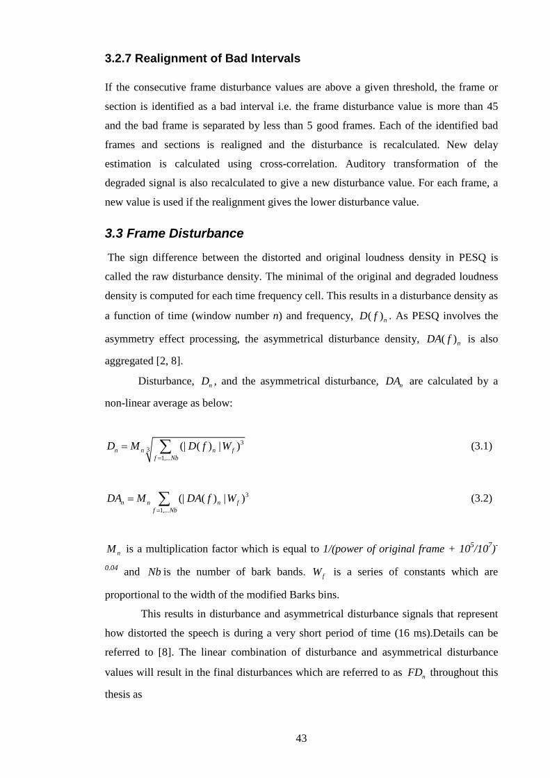
43

3.2.7 Realignment of Bad Intervals If the consecutive frame disturbance values are above a given threshold, the frame or

section is identified as a bad interval i.e. the frame disturbance value is more than 45

and the bad frame is separated by less than 5 good frames. Each of the identified bad

frames and sections is realigned and the disturbance is recalculated. New delay

estimation is calculated using cross-correlation. Auditory transformation of the

degraded signal is also recalculated to give a new disturbance value. For each frame, a

new value is used if the realignment gives the lower disturbance value.

3.3 Frame Disturbance

The sign difference between the distorted and original loudness density in PESQ is

called the raw disturbance density. The minimal of the original and degraded loudness

density is computed for each time frequency cell. This results in a disturbance density as

a function of time (window number n) and frequency, ( )nD f . As PESQ involves the

asymmetry effect processing, the asymmetrical disturbance density, ( )nDA f is also

aggregated [2, 8].

Disturbance, nD , and the asymmetrical disturbance, nDA are calculated by a

non-linear average as below:

33

1,...(| ( ) | )n n n f

f NbD M D f W

=

= ∑ (3.1)

3

1,...(| ( ) | )n n n f

f NbDA M DA f W

=

= ∑ (3.2)

nM is a multiplication factor which is equal to 1/(power of original frame + 105/107)-

0.04 and Nb is the number of bark bands. fW is a series of constants which are

proportional to the width of the modified Barks bins.

This results in disturbance and asymmetrical disturbance signals that represent

how distorted the speech is during a very short period of time (16 ms).Details can be

referred to [8]. The linear combination of disturbance and asymmetrical disturbance

values will result in the final disturbances which are referred to as nFD throughout this

thesis as

44

n n nFD D DA= + (3.3)

Figure 3.6 illustrates the concept of applying log( )nFD for controlling the

perceptual quality of the degraded signal or received signal, ny used in this research.

The original signal and the degraded signal are required for the PESQ at the transmitter

to calculate the frame disturbances for each frame.

These calculated frame disturbances can then be used for controlling functions

of the transmitter such as the transmission power, channel coding, or speech codec rate

to maintain a required quality level. In the absence of ny at the transmitting side the

PESQ must use an approximation of ny .

One possibility for calculation of log( )nFD at the transmitting side, where the

control is applied, is to use the FEP information through FQI which has been

successfully applied before [2, 4, 81, 82].

As PESQ required both degraded and reference signals at the transmitter to

evaluate the perceptual speech quality and hence calculate the nFD and subsequently,

log( )nFD , a synthesized degraded speech signal has been used. Approximation of the

degraded signal is obtained by applying an FQI feedback method which is associated

with the FEP. The MOS correlation between the usages of synthesized signal replacing

the actual degraded signal is impressively high i.e. between 0.82 and 0.91.

Figure 3.6: log( )nFD concept in controlling perceptual quality.

Transmitter Channel Receiver

PESQ

Degraded frames,

ny

nx ny log( )nFD


CUSUM/EWMA

nFQI

Original frames,

ny

45

3.4 FQI Feedback Method Output at the speech encoder gives various bits of data which have unequal perceptual

importance. Hence, the bits are often rearranged according to their perceptual

importance before applying error protection against the transmission errors. Then,

consequently, those bits which are more important for the reconstruction of speech will

be protected more effectively compared with those which are less important.

The Third Generation (3G) UMTS Adaptive Multi-Rate (AMR) is adopted in

this research. In a 3G AMR the encoded speech bits within a 20ms speech frame are

rearranged based on their perceptual importance. They are classified into the most

important bits; class A, class B and the least important, class C bits [83]. The errors in

class A can cause severe damage to speech reproduction, whereas class B and class C

bit errors can be tolerated. Therefore for a typical implementation, class A bits are

protected by rate-1/3 Convolutional Coding (CC), class B bits with rate-1/2 CC and

class C bits may be not protected at all. As an extra in error protection, an error-

concealment mechanism is also provided to mask the effects of the class A bit errors at

the receiver [84].

Figure 3.7 shows the classification of the encoded speech bits and their unequal

error protection scheme for UMTS.

Figure 3.7: The classification of the encoded speech bits and their unequal error

protection scheme for UMTS.

Error-concealment is based on a Cyclic Redundancy Check (CRC) which is

correspondent to the FQI. In a cellular system, every transmitted frame is sent with a

CRC word. The CRC is used for checking integrity of the received frame before going

through speech decoding. If there are bit errors in class A which caused the frame

Digitized Speech

AMR speech Codec

Class A bits

Class A bits

Class A bits

CRC

Rate 1/3

Rate 1/2

Rate 1/2

Convolutional Coding

46

erasure, it is indicated by failure of CRC. That frame is called a ‘bad’ frame. That

particular class A bit is replaced with the corresponding bits from the last frame which

has free error class A bits.

For estimation of perceptual speech quality, the FEP is sent back to the transmitter

through a FQI feedback method in which the receiver sends information back to the

transmitter to indicate whether the received frame was “good” or “bad”.

The FQI is binary flagged with “good=0” and “bad=1” indicating that the received

frame should be erased or not. Figure 3.8 shows the block diagram of FQI feedback

method with the conjunction of PESQ which is used in this research.

Figure 3.8: Block diagram of FQI feedback method. In this diagram, a corresponding binary signal, denoted by nFQI , is sent back to

the transmitter where n is the frame number. At the transmitter, the copies of the

transmitted frames are tagged with the corresponding nFQI for the received frames.

These frames are then sent to the speech decoder. The output of the decoder is a

synthesised version of the degraded signal, ny . Subsequently, the frame disturbance of

frame of the synthesized signal is calculated by the PESQ algorithm.

Differing from its commonly used counterparts; the FQI feedback method

utilizes the acoustic information present in the received signal at the receiver. So, its

estimation of the perceived quality is a true measure and not just based on its statistical

expectations.

Speech Encoder

PESQ Speech Decoder

Physical Layer

Speech Decoder CRC Check

Delay

Original

signal, nx

Degraded signal, y(n)

Frame disturbance,

nFD Synthesized degraded signal, ny

Rx Frame + CRC

Rx Frame + FQI

nFQI

+ FQI=0 if CRC is “good” FQI=1 if CRC is “bad”


Tx Frame

Tx Frame + FQI

Delay

47

3.5 CUSUM A cumulative sum control chart was initiated by Page in 1954 [7] and has been studied

by many researchers such as Ewan (1963) [85], Lucas (1976) [86], Gan (1991) [87] ,

Hawkins (1981,1993) [88], and Woodall and Adams (1993) [89]. Among many

schemes of control charts, it was argued that CUSUM charts are the most appropriate

and very relevant to quality control [85, 90, 91]. The CUSUM technique is also among

the most powerful tools for detecting a shift from a wide range of distribution. It is

naturally applied to the normal distributed data [92].The extension of this technique has

been explored by many researchers. It started with the application of the CUSUM chart

in economic projects to control the process average with a normally distributed quality

characteristic [93]. This technique is employed in determining the optimum values of

the sample size, the sampling interval and the decision limit.

In current practice, formulae and equations presented by Montgomery were used

[68]. The application of CUSUM charts for monitoring process average and variability

has been introduced. A CUSUM chart is directly incorporated with the whole

information in the sequence of sample values by plotting the cumulative sums of the

sample values deviations from the target value. Let the sample size1 be s > 1, jx is the

average of the jth sample and 0µ is the target value for the process average, the

CUSUM control chart up to the frame N is formulated as below

01( ),

N

n jj

C x µ=

= −∑ (3.4)

where nC is the cumulative sum including the Nth frame, since the CUSUM control chart

combines information from several samples. Due to the combination, CUSUM charts

are more effective than the common control chart, (Shewhart chart) for detecting a small

process shift. Furthermore, CUSUM is particularly effective with sample size, s = 1

[68]. If the process maintains control at the target value 0µ , the CUSUM defined in (3.4)

describes a random method with a zero average. However, if the average changes

upwards to some value 1 0µ µ> , then an ascendant tendency will develop at the CUSUM

nC . Reciprocally, if the average changes downward to some value 1 0µ µ< , the CUSUM

1 Sample size in this case is the sample size per calculation which is the number of

measurements used to calculate each value in the CUSUM.

48

will have a negative direction. If there is a tendency up and down at the limit lines, it

must be considered as evidence that the process average was changed, and the cause of

that change must be investigated and rectified.

There are two ways of representing the CUSUM charts: the algorithmic or

tabular CUSUM [68, 94] and the V-mask form of the CUSUM [86, 95, 96].

3.5.1 Tabular CUSUM

Tabular CUSUM will be used in this research. Tabular CUSUM works by accumulating

derivations from 0µ those are above target and below target with statistics C+ and

C− accordingly. Statistics C+ and C− are called one-sided upper and lower CUSUM,

respectively. With the log of frame disturbance variable nFD which has a normal

distribution (refer to Section 4.1) with mean, µ , and standard deviation,σ ,

log( ) ~ ( , )nFD N µ σ , the cumulative sums for detecting upward and downward shifts in

the mean are calculated as below

1 0max[0, log( ) ( )]n n nC C FD Kµ+ +−= + − + for an upward shift (3.5)

1 0min[0, log( ) ( )]n n nC C FD Kµ− −−= + − − for a downward shift (3.6)

where 0µ is the target mean and K is usually called the reference value or the

allowance, or the slack value. K is often chosen about halfway between the target mean

and the out of control value of the mean 1µ that we are interested in detecting quickly.

The starting value for C+ = C− = 0.

The tabular CUSUM is designed by choosing values for the reference value K

and the decision interval or threshold H . There are two thresholds H in tabular CUSUM

called upper CUSUM and lower CUSUM limits. Usually; these parameters are selected

to provide good Average Run Length (ARL) performance. ARL is the average number

of points which must be plotted before there is a point which indicates out of control

limits. Define, 0H hσ= and 0K kσ= , where 0σ is the standard deviation of the sample

variable used in performing CUSUM whereas in this research, the case is the log( )nFD .

Using 4h = or 5h = with 1/ 2k = will generally provide a CUSUM that has good

ARL properties for the shift of 1σ .

49

Note that C+ and C− accumulative deviations from the target value 0µ that are

greater than K , with both quantities reset to zero upon becoming negative. If either C+

or C− exceeds the decision interval/threshold, H , the process is considered to be out of

control.

The reasonable value for H is five times the process standard deviationσ .

Upper CUSUM is the threshold at the positive side (+H), whereas lower CUSUM is the

threshold for the negative side (-H).

Figure 3.9 shows the sample of tabular CUSUM based on Table 3.2 which shows the

sample values of log( )nFD and the value of upward and downward CUSUM. Process

standard deviation, 0σ = 0.120, k =1/2 and h = 4.. Therefore, K = 0.060 and H = 0.478.

Subsequently, the upper and lower CUSUM are 0.478 and -0.478 respectively. The

target value 0µ is set to be 0.781. The value of initial CUSUM, 0C + = 0C − = 0.

Table 3.2: The parameters for the sample of Tabular CUSUM chart.

To illustrate the calculation, consider period 1. The equation for C+ and C− are

as follows:

1 0 0max[0, log( ) ( )]nC C FD Kµ+ += + − +

Period n log( )nFD C+ C- 1 0.696 0.000 -0.025 2 0.847 0.006 0.000 3 0.785 0.000 0.000 4 0.841 0.000 0.000 5 0.765 0.000 0.000 6 0.840 0.000 0.000 7 0.941 0.100 0.000 8 0.550 0.000 -0.172 9 0.639 0.000 -0.254 10 0.882 0.041 -0.093 11 0.768 0.000 -0.047 12 0.791 0.000 0.000 13 0.918 0.077 0.000 14 0.892 0.128 0.000 15 0.847 0.134 0.000 16 0.868 0.161 0.000 17 0.898 0.217 0.000 18 0.569 0.000 -0.153 19 0.687 0.000 -0.187 20 0.600 0.00 -0.308

50

1 max[0,0 0.696 (0.781 0.060)]C + = + − +

max[0, 0.145]0

= −=

1 0 0min[0, log( ) ( )]nC C FD Kµ− −= + − −

min[0,0.696 (0.781 0.060)]min[0, 0.025]

0.025

= − −= −= −

Sample of Tabular CUSUM

-0.6000

-0.4000

-0.2000

0.0000

0.2000

0.4000

0.6000

1 2 3 4 5 6 7 8 9 10 11 12 13 14 15 16 17 18 19 20

Sample

Cus

um C

hart Upper Cusum

C+

C-

Lower Cusum

Figure 3.9: Sample of Tabular CUSUM.

The CUSUM variables C+ and C− are compared against appropriate thresholds

for detection of upward or downward shifts. The thresholds are chosen based on the

trade off between the responsiveness of the algorithm and the probability of a false

detection. Generally, thresholds that lead to faster detection of a shift in the mean will

also result in higher probability of false alarms or false detection [97].

Whenever a process shift is detected as out of control, the search for the

assignable cause will be carried out, and corrective action is required then, the CUSUM

chart will be reinitialized to zero. The CUSUM is particularly helpful in determining

when the assignable cause has occurred.

+H

-H

51

3.5.2 The V-mask

The V-mask control scheme is the alternative to Tabular CUSUM and was proposed by

Barnard in 1959 [95]. It is applied to the successive values of the CUSUM statistic as

below:

11

n

n j n nj

C y y C −=

= = +∑ (3.7)

where 0( ) /n ny x µ σ= − . Figure 3.10 shows the typical V-mask.

Figure 3.10: A sample of out of control V-Mask [98].

In this control scheme, the V-mask is formed by plotting V-shaped limits. The

V-mask is placed in the CUSUM control chart with an Origin point on the last value of

nC and the Origin-Vertex line is parallel to the horizontal axis. The process is in control

if all the previous CUSUM values ( 1 2, ,... nC C C ) lie between the upper arm and lower

arm. On the other hand, the process is considered out of control if any of the previous

CUSUM values lie outside both arms. However, in actual use, the V-mask would be

applied to each new point of the CUSUM chart as soon as it was plotted.

nC

n

52

The performance of the V-Mask is determined by the d distance and θ value as

shown in Figure 3.10.

Johnson [99] recommended the optimum values of d and θ using the following

equations:

1tan ( )2Aδθ −= (3.8)

and

2

2 1( ) ln( )d βδ α

−= (3.9)

where α , β and δ are the variables that have to be chosen appropriately. α is the

probability of a false alarm where 2α is the highest allowable probability of a signal

when the process mean is under control and β is the probability of not detecting a shift

of size δ . The A value is a scale factor chosen to make the resulting graph easily

readable as shown in Figure 3.11. Many computer programs used Johnson’s method, i.e.

Statgraphics which used the default value for each parameter as follows:

1, 0.05,δ α= = and 0.05β = [68].

Figure 3.11: The physical distance between subgroup samples is equivalent to a

unit on the vertical axis.

The application of V-mask was established and modified by Lucas in [86, 96].

Due to its complexity, the V-mask method is not always practical when applied such as

in this research application. There is a difficulty in determining how far backwards the

arms of the V-mask should extend in the case of applying V-mask for each new point of

A

1

a

2 3 a

53

CUSUM value. Furthermore, an ambiguous association with α and β may cause a

severe problem of V-mask application. Hence, the tabular CUSUM control scheme is

adopted in this research.

3.6 EWMA

An alternative technique to detect small shifts is to apply the EWMA which was

developed by S.W. Roberts in 1959 [100]. EWMA was found to be more efficient for

monitoring stationary auto correlated processes [101] and the mean of skewed

populations [102].

The EWMA control chart is also good in detecting a small shift like CUSUM.

It’s approximately equivalent to CUSUM and is easy to set up and operate. Like

CUSUM, it’s typically used with individual observations. The EWMA is often superior

to the CUSUM charting technique for detecting “larger” shifts and, unlike CUSUM, is

not sensitive to normality assumption [103]. It is sometimes called a Geometric Moving

Average (GMA) and is used extensively in time series modelling and in forecasting

[104, 105]. EWMA is defined as [106]

1log( ) (1 )n n nz FD zλ λ −= + − (3.10)

where n is the number of frame to be monitored and 0 1λ< ≤ is a constant and the

starting value is the process target, so that

0 0z µ=

Or the starting value of preliminary data i.e. the mean of several log( )nFD data, can be

used as the starting value of EWMA, so that

0 log( )nz FD=

As log( )nFD values are independent random variables with the variance 2σ ,

then the variance of nz is

2 2 2( [1 (1 ) ])2n

nz

λσ σ λλ

= − −−

(3.11)

54

Therefore, similar with CUSUM, a EWMA control chart would be constructed by

plotting EWMA values, nz versus the frame number n or time. This is different from

CUSUM which have a constant control limits. The centre line, upper and lower control

limits for EMWA control charts are dependent on the target value 0µ and the number of

frame n as follows:

20 [1 (1 ) ]

(2 )nUCL L λµ σ λ

λ= + − −

− (3.12)

0CL µ= (3.13)

20 [1 (1 ) ]

(2 )nLCL L λµ σ λ

λ= − − −

− (3.14)

where σ and n is the standard deviation and frame number of the data. The factor L is

the width of the control limits.

In general, values of λ in their interval 0.05 0.25λ≤ ≤ work well in practice,

with 0.05λ = , 0.10λ = and 0.20λ = being popular choices. A good rule of thumb is to

use the smaller values of λ to detect smaller shift. By research (Hunter, 1989) [107],

the value of λ = 0.4 and 3.054L = is recommended.

As n gets larger, the control limits will approach steady-state values given by the

following equations:

0 (2 )UCL L λµ σ

λ= +

− (3.15)

0 (2 )LCL L λµ σ

λ= −

− (3.16)

Figure 3.12 shows a sample of a EWMA chart based on sample values shown in

Table 3.3. Similar to CUSUM, the EMWA values, nz is under control if it is not beyond

the upper and lower limit of the EWMA chart. Table 3.3 shows the sample values of

55

log( )nFD , nz and the value of upper and lower control limit of EWMA. The target

value, 0µ = 0.356, L = 3, σ = 0.079 and 0.2λ = were selected appropriately.

Table 3.3: EWMA parameters for the sample of EWMA chart.

log( )nFD nz UCL LCL 0.268 0.338 0.404 0.308 0.368 0.344 0.417 0.295 0.353 0.346 0.424 0.288 0.321 0.341 0.428 0.283 0.429 0.359 0.431 0.281 0.356 0.358 0.433 0.279 0.401 0.367 0.434 0.278 0.428 0.379 0.434 0.278 0.311 0.365 0.435 0.277 0.201 0.332 0.435 0.277 0.323 0.331 0.435 0.277 0.383 0.341 0.435 0.277 0.368 0.346 0.435 0.277 0.293 0.336 0.435 0.277 0.211 0.311 0.435 0.277 0.460 0.341 0.435 0.277 0.292 0.331 0.435 0.277 0.412 0.347 0.435 0.276 0.377 0.353 0.435 0.276 0.528 0.388 0.435 0.276

0.2445

0.2945

0.3445

0.3945

0.4445

0.4945

1 2 3 4 5 6 7 8 9 10 11 12 13 14 15 16 17 18 19 20

EWM

A

Sample

EWMA Chart

Average

UCL

LC

Figure 3.12: Sample of EWMA chart.

56

To illustrate the calculations, consider the first observation 1log( ) 0.268FD = .

The first value of EWMA 1z is

1 1 0(log ) (1 )z FD zλ λ= + −

(0.2)(0.268) (1 0.2)(0.356)0.338

= + −=

Therefore, 1z = 0.338 is the first value plotted in Figure 3.12. The second value of

EWMA 2z is

2 2 1log( ) (1 )z FD zλ λ= + −

(0.2)(0.368) (1 0.2)(0.338)0.344

= + −=

The other values of the EWMA are computed similarly.

The control limits in figure 3.12 are found using equation (3.12) and (3.14). For

n = 1,

20 [1 (1 ) ]


λ= + − −

−

2(1)0.20.356 (3)(0.079) [1 (1 0.2) ]

(2 0.2)0.404

= + − −−

=

and

20 [1 (1 ) ]


λ= − − −

−

2(1)0.20.356 (3)(0.079) [1 (1 0.2) ]

(2 0.2)0.308

= − − −−

=

For n =2, the limits are

20 [1 (1 ) ]


λ= + − −

−

2(2)0.20.356 (3)(0.079) [1 (1 0.2) ]

(2 0.2)0.417

= + − −−

=

and

20 [1 (1 ) ]


λ= − − −

−

57

2(2)0.20.356 (3)(0.079) [1 (1 0.2) ]

(2 0.2)0.295

= − − −−

=

As n increase the control limits increase in width until they stabilize at the steady state

values given by equations (3.15) and (3.16).

0 (2 )UCL L λµ σ

λ= +

−

0.20.356 (3)(0.079)

(2 0.2)0.435

= +−

=

0 (2 )LCL L λµ σ

λ= −

−

0.20.356 (3)(0.079)

(2 0.2)0.276

= −−

=

Similar to CUSUM applications, whenever process shift is detected to be out of

control, the search for the assignable cause will be investigated, and corrective action is

required then, the EWMA chart limit will be reinitialized to zero and the limits will be

refreshed.

Like CUSUM, the EWMA performs well against small shifts but does not react

well to large shifts as quickly as the Shewhart chart. However, EWMA is superior to the

CUSUM only for larger shifts particularly if λ > 0.1. Differing from CUSUM which is

sensitive to normality assumption, EWMA is insensitive to statistical distribution

properties and was properly designed to be less sensitive to the normality assumption

[103]. It is due to its scheme which can be viewed as a weighted average of all past and

current observations. Even, if the log( )nFD has a normal distribution, the application of

EWMA as the control tool for this research is significant in making the comparison with

CUSUM.

3.7 Closed Loop Power Control in FDD Mode

In CLPC, FDD mode is used for both uplink and downlink but TDD mode is

only used in downlink [47, 53]. Furthermore, CLPC in FDD mode is more widely used

in UMTS [66]. The CLPS procedure in UMTS is divided into two processes which are

58

outer loop and inner loop [52]. The inner loop process was discussed earlier in Chapter

2 (Section 2.3.2). The block diagram of UMTS CLPC is shown in Figure 2.10.

Outer loop operates within the BS The outer loop dynamically sets the SIR

target for the inner loop based on the FER target which is usually 1% for speech

services for achieving a satisfactory speech quality. The outer loop sets the target SIR at

the BS according to the needs of the end users and aims at a constant quality. On the

other hand, the inner loop regulates transmit power of the UE such as a hand phone in

an attempt to compensate signal amplitude fading and meet the SIR target. When the

inner loop is unable to combat channel fading, the FER will increase. Consequently the

outer loop increases the SIR target to maintain the FER target.

3.7.1 Conventional UMTS Outer Loop Power Control Algorithm

Figure 3.13 shows a commonly accepted flow chart of a conventional UMTS outer loop

power control [51]. For each received speech frame at the BS, CRC is used to check the

integrity of the frame whether it contains errors or not. If CRC detects an error in the

frame, then the SIR target is increased by K multiplies by a given step size ∆ in dB,

where K is a positive integer. The value of K is related to the desired FER as

1 1KFER

= −

(3.17)

The algorithm aims to keep the real FER less than or equal to the equation 3.18.

In its steady state, the SIR target is not far from the minimum value of SIR required to

maintain the FER target. Therefore, setting the small ∆ to decrease the excess SIR may

result in inaccurate monitoring of the channel variation and longer convergence time.

On the contrary, setting the large ∆ to increase the SIR target may result in fast channel

changes. Consequently it will lead to a larger interference and a decrease in the system

capacity [51]. Hence, the outer loop step up size up∆ and step down size down∆ can be

formulated as

up K∆ = × ∆ and down∆ = ∆ (3.18)

Note that the dynamic range of SIR target is limited. Hence, the new SIR target

is compared to the allowed minimum and maximum limits of the SIR target. If the SIR

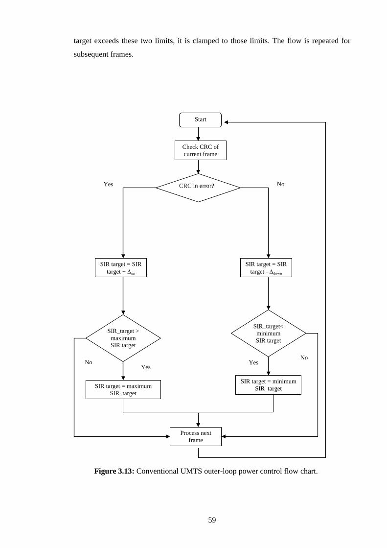
59

target exceeds these two limits, it is clamped to those limits. The flow is repeated for

subsequent frames.

Start

Check CRC of current frame

SIR target = maximum SIR_target

Process next frame

SIR_target<minimum SIR target

No

No No

Yes

Yes Yes

Figure 3.13: Conventional UMTS outer-loop power control flow chart.

CRC in error?

SIR target = SIR target + ∆up

SIR target = SIR target - ∆down

SIR_target > maximum SIR target

SIR target = minimum SIR_target

60

3.8 SPC Based UMTS Power Control

In the SPC based UMTS power control model shown in Figure 3.3, perceptual speech

quality is measured by PESQ. The FD which is subtracted from PESQ will be utilized

by the SPC and then the statistical value of FD is applied in the outer-loop power

control. This SPC based technique employs the PESQ reference implementation

software supplied by ITU [108]. A delay was introduced to account for the round-trip

delay between the AMR encoder and the decoder at the transmitter.

Minor modifications were made to the reference implementation to integrate

PESQ in the simulation model. In the simulations, level alignment in the reference

implementation of PESQ was disabled in order to speed up simulations. Furthermore,

the performance of PESQ with and without level alignment were confirmed to be

identical [4]. Some additions of interfacing code (wrappers) to the original C code of the

reference implementation of PESQ also have also been made in order to integrate PESQ

into Matlab Simulink.

Figure 3.14 shows a flow chart for the SPC based outer loop power control. The

difference between the conventional and the SPC based outer loop power control flow

chart is highlighted in the chart. Compared with the conventional power control, there is

an additional process after CRC indicates an error in Class A bits of the received frame.

The SIR target is not automatically increased but is only increased if the FD statistical

data is higher than the SPC upper limits. Otherwise, the SIR target will be decreased. In

a case where the FD statistical data is less than the SPC lower limit, the SIR target will

also be decreased. Hence, the scheme will ensure that the perceptual speech quality

received by the end user meets the customer requirement and at the same time optimizes

the power usage in the system.

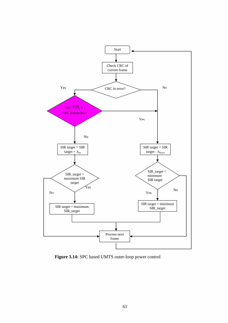
61

Start


log ( nFD ) < SPC thresholds?


Process next frame

SIR_target < minimum SIR target

No

Yes

No No

Yes

Yes

No

Yes

Figure 3.14: SPC based UMTS outer-loop power control

CRC in error?



SIR_target > maximum SIR

target


62

3.9 Summary The proposed perceptual speech quality control technique was described thoroughly in

this chapter. In this technique, the log( )nFD parameter which is subtracted from PESQ

is replaced by a non-perceptual metric such as FER in mobile communication systems.

The details of PESQ components are briefly described as well as the FD. The statistical

analysis of FD is discussed in Chapter 4.

As PESQ required both degraded and reference signals at the transmitter to

evaluate the perceptual speech quality and hence calculate the FD, the synthesized

degraded speech signal has been used. Approximation of the degraded signal is obtained

by applying the FQI feedback method which is associated with the FEP. This method

was deliberated thoroughly in this chapter.

The novelty of this thesis which is a direct control approach using SPC was

discussed. This approach is the first attempt in a mobile communication system. Two

prominent tools from SPC are considered for the purposes of this perceptual speech

quality control: CUSUM and EWMA, which were discussed in Sections 3.5 and 3.6.

CUSUM has two ways of representing the CUSUM operation chart: tabular CUSUM

and V-mask form. Due to the complexity of the V-mask form application, tabular

CUSUM was adopted to apply in the proposed application. Both, CUSUM and EWMA

are well-known as the tools which have the greatest ability in monitoring the small

changes in the process mean. As applied to the outer loop power control in a UMTS, the

performance comparison between both tools is represented in Chapter 5.

The UMTS closed loop power control in FDD mode which is applied in this

research is discussed including details of the conventional UMTS outer loop and inner

loop power control. Subsequently, the proposed SPC based Power Control which is new

in a communication system is described.

63

CHAPTER 4

THE CUSUM TECHNIQUE APPLICATION IN PERCEPTUAL SPEECH QUALTY CONTROL

4.0 Introduction

Power control is an important means of providing a fair operating environment among

all users. An adequate QoS for a speech user can be measured in terms of PESQ, and as

such accurate power control operates to minimize interference among all users and at

the same time providing an adequate QoS as required in UMTS.

Therefore, in this chapter, the speech codec rate and power control using a

CUSUM based technique is applied in UMTS to improve the performance of UMTS.

This chapter begins with an analysis of the FD which is subtracted from PESQ. Then,

the application and analysis of the CUSUM based technique for controlling the speech

codec rate and power control in Universal Mobile Telecommunication Systems

(UMTS) is discussed. This is followed by the experimental results and ends with a

summary of the chapter.

The distributions of this chapter are as follows:

• Presentation of the FD analysis. It is observed that the log( )nFD have a log-

normal distribution for a given perceptual quality MOS.

• Application of a CUSUM based speech codec rate control for UMTS is

presented. CUSUM based technique allows faster action at the transmitter to

control the quality of the speech signals as required by the end users. Hence,

the conventional parameter such as FER can be replaced with the log( )nFD .

• Comparison of the performance of CUSUM based and FER based outer loop

power control algorithm through simulations. It is shown that the CUSUM

based power control achieves adequate speech quality while reducing the

average SIR target by up to 13% relative to the conventional algorithm.

64

4.1 Frame Disturbance Analysis

Details of the FD are described in Section 3.3. In this section, the simulation and the

analysis of FD distribution is presented.

4.1.2 Input speech file and speech codec Input speech samples used in the analysis are from the ITU database for speech quality

measurement tests. Each speech file contained pre-recorded sentences of 8s duration

with approximately 50% speech and 50% silence intervals. However, FD is calculated

with the silence periods removed to ensure only the active speech is considered in this

application. The AMR speech codec is a standard codec for UMTS and was used in the

analysis at the transmitter and receiver part

4.1.3 Methodology In the absence of a degraded speech signal at the transmitter site, an approximation must

be used. In this case, the FQI method is applied to synthesize the speech signal output as

shown in Figure 4.1. A degraded speech signal with PESQ MOS ranging 3.0 to 3.5 is

collected and saved. In attaining more reliable FD distribution, for each PESQ MOS, 10

sets are collected where each set contains FD which is presented by 10 speech files.

Each speech file on average contains 243 samples of FD calculations. The silence parts

of the speech signal output were removed for this analysis. The simulation model is as

shown in Figure 4.1. The estimated mean and standard deviation of the distribution of

each PESQ MOS from 3.0 to 3.5 are observed and recorded.

By applying the sample mean estimation theorem [68], the estimated mean

( )log FDn , sµ of one set of 10 speech files is given by

1[ ( )] ( )1

NE log FD log FDn n sN n

µ= =∑=

, (4.1)

where N = 2430 for 10 speech files. Consequently, the estimated mean for all 10 sets of

speech files is given by

1[ ] 01

ME s snN m

µ µ µ= =∑=

, (4.2)

65

where M = 10, and0

µ is the target mean of the ( )log FD ,n which will be used for

CUSUM based speech codec control at the next section.

Figure 4.1: Simulation model for frame disturbance analysis.

4.1.4 Simulation result and discussion The result of FD analysis is shown in Figure 4.2 over a range of PESQ MOS values.

-3 -2 -1 0 1 2 3 40

0.05

0.1

0.15

0.2

0.25

0.3

0.35

0.4

0.45

0.5

log(FDn)

Relat

ive F

requ

ency

(a)

AMR Encoder

Channel Model

AMR Decoder

PESQ ny

nFD

Synthesis Signal

nFQI

nx

Reference Signal

66

-3 -2 -1 0 1 2 3 40

0.05

0.1

0.15

0.2

0.25

0.3

0.35

0.4

0.45

0.5

log(FDn)

Relat

ive F

requ

ency

(b)

-3 -2 -1 0 1 2 3 40

0.1

0.2

0.3

0.4

0.5

0.6

0.7

Log(FDn)

Relat

ive F

requ

ency

(c)

67

-3 -2 -1 0 1 2 3 40

0.1

0.2

0.3

0.4

0.5

0.6

0.7

log(FDn)

Relat

ive F

requ

ency

(d)

-3 -2 -1 0 1 2 3 40

0.1

0.2

0.3

0.4

0.5

0.6

0.7

log(FDn)

Relat

ive F

requ

ency

(e)

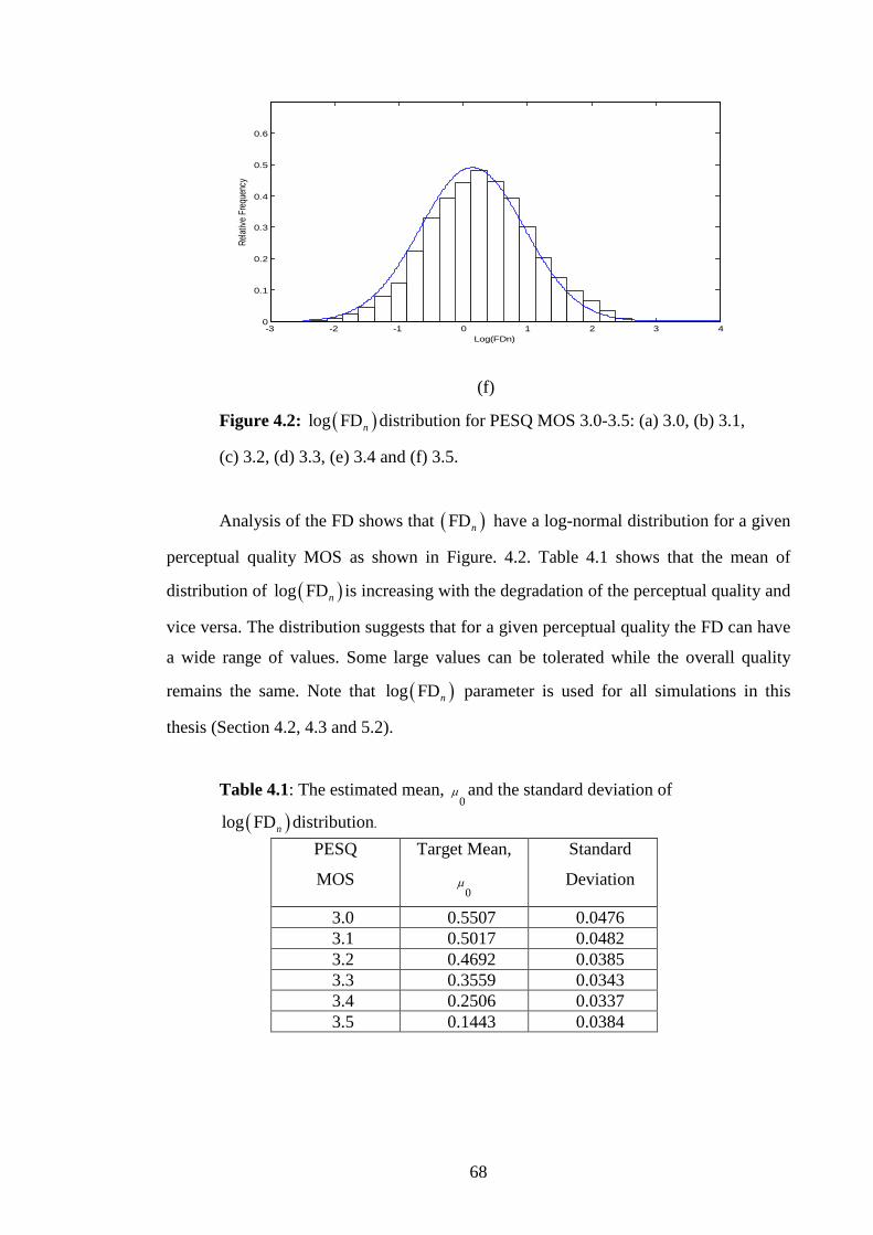
68

-3 -2 -1 0 1 2 3 40

0.1

0.2

0.3

0.4

0.5

0.6

Log(FDn)

Relat

ive F

reque

ncy

(f)

Figure 4.2: ( )log FDn distribution for PESQ MOS 3.0-3.5: (a) 3.0, (b) 3.1,

(c) 3.2, (d) 3.3, (e) 3.4 and (f) 3.5.

Analysis of the FD shows that ( )FDn have a log-normal distribution for a given

perceptual quality MOS as shown in Figure. 4.2. Table 4.1 shows that the mean of

distribution of ( )log FDn is increasing with the degradation of the perceptual quality and

vice versa. The distribution suggests that for a given perceptual quality the FD can have

a wide range of values. Some large values can be tolerated while the overall quality

remains the same. Note that ( )log FDn parameter is used for all simulations in this

thesis (Section 4.2, 4.3 and 5.2).

Table 4.1: The estimated mean, 0

µ and the standard deviation of

( )log FDn distribution. PESQ

MOS

Target Mean,

0µ

Standard

Deviation

3.0 0.5507 0.0476 3.1 0.5017 0.0482 3.2 0.4692 0.0385 3.3 0.3559 0.0343 3.4 0.2506 0.0337 3.5 0.1443 0.0384

69

4.2 Speech Codec Rate Control Simulation model

4.2.1 Introduction

A simulation model for speech codec rate control is shown in Figure 4.3 below. The

same input speech and speech codec employed for frame disturbance analysis (Section

4.1) has been used for the simulations.

Figure 4.3: The simulation model for speech codec rate control.

4.2.2 Methodology

By applying the sample mean estimation theorem [68], the estimated mean

( )log FDn of one set of 10 speech file is given by

1[ ( )] ( )1

NE log FD log FDn nN n

µ= =∑=

, (4.3)

Where N = 2430, and µ is the mean of ( )log FDn that will be used for CUSUM

application.

The speech quality perceived differs among the end users as it depends on their

judgment of perception. This CUSUM application is applied on an end user to end user

basis. Two cases will be applied using the CUSUM control chart in this analysis. The

quality of the speech was controlled to a PESQ MOS of 3.3 which is considered a good

speech quality MOS score. Hence, based on Table 4.1, the CUSUM target mean, 0

µ , is

set to be 0.3559.

AMR Encoder

Channel Model

AMR Decoder

PESQ ny log( )nFD


CUSUM

nFQI

nx

Reference Signal

70

A total of 50 sequenced speech files are simulated with the AMR initial speech

codec rate being set to 2. The mean, µ, of ( )log FDn for each speech file, was applied to

the CUSUM control chart.

Table 4.2: Parameters chosen for CUSUM chart.

K ½ σ

Upper limit 0.3512

Lower limit -0.3512

Target mean 0.3559

Initial AMR speech codec rate 2

Case 1

The first 40 speech files are 3.3 PESQ MOS while the other 10 speech files are

degraded speech files.

Case 2

The first 40 speech files are 3.3 PESQ MOS while the other 10 are the better grade of

speech files.

Process standard deviation, σ for the in controlled first 40 simulated speech files is

0.0878. K was set to be 1

2σ and H was set to be 5σ. Therefore CUSUM upper and lower

limit, H was set to be 0.3512 and -0.3512, respectively. The process mean for the first

40 simulated speech files is 0.3575. The chosen CUSUM parameters are shown in Table

4.2

71

4.2.3 Simulation results and discussion Case 1

Uncontrolled CUSUM

-0.6

-0.4

-0.2

0.0

0.2

0.4

0.6

0.8

1.0

1 3 5 7 9 11 13 15 17 19 21 23 25 27 29 31 33 35 37 39 41 43 45 47 49Speech Sample

Cus

um C

hart

Upper CusumC+C-Lower Cusum

Figure 4.4: A CUSUM control chart without controlling speech codec rate.

Figure 4.4 shows a CUSUM control chart without controlling speech quality.

The mean of process for the last 10 simulated speech files was increased to 0.4674. The

out of control CUSUM was detected at the 43rd speech signal sample at the CUSUM

upper limit which indicated there was a degradation of the speech signals.

Controlled CUSUM

-0.6

-0.4

-0.2

0.0

0.2

0.4

0.6

0.8

1.0

1 3 5 7 9 11 13 15 17 19 21 23 25 27 29 31 33 35 37 39 41 43 45 47 49Speech Sample

Cus

um C

hart Upper Cusum

C+C-Lower Cusum

Figure 4.5: Apply CUSUM with controlling speech codec rate.

72

Figure 4.5 shows that the degradation of the speech signals was rectified by

increasing the speech codec rate from mode 2 to mode 3 starting at the 44th speech

signal sample.

Case 2

Uncontrolled CUSUM

-1.0

-0.8

-0.6

-0.4

-0.2

0.0

0.2

0.4

0.6

1 3 5 7 9 11 13 15 17 19 21 23 25 27 29 31 33 35 37 39 41 43 45 47 49

Speech Sample

Cus

um C

hart Upper Cusum

C+C-Lower Cusum

Figure 4.6: A CUSUM control chart without controlling speech codec rate.

Figure 4.6 shows the CUSUM control chart without controlling speech quality.

The mean of process for the last 10 simulated speech files was decreased to 0.2446. The

out of control CUSUM was detected at 44th speech signal sample but this time it

occurred at the CUSUM lower limit. This indicated that the signal was beyond the

quality which is needed by the end user or customer.

73

Controlled CUSUM

-1.0

-0.8

-0.6

-0.4

-0.2

0.0

0.2

0.4

0.6

1 3 5 7 9 11 13 15 17 19 21 23 25 27 29 31 33 35 37 39 41 43 45 47 49

Speech Sample

Cu

sum

Ch

art

Upper CusumC+C-Lower Cusum

Figure 4.7: Apply CUSUM with controlling speech codec rate.

Figure 4.7 shows the excess quality of the speech signals was rectified by

decreasing the speech codec rate from mode 2 to mode 1 starting at 45th speech signal

sample.

4.3 Power Control Simulation Model

In this section, a CUSUM based technique as described in Chapter 3 is incorporated in

the outer-loop of the UMTS power control. The performance of this CUSUM based

technique is compared against a conventional UMTS counterpart using computer

simulations.

A Matlab Simulink implementation of the UMTS physical layer was used for

simulations. A physical layer was implemented at chip level according to the 3GPP

technical specifications2. Figure 4.8 shows a block diagram of the simulation model

showing the relevant functional blocks. The building blocks and some of the important

simulation parameters are described briefly in the following sub-sections.

2We would like to thank and acknowledge PHYBIT Inc. Singapore for permitting us to use their

UMTS physical layer simulation software.

74

Figure 4.8: Block diagram of the simulation model of UMTS physical

layer (FDD mode).

4.3.1 Input speech file For consistency, only one input speech file was used for all simulations in this chapter.

This speech file was constructed by the combination of five speech files (O_M01L1A,

O_M01L1C, O_F01L6A, O_F01L6B, and O_F01L6C) from the ITU database for voice

quality measurement tests [77]. Each of the constituent speech files consisted of 8

seconds of pre-recorded sentences with approximately 50% speech and 50% silence

intervals. Constituent speech files were recorded in 16-bit, 8 kHz linear PCM format.

4.3.2 Speech codec

The AMR speech codec has been employed for all the simulations in this chapter. This

codec which is mandatory for UMTS [78] was described in Section 3.1.3.

75

Generally, the AMR codec mode 7 produced the superior speech quality.

Therefore, this mode has been used for the simulation of this chapter. The frame

structure of AMR codec mode 7 is summarized in Table 4.3.

Table 4.3: Summary of AMR codec mode 7 frame structure.

Codec Rate

(kbps)

Number of bits

per frame

Number of

Class A bits

Number of

Class B bits

Number of

Class C bits

12.2 244 81 103 60

4.3.3 Multiplexing and channel coding In the simulation model as shown in Figure 4.8, the 20 ms encoded speech frames are

processed by “Multiplexing and Channel Encoding” which are referred to hereafter as

MC blocks. In UMTS, data arriving from Layer 2 is processed in Transmission Time

Interval (TTI). In this case, each AMR speech frame corresponds to 20 ms TTI.

Operations of the MC block in each TTI are summarized below.

Transport Channel (TrCH) allocation

In UMTS, the transmitted data can be divided into distinct logical channels which are

referred to as Transport Channels (TrCH). This separate TrCH then assigned to the

AMR output bit Class A, B, and C denoted as TrCH1, TrCH2, and TrCH3 respectively.

CRC attachment

In every TTI, a 12 bit CRC is attached to the TrCH1. The receiver uses the CRC bits to

detect any potential Class A errors. There are no CRC bits for TrCH2 and TrCh3.

Channel Coding

Convolutional coding (CH) has been recommended for speech [109]. A rate 1/3 code is

used for TrCH1 while a rate ½ code is used for both TrCH1 and TrCH2 [110].

First interleaving

Two stages of interleaving were required in UMTS to achieve the best performance.

Two stages are needed to spread the channel errors as widely as possible. The first

interleaver is an inter-frame interleaver operated individually on each TrCH for every

76

TTI. In the case of speech, TrCH bits are entered into the interleaver row-by-row, with

two columns for each row. Subsequently, the bits are set out in columns [53].

Radio frame segmentation

Data are transmitted in 10 ms radio frames in UMTS, equivalent to two radio frames per

TTI per speech. This radio frame segmentation process involves dividing data from

each TrCH into two consecutive radio frames.

Multiplexing

Transport channels are multiplexed into a simple serial multiplexing on a frame by

frame basis named Single Coded Composite Transport Channel (CCTrCH), and for this

multiplexing, each transport channel provides data in 10 ms frames.

Second interleaving

The second interleaver is an intra-frame interleaver and it operates on 10 ms radio

frames. For that scenario, the bits from a radio frame are read into the interleaver row by

row where each row contains 30 columns. Subsequently, the bits are set out in columns

after inter-column modification has been applied.

4.3.4 Power Control

In this section, simulation details of the conventional UMTS and CUSUM based power

control algorithms are given. Since the natural application of CUSUM technique

corresponds to the normal distribution [92], the application of the CUSUM in

controlling power is justified.

Conventional UMTS power control

Closed loop power control as described in Section 3.7 was simulated for the

conventional UMTS power control which incorporated both inner and outer loops. The

TPC commands for the inner loop were applied based on Algorithm 1 given in Section

2.3.2. Transmission power was updated using a step size δ of 1 dB, which is the

mandatory step size specified in [67]. An updated rate of 1500 1s− corresponds to once

every time slot. The outer loop was based on the algorithm proposed by Sampath et al.

[51]. A flow chart of the algorithm is shown in Figure 3.14. The FER target for the

algorithm was set to 1%., and the SIR target was updated using a step size ∆ of 0.005

dB [47] at a rate of 50 1s− which corresponds to once every speech frame. A summary

77

of the simulation parameters for the conventional UMTS power control is given in

Table 4.4. Table 4.4: Conventional UMTS power control parameters.

Type Algorithm Update

rate( 1s− )

Step up

size(dB)

Step down

size(dB)

FER

Target(1%)

Outer Loop Sampath et al 50 ∆up = 0.495 ∆down =

0.005

1

Inner Loop Algorithm 1 1500 δ up = 1 δ down = 1 -

CUSUM based UMTS Power Control

Simulation model for UMTS power control based on CUSUM is as described and

illustrated in Chapter 3. Figure 4.9 shows the application of CUSUM based in UMTS

outer-loop power control.

Figure 4.9: Application of CUSUM in UMTS outer-loop power control.

A flow chart for the CUSUM based outer loop power control is depicted in

Figure 4.10 based on Figure 3.15 (Chapter 3, section 3.8).


Channel

CUSUM ny

Synthesized Signal

log( )nFD PESQ

AMR Decoder

CRC Check FEP

( nFQI )

AMR Decoder

Delay

+

Delay

Reference Signal

Speech Signal

Received Signal


78

Start


log ( nFD ) < CUSUM

thresholds?


Process next frame


No

Yes

No No

Yes

Yes

No

Yes

Figure 4.10: CUSUM based UMTS outer-loop power control

CRC in error?




target


79

4.3.5 Channel

In the mobile radio channel, noise sources can be subdivided into multiplicative and

additive effects. The simplest practical case of a mobile radio channel is an additive

white Gaussian Noise (AWGN) channel [111].

For the purpose of simulations, a 6-ray Vehicular A channel model specified by

3GP [112, 113] has been considered for modeling the fast multipath channel. Relative

time delays and average powers for each path of the channel models are summarized in

Table 4.5. Power Spectral Densities (PSD) for each path follows the classical PSD

[114]. The logarithm scale shadowing was modeled according to the correlated normal

distribution. Normally, the mean value of the distribution is practically equal to the path

loss. However, in this research, the path loss was assumed to be compensated for by the

power control subsystem which implies that the mean of the distribution is equal to 0

dB. The standard deviation of the distribution is the function of the propagation

environment. For urban environments, an 8 dB standard deviation has been used [115]

Furthermore, a de-correlation distance of 20 m has been used in this model [116]. De-

correlation distance is the signal shadowing which it de-correlates with travel distance

and it is dependent on the propagation environment.

Table 4.5: Tapped-delay-line parameters for Vehicular A environment [113].

Tap Number Relative Delays

(ns)

Relative Avg

Power (dB)

Doppler Spectrum

1 0.0 0.0 Classical

2 310 -1.0 Classical





80

4.3.6 Summary of simulation parameters

A summary of main simulation is given in Table 4.6. From this table it is noted that the

K and CUSUM target are set to be 12

σ and 0.02 respectively, where σ is the process

standard deviation. Based on FD analysis at section 4.1, the CUSUM target of 0.02 was

found to be equivalent to an MOS score of 4.0 for PESQ. The PESQ MOS starts

deteriorating rapidly once it reaches the value 3.6 for the AMR codec mode 7 (12.2 kbs)

[80]. Therefore, the chosen CUSUM target was appropriate to ensure that the CUSUM

based power control activates SIR target reduction only when the quality is good.

4.3.7 Methodology

Based on 3GPP recommendations [112], three representative vehicular speeds f 3, 50,

and 120 km/h were employed for performance comparison between conventional and

CUSUM based UMTS power control algorithm. To ensure the channel error patterns

were independent for the simulations, 5 different channels shadowing profiles were

simulated for each vehicular speed. Each power control algorithm was simulated for

outer loop step sizes of ∆ of 0.005, 0.01, 0.015 and 0.02 dB. For each simulation, a 40 s

speech file was transmitted on the UMTS physical layer shown in Figure 4.8 enabling

only one power control algorithm at a time. In each case, the variations of the SIR target

and the channel shadowing profile were recorded.

For each simulation, the PESQ algorithm was applied to the received speech file

together with the original transmitted file and the corresponding actual PESQ MOS was

calculated.

81

Table 4.6: Main simulation parameters.

_____________________________________________________________________

Chip rate 3.84 Mc/s

Spreading factor 128

Channel bit rate 60 kb/s

Speech coding AMR (rate 12.2 kb/s)

Channel Coding

Class A Rate 1/3 CC + 12 bit CRC

Class B Rate 1/2 CC

Class C Rate 1/2 CC

Interleaving both inter and intra-frame

Modulation QSPK

Power Control

Inner Loop

Update rate 1500s-1

Up/down step size (δup or δdown) 1 dB

Outer-Loop (Conventional)

FER target 1%

Control variable CRC flags

Step down ∆down 0.005, 0.01, 0.015 and 0.02 dB

Step down ∆up 0.495, 0.99, 1.485 and 1.98 dB

Update rate 50 s-1

Outer-Loop (CUSUM based)

FER target 1%

Control variable CUSUM threshold and CRC flags

CUSUM target 0.02

Step up/down as conventional above

Update rate 50 s-1

Channel type

AWGN ON

Log-normal Fading ON

(Std, decorrelation distance) (8 dB, 20 m)

Fast Fading 6-tap Vehicular A

Vehicular speed 3, 50 and 120 km/h

Receiver Rake (6 fingers)

Initial SIR 4 dB

82

4.3.8. Simulation results and discussion

Simulation results for each outer loop step sized and vehicular speed of 3, 50, and 120

km/h are given in Table 4.7(a)-(c), Table 4.8(a)-(c), Table 4.9(a)-(c) and Table 4.10(a)-

(c) respectively. These results include the average and standard deviation of the SIR

target and the PESQ MOS corresponding to two different power control algorithms

obtained for each shadowing profile. Furthermore, the gain of the CUSUM based power

control with respect to the conventional power control calculated as the difference

between the SIR targets in the two cases is shown. Ensemble averages over all

shadowing profiles are also included.

A statistical significant difference between the two methods is obtained by

applying the T-test statistic. In this statistical significance testing, p-value is the

probability of obtaining a test statistic at least as extreme as the one which was actually

observed. If the p-value is less than the significance level α (Greek alpha), which is

often 0.05 or 0.01 [117], the result is said to be statistically significant.

Table 4.7(a)-(c), Table 4.8(a)-(c), Table 4.9 (a)-(c) and Table 4.10(a)-(c) shows

the p-value is less than the significance level, therefore, the result is consider to be

statistically significant.

From the Table 4.7(a)-(c), Table 4.8(a)-(c), Table 4.9(a)-(c) and Table 4.10(a)-

(c), it is observed that the CUSUM based power control achieved from 3% to 14% gains

in the SIR target. The perceptual quality of CUSUM based technique in term of PESQ

MOS is kept in all cases within a desired range 3 to 3.5 of “fair” to “good” quality. All

the PESQ MOS differences are less than 0.2 MOS and hardly perceptible. Therefore,

we could say that both power control algorithms deliver adequate perceptual qualities,

even though, at different cost in terms of average SIR target levels.

It is also observed that generally, perceptual quality delivered by the

conventional technique power control is slightly higher than a CUSUM based

technique. The reason for this observation was the ability of the perceptual scheme to

trade-off average transmitting power with perceptual quality in a more controlled

manner. On the other hand, inefficiencies in conventional power do not allow for

precise control of the speech quality. Network providers have to balance their desire to

increase capacity by reducing the average of SIR level, and their commitment to provide

adequate quality to customers, which is achieved by power control. However,

inefficiencies in a conventional technique will tip the balance one way or the other. That

is, at times more than necessary quality is provided, at a cost of extra power and hence

83

reduced capacity while at other times quality is degraded and is being sacrificed to gain

higher capacity. On the other hand, a CUSUM based technique always provides

adequate perceptual quality and at the same time, avoids situations where a

conventional technique provides more than necessary quality at the cost of increased

average SIR target. Therefore, we can say that a CUSUM based technique does a better

“balancing” act than its counterpart. It should also be noted that the same gains could

not be achieved by allowing a larger FER target for conventional power control without

affecting the perceptual quality more severely [80]. In this case, the FER is increased

regardless of the effect on the perceptual quality, whereas with CUSUM based power

control, the FER is only increased when the quality is not affected noticeably.

SIR target gain is due to the number of times a CUSUM based algorithm avoids

increasing the SIR target while the conventional algorithm could not manage it. That is,

a lower SIR target corresponds to more efficient power control. In this case, the gain

increased with the power control step size as noted in the Table 4.7(a)-(c), Table 4.8(a)-

(c), Table 4.9(a)-(c) and Table 4.10(a)-(c).

84

Table 4.7: Results for conventional and CUSUM based power control

algorithms with outer-loop step down, ∆down = 0.005 dB and vehicular speed of

(a) 3 km h-1, (b) 50 km h-1 and (c) 120 km h-1.

(a)

Channel Profile Ave SIR target(dB) PESQ MOS Conv Std CUSUM std Gain CUSUM P value Conv CUSUM Difference

profile 1 4.075 0.164 3.932 0.121 0.143 3.87E-35 3.169 3.057 0.112 profile 2 4.112 0.081 3.845 0.119 0.267 0.00E+00 3.205 3.177 0.028 profile 3 4.058 0.068 3.848 0.124 0.210 0.00E+00 3.152 3.034 0.118 profile 4 4.081 0.152 3.887 0.122 0.194 3.24E-19 3.048 3.016 0.032 profile 5 4.022 0.061 3.957 0.119 0.065 4.16E-155 3.153 3.100 0.053 Average 4.070 0.105 3.894 0.121 0.176 6.48E-20 3.145 3.077 0.069

(b)


profile 1 4.260 0.097 3.966 0.229 0.294 4.27E-15 3.016 2.982 0.034 profile 2 4.125 0.062 4.091 0.128 0.034 0.00E+00 3.152 3.006 0.146 profile 3 4.190 0.083 4.022 0.129 0.168 3.83E-15 3.095 2.967 0.128 profile 4 4.134 0.073 3.998 0.125 0.136 1.20E-25 3.201 3.171 0.030 profile 5 4.124 0.095 3.849 0.090 0.275 0.00E+00 3.083 2.997 0.086 Average 4.167 0.082 3.985 0.140 0.181 1.62E-15 3.109 3.024 0.085

(c)



85




(a)

Channel Profile Ave SIR target(dB) PESQ MOS

Conv Std CUSUM std Gain CUSUM P value Conv CUSUM Difference profile 1 4.062 0.096 3.920 0.112 0.142 0.00E+00 3.076 3.065 0.011 profile 2 4.085 0.113 3.936 0.120 0.149 0.00E+00 3.240 3.052 0.188 profile 3 4.081 0.088 3.803 0.122 0.278 1.98E-28 3.204 2.997 0.207 profile 4 4.080 0.111 3.834 0.121 0.246 2.45E-41 3.193 3.178 0.015 profile 5 4.083 0.128 3.847 0.122 0.236 0.00E+00 3.136 3.040 0.096 Average 4.078 0.107 3.868 0.119 0.210 3.960E-29 3.170 3.066 0.103

(b)


Conv Std CUSUM std Gain CUSUM P value Conv CUSUM Difference profile 1 4.183 0.128 3.652 0.130 0.531 0.00E+00 3.035 3.067 0.032 profile 2 4.184 0.102 3.784 0.129 0.400 4.30E-67 3.095 3.046 0.049 profile 3 4.371 0.150 3.911 0.127 0.460 2.45E-45 3.089 3.026 0.063 profile 4 4.184 0.123 3.806 0.130 0.378 0.00E+00 3.171 3.046 0.125 profile 5 4.332 0.138 4.104 0.129 0.228 4.52E-123 3.157 3.039 0.118 Average 4.251 0.128 3.851 0.129 0.399 4.900E-46 3.109 3.045 0.077

(c)


Conv Std CUSUM std Gain CUSUM P value Conv CUSUM Difference profile 1 3.412 0.271 3.123 0.463 0.289 0.00E+00 3.356 3.296 0.060 profile 2 3.663 0.177 3.222 0.251 0.441 2.89E-98 3.270 3.266 0.004 profile 3 3.300 0.350 3.009 0.287 0.291 0.00E+00 3.374 3.213 0.161 profile 4 3.351 0.286 3.257 0.287 0.094 5.67E-24 3.426 3.214 0.212 profile 5 3.408 0.291 3.236 0.317 0.172 4.00E-29 3.237 3.119 0.118 Average 3.427 0.275 3.169 0.321 0.257 1.134E-24 3.333 3.222 0.111

86




(a)


profile 1 3.988 0.158 3.916 0.124 0.072 0.00E+00 3.027 2.932 0.095 profile 2 4.057 0.141 3.860 0.124 0.197 0.00E+00 3.248 3.070 0.178 profile 3 3.984 0.135 3.955 0.122 0.029 4.70E-55 3.189 3.008 0.181 profile 4 4.049 0.143 3.829 0.125 0.220 1.26E-56 3.201 3.151 0.050 profile 5 4.175 0.170 3.884 0.114 0.291 0.00E+00 3.108 2.995 0.113 Average 4.051 0.149 3.889 0.122 0.162 9.65E-56 3.155 3.031 0.124

(b)


profile 1 4.356 0.173 3.957 0.231 0.399 0.00E+00 3.123 2.992 0.131 profile 2 4.254 0.160 4.105 0.233 0.149 1.89E-98 3.130 3.057 0.073 profile 3 4.386 0.182 3.868 0.138 0.518 0.00E+00 3.123 3.042 0.081 profile 4 4.213 0.189 3.828 0.135 0.385 3,12E-47 3.150 3.037 0.113 profile 5 4.237 0.164 3.797 0.140 0.440 0.00E+00 3.177 3.037 0.140 Average 4.289 0.174 3.911 0.176 0.378 4.72E-99 3.141 3.033 0.108

(c)


profile 1 3.248 0.323 3.171 0.366 0.077 0.00E+00 3.295 3.196 0.099 profile 2 3.420 0.276 3.088 0.266 0.332 1.65E-41 3.315 3.244 0.071 profile 3 3.210 0.342 3.063 0.320 0.147 0.00E+00 3.262 3.183 0.079 profile 4 3.260 0.346 3.118 0.314 0.142 2.39E-56 3.331 3.164 0.167 profile 5 3.330 0.285 2.844 0.542 0.486 1.12E-59 3.178 3.046 0.132 Average 3.294 0.314 3.057 0.362 0.237 3.30E-42 3.276 3.167 0.110

87




(a)



(b)


profile 1 4.176 0.238 3.766 0.284 0.410 0.00E+00 3.108 3.055 0.053 profile 2 4.298 0.222 3.825 0.378 0.473 0.00E+00 3.127 3.055 0.072 profile 3 4.360 0.235 3.933 0.357 0.427 4.12E-26 3.181 3.018 0.163 profile 4 4.236 0.222 3.835 0.304 0.401 1.56E-13 3.208 3.210 0.002 profile 5 4.367 0.184 3.871 0.355 0.410 2.45E-45 3.256 2.932 0.324 Average 4.287 0.220 3.846 0.336 0.441 3.90E-14 3.176 3.054 0.123

(c)


profile 1 3.185 0.370 2.794 0.339 0.391 0.00E+00 3.310 3.151 0.159 profile 2 3.363 0.234 2.939 0.332 0.424 3.56E-17 3.305 3.219 0.086 profile 3 3.122 0.330 2.812 0.435 0.310 3.16E-63 3.138 3.083 0.055 profile 4 3.260 0.286 2.808 0.338 0.452 1.78E-98 3.246 3.135 0.111 profile 5 3.368 0.340 2.749 0.513 0.619 0.00E+00 3.351 3.152 0.199 Average 3.260 0.312 2.820 0.391 0.439 7.12E-18 3.270 3.148 0.122

88

The summary of ensemble averages for the outer-loop step sizes of 0.01, 0.005,

0.015 and 0.02 dB are given in Table 4.11(a)-(d) respectively.


algorithms for all outer-loop step sizes and vehicular speed of (a) 3 km h-1, (b)

50 km h-1 and (c) 120 km h-1.

(a)

Step Sizes (dB)

Ave SIR target(dB) PESQ MOS

Conv Std CUSUM std Gain CUSUM P value Conv CUSUM Difference 0.005 4.070 0.105 3.894 0.121 0.176 6.48E-20 3.145 3.077 0.069 0.010 4.078 0.107 3.868 0.119 0.210 3.96E-29 3.170 3.066 0.103

0.015 4.051 0.149 3.889 0.122 0.162 9.65E-56 3.155 3.031 0.124

0.020 4.106 0.192 3.939 0.232 0.167 3.38E-12 3.208 3.146 0.062

(b)

Step Sizes (dB)


Conv Std CUSUM std Gain CUSUM P value Conv CUSUM Difference 0.005 4.167 0.082 3.985 0.140 0.181 1.62E-15 3.109 3.024 0.085

0.010 4.251 0.128 3.851 0.129 0.399 4.90E-46 3.109 3.045 0.064

0.015 4.289 0.174 3.911 0.176 0.378 4.72E-99 3.141 3.033 0.108

0.020 4.287 0.220 3.846 0.336 0.442 3.90E-14 3.176 3.054 0.123

(c)

Step Sizes (dB)


Conv Std CUSUM std Gain CUSUM P value Conv CUSUM Difference 0.005 3.640 0.186 3.523 0.247 0.117 2.78E-43 3.426 3.312 0.114 0.010 3.427 0.275 3.169 0.321 0.257 1.13E-24 3.333 3.222 0.111

0.015 3.294 0.314 3.057 0.362 0.237 3.30E-42 3.276 3.167 0.110

0.020 3.260 0.312 2.820 0.391 0.439 7.12E-18 3.270 3.148 0.122

89

A set of representative curves comparing the performance of CUSUM based and

conventional outer-loop power control algorithms for vehicular speeds of 3 km h-1, 50

km h-1, and 120 km h-1, are shown in Figure 4.11(a)-(c) respectively. In each case, the

shadowing profile and the SIR targets for the two algorithms are shown. CRC flags

indicating the frame erasure for both systems are also shown for the comparison. CRC

is flagged as “1” to indicate the frame erasure. Note that, the perceptual speech quality

control in CUSUM based technique not only depends on the CUSUM threshold but also

on the CRC flags (Referred to Figures 3.14 and 3.15). It can be observed from Figure

4.11(a)-(c) that the SIR target for conventional outer loop power control was increased

whenever the corresponding CRC flag indicated the frame erasure. It also applied in

CUSUM based power control. However, there were situations when the frame erasures

occurred but the SIR target for CUSUM based technique was not increased giving rise

to the observed gaps between the SIR targets in the two algorithms in Figure 4.11(a)-

(c).

The average area of the gap corresponds to the gain achieved through a CUSUM

based algorithm over its conventional counterpart. The set of curves corresponding to

the best scenario, which resulted in the highest SIR target gain, are shown in Figure

4.12(a)-(c). In this case, at a given step size of 0.02 dB, SIR target gains 0.203, 0.410

and 0.619 dB for vehicular speeds of 3 km h-1,50 km h-1, and 120 km h-1, respectively.

90

0 5 10 15 20 25 30 35 40-25

-20

-15

-10

-5

0

5

10

15

20

25

Time (sec)

Am

plit

ude (

dB

)

Fla

g

Conventional SIR Targets (dB)CUSUM based SIR Targets (dB)Shadowing Profile (dB)CRC Flag (Conventional System)CRC Flag (CUSUM based System)

Average SIR Targets (dB): Conventional = 4.022, CUSUM = 3.957, gain = 0.065

(a)

0 5 10 15 20 25 30 35 40-25

-20

-15

-10

-5

0

5

10

15

20

25

Time (sec)

Am

plitu

de (

dB)

Fla

g

Conventional SIR Targets (dB)CUSUM based SIR Targets (dB)Shadowing ProfileCRC Flag (Conventional System)CRC Flag (CUSUM based System)


(b)

91

0 5 10 15 20 25 30 35 40-25

-20

-15

-10

-5

0

5

10

15

20

25

Time (sec)

Ampl

itude

(dB)

Flag



(c)

Figure 4.11: Performance comparison of CUSUM based and conventional power control

(shadowing profile 5 and ∆ = 0.005 dB): (a) 3 km h-1 , (b) 50 km h-1 and (c) 120 km h-1.

92

0 5 10 15 20 25 30 35 40-25

-20

-15

-10

-5

0

5

10

15

20

25

Time (sec)

Ampl

itude

(dB)

Flag

Conventional SIR Targets (dB)CUSUM based SIR Targets (dB)Shadowing Profile (dB)CRC Flag (Conventional System)CRC Flag (CUSUM based System


(a)

0 5 10 15 20 25 30 35 40-25

-20

-15

-10

-5

0

5

10

15

20

25

Time (sec)

Ampl

itude

(dB)

Flag

Conventional SIR Targets (dB)CUSUM based SIR Targets (dB)Shadowing Profile (dBCRC Flag (Conventional System)CRC Flag (CUSUM based System)


(b)

93

0 5 10 15 20 25 30 35 40-25

-20

-15

-10

-5

0

5

10

15

20

25

Time (sec)

Ampl

itude

(dB)

Flag



(c)

Figure 4.12: Performance comparison of CUSUM based and conventional power control

(shadowing profile 1 and ∆ = 0.02 dB): (a) 3 km h-1 , (b) 50 km h-1 and (c) 120 km h-1.

94

4.4 Summary

Based on the FD analysis, it was shown (in Section 4.1.4) ( )log FDn has the normal

distribution and the mean of ( )log FDn is inversely proportional to the quality of speech.

The result of FD analysis suggests that transmission parameters for such as speech

codec rate should not be adapted on a frame-by-frame basis as is the current practice.

The current practices lead to inefficient utilization of resources and possibly

unsatisfactory perceptual quality. To maintain a certain level of end-user perceptual

quality, what is needed is to detect the shift in the distribution of ( )log FDn and take

steps to rectify that such as controlling the transmission power, channel coding or

speech codec rate which was being applied in this analysis. The result of the analysis

shows that, the conventional parameter such as FER can be replaced with FD of PESQ.

Using FER to control speech quality will result in loss of quality and/or inefficient use

of radio resources. Applying this new parameter to the CUSUM scheme will allow

faster action at the transmitter to control the quality of the speech signals as required by

the end users. Hence, it will help the provider in optimizing network resources.

A CUSUM based power control technique was incorporated in UMTS outer-

loop power control which was designed in such a way as to avoid unnecessary increases

in transmitter power levels when the perceived speech quality was adequate. The

CUSUM based algorithm would enable network operators to have direct control over

the perceptual speech quality by applying and setting the value of the CUSUM

thresholds. However, this could not be achieved with the conventional UMTS power

control, as network operator could only control the delivered service quality by

adjusting the FER target.

The performance of both CUSUM based and conventional UMTS power

controls was compared by computer simulations using a comprehensive set of

parameters. These parameters were the step size of the outer loop power control,

vehicular speed and channel shadowing profile. The simulation results showed that the

CUSUM based power control achieved adequate speech quality while reducing the

average SIR target by up to 13% relative to the conventional algorithm. To justify this,

the CUSUM based algorithm is compared to its counterpart part in SPC, EWMA in

chapter 5.

The outcomes of this research will potentially benefit both network provider and

users. The provider can optimize the network resources by providing resources to meet

95

required levels of service to provide consistent perceived quality to customers. The

employment of FD as a new parameter to control perceptual speech quality in the

CUSUM based algorithm to optimize network resources is achieved while maintaining

a satisfactory service levels for all customers. The CUSUM based algorithm had the

ability to trade-off transmit power (lowered average SIR target) with perceptual quality

in a more controlled manner while still providing adequate quality to the users.

96

CHAPTER 5

THE EWMA TECNIQUE APPLICATION IN PERCEPTUAL SPEECH QUALITY CONTROL

5.0 Introduction

EWMA is acknowledged as a good SPC tool in detecting a small shift like CUSUM.

The two methods are often compared by researchers in performance [118, 119]. EWMA

is often superior to CUSUM for detecting larger shift and is not sensitive to normal

assumption [103].

Therefore, in this chapter, power control using the EWMA based technique is

applied in UMTS to compare with the CUSUM based technique. The chapter covers the

analysis of data distributions (normal and non-normal distribution) with the application

of both techniques. Then the application and analysis of a EWMA based technique for

controlling power control in UMTS is discussed followed with a comparison of

CUSUM based technique and ends with a summary of the chapter.

The conclusions from this chapter are as follows:

• A presentation of the comparison analysis between EWMA and CUSUM

technique control with the normal distribution data and non-normal

distribution data. It is shown that in our case, EWMA technique has a better

response with data which does not have normal distribution compared to a

CUSUM technique. The EWMA based technique is also superior in

detecting the larger shift than a CUSUM based technique. On the other hand,

a CUSUM technique has a better response with the normal distribution data

compared to a EWMA technique.

• Performance comparison between a EWMA based and CUSUM based

power control algorithms is presented through simulations. It is shown that

both EWMA and CUSUM algorithms are reducing the average SIR target

compared to a conventional algorithm. However, the CUSUM based power

control achieves adequate speech quality by reducing the average SIR target

by up to 5% relative to the EWMA based algorithm.

97

5.1 Data Distributions Responses with the Application of EWMA and CUSUM

In this section, EWMA and CUSUM techniques are applied to two samples of data:

One sample has normal distribution and the other one does not. This data is used to

observe the efficiency of EWMA and CUSUM techniques to detect a shift of the data in

the sample.

5.1.1 Data Sample

Data samples used in the analysis are from the FD analysis of Section 4.1. Data for

( )log FDn with PESQ MOS 3.5 is employed for the application of EWMA and CUSUM

techniques. Figure 5.1 shows the distribution of ( )log FDn which has a normal

distribution.

-3 -2 -1 0 1 2 3 40

0.05

0.1

0.15

0.2

0.25

0.3

0.35

0.4

0.45

0.5

Sample Data

Rel

ativ

e Fr

eque

ncy

Figure 5.1: ( )log FDn data sample which has a normal distribution.

98

Figure 5.2 shows the distribution of linear nFD which does not have a normal distribution.

-3 -2 -1 0 1 2 3 40

0.1

0.2

0.3

0.4

0.5

0.6

0.7

Sample Data

Rel

ativ

e Fr

eque

ncy

Figure 5.2: Linear nFD data sample which does not have a normal distribution.

5.1.2 Methodology

EWMA and CUSUM techniques are applied to the first 100 data of both samples

( ( )log FDn and linear nFD . Plot patterns of data from both samples are observed. The

chosen EWMA and CUSUM parameters for normal distribution data are shown in

Table 5.1(a)-(b) respectively. Subsequently, the chosen EWMA and CUSUM

parameters for non-normal data distribution are shown in Table 5.2(a)-(b) respectively.

The mean, µ and the standard deviation, σ of the normal distribution data are 0.14 and

0.81. On the other hand the mean, µ and the standard deviation, σ of the non-normal

data distribution are 1.64 and 1.59 respectively. The chosen parameters of CUSUM are

equivalent to the chosen parameters for EWMA for each case.

99

Table 5.1: Chosen parameters for normal distribution data: (a) EWMA and (b)

CUSUM.

(a)

λ 0.2

L 3

UCL (Steady state) 0.828

CL 0.243

LCL (Steady state) -0.341

(b)

K ½ σ Upper limit 2.978 Lower limit -2.978 Target mean 0.243

Table 5.2: Chosen parameters for the non-normal distribution data: (a) EWMA

and (b) CUSUM.

(a)

λ 0.2

L 3

UCL (Steady state) 2.672

CL 1.694

LCL (Steady state) 0.717

(b)

K ½ σ Upper limit 6.552 Lower limit -6.552 Target mean 1.694

5.1.3 Simulation result and discussion

Results of the analysis is shown as below. Figure 5.3(a)-(b) shows the result of applying

EWMA and CUSUM techniques to the normal distribution data. Subsequently, Figure

100

5.4(a)-(b) shows the result of applying EWMA and CUSUM techniques to the data

which does not have a normal distribution.

(a)

(b)

Figure 5.3: Result of the application of (a) EWMA technique and (b) CUSUM

technique to the normal distribution data.

From Figure 5.3, it is observed that for normal distribution data, we could say

that a CUSUM technique is slightly more sensitive toward a shift of the distribution

than a EWMA technique. The data is considered out of control whenever it goes beyond

the upper and lower limit for both techniques. CUSUM has a slightly higher percentage

101

of data which is out of control, 16% (16 out of 100 data) compared with 15% (15 out of

100 data) for a EWMA technique. A longer period of out of control occurred in the

CUSUM technique from 26th to 33rd point and 69th to 73rd point. Nevertheless, both

CUSUM and EWMA are considered as the best tools to detect a small shift of the

distribution [6, 119] as shown in Figure 5.3(a)-(b). Therefore the application of a

EWMA technique for comparison with a CUSUM technique in controlling perceptual

speech quality in the latter section is appropriate

(a)

(b)

Figure 5.4: Result of the application of (a) EWMA technique and (b) CUSUM

technique to the non-normal distribution data.

102

From Figure 5.4, it is observed that for the non-normal distribution data, the

EWMA technique looks more sensitive towards the shift of data distribution. Even

though EWMA only has a slightly higher percentage of data which are out of control,

16% (16 out of 100 data) compare with 15% (15 out of 100 data) for the CUSUM

technique, the CUSUM plot looks steady from 40th to 69th point and from 80th to 95th

point while the EWMA plot keeps changing during the period. This indicated that

EWMA has higher sensitivity towards non-normal distribution compared with the

normal distribution data.

From both figures, it shows EWMA is more sensitive in detecting shift changes

with non-normal distribution data than normal distribution data. Since the standard

deviation for the sample of the non-normal distribution data is 1.92 compared to 0.35

for the sample of normal distribution data, the figures also imply that EWMA is more

sensitive with a larger shift of data. In Figure 5.4(a), the EWMA plot is going up and

down frequently compared to the CUSUM plot which is steadier. Since log( )nFD

which has normal distribution which reflecting the quality of speech is employed as the

new metric to replace the conventional metric (FER) to control perceptual speech

quality, the superiority of EWMA over CUSUM in detecting a larger shift for non-

normal distribution is not the case.

5.2 Power Control Simulation Model

In this section, the EWMA based technique as described in Chapter 3 is incorporated in

the outer-loop of the UMTS power control. Performance of this EWMA based

technique is compared against a conventional technique and its SPC tool counterpart,

CUSUM which we analysed it in chapter 4.using computer simulations.

A Matlab Simulink implementation of the UMTS physical layer which was used

for simulations in chapter 4 is also used in these simulations. This detail of the physical

layer is described in Section 4.3.3. The same input speech file, speech codec and

channel parameters used in the simulation model in Section 4.3, are used for the

simulation in this chapter to make a valid comparison.

103

5.2.1 EWMA based UMTS Power Control

A simulation model for UMTS power control based on EWMA is as described and

illustrated in Chapter 3. Figure 5.5 shows the application of EWMA based in UMTS

outer-loop power control.

Figure 5.5: Application of EWMA in UMTS outer-loop power control.

The flow chart for the EWMA based outer loop power control is depicted in

Figure 5.6. Note that this flow chart differs from the flow chart for the conventional

UMTS power control shown in Figure 3.14 (Section 3.7.1).


Channel

EWMA Yn

Synthesized Signal

Log( FDn)

PESQ

AMR Decoder

CRC Check FEP (FQIn)

AMR Decoder

Delay

+

Delay

Reference Signal

Speech Signal

Received Signal


104

Start


log ( nFD ) < EWMA

thresholds?


Process next frame


No

Yes

No No

Yes

Yes

No

Yes

Figure 5.6: EWMA based UMTS outer-loop power control.

CRC in error?




target


105

5.2.2 Summary of simulation parameters

A summary of the main simulations is given in Table 5.3. From the table it is noted that

, Lλ and EWMA targets are set to be 0.2, 3 and 0.02 respectively, where σ is the

process standard deviation. The EWMA target of 0.02 is equivalent to 4 MOS score for

PESQ. Hence, it is equivalent to the CUSUM parameters set in Chapter 4.3.6.

5.2.3 Methodology

Based on 3GPP recommendations [112], three representative vehicular speeds f 3, 50,

and 120 km/h were employed for performance comparisons between EWMA and

CUSUM based UMTS power control algorithms. To ensure the channel error patterns

were independent for the simulations, 5 different channels shadowing profiles were

simulated for each vehicular speed. Each power control algorithm was simulated for

outer loop step sizes of ∆ of 0.005, 0.01, 0.015 and 0.02 dB. For each simulation, a 40 s

speech file was transmitted on the UMTS physical layer shown in Figure 4.8(Section

4.3) enabling only one power control algorithm at a time. In each case, the variations of

the SIR target and the channel shadowing profile were recorded.

For each simulation, the PESQ algorithm was applied to the received speech file

together with an original transmitted file and the corresponding actual PESQ MOS was

calculated.

106

Table 5.3: Main Simulation Parameters.

_____________________________________________________________________________

Chip rate 3.84 Mc/s

Spreading factor 128

Channel bit rate 60 kb/s

Speech coding AMR (rate 12.2 kb/s)

Channel Coding

Class A Rate 1/3 CC + 12 bit CRC

Class B Rate 1/2 CC

Class C Rate 1/2 CC

Interleaving both inter and intra-frame

Modulation QSPK

Power Control

Inner Loop

Update rate 1500s-1

Up/down step size (δup or δdown) 1 dB

Outer-Loop (Conventional)

FER target 1%

Control variable CRC flags

Step down ∆down 0.005, 0.01, 0.015 and 0.02 dB

Step down ∆up 0.495, 0.99, 1.485 and 1.98 dB

Update rate 50 s-1

Outer-Loop (EWMA based)

FER target 1%

Control variable EWMA threshold and CRC flags

EWMA target 0.02

Step up/down as conventional above

Update rate 50 s-1

Channel type

AWGN ON

Log-normal Fading ON

(Std, decorrelation distance) (8 dB, 20 m)

Fast Fading 6-tap Vehicular A

Vehicular speed 3, 50 and 120 km/h

Receiver Rake (6 fingers)

Initial SIR 4 dB

107

5.2.4. Simulation results and discussion

Simulation results for the each outer loop step sized and vehicular speed of 3, 50, and

120 km/h are given in Table 5.4(a)-(c), Table 5.5(a)-(c), Table 5.6(a)-(c), and Table

5.7(a)-(c) respectively. The results include the average and standard deviation of the

SIR target and the PESQ MOS corresponding to the two different power control

algorithms obtained for each shadowing profile. Furthermore, the gain of the CUSUM

based power control with respect to the EWMA based power control calculated as the

difference between the SIR targets in both cases is shown. The ensemble averages over

all shadowing profiles are also included.

The statistical significant difference between the two methods is obtained by

applying the T-test statistic. From Table 5.4(a)-(c), Table 5.5(a)-(c), Table 5.6(a)-(c),

Table 5.7(a)-(c), Table 5.8(a)-(c), Table 5.9(a)-(c), Table 5.10(a)-(c) and Table 5.11(a)-

(c), it shows that the p-values are less than the significance level. From the tables, it can

be seen that the maximum value of p-value is 1.67E-04 which is below the significance

level, 0.01. Therefore, the results can be considered as statistically significant.

From Table 5.4(a)-(c), Table 5.5(a)-(c), Table 5.6(a)-(c) and Table 5.7(a)-(c), it

is observed that the EWMA based power control achieves an average from 2% to 9%

gains in the SIR target over the conventional power control. On the other hand, from the

Table 5.8(a)-(c), Table 5.9(a)-(c), Table5.10(a)-(c) and Table 5.11(a)-(c), it is observed

that the CUSUM based power control achieved from 1% to5% gains in the SIR target

over the EWMA based power control. It is also observed that the maximum average

difference between the PESQ values of the algorithm is 0.188 (3.270-3.082) and all

these PESQ MOS differences are less than 0.2 MOS and hardly perceptible. Therefore,

we can say that these speech files have similar perceptual qualities.

The SIR target gain is due to the number of times both EWMA and CUSUM

based algorithms avoid increasing the SIR target while a conventional algorithm could

not manage it. However, EWMA is observed to be less sensitive in detecting a shift of

the log( )nFD distribution which has a normal distribution. The gain of CUSUM based

increased over EWMA based with the power control step size as noted in the Table

5.8(a)-(c), Table 5.9(a)-(c), Table 5.10(a)-(c) and Table 5.11(a)-(c).

108

Table 5.4: Results for Conventional and EWMA based power control



(a)


Conv std EWMA std Gain EWMA P value Conv EWMA Difference profile 1 4.075 0.164 4.002 0.136 0.073 2.34E-19 3.169 3.030 0.139 profile 2 4.112 0.081 3.978 0.147 0.134 2.15E-11 3.205 3.065 0.140 profile 3 4.058 0.068 3.985 0.232 0.073 1.45E-89 3.152 3.089 0.063 profile 4 4.081 0.152 4.025 0.148 0.056 0.00E+00 3.048 3.037 0.011 profile 5 4.022 0.061 3.969 0.059 0.053 3.10E-23 3.153 3.152 0.001 Average 4.070 0.105 3.992 0.144 0.078 4.300E-12 3.145 3.075 0.071

(b)


Conv std EWMA std Gain EWMA P value Conv EWMA Difference profile 1 4.260 0.097 4.017 0.095 0.243 0.00E+00 3.016 3.097 0.081 profile 2 4.125 0.062 4.012 0.167 0.113 1.28E-23 3.152 3.019 0.133 profile 3 4.190 0.083 4.031 0.158 0.159 4.04E-32 3.095 2.910 0.185 profile 4 4.134 0.073 4.083 0.091 0.051 2.87E-13 3.201 3.138 0.063 profile 5 4.124 0.095 3.987 0.053 0.137 1.98E-23 3.083 3.036 0.047 Average 4.167 0.082 4.026 0.113 0.141 5.740E-14 3.109 3.040 0.102

(c)


Conv Std EWMA Std Gain EWMA P value Conv EWMA Difference profile 1 3.624 0.204 3.532 0.252 0.092 2,.65E-45 3.466 3.346 0.120 profile 2 3.691 0.143 3.600 0.258 0.091 3.70E-76 3.392 3.353 0.039 profile 3 3.658 0.161 3.617 0.257 0.041 1.69E-37 3.317 3.296 0.021 profile 4 3.619 0.212 3.603 0.253 0.016 0.00E+00 3.493 3.353 0.140 profile 5 3.610 0.212 3.504 0.283 0.106 0.00E+00 3.460 3.287 0.173 Average 3.640 0.186 3.571 0.261 0.069 4.225E-38 3.426 3.327 0.099

109




(a)


Conv Std EWMA std GainEWMA P value Conv EWMA Difference profile 1 4.062 0.096 3.959 0.227 0.103 4.10E-34 3.076 3.012 0.064 profile 2 4.085 0.113 3.965 0.147 0.120 0.00E+00 3.240 3.036 0.204 profile 3 4.081 0.088 3.967 0.232 0.114 0.00E+00 3.204 3.092 0.112 profile 4 4.080 0.111 3.998 0.148 0.082 3.25E-54 3.193 3.052 0.141 profile 5 4.083 0.128 4.001 0.159 0.082 1.56E-23 3.136 3.091 0.045 Average 4.078 0.107 3.978 0.183 0.100 3.120E-24 3.170 3.057 0.113

(b)


Conv Std CUSUM std Gain CUSUM P value Conv CUSUM Difference profile 1 4.183 0.128 3.652 0.130 0.531 0.00E+00 3.035 3.067 0.032 profile 2 4.184 0.102 3.784 0.129 0.400 4.30E-67 3.095 3.046 0.049 profile 3 4.371 0.150 3.911 0.127 0.460 2.45E-45 3.089 3.026 0.063 profile 4 4.184 0.123 3.806 0.130 0.378 0.00E+00 3.171 3.046 0.125 profile 5 4.332 0.138 4.104 0.129 0.228 4.52E-123 3.157 3.039 0.118 Average 4.251 0.128 3.851 0.129 0.399 4.900E-46 3.109 3.045 0.077

(c)


Conv Std CUSUM std Gain CUSUM P value Conv CUSUM Difference profile 1 3.412 0.271 3.313 0.350 0.099 2.88E-41 3.356 3.195 0.161 profile 2 3.663 0.177 3.313 0.302 0.350 0.00E+00 3.270 3.258 0.012 profile 3 3.300 0.350 3.230 0.215 0.070 2.34E-61 3.374 3.163 0.211 profile 4 3.351 0.286 3.323 0.207 0.028 0.00E+00 3.426 3.281 0.145 profile 5 3.408 0.291 3.368 0.308 0.040 4.24E-32 3.237 3.187 0.050 Average 3.427 0.275 3.309 0.276 0.117 8.480E-33 3.333 3.217 0.116

110




(a)


Conv Std EWMA std Gain EWMA P value Conv EWMA Difference profile 1 3.988 0.158 4.008 0.127 -0.020 1.25E-23 3.027 3.021 0.006 profile 2 4.057 0.141 3.913 0.115 0.144 0.00E+00 3.248 3.036 0.212 profile 3 3.984 0.135 3.976 0.109 0.008 3.56E-17 3.189 3.062 0.127 profile 4 4.049 0.143 3.982 0.129 0.067 4.14E-35 3.201 2.985 0.216 profile 5 4.175 0.170 4.039 0.129 0.136 2.18E-21 3.108 3.091 0.017 Average 4.051 0.149 3.984 0.122 0.067 7.120E-18 3.155 3.039 0.116

(b)


Conv Std EWMA Std Gain EWMA P value Conv EWMA Difference profile 1 4.356 0.173 4.057 0.212 0.299 1.45E-29 3.123 3.094 0.029 profile 2 4.254 0.160 4.062 0.167 0.192 0.00E+00 3.130 3.010 0.120 profile 3 4.386 0.182 3.989 0.184 0.397 0.00E+00 3.123 2.896 0.227 profile 4 4.213 0.189 4.008 0.194 0.205 3.65E-18 3.150 3.098 0.052 profile 5 4.237 0.164 3.822 0.127 0.415 2.70E-28 3.177 2.888 0.289 Average 4.289 0.174 3.988 0.177 0.302 7.300E-19 3.141 2.997 0.143

(c)


Conv Std EWMA Std Gain EWMA P value Conv EWMA Difference profile 1 3.248 0.323 3.176 0.363 0.072 2.76E-98 3.295 3.146 0.149 profile 2 3.420 0.276 3.125 0.353 0.295 1.65E-49 3.315 3.149 0.166 profile 3 3.210 0.342 3.148 0.369 0.062 0.00E+00 3.262 3.063 0.199 profile 4 3.260 0.346 3.144 0.345 0.116 0.00E+00 3.331 3.186 0.145 profile 5 3.330 0.285 3.096 0.413 0.235 2.93E-49 3.178 3.087 0.091 Average 3.294 0.314 3.138 0.369 0.156 9.160E-50 3.276 3.126 0.150

111




(a)


Conv Std EWMA std Gain EWMA P value Conv EWMA Difference profile 1 4.147 0.205 3.965 0.207 0.182 4.54E-12 3.108 3.037 0.071 profile 2 4.102 0.165 3.934 0.248 0.168 0.00E+00 3.263 3.201 0.062 profile 3 4.134 0.194 3.999 0.171 0.135 0.00E+00 3.211 3.141 0.070 profile 4 4.014 0.167 3.964 0.254 0.050 2.87E-32 3.265 3.226 0.039 profile 5 4.130 0.228 4.007 0.157 0.123 1.98E-23 3.191 3.116 0.075 Average 4.105 0.192 3.974 0.207 0.132 9.080E-13 3.208 3.144 0.063

(b)


Conv Std EWMA Std Gain EWMA P value Conv EWMA Difference profile 1 4.176 0.238 3.852 0.187 0.324 3.76E-76 3.108 3.049 0.059 profile 2 4.298 0.222 3.808 0.227 0.490 0.00E+00 3.127 3.006 0.121 profile 3 4.360 0.235 3.912 0.230 0.448 1.69E-37 3.181 2.944 0.237 profile 4 4.236 0.222 3.982 0.198 0.254 0.00E+00 3.208 3.173 0.035 profile 5 4.367 0.184 3.863 0.252 0.504 2.80E-45 3.256 2.948 0.308 Average 4.287 0.220 3.883 0.219 0.404 3.380E-38 3.176 3.024 0.152

(c)


Conv Std EWMA Std Gain EWMA P value Conv EWMA Difference profile 1 3.368 0.340 2.988 0.411 0.380 0.00E+00 3.310 3.004 0.306 profile 2 3.363 0.234 2.954 0.309 0.409 0.00E+00 3.305 3.181 0.124 profile 3 3.122 0.330 2.981 0.311 0.141 3.45E-27 3.138 3.096 0.042 profile 4 3.260 0.286 3.001 0.397 0.259 0.00E+00 3.246 3.014 0.232 profile 5 3.185 0.370 2.935 0.310 0.250 2.65E-43 3.351 3.114 0.237 Average 3.260 0.312 2.972 0.348 0.288 6.900E-28 3.270 3.082 0.188

112

Table 5.8: Results for EWMA and CUSUM based power control algorithms

with outer-loop step down, ∆down = 0.005 dB and vehicular speed of (a) 3 km h-1,

(b) 50 km h-1 and (c) 120 km h-1.

(a)


EWMA std CUSUM std Gain CUSUM P value EWMA CUSUM Difference profile 1 4.002 0.136 3.932 0.121 0.070 1.78E-21 3.030 3.057 0.027 profile 2 3.978 0.147 3.845 0.119 0.133 3.67E-11 3.065 3.177 0.112 profile 3 3.985 0.232 3.848 0.124 0.137 0.00E+00 3.089 3.034 0.055 profile 4 4.025 0.148 3.887 0.122 0.138 4.14E-35 3.037 3.016 0.021 profile 5 3.969 0.059 3.957 0.119 0.012 2.57E-05 3.152 3.100 0.052 Average 3.992 0.144 3.894 0.121 0.098 5.14E-06 3.075 3.077 0.054

(b)


EWMA Std CUSUM std Gain CUSUM P value EWMA CUSUM Difference profile 1 4.017 0.095 3.966 0.229 0.051 5.70E-67 3.097 2.982 0.115 profile 2 4.012 0.167 4.091 0.128 -0.079 1.78E-43 3.019 3.006 0.013 profile 3 4.031 0.158 4.022 0.129 0.009 0.00E+00 2.910 2.967 0.057 profile 4 4.083 0.091 3.998 0.125 0.085 0.00E+00 3.138 3.171 0.033 profile 5 3.987 0.053 3.849 0.090 0.138 6.07E-19 3.036 2.997 0.039 Average 4.026 0.113 3.985 0.140 0.041 1.21E-19 3.040 3.024 0.051

(c)


EWMA Std CUSUM std Gain CUSUM P value EWMA CUSUM Difference profile 1 3.532 0.252 3.560 0.271 -0.028 0.00E+00 3.346 3.395 0.049 profile 2 3.600 0.258 3.578 0.221 0.022 1.57E-16 3.353 3.291 0.062 profile 3 3.617 0.257 3.518 0.246 0.099 2.04E-56 3.296 3.244 0.052 profile 4 3.603 0.253 3.462 0.209 0.141 0.00E+00 3.353 3.315 0.039 profile 5 3.504 0.283 3.499 0.289 0.005 1.54E-75 3.287 3.314 0.027 Average 3.571 0.261 3.523 0.247 0.048 3.14E-17 3.327 3.312 0.046

113



(b) 50 km h-1 and (c) 120 km h-1.

(a)


EWMA std CUSUM std Gain CUSUM P value EWMA CUSUM Difference profile 1 3.959 0.227 3.920 0.112 0.039 3.31E-12 3.012 3.065 0.053 profile 2 3.965 0.147 3.936 0.120 0.029 0.00E+00 3.036 3.052 0.016 profile 3 3.967 0.232 3.803 0.122 0.164 5.76E-24 3.092 2.997 0.095 profile 4 3.998 0.148 3.834 0.121 0.164 0.00E+00 3.052 3.178 0.126 profile 5 4.001 0.159 3.847 0.122 0.154 2.16E-27 3.091 3.040 0.051 Average 3.978 0.183 3.868 0.119 0.110 6.62E-13 3.057 3.066 0.068

(b)


EWMA Std CUSUM std Gain CUSUM P value EWMA CUSUM Difference profile 1 3.920 0.088 3.652 0.130 0.268 0.00E+00 2.997 3.067 0.070 profile 2 4.033 0.121 3.784 0.129 0.249 0.00E+00 3.029 3.046 0.017 profile 3 4.069 0.134 3.911 0.127 0.158 0.00E+00 2.866 3.026 0.160 profile 4 3.978 0.143 3.806 0.130 0.172 3.56E-137 3.179 3.046 0.133 profile 5 4.041 0.168 3.910 0.129 0.131 3.89E-36 3.104 3.039 0.065 Average 4.008 0.131 3.813 0.129 0.196 7.78E-37 3.035 3.045 0.089

(c)


EWMA Std CUSUM std Gain CUSUM P value EWMA CUSUM Difference profile 1 3.313 0.350 3.123 0.463 0.190 6.23E-46 3.195 3.296 0.101 profile 2 3.313 0.302 3.222 0.251 0.091 1.54E-04 3.258 3.266 0.008 profile 3 3.230 0.215 3.009 0.287 0.221 0.00E+00 3.163 3.213 0.050 profile 4 3.323 0.207 3.257 0.287 0.066 3.67E-127 3.281 3.214 0.067 profile 5 3.368 0.308 3.236 0.317 0.132 3.89E-36 3.187 3.119 0.068 Average 3.309 0.276 3.169 0.321 0.140 3.08E-05 3.217 3.222 0.059

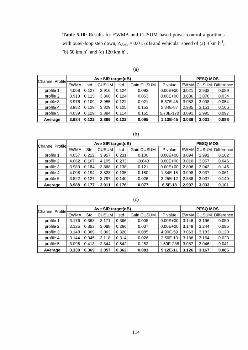
114



(b) 50 km h-1 and (c) 120 km h-1.

(a)

Channel Profile Ave SIR target(dB) PESQ MOS EWMA std CUSUM std Gain CUSUM P value EWMA CUSUM Difference


(b)

Channel Profile Ave SIR target(dB) PESQ MOS EWMA Std CUSUM std Gain CUSUM P value EWMA CUSUM Difference

profile 1 4.057 0.212 3.957 0.231 0.100 0.00E+00 3.094 2.992 0.102 profile 2 4.062 0.167 4.105 0.233 -0.043 0.00E+00 3.010 3.057 0.046 profile 3 3.989 0.184 3.868 0.138 0.121 0.00E+00 2.896 3.042 0.146 profile 4 4.008 0.194 3.828 0.135 0.180 1.34E-15 3.098 3.037 0.061 profile 5 3.822 0.127 3.797 0.140 0.026 3.25E-12 2.888 3.037 0.149 Average 3.988 0.177 3.911 0.176 0.077 6.5E-13 2.997 3.033 0.101

(c)



115



(b) 50 km h-1 and (c) 120 km h-1.

(a)


EWMA std CUSUM std Gain CUSUM P value EWMA CUSUM Difference profile 1 3.965 0.207 3.944 0.211 0.021 8.36E-04 3.037 3.076 0.039 profile 2 3.934 0.248 3.984 0.238 -0.050 0.00E+00 3.201 3.240 0.039 profile 3 3.999 0.171 3.906 0.222 0.093 0.00E+00 3.141 3.100 0.041 profile 4 3.964 0.254 3.944 0.252 0.020 2.76E-78 3.226 3.178 0.049 profile 5 4.007 0.157 3.918 0.238 0.089 0.00E+00 3.116 3.136 0.020 Average 3.974 0.207 3.939 0.232 0.035 1.67E-04 3.144 3.146 0.038

(b)


profile 1 3.852 0.187 3.766 0.284 0.086 8.36E-04 3.049 3.055 0.006 profile 2 3.808 0.227 3.825 0.378 -0.017 2.80E-23 3.006 3.055 0.049 profile 3 3.912 0.230 3.933 0.357 -0.021 0.00E+00 2.944 3.018 0.074 profile 4 3.982 0.198 3.835 0.304 0.147 0.00E+00 3.173 3.210 0.036 profile 5 3.863 0.252 3.871 0.355 -0.008 2.56E-43 2.948 2.932 0.016 Average 3.883 0.219 3.846 0.336 0.037 1.67E-04 3.024 3.054 0.036

(c)

Channel Profile

Ave SIR target(dB) PESQ MOS EWMA Std CUSUM std Gain CUSUM P value EWMA CUSUM Difference

profile 1 2.988 0.411 2.749 0.513 0.239 1.01E-29 3.004 3.151 0.147 profile 2 2.954 0.309 2.939 0.332 0.015 0.00E+00 3.181 3.219 0.037 profile 3 2.981 0.311 2.812 0.435 0.169 3.20E-77 3.096 3.083 0.013 profile 4 3.001 0.397 2.808 0.338 0.193 2.56E-56 3.014 3.135 0.121 profile 5 2.935 0.310 2.794 0.339 0.141 5.70E-124 3.114 3.152 0.038 Average 2.972 0.348 2.820 0.391 0.151 2.02E-30 3.082 3.148 0.071

116

A summary of ensemble averages for the outer-loop step sizes of 0.01, 0.005,

0.015 and 0.02 dB of EWMA based compared to conventional power control algorithm

are given in Table 5.12(a)-(c) respectively.

Table 5.12: Result for Conventional and EWMA based power control

algorithms for all simulated outer loop step sizes and vehicular speed of (a) (a) 3

km h-1, (b) 50 km h-1 and (c) 120 km h-1.

(a)

Step Sizes (dB)


Conv Std EWMA std Gain EWMA P value Conv EWMA Difference 0.005 4.070 0.105 3.000 0.121 1.070 4.30E-12 3.145 3.145 0.069 0.010 4.078 0.107 3.868 0.119 0.210 3.12E-24 3.170 3.170 0.103

0.015 4.051 0.149 3.889 0.122 0.162 7.12E-18 3.155 3.155 0.124

0.020 4.106 0.192 3.939 0.232 0.167 9.08E-13 3.208 3.208 0.062

(b)

Step Sizes (dB)


Conv Std EWMA std Gain EWMA P value Conv EWMA Difference 0.005 4.167 0.082 4.026 0.113 0.141 5.74E-14 3.109 3.109 0.085

0.010 4.251 0.128 4.008 0.131 0.243 1.60E-25 3.109 3.109 0.064

0.015 4.289 0.174 3.988 0.177 0.301 7.30E-19 3.141 3.141 0.108

0.020 4.287 0.220 3.883 0.219 0.404 3.30E-38 3.176 3.176 0.123

(c)

Step Sizes (dB)


Conv Std EWMA std Gain EWMA P value Conv EWMA Difference 0.005 3.640 0.186 3.571 0.216 0.069 4.23E-38 3.426 3.426 0.114

0.010 3.427 0.275 3.309 0.276 0.118 8.48E-33 3.333 3.333 0.111

0.015 3.294 0.314 3.138 0.369 0.156 9.16E-50 3.276 3.276 0.110

0.020 3.260 0.312 2.972 0.348 0.288 6.90E-28 3.270 3.270 0.122

117

A summary of ensemble averages for the outer-loop step sizes of 0.01, 0.005,

0.015 and 0.02 dB are given in Table 5.13(a)-(c) respectively.

Table 5.13: Result for EWMA and CUSUM based power control algorithms for

all simulated outer loop step sizes and vehicular speed of (a) (a) 3 km h-1, (b) 50

km h-1 and (c) 120 km h-1.

(a)

Step Sizes (dB)


EWMA Std CUSUM std Gain CUSUM P value EWMA CUSUM Difference 0.005 3.992 0.144 3.894 0.121 0.098 5.14E-06 3.075 3.077 0.054 0.010 3.978 0.183 3.868 0.119 0.110 6.62E-13 3.057 3.066 0.068

0.015 3.984 0.122 3.889 0.122 0.095 1.13E-45 3.039 3.031 0.088

0.020 3.974 0.207 3.939 0.232 0.035 1.67E-04 3.144 3.146 0.038

(b)

Step Sizes (dB)


EWMA Std CUSUM std Gain CUSUM P value EWMA CUSUM Difference 0.005 4.026 0.113 3.985 0.140 0.041 1.21E-19 3.040 3.024 0.051

0.010 4.008 0.131 3.813 0.129 0.196 7.78E-37 3.035 3.045 0.089

0.015 3.988 0.177 3.911 0.176 0.077 6.50E-13 2.997 3.033 0.101

0.020 3.883 0.219 3.846 0.336 0.037 1.67E-04 3.024 3.054 0.036

(c)

Step Sizes (dB)


EWMA Std CUSUM Std Gain CUSUM P value EWMA CUSUM Difference 0.005 3.571 0.261 3.523 0.247 0.048 3.14E-17 3.327 3.312 0.046 0.010 3.309 0.276 3.169 0.321 0.140 3.08E-05 3.217 3.222 0.059

0.015 3.138 0.369 3.057 0.362 0.081 5.12E-11 3.126 3.167 0.066

0.020 2.972 0.348 2.820 0.391 0.151 2.02E-30 3.082 3.148 0.071

118

A set of representative curves comparing the performance of conventional,

EWMA based and CUSUM based outer-loop power control algorithms for vehicular

speeds of 3 km h-1, 50 km h-1, and 120 km h-1 respectively, are shown in Figure 5.7(a)-

(c) respectively. Since the same results are applied, the figure is similar to Figure 4.11

except there is an addition of a EWMA curve for the comparison. In each case,

shadowing profile and SIR targets for the three algorithms are shown. The CRC flag

indicated the frame erasure. Note that, like conventional and CUSUM, EWMA based

technique also depends on CRC flags as well as the EWMA threshold in controlling

perceptual speech quality. It can be observed from Figure 5.7(a)-(c) that the SIR target

for all algorithms was increased whenever the corresponding CRC flag indicated the

frame erasure. However, there were situations when the frame erasures occurred but the

SIR target for EWMA and CUSUM based techniques was not increased giving rise to

observed gaps between the SIR targets in the three algorithms in Figure 5.7(a)-(c). The

average area of the gap corresponds to the gain achieved through a CUSUM based

algorithm over its SPC counterpart, EWMA and also the gain achieved through

conventional algorithm over EWMA The set of curves corresponding to the best

scenario, which resulted in the highest SIR target gain of CUSUM over EWMA, are

shown in Figure 5.8(a)-(c). In this case, at the given step size of 0.01 dB, SIR target

gains 0.039, 0.268 and 0.190 dB for vehicular speeds of 3 km h-1,50 km h-1, and 120 km

h-1, respectively.

119

0 5 10 15 20 25 30 35 40-25

-20

-15

-10

-5

0

5

10

15

20

25

Time (sec)

Am

plitu

de (

dB

)

Fla

g

Conventional SIR Targets (dB)CUSUM based SIR Targets (dB)EWMA based SIR Targets (dB)Shadowing Profile (dB)CRC Flag (Conventional System)CRC Flag (CUSUM based System)CRC Flag (EWMA based System)

Average SIR Targets (dB): Conventional =4.022, CUSUM = 3.957, EWMA =3.969

(a)

120

0 5 10 15 20 25 30 35 40-25

-20

-15

-10

-5

0

5

10

15

20

25

Time (sec)

Am

plitu

de (

dB

)

Fla

g



(b)

121

0 5 10 15 20 25 30 35 40-25

-20

-15

-10

-5

0

5

10

15

20

25

Time (sec)

Am

plitu

de (

dB

)

Fla

g



(c)

Figure 5.7: Performance comparison of Conventional, CUSUM based and

EWMA based power control (shadowing profile 5 and ∆ = 0.005 dB): (a) 3 km

h-1 , (b) 50 km h-1 and (c) 120 km h-1.

122

0 5 10 15 20 25 30 35 40-25

-20

-15

-10

-5

0

5

10

15

20

25

Time (sec)

Am

plitu

de (

dB

)

Fla

g

Conventional SIR Targets (dB) CUSUM based SIR Targets (dB)EWMA based SIR Targets (dB)Shadowing Profile (dB)CRC Flag (Conventional System)CRC Flag (CUSUM based System)CRC Flag (EWMA based System)


(a)

123

0 5 10 15 20 25 30 35 40-25

-20

-15

-10

-5

0

5

10

15

20

25

Time (sec)

Am

plitu

de (

dB

)

Fla

g



(b)

124

0 5 10 15 20 25 30 35 40-25

-20

-15

-10

-5

0

5

10

15

20

25

Time (sec)

Am

plitu

de (

dB

)

Fla

g



(c)

Figure 5.8: Performance comparison of Conventional, CUSUM based and

EWMA based power control (shadowing profile 1 and ∆ = 0.01 dB): (a) 3 km h-

1 , (b) 50 km h-1 and (c) 120 km h-1.

125

5.3 Summary

Based on data distribution with the application of EWMA and CUSUM analysis, it

shows that CUSUM is slightly more sensitive for the normal distribution data.

However, for non normal data distribution, EWMA shows more sensitivity than

CUSUM. It is also observed that the EWMA has a tendency to be more sensitive with a

larger shift of the distribution. Since ( )log FDn has the normal distribution (FD

Analysis at Section 4.1), applying CUSUM for controlling the transmitter parameter in

the UMTS system is more appropriate than EWMA. Furthermore, based on the

comparison analysis in this chapter it was shown that CUSUM based power control

reduced the average SIR target by up to 5% relative to EWMA based power control

technique. It is noted that applying this new parameter to both EWMA and CUSUM

schemes in a mobile communication system will allow faster action at the transmitter to

control the quality of the speech signals as required by the end users. Hence, it will help

the providers in optimizing the network resources.

The performance of both EWMA based and CUSUM power controls was

compared by computer simulations using a comprehensive set of parameters. These

parameters were the step size of the outer loop power control, vehicular speed and

channel shadowing profile. Both algorithms are better than conventional in term of SIR

target reduction while at the same time providing adequate perceptual quality to the end

users. The simulation results showed that the EWMA based power control reducing the

average SIR target by up to 9 % relative to the conventional based algorithm.

126

CHAPTER 6

CONCLUSIONS Mobile communication system usage has expanded over the years. Mobile phones for

example, have become a necessary item rather than an accessory. Therefore the demand

for good quality systems including speech quality is getting higher. Mobile

communication system providers compete among themselves to offer a better QoS to

the customers and at the same time they can gain financial benefits as well as avoiding a

energy wastage. From an end user’s point of view, they are willing to have a good

quality of QoS while making it cost effective.

Hence, it has inspired researchers to find a method of decreasing the energy

usage while providing an adequate QoS to the customer. In achieving this, the system

which can control the resources at the transmitter such as power control and speech

codec rate control needs to be constructed. Consequently, over the years, power control

has received considerable attention and many good power control algorithms have been

proposed. However most of the proposed algorithms measure speech quality indirectly

based on some channel quality metric such as SIR, BER, and FER. It is agreed by many

researchers that these parameters are actually measures of the quality of received radio

signals, or integrity of the detected bits or frames but not the speech quality as perceived

by the end user. Employment of these inaccurate channel quality metrics will result in

inefficiency in power control algorithms. In this case, at times, more than adequate

quality is provided at the expense of network capacity, while at other times a connection

is considered technically successful but the quality of speech may be poor.

Therefore, to avoid inefficiencies in controlling functions such as power control

and speech codec rate at the transmitter, the more reliable speech quality measures must

be used. Indeed the most reliable speech quality measure should come from the end

user. Hence, the control algorithm based on a human auditory system should be

designed to have efficient control of system resources. As such, among the various

reliable perceptual speech quality metrics, a state of the art method for referenced

objective speech quality measure, PESQ, has an advantage over previously referenced

objective speech quality measures to be employed as the perceptual speech quality

metric in controlling mobile system resources.

A power control algorithm based on PESQ was applied by researchers into the

UMTS system. It was proved that this algorithm is better than the conventional

127

algorithm of UTMS in saving system resources while catering for customers with a

satisfactory QoS. However, the smallest period that PESQ can evaluate speech quality

is 320 ms, which is too long for effective control of quality in networks.

In this thesis, FD which is subtracted from PESQ is proposed to replace a non-

perceptual metric such as FER in mobile radio systems. The FD is calculated every 16

ms and is suitable for control purposes. In order to control functions at the transmitter

such as speech codec rate and power based on FD distribution which is ( )log FDn , an

SPC tool which is novel in mobile communication systems is applied. CUSUM and

EWMA techniques have been applied to UMTS and their effectiveness in better

addressing the aforementioned trade-off between radio resources, and speech quality

has been shown by computer simulation as well as analysis. The major findings and

contributions of this thesis together with possible extensions of it are summarized as

follows.

6.1 Summary of Major Findings and Contributions

In this thesis, ( )log FDn has been proposed for use as a perceptual metric to replace

non-perceptual measures such as SIR, BER and FER. The PESQ is a function of FD.

Specifically FD represents perceptual degradation of each frame of speech. The analysis

of FD in chapter 4 shows that ( )log FDn has a normal distribution where the mean of the

distribution increases with the degradation of perceptual speech quality and vice versa.

The FD analysis suggests that transmission parameters such as power should not be

adapted on a frame by frame basis as is the current practice. Current practices lead to

inefficient utilization of resources and possible unsatisfactory perceptual speech quality.

In maintaining a certain level of end user perceptual quality, what is needed is to detect

a shift in the distribution of ( )log FDn and take steps to rectify that such as controlled

the transmission power, channel coding or speech codec rate.

A CUSUM based technique was proposed as a novel technique for controlling

the speech codec rate and control power in mobile communication systems. In chapter

4, Section 4.2, a CUSUM based technique is applied for controlling the speech codec

rate for UMTS. The CUSUM based technique which employed log( )nFD as the

perceptual speech quality parameter allows faster action at the transmitter to control the

quality of the speech signals as required by end users. Hence, the non-perceptual speech

parameter such as FER can be replaced with log( )nFD .

128

In Chapter 4, Section 4.3, the CUSUM based technique was applied for

controlling the transmission power at the transmitter for UMTS. The UMTS outer loop

power control was modified to employ the CUSUM based technique. Instead of

increasing the SIR target every time a frame error occurred, the perceptual importance

of the erroneous frame was determined by the CUSUM based technique before the

process proceeded. If the erroneous frame was of sufficient perceptual importance, only

then was the SIR target increase allowed, otherwise, the SIR target was decreased. A

comparison of the performance of CUSUM based and FER based outer loop power

control algorithms through simulations using a comprehensive set of parameters was

carried out, and the simulation results show the CUSUM based power control achieves

adequate speech quality while reducing the average SIR target by up to 13% relative to

the conventional algorithm.

The CUSUM based power control algorithm enabled the trade-off of average

perceptual quality with average SIR target in a more controlled manner. This cannot be

achieved with conventional power control of UMTS. This inefficiency of the

conventional power control would not allow accurate control of speech quality. This is

mainly due to inaccuracy of the FER as a non-perceptual quality metric in representing

speech quality. The conventional power control algorithm tried to keep FER within a

specified range that would guarantee good quality in all situations. This, however, at

times meant that more than necessary perceptual quality was provided.

The application of a CUSUM based technique in power control in UMTS

required feedback of FEP, every 20 ms, from the receiver end of the communication

link to the transmitter. It implies a requirement of the feedback channel for this purpose.

Therefore, FEP could be included in the feedback channels already available.

In chapter 5, the comparison analysis between EWMA and CUSUM based

techniques is analysed. Section 5.1, the response of EWMA and CUSUM based

techniques towards data distribution is observed and analysed showing that in our case,

the EWMA technique has a better response with the data which does not have normal

distribution compared to a CUSUM technique. On the other hand, the CUSUM

technique has a better response with normal distribution data compared to a EWMA

technique. The analysis also implies that EWMA is more sensitive with a larger shift of

data where EWMA is more sensitive with data which does not have a normal

distribution.

In Section 5.2, the performance comparison between EWMA based and

CUSUM based power control algorithms is presented through simulations. It is shown

129

that both EWMA and CUSUM algorithms reduce the average SIR target compared to

conventional algorithm where EWMA based power control achieves up to 9% relative

to a conventional algorithm. However, CUSUM based power control achieves adequate

speech quality while reducing the average SIR target slightly by up to 5% relative to the

EWMA based algorithm. It shows that the CUSUM has more sensitivity towards

( )log FDn distributions which have a normal distribution. Generally, the perceptual

quality delivered by conventional power control is slightly higher than

CUSUM/EWMA based algorithms. This is due to the ability of the perceptual

algorithms to trade-off transmit power with perceptual quality in a more controlled

manner while still providing adequate quality to the users. Furthermore, it should be

noted that the MOS differences between perceptual algorithms and conventional

algorithms are hardly perceptible (less than 0.2 MOS). Therefore, we could say, all the

algorithms deliver adequate perceptual qualities but with a different cost in term of

average SIR target levels.

6.2 Suggestions for Future Work

The benefits of applying the SPC in power control of mobile communication systems is

shown in this thesis to be mainly as saving precious system resources such as

transmitter power as well as providing the adequate speech quality to end users.

However, since the thesis is mostly based on numerical simulations, more theoretical

analysis will improve the balance between numerical and theoretical analysis in the

thesis. Furthermore, there are a number of extensions to this work that could be

considered for future research in methodology, which potentially will improve the

performance of SPC based techniques. The suggested extensions are as follows:

Pre-emptive perceptual power control

The proposed perceptual power control algorithms are reactive since they wait for a

frame error to occur and depend on the perceptual importance of the erroneous frame

reaction in an attempt to keep the overall perceptual quality within a prescribed range.

In the situation where the received frames on which quality measure were made, they

were severely corrupted to such an extent as to degrade the overall perceived speech

quality; significantly, the system could not do much to improve the speech quality.

However, if there are pre-emptive measures which predict the perceptual significance of

frames before they are transmitted and protect them accordingly, it can avoid the

130

particular situation. The frame can be protected in many ways such as unequal error

protection, unequal signal power allocation for the frames, etc.

Simplification of PESQ

PESQ is designed for a wide range of network conditions and error types as well as

applications. For a specific application such as in a mobile communication system, the

PESQ algorithm could be simplified for the application without losing much accuracy.

There are functional blocks in PESQ, such as input filtering, which should be studied

and justified. The simpler the PESQ algorithm, the smaller the memory space required

for implementation of SPC based algorithms on mobile and base stations. With less

blocks in PESQ, the execution time of algorithm will be faster.

131

APPENDIX

ITU Speech Files TABLE A: ITU Speech files used for FD analysis for PESQ MOS 3.0

Speaker gender ITU File name Speaker gender ITU File name

Female O_0F01L84 Male O_M02L3C

Female O_0F02LBA Male O_M02L2D

Female O_0F02L8C Male O_M02L3A

Female O_0F02L8E Male O_M02L3E

Female O_0F02L8F Male O_M02L4A TABLE B: ITU Speech files used for FD analysis for PESQ MOS 3.1


Female O_0F01L5A Male O_M01L02

Female O_0F02L5B Male O_M01L2B

Female O_0F02L5D Male O_M01L04

Female O_0F02L6C Male O_M01L07

Female O_0F02L7B Male O_M01L08 TABLE C: ITU Speech files used for FD analysis for PESQ MOS 3.2



Female O_0F01L5E Male O_M01L08

Female O_0F01L6B Male O_M01L12



132

TABLE D: ITU Speech files used for FD analysis for PESQ MOS 3.3


Female O_0F01L6A Male O_M01L0F

Female O_0F01L7A Male O_M01L09


Female O_0F01L60 Male O_M01L13

Female O_0F01L61 Male O_M01L14 TABLE E: ITU Speech files used for FD analysis for PESQ MOS 3.4


Female O_0F01L5F Male O_M01L0A

Female O_0F01L6F Male O_M01L0B

Female O_0F01L7A Male O_M01L0E

Female O_0F01L61 Male O_M01L1F

Female O_0F01L67 Male O_M01L2B TABLE F: ITU Speech files used for FD analysis for PESQ MOS 3.5


Female O_0F01L5F Male O_M01L0C

Female O_0F01L6A Male O_M01L0D

Female O_0F01L7A Male O_M01L0E

Female O_0F01L61 Male O_M01L1A

Female O_0F01L68 Male O_M01L1B

133

BIBLIOGRAPHY

[1] Objective Quality Measurement of Telephone Band (300-34000Hz) Speech

Codecs, ITU-T Recommendation P.861, August 1996.

[2] J. G. B. Antony W.Rix1, Michael P. Hollier1 and Andries P. Hekstra2,

"Perceptual Evaluation of Speech Quality (PESQ) - A New Method for Speech

Quality Assessment of Telephone Networks and Codecs," in Proceeding IEEE

International Conference on Acoustics, Speech, and Signal Processing (ICASSP

'01) Salt Lake City, Utah, USA, May 2001, pp. 749-752.

[3] Behrooz Rohani and H. J. Zepernick, "Application of a Perceptual Speech

Quality Metric in Power Control of UTMS," in 2nd ACM International

Workshop on Quality of Service & Security for Wireless and Mobile Networks

(Q2sWinet'06), Torremolinos,(Malaga), Spain, Oct 2006, pp. 87-94.

[4] Behrooz Rohani, et al., "Application of a Perceptual Speech Quality Metric for

Link Adaptation in Wireless Systems," in 1st International Symposium on

Wireless Communication Systems, Mauritius, Sept 2004, pp. 260-264.

[5] S. Mohammed, et al., "Integrating Network Measurements and Speech Quality

Subjective Scores for Control Purposes," in 20th Annual Joint Conference of the

IEEE Computer and Communication Societies INFOCOM 2001, Anchorage,

Alaska, USA, April 2001, pp. 641-649.

[6] W.H. Woodwall and D. C. Montgomery, "Research Issues and Ideas in

Statistical Process Control," Journal of Quality Technology, vol. 31, pp. 376-

386, 1999.

[7] E.S Page, "Continuous Inspection Schemes," Biometrika, vol. 41, pp. 100-115,

1954.

134

[8] Perceptual Evaluation of Speech Quality (PESQ), An Objective Method for End-

to-End Speech Quality Assessment of Narrow Band Telephone Networks and

Speech Codecs, ITU-T Recommendation P.862, Feb 2001.

[9] Evaluation of Speech Quality (PESQ), and Objective Method for End-to end

Speech Quality Assessment of Narrow-band Telephone Networks and Speech

Codecs, ITU-T Recommendation P.862, Feb. 2001.

[10] D. M. Novakovic and M. L. Dukic, "Evolution of the Power Control Techniques

for DS-CDMA Toward 3G Wireless Communication Systems," IEEE

Communications Surveys & Tutorials, vol. 3, pp. 2-15, 2000.

[11] S. Nanda, et al., "Adaptation Techniques in Wireless Packet Data Services,"

IEEE Comm. Magazine, pp. 54-64, Jan 2000.

[12] S. Pennock, "Accuracy of the Perceptual Evaluation of Speech Quality (PESQ)

Algorithm," in Proc. of MESAQIN - The Measurement of Speech and Audion

Quality in Networks, Prague, Czech Republic, Jan 2002.

[13] H. Hosseini, et al., "Objective Characterization of Voice Service Quality in

Wideband CDMA," in IEEE VTC Conference, Rhodes, Greece, May 2001, pp.

2708-2711.

[14] A. W. Rix, "Perceptual Speech Quality Assessment - A Review," in IEEE

Conference on Acoustics, Speech, and Signal Processing, Montreal, Quebec,

Canada, May 2004, pp. 1056-1059.

[15] A. W. Rix, et al., "Objective Assessment of speech and Audio Quality -

Technology and Applications," IEEE Transactions on Audio, Speech, and

Language Processing, vol. 14, pp. 1890-1901, 2006.

[16] E. Zwicker and H. Fastl, Psychoacoustics: Facts and Models, Second Updated

ed. Heidelberg: Springer, 1999.

135

[17] T. Dimauro. (2002, Spring). Physics of Speech, Hearing, and Sound. Available:

http://sdsu-physics.org/physics201/physics201.html

[18] J. G. W. Bernstein and A. J. Oxenham, "The Relationship Between Frequency

Selectivity and Pitch Discrimination: Effects of Stimulus Level," The Journal of

the Acoustical Society of America, vol. 120, pp. 3916-3928, 2006.

[19] K. Suresh, et al., "Direct MDCT Domain Psychoacoustic Modeling," in

Symposium on Signal Processing and Information Technology, 2007 IEEE

International Cairo, Egypt, Dec 2007, pp. 742-747.

[20] H. Fletcher, "Auditory Patterns," Reviews of Modern Physics, vol. 12, p. 47,

1940.

[21] J. V. Tobias, Foundation of Modern Auditory Theory, vol. 1: Academic Press,

1970.

[22] M. Bosi and R. E. Goldberg, Introduction to Digital Audio Coding and

Standards. Boston: Kluwer Academic Publishers, December 2002.

[23] F. Harvey, "The Relation Between Loudness and Masking," The Journal of the

Acoustical Society of America, vol. 7, p. 238, 1936.

[24] M. Krasner, "The Critical Band Coder--Digital Encoding of Speech Signals

Based on the Perceptual Requirements of the Auditory System," in IEEE

International Conference on Acoustics, Speech, and Signal Processing (ICASSP

'80), Denver, Colorado, USA, April 1980, pp. 327-331.

[25] Methods for Subjective Determination of Transmission Quality, ITU-R

Rocemmendation P.800, August 1996.

[26] M. Karjalainen, "A New Auditory Model for the Evaluation of Sound Quality of

Audio Systems," in IEEE International Conference on Acoustics, Speech, and

http://sdsu-physics.org/physics201/physics201.html

136

Signal Processing (ICASSP '85), Tampa, Florida, USA, March 1985, pp. 608-

611.

[27] Schuyler R. Quackenbush, et al., Objective Measures of Speech Quality. New

York: Prentice Hall, 1998.

[28] S. Voran, "Objective Estimation of Perceived Speech Quality. I. Development of

the Measuring Normalizing Block Technique," IEEE Transactions on Speech

and Audio Processing, vol. 7, pp. 371-382, 1999.

[29] S. Wang, et al., "An Objective Measure for Predicting Subjective Quality of

Speech Coders," IEEE Journal on Selected Areas in Communications, vol. 10,

pp. 819-829, June 1992.

[30] R. Mannel, "The Perceptual and Auditory Implications of Parametric Scaling in

Synthetic Speech," Ph.D, Dept of Linguistic, Macquarie University, Sydney,

1994.

[31] J. O. Smith, III and J. S. Abel, "Bark and ERB Bilinear Transforms," IEEE

Transactions on Speech and Audio Processing, vol. 7, pp. 697-708, 1999.

[32] M. P. Hollier, et al., "Error Activity and Error Entropy as a Measure of

Psychoacoustic Significance in the Perceptual Domain," IEEE Proceedings on

Vision, Image and Signal Processing, vol. 141, pp. 203-208, 1994.

[33] J.G. Beereds and J. A. Stemerdink, "A Perceptual Audio Quality Measure Based

on a Psychoacoustic Sound Representation," Journal of the Audio Engineering

Society, vol. 40, pp. 963-974, Dec 1992.

[34] B. Pailard, et al., "PERCEVAL: Perceptual Evaluation of the Quality of Audio

Signals," Journal of the Audio Engineering Society, vol. 40, pp. 21-31, Jan 1992.

[35] C. Colomes, et al., "A Perceptual Model Applied to Audio Bit-Rate Reduction,"

Journal of the Audio Engineering Society, vol. 43, pp. 223-240, April 1995.

137

[36] J.G. Beerends and J. A. Stemerdink, "A Perceptual Speech Quality Measure

Based on a Psycho Sound Reperesentation," Journal of the Audio Engineering

Society, vol. 42, pp. 115-123, November 1994.

[37] A. W. Rix and M. P. Hollier, "The Perceptual Analysis Measurement System for

Robust End-to-End Speech Quality Assessment," in Proceedings IEEE

International Conference on Acoustics, Speech, and Signal Processing ( ICASSP

'00), Istanbul, Turkey, June 2000, pp. 1515-1518

[38] The E-model, a Computational Model for Use in Transmission Planning, ITU-T

Recommendation G. 107, July 2002.

[39] L. Carvalho, et al., "An E-model Implementation for Speech Quality Evaluation

in VoIP Systems," in Proceedings 10th IEEE Symposium on Computers and

Communications ( ISCC 2005) Cartegena, Spain, June 2005, pp. 933-938.

[40] D. S. Kim, "ANIQUE: An Auditory Model for Single-Ended Speech Quality

Estimation," IEEE Transactions on Speech and Audio Processing, vol. 13, pp.

821-831, 2005.

[41] K. Doh-Suk and A. Tarraf, "Perceptual Model for Non-intrusive Speech Quality

Assessment," in Proceedings IEEE International Conference on Acoustics,

Speech, and Signal Processing (ICASSP '04), 2004, pp. iii-1060-3.

[42] Single-ended Method for Objective Speech Quality Assessement in Narrow-band

Telephony Applications, ITU-T Recommendation P.563, May 2004.

[43] A. P. Markopoulou, et al., "Assessment of VoIP Quality Over Internet

Backbones," in Proceedings Twenty-First Annual Joint Conference of the IEEE

Computer and Communications Societies (INFOCOM 2002), New York, USA,

June 2002, pp. 150-159.

138

[44] A. Takahashi, et al., "Objective Assessment Methodology for Estimating

Conversational Quality in VoIP," IEEE Transactions onAudio, Speech, and

Language Processing, vol. 14, pp. 1984-1993, 2006.

[45] S. Moller and G. Berger, "Describing Telephone Speech Codec Quality

Degradations by Means of Impairment Factors," Journal of the Audio

Engineering Society, vol. 50, pp. 667-680, September 2002.

[46] S. C. Chen, et al., "On Distributed Power Control for Radio Networks," in IEEE

International Conference on Communications (ICC '94) 'Serving Humanity

Through Communications', New Orleans, Louisiana, USA, May 1994, pp. 1281-

1285

[47] Harri Holma and A. Toskala, WCDMA for UMTS-HSPA Evolution and LTE, 4

ed. Chichester: John Wiley & Sons Ltd, 2007.

[48] W. Qiang, "Performance of Optimum Transmitter Power Control in CDMA

Cellular Mobile Systems," IEEE Transactions on Vehicular Technology, vol. 48,

pp. 571-575, 1999.

[49] W. Qiang, "Optimum Transmitter Power Control in Cellular Systems with

Heterogeneous SIR Thresholds," IEEE Transactions on Vehicular Technology,

vol. 49, pp. 1424-1429, 2000.

[50] R. Prasad and T. Ojanpera, "A Survey on CDMA: Evolution Towards Wideband

CDMA," in Proceedings IEEE 5th International Symposium on Spread

Spectrum Techniques and Applications, Sun City, South Africa, Sept 1998, pp.

323-331.

[51] A. Sampath, et al., "On Setting Reverse Link Target SIR in a CDMA System,"

in IEEE 47th Vehicular Technology Conference, Pheonix, Arizona, USA, May

1997, pp. 929-933.

139

[52] M. P. J. Baker and T. J. Mouslsley, "Power control in UMTS Release '99," in

First International Conference on (Conf. Publ. No. 471) 3G Mobile

Communication Technologies, London, UK, March 2000, pp. 36-40.

[53] R. Tanner and J. Woodards, WCDMA Requirement and Practical Design, 3rd

ed.: Chichester : John Wiley and Sons, 2004.

[54] H. Axen, "Power Control in Cellular Mobile Telephone Systems (in Swedish),"

Erricson Radio Systems, 1990.

[55] H. Axen, "Uplink C/I as Control Parameter for Mobile Station Power Control (in

Swedish)," Erricson Radio Systems, 1990.

[56] J. Zander, "Distributed Cochannel Interference Control in Cellular Radio

Systems," IEEE Transactions on Vehicular Technology, vol. 41, pp. 305-311,

1992.

[57] J. Zander, "Performance of Optimum Transmitter Power Control in Cellular

Radio Systems," IEEE Transactions on Vehicular Technology, vol. 41, pp. 57-

62, 1992.

[58] G. J. Foschini and Z. Miljanic, "A Simple Distributed Autonomous Power

Control Algorithm and Its Convergence," IEEE Transactions on Vehicular

Technology, vol. 42, pp. 641-646, 1993.

[59] S. A. Grandhi, et al., "Distributed Power Control in Cellular Radio Systems,"

IEEE Transactions on Communications, vol. 42, pp. 226-228, 1994.

[60] S. A. Grandhi and J. Zander, "Constrained Power Control in Cellular Radio

Systems," in IEEE 44th Vehicular Technology Conference, Stockholm, Sweden,

June 1994, pp. 824-828.

140

[61] F. Berggren, et al., "A Generalized Algorithm for Constrained Power Control

with Capability of Temporary Removal," IEEE Transactions on Vehicular


[62] M. Rasti, et al., "Improved Distributed Power Control Algorithms with Gradual

Removal in Wireless Networks," in 14th European Wireless Conference (EW

2008) Prague, Czech Republic, June 2008, pp. 1-5.

[63] M. Rasti, et al., "A Distributed and Efficient Power Control Algorithm for

Wireless Networks," in IEEE 19th International Symposium onPersonal, Indoor

and Mobile Radio Communications (PIMRC 2008), Cannes, France, Sept 2008,

pp. 1-6.

[64] V. Vanghi, et al., The cdma2000 Systems for Mobile Communications. New

Jersey: Prentice Hall, 2004.

[65] J. P. Castro, The UMTS Network and Radio Access Technology: Air Interface

Techniques for Future Mobile Systems. Chichester: John Wiley and Sons, 2001.

[66] A. M. Viterbi and A. J. Viterbi, "Erlang Capacity of a Power Controlled CDMA

System," in Proceedings IEEE International Symposium on Information Theory,

San Antonio, Texas, USA, Jan 1993, pp. 254-254.

[67] Technical Specification Group Access Nertowrk; Physical Layer procedures

(FDD) (Release 6), V 6.2.0, June 2004.

[68] D. C. Montgomery, Introduction to Statistical Quality Control. New York,

1996.

[69] George Box and A. Luceno, Statistical Control by Monitoring and Feedback

Adjustment: John Wiley & Son, 1997.

[70] A. Hossain, et al., "Statistical Process Control of an Industrial Process in Real

Time," IEEE Transactions on Industry Applications, vol. 32, pp. 243-249, 1996.

141

[71] A. Cinar and C. Undey, "Statistical Process and Controller Performance

Monitoring. A Tutorial on Current Methods and Future Directions," in

Proceedings of the American Control Conference San Diego, California, USA,

June 1999, pp. 2625-2639.

[72] Ming T. Tham. (1997, An Introduction to SPC. Available:

http://lorien.ncl.ac.uk/ming/spc/spc0.htm

[73] W. A. Shewhart, "Quality Control Charts," Bell System Technical Journal, vol.

5, pp. 593-602, 1926.

[74] M. E. Camargo, et al., "Statistical Quality Control: A Case Study Research," in

4th IEEE International Conference on Management of Innovation and

Technology (ICMIT 2008), Bangkok, Thailand, Sept 2008, pp. 746-750.

[75] R. E. Mohammad Abaii, "Transmission Power Control Using Perceptual Quality

Metrics," in Preceeding on 14th IEEE Personal Indoor and Mobile Radio

Communications (PIMRC 2003), Beijing, China, Sept 2003, pp. 2317-2321.

[76] A.R Prasad, et al., "Perceptual Quality Measurement and Control: Definition,

Application and Performance," in 4th International Symposium on Wireless

Personal Multimedia Communication (WPMC'01), Aalborg, Denmark, Sept

2001, pp. 553-556.

[77] ITU-T Coded-Speech Database, ITU-T Recommendation, February 1998.

[78] Mandatory Speech Codec Speech Processing Functions; Adaptive Multi-rate

(AMR) Speech Codec Frame Structure (Release 6), 3GPP TS 26.101 V6.0.0,

September 2004.

[79] Mandatory Speech Codec Speech Processing Functions; Interface to lu, Uu and

Nb (Release 6), 3GPP TS 26.102 V6.0.0, September 2004.

http://lorien.ncl.ac.uk/ming/spc/spc0.htm

142

[80] B. Rohani and H. J. Zepernick, "An Efficient Method for Perceptual Evaluation

of Speech Quality in UMTS," in Proceedings International Conference on

Multimedia Communications System, Montreal, Canada, Aug 2005, pp. 185-190.

[81] B. Rohani and H. J. Zepernick, "Frame Erasure Pattern Feedback for Real-time

Perceptual Quality Estimation," in Proceedings of the Joint Conference of the

Fourth International Conference on Information, Communications and Signal

Processing and Fourth Pacific Rim Conference on Multimedia, Singapore, Dec

2003, pp. 110-113.

[82] B. Rohani and H. J. Zepernick, "Feedback Method for Real-time Perceptual

Quality Estimation," Electronics Letters, vol. 40, pp. 913-915, 2004.

[83] AMR Speech Codec Frame Structure, 3G TS 26.10, March 2002.

[84] AMR Speech Codec; Error Concealment of Lost Frames, 3G TS 26.091, March

2001.

[85] Ewan and W.D., "When and How to Use Cusum Chart," Technometrics, vol. 5,

pp. 1-22, 1963.

[86] J. M. Lucas, "The Design and Use of V-mask Control Scheme," Journal of

Quality Technology, vol. 8, pp. 1-12, 1976.

[87] F. F. Gan, "Joint Monitoring of Process Mean and Variance Using Exponentially

Weighted Moving Average Control Charts," Technometrics, vol. 37, pp. 446-

453, 1995.

[88] D. M. Hawkins, "Self-Starting Cusum Charts for Location and Scale," Journal

of the Royal Statistical Society. Series D (The Statistician), vol. 36, pp. 299-316,

1987.

[89] W. H. Woodall and B. M. Adams, "The Statistical Design of Cusum Charts,"

Quality Engineering, vol. 5, pp. 559 - 570, 1993.

143

[90] Bissel and A.F., "Cusum Techniques for Quality Control," Applied Statistics,

vol. 18, pp. 1-30, 1969.

[91] W. Zhang and Y. Mei, "A CUSUM Chart Using Absolute Sample Values to

Monitor Process Mean and Variance," in IEEE International Conference on

Industrial Engineering and Engineering Management (IEEM 2009), Hong

Kong, Dec 2009, pp. 414-418.

[92] J. D. Healy, "A Note on Multivariate CUSUM Procedure," Technometrics, vol.

29, pp. 409-412, Nov. 1987.

[93] A. L. Goel and S. M. Wu, "Economically Optimum Design of Cusum Charts,"

Management Science, vol. 19, pp. 1271-1282, 1973.

[94] R. Gerlach, et al., "Diagnostics for Time Series Analysis," Journal of Time

Series Analysis, vol. 20, pp. 309-330, 1999.

[95] G. A. Barnard, "Control Charts and Stochastic Processes," Journal of the Royal

Statistical Society. Series B (Methodological), vol. 21, pp. 239-271, 1959.

[96] J. M. Lucas, "A modified V Mask Control Scheme," Technometrics, vol. 15, pp.

833-847, 1973.

[97] L.A Jones, et al., "The Run Length Distribution of the CUSUM with Estimated

Parameters," Journal of Quality Technology, vol. 36, pp. 95-108, Jan 2004.

[98] Michael J. Cybrynski, et al. (2010, 3 July). Defining the V-Mask for a Two-

Sided Cusum Scheme (Second ed.). Available:

http://www.jmu.edu/docs/sasdoc/sashtml/qc/chap12/sect16.htm

[99] N. L. Johnson, "A Simple Theoretical Approach to Cumulative Sum Control

Charts," Journal of the American Statistical Association, vol. 56, pp. 835-840,

1961.

http://www.jmu.edu/docs/sasdoc/sashtml/qc/chap12/sect16.htm

144

[100] S. W. Roberts, "Control Chart Tests Based on Geometric Moving Averages,"

Technometrics, vol. 42, pp. 97-101, 2000.

[101] H.-Y. Wang, "An EWMA for Monitoring Stationary Autocorrelated Process," in

International Conference on Computational Intelligence and Software

Engineering (CiSE 2009), Wuhan, China, Dec 2009, pp. 1-4.

[102] M. Khoo and A. Atta, "An EWMA Control Chart for Monitoring the Mean of

Skewed Populations Using Weighted Variance," in IEEE International

Conference on Industrial Engineering and Engineering Management (IEEM

2008), Singapore, Dec 2008, pp. 218-223.

[103] D. M. Hawkins, Olwell, David H., Cumulative Sum Charts and Charting for

Quality Improvement. New York: Springer-Verlag, 1998.

[104] G.E. Box, et al., Time Series Analysis: Forecasting and Control: Prentice Hall

PTR, 1994.

[105] M. D.C., et al., Forecasting and Time Series Analysis, 2nd ed. New York:

McGraw-Hill, 1990.

[106] J. S. Hunter, "The Exponetially Weighted Moving Average," Journal of Quality


[107] J. S. Hunter, "A One-point Plot Equaivalent to the Shewhart Chart with Western

Electric Rules," Quality Engineering, vol. 2, pp. 13 - 19, 1989.

[108] "Perceptual Evaluation of Speech Quality (PESQ), An Objective Method for

End-to-End Speech Quality Assessment of Narrow Band Telephone Networks

and Speech Codecs," I.-T. R. P.862, Ed., ed: , 2001.

[109] 3GPP Technical Report 25.101 V4.1.0, "Channel Coding and Multiplexing

Example (Release 4)," June June 2001.

145

[110] Channel Coding and Multiplexing Example (Release 4), 3GPP Technical Report

25.101 V4.1.0, June 2001.

[111] Simon R. Saunders, Antennas and Propagation for Wireless Communication

Systems: Chichester: John Wiley & Sons Ltd, 1999.

[112] User Equipment (UE) Radio Transmission and Reception (FDD) (Release 6),

3GPP Technical Specification 25.101 V6.10.0, Dec 2005.

[113] Guidelines for Evaluation of Radio Transmission Technologies for IMT-2000,

ITU-R Recommendation M.1225, Feb 1977.

[114] W. Jakes, Microwave Mobile Communication: New York: John Wiley and Sons,

1978.

[115] K.S. Gilhousen, et al., "On the Capacity of a Celullar CDMA system," IEEE

Trans. Veh. Technology, vol. 40, pp. 303-312, May 1991.

[116] M.C. Jeruchim, et al., Simulation of Communication Systems, Modeling,

Methodolgy and Techniques, 2nd ed.: New York: Kluwer Academic, 2000.

[117] W. R.Rice, "Analyzing Tables of Statistical Tests," Evolution, vol. 43, pp. 223-

225, Jan 1989.

[118] L. Van Brackle and M. R. Reynolds, "EWMA and CUSUM Control Charts in

the Presence of Correlation," Communications in Statistic-Simulation and

Computation, vol. 26, pp. 979-1008, 1997.

[119] De Vargas V.D.C.C., et al., "Comparative Study of the Performance of the

CUSUM and EWMA Control Charts," Computers and Industrial Engineering,

vol. 46 pp. 707-724, 2004.

Documents

PERCEPTUAL SPEECH CONTROL