PEGASUS: A Peta-Scale Graph Mining System - Implementationand Observations

U KangSCS, Carnegie Mellon University

ukang@cs.cmu.edu

Charalampos E. TsourakakisSCS, Carnegie Mellon University

ctsourak@cs.cmu.edu

Christos FaloutsosSCS, Carnegie Mellon University

christos@cs.cmu.edu

Abstract—In this paper, we describe PEGASUS, an opensource Peta Graph Mining library which performs typicalgraph mining tasks such as computing the diameter of thegraph, computing the radius of each node and finding theconnected components. As the size of graphs reaches severalGiga-, Tera- or Peta-bytes, the necessity for such a librarygrows too. To the best of our knowledge, PEGASUS is the firstsuch library, implemented on the top of the HADOOP platform,the open source version of MAPREDUCE.

Many graph mining operations (PageRank, spectral cluster-ing, diameter estimation, connected components etc.) are es-sentially a repeated matrix-vector multiplication. In thi s paperwe describe a very important primitive for PEGASUS, calledGIM-V (Generalized Iterated Matrix-Vector multiplication).GIM-V is highly optimized, achieving (a) good scale-up on thenumber of available machines (b) linear running time on thenumber of edges, and (c) more than5 times faster performanceover the non-optimized version ofGIM-V.

Our experiments ran on M45, one of the top 50 supercom-puters in the world. We report our findings on several realgraphs, including one of the largest publicly available WebGraphs, thanks to Yahoo!, with ≈ 6,7 billion edges.

Keywords-PEGASUS; graph mining; hadoop

I. I NTRODUCTION

Graphs are ubiquitous: computer networks, social net-works, mobile call networks, the World Wide Web [1],protein regulation networks to name a few.

The large volume of available data, the low cost of storageand the stunning success of online social networks andweb2.0 applications all lead to graphs of unprecedentedsize. Typical graph mining algorithms silently assume thatthe graph fits in the memory of a typical workstation, orat least on a single disk; the above graphs violate theseassumptions, spanning multiple Giga-bytes, and heading toTera- and Peta-bytes of data.

A promising tool is parallelism, and specifically MAPRE-DUCE [2] and its open source version, HADOOP. Basedon HADOOP, here we describe PEGASUS, a graph min-ing package for handling graphs withbillions of nodesand edges. The PEGASUS code and several dataset areat http://www.cs.cmu.edu/∼pegasus. The contributions arethe following:

1) Unification of seemingly different graph mining tasks,via a generalization of matrix-vector multiplication(GIM-V).

2) The careful implementation ofGIM-V, with severaloptimizations, and several graph mining operations(PageRank, Random Walk with Restart(RWR), diame-ter estimation, and connected components). Moreover,the method is linear on the number of edges, and scalesup well with the number of available machines.

3) Performance analysis, pinpointing the most successfulcombination of optimizations, which lead to up to5timesbetter speed than naive implementation.

4) Analysis of large, real graphs, including one of thelargest publicly available graph that was ever analyzed,Yahoo’s web graph.

The rest of the paper is organized as follows. Sec-tion II presents the related work. Section III describes ourframework and explains several graph mining algorithms.Section IV discusses optimizations that allow us to achievesignificantly faster performance in practice. In Section V wepresent timing results and Section VI our findings in realworld, large scale graphs. We conclude in Section VII.

II. BACKGROUND AND RELATED WORK

The related work forms two groups, graph mining, andHADOOP.

Large-Scale Graph Mining.:There are a huge numberof graph mining algorithms, computing communities (eg.,[3], DENGRAPH [4], METIS [5]), subgraph discovery(e.g.,GraphSig [6], [7], [8], [9], gPrune [10], gApprox [11],gSpan [12], Subdue [13], HSIGRAM/VSIGRAM [14],ADI [15], CSV [16]), finding important nodes (e.g., PageR-ank [17] and HITS [18]), computing the number of tri-angles [19], [20], computing the diameter [21], topic de-tection [22], attack detection [23], with too-many-to-listalternatives for each of the above tasks. Most of the previousalgorithms do not scale, at least directly, to several millionsand billions of nodes and edges.

For connected components, there are several algorithms,using Breadth-First Search, Depth-First-Search, “propaga-tion” ([24], [25], [26]), or “contraction” [27] . These worksrely on a shared memory model which limits their ability tohandle large, disk-resident graphs.

MapReduce and Hadoop.:MAPREDUCE is a program-ming framework [2] [28] for processing huge amounts ofunstructured data in a massively parallel way. MAPREDUCE

has two major advantages: (a) the programmer is oblivious

of the details of the data distribution, replication, load bal-ancing etc. and furthermore (b) the programming concept isfamiliar, i.e., the concept of functional programming. Briefly,the programmer needs to provide only two functions, amapand areduce. The typical framework is as follows [29]: (a)the map stage sequentially passes over the input file andoutputs (key, value) pairs; (b) theshufflingstage groups ofall values by key, (c) thereducestage processes the valueswith the same key and outputs the final result.

HADOOP is the open source implementation of MAPRE-DUCE. HADOOP provides the Distributed File System(HDFS) [30] and PIG, a high level language for dataanalysis [31]. Due to its power, simplicity and the factthat building a small cluster is relatively cheap, HADOOP

is a very promising tool for large scale graph miningapplications, something already reflected in academia, see[32]. In addition to PIG, there are several high-level languageand environments for advanced MAPREDUCE-like systems,including SCOPE [33], Sawzall [34], and Sphere [35].

III. PROPOSEDMETHOD

How can we quickly find connected components, diameter,PageRank, node proximities of very large graphs fast? Weshow that, even if they seem unrelated, eventually wecan unify them using theGIM-V primitive, standing forGeneralized Iterative Matrix-Vector multiplication, whichwe describe in the next.

A. Main Idea

GIM-V, or ‘Generalized Iterative Matrix-Vector multipli-cation’ is a generalization of normal matrix-vector multipli-cation. Suppose we have an by n matrix M and a vectorvof sizen. Let mi,j denote the (i, j)-th element ofM . Thenthe usual matrix-vector multiplication is

M × v = v′ wherev′i =∑n

j=1 mi,jvj .

There are three operations in the previous formula, which,if customized separately, will give a surprising number ofuseful graph mining algorithms:

1) combine2: multiply mi,j andvj .2) combineAll: sum n multiplication results for node

i.3) assign: overwrite previous value ofvi with new

result to makev′i.

In GIM-V, let’s define the operator×G, where the threeoperations can be defined arbitrarily. Formally, we have:

v′ = M ×G vwherev′i = assign(vi,combineAlli({xj | j =1..n, andxj =combine2(mi,j, vj)})).

The functions combine2(), combineAll(), andassign() have the following signatures (generalizingthe product, sum and assignment, respectively, that thetraditional matrix-vector multiplication requires):

1) combine2(mi,j, vj) : combinemi,j andvj .

2) combineAlli(x1, ..., xn) : combine all the resultsfrom combine2() for nodei.

3) assign(vi, vnew) : decide how to updatevi withvnew .

The ‘Iterative’ in the name ofGIM-V denotes thatwe apply the×G operation until an algorithm-specificconvergence criterion is met. As we will see in a moment,by customizing these operations, we can obtain different,useful algorithms including PageRank, Random Walk withRestart, connected components, and diameter estimation.But first we want to highlight the strong connection ofGIM-V with SQL: WhencombineAlli() andassign()can be implemented by user defined functions, the operator×G can be expressed concisely in terms of SQL. Thisviewpoint is important when we implementGIM-V in largescale parallel processing platforms, including HADOOP, ifthey can be customized to support several SQL primitivesincluding JOIN and GROUP BY. Suppose we have anedgetableE(sid, did, val) and avector tableV(id,val), corresponding to a matrix and a vector, respectively.Then,×G corresponds to the following SQL statement -we assume that we have (built-in or user-defined) functionscombineAlli() and combine2()) and we also assumethat the resulting table/vector will be fed into theassign()function (omitted, for clarity):

SELECT E.sid,combineAllE.sid(combine2(E.val,V.val))FROM E, VWHERE E.did=V.idGROUP BY E.sid

In the following sections we show how we can customizeGIM-V, to handle important graph mining operations in-cluding PageRank, Random Walk with Restart, diameterestimation, and connected components.

B. GIM-V and PageRank

Our first application ofGIM-V is PageRank, a famousalgorithm that was used by Google to calculate relativeimportance of web pages [17]. The PageRank vectorp of nweb pages satisfies the following eigenvector equation:

p = (cET + (1− c)U)p

wherec is a damping factor (usually set to 0.85),E is therow-normalized adjacency matrix (source, destination), andU is a matrix with all elements set to1/n.

To calculate the eigenvectorp we can use the powermethod, which multiplies an initial vector with the matrix,several times. We initialize the current PageRank vectorpcur

and set all its elements to1/n. Then the next PageRankpnext is calculated bypnext = (cET + (1 − c)U)pcur. Wecontinue to do the multiplication untilp converges.

PageRank is a direct application ofGIM-V. In this view,we first construct a matrixM by column-normalizeET

such that every column ofM sum to 1. Then the next

PageRank is calculated bypnext = M ×G pcur where thethree operations are defined as follows:

1) combine2(mi,j, vj) = c×mi,j × vj

2) combineAlli(x1, ..., xn) = (1−c)n

+∑n

j=1 xj

3) assign(vi, vnew) = vnew

C. GIM-V and Random Walk with Restart

Random Walk with Restart(RWR) is an algorithm tomeasure the proximity of nodes in graph [36]. In RWR,the proximity vectorrk from node k satisfies the equation:

rk = cMrk + (1 − c)ek

whereek is a n-vector whosekth element is 1, and everyother elements are 0.c is a restart probability parameterwhich is typically set to 0.85 [36]. M is a column-normalizedand transposed adjacency matrix, as in Section III-B. InGIM-V, RWR is formulated byrnext

k = M ×G rcurk where

the three operations are defined as follows (I(x) is 1 if x istrue, and 0 otherwise.):

1) combine2(mi,j, vj) = c×mi,j × vj

2) combineAlli(x1, ..., xn) = (1 − c)I(i 6= k) +∑n

j=1 xj

3) assign(vi, vnew) = vnew

D. GIM-V and Diameter Estimation

HADI [21] is an algorithm to estimate the diameter andradius of large graphs. The diameter of a graph is themaximum of the length of the shortest path between everypair of nodes. The radius of a nodevi is the number ofhops that we need to reach the farthest-away node fromvi.The main idea of HADI is as follows. For each nodevi inthe graph, we maintain the number of neighbors reachablefrom vi within h hops. As h increases, the number ofneighbors increases untilh reaches it maximum value. Thediameter ish where the number of neighbors withinh + 1does not increase for every node. For further details andoptimizations, see [21].

The main operation of HADI is updating the numberof neighbors ash increases. Specifically, the number ofneighbors within hoph reachable from nodevi is encodedin a probabilistic bitstringbh

i which is updated as follows:bh+1i = bh

i BITWISE-OR {bhk | (i, k) ∈ E}

In GIM-V, the bitstring update of HADI is represented bybh+1 = M ×G bh

where M is an adjacency matrix,bh+1 is a vector of lengthn which is updated bybh+1i =assign(bh

i ,combineAlli({xj | j = 1..n, andxj =combine2(mi,j, b

hj )})),

and the three operations are defined as follows:1) combine2(mi,j, vj) = mi,j × vj .2) combineAlli(x1, ..., xn) = BITWISE-OR{xj | j =

1..n}3) assign(vi, vnew) = BITWISE-OR(vi, vnew).The×G operation is run iteratively until the bitstring for

all the nodes do not change.

E. GIM-V and Connected Components

We propose HCC, a new algorithm for finding connectedcomponents in large graphs. Like HADI , HCC is an appli-cation ofGIM-V with custom functions. The main idea isas follows. For every nodevi in the graph, we maintaina component idch

i which is the minimum node id withinh hops fromvi. Initially, ch

i of vi is set to its own nodeid: that is, c0

i = i. For each iteration, each node sends itscurrent ch

i to its neighbors. Thench+1i , component id of

vi at the next step, is set to the minimum value amongits current component id and the received component idsfrom its neighbors. The crucial observation is that thiscommunication between neighbors can be formulated inGIM-V as follows:

ch+1 = M ×G ch

where M is an adjacency matrix,ch+1 is a vector of lengthn which is updated bych+1i =assign(ch

i ,combineAlli({xj | j = 1..n, andxj =combine2(mi,j, c

hj )})),

and the three operations are defined as follows:

1) combine2(mi,j, vj) = mi,j × vj .2) combineAlli(x1, ..., xn) = MIN{xj | j = 1..n}3) assign(vi, vnew) = MIN(vi, vnew).

By repeating this process, component ids of nodes in acomponent are set to the minimum node id of the compo-nent. We iteratively do the multiplication until componentids converge. The upper bound of the number of iterationsin HCC are determined by the following theorem.

Theorem 1 (Upper bound of iterations inHCC): HCC

requires maximumd iterations whered is the diameter ofthe graph.

Proof: The minimum node id is propagated to itsneighbors at mostd times.

Since the diameter of real graphs are relatively small, HCC

completes after small number of iterations.

IV. FAST ALGORITHMS FORGIM-V

How can we parallelize the algorithm presented in theprevious section? In this section, we first describe naiveHADOOP algorithms for GIM-V. After that we proposeseveral faster methods forGIM-V.

A. GIM-V BASE: Naive Multiplication

GIM-V BASE is a two-stage algorithm whose pseudocode is in Algorithm 1 and 2. The inputs are an edgefile and a vector file. Each line of the edge file containsone (idsrc, iddst, mval) which corresponds to a non-zerocell in the adjacency matrixM . Similarly, each line of thevector file contains one(id, vval) which corresponds to anelement in the vectorV . Stage1 performscombine2operation by combining columns of matrix(iddst of M )with rows of vector(id of V ). The output ofStage1 are(key, value) pairs where key is the source node id of the

Algorithm 1 : GIM-V BASE Stage 1.

Input : Matrix M = {(idsrc, (iddst, mval))},Vector V = {(id, vval)}

Output : Partial vectorV ′ = {(idsrc,combine2(mval, vval)}

Stage1-Map(Key k, Value v) ;1

begin2

if (k, v) is of type Vthen3

Output(k, v); // (k: id, v: vval)4

else if (k, v) is of type Mthen5

(iddst, mval)← v;6

Output(iddst, (k, mval)); // (k: idsrc)7

end8

Stage1-Reduce(Key k, Value v[1..m]) ;9

begin10

saved kv ←[ ];11

saved v ←[ ];12

foreach v ∈ v[1..m] do13

if (k, v) is of type Vthen14

saved v ← v;15

Output(k, (“self”, saved v));16

else if (k, v) is of type Mthen17

Add v to saved kv // (v: (idsrc, mval))18

end19

foreach (id′src, mval′) ∈ saved kv do20

Output(id′src, (“others”,combine2(mval′, saved v)));21

end22

end23

matrix(idsrc of M ) and the value is the partially combinedresult(combine2(mval, vval)). This output of Stage1becomes the input ofStage2. Stage2 combines all partialresults fromStage1 and assigns the new vector to the oldvector. ThecombineAlli() andassign() operations aredone in line 16 ofStage2, where the “self” and “others”tags in line 16 and line 21 ofStage1 are used to makevi

andvnew of GIM-V, respectively.This two-stage algorithm is run iteratively until

application-specific convergence criterion is met. In Algo-rithm 1 and 2, Output(k, v) means to output data with thekey k and the valuev.

B. GIM-V BL: Block Multiplication

GIM-V BL is a fast algorithm forGIM-V which isbased on block multiplication. The main idea is to groupelements of the input matrix into blocks or submatrices ofsize b by b. Also we group elements of input vectors intoblocks of lengthb. Here the grouping means we put all theelements in a group into one line of input file. Each blockcontains only non-zero elements of the matrix or vector.The format of a matrix block with k nonzero elementsis (rowblock, colblock, rowelem1

, colelem1, mvalelem1

, ...,

Algorithm 2 : GIM-V BASE Stage 2.

Input : Partial vectorV ′ = {(idsrc, vval′)}Output : Result VectorV = {(idsrc, vval)}

Stage2-Map(Key k, Value v) ;1

begin2

Output(k, v);3

end4

Stage2-Reduce(Key k, Value v[1..m]) ;5

begin6

others v ←[ ];7

self v ←[ ];8

foreach v ∈ v[1..m] do9

(tag, v′)← v;10

if tag == “same” then11

self v ← v′;12

else if tag == “others” then13

Add v′ to others v;14

end15

Output(k,assign(self v,combineAllk(others v)));16

end17

rowelemk, colelemk

, mvalelemk). Similarly, the format

of a vector block with k nonzero elements is(idblock, idelem1

, vvalelem1, ..., idelemk

, vvalelemk). Only

blocks with at least one nonzero elements are saved to disk.This block encoding forces nearby edges in the adjacencymatrix to be closely located; it is different from HADOOP’sdefault behavior which do not guarantee co-locating them.After grouping, GIM-V is performed on blocks, not onindividual elements.GIM-V BL is illustrated in Figure 1.

Figure 1. GIM-V BL using 2 x 2 blocks. Bi,j represents a matrix block,and vi represents a vector block. The matrix and vector are joined block-wise, not element-wise.

In our experiment at Section V,GIM-V BL is more than 5times faster thanGIM-V BASE. There are two main reasonsfor this speed-up.

• Sorting Time Block encoding decrease the numberof items to sort in the shuffling stage of HADOOP.We observed that the main bottleneck of programs inHADOOP is its shuffling stage where network transfer,sorting, and disk I/O happens. By encoding to blocksof width b, the number of lines in the matrix and thevector file decreases to1/b2 and 1/b times of theiroriginal size, respectively for full matrices and vectors.

• Compression The size of the data decreases signifi-cantly by converting edges and vectors to block format.The reason is that inGIM-V BASE we need4×2 bytesto save each (srcid, dstid) pair since we need 4 bytes tosave a node id using Integer. However inGIM-V BLwe can specify eachblock using a block row id anda block column id with two 4-byte Integers, and referto elements inside the block using2 × logb bits. Thisis possible because we can use logb bits to refer to arow or column inside a block. By this block methodwe decreased the edge file size(e.g., more than 50%for YahooWeb graph in Section V).

C. GIM-V CL: Clustered Edges

When we use block multiplication, another advantage isthat we can benefit from clustered edges. As can be seenfrom Figure 2, we can use smaller number of blocks ifinput edge files are clustered. Clustered edges can be builtif we can use heuristics in data preprocessing stage so thatedges are clustered, or by co-clustering (e.g., see [32]). Thepreprocessing for edge clustering need to be done only once;however, they can be used by every iteration of variousapplication ofGIM-V. So we have two variants ofGIM-V:GIM-V CL, which is GIM-V BASE with clustered edges,and GIM-V BL-CL, which is GIM-V BL with clusterededges. Be aware that clustered edges is only useful whencombined with block encoding. If every element is treatedseparately, then clustered edges don’t help anything for theperformance ofGIM-V.

Figure 2. Clustered vs. non-clustered graphs with same topology. Theedges are grouped into 2 by 2 blocks. The left graph uses only 3blockswhile the right graph uses 9 blocks.

D. GIM-V DI: Diagonal Block Iteration

As mentioned in Section IV-B, the main bottleneck ofGIM-V is its shuffling and disk I/O steps. SinceGIM-Viteratively runs Algorithm 1 and 2, and each Stage requiresdisk IO and shuffling, we could decrease running time if wedecrease the number of iterations.

In HCC, it is possible to decrease the number of iterations.The main idea is to multiply diagonal matrix blocks andcorresponding vector blocks as much as possible in oneiteration. Remember that multiplying a matrix and a vectorcorresponds to passing node ids to one step neighbors in

HCC. By multiplying diagonal blocks and vectors until thecontents of the vectors do not change in one iteration, wecan pass node ids to neighbors located more than one stepaway. This is illustrated in Figure 3.

Figure 3. Propagation of component id(=1) when block width is 4. Eachelement in the adjacency matrix of (a) represents a 4 by 4 block; eachcolumn in (b) and (c) represents the vector after each iteration. GIM-V DLfinishes in 4 iterations whileGIM-V BL requires 8 iterations.

We see that in Figure 3 (c) we multiplyBi,i with vi

several times untilvi do not change in one iteration. Forexample in the first iterationv0 changed from{1,2,3,4} to{1,1,1,1} since it is multiplied toB0,0 four times.GIM-VDI is especially useful in graphs with long chains.

The upper bound of the number of iterations in HCC DIwith chain graphs are determined by the following theorem.

Theorem 2 (Upper bound of iterations inHCC DI): In achain graph with lengthm, it takes maximum2∗⌈m/b⌉−1iterations in HCC DI with block sizeb.

Proof: The worst case happens when the minimumnode id is in the beginning of the chain. It requires 2iterations(one for propagating the minimum node id insidethe block, another for passing it to the next block) for theminimum node id to move to an adjacent block. Sincethe farthest block is⌈m/b⌉ − 1 steps away, we need2 ∗ (⌈m/b⌉ − 1) iterations. When the minimum node idreached the farthest away block,GIM-V DI requires onemore iteration to propagate the minimum node id insidethe last block. Therefore, we need2 ∗ (⌈m/b⌉ − 1) + 1 =2 ∗ ⌈m/b⌉ − 1 iterations.

E. Analysis

We analyze the time and space complexity ofGIM-V. Inthe theorems below,M is the number of machines.

Theorem 3 (Time Complexity ofGIM-V): One iterationof GIM-V takesO(V +E

Mlog V +E

M) time.

Proof: Assuming uniformity, mappers and reducersof Stage1 and Stage2 receivesO(V +E

M) records per

machine. The running time is dominated by the sorting timefor V +E

Mrecords, which isO(V +E

Mlog V +E

M).

Theorem 4 (Space Complexity ofGIM-V): GIM-VrequiresO(V + E) space.

Proof: We assume the value of the elements of theinput vectorv is constant. Then the theorem is proved bynoticing that the maximum storage is required at the outputof Stage1 mappers which requiresO(V + E) space up toa constant.

V. PERFORMANCE ANDSCALABILITY

We do experiments to answer following questions:

Q1 How doesGIM-V scale up?Q2 Which of the proposed optimizations(block mul-

tiplication, clustered edges, and diagonal blockiteration) gives the highest performance gains?

The graphs we used in our experiments at Section V andVI are described in Table I1 .

Name Nodes Edges Description

YahooWeb 1,413 M 6,636 M WWW pages in 2002LinkedIn 7.5 M 58 M person-person in 2006

4.4 M 27 M person-person in 20051.6 M 6.8 M person-person in 200485 K 230 K person-person in 2003

Wikipedia 3.5 M 42 M doc-doc in 2007/023 M 35 M doc-doc in 2006/09

1.6 M 18.5 M doc-doc in 2005/11Kronecker 177 K 1,977 M synthetic

120 K 1,145 M synthetic59 K 282 M synthetic19 K 40 M synthetic

DBLP 471 K 112 K document-documentflickr 404 K 2.1 M person-personEpinions 75 K 508 K who trusts whom

Table IORDER AND SIZE OF NETWORKS.

We run PEGASUS in M45 HADOOP cluster by Yahoo!and our own cluster composed of 9 machines. M45 isone of the top 50 supercomputers in the world with 1.5Pb total storage and 3.5 Tb memory. For the performanceand scalability experiments, we used synthetic Kroneckergraphs [37] since we can generate them with any size, andthey are one of the most realistic graphs among syntheticgraphs.

1Wikipedia: http://www.cise.ufl.edu/research/sparse/matrices/Kronecker, DBLP: http://author’s website/PEGASUS/YahooWeb, LinkedIn: released under NDA.flickr, Epinions, patent: not public data.

A. Results

We first show how the performance of our method changesas we add more machines. Figure 4 shows the running timeand performance ofGIM-V for PageRank with Kroneckergraph of 282 million edges, and size 32 blocks if necessary.

In Figure 4 (a), for all of the methods the running timedecreases as we add more machines. Note that clusterededges(GIM-V CL) didn’t help performance unless it is com-bined with block encoding. When it is combined, however,it showed the best performance (GIM-V BL-CL).

In Figure 4 (b), we see that the relative performanceof each method compared toGIM-V BASE method de-creases as number of machines increases. With 3 machines(minimum number of machines which HADOOP distributedmode supports), the fastest method(GIM-V BL-CL) ran5.27 times faster thanGIM-V BASE. With 90 machines,GIM-V BL-CL ran 2.93 times faster thanGIM-V BASE.This is expected since there are fixed component(JVM loadtime, disk I/O, network communication) which can not beoptimized even if we add more machines.

Next we show how the performance of our methodschanges as the input size grows. Figure 4 (c) shows therunning time of GIM-V with different number of edgesunder 10 machines. As we can see, all of the methods scaleslinearly with the number of edges.

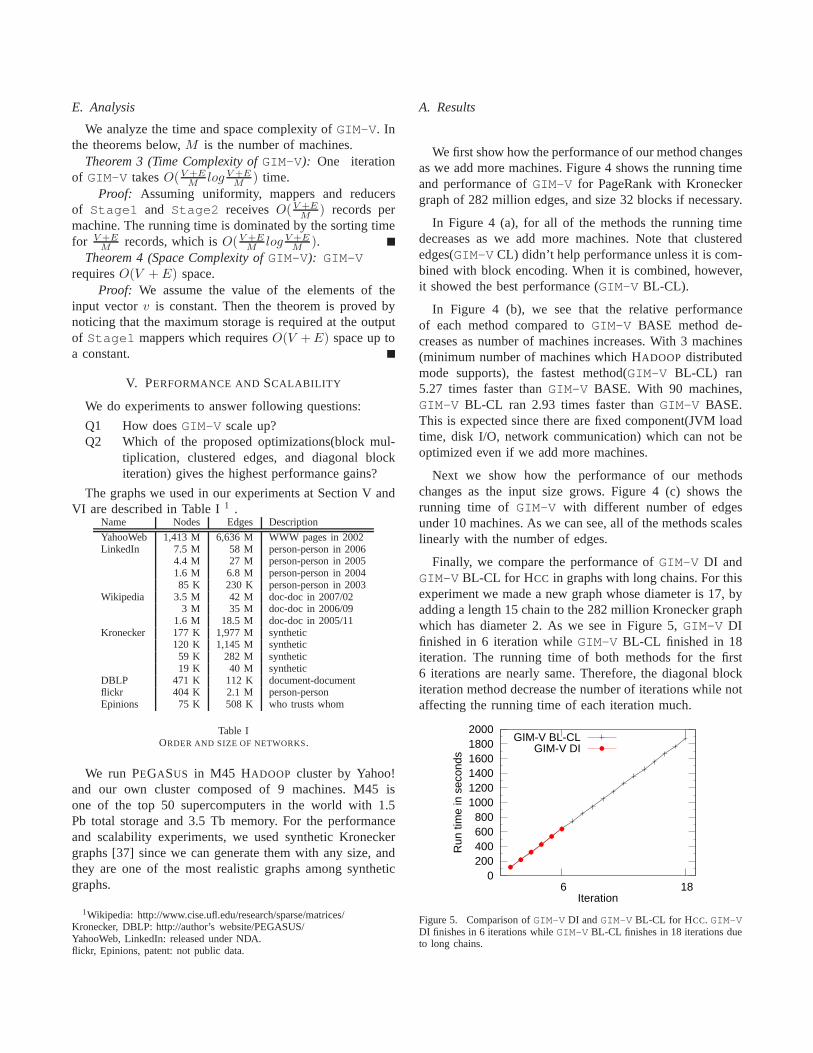
Finally, we compare the performance ofGIM-V DI andGIM-V BL-CL for HCC in graphs with long chains. For thisexperiment we made a new graph whose diameter is 17, byadding a length 15 chain to the 282 million Kronecker graphwhich has diameter 2. As we see in Figure 5,GIM-V DIfinished in 6 iteration whileGIM-V BL-CL finished in 18iteration. The running time of both methods for the first6 iterations are nearly same. Therefore, the diagonal blockiteration method decrease the number of iterations while notaffecting the running time of each iteration much.

0 200 400 600 800

1000 1200 1400 1600 1800 2000

6 18

Run

tim

e in

sec

onds

Iteration

GIM-V BL-CLGIM-V DI

Figure 5. Comparison ofGIM-V DI andGIM-V BL-CL for HCC. GIM-VDI finishes in 6 iterations whileGIM-V BL-CL finishes in 18 iterations dueto long chains.

0

200

400

600

800

1000

1200

1400

1600

0 10 20 30 40 50 60 70 80 90

Run

tim

e in

sec

onds

Number of machines

GIM-V BASEGIM-V CLGIM-V BL

GIM-V BL-CL

0

1

2

3

4

5

6

7

8

0 10 20 30 40 50 60 70 80 90

Per

form

ance

Number of machines

GIM-V BL-CLGIM-V BLGIM-V CL

GIM-V BASE

0

500

1000

1500

2000

2500

3000

3500

40M282M 1146M 1977M

Run

tim

e in

sec

onds

Number of edges

GIM-V BASEGIM-V CLGIM-V BL

GIM-V BL-CL

(a) Running time vs. Machines (b) Performance vs. Machines (c) Running time vs. EdgesFigure 4. Scalability and Performance of GIM-V. (a) Runningtime decreases quickly as more machines are added. (b) The performance(=1/runningtime) of ’BL-CL’ wins more than 5x (for n=3 machines) over the ’BASE’. (c) Every version ofGIM-V shows linear scalability.

VI. GIM-V AT WORK

In this section we use PEGASUS for mining very largegraphs. We analyze connected components, diameter, andPageRank of large real world graphs. We show that PE-GASUS can be useful for finding patterns, outliers, andinteresting observations.

A. Connected Components of Real Networks

We used the LinkedIn social network and Wikipedia page-linking-to-page network, along with the YahooWeb graph forconnected component analysis. Figure 6 show the evolutionof connected components of LinkedIn and Wikipedia data.Figure 7 show the distribution of connected components inthe YahooWeb graph. We have following observations.

Figure 7. Connected Components of YahooWeb. Notice the two anomalousspikes which are far from the constant-slope tail.

Power Law Tails in Connected Components Distri-butions We observed power law relation of count andsize of small connected components in Figure 6(a),(b) andFigure 7. This reflects that the connected components inreal networks are formed by processes similar to ChineseRestaurant Process and Yule distribution [38].

Stable Connected Components After Gelling PointIn Figure 6(a), the distribution of connected componentsremain stable after a ‘gelling’ point[39] at year 2003.We

can see that the slope of tail distribution do not change afteryear 2003. We observed the same phenomenon in Wikipediagraph in Figure 6 (b). The graph show stable tail slopes fromthe beginning, since the network were already mature in year2005.

Absorbed Connected Components and Dunbar’s num-ber In Figure 6(a), we find two large connected componentsin year 2003. However it became merged in year 2004.The giant connected component keeps growing, while thesecond and the third largest connected components do notgrow beyond size 100 until they are absorbed to the giantconnected component in Figure 6 (a) and (b). This agreeswith the observation[39] that the size of the second/thirdconnected components remains constant or oscillates. Lastly,the maximum connected component size except the giantconnected component in the LinkedIn graph agrees wellwith Dunbar’s number[40], which says that the maximumcommunity size in social networks is roughly 150.

Anomalous Connected ComponentsIn Figure 7, wefound two outstanding spikes. In the first spike at size300, more than half of the components have exactly thesame structure and they were made from a domain sellingcompany where each component represents a domain to besold. The spike happened because the companyreplicatedsites using the same template, and injected the disconnectedcomponents into WWW network. In the second spike atsize 1101, more than 80 % of the components are pornsites disconnected from the giant connected component. Bylooking at the distribution plot of connected components,we could find interesting communities with special purposeswhich are disconnected from the rest of the Internet.

B. PageRanks of Real Networks

We analyzed PageRank of YahooWeb graph with PEGA-SUS. Figure 8 shows the distribution of PageRank of thegraph. We observed that the PageRank follows a powerlaw distribution with exponent 1.97, which is very closeto the exponent 1.98 of the in-degree distribution of thesame graph. Pandurangan et. al.[41] observed that the twoexponent are same for 100,000 pages in Brown University

(a) Connected Components of LinkedIn (b) Connected Components of WikipediaFigure 6. The evolution of connected components. (a) The giant connected component grows for each year. However, the second largest connectedcomponent do not grow above Dunbar’s number(≈ 150) and the slope of the tail remains constant after the gelling point at year 2003. (b) As in LinkedIn,notice the growth of giant connected component and the constant slope for tails.

domain. Our result is that the same observation holds true for10,000 timeslarger network with 1.4billion pages snapshotof the Internet.

The top 3 highest PageRank sites at year 2002are www.careerbank.com, access.adobe.com, andtop100.rambler.ru. As expected, they have huge in-degrees (from≈70K to ≈70M).

Figure 8. PageRank distribution of YahooWeb. The distribution followspower law with exponent 1.97.

C. Diameter of Real Network

We analyzed the diameter and radius of real networks withPEGASUS. Figure 9 shows the radius plot of real networks.We have following observations:

Small Diameter For all the graphs in Figure 9, theaverage diameter was less than 6.09. This means that thereal world graphs are well connected.

Constant Diameter over Time For LinkedIn graph, theaverage diameter was in the range of 5.28 and 6.09. For

Wikipedia graph, the average diameter was in the range of4.76 and 4.99. Note that the diameter do not monotonicallyincrease as network grows: they remain constant or shrinksover time.

Bimodal Structure of Radius Plot For every plot,we observe bimodal shape which reflects the structure ofthese real graphs. The graphs have one giant connectedcomponent where majority of nodes belong to, and manysmaller connected components whose size follows powerlaw. Therefore, the first mode is at radius zero which comesfrom one-node components; second mode(e.g., at radius 6in Epinion) comes from the giant connected component.

100101102103104105106107108109

0 2 4 6 8 10 12 14 16 18

Num

ber

of N

odes

Radius

Avg Diameter: 5.89LinkedIn 2003

100101102103104105106107108109

0 2 4 6 8 10 12 14 16 18

Num

ber

of N

odes

Radius

Avg Diameter: 6.09LinkedIn 2004

100101102103104105106107108109

0 2 4 6 8 10 12 14 16 18

Num

ber

of N

odes

Radius

Avg Diameter: 5.28LinkedIn 2005

100101102103104105106107108109

0 2 4 6 8 10 12 14 16 18

Num

ber

of N

odes

Radius

Avg Diameter: 5.56LinkedIn 2006

100101102103104105106107108109

0 5 10 15 20 25 30 35

Num

ber

of N

odes

Radius

Avg Diameter: 4.99Wikipedia 2005

100101102103104105106107108109

0 5 10 15 20 25 30 35

Num

ber

of N

odes

Radius

Avg Diameter: 4.73Wikipedia 2006

100101102103104105106107108109

0 5 10 15 20 25 30 35

Num

ber

of N

odes

Radius

Avg Diameter: 4.76Wikipedia 2007

100101102103104105106107108109

0 2 4 6 8 10

Num

ber

of N

odes

Radius

Avg Diameter: 2.77DBLP doc-doc

100101102103104105106107108109

0 2 4 6 8 10 12 14 16 18

Num

ber

of N

odes

Radius

Avg Diameter: 3.72Flickr

100101102103104105106107108109

0 2 4 6 8 10 12 14 16 18

Num

ber

of N

odes

Radius

Avg Diameter: 3.82Epinion

Figure 9. Radius of real graphs.X axis: radius. Y axis: number of nodes.(Row 1) LinkedIn from 2003 to 2006.(Row 2) Wikipedia from 2005 to 2007.(Row 3) DBLP, flickr, Epinion.

VII. C ONCLUSIONS

In this paper we proposed PEGASUS, a graph miningpackage for very large graphs using the HADOOP architec-ture. The main contributions are followings:

• We identified the common, underlying primitive of sev-eral graph mining operations, and we showed that it is ageneralized form of a matrix-vector multiplication. Wecall this operation Generalized Iterative Matrix-Vectormultiplication and showed that it includes the diameterestimation, the PageRank estimation, RWR calculation,and finding connected-components, as special cases.

• Given its importance, we proposed several optimiza-tions (block-multiplication, diagonal block iteration etc)and reported the winning combination, which achieves5 timesfaster performance to the naive implementation.

• We implemented PEGASUS and ran it on M45, oneof the 50 largest supercomputers in the world (3.5 Tbmemory, 1.5Pb disk storage). Using PEGASUS and ouroptimized Generalized Iterative Matrix-Vector multipli-cation variants, we analyzed real world graphs to revealimportant patterns including power law tails, stabilityof connected components, and anomalous components.Our largest graph, “YahooWeb”, spanned 120Gb, andis one of the largest publicly available graph that wasever studied.

Other open source libraries such as HAMA (Hadoop Ma-trix Algebra) [42] can benefit significantly from PEGASUS.One major research direction is to add to PEGASUS aneigensolver, which will compute the topk eigenvectors andeigenvalues of a matrix. Another directions includes tensoranalysis on HADOOP ([43]), and inferences of graphicalmodels in large scale.

ACKNOWLEDGMENT

The authors would like to thank YAHOO! for providingus with the web graph and access to the M45.

This material is based upon work supported by the Na-tional Science Foundation under Grants No. IIS-0705359IIS0808661 and under the auspices of the U.S. Departmentof Energy by University of California Lawrence LivermoreNational Laboratory under contract DE-AC52-07NA27344(LLNL-CONF-404625), subcontracts B579447, B580840.

Any opinions, findings, and conclusions or recommenda-tions expressed in this material are those of the author(s) anddo not necessarily reflect the views of the National ScienceFoundation, or other funding parties.

REFERENCES

[1] A. Broder, R. Kumar, F. Maghoul, P. Raghavan, S. Ra-jagopalan, R. Stata, A. Tomkins, and J. Wiener, “Graphstructure in the web,”Computer Networks 33, 2000.

[2] J. Dean and S. Ghemawat, “Mapreduce: Simplified dataprocessing on large clusters,”OSDI, 2004.

[3] J. Chen, O. R. Zaiane, and R. Goebel, “Detectingcommunities in social networks using max-min modu-larity,” SDM, 2009.

[4] T. Falkowski, A. Barth, and M. Spiliopoulou, “Den-graph: A density-based community detection algo-rithm,” Web Intelligence, 2007.

[5] G. Karypis and V. Kumar, “Parallel multilevel k-way partitioning for irregular graphs,”SIAM Review,vol. 41, no. 2, 1999.

[6] S. Ranu and A. K. Singh, “Graphsig: A scalableapproach to mining significant subgraphs in large graphdatabases,”ICDE, 2009.

[7] Y. Ke, J. Cheng, and J. X. Yu, “Top-k correlative graphmining,” SDM, 2009.

[8] P. Hintsanen and H. Toivonen, “Finding reliable sub-graphs from large probabilistic graphs,”PKDD, 2008.

[9] J. Cheng, J. X. Yu, B. Ding, P. S. Yu, and H. Wang,“Fast graph pattern matching,”ICDE, 2008.

[10] F. Zhu, X. Yan, J. Han, and P. S. Yu, “gprune: A con-straint pushing framework for graph pattern mining,”PAKDD, 2007.

[11] C. Chen, X. Yan, F. Zhu, and J. Han, “gapprox:Mining frequent approximate patterns from a massivenetwork,” ICDM, 2007.

[12] X. Yan and J. Han, “gspan: Graph-based substructurepattern mining,”ICDM, 2002.

[13] N. S. Ketkar, L. B. Holder, and D. J. Cook, “Subdue:Compression-based frequent pattern discovery in graphdata,” OSDM, August 2005.

[14] M. Kuramochi and G. Karypis, “Finding frequentpatterns in a large sparse graph,”SIAM Data MiningConference, 2004.

[15] C. Wang, W. Wang, J. Pei, Y. Zhu, and B. Shi,“Scalable mining of large disk-based graph databases,”KDD, 2004.

[16] N. Wang, S. Parthasarathy, K.-L. Tan, and A. K. H.Tung, “Csv: Visualizing and mining cohesive sub-graph,”SIGMOD, 2008.

[17] S. Brin and L. Page, “The anatomy of a large-scalehypertextual (web) search engine.” inWWW, 1998.

[18] J. Kleinberg, “Authoritative sources in a hyperlinkedenvironment,” inProc. 9th ACM-SIAM SODA, 1998.

[19] C. E. Tsourakakis, U. Kang, G. L. Miller, andC. Faloutsos, “Doulion: Counting triangles in massivegraphs with a coin,”KDD, 2009.

[20] C. E. Tsourakakis, M. N. Kolountzakis, and G. L.Miller, “Approximate triangle counting,” Apr 2009.[Online]. Available: http://arxiv.org/abs/0904.3761

[21] U. Kang, C. Tsourakakis, A. Appel, C. Faloutsos,and J. Leskovec, “Hadi: Fast diameter estimation andmining in massive graphs with hadoop,”CMU-ML-08-117, 2008.

[22] T. Qian, J. Srivastava, Z. Peng, and P. C. Sheu, “Simul-taneouly finding fundamental articles and new topics

using a community tracking method,”PAKDD, 2009.[23] N. Shrivastava, A. Majumder, and R. Rastogi, “Mining

(social) network graphs to detect random link attacks,”ICDE, 2008.

[24] Y. Shiloach and U. Vishkin, “An o(logn) parallel con-nectivity algorithm,”Journal of Algorithms, pp. 57–67,1982.

[25] B. Awerbuch and Y. Shiloach, “New connectivity andmsf algorithms for ultracomputer and pram,”ICPP,1983.

[26] D. Hirschberg, A. Chandra, and D. Sarwate, “Com-puting connected components on parallel computers,”Communications of the ACM, vol. 22, no. 8, pp. 461–464, 1979.

[27] J. Greiner, “A comparison of parallel algorithms forconnected components,”Proceedings of the 6th ACMSymposium on Parallel Algorithms and Architectures,June 1994.

[28] G. Aggarwal, M. Data, S. Rajagopalan, and M. Ruhl,“On the streaming model augmented with a sortingprimitive,” Proceedings of FOCS, 2004.

[29] R. Lammel, “Google’s mapreduce programming model– revisited,” Science of Computer Programming,vol. 70, pp. 1–30, 2008.

[30] “Hadoop information,” http://hadoop.apache.org/.[31] C. Olston, B. Reed, U. Srivastava, R. Kumar, and

A. Tomkins, “Pig latin: a not-so-foreign language fordata processing,” inSIGMOD ’08, 2008, pp. 1099–1110.

[32] S. Papadimitriou and J. Sun, “Disco: Distributed co-clustering with map-reduce,”ICDM, 2008.

[33] R. Chaiken, B. Jenkins, P.-A. Larson, B. Ramsey,D. Shakib, S. Weaver, and J. Zhou, “Scope: easyand efficient parallel processing of massive data sets,”VLDB, 2008.

[34] R. Pike, S. Dorward, R. Griesemer, and S. Quinlan,“Interpreting the data: Parallel analysis with sawzall,”Scientific Programming Journal, 2005.

[35] R. L. Grossman and Y. Gu, “Data mining using highperformance data clouds: experimental studies usingsector and sphere,”KDD, 2008.

[36] J.-Y. Pan, H.-J. Yang, C. Faloutsos, and P. Duygulu,“Automatic multimedia cross-modal correlation discov-ery,” ACM SIGKDD, Aug. 2004.

[37] J. Leskovec, D. Chakrabarti, J. M. Kleinberg, andC. Faloutsos, “Realistic, mathematically tractable graphgeneration and evolution, using kronecker multiplica-tion,” PKDD, 2005.

[38] M. E. J. Newman, “Power laws, pareto distributionsand zipf’s law,” Contemporary Physics, no. 46, pp.323–351, 2005.

[39] M. Mcglohon, L. Akoglu, and C. Faloutsos, “Weightedgraphs and disconnected components: patterns and agenerator,”KDD, pp. 524–532, 2008.

[40] R. Dunbar, “Grooming, gossip, and the evolution oflanguage,”Harvard Univ Press, October 1998.

[41] G. Pandurangan, P. Raghavan, and E. Upfal, “Usingpagerank to characterize web structure,”COCOON,August 2002.

[42] “Hama website,” http://incubator.apache.org/hama/.[43] T. G. Kolda and J. Sun, “Scalable tensor decompsitions

for multi-aspect data mining,”ICDM, 2008.