Embed Size (px)
Citation preview
Quantitative Mechanical Property Mapping at the Nanoscale with
PeakForce QNM
INTRODUCTION
The scanning probe microscope
(SPM)1 has long been recognized as a
useful tool for measuring mechanical
properties of materials. Until recently
though, it has been impossible to
achieve truly quantitative material
property mapping with the resolution
and convenience demanded by SPM
researchers. A number of recent SPM
mode innovations have taken aim at
these limitations, and now, with the
release of PeakForce QNM™ by Veeco, it
is possible to identify material variations
unambiguously and at high resolution
across a topographic image. This
application note discusses the principles
and benefits of the PeakForce QNM
imaging mode.
SPM AND MECHANICAL
PROPERTY MAPPING
Researchers often use the SPM to
acquire the force on the tip versus
its vertical position. The resulting
“force curves” can then be analyzed to
determine a host of characteristics of
the material beneath the tip. However,
these force curves can only provide
data at one point on the sample surface
at a time. The technique of force
volume imaging collects force curves
at each pixel in an image and puts
them together to map the properties
across a larger sample.2 Though more
information is gathered, force volume
imaging is typically very slow, which
makes detailed mapping impractical.
To solve this problem, Pulsed Force
Mode was developed. This approach
improves speed by using a relatively
fast sinusoidal ramping.3 Unfortunately,
this also makes the material property
measurements less quantitative.
Veeco’s development of TappingMode™
imaging in 19934 was a key step
forward in the functionality of SPM.4 In
TappingMode the probe is vibrated near
the resonant frequency of the cantilever
while it is scanned across the sample.
The tip only contacts the surface for a
small percentage of the time, keeping
the tapping force low and the lateral
forces negligible. Consequently,
TappingMode has the ability to generate
high-quality data for a wide range
of samples, making it the dominant
imaging mode for most SPM applications
over the last ten years.
The data types obtained from
TappingMode SPM are primarily
topography and phase. PhaseImagingTM
creates images of the phase of
the tapping response, which is a function
of the forces that the tip is experiencing.
Since the probe is oscillating, it
experiences attractive and repulsive
forces depending on its position in
the cycle in a way that is analogous
to force curves. A drawback to the
technique is that the resonant behavior
of the probe also acts as a filter,
making it impractical to reconstruct the
force curves with sufficient precision
to extract quantitative mechanical
information.5–6 In 2008, Veeco released
HarmoniX® as a solution to this
problem. HarmoniX adds a second
sensor with a much higher bandwidth
by offsetting the tip and measuring the
torsional signal.7–9 This technique has
been successful in resolving material
components in complex polymeric
systems. The downsides of this approach
are that (1) it requires special probes,
(2) the operation of the technique can
be complicated (especially in fluid),
and (3) interpretation of the results is
sometimes difficult.
PeakForce QNM is a new mode
developed by Veeco that provides
By: Bede Pittenger, Natalia Erina, Chanmin Su Veeco Instruments Inc.
PAGE 2 Quantitative Mechanical Property Mapping at the Nanoscale with PeakForce QNM
the capabilities of HarmoniX without
the complexity of operation and
interpretation. Additionally, no special
probes are required (although careful
choice of probes is essential for best
performance). PeakForce QNM uses
Veeco’s new Peak Force Tapping™
technology for system feedback to
deliver a number of important benefits:
• High-resolution mapping of
mechanical properties – Scanning
speeds and number of pixels in an
image are similar to TappingMode.
Analysis of force curve data is
done on the fly, providing a map
of multiple mechanical properties
that has the same resolution
as the height image. Sample
deformation depths are limited to a
few nanometers, minimizing
the loss of resolution that can occur
with larger tip-sample contact areas.
• Non-destructive to tips and samples
– Peak Force Tapping provides direct
control of the maximum normal
force (and thus the deformation
depth) of the sample, while
eliminating lateral forces. This
preserves both the tip and sample.
Additionally, Peak Force Tapping
enables Veeco’s new ScanAsyst™
feature, which automatically adjusts
the scanning parameters in real-
time to optimize the image and
protect the probe and sample.
• Unambiguous and quantitative data
over a wide range of materials –
Analysis of the entire force curve for
each tap allows different properties
to be independently measured.
Since a wide selection of probes
is available, it is possible to cover
a very broad range of modulus
or adhesion parameters while
maintaining excellent signal-to-
noise ratios.
PEAK FORCE TAPPING
In scanning probe microscopy, there
are two primary causes of tip and
sample damage. Any lateral force that
the tip exerts on the sample can cause
the sample to tear (the tip plows through
the sample). Likewise, lateral forces
from a hard sample can cause the end of
the tip to fracture and break off. Normal
forces can also cause damage to both tip
and sample. Even if there is not enough
normal force to damage the sample,
there can still be enough to deform
the sample, increasing the contact area
(and the effective probe size) and
reducing the resolution of the scan.
In Peak Force Tapping, the probe and
sample are intermittently brought
together (similar to TappingMode) to
contact the surface for a short period,
which eliminates lateral forces. Unlike
TappingMode where the feedback loop
keeps the cantilever vibration amplitude
constant, Peak Force Tapping controls
the maximum force (Peak Force) on
the tip. This protects the tip and sample
from damage while allowing the tip-
sample contact area to be minimized.
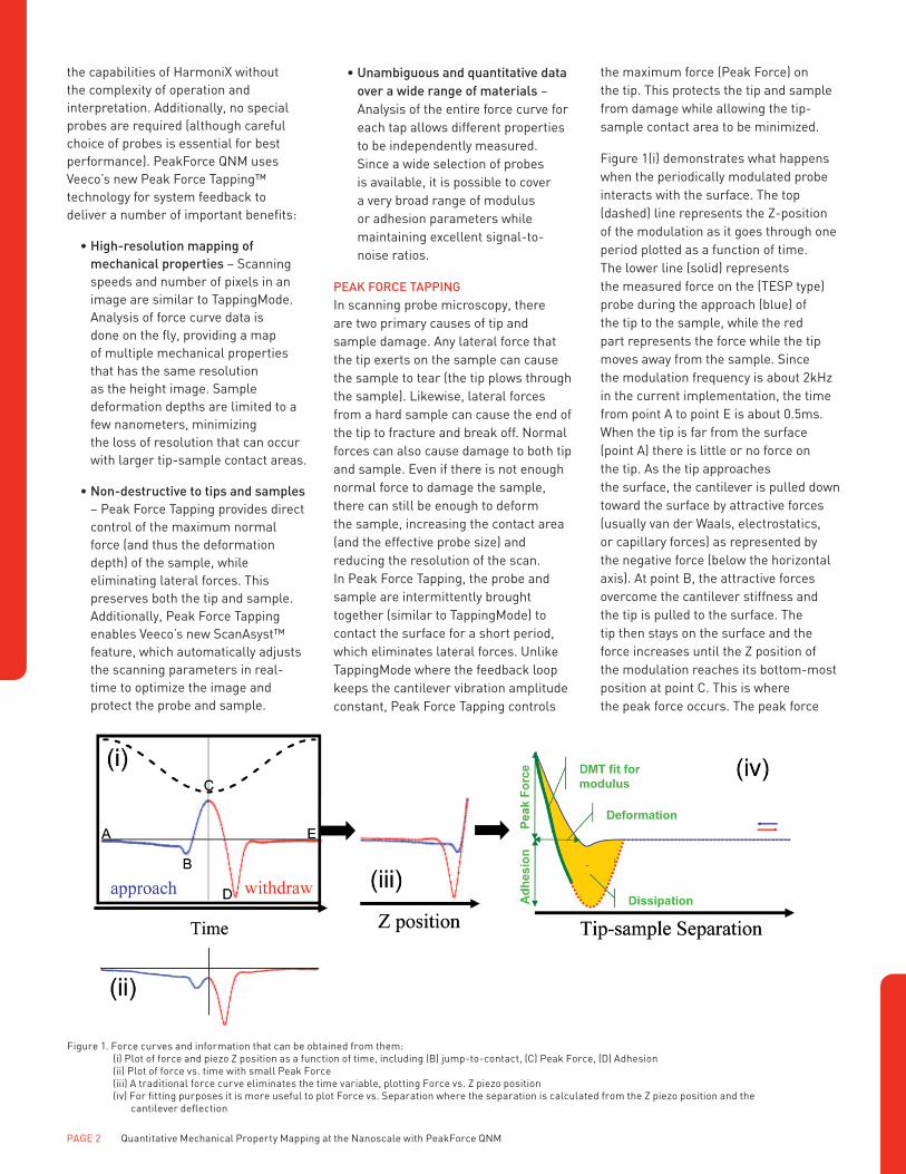
Figure 1(i) demonstrates what happens
when the periodically modulated probe
interacts with the surface. The top
(dashed) line represents the Z-position
of the modulation as it goes through one
period plotted as a function of time.
The lower line (solid) represents
the measured force on the (TESP type)
probe during the approach (blue) of
the tip to the sample, while the red
part represents the force while the tip
moves away from the sample. Since
the modulation frequency is about 2kHz
in the current implementation, the time
from point A to point E is about 0.5ms.
When the tip is far from the surface
(point A) there is little or no force on
the tip. As the tip approaches
the surface, the cantilever is pulled down
toward the surface by attractive forces
(usually van der Waals, electrostatics,
or capillary forces) as represented by
the negative force (below the horizontal
axis). At point B, the attractive forces
overcome the cantilever stiffness and
the tip is pulled to the surface. The
tip then stays on the surface and the
force increases until the Z position of
the modulation reaches its bottom-most
position at point C. This is where
the peak force occurs. The peak force
Figure 1. Force curves and information that can be obtained from them:
(i) Plot of force and piezo Z position as a function of time, including (B) jump-to-contact, (C) Peak Force, (D) Adhesion
(ii) Plot of force vs. time with small Peak Force
(iii) A traditional force curve eliminates the time variable, plotting Force vs. Z piezo position
(iv) For fitting purposes it is more useful to plot Force vs. Separation where the separation is calculated from the Z piezo position and the
cantilever deflection
Quantitative Mechanical Property Mapping at the Nanoscale with PeakForce QNM PAGE 3
(force at point C) during the interaction
period is kept constant by the system
feedback. The probe then starts to
withdraw and the force decreases
until it reaches a minimum at point D.
The adhesion is given by the force at this
point. The point where the tip comes off
the surface is called the pull-off point.
This often coincides with the minimum
force. Once the tip has come off
the surface, only long range forces affect
the tip, so the force is very small or zero
when the tip-sample separation is at its
maximum (point E).
As the system scans the tip across
the sample, the feedback loop of
the system maintains the instantaneous
force at point C at a constant value by
adjusting the extension of the Z piezo.
Figure 1(ii) illustrates an interesting
and unique challenge for peak force
control. Here the controlled peak force
at point C is actually attractive. This
can occur when the peak force is small
and the attractive forces are relatively
large. Looking at the measured force
in this plot, one might infer that the
force at C is not the maximum force.
In fact, the addition of the long range
attractive forces cause the stress
beneath the center of the probe tip to
be compressive (and greater) at point C
even though the measured force on
the probe is less than that at point A.
The small peak in the attractive
background is caused by the repulsive
force at the very apex point of the tip.
The total interaction force is integrated
over all of the tip atoms. While the tip
apex atoms feel a repulsive force, the
neighbor atoms, which consist of far
more volume, can still be feeling an
attractive force. This leads to a net
negative force overall. Even when
the peak force is negative, Peak
Force Tapping can recognize the local
maximum and maintain control of
the imaging process.
Figure 1(iii) shows the same data as
figure1(i) but with the force plotted as a
function of the distance. Since we control
the Z position of the modulation as a
function of time and we measure the
deflection of the cantilever as a function
of time, it is possible to eliminate the
time variable and plot the force against
the Z-position. These plots can then
be compared directly with the force-
distance curves that have been used
for decades by researchers interested
in measuring mechanical properties
of their samples with SPM, but at a
several orders of magnitude faster
measurement speed. One complication
of the fast data acquisition is the
excitation of cantilever resonance at the
pull-off point. This ringing is negligible
for a stiff lever, such as the TESP used
in figure 1. The oscillation is more
pronounced for softer levers. Peak
Force Tapping control has the ability to
identify the repulsive force and respond
to this interaction only, regardless of
the magnitude of the snap-off ringing.
Once a force curve is obtained, it is must
be converted to a force versus separation
plot for fitting and further analysis.
The tip-sample separation is different
from the Z position of the modulation
since the cantilever bends. Figure 1(iv)
is a sample of a force-separation plot
illustrating the types of information that
can be obtained. The most commonly
used quantities are elastic modulus,
tip-sample adhesion, energy dissipation,
and maximum deformation.
QUANTITATIVE MATERIAL PROPERTY
MAPPING
The foundation of material property
mapping with PeakForce QNM is
the ability of the system to acquire and
analyze the individual force curves from
each tap that occurs during the imaging
process. To separate the contributions
from different material properties such
as adhesion, modulus, dissipation,
and deformation, it is necessary to
measure the instantaneous force on
the tip rather than a time-average of
the force or dissipation over time, as is
done in TappingMode PhaseImaging™.
This requires a force sensor that has a
significantly higher bandwidth than the
frequency of the periodic interactions. In
Peak Force Tapping, the modulation
frequency is intentionally chosen to be
significantly lower than the cantilever
resonant frequency. The force
measurement bandwidth of a cantilever
is approximately equal to the resonant
frequency of the fundamental bending
mode used for force detection. As a
result, a properly chosen cantilever
is able to respond to changes in
instantaneous interaction force with an
immediate deflection change during
Peak Force Tapping.
As mentioned above, the force curve is
converted to a force versus separation
plot (see figure 1(iv)) for fitting and
further analysis. The separation, which
is the negative of the deformation
(sometimes called indentation
depth), is obtained by adding the Z
position of the piezo modulation to
the cantilever deflection. A constant
can be added to the separation to
make it zero at the point of contact
if it can be determined, but this is
not required for many analyses. This
process is equivalent to removing
frame compliance in indentation
measurements. These force-separation
curves are analogous to the load-
indentation curves commonly used
in nanoindentation.
The curves are then analyzed to obtain
the properties of the sample (adhesion,
modulus, deformation, and dissipation)
and the information is sent to one of
the image data channels while imaging
continues at usual imaging speeds.
The result is images that contain maps
of material properties (false colored
with a user selectable color table).
Since the system can acquire up to eight
channels at once, it is possible to map
all of the currently calculated properties
in a single pass. Offline analysis
functions can calculate statistics of
the mechanical properties of different
regions and sections through the data to
show the spatial distribution of
the properties.
Figure 1(iv) illustrates how common
mechanical properties are extracted
from calibrated force-separation
curves. Analysis of the force curves with
other models is possible by capturing
raw data with the “High-Speed Data
Capture” function. High-speed data
capture provides about 64,000 raw force
curves (typically several scan lines)
that can be captured at any time during
scanning and can later be correlated
with the analyzed data in the image. This
allows users to apply their own models
to the raw data to study more unusual
materials and properties.
PAGE 4 Quantitative Mechanical Property Mapping at the Nanoscale with PeakForce QNM
Elastic Modulus
To obtain the Young’s Modulus,
the retract curve is fit (see the bold
green line in figure 1(iv)) using
the Derjaguin–Muller–Toporov (DMT)
model10
F – Fadh is the force on the cantilever
relative to the adhesion force, R is the tip
end radius, and d – d0 is the deformation
of the sample. The result of the fit is
the reduced modulus E*. If the Poisson’s
ratio is known, the software can use
that information to calculate the Young’s
Modulus of the sample (Es). This is
related to the sample modulus by
the equation
We assume that the tip modulus Etip
is infinite, and calculate the sample
modulus using the sample Poisson’s
Ratio (which must be entered by the user
into the NanoScope® “Cantilever
Parameters”). The Poisson’s ratio
generally ranges between about 0.2 and
0.5 (perfectly incompressible) giving a
difference between the reduced
modulus and the sample modulus
between 4% and 25%. Since
the Poisson’s ratio is not generally
accurately known, many publications
report only the reduced modulus.
Entering zero for the parameter will
cause the system to return
the reduced modulus.
PeakForce QNM provides quantitative
modulus results over the range
of 700kPa to 70GPa provided
the appropriate probe is selected and
calibrated, and provided that the DMT
model is applicable. Calibration is done
either by comparing to a reference
sample (relative method), or by
measurement of tip end radius and
spring constant (absolute method).
In either method, the deflection
sensitivity must also be measured. While
calibration is still a several step process,
it has been made significantly easier
than HarmoniX calibration by eliminating
several steps and by automating
the calculation of several parameters.
An experienced user can complete a
calibration in less than ten minutes.
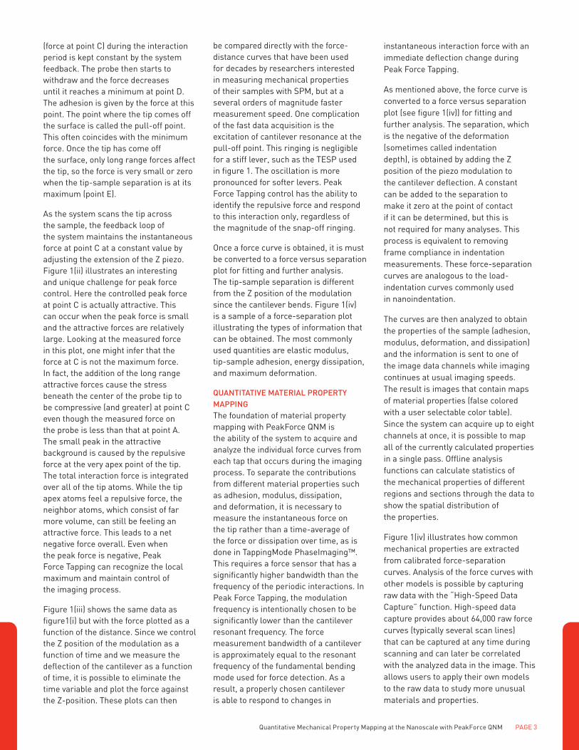
Figure 2 demonstrates that this works
for a wide range of materials from
polydimethylsiloxanes to silica. The
data in figure 2 was collected with a
set of probes that were selected to
have the most accuracy over a range of
modulus. Figure 3 lists the probe types
used and gives the approximate modulus
range for each probe type. The data was
acquired on homogeneous samples and
the system was calibrated using
the absolute method.
If the DMT model is not appropriate,
the modulus map will still return the fit
result, but it will be only qualitative.
Some cases where the DMT model
are not appropriate include cases
where the tip-sample geometry is not
approximated by a hard sphere (the
tip) contacting an elastic plane, cases
where mechanisms of deformation
other than elastic deformation are
active during the retracting part of
the curve (at these time scales), and
cases where the sample is confined
vertically or laterally by surrounding
material (close enough to effect the
strain in the deformed region). If this
is suspected, High Speed Data Capture
Figure 2. Plot of Measured Modulus vs. expected Young’s Modulus (from the literature or from SPM
Nanoindentation). Multiple probes were used with different spring constants to cover the entire range.
Each probe was individually calibrated using the absolute method.
Figure 3. Modulus ranges covered by various probes. The modulus and Veeco part number of the reference
sample for each range is also indicated.
F – Fadh = 4 E* .R(d – d0)3
3
E* = +1 – νs
2
Es
1 – νtip2
–1
Etip .
Quantitative Mechanical Property Mapping at the Nanoscale with PeakForce QNM PAGE 5
can acquire the individual force curves
across a section of interest to examine
the force curves directly and potentially
apply more advanced fitting models.
PeakForce QNM can be quite repeatable
if care is taken in the calibration process.
Recent experiments on homogeneous
samples where the absolute method
was used to measure samples in a range
between 1MPa and 400MPa ten times
each (with different probes) resulted
in a relative standard deviation of less
than 25% for all samples. If the goal is
to discriminate between components
in a multi-component system where
the modulus of one component is
known, the modulus noise level is more
interesting. For the measurements in
the study, the relative standard deviation
was never more than 6%.
Adhesion
The second mechanical property
acquired in the mapping is the adhesion
force, illustrated by the minimum
force in figure 1(iv). The source of
the adhesion force can be any attractive
force between the tip and sample. In
air, van der Waals, electrostatics, and
forces due to the formation of a capillary
meniscus can all contribute with the
relative strengths of the contributions
depending on such parameters as
Hamaker constants, surface charges,
and hydrophilicity. For example, if
either sample or the probe surface
is hydrophilic, a capillary meniscus
will typically form, leading to higher
adhesion that extends nanometers
beyond the surface. For polymers in
which the long molecules serve as a
meniscus, the adhesion can extend
tens of nanometers beyond the surface.
The adhesion typically increases with
increasing probe end radius. Simple
models based on surface energy
arguments predict the adhesion to be
proportional to the tip end radius.11
The area below the zero force reference
(the horizontal line in the force curve)
and above the withdrawing curve is
referred to as “the work of adhesion.”
The energy dissipation is dominated by
work of adhesion if the peak force set
point is chosen such that the non-elastic
deformation area (the hysteresis above
the zero force reference) in the loading-
unloading curve is negligible compared
to the work of adhesion.
Adhesion force becomes a much more
meaningful and important quantity if
the tip is functionalized. In this case,
the adhesion reflects the chemical
interaction between specific molecules
on the tip and sample. The adhesion map
in this case carries the
chemical information.
Dissipation
Energy dissipation is given by the force
times the velocity integrated over one
period of the vibration (represented by
the gold area in the figure 1(iv)):
where W represents energy dissipated
in a cycle of interaction. F is
the interaction force vector and dZ is
the displacement vector. Because the
velocity reverses its direction in each
half cycle, the integration is zero if the
loading and unloading curves coincide.
For pure elastic deformation there is
no hysteresis betweenthe repulsive
parts of the loading-unloading curve,
corresponding to very low dissipation.
In this case the work of adhesion
becomes the dominant contributor to
energy dissipation. Energy dissipated
is presented in electron volts as
the mechanical energy lost per
tapping cycle.
Deformation
The fourth property is the maximum
deformation, defined as the penetration
of the tip into the surface at the peak
force, after subtracting cantilever
compliance. As the load on the sample
under the tip increases, the deformation
also increases, reaching a maximum
at the peak force. The measured
deformation may include both elastic
and plastic contributions. With known tip
shape and contact area, this parameter
can also be converted to the hardness
(although this is usually only applied in
cases where the dominant deformation
mechanism is plastic deformation).
Maximum sample deformation is
calculated from the difference in
separation from the point where
the force is zero to the peak force point
along the approach curve (see figure
1(iv)). There may be some error in this
measurement due to the fact that the tip
first contacts the surface at the jump-to-
contact point (figure 1(i), point B) rather
than at the zero crossing.
COMPARISON WITH FORCE VOLUME AND
PULSED FORCE MODE
The earliest mechanical property
mapping was performed by force
volume, which is still often used to
acquire quantitative nanomechanical
data. Force volume collects force
curves triggered by the same maximum
repulsive force while scanning back and
forth over the surface. Collecting a force
volume image usually takes several
hours because individual force curves
generally take about a second to collect,
and a map needs thousands of force
curves to be useful. This speed limitation
was greatly improved by Pulsed Force
Mode, which modulates the Z piezo at
about 1 kHz, allowing property mapping
in much shorter time. Pulsed Force
Mode is primarily used as a property
mapping method with the trigger force
of a few nanonewtons or more. Below
one nanonewton, parasitic motion of
the cantilever can dominate and cause
feedback instability.
Peak Force Tapping modulates the Z
piezo in a similar fashion to force volume
and Pulsed Force Mode. However, it can
operate with interaction forces orders of
magnitude lower, i.e., piconewtons. Such
high-precision force control is enabled
by data pattern analysis within each
interaction period. When the relative Z
position between the probe and sample
is modulated, various parasitic cantilever
motions can occur (defined as variation
in the cantilever deflection that occurs
when the tip is not interacting with
the sample). These motions include
cantilever oscillation excited by the pull-
off, as well as deflections triggered by
harmonics of the piezo motion or viscous
forces in air or fluid. The parasitic
deflection limits the ability of Pulsed
Force Mode to operate with very low
forces. Low force control happens to be
the most important factor in achieving
high-resolution imaging and property
measurements. For example, if the tip
W = T
0
F dZ = F νdt ,

PAGE 6 Quantitative Mechanical Property Mapping at the Nanoscale with PeakForce QNM
Figure 4. Multilayer polymer optical film comparing results obtained with Tapping Mode Phase Imaging (a-c) and PeakForce QNM (d-f) (10μm scan size).
The phase image in (b) was collected with an amplitude setpoint of 80% of the free amplitude, while the amplitude setpoint in (c) was 40%. The trace profile from
(f) is the modulus along the line in (f) from left to right. Note that the tapping phase result (b) is nearly identical to the PeakForce QNM adhesion image (e) and
the contrast is inverted relative to the modulus image.
end has 1 nm2 area, 1nN force will lead
to 1GPa stress at the tip end. Such
stress is sufficient to break a silicon tip.
To lower the stress below the fracture
stress of silicon, the control force needs
to be no more than a few hundred
piconewtons. For samples softer than
silicon, the required controlling force to
avoid significant deformation or damage
is even lower.
During Peak Force Tapping operation,
the parasitic deflection signal and its
data pattern are analyzed by comparing
the known sources of force artifacts,
such as cantilever resonance at pull-off,
harmonics of the modulations, and other
system actuation sources. The signature
of the interaction is extracted from
the parasitic deflections. The feedback
loop can choose any point in the force
curve to control tip-sample interactions
instantaneously. For Peak Force
Tapping, the peak point in the repulsive
interaction is chosen as the control
parameter, similar to the triggered level
in force volume mapping.
A major advantage of Peak Force
Tapping is its broad operating force
range, from piconewtons to
micronewtons. At the high-force end, it
coincides with traditional mechanical
mapping techniques, namely force
volume and Pulsed Force Mode, yet can
generate quantitative data with the new
advanced quantitative nanomechanical
procedure. In the low-force regime, it
matches the interaction force achievable
by light tapping in TappingMode but with
much improved stability and ease of use
in all environments.
COMPARISON WITH TAPPINGMODE
AND HARMONIX
The phase of the TappingMode
cantilever vibration relative to the drive
is a useful indication of different
mechanical properties. Unfortunately,
the phase signal reflects a mixture of
material properties, depending both on
dissipative and conservative forces.12–13
Since elasticity, hardness, adhesion
and energy dissipation all contribute
to phase shift, phase alone does not
provide enough information to quantify
or discriminate between all of these
properties. Additionally, the phase signal
depends on imaging parameters such
as drive amplitude, drive frequency,
Quantitative Mechanical Property Mapping at the Nanoscale with PeakForce QNM PAGE 7
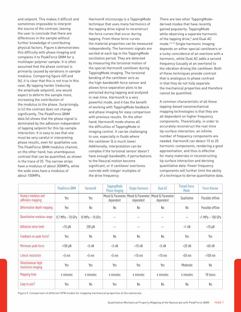
Figure 5. Comparison of different SPM modes for mapping mechanical properties at the nanoscale.
PeakForce QNM
Young’s modulus andadhesion mapping
Deformation depth mapping
Yes
Yes
0.7 MPa – 70 GPa
<10 pN
Yes
<100 pN
<5 nm
Yes
4 minutes
Yes
Mixed & Parameterdependent
No
—
—
No
<3 nN
<5 nm
Yes
4 minutes
Yes
Mixed & Parameterdependent
No
—
—
No
<10 nN
<10 nm
Yes
4 minutes
No
Mixed & Parameterdependent
No
—
—
No
<5 nN
<10 nm
Yes
4 minutes
No
Yes
No
10 MPa – 10 GPa
200 pN
No
<5 nN
<5 nm
Yes
4 minutes
No
Qualitative
No
—
<1 nN
Yes
<20 nN
<50 nm
Moderate
4 minutes
No
Possible offline
Possible offline
<1 MPa – 100 GPa
<10 pN
Yes
<50 nN
<100 nm
No
18 hours
No
Quantitative modulus range
Adhesion noise level
Feedback on peak force?
Minimum peak force
Lateral resolution
Mapping time
Easy to use?
Simultaneous high resolution imaging
HarmoniX Single Harmonic Dual AC Force VolumeTappingMode
Phase ImagingPulsed Force
Mode
and setpoint. This makes it difficult and
sometimes impossible to interpret
the source of the contrast, leaving
the user to conclude that there are
differences in the sample without
further knowledge of contributing
physical factors. Figure 4 demonstrates
this difficulty with phase imaging and
compares it to PeakForce QNM for a
multilayer polymer sample. It is often
assumed that the phase contrast is
primarily caused by variations in sample
modulus. Comparing figure 4(f) and
(b), it is clear that this is not true in this
case. By tapping harder (reducing
the amplitude setpoint), one would
expect to deform the sample more,
increasing the contribution of
the modulus to the phase. Surprisingly,
in (c) the contrast does not change
significantly. The PeakForce QNM
data (e) shows that the phase signal is
dominated by the adhesion independent
of tapping setpoint for this tip-sample
interaction. It is easy to see that one
must be very careful in interpreting
phase results, even for qualitative use.
The PeakForce QNM modulus channel,
on the other hand, has unambiguous
contrast that can be quantified, as shown
in the trace of (f). The narrow strips
have a modulus of about 300MPa, while
the wide ones have a modulus of
about 100MPa.
HarmoniX microscopy is a TappingMode
technique that uses many harmonics of
the tapping drive signal to reconstruct
the force curves that occur during
tapping. From these force curves
the material properties can be measured
independently. The harmonic signals are
excited at each tap in the TappingMode
oscillation period. They are detected
by measuring the torsional motion of
the special HarmoniX cantilever during
TappingMode imaging. The torsional
bending of the cantilever acts as
the high-bandwidth force sensor and
allows force separation plots to be
extracted during tapping and analyzed
in real-time. HarmoniX is a very
powerful mode, and it has the benefit
of working with TappingMode feedback
and phase imaging for easy comparison
with previous results. On the other
hand, HarmoniX mode shares all
the difficulties of TappingMode in
imaging control. It can be challenging
to use, especially in fluids where
the cantilever Q is much lower.
Additionally, interpretation can be
complex if the torsional sensor doesn’t
have enough bandwidth, if perturbations
to the flexural motion become
significant, or if cantilever overtones
coincide with integer multiples of
the drive frequency.
There are two other TappingMode-
derived modes that have recently
gained popularity: TappingMode
while observing a separate harmonic
of the tapping drive,5 and Dual AC
mode.14–15 Single harmonic imaging
depends on either special cantilevers or
a lucky coincidence of an overtone with a
harmonic, while Dual AC adds a second
frequency (usually at an overtone) to
the vibration driving the cantilever. Both
of these techniques provide contrast
that is analogous to phase contrast
in that they do not fully separate
the mechanical properties and therefore
cannot be quantified.
A common characteristic of all these
tapping-based nanomechanical
mapping technologies is that they are
all dependent on higher frequency
components. Theoretically, in order to
accurately reconstruct the real-time
tip-surface interaction, an infinite
number of frequency components are
needed. HarmoniX can detect 15 to 20
harmonic components, rendering a good
approximation, and thus is effective
for many materials in reconstructing
tip surface interaction and deriving
quantitative data. Fewer frequency
components will further limit the ability
of a technique to derive quantitative data.
PAGE 8 Quantitative Mechanical Property Mapping at the Nanoscale with PeakForce QNM
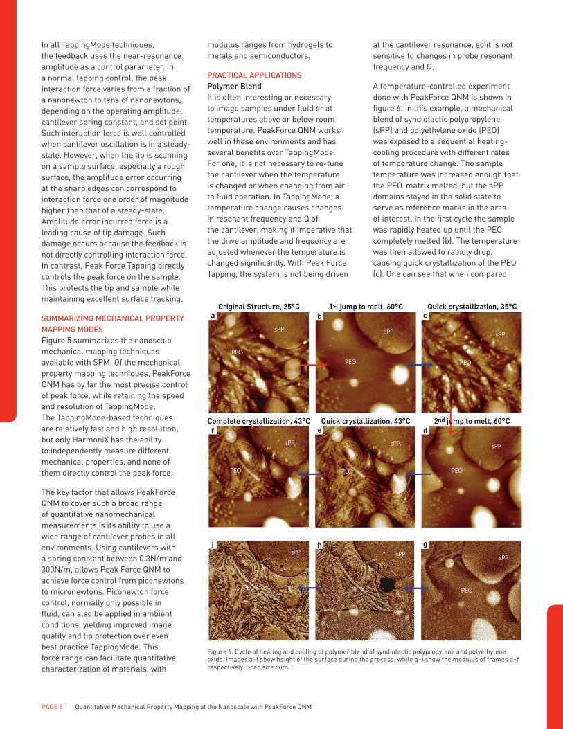
Figure 6. Cycle of heating and cooling of polymer blend of syndiotactic polypropylene and polyethylene
oxide. Images a–f show height of the surface during the process, while g–i show the modulus of frames d–f
respectively. Scan size 5um.
In all TappingMode techniques,
the feedback uses the near-resonance
amplitude as a control parameter. In
a normal tapping control, the peak
interaction force varies from a fraction of
a nanonewton to tens of nanonewtons,
depending on the operating amplitude,
cantilever spring constant, and set point.
Such interaction force is well controlled
when cantilever oscillation is in a steady-
state. However, when the tip is scanning
on a sample surface, especially a rough
surface, the amplitude error occurring
at the sharp edges can correspond to
interaction force one order of magnitude
higher than that of a steady-state.
Amplitude error incurred force is a
leading cause of tip damage. Such
damage occurs because the feedback is
not directly controlling interaction force.
In contrast, Peak Force Tapping directly
controls the peak force on the sample.
This protects the tip and sample while
maintaining excellent surface tracking.
SUMMARIZING MECHANICAL PROPERTY
MAPPING MODES
Figure 5 summarizes the nanoscale
mechanical mapping techniques
available with SPM. Of the mechanical
property mapping techniques, PeakForce
QNM has by far the most precise control
of peak force, while retaining the speed
and resolution of TappingMode.
The TappingMode-based techniques
are relatively fast and high resolution,
but only HarmoniX has the ability
to independently measure different
mechanical properties, and none of
them directly control the peak force.
The key factor that allows PeakForce
QNM to cover such a broad range
of quantitative nanomechanical
measurements is its ability to use a
wide range of cantilever probes in all
environments. Using cantilevers with
a spring constant between 0.3N/m and
300N/m, allows Peak Force QNM to
achieve force control from piconewtons
to micronewtons. Piconewton force
control, normally only possible in
fluid, can also be applied in ambient
conditions, yielding improved image
quality and tip protection over even
best practice TappingMode. This
force range can facilitate quantitative
characterization of materials, with
modulus ranges from hydrogels to
metals and semiconductors.
PRACTICAL APPLICATIONS
Polymer Blend
It is often interesting or necessary
to image samples under fluid or at
temperatures above or below room
temperature. PeakForce QNM works
well in these environments and has
several benefits over TappingMode.
For one, it is not necessary to re-tune
the cantilever when the temperature
is changed or when changing from air
to fluid operation. In TappingMode, a
temperature change causes changes
in resonant frequency and Q of
the cantilever, making it imperative that
the drive amplitude and frequency are
adjusted whenever the temperature is
changed significantly. With Peak Force
Tapping, the system is not being driven
at the cantilever resonance, so it is not
sensitive to changes in probe resonant
frequency and Q.
A temperature-controlled experiment
done with PeakForce QNM is shown in
figure 6. In this example, a mechanical
blend of syndiotactic polypropylene
(sPP) and polyethylene oxide (PEO)
was exposed to a sequential heating-
cooling procedure with different rates
of temperature change. The sample
temperature was increased enough that
the PEO-matrix melted, but the sPP
domains stayed in the solid state to
serve as reference marks in the area
of interest. In the first cycle the sample
was rapidly heated up until the PEO
completely melted (b). The temperature
was then allowed to rapidly drop,
causing quick crystallization of the PEO
(c). One can see that when compared

Quantitative Mechanical Property Mapping at the Nanoscale with PeakForce QNM PAGE 9
to the initial morphology (a), the PEO
topography underwent minor changes.
This demonstrates the so-called
“memory” effect of fast cooling, where
the original crystallization nuclei are still
active even though polymer appears to
be totally melted.
During the second heating-cooling
cycle, the temperature was lowered
more gradually. Figure 6(e) shows
abrupt transition from melt to solid
state 1/3 of the way from the frame
bottom (the system was scanning up
the frame at the time). It’s worth noting
that, in this case, the PEO morphology
becomes completely different from
the original morphology in (a), indicating
reorientation of the lamellae from an
edge-on (a) state to a flat-on state
(f). The images in (g–i) are modulus
maps corresponding to the second
crystallization cycle. Based on
the topography in the upper portion of
(e) you might conclude that the PEO
is completely crystallized, but looking
at the corresponding modulus map
in (h), you can see that there is a soft
(dark) circular area just to the right of
the center of the image that disappears
when the sample has fully
crystallized (i).
If this experiment were done in
TappingMode, it would be necessary to
adjust drive amplitude and frequency
several times during each heating-
cooling cycle (generally this is done
just before collecting an image if
the temperature has changed by more
than about 10°C). Since Peak Force
Tapping operates far from the cantilever
resonance frequency, heating induced
resonance frequency drift has no effect
on the feedback, so it was not necessary
to adjust the drive amplitude or
frequency during the entire experiment.
In fact, as long as the laser reflection
stays on the photodetector, the imaging
can proceed continuously and without
adjustment during any experiment
involving sample heating and cooling.
Operation of Peak Force Tapping is
intrinsically identical in fluid, ambient
and vacuum. This is in contrast to
TappingMode where dramatic changes
in the resonant dynamics of the probe
in the three environments result in
much more complexity in operation
and variation in performance. By
operating at a frequency far below
the resonance, Peak Force Tapping
removes the complex resonant dynamics
and replaces it with simple and stable
feedback on the peak force. Cantilever
tuning is not required and it is not
necessary to adjust drive amplitude
and setpoint when imaging conditions
change. Furthermore, Peak Force
Tapping can achieve equal or better
force control than TappingMode imaging
in all the environments by using a broad
range of cantilevers, making high-quality
imaging much easier to achieve with this
control mode. Finally, the lack of a need
for special probes means that PeakForce
QNM can be used with other techniques
that do require special probes, such as
Nanoscale Thermal Analysis with VITA.18
Brush Molecules
Polymer macromolecules have
been an interesting, but challenging
sample for SPM since the 1990s.16 One
example of this class of molecule is
the poly(butyl acrylate) (PBA) brush
molecule.17 This molecule has a long
backbone with many short, flexible side
chains. The conformation and physical
properties of these molecules are
controlled by a competition between
steric repulsion of densely grafted side
chains (brushes) and attractive forces
between the brushes and the substrate.
They can be either flexible or stiff,
depending on the grafting density and
the length of side chains. Molecules can
switch their conformation in response
to alterations in the surrounding
environment, such as surface pressure,
temperature, humidity, pH, ionic
strength, and other external stimuli.
Molecular brushes are a very informative
model system for experimental studies
of polymer properties.17
Figure 7 shows a set of images collected
of PBA using PeakForce QNM. In
the height image (a) the backbone is
clearly visible both as a long isolated
molecule and as a folded set of
molecules (a molecular ensemble). In
the modulus map (b) it is clear that
the soft (dark) backbones are
surrounded by areas that are slightly
stiffer, presumably where the short
side chains are present. Figure 7(d)
is a histogram showing the relative
frequency of various modulus values
in the image. The peak at 62MPa is
from the background (mica covered
by low molecular weight amorphous
polymer), while the broad peak at 31.9
MPa is from the brush molecules and
molecular ensembles. By examining
the region given by the red square in (b)
it is possible to see that there are two
peaks in the modulus of the molecular
ensemble, as shown in figure 7(e).
The one at about 25MPa corresponds
to the backbone of the chains, and
the one at about 32MPa corresponds
to the surrounding region filled with
short brushes. These numbers are
not expected to be quantitative since
the molecules are small in comparison
to the tip and the deformation of the
sample. Even though the DMT model
is not appropriate in this case, the
qualitative interpretation that darker
regions are softer than the brighter
regions leads us to speculate that the
polymer backbones are being partially
supported by the short side chains.
In the adhesion image (c),
the background appears dark with
very little adhesion as indicated in
the adhesion histogram (f) by the peak
at 0.47nN. The histogram also has three
other peaks: the backbones at about
0.63nN, the brushes of single molecules
at about 0.71nN, and the brushes of
molecular ensembles at about 0.8nN.
The greater adhesion for the molecular
ensembles is likely due to the greater
number of brushes available to bind with
the tip in those regions.
SPM has provided unique opportunities
to observe single polymer molecules as
they move, order, and react on surfaces.
PeakForce QNM now makes it possible
to map their mechanical properties
as well, providing new insight into
the behavior of these macromolecules.
Nanoparticles
The adhesion data type is sensitive
to attractive interactions between
the tip and sample in a way that is
similar to chemical force microscopy
(which uses lateral force microscopy
in contact mode). Unlike with lateral
force microscopy, PeakForce QNM
can measure the attractive forces with

PAGE 10 Quantitative Mechanical Property Mapping at the Nanoscale with PeakForce QNM
Figure 8. Anti-bacterial film consisting of poly(methyl methacrylate) (PMMA) and silver nanoparticles.
Sample was imaged on a Dimension® Icon® using PeakForce QNM at a scan size of 13.5μm. Sample
courtesy of Mishae Khan and Daniel Bubb (Rutgers University, New Brunswick, NJ).
Figure 7. Poly(butyl acrylate) brush-like macromolecules and molecular ensembles on a mica substrate. (a) Height, (b) modulus, (c) adhesion, (d) histogram of area
within red box in modulus map, (e) histogram of modulus map (f) histogram of adhesion map. Sample was imaged with a MultiMode® 8 using PeakForce QNM with
a scan size of 500nm. Sample courtesy of Sergei Sheiko (University of North Carolina, Chapel Hill, NC) and Krzysztof Matyjaszewski (Carnegie Mellon University,
Pittsburgh, PA).
negligible lateral force and very low
normal force, allowing it to be used with
very delicate or weakly bound samples.
For example, figure 8 shows an anti-
bacterial film consisting of poly(methyl
methacrylate) (PMMA) and silver
nanoparticles. From topography alone
(a), it is difficult to tell the locations of
the silver nanoparticles. The adhesion
map (b), however, reveals distinct
nanoparticles (indicated by smaller
circles) as well as an area enriched in
many particles (large circle). Contact
mode imaging would likely push the
particles out of the way, making it
impossible to see them. TappingMode
PhaseImaging might be able to see
the difference in the particles if
the probe and imaging parameters
were chosen correctly, but PeakForce
QNM can see differences in adhesion,
modulus and dissipation independently,
making it more likely that there will be a
difference in one of the data channels.
CONCLUSION
The unambiguous and quantitative
modulus and adhesion data provided by
PeakForce QNM can help researchers
answer the critical question of what
materials they are seeing in their
topographic images. Additionally, it
is now possible to study the variation
and position of mechanical properties
across a surface with ease, and at
previously unattainable resolution.
This imaging mode is non-destructive
to both tip and sample since it directly
controls the peak normal force and
minimizes the lateral force on the probe.
Maps of mechanical properties such
as Young’s Modulus, adhesion and
dissipation are automatically calculated
at the rates and resolutions expected
by advanced SPM users. Since force
distance data is analyzed directly, there
is no ambiguity regarding the source of
image contrast, as often occurs in other
techniques. Mechanical property maps
are quantitative, low noise, and can span
a very wide range of property values.
These capabilities of PeakForce QNM
will provide researchers with critical
material property information to enable
better understanding of their samples at
the nanoscale.
Quantitative Mechanical Property Mapping at the Nanoscale with PeakForce QNM PAGE 11

Veeco Instruments Inc.
For more information visit www.veeco.com
or call 800-873-9750
Printed in U.S.A. AN128, Rev. A0
© 2010 Veeco Instruments Inc. All rights reserved. Dimension, Icon, MultiMode, HarmoniX,
and NanoScope are registered trademarks, and PeakForce QNM, TappingMode, Peak
Force Tapping, ScanAsyst, and PhaseImaging are trademarks of Veeco Instruments Inc.
All other trademarks are the property of their respective companies.
REFERENCES
1. G. Binnig, C.F. Quate, and C. Gerber,
“Atomic Force Microscope,“ Phys.
Rev. Lett. 56 (1986): 930–33.
2. W.F. Heinz, E. A-Hassn, and
J.H. Hoh, “Applications of Force
Volume Imaging with Atomic Force
Microscopes,” Veeco application note
AN20, Rev. A1 (2004).
3. A. Rosa-Zeiser, E. Weilandt, S. Hild,
and O. Marti, “The Simultaneous
Measurement of Elastic, Electrostatic
and Adhesive Properties by Scanning
Force Microscopy: Pulsed-Force
Mode Operation,“ Measurement
Science and Technology 8 (1997):
1333–38.
4. Q. Zhong, D. Inniss, K. Kjoller and
V.B. Elings, “Fractured Polymer/
Silica Fiber Surface Studied
by Tapping Mode Atomic Force
Microscopy,” Surf. Sci. 290 (1993):
L688–92.
5. M. Stark, R.W. Stark, W.M. Heckl, and
R. Guckenberger, “Inverting Dynamic
Force Microscopy: From Signals to
Time-Resolved Interaction Forces,”
PNAS 99 (2002): 8473–78.
6. J. Legleiter, M. Park, B. Cusick, and
T. Kowalewski, “Scanning Probe
Acceleration Microscopy (SPAM)
in Fluids: Mapping Mechanical
Properties of Surfaces at the
Nanoscale,” PNAS 103 (2006): 4813–
18.
7. O. Sahin, “Harmonic Force
Microscope: A New Tool for
Biomolecular Identification and
Material Characterization Based on
Nanomechanical Measurements,”
Dissertation, Stanford Univ. Electrical
Engineering (2005).
8. O. Sahin, S. Magonov, C. Su,
C.F. Quate, and O. Solgaard, “An
Atomic Force Microscope Tip
Designed to Measure Time-Varying
Nanomechanical Forces,” Nature
Nanotechnology 2, (2007): 507–14.
9. O. Sahin, “Harnessing Bifurcations
in Tapping-Mode Atomic Force
Microscopy to Calibrate Time-Varying
Tip-Sample Force Measurements,”
Rev. Sci. Inst. 78, (2007): 103707.
10. D. Maugis, Contact, Adhesion and
Rupture of Elastic Solids (Springer-
Verlag, Berlin, 2000).
11. J.N. Israelachvili, Intermolecular
and Surface Forces (Academic Press,
New York, 1992).
12: J. Tamayo and R. Garcia, “Effects of
Elastic and Inelastic Interactions on
Phase Contrast Images in Tapping-
Mode Scanning Force Microscopy,”
Applied Physics Letters 71 (1997):
2394–96.
13. J.P. Cleveland, B. Anczykowski, A.E.
Schmid, and V.B. Elings, “Energy
Dissipation in Tapping-Mode Atomic
Force Microscopy,” Applied Physics
Letters 72 (1998): 2613–15.
14. T.R. Rodriguez and R. Garcia,
”Compositional Mapping of Surfaces
in Atomic Force Microscopy by
Excitation of the Second Normal
Mode of the Microcantilever,” Applied
Physics Letters 84 (2004): 449–51.
15. R. Proksch, “Multifrequency,
Repulsive-Mode Amplitude-
Modulated Atomic Force
Microscopy”, Applied Physics Letters
89 (2006): 113121.
16. S. Magonov and N. Yerina, “Modern
Trends in Atomic Force Micrcoscopy
of Polymers,” Veeco Application note
AN84, Rev. A0 (2005).
17. S. Sheiko, B. Sumerlin, and K.
Matyjaszewski, “Cylindrical
Molecular Brushes: Synthesis,
Characterization, and Properties,”
Progress in Polymer Science 33
(2008): 759–85.
18. T. Mueller, “Veeco Instruments
Thermal Analysis,” Veeco application
note AN124, Rev. A0 (2009).