Embed Size (px)
Citation preview

DR14 eBOSS Quasar BAO Measurements 1
The clustering of the SDSS-IV extended Baryon OscillationSpectroscopic Survey DR14 quasar sample: First measurement ofBaryon Acoustic Oscillations between redshift 0.8 and 2.2
Metin Ata1, Falk Baumgarten1,2, Julian Bautista3, Florian Beutler4, Dmitry Bizyaev5,6, Michael R.Blanton7, Jonathan A. Blazek8, Adam S. Bolton3,9, Jonathan Brinkmann5, Joel R. Brownstein3, EtienneBurtin10, Chia-Hsun Chuang1, Johan Comparat11, Kyle S. Dawson3, Axel de la Macorra12, Wei Du13,Helion du Mas des Bourboux10, Daniel J. Eisenstein14, Hector Gil-Marın?15,16, Katie Grabowski5, JulienGuy17, Nick Hand18, Shirley Ho19,20,21, Timothy A. Hutchinson3, Mikhail M. Ivanov22,23, Francisco-ShuKitaura24,25, Jean-Paul Kneib8,26, Pierre Laurent10, Jean-Marc Le Goff10, Joseph E. McEwen27, Eva-MariaMueller4, Adam D. Myers3, Jeffrey A. Newman28, Nathalie Palanque-Delabrouille10, Kaike Pan5, Is-abelle Paris26, Marcos Pellejero-Ibanez24,25, Will J. Percival4, Patrick Petitjean29, Francisco Prada30,31,32,Abhishek Prakash28, Sergio A. Rodrıguez-Torres30,31,33, Ashley J. Ross†27,4, Graziano Rossi34, RossanaRuggeri4, Ariel G. Sanchez11, Siddharth Satpathy20,35, David J. Schlegel19, Donald P. Schneider36,37, Hee-Jong Seo38, Anze Slosar39, Alina Streblyanska24,25, Jeremy L. Tinker7, Rita Tojeiro40, Mariana VargasMagana12, M. Vivek3, Yuting Wang13,4, Christophe Yeche10,19, Liang Yu41, Pauline Zarrouk10, ChengZhao41, Gong-Bo Zhao‡13,4, Fangzhou Zhu42
1 Leibniz-Institut fur Astrophysik Potsdam (AIP), An der Sternwarte 16, D-14482 Potsdam, Germany2 Humboldt-Universitat zu Berlin, Institut fur Physik, Newtonstrasse 15,D-12589, Berlin, Germany3 Department Physics and Astronomy, University of Utah, 115 S 1400 E, Salt Lake City, UT 84112, USA4 Institute of Cosmology & Gravitation, Dennis Sciama Building, University of Portsmouth, Portsmouth, PO1 3FX, UK5 Apache Point Observatory and New Mexico State University, P.O. Box 59, Sunspot, NM 88349, USA6 Sternberg Astronomical Institute, Moscow State University, Universitetski pr. 13, 119992 Moscow, Russia7 Center for Cosmology and Particle Physics, Department of Physics, New York University, New York, NY 10003, USA8 Institute of Physics, Laboratory of Astrophysics, Ecole Polytechnique Federale de Lausanne (EPFL), Observatoire de Sauverny, 1290 Versoix, Switzerland9 National Optical Astronomy Observatory, 950 N Cherry Ave, Tucson, AZ 85719, USA10 IRFU,CEA, Universite Paris-Saclay, F-91191 Gif-sur-Yvette, France11 Max-Planck-Institut fur Extraterrestrische Physik, Postfach 1312, Giessenbachstr., 85748 Garching bei Munchen, Germany12 Instituto de Fısica, Universidad Nacional Autonoma de Mexico, Apdo. Postal 20-364, Mexico13 National Astronomy Observatories, Chinese Academy of Science, Beijing, 100012, P.R. China14 Harvard-Smithsonian Center for Astrophysics, 60 Garden St., MS #20, Cambridge, MA 02138, USA15 Sorbonne Universites, Institut Lagrange de Paris (ILP), 98 bis Boulevard Arago, 75014 Paris, France16 Laboratoire de Physique Nucleaire et de Hautes Energies, Universite Pierre et Marie Curie, 4 Place Jussieu, 75005 Paris, France17 LPNHE, CNRS/IN2P3, Universite Pierre et Marie Curie Paris 6, Universite Denis Diderot Paris, 4 place Jussieu, 75252 Paris CEDEX, France18 Department of Astronomy, University of California at Berkeley, Berkeley, CA 94720, USA19 Lawrence Berkeley National Laboratory, 1 Cyclotron Road, Berkeley, CA 94720, USA20 Department of Physics, Carnegie Mellon University, 5000 Forbes Avenue, Pittsburgh, PA 15213, USA21 Berkeley Center for Cosmological Physics, LBL and Department of Physics, University of California, Berkeley, CA 94720, USA22 Institute of Physics, LPPC, Ecole Polytechnique Federale de Lausanne (EPFL), CH-1015, Lausanne, Switzerland23 Institute for Nuclear Research of the Russian Academy of Sciences, 60th October Anniversary Prospect, 7a, 117312 Moscow, Russia24 Instituto de Astrofısica de Canarias (IAC), C/Vıa Lactea, s/n, E-38200, La Laguna, Tenerife, Spain25 Dpto. Astrofısica, Universidad de La Laguna (ULL), E-38206 La Laguna, Tenerife, Spain26 Aix-Marseille Universite, CNRS, LAM (Laboratoire d’Astrophysique de Marseille), 38 rue F. Joliot-Curie 13388 Marseille Cedex 13, France27 Center for Cosmology and Astro-Particle Physics, Ohio State University, Columbus, Ohio, USA28 Department of Physics and Astronomy and the Pittsburgh Particle Physics, Astrophysics and Cosmology Center (PITT PACC), University of Pittsburgh, 3941 O’Hara Street, Pittsburgh, PA 15260, USA29 Institut d’Astrophysique de Paris, Universite Paris 6 et CNRS, 98bis Boulevard Arago, 75014 Paris, France30 Instituto de Fısica Teorica (UAM/CSIC), Universidad Autonoma de Madrid, Cantoblanco, E-28049 Madrid, Spain31 Campus of International Excellence UAM+CSIC, Cantoblanco, E-28049 Madrid, Spain32 Instituto de Astrofısica de Andalucıa (CSIC), E-18080 Granada, Spain33 Departamento de Fısica Teorica M8, Universidad Autonoma de Madrid, E-28049 Cantoblanco, Madrid, Spain34 Department of Physics and Astronomy, Sejong University, Seoul 143-747, Korea35 The McWilliams Center for Cosmology, Carnegie Mellon University, 5000 Forbes Ave., Pittsburgh, PA 15213, USA36 Department of Astronomy and Astrophysics, The Pennsylvania State University, University Park, PA 16802, USA37 Institute for Gravitation and the Cosmos, The Pennsylvania State University, University Park, PA 16802, USA38 Department of Physics and Astronomy, Ohio University, 251B Clippinger Labs, Athens, OH 45701, USA39 Brookhaven National Laboratory, Bldg 510, Upton, New York 11973, USA40 School of Physics and Astronomy, University of St Andrews, St Andrews, KY16 9SS, UK41 Tsinghua Center for Astrophysics and Department of Physics, Tsinghua University, Beijing 100084, China42 Department of Physics, Yale University, 260 Whitney Ave, New Haven, CT 06520, USA
MNRAS 000, 2–23 (2017)
arX
iv:1
705.
0637
3v2
[as
tro-
ph.C
O]
16
Oct
201
7
MNRAS 000, 2–23 (2017) Preprint 18 October 2017 Compiled using MNRAS LATEX style file v3.0
ABSTRACTWe present measurements of the Baryon Acoustic Oscillation (BAO) scale in redshift-spaceusing the clustering of quasars. We consider a sample of 147,000 quasars from the ex-tended Baryon Oscillation Spectroscopic Survey (eBOSS) distributed over 2044 square de-grees with redshifts 0.8 < z < 2.2 and measure their spherically-averaged clustering inboth configuration and Fourier space. Our observational dataset and the 1400 simulated re-alizations of the dataset allow us to detect a preference for BAO that is greater than 2.8σ.We determine the spherically averaged BAO distance to z = 1.52 to 3.8 per cent precision:DV (z = 1.52) = 3843 ± 147 (rd/rd,fid) Mpc. This is the first time the location of the BAOfeature has been measured between redshifts 1 and 2. Our result is fully consistent with theprediction obtained by extrapolating the Planck flat ΛCDM best-fit cosmology. All of ourresults are consistent with basic large-scale structure (LSS) theory, confirming quasars to bea reliable tracer of LSS, and provide a starting point for numerous cosmological tests to beperformed with eBOSS quasar samples. We combine our result with previous, independent,BAO distance measurements to construct an updated BAO distance-ladder. Using these BAOdata alone and marginalizing over the length of the standard ruler, we find ΩΛ > 0 at 6.6σsignificance when testing a ΛCDM model with free curvature.
Key words: cosmology: observations - (cosmology:) large-scale structure of Universe - (cos-mology:) distance scale - (cosmology:) dark energy
1 INTRODUCTION
Using Baryon Acoustic Oscillations (BAOs) to measure the expan-sion of the Universe is now a mature field, with the BAO signal hav-ing been detected and measured to ever greater precision using datafrom a number of large galaxy surveys including: the Sloan DigitalSky Survey (SDSS) I and II (e.g., Eisenstein et al. 2005; Percivalet al. 2010; Ross et al. 2015), the 2-degree Field Galaxy RedshiftSurvey (2dFGRS) (Percival et al. 2001; Cole et al. 2005), WiggleZ(Blake et al. 2011), and the 6-degree Field Galaxy Survey (6dFGS)(Beutler et al. 2011). The Baryon Oscillation Spectroscopic Sur-vey (BOSS) (Dawson et al. 2013), part of SDSS III (Eisenstein etal. 2011), built on this legacy to obtain the first percent level BAOmeasurements (Anderson et al. 2014). Results from the completed,Data Release (DR) 12, sample of BOSS galaxies were presented inAlam et al. (2016).
As well as using galaxies as direct tracers of the BAO, analy-ses of the Lyman-α Forest in quasar spectra with BOSS have pro-vided cosmological measurements at z ∼ 2.3 (e.g. Delubac et al.2015; Bautista et al. 2017). However, between the current direct-tracer and Lyman-αmeasurements there is a lack of BAO measure-ments. Using quasars1 as direct tracers of the density field offersthe possibility of 1 < z < 2 observations, with the main hindrancebeing their low space density and the difficulty of performing anefficient selection. The extended-Baryon Oscillation SpectroscopicSurvey (eBOSS; Dawson et al. 2016), part of SDSS-IV (Blantonet al. 2017), has been designed to target and measure redshifts for∼ 500, 000 quasars at 0.8 < z < 2.2 (including spectroscopically-confirmed quasars already observed in SDSS-I/II). Although thespace density will still be relatively low (compared with the den-sities of galaxies in BOSS, for example), eBOSS will offset this
? Email: [email protected]† Email: [email protected]‡ Email: [email protected] In this work ‘quasar’ is used as a synonym for quasi-stellar object (QSO)rather than quasi-stellar radio source; more specifically, we mean a high-redshift point source whose luminosity is presumably powered by a super-massive black hole at the centre of an unobserved galaxy.
drawback by covering a significant fraction of the enormous vol-ume of the Universe between redshifts 1 and 2.
Quasars were selected in eBOSS using two techniques. A“CORE” sample used a likelihood-based routine called XDQSOzto select from optical ugriz imaging, combined with a mid-IR-optical colour-cut. An additional selection was made based on vari-ability in multi-epoch imaging from the Palomar Transient Factory(Rau et al. 2009). These selections are presented in Myers et al.(2015), alongside the characterisation of the final sample, as de-termined by the early data. The early data were observed as partof SEQUELS (The Sloan Extended QUasar, ELG and LRG Sur-vey, undertaken as part of SDSS-III and SDSS-IV; described in theappendix of Alam et al. 2015), which acted as a pilot survey foreBOSS. SEQUELS used a broader quasar selection algorithm thanthat adopted for eBOSS, and a subsampled version of SEQUELSforms part of the eBOSS sample.
In this paper we present BAO measurements obtained fromeBOSS, using quasars from the DR14 dataset to measure the BAOdistance to redshift 1.5. These measurements represent the first in-stance of using the auto-correlation of quasars to measure BAOand the first BAO distance measurements between 1 < z < 2.The low space density of quasars means that reconstruction tech-niques (Eisenstein et al. 2007) are not expected to be efficient, butwe are still able to obtain a 4.4 per cent BAO distance measurementat greater than 2.5σ significance. The results are an initial explo-ration of the power of the eBOSS quasar data set. We expect manyforthcoming studies to further optimize these BAO measurements,measure structure growth, and probe the primordial conditions ofthe Universe.
This paper is structured as follows. In Section 2 we describehow eBOSS quasar candidates were ‘targeted’ for follow-up spec-troscopy, observed, and how redshifts were measured. In Section3, we describe how these data are used to create catalogs suitablefor clustering measurements. Section 4, presents our analysis tech-niques, including explanations of our fiducial cosmology, how wemeasure clustering statistics, how we model BAO in these cluster-ing statistics, and how we assign likelihoods to parameters that wemeasure. In Section 5, we describe the two techniques used to pro-
c© 2017 The Authors

DR14 eBOSS Quasar BAO Measurements 3
duce a total of 1400 simulated realizations of the DR14 quasar sam-ple, i.e., ‘mocks’. Section 6 reviews tests of our methodology usingmocks; these tests allow us to define our methodological choicesfor combining measurements from different estimators. Section 7presents the clustering of the DR14 quasar sample and the BAOmeasurements, including numerous robustness tests on these mea-surements. We then present an updated BAO distance ladder andplace our measurement in the larger cosmological context in Sec-tion 8. We conclude with a preview of forthcoming cosmologicaltests expected to be performed using eBOSS quasar data and addi-tional tracers in Section 9.
2 DATA
In this section, we review the imaging data that was used to definea sample of quasar candindate ‘targets’ intended for spectroscopy.We then describe how we obtain spectroscopy for each target andthen identify quasars and measure redshifts from this output. Theprocess of transforming these data into large-scale structure (LSS)catalogs is described in Section 3.
2.1 Imaging
All eBOSS quasar targets selected for LSS studies are selected onimaging from SDSS-I/II/III and the Wide Field Infrared Survey Ex-plorer (WISE, Wright et al. 2010). We describe each dataset below.
SDSS-I/II (York et al. 2000) imaged approximately 7606 deg2
of the Northern galactic cap (NGC) and approximately 600 deg2
of the Southern galactic cap (SGC) in the ugriz photometric passbands (Fukugita et al. 1996; Smith et al. 2002; Doi et al. 2010);these data were released as part of the SDSS Data Release 7 (DR7,Abazajian et al. 2009). SDSS-III (Eisenstein et al. 2011) obtainedadditional photometry in the SGC to increase the contiguous foot-print to 3172 deg2 of imaging in the SGC, released as part of DR8(Aihara et al. 2011), alongside a re-processing of all DR7 imag-ing. The astrometry of this data was subsequently improved inDR9 (Ahn et al. 2012). All photometry was obtained using a drift-scanning mosaic CCD camera (Gunn et al. 1998) on the 2.5-meterSloan Telescope (Gunn et al. 2006) at the Apache Point Observa-tory in New Mexico, USA.
The eBOSS project does not add any imaging area to that re-leased in DR8, but takes advantage of updated calibrations of thatdata. Schlafly et al. (2012) applied the “uber-calibration” techniquepresented in Padmanabhan et al. (2008) to Pan-STARRS imaging(Kaiser et al. 2010). This work resulted in an improved global pho-tometric calibration with respect to SDSS DR8, which is internallyapplied to SDSS imaging. Residual systematic errors in calibra-tion are reduced to sub per-cent level on all photometric bands(Finkbeiner et al. 2016), and poorly constrained zero-points aremuch improved. The photometry with updated calibrations was re-leased with SDSS DR13 (Albareti et al. 2016).
The WISE satellite observed the entire sky using four infraredchannels centred at 3.4 µm (W1), 4.6 µm (W2), 12 µm (W3) and 22µm (W4). The eBOSS quasar sample uses the W1 and W2 bandsfor targeting; see Myers et al. (2015) for details. All targeting isbased on the publicly available unWISE coadded photometry forcematched to SDSS photometry presented in Lang (2014).
2.2 Spectroscopic Observations
Quasar target selection for eBOSS is described in Myers et al.(2015). Objects that satisfy the target selection and which donot have a previously known and secure redshift are flagged asQSO EBOSS CORE and assigned optical fibers (via a process termedtiling - see Section 3.1), and selected for spectroscopic observation.Spectroscopy is collected using the BOSS double-armed spectro-graphs (Smee et al. 2013), covering the wavelength range 3600 to10000 A with R= 1500− 2600. In BOSS, the pipelines to processdata from CCD-level to 1d spectrum level to redshift are describedin Albareti et al. (2016) and Bolton et al. (2012).
We divide the sources of secure redshift measurement intothree classes:
• Legacy: these are quasar redshifts obtained by SDSS I/II/IIIvia non-eBOSS related progams;• SEQUELS: these are quasar redshifts obtained from the Sloan
Extended QUasar, ELG and LRG Survey (SEQUELS) (designed aspilot survey for eBOSS, again see Myers et al. 2015);• eBOSS: these are previously unknown quasar redshifts ob-
tained by the eBOSS project.
2.2.1 Legacy
The eBOSS program does not allocate fibers to targets previ-ously observed that have a confident spectroscopic classificationand a reliable redshift from previous SDSS observations. A tar-get is considered to have a “confident” classification if neitherLITTLE COVERAGE nor UNPLUGGED are flagged in the ZWARNING
bitmask. A target is considered to have a “good” redshift if it isnot labeled QSO? or QSO Z? in the DR12 quasar catalog of Pariset al. (2017a). These targets, collectively termed legacy, typicallyhave good, visually inspected, redshifts collated from SDSS-I, IIand III data. Redshifts acquired before BOSS are obtained from acombination of Schneider et al. (2010) and a catalogue of knownstellar spectra from SDSS-I/II. Targets observed during BOSS thatresulted in a confident spectral classification and redshift are docu-mented in the DR12 quasar catalogue (DR12Q, Paris et al. 2017a),and are not re-observed in eBOSS. These known objects are there-fore flagged as either QSO BOSS TARGET, QSO SDSS TARGET orQSO KNOWN (see section 4.4 of Myers et al. 2015 for full detailson how these flags are set). Targets that were previously observedin SDSS-I/II/III but failed to result in a confident classification (i.e.,had at least one of LITTLE COVERAGE or UNPLUGGED set) or a goodredshift determination (i.e., were not labeled QSO? or QSO Z? inDR12Q) were targeted for re-observation by either SEQUELS oreBOSS.
2.2.2 SEQUELS
SEQUELS is a spectroscopic program started during SDSS-III thatwas designed as a pilot survey for eBOSS. The total program con-sists of 117 plates, 66 of which were observed during BOSS andare included in DR12 (Alam et al. 2015). The remaining 51 plateswere observed during the 1st year of the eBOSS program and werereleased in DR13 (Albareti et al. 2016). The target selection forSEQUELS is by construction deeper and less constrained than thefinalized eBOSS target selections, so only a (large) fraction of the
MNRAS 000, 2–23 (2017)

4 M. Ata et al.
SEQUELS targets satisfy the eBOSS final selection criteria.2 TheSEQUELS area is not re-observed in eBOSS and, for the purposeof these catalogues, we treat SEQUELS targets that pass the finaleBOSS target selection in an identical manner to eBOSS targets inthe eBOSS footprint.
EBOSS TARGET0 holds the targeting flags for SEQUELStargets, whereas EBOSS TARGET1 contains the targeting flagsfor eBOSS targets. In the target collate file and in the LSS cata-logues, all targets that pass the eBOSS selection have the appropri-ate EBOSS TARGET1 set, irrespective of whether they lie in theSEQUELS or eBOSS footprint. These flags match those that willexist in the publicly released catalogs.
2.2.3 eBOSS
The eBOSS project, naturally, represents the bulk of our observa-tions — over 75 per-cent of new redshifts in the DR14 LSS cata-logues were observed during the eBOSS program. The target selec-tion algorithm for quasars includes both LSS and Lymanα quasartargets. We use only the LSS quasars, which have the QSO COREbit set in the targeting flags. The DR14 sample includes two yearsof eBOSS observations.
2.3 Measuring Redshifts
Robust spectral classification and redshift estimation is a challeng-ing problem for quasars. In particular, the number and complex-ity of physical processes that can affect the spectrum of a quasarmake it difficult to precisely and accurately disentangle systemicredshift (i.e., as a meaningful indicator of distance) from measuredredshift (e.g., Hewett & Wild 2010). SEQUELS observations takenduring SDSS-III (representing around half of the SEQUELS pro-gram) were all visually inspected, and helped define our process foridentifying quasar candidates. As detailed in Dawson et al. (2016),91 per cent of quasar spectra targeted for clustering studies aresecurely classified with an automated pipeline (according to saidpipeline) and less than 0.5 per cent of these classifications werefound to be false when visually examined. The automated classi-fication fails to report a secure classification in the remaining nineper cent of cases and these are visually inspected, which is able toidentify approximately half of these as quasars.
Information on all eBOSS quasars is detailed in the DR14quasar catalogue (DR14Q, Paris et al. 2017b), the successor toDR12Q, with the important distinction that the vast majority ofLSS quasars are not visually inspected. DR14Q combines the LSSpipeline and visual inspection results together and provides a vari-ety of value-added information. In particular, it contains three au-tomated estimates of redshift that we consider in our LSS catalogs:
• The SDSS quasar pipeline redshifts, denoted ‘ZPL’, and docu-mented in Bolton et al. (2012). The pipeline uses a PCA decompo-sition of galaxy and quasar templates, alongside a library of stellartemplates, to fit a linear combination of four eigenspectra to eachobserved spectrum.• A redshift estimate based on the location of the maximum of
the MgII emission line blend at λ = 2799A , denoted ‘ZMgII’. TheMgII broad emission line is less susceptible to systematic shiftsdue to astrophysical effects and, when a robust measurement of this
2 See §5.1 of Myers et al. (2015) for full details of the minor selectiondifferences between SEQUELS and the rest of eBOSS.
emission line is present, it offers a minimally-biased estimate of aquasar’s systemic redshift (see e.g. Hewett & Wild 2010; Shen etal. 2016).• A ‘ZPCA’ estimate, as documented in Paris et al. (2017a).
‘ZPCA’ uses a PCA decomposition of a sample of quasars withredshifts measured at the location of the maximum of the MgIIemission line, and fits a linear combination of four eigenvectorsto each spectrum.
Whereas ZMgII offers the least biased estimate of the quasar’ssystemic redshift, it is more susceptible to variations in S/N, andtherefore ZPCA is able to obtain the accuracy of ZMgII with in-creased robustness provided by utilizing the information from thefull spectrum (see Fig. 10 of Dawson et al. 2016).
DR14Q also contains a redshift, ‘Z’, which it considers to bethe most robust of the available options, in that these redshifts areknown to have the lowest rate of catastrophic failures (and can beany of the three options above, depending on the particular object).Further details will be available in Paris et al. (2017b). We will testthe robustness of our results to the redshift estimates by also testingBAO measurements where we use ZPCA as the redshift in all caseswhere it is available. Further tests, especially those focusing on theimpact on redshift-space distortion (RSD) measurements, will bepresented in Zarrouk et al. (in prep.).
The redshift distribution of the DR14 LSS quasar sample isdisplayed in Fig. 1. The curves show the result for the fiducialredshift sample. Our study uses the data with 0.8 < z < 2.2.The target sample selection was optimized to yield quasars with0.9 < z < 2.2 (Myers et al. 2015). At lower redshifts, morpho-logical cuts affect the sample selection; at higher redshift the red-shift measurement is less secure. We can securely select quasars toz < 0.8, but given that BAO at lower redshifts is better sampledby galaxies, we impose the z > 0.8 cut. Affecting our choice ofa high-redshift cut is that quasars with z > 2.2 are used for Ly-αclustering measurements and we wish to cleanly separate the twovolumes used for BAO measurements3. The data in the NGC (red)has a slightly greater number density than that of the SGC (blue).The imaging properties in the two regions are somewhat different,and, as explained in Myers et al. (2015), we expect a more efficienttarget selection (and thus yield of successful quasar redshifts) inthe NGC. We describe weights that are applied to correct for thevariations in targeting efficiency in Section 3.4.
3 LSS CATALOGS
In this section, we detail how the quasar target and redshift infor-mation is combined to create LSS catalogs suitable for large-scaleclustering measurements.4 The clustering of the eBOSS quasarsample has already been studied by Rodrıguez-Torres et al. (2016)and Laurent et al. (2017). LSS catalogs were generated for thesestudies in similar fashion to the methods we outline below, whichare closely matched to the methods described in Reid et al. (2016).In particular, Rodrıguez-Torres et al. (2016); Laurent et al. (2017)found that the clustering amplitude of the sample, and its redshiftevolution, is consistent with the assumptions used in Zhao et al.
3 We are likely to re-evaluate this choice in future studies.4 The catalogues will be available at this website https://data.sdss.org/sas/dr14/eboss/lss/, after eBOSS DR14 studies arecomplete.
MNRAS 000, 2–23 (2017)

DR14 eBOSS Quasar BAO Measurements 5
0.50 0.75 1.00 1.25 1.50 1.75 2.00 2.25 2.50
redshift
0.0
0.5
1.0
1.5
2.0
105n
(h3M
pc−
3)
NGCSGC
Figure 1. The redshift distribution of the DR14 quasar sample, for 111,633quasars in the NGC and 75,887 in the SGC. We use the data with 0.8 <z < 2.2 for clustering statistics; this redshift region is marked with dottedlines. The n(z) is slightly different in the NGC and SGC, due to knowndifferences in the targeting efficiency, and we thus treat the two regionsseparately.
(2016) and that the clustering can be modeled with the type of sim-ulation techniques that have been successfully applied to galaxysamples.
3.1 Footprint
Targets that pass the target selection algorithm, and for which thereare no known good redshifts, are fed into a tiling algorithm (Blan-ton et al. 2003), that allocates spectroscopic fibers to targets withina 3 tile. Allocation is done in a way that maximises the number offibers placed on targets, considering the constraints imposed by apre-set target priority list and the 62” exclusion radius around eachfiber (Dawson et al. 2016). The algorithm is sensitive to the tar-get density on the sky, so overdense regions tend to be covered bymore than one tile. This overlap of tiles locally resolves some col-lision conflicts, but all others are dealt with separately. For eBOSSand SEQUELS, quasars can have collisions with fellow quasars orhigher priority target classes. Collisions with other target classes(including Lymanα) are simply deemed ‘missed’ observations andwill be treated as random. Collisions with fellow quasars are termedfiber collisions or close pair collisions; see Section 3.3. Approxi-mately 40% of the eBOSS area is covered by more than one tile.
We use the MANGLE software package (Swanson et al. 2008)to decompose the sky into a unique set of sectors, within each wecompute a survey completeness. Within each sector we define thefollowing:
• Nlegacy: the number targets with previously known redshifts(excluded from tiling);• Ngood: the number of fibers that yield good quasar redshifts;• Nzfail: the number of fibers from which a redshift could not be
measured;• Nbadclass: the number of targets with spectroscopic classifi-
Table 1. Basic properties of the quasar LSS catalogues. The quantities aresummed over all sectors, with no redshift cuts. NQ = Ngood + Nlegacy.Neff is the effective total number of quasars, after correcting for redshiftfailures and fibre-collisions: Neff =
∑(wcp + wzfail − 1). Unweighted
area is the sum of the area of all sectors with CeBOSS > 0.5; weightedarea multiplies this area by the completeness in each sector and weightedarea post-veto multiplies this area by the total fraction of vetoed area. Allother quantities are defined in the text.
NGC SGC Total
NQSO 116866 77935 194801Ngood 78425 58277 136702Nlegacy 38441 19658 58099Nzfail 3598 2865 6463Ncp 3126 2352 5478Nbadclass 8908 5564 14472Nstar 3782 4517 8299Neff 123903 82876 206779Unweighted area (deg2) 1356 1035 2391Weighted area (deg2) 1288 995 2283Weighted area post-veto (deg2) 1215 898 2113
cation that does not match its target class, for our quasar sample,these are exclusively galaxies5;• Ncp: the number of targets which did not receive a fiber due to
being in a collision group (or “close-pair”);• Nstar: the number of spectroscopically confirmed stars;• Nmissed: the number of quasar targets to be observed in the
future or not observed because of a collision with a different eBOSStarget class.
A summary of the above numbers in each of our target sam-ples, summed over all sectors, is given in Table 1. We define a tar-geting completeness per sector and per target class as
CeBOSS =Ngood + Nzfail + Nbadclass + Ncp + Nstar
Ngood + Nzfail + Nbadclass + Ncp + Nstar + Nmissed.
(1)Thus, CeBOSS tracks the fiber-allocation completeness of theeBOSS spectroscopic observations. This is the completeness thatdefines the eBOSS mask and which will be later used to constructrandom catalogues with a matched on-sky completeness (see Sec-tion 3.5). Inspection of Eq. 1 reveals that CeBOSS is impacted onlyby Nmissed; objects that were not assigned a fiber due to a fibercollision are treated separately (see Section 3.3).
Legacy targets are 100% complete, since they have alreadybeen observed. In order to account for this, we follow the sameprocedure as in BOSS (Reid et al. 2016) and sub-sample legacytargets to match the value of CeBOSS in each sector. SEQUELSand eBOSS observations are very similar and thus we treat themthe same way, without distinction in the LSS catalogues. We keepall sectors with CeBOSS > 0.5 in the LSS catalogues; the averagecompleteness of the remaining sectors is high, averaging 95 and96 per-cent in the North and South Galactic caps, respectively. Thefootprint of the DR14 LSS catalogues, coloured by the value ofCeBOSS in each sector, is shown in Fig. 2. The completeness isgenerally quite high, except around the edges of the footprint where
5 While we exclude them from our analysis, these are likely an interestingsample of object.
MNRAS 000, 2–23 (2017)

6 M. Ata et al.
Figure 2. The footprint of the eBOSS DR14 quasar sample. The top paneldisplays the portion of the footprint in the NGC and the bottom panelthe SGC. The colour mapping indicates the observational completeness,CeBOSS, as defined in the text.
future observations will overlap with the DR14 data. Veto maskshave also been applied and are detailed in the following subsection.
Additionally, we define a redshift completeness per sector as
Cz =Ngood
Ngood + Nfail, (2)
which tracks the quasar redshift efficiency averaged over each sec-tor. We use this completeness value only to remove sectors withCz < 0.5. Redshift failures themselves are corrected for separately(see Section 3.3).
3.2 Veto Masks
A number of veto masks are used to exclude sectors in problematicareas. For the DR14 quasar sample, we apply the same veto masksas in BOSS DR12 (Reid et al. 2016), removing regions due to:
• Bad photometric fields, including cuts on seeing and Galacticextinction. In total, this mask excludes approximately 5 per-cent ofthe area. Cuts on extinction and seeing are only significant in theSGC (3.2 per-cent of the SGC area is excluded by the seeing cutand 2.6 per-cent by the extinction cut).• Bright stars, based on the Tycho catalog (Høg et al. 2000; ex-
cluding 1.8 per cent of the area);• Bright objects, including, e.g., stars not in the Tycho catalog
and bright galaxies (Rykoff et al. 2014; excluding 0.05 per cent ofthe area);
• Centerposts, which anchor the spectrographic plates and pre-vent any fibers from being placed there (excluding < 0.01 per centof the area);
We use the Schlegel, Finkbeiner & Davis (1998) map to determineextinction values and we remove areas withE(B−V ) > 0.15. Forseeing, we use the value labeled ‘PSF FHWM’ in the cataloguesand remove areas where is greater than 2.3, 2.1, 2.0 in the g, r, andi band, respectively. Further details on these masks and their moti-vation can be found in section 5.1.1 of Reid et al. (2016). The vetomasks have been applied to Fig. 2. The large gap in coverage in theSGC at RA∼ 345o, Dec∼ 22o is due to the extinction mask. Thehorizontal striped patterns are due to the photometric bad fields orpoor seeing in the SDSS imaging. The other veto masks are gener-ally too small to be distinguishable.
3.3 Spectroscopic Completion Weights
The spectroscopic completeness of the sample is affected by multi-ple factors. Again, our process for accounting for this incomplete-ness matches that described in Reid et al. (2016). The simplest isthat not all targets in a given sector have been observed. We accountfor this effect by down-sampling the random catalogs by the com-pleteness fraction. Targets also lack redshifts due to fiber collisionsand redshift failures, and we describe how these are treated below.
Not all observations yield a valid redshift. Redshift failures donot happen randomly on a tile (see e.g. Laurent et al. 2017), mean-ing they cannot be accounted for uniformly within a sector. Instead,as in previous BOSS analyses (e.g. Reid et al. 2016), we choose totransfer the weight of the lost target to the nearest neighbour witha good redshift and spectroscopic classification in its target class,within a sector (this can be a quasar, a star or a galaxy, provided itis targeted as a quasar). This weight is tracked by WEIGHT NOZ(wnoz) in the LSS catalogues. WEIGHT NOZ is set to 1 by defaultfor all objects, and incremented by +1 for objects with a neighbour-ing redshift failure. The median separation between a redshift fail-ure and its up-weighted neighbour is 0.06o. This corrective schemeassumes that the redshift distribution of the redshift failures is thesame as that of the good redshifts. This is not expected to be strictlytrue, but assumed for simplicity, given the small number of targetsthat are corrected as redshift failures (approximately 3.4 per-cent inthe NGC and 3.6 per-cent in the SGC). This concern does not affectout BAO analysis, but its impact on RSD analysis is currently beingstudied.
Targets missed due to fiber collisions do not happen randomlyon the sky - they are more likely to occur in overdense regions. Tar-gets lost to fiber collisions have therefore a higher bias than aver-age, and we must apply a correction to account for this. We correctfor these fiber collisions by transferring the weight of the lost tar-get to the nearest neighbour of the same target class with a validredshift and spectroscopic classification. This weight is tracked byWEIGHT CP (wcp) in the LSS catalogues. Legacy targets are al-lowed to accrue close-pair correction weights, and legacy targetsare downsampled such that the number of eBOSS-legacy close-pairs matches the number of close-pairs in eBOSS within each sec-tor. Like WEIGHT NOZ, it is set to 1 as default for all objects andincremented by +1 for every neighbouring fiber collision. A totalof 4.0 per cent of the eBOSS quasar targets are corrected as close-pairs in the NGC; this fraction is 3.0 per cent in the SGC.
Redshift failures are allowed to accrue weight from neigh-bouring close pairs, in which case the closest neighbour sees wnoz
incremented by the total wcp of redshift failure. For example, it is
MNRAS 000, 2–23 (2017)

DR14 eBOSS Quasar BAO Measurements 7
5 10 15
i-band sky background (nm)
0.8
0.9
1.0
1.1
1.2
rawcorrected
0.02 0.06 0.10 0.14
E[B-V] (mag)1.2 1.4 1.6 1.8
airmass
1.0 1.5
i-band seeing (′′)
0.8
0.9
1.0
1.1
1.2
nu
mb
erd
ensi
ty/
aver
age
nu
mb
erd
ensi
ty
2000 4000
Nstar/deg222.0 22.5
i-band depth (mag)
Figure 3. The relationship between the number density of the DR14 quasarsample and various potential systematics before (dashed crimson curves,labeled ‘raw’) and after (grey squares, labeled ‘corrected’) weighting forlimiting magnitude (depth) and Galactic extinction (E[B-V]). Weighting forlimiting magnitude and E[B-V] removes correlations with other potentialsystematic quantities.
possible for a quasar target to be unobserved due to a collision withanother quasar target. The observed quasar target is givenwcp = 2,but we then fail to obtain a good redshift. The nearest neighbour tothis observed quasar target is thus given wnoz = 3.
Thus, each quasar is given a spectroscopic completenessweight, wc = (wcp +wnoz− 1) to be used for any counting statis-tics.
3.4 Systematic Weights for Dependencies on ImagingProperties
As described in Laurent et al. (2017), weights are required forthe DR14 quasar sample in order to remove spurious dependencyon the 5σ limiting magnitude (‘depth’) and Galactic extinction.Quasars are more securely identified where the depth is best andGalactic extinction is the variable that we find most affects dif-ferences in depth between the SDSS imaging bands, as they werenearly simultaneously observed.
For the DR14 quasar sample, we define weights based on thedepth in the g-band, in magnitudes (including the effect of Galac-tic extinction on this depth), and the Galactic extinction in unitsE(B − V ), using the map determined by Schlegel, Finkbeiner &Davis (1998). These are the important observational systematicsidentified in Laurent et al. (2017). We define the weights based onthe sample DR14 quasars with 0.8 < z < 2.2 (already passedthrough the steps defined in the preceding section). Compared toLaurent et al. (2017), our results differ in that we use the fullDR14 set (approximately doubling the sample size) to determinethe weights and that we define the weights separately for the NGCand SGC. As in Ross et al. (2012, 2017) and Laurent et al. (2017),we define the weights based on fits to linear relationships. We firstdetermine the dependency with depth and then with extinction, af-ter applying the weights for depth. The total weight is the multipli-
21.8 22.0 22.2 22.4 22.6 22.85σ i-band depth (magnitudes)
0.80
0.85
0.90
0.95
1.00
1.05
1.10
1.15
1.20
Ngal/N
ran
(nor
mal
ized
)
0.8 < z < 1.15, χ2 =10.11.15 < z < 1.5, χ2 =25.01.5 < z < 1.85, χ2 =10.11.85 < z < 2.2, χ2 =10.0
Figure 4. The relationship between the number density of the DR14 quasarsample and the i-band 5σ limiting magnitude (‘depth’) for four slices inredshift, after weights for depth and Galactic extinction have been applied.No systematic trends with redshift are apparent.
cation of the two weights. Thus
wsys =1
(Ad + dBd)(Ae + eBe), (3)
where d is the g band depth (in magnitudes) and e is the Galac-tic extinction (in E(B − V )). The best-fit coefficients are Ad =−3.52, Bd = 0.195, Ae = 1.045, Be = −2.01 for the NGC andAd = −6.20, Bd = 0.31, Ae = 1.052, Be = −1.00 for theSGC. The differences in the coefficients for the two regions make itclear it is necessary to separate them for analysis of the DR14 sam-ple. Fig. 3 presents the relationship between the projected numberdensity quasars and potential systematic quantities, combining theNGC and SGC. After weighting for depth and Galactic extinction(red squares) the systematic trends are removed.
Fig. 4 displays the relationship between quasar density andthe depth when dividing the sample into four redshift bins. No sys-tematic trends are apparent with redshift, suggesting that the sys-tematic relationships do not need to be defined as a function of thecolour/magnitude of the quasars. The χ2 for the null test for thequasars with 1.15 < z < 1.5 is large — 25 for 10 degrees of free-dom — but this result is dominated by a single 4σ outlier at theworst depth. For the 9 bins at greater depth, the χ2 is 12. We willdemonstrate that our results are robust to any fluctuations in densityimparted by the depth fluctuations.
3.5 Random Catalogues
Random catalogues are constructed that match the angular and ra-dial windows of the data, but with approximately 40 times the num-ber density. Such catalogs are required for both correlation functionand power spectrum estimates of the clustering of the DR14 quasarsample, as detailed in Section 4.
We begin by using the MANGLE software to generate a set ofpoints randomly distributed in the eBOSS footprint, where the an-gular number density in each sector is subsampled to match thevalue of CeBOSS in that sector. We then run the random pointsthrough the same veto masks that are applied to the data (see Sec-tion 3.2). Finally, we assign each random point a redshift that isdrawn from the distribution of data redshifts that clear the veto
MNRAS 000, 2–23 (2017)

8 M. Ata et al.
Table 2. Fiducial cosmology used in our BAO analysis and true cosmologyfor the QPM and EZ mocks, described in Section 5. Given that the cos-mology in which we analyse the mocks is slightly different than their ownone, we expect a shift in the BAO peak position with respect to the fiducialposition, α (see Eq. 12 for definition). We also provide the values for thecomoving sound horizon at the baryon drag epoch, rd. The exact valuesused for the EZ mock are Ωm = 0.307115 and h = 0.6777, which havebeen rounded to three significant figures below
case Ωm h Ωbh2
∑mν α rd (Mpc)
fiducial 0.31 0.676 0.022 0.06 eV - 147.78QPM 0.31 0.676 0.022 0 1.00108 147.62EZ 0.307 0.678 0.02214 0 1.00101 147.66
mask. The draws are weighted by the total quasar weight given bywtot = wsys ∗ wc, such that the weighted redshift distribution ofdata and randoms match.
4 METHODOLOGY
4.1 Fiducial Cosmology
We use a flat, ΛCDM cosmology with Ωm = 0.31, Ωbh2 = 0.022,∑
mν = 0.06 eV and h = 0.676, where the subscripts m, b andν stand for matter, baryon and neutrino, respectively, and h is thestandard dimensionless Hubble parameter. These choices match thefiducial cosmology adopted for BOSS DR12 analyses (Alam et al.2016). One set of mocks we use, the EZmocks (see Section 5.1), usethe cosmology of MultiDark-PATCHY (Kitaura et al. 2014, 2016)used in previous BOSS analyses. The other set of mocks we use,QPM mocks (see Section 5.2), uses a geometry that matches ourfiducial cosmology but with Ων = 0. The properties of the cos-mologies we use are listed in Table 2. Following the values pro-vided in Table 2, the BAO distance parameter at the effective red-shift of the quasar sample, DV (zeff) with zeff = 1.52 (see Eq. 13for definition), are 3871.0 Mpc for both the fiducial cosmology andfor the QPM cosmology and 3871.7 Mpc for the EZ mocks cos-mology. A separate factor entering our analysis is the value for thecomoving sound horizon at the baryon drag epoch, rd; this param-eter sets the position of the BAO scale in our theoretical templates.The different cosmologies and lack of a neutrino mass in the mocksshift rd to be less than the fiducial by just over 0.1 Mpc for eachtype of mock we use.
4.2 Clustering Estimators
We perform two complementary BAO analyses: i) in configurationspace, where the observable is the angle (with respect to the lineof sight) average (the monopole) of the correlation function; ii) inFourier Space, where the observable is the monopole of the powerspectrum. When the entire spectrum of frequencies and positionsis considered, both correlation function and power spectrum con-tain identical information as one represents the Fourier transformof the other. However, since our spectral range is finite, the correla-tion function and power spectrum do not contain exactly the sameinformation, although we expect a high correlation between resultsusing either statistic. Long wavelengths are limited by the size ofthe survey and small wave-lengths are limited by the resolution ofthe analysis. Furthermore, we expect that any potential uncorrectedobservational or modelling systematics will affect the correlation
function and power spectrum differently. Thus, by performing twocomplementary analyses and combining them we expect to producea more robust final result.
For both analyses, we require the data catalogue, which con-tains the distribution of quasars (which can be an actual or syn-thetic distribution) and the random catalogue, which consists ofa Poisson-sampled distribution with the same mask and selectionfunction as the data catalogue with no other cosmological corre-lations. We count each data and random object as a product ofweights. For the data catalogue, the total weight corrects for sys-tematic dependencies in the imaging, wsys and spectroscopic data,wc (see Section 3.4 and 3.3, respectively) multiplied by a weight,wFKP, that is meant to optimally ponderate the contribution ofobjects based on their number density at different redshifts. Con-versely, for random catalogue, objects are weighted only by wFKP.ThewFKP weight is based on Feldman et al. (1994) and defined as,
wFKP(z) = 1/[1 + n(z)P0], (4)
where P0 is the amplitude of the power spectrum at the k scaleat which the FKP-weights optimise the measurement. For the ex-pected BAO signature in the DR14 quasar sample this is k ∼0.14hMpc−1 (Font-Ribera et al. 2014a), and therefore, we useP0 = 6 × 10³ [Mpch−1]3. The FKP weights have only a smalleffect on our results, as the number density is both low and nearlyconstant, so the value of the weight varies by less than 10 per cent.
The total weight applied to each quasar is thus
wtot = wFKPwsys(wcp + wnoz − 1), (5)
while for each random object, the weight is simply wFKP.
4.2.1 Configuration Space
For the configuration space analysis the procedure we follow is thesame as in Anderson et al. (2014), except that our fiducial bin-sizeis 8 h−1Mpc. We repeat some of the details here. We determinethe multipoles of the correlation function, ξ`(s), by finding theredshift-space separation, s, of pairs of quasars and randoms, inunits h−1Mpc assuming our fiducial cosmology, and cosine of theangle of the pair to the line-of-sight, µ, and employing the standardLandy & Szalay (1993) method
ξ(s, µ) =DD(s, µ)− 2DR(s, µ) +RR(s, µ)
RR(s, µ), (6)
whereD represents the quasar sample andR represents the uniformrandom sample that simulates the selection function of the quasars.DD(s, µ) thus represent the number of pairs of quasars with sepa-ration s and orientation µ. In order to minimize any noise comingfrom the finite size of the random catalog, the random catalogs aremany times the size of the data catalogs and the resulting countsare normalized accordingly. For the DR14 data, we use a randomsample that is 40× as large as the data, which we have found is suf-ficiently large for our results to have converged within their quotedprecision. For the mocks, we use larger random samples, 100× forthe EZmocks and 70× for the QPM mocks. This is due to the factthat we use a single random catalog for all mocks. This eliminatesany noise in the covariance matrix we determine from the mocksdue to the finite size of the random catalogs. However, in orderto obtain results to the precision expected for the full ensemble ofmocks (e.g., to test their mean results) we require a random samplemany times larger than required for a single realization.
MNRAS 000, 2–23 (2017)

DR14 eBOSS Quasar BAO Measurements 9
We calculate ξ(s, |µ|) in evenly-spaced bins6 in s, testing both5 and 8 h−1Mpc, and 0.01 in |µ|. We then determine even momentsof the redshift-space correlation function via
2ξ`(s)
2`+ 1=
100∑i=1
0.01ξ(s, µi)L`(µi), (7)
where µi = 0.01i − 0.005 and L` is a Legendre polynomial oforder `. In this work we only use the ` = 0 moment. By definingthe monopole this way, we ensure an equal weighting as a functionof µ and thus a truly spherically averaged quantity. This means anydistance scale we measure based on the BAO position in ξ0 matchesour definition of DV (given in Eq. 13).
The resulting correlation function is displayed in Fig. 5, whereit is also compared to the mean of the mock samples we use. Wedescribe the measurements further in Section 7.1.
4.2.2 Fourier Space
In order to measure the power spectrum of the quasar sample westart by assigning the objects from the data and random cataloguesto a regular Cartesian grid. This is the starting point for usingFourier Transform (FT) based algorithms. In order to avoid spuri-ous grid effects we use a convenient interpolation scheme to smooththe configuration-space overdensity field.
We embed the entire survey volume into a cubic box withsize Lb = 7200h−1 Mpc, and subdivide it into N3
g = 10243 cu-bic cells, whose resolution and Nyquist frequency are 7h−1 Mpc,and kNy = (2π/Lb)Ng/2 = 0.447hMpc−1, respectively. Toobtain the smoothed overdensity field, an interpolation scheme isneeded for the particle-to-grid assignment. By choosing a suitableinterpolation scheme we can largely reduce the aliasing effect to anegligible level for frequencies smaller than the Nyqvist frequen-cies, which in this case comprises the typical scales for the BAOanalysis. Traditional interpolation schemes include the Nearest-Grid-Point (NGP), Cloud-in-Cell (CIC), Triangular-Shaped-Cloud(TSC) and Piecewise Cubic Spline (PCS). These options corre-spond to the zero-th, first, second and third order polynomialB-spline interpolations, respectively (see Chaniotis & Poulikakos2004 for higher order interpolation schemes based on B-spline).Additionally, each of these interpolation schemes has an associatedgrid correction factor that has to be applied to the overdensity fieldin Fourier space (Jing 2005). The higher the order of the B-splinepolynomial used in the grid interpolation, the smaller the effectof the grid on the final measurement. Aliasing arises as an extralimitation which cannot be avoided by just increasing the order ofthe grid interpolation scheme. Since for cosmological perturbationsthe bandwidth is not limited above a certain maximum cutoff fre-quency, the unresolved small scale modes are spuriously identifiedas modes supported by the grid, resulting in a contamination of thepower spectrum, typically at scales close to the Nyqvist frequency.Recently, Sefusatti et al. (2016) demonstrated that by displacingthe position of the initial grid by fractions of the size of the gridcell the effect of the aliasing was greatly suppressed. This proce-dure is called interlacing and was originally presented in (Hockney& Eastwood 1981). In particular, Sefusatti et al. (2016) found thatwhen a 2-step interlacing was combined with a PCS interpolation,
6 The pair-counts are tabulated using a bin width of 1 h−1Mpc andsummed into x h−1Mpc bins, allowing different choices for bin centresand widths.
25 50 75 100 125 150 175 200s (h−1Mpc)
−80
−60
−40
−20
0
20
40
60
80
100
s2ξ 0
(s)
(h−
2M
pc2
)
SGC, χ2/dof =31.8/24NGC, χ2/dof =20.5/24
25 50 75 100 125 150 175 200s (h−1Mpc)
−60
−40
−20
0
20
40
60
80
s2ξ 0
(s)
(h−
2M
pc2
)
EZ, χ2/dof =19.9/24 (214)QPM, χ2/dof =23.5/24 (225)
DR14 sampleDR14 sample, no wsys
Figure 5. Top panel: The spherically averaged redshift-space correlationfunction of the DR14 quasar sample, for data in the SGC (blue squares) andNGC (red diamonds). The dashed curves display the mean of the 1000 EZ-mock samples. The data in each region are broadly consistent with the meanof the mocks and with each other. Bottom panel: The NGC and SGC datahave been combined (solid black curve) and are now compared to both theEZ and QPM mocks (points with error-bars). The agreement is excellent.The dashed grey curve displays the result for the data when not applyingsystematic weights; the difference is dramatic and has χ2 significance ofmore than 180. The covariance matrix is dominated by the low numberdensity of the DR14 quasar sample and the correlation between data pointsis low, e.g., the correlation between neighboring s bins is ∼0.2.
the effect of aliasing was reduced to a level below 0.1%, even atthe Nyquist scale.
In this work, we apply a 5th-order B-spline interpolation tocalculate the overdensity field on the grid. Additionally, we com-bine two cartesian grids, displaced by half of their grid size, to ac-count for the aliasing effect. We have checked (by doubling thenumber of grid cells per side) that the effect of aliasing is totallynegligible in the range k . 0.4hMpc−1.
After applying the grid interpolation, we obtain an overdensityfield ∆(ri) at each grid centre, (Feldman et al. 1994),
∆(ri) ≡ wtot(ri)[nqso(ri)− γnran(ri)]/I1/22 . (8)
The quantity wtot is the total weight for the quasars at the gridlocation given by Eq (5), nqso and nran are the number density at
MNRAS 000, 2–23 (2017)

10 M. Ata et al.
position r of the quasars and random objects, respectively, γ is theratio between the total weighted numbers of the quasars (Nqso) andrandom (Nran) catalogues, i.e., γ = Nqso/Nran. Same as for theξ calculation, we use a random sample with 40× the size of theDR14 data set, 100× the size of the mean EZmock, and 70× thesize of the mean QPM mock. Therefore, e.g., γ ∼ 0.025 for thedata and γ ∼ 0.01 for the EZmocks. The factor I2, normalizes theamplitude of the observed power in accordance with its definitionin a quasar distribution with no survey selection,
I2 ≡ A∫〈wsyswcnqso〉2(r)w2
FKP(r)dr (9)
where, 〈wsyswcnqso〉 is the mean number density of quasars andA the area of the survey in steradians. We perform this integra-tion by sampling the mean number density of quasars in shells of6.5h−1 Mpc and summing in the range 0.8 6 z 6 2.2.
In this work, we only present a measurement of the monopole(angle averaged with respect to the line of sight) of the power spec-trum7. To measure the power spectrum monopole, we must performthe Fourier transformation of the overdensity field ∆(r) defined inEq (8). Since we are interested in the monopole, the varying line-of-sight of the quasars has no effect on our calculation. Specifically,we need to calculate the following quantity,
F0(k) ≡∫dr ∆(r)eik·r. (10)
The power spectrum monopole is evaluated by a summation overk-directions and in the defined k-bin,
P0(keff) =
k−bin∑i
F0(ki)F∗0 (ki), (11)
where keff is the mean of all |k| values summed in the above equa-tion.
We perform the measurement of P0(k) binning k linearly inbins of 0.01h Mpc−1 between k = 0 and the Nyqvist Frequency.Within this wide range, we limit the BAO analysis to the frequen-cies 0.02 6 k[h Mpc−1] 6 0.23. Scales outside of this rangecontain negligible information on the BAO peak position. We havechecked these statements by using the mock quasar catalogues. Theresulting power spectrum contains 21 k-bins and is displayed inFig. 6, where it is also compared to the mean of the mock samples.We describe these results further in Section 7.1.
4.3 BAO Modeling
We use the same basic modeling template of the BAO signal forboth configuration and Fourier space. The BAO model is deter-mined in Fourier space and then either transformed to configurationspace or passed through the window function in order to be com-pared to observations. For both approaches, we determine how dif-ferent the BAO scale is in our clustering measurements comparedto its location in a template constructed using our fiducial cosmol-ogy. There are two main effects with cosmological dependence8
that determine the difference between the observed BAO positionand that in the template. The first effect is the difference between
7 Future eBOSS studies will use the anisotropic signal.8 There is a third effect, which is a small shift in the BAO position due tonon-linear evolution, described later in this section. It has minor dependenceon cosmology and its total effect is negligible compared to the precision ofour measurements, which we demonstrate in later sections.
0.05 0.10 0.15 0.20 0.25 0.30k (hMpc−1)
200
400
600
800
1000
1200
kP
0(k
)(h−
2M
pc2
)
SGC, χ2/dof =37.3/27NGC, χ2/dof =29.6/27
0.05 0.10 0.15 0.20 0.25 0.30k (hMpc−1)
200
400
600
800
1000
kP
0(k
)(h−
2M
pc2
)
EZ, χ2/dof =30.8/27 (32.7)QPM, χ2/dof =33.1/27 (38.3)DR14 sampleDR14 sample, no wsys
Figure 6. The same as Fig. 5, except for the power spectrum. For the pointswith error-bars, a constant of 350 has been subtracted from the mean of theQPM mocks and a constant of 250 has been added to the mean of the EZmocks. The agreement would be poor without adding these constant offsets,as shown by the dotted curves, which display the respective means withoutthem. In this case, there is clear disagreement at high k with the DR14 mea-surements, but in opposite directions. A constant is marginalized over in theBAO analysis and we will explicitly demonstrate that our results are insen-sitive to the choice of mocks used for the covariance matrix, suggesting theconstant offsets are unimportant.
We display results for 0.02 < k < 0.30hMpc−1, which is the range thatwill be used for any BAO measurements (with k < 0.23Mpc−1 being ourfiducial limit).
the BAO position in the true intrinsic primordial power spectrumand that in the model, with the multiplicative shift depending onthe ratio rd/r
fidd , where rd is the sound horizon at the drag epoch
(and thus represents the expected location of the BAO feature inco-moving distance units, due to the physics of the early Universe).The second effect is the difference in projection. The data are mea-sured using a fiducial distance-redshift relation, matching that ofthe template: if the actual cosmology is different than that assumedwe expect a shift that depends on H(z) in the radial direction, andDA(z) in the angular direction. For spherically averaged clusteringmeasurements, we thus measure
α =DV (z)rfid
d
DfidV (z)rd
, (12)
MNRAS 000, 2–23 (2017)

DR14 eBOSS Quasar BAO Measurements 11
with
DV (z) =[cz(1 + z)2H(z)−1D2
A(z)]1/3
. (13)
Given sufficient signal-to-noise ratio, DA and H(z) can be mea-sured separately by using the isotropic and anisotropic signal. Inthis paper we only focus on the isotropic signal due to limitedsignal-to-noise ratio, and hence, we constrain DV .
The methodology we adopted to measure α is based on thatused in Anderson et al. (2014) (and references therein). We gen-erate a template BAO feature using the linear power spectrum,Plin(k), obtained from CAMB9 (Lewis et al. 2000; Howlett et al.2012) and a ‘no-wiggle’Pnw(k) obtained from the Eisenstein & Hu(1998) fitting formulae10 for ξ and following Kirkby et al. (2013)for P (k), both using our fiducial cosmology (except where other-wise noted).
Again emulating Anderson et al. (2014) (and referencestherein), given Plin(k) and Pnw(k), the linear theory BAO sig-nal is described by the oscillation pattern in the Olin(k) ≡Plin(k)/Pnw(k). We account for some non-linear evolution effectsby ‘damping’ this BAO signal:
Odamp(k) = 1 + [Olin(k)− 1] e−12
Σ2nlk
2
. (14)
This damping is treated slightly different in the P (k) and ξ(s)analyses, as we describe in Sections 4.3.1 and 4.3.2. In additionto damping the BAO oscillations, non-linear evolution effects arealso expected to cause small shifts (of order 0.5 per cent) in theBAO position (Padmanabhan & White 2009), which should have asmall cosmological dependence (e.g., the size of the shift is likelydependent on σ8). We will show that our results are insensitive tosuch effects.
4.3.1 Correlation Function Modeling
For the correlation function, we simply use
P (k) = Pnw(k)Odamp(k), (15)
and its Fourier transform in order to obtain the configuration-spaceBAO template, ξtemp(s). We fix Σnl = 6h−1Mpc in the analy-sis and show that the results are insensitive to this choice. Thischoice is based on basic extensions of linear theory and the factthat the quasar sample has non-negligible redshift uncertainty. Seo& Eisenstein (2007) provide predictions Σ⊥ = 10.4D(z)σ8 andΣ|| = (1 + f)Σ⊥. This decomposition accounts for redshift-space distortions; the real-space prediction is given by Σ⊥. Thespherical average is Σ2
nl = ([Σ2⊥]2Σ2
||)1/3. For our fiducial cos-
mology, Σ⊥ = 4.1h−1Mpc and Σnl = 5.2h−1Mpc. We com-pare these predictions to those obtained from real-space non-linearpower spectrum predictions using Blas et al. (2016)11, evaluatedat z = 1.5 using FAST-PT (McEwen et al. 2016). A value ofΣ⊥ = 3.7h−1Mpc produces a BAO feature in our template definedby Eq. 14, matching the amplitude of the Blas et al. (2016) tem-plate, suggesting reasonable agreement with the more basic Seo &Eisenstein (2007) approach. Thus, we expect Σnl ∼ 5h−1Mpc for
9 camb.info10 In order to best-match the broadband shape of the linear power spec-trum, we use ns = 0.963, to be compared to 0.97 when generating the fulllinear power spectrum from CAMB.11 Blas et al. (2016) also includes the shift in the BAO peak, due to the non-linear growth of the matter power spectrum, which we evaluate in Section6.
redshift-space measurements; we increase this to Σnl = 6h−1Mpcin order to account for redshift uncertainties. We test and discussthis issue further in Section 6.
Given ξtemp(s), we then fit to the data using the model
ξ0,mod(s) = B0ξtemp(sα) +A1 +A2/s+A3/s2. (16)
Including the polynomial makes our results insensitive to shifts inthe broad-band shape of the measured ξ0. As in previous analyses(e.g., Anderson et al. 2014), we apply a Gaussian prior of width0.4 around the B0 obtained when fitting ξtemp to the data in therange 30 < s < 50h−1Mpc (not including the polynomial terms).These scales are safely outside of the scales where the BAO featureis significant. Using this prior ensures that the BAO feature in themodel is neither unphysically large or small.
For both mocks and for the data, we adopt the appropriatelyweighted average of the NGC and SGC ξ in order to obtain ourBAO measurements. The configuration-space analysis does nothave the Fourier-space window function concerns discussed in thefollowing section. Thus, each correlation function BAO fit has fivefree parameters.
4.3.2 Power Spectrum Modelling
In the power spectrum analysis, the position of the BAO peak isdescribed by the oscillation pattern in Olin(k). The position of thepeak is identified by shifting the pattern through the α parameter asOlin(k/α). We use the same power spectrum template form usedfor previous BAO fits in the BOSS survey (Gil-Marın et al. 2015),
P (k, α) = Psm(k)
1 + [Olin(k/α)− 1] e−12
Σ2nlk
2
(17)
where the Psm(k) ≡ B2Pnw(k) + A1k + A2 + A3/k accountsfor all the non-linear and redshift space effects in the power spec-trum monopole. It is possible to model Psm(k) with higher polyno-mial coefficients such as +A4/k
2 +A5/k3. Although these terms
were used for modelling the broadband power spectrum shape ofthe LRG galaxies at lower redshifts in BOSS (Gil-Marın et al.2015), we have determined that for the current precision and red-shift ranges in this paper, adding these two extra terms does notaffect the determination of α significantly.
The last step we need to incorporate in the model of Eq. 17is the effect of the window function caused by the non-uniformangular distribution of quasars (see Fig. 2), and the dependenceof the mean density of quasars with the radial distance (see. Fig.1). These two effects are accounted for by following the proceduredescribed in Wilson et al. (2017). The masked power spectrum, P0
is written as a Hankel Transform (HT) of the masked correlationfunction ξ0,
P0(k) = 4π
∫ξ0(s)j0(sk) ds, (18)
where j0 is the spherical Bessel function, j0(x) = sin(x)/x,and ξ0(s) can be written in terms of the correlation function `-multipoles, corresponding to the inverse HT of the un-maskedpower spectrum template model,
ξ0(s) = ξ0(s)W 20 +
1
5ξ2(s)W 2
2 + . . . . (19)
We neglect any contribution of the power spectrum quadrupole intothe monopole through the window function, and therefore we ap-proximate, ξ0(s) ' ξ0(s)W 2
0 . Wi contains all the information onthe radial and angular selection functions, and can be modelled
MNRAS 000, 2–23 (2017)
12 M. Ata et al.
either analytically or through the pair-counts of the random cata-logue. For simplicity we follow the later option and we write W 2
0
as,
W 20 (s) ∝
∑i,j
RR(s)/s2, (20)
where W 20 (s) is normalised to 1 in the s → 0 limit. The s2 term
in the denominator accounts for the volume of the shell when thebinning is linear in s.
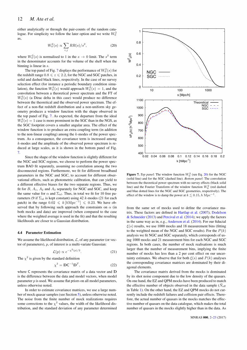
The top panel of Fig. 7 displays the performance ofW 20 (s) for
the redshift range 0.8 6 z 6 2.2, for the NGC and SGC patches, insolid and dashed black lines, respectively. In the case of no surveyselection effect (for instance a periodic boundary condition simu-lation), the function W 2
0 (s) would approach W 20 (s) = 1, and the
convolution between a theoretical power spectrum and the FT ofW 2
0 (s) (a Dirac delta in this case) would produce no differencebetween the theoretical and the observed power spectrum. The ef-fect of a non-flat redshift distribution and a non-uniform sky ge-ometry produces a window function with the shape observed inthe top panel of Fig. 7. As expected, the departure from the idealW 2
0 (s) = 1 case is more prominent in the SGC than in the NGS, asthe SGC footprint covers a smaller angular area. The effect of thewindow function is to produce an extra coupling term (in additionto the non-linear coupling) among the k-modes of the power spec-trum. As a consequence, the covariance term is increased amongk-modes and the amplitude of the observed power spectrum is re-duced at large scales, as it is shown in the bottom panel of Fig.7.
Since the shape of the window function is slightly different forthe NGC and SGC regions, we choose to perform the power spec-trum BAO fit separately, assuming no correlation among the twodisconnected regions. Furthermore, we fit for different broadbandparameters in the NGC and SGC, to account for different obser-vational effects, such as photometric calibration, that can yield toa different effective biases for the two separate regions. Thus, wefit for B, A1, A2 and A3 separately for NGC and SGC, and keepthe same value for α and Σnl. Thus, in total we fit for 10 free pa-rameters (9 if Σnl is kept constant) using 42 k-modes (21 for eachpatch) in the range 0.02 6 k [hMpc−1] 6 0.23. We have ob-served that by following such approach the constraints on α (inboth mocks and data) are improved (when compared to the casewhere the weighted average is used in the fit) and that the resultinglikelihoods are closer to a Gaussian distribution.
4.4 Parameter Estimation
We assume the likelihood distribution, L, of any parameter (or vec-tor of parameters), p, of interest is a multi-variate Gaussian:
L(p) ∝ e−χ2(p)/2. (21)
The χ2 is given by the standard definition
χ2 = DC−1DT , (22)
where C represents the covariance matrix of a data vector and Dis the difference between the data and model vectors, when modelparameter p is used. We assume flat priors on all model parameters,unless otherwise noted.
In order to estimate covariance matrices, we use a large num-ber of mock quasar samples (see Section 5), unless otherwise noted.The noise from the finite number of mock realizations requiressome corrections to the χ2 values, the width of the likelihood dis-tribution, and the standard deviation of any parameter determined
0
0.2
0.4
0.6
0.8
1
10 100 1000
W2 0(
s)
s [Mpc/h]
NGCSGC
400
500
600
700
800
900
1000
1100
0.02 0.04 0.06 0.08 0.1 0.12 0.14 0.16 0.18 0.2
kP0(
k) [h
-2M
pc2 ]
k [hMpc-1]
TheoreticalNGCSGC
Figure 7. Top panel: The window function W 20 (see Eq. 20) for the NGC
(solid line) and for the SGC (dashed line). Bottom panel: The convolutionbetween the theoretical power spectrum with no survey effects (black solidline) and the Fourier Transform of the window function W 2
0 (red dashedand blue dotted lines for the NGC and SGC geometries, respectively). Theeffect of the window is to damp the power at k . 0.15, h Mpc−1.
from the same set of mocks used to define the covariance ma-trix. These factors are defined in Hartlap et al. (2007); Dodelson& Schneider (2013) and Percival et al. (2014); we apply the factorsin the same way as in, e.g., Anderson et al. (2014). For our fiducialξ(s) results, we use 1000 mocks and 18 measurement bins (fittingto the weighted mean of the NGC and SGC results). For the P (k)analysis we fit NGC and SGC separately, which corresponds of us-ing 1000 mocks and 21 measurement bins for each NGC and SGCregions. In both cases, the number of mock realisations is muchlarger than the number of measurement bins, implying the finitenumber of mocks has less than a 2 per cent effect on our uncer-tainty estimates. We observe that for both ξ(s) and P (k) analysesthe corresponding covariance matrices are dominated by their di-agonal elements.
The covariance matrix derived from the mocks is dominatedby its shot noise component due to the low density of the quasars.On one hand, the EZ and QPM mocks have been produced to matchthe effective number of objects observed in the data sample (Neff
in Table 1). On the other hand, the EZ and QPM mocks do not cur-rently include the redshift failures and collision pair effects. There-fore, the actual number of quasars in the mocks matches the effec-tive number of quasars on the data catalogue, which makes the totalnumber of quasars in the mocks slightly higher than in the data. As
MNRAS 000, 2–23 (2017)

DR14 eBOSS Quasar BAO Measurements 13
a consequence, the diagonal and off-diagonal components of thecovariance are underestimated approximately by the ratio betweenNeff and NQ in the range 0.8 6 z 6 2.2. In order to correct forthis effect we re-scale the derived covariance elements by these fac-tors when analyzing the DR14 data, which are 1.069 for the NGCand 1.073 for the SGC. Future eBOSS analyses will include theseeffects in the mocks (and therefore this correction will be unneces-sary). Here, we use the simple scaling as it has only a 3 per centeffect on the recovered uncertainty.
5 SIMULATED CATALOGS
We use two different methods to create a total of 1400 simulationsof the DR14 quasar sample, which we refer to as ‘mocks’. In orderto create this number of mocks, approximate methods are required.Our approach in this respect is similar to previous BOSS analyses(Manera et al. 2013; Anderson et al. 2014; Alam et al. 2016). Thetwo methods used are ‘EZmock’ and ‘QPM’ and are described inthe following sub-sections.
5.1 EZmocks
For this work, we construct 1000 light-cone mock catalogues cov-ering the full survey area of DR14 (NGC+SGC) and reproducingthe redshift evolution of the observed quasar clustering. These arecreated using the ‘EZmock’ (Effective Zel’dovich approximationmock catalogue, Chuang et al. 2015a) method. EZmocks are con-structed using the Zel’dovich approximation of the density field.This approach accounts for non-linear effects and also halo bias(i.e. linear, nonlinear, deterministic, and stochastic bias) into aneffective modeling with few parameters, which can be efficientlycalibrated with observations or N-body simulations. Chuang et al.(2015b) demonstrates that the EZmock technique is able to pre-cisely reproduce the clustering of a given sample (including 2- and3-point statistics) with minimal computational resources, comparedto other methods. We use an improved version of EZmock codewith respect to the one described in Chuang et al. (2015a). In ourwork, we assign the positions of quasars to simulated dark matterparticles instead of populating them following a cloud-in-cell dis-tribution. With this change, we do not need to enhance the BAOsignal in the initial conditions, as done in Chuang et al. (2015a).
For this study, we calibrate the bias parameters with the ob-served DR14 eBOSS quasar clustering directly. The NGC and SGCregions are created from separate simulations and are treated inde-pendently, with bias values fit to the measured clustering and then(z) taken as in Fig. 1. Comparisons between the mean cluster-ing in the EZmock samples and the measured eBOSS clusteringcan be found in Figs. 5 and 6, demonstrating that a good matchhas been produced. The EZmocks use the same initial power spec-trum used by the mock catalogues of the final BOSS data release(DR12; Kitaura et al. 2016; Alam et al. 2016). The fiducial cosmol-ogy model is ΛCDM with Ωm=0.307115, h=0.6777, σ8=0.8225,Ωb=0.048206, ns=0.9611 (see Kitaura et al. 2016 for details).
Each light-cone mock constructed for this work is composedof 7 redshift shells. The redshift shells for a given light-cone mockare computed using different EZmock parameters but they sharethe same initial Gaussian density field so that the background den-sity field is continuous. Each redshift shell is taken from one corre-sponding EZmock periodic box with the size of (5h−1Gpc)3. Forthis study, we generated 1000×7(shells)×2(NGC+SGC)=14,000EZmock boxes in total. We use the code make survey Carlson &
0.50 0.75 1.00 1.25 1.50 1.75 2.00 2.25 2.50
z
1.0
1.5
2.0
2.5
3.0
3.5
4.0
4.5
b(z)
EZmocks
Croom et al. 2005
Laurent et al. 2017
Figure 8. We compare the linear bias measured from EZmocks used inthis work with the other measurements from observed data (Croom et al.2005; Laurent et al. 2017). The bias evolution in the EZmocks is in goodagreement with these works.
White (2010); White et al. (2014) to construct each redshift shellfrom the corresponding box.
In order to determine the redshift evolution of each EZmockparameter, we need to measure/determine the parameters at dif-ferent redshifts. However, the clustering measurements from theobservation corresponding to each redshift shell are too noisy tobe used to determine the EZmock parameter values. Therefore, weuse samples from overlapping redshift bins to measure the EZmockparameters at different redshift and do a proper inter- or extra- po-lation to determine the parameters for all the 7 redshift shells. Foreach EZmock parameter p, we assume that its functional depen-dency is well approximated by
p = c0 + c1Z(1) + c2Z(2), (23)
where
Z(i) =
∑zmin6zj<zmax
N(zj)zji
∑zmin6zj<zmax
N(zj), i = 1, 2, (24)
of the number count N(zj) within a given redshift bin zj (with binsize ∆z = 0.01).
For this work, we measured the EZmock parameters from ob-servation in the following three redshift ranges: 0.8 6 z1 < 1.5,1.2 6 z2 < 1.8, and 1.5 6 z3 < 2.2, respectively. We determinethe c0, c1, and c2 by solving the following equations
p1 = c0 + c1Z1(1) + c2Z1(2),
p2 = c0 + c1Z2(1) + c2Z2(2),
p3 = c0 + c1Z3(1) + c2Z3(2). (25)
Having solved the system of Eqs. 25 for the coefficients c0, c1and c2, Eq. 23 is used to determine an EZmock parameter value forany given redshift shell.
MNRAS 000, 2–23 (2017)
14 M. Ata et al.
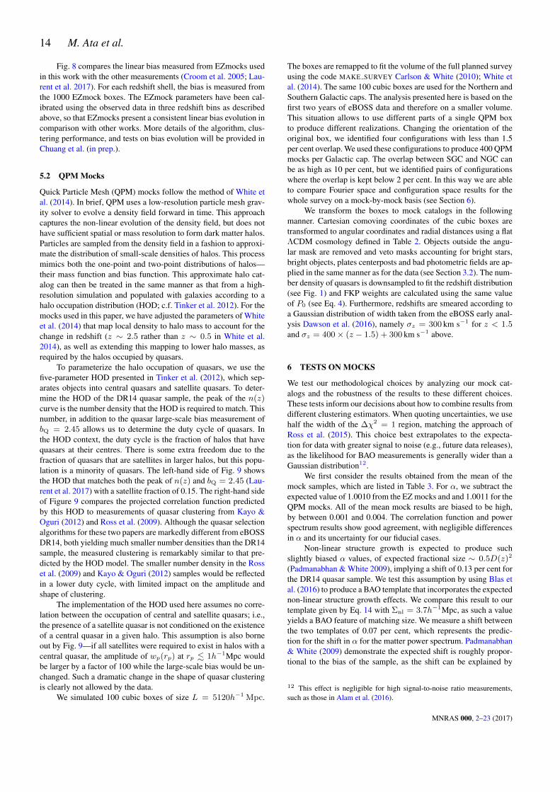
Fig. 8 compares the linear bias measured from EZmocks usedin this work with the other measurements (Croom et al. 2005; Lau-rent et al. 2017). For each redshift shell, the bias is measured fromthe 1000 EZmock boxes. The EZmock parameters have been cal-ibrated using the observed data in three redshift bins as describedabove, so that EZmocks present a consistent linear bias evolution incomparison with other works. More details of the algorithm, clus-tering performance, and tests on bias evolution will be provided inChuang et al. (in prep.).
5.2 QPM Mocks
Quick Particle Mesh (QPM) mocks follow the method of White etal. (2014). In brief, QPM uses a low-resolution particle mesh grav-ity solver to evolve a density field forward in time. This approachcaptures the non-linear evolution of the density field, but does nothave sufficient spatial or mass resolution to form dark matter halos.Particles are sampled from the density field in a fashion to approxi-mate the distribution of small-scale densities of halos. This processmimics both the one-point and two-point distributions of halos—their mass function and bias function. This approximate halo cat-alog can then be treated in the same manner as that from a high-resolution simulation and populated with galaxies according to ahalo occupation distribution (HOD; c.f. Tinker et al. 2012). For themocks used in this paper, we have adjusted the parameters of Whiteet al. (2014) that map local density to halo mass to account for thechange in redshift (z ∼ 2.5 rather than z ∼ 0.5 in White et al.2014), as well as extending this mapping to lower halo masses, asrequired by the halos occupied by quasars.
To parameterize the halo occupation of quasars, we use thefive-parameter HOD presented in Tinker et al. (2012), which sep-arates objects into central quasars and satellite quasars. To deter-mine the HOD of the DR14 quasar sample, the peak of the n(z)curve is the number density that the HOD is required to match. Thisnumber, in addition to the quasar large-scale bias measurement ofbQ = 2.45 allows us to determine the duty cycle of quasars. Inthe HOD context, the duty cycle is the fraction of halos that havequasars at their centres. There is some extra freedom due to thefraction of quasars that are satellites in larger halos, but this popu-lation is a minority of quasars. The left-hand side of Fig. 9 showsthe HOD that matches both the peak of n(z) and bQ = 2.45 (Lau-rent et al. 2017) with a satellite fraction of 0.15. The right-hand sideof Figure 9 compares the projected correlation function predictedby this HOD to measurements of quasar clustering from Kayo &Oguri (2012) and Ross et al. (2009). Although the quasar selectionalgorithms for these two papers are markedly different from eBOSSDR14, both yielding much smaller number densities than the DR14sample, the measured clustering is remarkably similar to that pre-dicted by the HOD model. The smaller number density in the Rosset al. (2009) and Kayo & Oguri (2012) samples would be reflectedin a lower duty cycle, with limited impact on the amplitude andshape of clustering.
The implementation of the HOD used here assumes no corre-lation between the occupation of central and satellite quasars; i.e.,the presence of a satellite quasar is not conditioned on the existenceof a central quasar in a given halo. This assumption is also borneout by Fig. 9—if all satellites were required to exist in halos with acentral quasar, the amplitude of wp(rp) at rp . 1h−1Mpc wouldbe larger by a factor of 100 while the large-scale bias would be un-changed. Such a dramatic change in the shape of quasar clusteringis clearly not allowed by the data.
We simulated 100 cubic boxes of size L = 5120h−1 Mpc.
The boxes are remapped to fit the volume of the full planned surveyusing the code MAKE SURVEY Carlson & White (2010); White etal. (2014). The same 100 cubic boxes are used for the Northern andSouthern Galactic caps. The analysis presented here is based on thefirst two years of eBOSS data and therefore on a smaller volume.This situation allows to use different parts of a single QPM boxto produce different realizations. Changing the orientation of theoriginal box, we identified four configurations with less than 1.5per cent overlap. We used these configurations to produce 400 QPMmocks per Galactic cap. The overlap between SGC and NGC canbe as high as 10 per cent, but we identified pairs of configurationswhere the overlap is kept below 2 per cent. In this way we are ableto compare Fourier space and configuration space results for thewhole survey on a mock-by-mock basis (see Section 6).
We transform the boxes to mock catalogs in the followingmanner. Cartesian comoving coordinates of the cubic boxes aretransformed to angular coordinates and radial distances using a flatΛCDM cosmology defined in Table 2. Objects outside the angu-lar mask are removed and veto masks accounting for bright stars,bright objects, plates centerposts and bad photometric fields are ap-plied in the same manner as for the data (see Section 3.2). The num-ber density of quasars is downsampled to fit the redshift distribution(see Fig. 1) and FKP weights are calculated using the same valueof P0 (see Eq. 4). Furthermore, redshifts are smeared according toa Gaussian distribution of width taken from the eBOSS early anal-ysis Dawson et al. (2016), namely σz = 300 km s−1 for z < 1.5and σz = 400× (z − 1.5) + 300 km s−1 above.
6 TESTS ON MOCKS
We test our methodological choices by analyzing our mock cat-alogs and the robustness of the results to these different choices.These tests inform our decisions about how to combine results fromdifferent clustering estimators. When quoting uncertainties, we usehalf the width of the ∆χ2 = 1 region, matching the approach ofRoss et al. (2015). This choice best extrapolates to the expecta-tion for data with greater signal to noise (e.g., future data releases),as the likelihood for BAO measurements is generally wider than aGaussian distribution12.
We first consider the results obtained from the mean of themock samples, which are listed in Table 3. For α, we subtract theexpected value of 1.0010 from the EZ mocks and and 1.0011 for theQPM mocks. All of the mean mock results are biased to be high,by between 0.001 and 0.004. The correlation function and powerspectrum results show good agreement, with negligible differencesin α and its uncertainty for our fiducial cases.
Non-linear structure growth is expected to produce suchslightly biased α values, of expected fractional size ∼ 0.5D(z)2
(Padmanabhan & White 2009), implying a shift of 0.13 per cent forthe DR14 quasar sample. We test this assumption by using Blas etal. (2016) to produce a BAO template that incorporates the expectednon-linear structure growth effects. We compare this result to ourtemplate given by Eq. 14 with Σnl = 3.7h−1Mpc, as such a valueyields a BAO feature of matching size. We measure a shift betweenthe two templates of 0.07 per cent, which represents the predic-tion for the shift in α for the matter power spectrum. Padmanabhan& White (2009) demonstrate the expected shift is roughly propor-tional to the bias of the sample, as the shift can be explained by
12 This effect is negligible for high signal-to-noise ratio measurements,such as those in Alam et al. (2016).
MNRAS 000, 2–23 (2017)

DR14 eBOSS Quasar BAO Measurements 15
Figure 9. Left panel: The mean halo occupation of quasars used in the QPM mocks. The solid red curve shows the mean number of central quasars per halo,while the blue dashed curve indicates the mean number of satellite quasars per halo. The horizontal asymptote of 0.01 central quasars per halo reflects theadopted duty cycle of 1% for quasars in the eBOSS sample. The number of central and satellite quasars in a halo are uncorrelated with one another; i.e., thepresence of a satellite quasar is not conditioned on the existence of a central quasar. Right panel: The projected correlation function, wp(rp), yielded by theHOD in the left panel. For comparison, the red squares are the measurement of wp(rp) of quasars from Kayo & Oguri (2012), while the blue circles representthe measurements from Ross et al. (2009). The solid curve is calculated from the theoretical HOD model of Tinker et al. (2012).
higher-order bias terms and these for dark matter halos are roughlyproportional to the linear bias. Given that Laurent et al. (2017) ob-tains a bias of 2.45 for eBOSS quasars, we should expect roughly0.2 per cent shifts in the α recovered from our fiducial template(which includes no shifts due to non-linear structure growth). Thisprediction is generally consistent with our results when using themean of the mocks. The differences in these tests, compared withthe expected α, are at most 2σ in terms of the ensemble of mocksbeing tested and never more than 0.1σ compared to the expected re-sult for a single realization. We thus consider any potential bias dueto non-linear structure growth to be negligible given the uncertaintyobtained from the DR14 quasar sample.
In order to test the effect of redshift uncertainties, we have runthe QPM mocks with a variety of assumptions on the redshift un-certainty; full details can be found in Zarrouk et al. (in prep.). Wesimply consider the fiducial case, with redshift uncertainty match-ing Fig. 11 of Dawson et al. (2016) and a case without any redshiftuncertainty. Without any redshift uncertainty, the mean ξ(s) of theQPM mocks is best-fit by Σnl = 3.7h−1Mpc; with the redshiftuncertainty, the best-fit is Σnl = 5.5h−1Mpc. These results sug-gest our choice to use Σnl = 6.0h−1Mpc is slightly conservative(greater Σnl leads to a greater uncertainty obtained from the likeli-hood).
Table 4 displays the results obtained when fitting each indi-vidual mock. Here, we only report statistics for mocks that have a∆χ2 = 1 on both sides of the minimum χ2, within our prior rangeof 0.8 < α < 1.2. We designate each such mock result a ‘detec-tion’. Over 90 per cent of the mock samples satisfy this condition.For this reason, the mean σs are slightly less than that obtained forthe mean of the mock realizations (multiplying the uncertainty inTable 3 by
√Nmock). The standard deviation of these samples is
close to the mean uncertainty, as would be expected for a Gaussiandistribution.
Table 3. Tests of BAO fits on the mean of the quasar mocks. Fiducialresults use the EZmocks for the covariance matrix, ∆s = 8h−1Mpc;35 < s < 180h−1Mpc for ξ(s), and evenly-spaced ∆k = 0.01hMpc−1;0.02 < k < 0.23hMpc−1 for P (k). The uncertainties are those for thefull ensemble, e.g., one with 1000 (400) times the size of a single EZ (QPM)mock. The EZmock and QPM results are independent, but results using thesame set of mocks are highly correlated. A small positive bias is expectedfrom non-linear structure growth, see text for details.
case α− αexp
EZ mocks:ξ(s):
fiducial 0.0023± 0.0016
5h−1Mpc 0.0027± 0.0016P (k):
fiducial 0.0019± 0.0017
kmax = 0.30hMpc−1 0.0009± 0.0017Σnl = [6± 3]h−1Mpc 0.0021± 0.0016
Σnl = [6± 3]h−1Mpc & kmax = 0.30 0.0011± 0.0016logk - binning 0.0032± 0.0017logk - binning & kmax = 0.30hMpc−1 0.0022± 0.0016A4, A5 terms 0.0037± 0.0017
QPM mocks:ξ(s):
fiducial 0.0017± 0.00285h−1Mpc 0.0027± 0.0028
QPM cov 0.0023± 0.0026P (k):
fiducial 0.0017± 0.0027
QPM cov 0.0012± 0.0026
MNRAS 000, 2–23 (2017)

16 M. Ata et al.
Table 4. Statistics for BAO fits on EZ and QPM mocks. 〈α〉 is the meanmeasured BAO parameter with 1σ bounds within the range 0.8 < α < 1.2.〈σ〉 is the same for the uncertainty obtained from ∆χ2 = 1 region and Sis the standard deviation of these α. Ndet is the number of realizationswith such 1σ bounds. Both EZmocks and QPMmocks were created witha slightly different cosmology than our fiducial assumed cosmology. Thus,for the EZmocks, the expected α values are 1.0010; and for QPM 1.0011.The ξ bin size is 8h−1Mpc, unless noted otherwise. Tests of shifting bincentres are noted by +x, with x representing the shift in h−1Mpc. Thedamping is Σnl = 6h−1Mpc, unless otherwise noted. The binning forP (k) is linear spaced in 0.01hMpc−1, unless otherwise noted. As for ξ,test of shifting bin centres are noted by +x/4, with x/4 representing theshift in fractions of the k-bin size. The EZmock and QPM results are in-dependent, but results using the same set of mocks are highly correlated. Asmall positive bias is expected from non-linear structure growth, see text fordetails.
case (+bin shift) 〈α〉 〈σ〉 S Ndet/Ntot
EZ mocks:consensus P (k) + ξ(s) 1.003 0.050 0.050 944/1000ξ(s):
combined 1.003 0.049 0.049 939/1000fiducial 1.002 0.048 0.050 932/1000+2 1.002 0.049 0.050 928/1000+4 1.002 0.048 0.050 938/1000+6 1.003 0.048 0.051 929/10005h−1Mpc 1.003 0.049 0.050 937/1000
P (k):combined 1.002 0.052 0.050 941/1000fiducial 1.002 0.051 0.051 929/1000+1/4 1.001 0.052 0.050 931/1000+2/4 1.004 0.051 0.049 935/1000+3/4 1.001 0.052 0.050 937/1000logk - binning 1.002 0.051 0.050 927/1000kmax = 0.30hMpc−1 1.002 0.051 0.051 934/1000
QPM mocks:ξ(s):
fiducial 1.001 0.051 0.052 361/4005h−1Mpc 1.000 0.050 0.051 355/400QPM cov 1.002 0.051 0.052 369/400P (k):
fiducial 0.998 0.049 0.051 354/400QPM cov 0.999 0.049 0.049 359/400
For the correlation function, the mean α values are similar tothose obtained when testing the mean of the mocks, as expected.We test bin sizes of 5h−1Mpc and 8h−1Mpc; the results are ex-tremely similar and we thus choose 8h−1Mpc binning as it rep-resents the smaller data vector. The QPM and EZ mocks produceconsistent results, suggesting the separate methods agree on the ex-pected BAO signal-to-noise ratio in our DR14 quasar sample. Inparticular, the results for the QPM mocks are insensitive to whetherwe use the QPM mocks or the EZ mocks to construct the covari-ance matrix used for the fits. This suggests our results are robust touncertainties in how we construct the covariance matrix.
For 8h−1Mpc correlation function binning, results using dif-ferent bin centres are not perfectly correlated. Instead, the corre-lation factors, when shifting by each available 2h−1Mpc shift, areclose to 0.9 (the range is 0.88 to 0.92). Thus, slightly improvedresults are obtained when combining the results of these four bincentres; for Gaussian distributions, we would expect a 4 per centimprovement given four measurements with correlation 0.9. We
combine the results by simply taking the mean of the four likeli-hoods, matching the approach of Ross et al. (2015). This combi-nation increases the number of detections from 932 to 939 and re-duces the standard deviation from 0.050 to 0.049. These results arelabeled ‘combined’ in Table 4 and represent our optimized methodfor measuring the correlation function BAO scale.
We find broadly consistent results in Fourier space. The fidu-cial power spectrum case recovers essentially the same number ofdetections (929 compared to 932) and has a slightly larger mean un-certainty and standard deviation. We test four bin centres for P (k),shifting the centre by factors of 0.025kMpc−1. These results aremore correlated than the ξ(s) bin centre results, as they range 0.94and 0.96. Combining across the bin centre results by taking themean of the four likelihoods increases the number of detectionsto 941 while keeping the mean uncertainty and standard deviationunchanged. The power spectrum results are consistent whether theQPM or EZ mocks are being tested, whether a logarithmic or lineark-space binning is used, and whether the maximum k-vector forthe analysis is set to 0.23 or 0.30hMpc−1.
We compare the P (k) and ξ(s) results directly for the caseswhere we averaged across the bin centres for the EZmocks (denoted‘combined’ in Table 4). The recovered α are plotted against eachother in the top panel Fig. 10, using steelblue circles. The resultsare strongly correlated (the correlation factor is 0.97) and are un-biased relative to each other. The bottom panel in Fig. 10 displaysthe uncertainty of the combined P (k) and ξ(s) results. The uncer-tainties are not as correlated as the best-fit α, as the uncertaintiesobtained from the P (k) likelihoods are more narrowly distributedthan the ξ(s) counterparts.
Given that the combined P (k) and ξ(s) produce slightly dif-ferent likelihoods, but with strong correlation in the maximum like-lihood, we adopt the mean of the P (k) and ξ(s) results as a ‘con-sensus’ measurement. Doing so, we obtain a slight increase in thenumber of detections (up to 944) and the standard deviation in themaximum likelihood value of α matches the mean uncertainty ob-tained from the likelihood. Further, (α − 〈α〉)/σ(α) is distributedsimilarly to a unit Gaussian distribution, as shown in Fig. 11. Theseresults suggest that the uncertainty we obtain by combining theP (k) and ξ(s) likelihoods are indeed good estimates of the un-certainty on α for each mock realization. We copy this approachwhen obtaining our consensus results using the DR14 quasar data.
The tests presented in this Section define our procedure forobtaining BAO measurements from the data. The results suggestthat there are no reasonable methodological choices that will affectour estimate of the uncertainty on our measurements by more than10 per cent or bias our results by more than 0.1σ.
7 RESULTS
7.1 Clustering Measurements
We measure the clustering of the DR14 quasar sample in the re-spective SGC and NGC regions, i.e., the window function is nor-malized in each respective region, and then the results are com-bined. In this section, we present the clustering measurements, inboth configuration and Fourier space, comparing the results to eachother and to the mock DR14 samples.
Fig. 5 displays the spherically averaged redshift-space corre-lation function of the DR14 quasar sample for the data in the SGC(blue squares) and NGC (red diamonds). The dashed curves displaythe mean of the 1000 EZmock samples. The data in each region
MNRAS 000, 2–23 (2017)
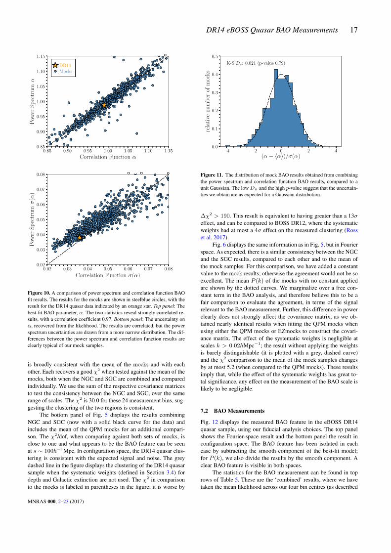
DR14 eBOSS Quasar BAO Measurements 17
0.85 0.90 0.95 1.00 1.05 1.10 1.15
Correlation Function α
0.85
0.90
0.95
1.00
1.05
1.10
1.15
Pow
erS
pec
tru
mα
DR14
Mocks
0.02 0.03 0.04 0.05 0.06 0.07 0.08
Correlation Function σ(α)
0.02
0.03
0.04
0.05
0.06
0.07
0.08
Pow
erS
pec
tru
mσ
(α)
Figure 10. A comparison of power spectrum and correlation function BAOfit results. The results for the mocks are shown in steelblue circles, with theresult for the DR14 quasar data indicated by an orange star. Top panel: Thebest-fit BAO parameter, α. The two statistics reveal strongly correlated re-sults, with a correlation coefficient 0.97. Bottom panel: The uncertainty onα, recovered from the likelihood. The results are correlated, but the powerspectrum uncertainties are drawn from a more narrow distribution. The dif-ferences between the power spectrum and correlation function results areclearly typical of our mock samples.
is broadly consistent with the mean of the mocks and with eachother. Each recovers a good χ2 when tested against the mean of themocks, both when the NGC and SGC are combined and comparedindividually. We use the sum of the respective covariance matricesto test the consistency between the NGC and SGC, over the samerange of scales. The χ2 is 30.0 for these 24 measurement bins, sug-gesting the clustering of the two regions is consistent.
The bottom panel of Fig. 5 displays the results combiningNGC and SGC (now with a solid black curve for the data) andincludes the mean of the QPM mocks for an additional compari-son. The χ2/dof, when comparing against both sets of mocks, isclose to one and what appears to be the BAO feature can be seenat s ∼ 100h−1Mpc. In configuration space, the DR14 quasar clus-tering is consistent with the expected signal and noise. The greydashed line in the figure displays the clustering of the DR14 quasarsample when the systematic weights (defined in Section 3.4) fordepth and Galactic extinction are not used. The χ2 in comparisonto the mocks is labeled in parentheses in the figure; it is worse by
−4 −2 0 2 4(α− 〈α〉)/σ(α)
0.0
0.1
0.2
0.3
0.4
0.5
rela
tive
num
ber
ofm
ocks
K-S Dn: 0.021 (p-value 0.79)
Figure 11. The distribution of mock BAO results obtained from combiningthe power spectrum and correlation function BAO results, compared to aunit Gaussian. The lowDn and the high p-value suggest that the uncertain-ties we obtain are as expected for a Gaussian distribution.
∆χ2 > 190. This result is equivalent to having greater than a 13σeffect, and can be compared to BOSS DR12, where the systematicweights had at most a 4σ effect on the measured clustering (Rosset al. 2017).
Fig. 6 displays the same information as in Fig. 5, but in Fourierspace. As expected, there is a similar consistency between the NGCand the SGC results, compared to each other and to the mean ofthe mock samples. For this comparison, we have added a constantvalue to the mock results; otherwise the agreement would not be soexcellent. The mean P (k) of the mocks with no constant appliedare shown by the dotted curves. We marginalize over a free con-stant term in the BAO analysis, and therefore believe this to be afair comparison to evaluate the agreement, in terms of the signalrelevant to the BAO measurement. Further, this difference in powerclearly does not strongly affect the covariance matrix, as we ob-tained nearly identical results when fitting the QPM mocks whenusing either the QPM mocks or EZmocks to construct the covari-ance matrix. The effect of the systematic weights is negligible atscales k > 0.02hMpc−1; the result without applying the weightsis barely distinguishable (it is plotted with a grey, dashed curve)and the χ2 comparison to the mean of the mock samples changesby at most 5.2 (when compared to the QPM mocks). These resultsimply that, while the effect of the systematic weights has great to-tal significance, any effect on the measurement of the BAO scale islikely to be negligible.
7.2 BAO Measurements
Fig. 12 displays the measured BAO feature in the eBOSS DR14quasar sample, using our fiducial analysis choices. The top panelshows the Fourier-space result and the bottom panel the result inconfiguration space. The BAO feature has been isolated in eachcase by subtracting the smooth component of the best-fit model;for P (k), we also divide the results by the smooth component. Aclear BAO feature is visible in both spaces.
The statistics for the BAO measurement can be found in toprows of Table 5. These are the ‘combined’ results, where we havetaken the mean likelihood across our four bin centres (as described
MNRAS 000, 2–23 (2017)
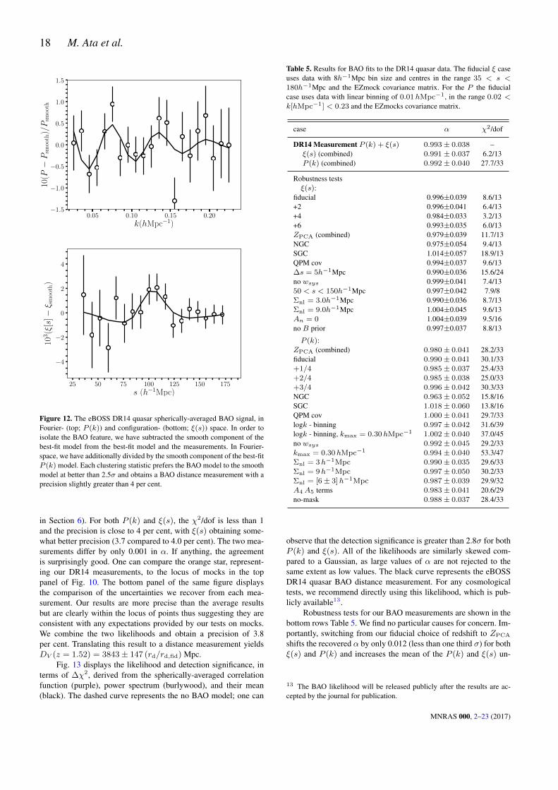
18 M. Ata et al.
0.05 0.10 0.15 0.20
k(hMpc−1)
−1.5
−1.0
−0.5
0.0
0.5
1.0
1.5
10(P−P
smoot
h)/P
smoot
h
25 50 75 100 125 150 175
s (h−1Mpc)
−4
−2
0
2
4
103(ξ
[s]−
ξ sm
oot
h)
Figure 12. The eBOSS DR14 quasar spherically-averaged BAO signal, inFourier- (top; P (k)) and configuration- (bottom; ξ(s)) space. In order toisolate the BAO feature, we have subtracted the smooth component of thebest-fit model from the best-fit model and the measurements. In Fourier-space, we have additionally divided by the smooth component of the best-fitP (k) model. Each clustering statistic prefers the BAO model to the smoothmodel at better than 2.5σ and obtains a BAO distance measurement with aprecision slightly greater than 4 per cent.
in Section 6). For both P (k) and ξ(s), the χ2/dof is less than 1and the precision is close to 4 per cent, with ξ(s) obtaining some-what better precision (3.7 compared to 4.0 per cent). The two mea-surements differ by only 0.001 in α. If anything, the agreementis surprisingly good. One can compare the orange star, represent-ing our DR14 measurements, to the locus of mocks in the toppanel of Fig. 10. The bottom panel of the same figure displaysthe comparison of the uncertainties we recover from each mea-surement. Our results are more precise than the average resultsbut are clearly within the locus of points thus suggesting they areconsistent with any expectations provided by our tests on mocks.We combine the two likelihoods and obtain a precision of 3.8per cent. Translating this result to a distance measurement yieldsDV (z = 1.52) = 3843± 147 (rd/rd,fid) Mpc.
Fig. 13 displays the likelihood and detection significance, interms of ∆χ2, derived from the spherically-averaged correlationfunction (purple), power spectrum (burlywood), and their mean(black). The dashed curve represents the no BAO model; one can
Table 5. Results for BAO fits to the DR14 quasar data. The fiducial ξ caseuses data with 8h−1Mpc bin size and centres in the range 35 < s <180h−1Mpc and the EZmock covariance matrix. For the P the fiducialcase uses data with linear binning of 0.01hMpc−1, in the range 0.02 <
k[hMpc−1] < 0.23 and the EZmocks covariance matrix.
case α χ2/dof
DR14 Measurement P (k) + ξ(s) 0.993± 0.038 –ξ(s) (combined) 0.991± 0.037 6.2/13P (k) (combined) 0.992± 0.040 27.7/33
Robustness testsξ(s):
fiducial 0.996±0.039 8.6/13+2 0.996±0.041 6.4/13+4 0.984±0.033 3.2/13+6 0.993±0.035 6.0/13ZPCA (combined) 0.979±0.039 11.7/13NGC 0.975±0.054 9.4/13SGC 1.014±0.057 18.9/13QPM cov 0.994±0.037 9.6/13∆s = 5h−1Mpc 0.990±0.036 15.6/24no wsys 0.999±0.041 7.4/1350 < s < 150h−1Mpc 0.997±0.042 7.9/8Σnl = 3.0h−1Mpc 0.990±0.036 8.7/13Σnl = 9.0h−1Mpc 1.004±0.045 9.6/13An = 0 1.004±0.039 9.5/16no B prior 0.997±0.037 8.8/13
P (k):ZPCA (combined) 0.980± 0.041 28.2/33fiducial 0.990± 0.041 30.1/33+1/4 0.985± 0.037 25.4/33+2/4 0.985± 0.038 25.0/33+3/4 0.996± 0.042 30.3/33NGC 0.963± 0.052 15.8/16SGC 1.018± 0.060 13.8/16QPM cov 1.000± 0.041 29.7/33logk - binning 0.997± 0.042 31.6/39logk - binning, kmax = 0.30hMpc−1 1.002± 0.040 37.0/45no wsys 0.992± 0.045 29.2/33kmax = 0.30hMpc−1 0.994± 0.040 53.3/47Σnl = 3h−1Mpc 0.990± 0.035 29.6/33Σnl = 9h−1Mpc 0.997± 0.050 30.2/33Σnl = [6± 3]h−1Mpc 0.987± 0.039 29.9/32A4 A5 terms 0.983± 0.041 20.6/29no-mask 0.988± 0.037 28.4/33
observe that the detection significance is greater than 2.8σ for bothP (k) and ξ(s). All of the likelihoods are similarly skewed com-pared to a Gaussian, as large values of α are not rejected to thesame extent as low values. The black curve represents the eBOSSDR14 quasar BAO distance measurement. For any cosmologicaltests, we recommend directly using this likelihood, which is pub-licly available13.
Robustness tests for our BAO measurements are shown in thebottom rows Table 5. We find no particular causes for concern. Im-portantly, switching from our fiducial choice of redshift to ZPCA
shifts the recovered α by only 0.012 (less than one third σ) for bothξ(s) and P (k) and increases the mean of the P (k) and ξ(s) un-
13 The BAO likelihood will be released publicly after the results are ac-cepted by the journal for publication.
MNRAS 000, 2–23 (2017)

DR14 eBOSS Quasar BAO Measurements 19
0.8 0.9 1.0 1.1 1.2αBAO
0
2
4
6
8
10
12
14
16
∆χ
2
1σ
2σ
3σ
ξ(s)P (k)P (k) + ξ(s)
Figure 13. The solid curve displays the likelihood of the BAO parameterα, in terms of ∆χ2, recovered from the spherically averaged correlationfunction of the DR14 quasar sample. The dashed curve displays the sameinformation for a no BAO model, where ∆χ2 is determined by subtractingthe minimumχ2 from the BAO model. The detection significance is slightlyless than 3σ and the likelihood is slightly skewed compared to the Gaussianexpectation. The purple curve displays correlation function results and theburlywood curve displays the power spectrum result. The black curve is themean of the two likelihoods, which is what we use as our final measurement.
certainty from 0.038 to 0.040. These results have been combinedacross bin centres and can be compared directly to the DR14 re-sults on the top lines of the table. The choice of redshift techniqueclearly does not have a strong impact on our results. Zarrouk etal. (in prep.) will examine this issue more closely in the contextof RSD measurements, but we note that, e.g., we find no clear dif-ferences in the linear bias or excess large-scale clustering obtainedusing either redshift.
Additional robustness tests should be compared to the ‘fidu-cial’ results, which are the results for the fiducial choice of bincentre. The variations with bin centre for ξ(s) (labeled +x) andP (k) (labeled +x/4) are consistent with our findings testing ourresults with mocks; the mean of these four likelihoods is used asthe DR14 ξ(s) measurement, labeled ‘combined’ in the top rows.Additional tests produce no changes that are greater than 0.2σ forξ(s). For P (k), the greatest change is only 0.3σ when switching tologarithmic binning and increasing kmax to 0.3hMpc−1. Finally,the results obtained from the independent NGC and SGC regionsagree within 1σ, for both ξ(s) and P (k)
The systematic weights have negligible effects on our mea-surements, despite their enormous (13σ) effect on the large-scalecorrelation function of the DR14 quasar sample. We simply recoverless than a 0.1σ shift in α and a 5 per cent increase in the uncer-tainty. The χ2 of the best-fit actually decreases (by 1), suggestingthe effect of the depth and extinction systematics on our correlationfunction measurements are trivially accounted for with the polyno-mial terms in our BAO model.
For both ξ(s) and P (k), there is a slight correlation betweenthe assumed Σnl and the recovered α that is less than ∼0.2σ whentesting in the range ±3.0h1Mpc around our fiducial choice, with asimilar impact on the size of the recovered uncertainty. For P (k),we are able to marginalize over this parameter in the fit (usinga Gaussian prior of ±3.0h1Mpc) and we recover a result thatmatches the fiducial result with Σnl fixed at 6.0h1Mpc to better
0.0 0.5 1.0 1.5 2.0 2.5
Redshift
0.95
1.00
1.05
Dis
tan
ce/D
ista
nce
(Pla
nck
ΛC
DM
)
6dFGSBOSS DR12
SDSS MGS
WiggleZDR14 quasars
BOSS Lyα
Figure 14. Spherically averaged BAO distance measurements (DV ) com-pared to the Planck ΛCDM prediction and extrapolated 68 per cent CL(grey region). The eBOSS DR14 quasar sample measurement is shown us-ing a gold star. The additional measurements are described in the text.
than 0.1σ. Thus, not only does the choice of Σnl have a minor ef-fect on our analysis, our choice for its fiducial value is sufficientlyclose to the best-fit value as to not make a difference in our results.
Overall, the robustness tests suggest that our results are in-sensitive to arbitrary choices in the analysis or the way the catalogwas constructed. This is consistent with Ross et al. (2017); Vargas-Magana et al. (2016) who showed that systematic uncertainties aresmall compared to the BOSS DR12 statistical uncertainties. TheBOSS DR12 precision is a factor of four better than our own, andthus makes these systematic uncertainties negligibly small for ouranalysis. A separate systematic uncertainty is the possible shift inthe acoustic peak due to a coupling of the quasar density field tothe small relative velocity between baryons and cold dark matterat high redshift (Tseliakhovich & Hirata 2010; Dalal et al. 2010;Yoo et al. 2011; Slepian & Eisenstein 2015; Blazek et al. 2016;Schmidt 2016). This has been shown to be less than 0.5 per cent forlow redshift galaxies (Yoo et al. 2013; Beutler et al. 2016; Slepianet al. 2016) and we expect it to be a minor effect for quasars withz ∼ 1.5, compared to our statistical uncertainty. Further study iswarranted, especially as the statistical uncertainty will be consider-ably improved with future datasets.
8 COSMOLOGICAL IMPLICATIONS
In this section, we briefly discuss the cosmological implicationsof our DR14 quasar BAO measurement of DV (z = 1.52) =3843± 147 (rd/rd,fid) Mpc. We first present an updated BAO dis-tance ladder and then demonstrate how this BAO distance ladderalone provides a powerful constraint on the geometry of the Uni-verse.
Fig. 14 displays our spherically averaged BAO measurementsoverplotted with the ΛCDM prediction from Planck (Planck Col-laboration et al. 2015), compared to various similar measurementsin the literature: the 6dFGS result from Beutler et al. (2011), theSDSS MGS result from Ross et al. (2015), the BOSS DR12 re-sults from Alam et al. (2016), the WiggleZ results from Kazin et al.(2014), and the BOSS Lyα from the combination of the Bautistaet al. (2017) DR12 Lyα auto-correlation and the Font-Ribera et al.
MNRAS 000, 2–23 (2017)
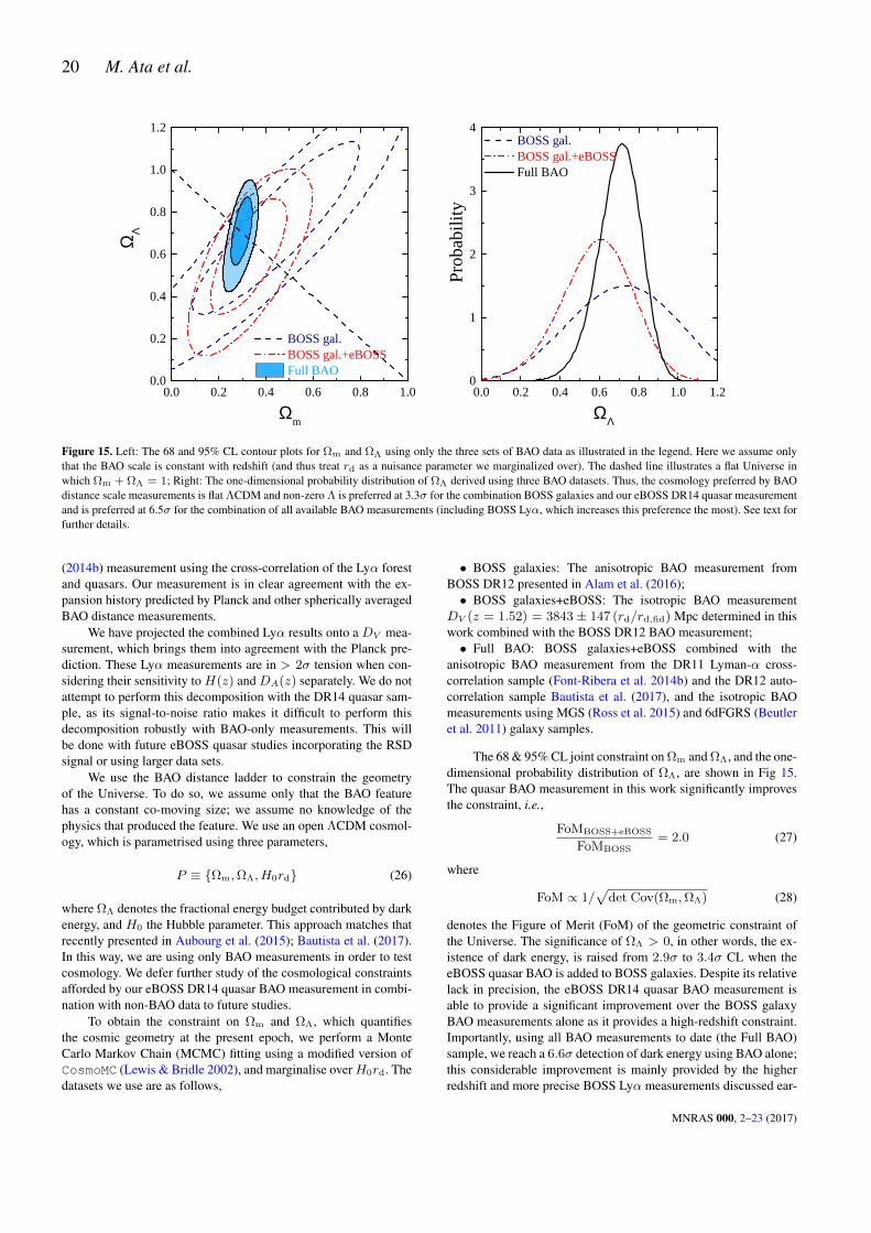
20 M. Ata et al.
0 . 0 0 . 2 0 . 4 0 . 6 0 . 8 1 . 00 . 0
0 . 2
0 . 4
0 . 6
0 . 8
1 . 0
1 . 2
B O S S g a l . B O S S g a l . + e B O S S F u l l B A O
Ω
Λ
Ωm
0 . 0 0 . 2 0 . 4 0 . 6 0 . 8 1 . 0 1 . 20
1
2
3
4
Probab
ility
ΩΛ
B O S S g a l . B O S S g a l . + e B O S S F u l l B A O
Figure 15. Left: The 68 and 95% CL contour plots for Ωm and ΩΛ using only the three sets of BAO data as illustrated in the legend. Here we assume onlythat the BAO scale is constant with redshift (and thus treat rd as a nuisance parameter we marginalized over). The dashed line illustrates a flat Universe inwhich Ωm + ΩΛ = 1; Right: The one-dimensional probability distribution of ΩΛ derived using three BAO datasets. Thus, the cosmology preferred by BAOdistance scale measurements is flat ΛCDM and non-zero Λ is preferred at 3.3σ for the combination BOSS galaxies and our eBOSS DR14 quasar measurementand is preferred at 6.5σ for the combination of all available BAO measurements (including BOSS Lyα, which increases this preference the most). See text forfurther details.
(2014b) measurement using the cross-correlation of the Lyα forestand quasars. Our measurement is in clear agreement with the ex-pansion history predicted by Planck and other spherically averagedBAO distance measurements.
We have projected the combined Lyα results onto a DV mea-surement, which brings them into agreement with the Planck pre-diction. These Lyα measurements are in > 2σ tension when con-sidering their sensitivity to H(z) and DA(z) separately. We do notattempt to perform this decomposition with the DR14 quasar sam-ple, as its signal-to-noise ratio makes it difficult to perform thisdecomposition robustly with BAO-only measurements. This willbe done with future eBOSS quasar studies incorporating the RSDsignal or using larger data sets.
We use the BAO distance ladder to constrain the geometryof the Universe. To do so, we assume only that the BAO featurehas a constant co-moving size; we assume no knowledge of thephysics that produced the feature. We use an open ΛCDM cosmol-ogy, which is parametrised using three parameters,
P ≡ Ωm,ΩΛ, H0rd (26)
where ΩΛ denotes the fractional energy budget contributed by darkenergy, and H0 the Hubble parameter. This approach matches thatrecently presented in Aubourg et al. (2015); Bautista et al. (2017).In this way, we are using only BAO measurements in order to testcosmology. We defer further study of the cosmological constraintsafforded by our eBOSS DR14 quasar BAO measurement in combi-nation with non-BAO data to future studies.
To obtain the constraint on Ωm and ΩΛ, which quantifiesthe cosmic geometry at the present epoch, we perform a MonteCarlo Markov Chain (MCMC) fitting using a modified version ofCosmoMC (Lewis & Bridle 2002), and marginalise overH0rd. Thedatasets we use are as follows,
• BOSS galaxies: The anisotropic BAO measurement fromBOSS DR12 presented in Alam et al. (2016);• BOSS galaxies+eBOSS: The isotropic BAO measurement
DV (z = 1.52) = 3843 ± 147 (rd/rd,fid) Mpc determined in thiswork combined with the BOSS DR12 BAO measurement;• Full BAO: BOSS galaxies+eBOSS combined with the
anisotropic BAO measurement from the DR11 Lyman-α cross-correlation sample (Font-Ribera et al. 2014b) and the DR12 auto-correlation sample Bautista et al. (2017), and the isotropic BAOmeasurements using MGS (Ross et al. 2015) and 6dFGRS (Beutleret al. 2011) galaxy samples.
The 68 & 95% CL joint constraint on Ωm and ΩΛ, and the one-dimensional probability distribution of ΩΛ, are shown in Fig 15.The quasar BAO measurement in this work significantly improvesthe constraint, i.e.,
FoMBOSS+eBOSS
FoMBOSS= 2.0 (27)
where
FoM ∝ 1/√
det Cov(Ωm,ΩΛ) (28)
denotes the Figure of Merit (FoM) of the geometric constraint ofthe Universe. The significance of ΩΛ > 0, in other words, the ex-istence of dark energy, is raised from 2.9σ to 3.4σ CL when theeBOSS quasar BAO is added to BOSS galaxies. Despite its relativelack in precision, the eBOSS DR14 quasar BAO measurement isable to provide a significant improvement over the BOSS galaxyBAO measurements alone as it provides a high-redshift constraint.Importantly, using all BAO measurements to date (the Full BAO)sample, we reach a 6.6σ detection of dark energy using BAO alone;this considerable improvement is mainly provided by the higherredshift and more precise BOSS Lyα measurements discussed ear-
MNRAS 000, 2–23 (2017)
DR14 eBOSS Quasar BAO Measurements 21
lier in this section14. Finally, all variations of the data set tested arein full agreement with a flat geometry.
BAO distance measurements continue to be in broad agree-ment with the flat ΛCDM model and the best-fit parameters fromthe Planck mission (Planck Collaboration et al. 2015) assuming thismodel.
9 CONCLUSIONS
We have used a sample of 147,000 quasars distributed over morethan 2000 deg2 in order to obtain the spherically-averaged BAOmeasurement DV (z = 1.52) = 3843 ± 147 (rd/rd,fid) Mpc. Wehave demonstrated this measurement is robust against a variety ofmethodological and observational concerns and choices, once againdemonstrating BAO distance measurements to be one of the mostrobust observational probes of dark energy (as shown/discussedpreviously in, e.g., Ross et al. 2012; Weinberg et al. 2013; Rosset al. 2017; Vargas-Magana et al. 2016).
These results demonstrate that the BAO signal in the distribu-tion of quasars is consistent with expectations of basic LSS predic-tions. The clustering we measure and its BAO signal are consistentwith that in our mock realizations. While the formation and evolu-tion of quasars remains an active research field, they are clearly notso exotic as to greatly disturb the BAO signal.
We combine our result with previous, independent, BAO dis-tance measurements to construct an updated BAO distance-ladder.Using these BAO data alone, we tested a ΛCDM model with freecurvature, assuming only that the acoustic scale has a fixed comov-ing size. We found ΩΛ > 0 at 6.6σ significance. Considering onlyBOSS galaxy and eBOSS quasar results, the significance remainedgreater than 3σ. All of our results are fully consistent with a flat ge-ometry. BAO distance measurements, now across a broad range ofredshifts, are in clear agreement with the flat ΛCDM cosmologicalparadigm.
This work represents the first cosmological analysis to be donewith eBOSS quasar data. We expect numerous studies to follow,both with this catalog and with future, larger data sets. In particu-lar, given the wide redshift coverage of the eBOSS quasar sample,there is potentially ample tomographic information along the ra-dial direction. This aspect is crucial to reconstruct the history of thecosmic expansion and structure growth, which is key for the probeof dynamical dark energy (Wang et al. 2016; Zhao et al. 2017a,b),modified gravity, and neutrino masses. We expect our DR14 re-sults can be extended through the use of more optimal redshift-weighting methods for the BAO (e.g., Zhu et al. 2016; Wang et al.in prep.), redshift-space distortion (RSD) analyses, or their combi-nation (Ruggeri et al. 2017). Additional BAO information can beextracted from higher-order statistics (Slepian et al. 2016). Further,we anticipate the enormous volume probed by the entire eBOSSquasar sample will afford a precise measurement the signature ofprimordial non-Gaussianity. The final eBOSS quasar sample is ex-pected to have approximately three times the volume of the DR14sample, and will thus provide exciting improvements in the statisti-cal precision of our BAO measurement, even without the expectedmethodological improvements.
The direct use of quasars as a tracer represents only one facetof the eBOSS program. Separate analyses of the eBOSS luminous
14 The DR14 measurement does not provide a significant improvementover what is achieved without it but with Lyα; c.f. Bautista et al. (2017).
red galaxy (LRG) and emission line galaxy (ELG) samples willmeasure BAO and RSD signal at redshift z ∼0.8, thereby fillingthe gap in redshift between BOSS galaxies and eBOSS quasars.Lymanα forest studies using eBOSS observations of quasars atz > 2.2 will improve BAO measurements at z ∼ 2.3. Upcominggalaxy spectroscopic surveys will provide unprecedented precision;these include the Hobby-Eberly Telescope Dark Energy Experi-ment (HETDEX; Hill et al. 2008)15, Dark Energy SpectroscopicInstrument (DESI DESI Collaboration et al. 2016a,b)16, Prime Fo-cus Spectrograph (PFS; Tamura et al. 2016)17 and the Euclid satel-lite mission (Amendola et al. 2013)18. These surveys will probethe Universe using multiple tracers including quasars, ELGs andLRGs. The work we have presented, and eBOSS studies in gen-eral, represent an exciting first step in obtaining a densely sampledBAO distance ladder to z < 3.
ACKNOWLEDGEMENTS
We thank the anonymous referee for comments that helped improvethis paper.
AJR is grateful for support from the Ohio State UniversityCenter for Cosmology and ParticlePhysics.
HGM acknowledges support from the Labex ILP (referenceANR-10-LABX-63) part of the Idex SUPER, and received financialstate aid managed by the Agence Nationale de la Recherche, aspart of the programme Investissements d’avenir under the referenceANR-11-IDEX-0004-02.
GBZ is supported by NSFC Grant No. 11673025, and by aRoyal Society Newton Advanced Fellowship.
RT acknowledges support from the Science and TechnologyFacilities Council via an Ernest Rutherford Fellowship (grant num-ber ST/K004719/1)
CHC is grateful for support from Leibniz-Institut fur Astro-physik Potsdam (AIP).
EB and PZ acknowledge support from the P2IO LabEx (ANR-10-LABX-0038).
JLT acknowledges support from National Science Foundationgrant AST-1615997
YW is supported by the NSFC Grant No. 11403034WJP acknowledges support from the UK Space Agency
through grant ST/K00283X/1, and WJP acknowledges supportfrom the European Research Council through grant Darksurvey,and the UK Science & Technology Facilities Council through theconsolidated grant ST/K0090X/1.
ADM was partially supported by the NSF through grant num-bers 1515404 and 1616168.
IP acknowledges the support of the OCEVU Labex (ANR-11-LABX-0060) and the A*MIDEX project (ANR-11-IDEX-0001-02) funded by the “Investissements d’Avenir” French governmentprogram managed by the AN
JPK acknowledges support from the ERC advanced grantLIDA.
GR acknowledges support from the National Research Foun-dation of Korea (NRF) through NRF-SGER 2014055950 fundedby the Korean Ministry of Education, Science and Technology
15 http://hetdex.org/16 http://desi.lbl.gov/17 http://pfs.ipmu.jp/18 https://www.cosmos.esa.int/web/euclid/
MNRAS 000, 2–23 (2017)

22 M. Ata et al.
(MoEST), and from the faculty research fund of Sejong Universityin 2016.
Colours made possible by http://matplotlib.org/examples/color/named_colors.html; figures madecolourblind-friendly (hopefully) by use of COLOR ORACLE
software.Funding for SDSS-III and SDSS-IV has been provided by the
Alfred P. Sloan Foundation and Participating Institutions. Addi-tional funding for SDSS-III comes from the National Science Foun-dation and the U.S. Department of Energy Office of Science. Fur-ther information about both projects is available at www.sdss.org. SDSS is managed by the Astrophysical Research Consortiumfor the Participating Institutions in both collaborations. In SDSS-III these include the University of Arizona, the Brazilian Partici-pation Group, Brookhaven National Laboratory, Carnegie MellonUniversity, University of Florida, the French Participation Group,the German Participation Group, Harvard University, the Institutode Astrofisica de Canarias, the Michigan State / Notre Dame / JINAParticipation Group, Johns Hopkins University, Lawrence BerkeleyNational Laboratory, Max Planck Institute for Astrophysics, MaxPlanck Institute for Extraterrestrial Physics, New Mexico StateUniversity, New York University, Ohio State University, Pennsyl-vania State University, University of Portsmouth, Princeton Uni-versity, the Spanish Participation Group, University of Tokyo, Uni-versity of Utah, Vanderbilt University, University of Virginia, Uni-versity of Washington, and Yale University.
The Participating Institutions in SDSS-IV are CarnegieMellon University, Colorado University, Boulder, Harvard-Smithsonian Center for Astrophysics Participation Group, JohnsHopkins University, Kavli Institute for the Physics and Mathemat-ics of the Universe Max-Planck-Institut fuer Astrophysik (MPAGarching), Max-Planck-Institut fuer Extraterrestrische Physik(MPE), Max-Planck-Institut fuer Astronomie (MPIA Heidelberg),National Astronomical Observatories of China, New Mexico StateUniversity, New York University, The Ohio State University,Penn State University, Shanghai Astronomical Observatory, UnitedKingdom Participation Group, University of Portsmouth, Univer-sity of Utah, University of Wisconsin, and Yale University.
This work made use of the facilities and staff of the UKSciama High Performance Computing cluster supported by theICG, SEPNet and the University of Portsmouth. This research usedresources of the National Energy Research Scientific ComputingCenter, a DOE Office of Science User Facility supported by theOffice of Science of the U.S. Department of Energy under ContractNo. DE-AC02-05CH11231.
REFERENCES
Abazajian, K., Adelman-McCarthy, J. K., Agueros, M. A., et al. 2004, AJ,128, 502
Abazajian, K., et al. 2009, ApJS, 182, 543Ahn, C. P., Alexandroff, R., Allende Prieto, C., et al. 2012, ApJS, 203, 21Amendola, L., Appleby, S., Bacon, D., et al. 2013, Living Reviews in Rel-
ativity, 16, 6DESI Collaboration, Aghamousa, A., Aguilar, J., et al. 2016,
arXiv:1611.00036DESI Collaboration, Aghamousa, A., Aguilar, J., et al. 2016,
arXiv:1611.00037Aihara, H., Allende Prieto, C., An, D., et al. 2011, ApJS, 193, 29Alam, S., Albareti, F. D., Allende Prieto, C., et al. 2015, ApJS, 219, 12Alam, S., Ata, M., Bailey, S., et al. 2016, arXiv:1607.03155 (DR12 cosmo-
logical constraints)
SDSS Collaboration, Albareti, F. D., Allende Prieto, C., et al. 2016,arXiv:1608.02013
Anderson, L., Aubourg, E., Bailey, S., et al. 2014, MNRAS, 441, 24Aubourg, E., Bailey, S., Bautista, J. E., et al. 2015, Phys. Rev. D, 92, 123516Bautista, J. E., Busca, N. G., Guy, J., et al. 2017, arXiv:1702.00176Beutler F., et al. 2011, MNRAS, 416, 3017Beutler, F., Blake, C., Koda, J., Marin, F. A., Seo, H. J., Cuesta, A. J.,
Schnieder, D. P. 2016, MNRAS, 455, 3230Blake, C., Davis, T., Poole, G. B., et al. 2011, MNRAS, 415, 2892Blanton M., et al., 2003, AJ, 125, 2276Blanton, M. R., Bershady, M. A., Abolfathi, B., et al. 2017,
arXiv:1703.00052Blas, D., Garny, M., Ivanov, M. M., & Sibiryakov, S. 2016, JCAP, 7, 028Blazek, J., McEwen, J. & Hirata, C., 2016, Phys. Rev. Letters, 116, 121303Bolton, A. S., Schlegel, D. J., Aubourg, E., et al. 2012, AJ, 144, 144Carlson, J., & White, M. 2010, ApJS, 190, 311Chaniotis, A. K., & Poulikakos, D. 2004, Journal of Computational Physics,
197, 253Chuang, C.-H., Kitaura, F.-S., Prada, F., Zhao, C., & Yepes, G. 2015, MN-
RAS, 446, 2621Chuang, C.-H., Zhao, C., Prada, F., et al. 2015, MNRAS, 452, 686Chuang et al. (in prep.)Cole, S., Percival, W. J., Peacock, J. A., et al. 2005, MNRAS, 362, 505Croom, S. M., Boyle, B. J., Shanks, T., et al. 2005, MNRAS, 356, 415Dalal, N., Pen, U.-L., & Seljak, U. 2010, JCAP, 11, 007Dawson K., et al., 2013, AJ, 145, 10Dawson, K. S., Kneib, J.-P., Percival, W. J., et al. 2016, AJ 151, 44Delubac, T., Bautista, J. E., Busca, N. G., et al. 2015, A&A, 574, A59Dodelson, S., & Schneider, M. D. 2013, Phys. Rev. D, 88, 063537Doi, M., et al. 2010, AJ, 139, 1628Eisenstein, D. J., & Hu, W. 1998, ApJ, 496, 605Eisenstein, D. J., Zehavi, I., Hogg, D. W., et al. 2005, ApJ, 633, 560Eisenstein D. J., Seo H.-J., Sirko E., Spergel D. N., 2007a, ApJ, 664, 675Eisenstein D.J., et al., 2011, AJ, 142Feldman, H. A., Kaiser, N., & Peacock, J. A. 1994, ApJ 426, 23Finkbeiner, D. P., et al. 2016, ApJ 822, 66Font-Ribera, A., McDonald, P., Mostek, N., et al. 2014, JCAP, 5, 023Font-Ribera, A., Kirkby, D., Busca, N., et al. 2014, JCAP, 5, 027Fukugita, M., Ichikawa, T., Gunn, J. E., Doi, M., Shimasaku, K., Schneider,
D. P., 1996, AJ, 111, 1748Gil-Marın, H., Percival, W. J., Cuesta, A. J., et al. 2016, MNRAS, 460, 4210Gunn, J. E., et al., 1998, AJ, 116, 3040Gunn, J. E., et al. 2006, AJ, 131, 2332Hartlap, J., Simon, P., & Schneider, P. 2007, A&A, 464, 399Hewett, P. C., Wild, V., 2010, MNRAS, 405, 2302Hill, G. J., Gebhardt, K., Komatsu, E., et al. 2008, Panoramic Views of
Galaxy Formation and Evolution, 399, 115Hockney, R. W., & Eastwood, J. W. 1981, Computer Simulation Using Par-
ticles, New York: McGraw-Hill, 1981Høg, E., Fabricius, C., Makarov, V. V., et al. 2000, A&A, 355, L27Howlett, C., Lewis, A., Hall, A., & Challinor, A. 2012, J. Cosmology As-
tropart. Phys., 4, 027Jing, Y. P. 2005, ApJ, 620, 559Kaiser, N., Burgett, W., Chambers, K., et al. 2010, Proc. SPIE, 7733,
77330EKayo, I., & Oguri, M. 2012, MNRAS, 424, 1363Kazin, E. A., Koda, J., Blake, C., et al. 2014, MNRAS, 441, 3524Kirkby, D., Margala, D., Slosar, A., et al. 2013, JCAP, 3, 024Kitaura F.-S., Yepes G., Prada F., 2014, MNRAS, 439, L21Kitaura, F.-S., Rodrıguez-Torres, S., Chuang, C.-H., et al. 2016, MNRAS,
456, 4156Landy S. D., Szalay A. S., 1993, ApJ, 412, 64Lang, D. 2014, AJ, 147, 108Laurent, P. et al. 2017, arXiv:1705.04718Lewis A., Bridle S., 2002, PhRvD, 66, 103511Lewis, A., Challinor, A., & Lasenby, A. 2000, ApJ, 538, 473Manera, M., Scoccimarro, R., Percival, W. J., et al. 2013, MNRAS, 428,
1036
MNRAS 000, 2–23 (2017)
DR14 eBOSS Quasar BAO Measurements 23
McEwen, J. E., Fang, X., Hirata, C. M., & Blazek, J. A. 2016, J. CosmologyAstropart. Phys., 9, 015
Myers, A. D., Palanque-Delabrouille, N., Prakash, A., et al. 2015, ApJS,221, 27
Padmanabhan, N., et al. 2008, ApJ, 674, 1217Padmanabhan, N., & White, M. 2009, Phys. Rev. D, 80, 063508Paris, I., Petitjean, P., Ross, N. P., et al. 2017, A&A, 597, A79Paris, I., et al. in prep.Percival, W. J., Baugh, C. M., Bland-Hawthorn, J., et al. 2001, MNRAS,
327, 1297Percival W.J., et al., 2010, MNRAS, 401, 2148Percival, W. J., Ross, A. J., Sanchez, A. G., et al. 2014, MNRAS, 439, 2531Planck Collaboration, Ade, P. A. R., Aghanim, N., et al. 2015,
arXiv:1502.01589Rau, A., Kulkarni, S. R., Law, N. M., et al. 2009, PASP, 121, 1334Reid, B., Ho, S., Padmanabhan, N., et al. 2016, MNRAS, 455, 1553Rodrıguez-Torres, S. A., Comparat, J., Prada, F., et al. 2016,
arXiv:1612.06918Ross A. J., et al., 2012, MNRAS, 428, 1116Ross, A. J., Samushia, L., Howlett, C., et al. 2015, MNRAS, 449, 835Ross, A. J., Beutler, F., Chuang, C.-H., et al. 2017, MNRAS, 464, 1168Ross, N. P., Shen, Y., Strauss, M. A., et al. 2009, ApJ, 697, 1634Ruggeri, R., Percival, W. J., Gil-Marın, H., et al. 2017, MNRAS, 464, 2698Rykoff, E.S., et al., 2014, ApJ, 785, 104Schlegel, D. J., Finkbeiner, D. P., & Davis, M. 1998, ApJ, 500, 525Schlafly E. F., et al., 2012, ApJ, 756, 158Schmidt, F. 2016, Phys. Rev. D, 94, 063508Schneider, D. P., Richards, G. T., Hall, P. B., et al. 2010, AJ, 139, 2360Sefusatti, E., Crocce, M., Scoccimarro, R., & Couchman, H. M. P. 2016,
MNRAS, 460, 3624Seo, H.-J., & Eisenstein, D. J. 2007, ApJ, 665, 14Shen, Y., Brandt, W. N., Denney, K. D., et al. 2016, ApJ, 831, 7Slepian, Z., & Eisenstein, D. J. 2015, MNRAS, 448, 9Slepian, Z., Eisenstein, D. J., Brownstein, J. R., et al. 2016,
arXiv:1607.06097Slepian, Z., Eisenstein, D. J., Blazek, J. A., et al. 2016, arXiv:1607.06098Smee, S. A., Gunn, J. E., Uomoto, A., et al. 2013, AJ, 146, 32Smith, J. A., et al. 2002, AJ, 123, 2121Swanson M.E.C., Tegmark M., Hamilton A.J.S., Hill J.C., 2008, MNRAS,
387, 1391Tamura, N., Takato, N., Shimono, A., et al. 2016, Proc. SPIE, 9908,
99081MTinker, J. L., Sheldon, E. S., Wechsler, R. H., et al. 2012, ApJ, 745, 16Tseliakhovich, D., & Hirata, C. 2010, Phys. Rev. D., 82, 083520Vargas-Magana M., et al., 2016, arXiv:1610.03506Wang, Y., Zhao, G.-B., Chuang, C.-H., et al. 2016, arXiv:1607.03154Wang, D., Zhao, G.-B. et al. (in prep.)Weinberg, D. H., Mortonson, M. J., Eisenstein, D. J., et al. 2013, Physics
Reports, 530, 87White M., Tinker J. L., McBride C. K., 2014, MNRAS, 437, 2594Wilson, M. J., Peacock, J. A., Taylor, A. N., & de la Torre, S. 2017, MN-
RAS, 464, 3121Wright, E. L., et al. AJ, 140, 1868Yoo, J., Dalal, N., & Seljak, U. 2011, JCAP, 7, 018Yoo, J. & Seljak, U., 2013, Phys. Rev. D, 88, 103520York, D.G., et al. 2000, AJ, 120, 1579Zarrouk et al. (in prep.)Zhao, G.-B., Wang, Y., Ross, A. J., et al. 2016, MNRAS, 457, 2377Zhao, G.-B., Wang, Y., Saito, S., et al. 2017, MNRAS, 466, 762Zhao, G.-B., Raveri, M., Pogosian, L., et al. 2017, arXiv:1701.08165Zhu, F., Padmanabhan, N., White, M., Ross, A. J., & Zhao, G. 2016, MN-
RAS, 461, 2867
MNRAS 000, 2–23 (2017)