Embed Size (px)
Citation preview

Technical CompendiumTechnical CompendiumTechnical CompendiumTechnical Compendium
TaupTaupTaupTaupō District Flood Hazard StudiesDistrict Flood Hazard StudiesDistrict Flood Hazard StudiesDistrict Flood Hazard Studies


Technical CompendiumTechnical CompendiumTechnical CompendiumTechnical Compendium
TaupTaupTaupTaupō District Flood Hazard StudiesDistrict Flood Hazard StudiesDistrict Flood Hazard StudiesDistrict Flood Hazard Studies
©©©© Opus International Consultants LtdOpus International Consultants LtdOpus International Consultants LtdOpus International Consultants Ltd 2015201520152015
Prepared by Dr Jack McConchie Opus International Consultants Ltd
Technical Principal - Hydrology Wellington Environmental Office
L10, Majestic Centre, 100 Willis St
PO Box 12 003, Thorndon, Wellington 6144
New Zealand
Reviewed by Grant Webby Telephone: +64 4 471 7000
Technical Principal – Hydraulic engineering Facsimile: +64 4 499 3699
Date: October 2015
Reference: 3-53208.00
Status: Final


Technical compendium Technical compendium Technical compendium Technical compendium –––– TaupTaupTaupTaupō District Flood Hazard StudiesDistrict Flood Hazard StudiesDistrict Flood Hazard StudiesDistrict Flood Hazard Studies iiii
3-53208.00 | September 2015 Opus International Consultants LtdOpus International Consultants LtdOpus International Consultants LtdOpus International Consultants Ltd
ContentsContentsContentsContents
1111 IntroductionIntroductionIntroductionIntroduction .................................................................................................................................................................................................................................................................................................................................................................................................................................................................................................................................................................................................................................................................... 1111
2222 Conceptual constraintsConceptual constraintsConceptual constraintsConceptual constraints ........................................................................................................................................................................................................................................................................................................................................................................................................................................................................................................................................................................ 2222
3333 Hydrological data qualityHydrological data qualityHydrological data qualityHydrological data quality .................................................................................................................................................................................................................................................................................................................................................................................................................................................................................................................................................... 4444
3.1 Introduction ...................................................................................................................................................................... 4
3.2 Accuracy and reliability ........................................................................................................................................... 5
Accuracy of water level records ................................................................................................................. 5
Accuracy of rating curves ............................................................................................................................... 6
Stationarity ................................................................................................................................................................. 6
Duration of flow record .................................................................................................................................... 8
Alternative approaches ...................................................................................................................................... 8
3.3 Flow series ........................................................................................................................................................................ 9
Tongariro River........................................................................................................................................................ 9
Tauranga Taupō River ..................................................................................................................................... 14
Hinemaiaia River.................................................................................................................................................. 17
Tokaanu Stream .................................................................................................................................................. 21
Kuratau River ......................................................................................................................................................... 25
Whareroa Stream................................................................................................................................................ 29
4444 Hydraulic modellingHydraulic modellingHydraulic modellingHydraulic modelling............................................................................................................................................................................................................................................................................................................................................................................................................................................................................................................................................................................................ 33333333
4.1 Modelling software ................................................................................................................................................... 33
4.2 1D and 2D models .................................................................................................................................................. 33
4.3 Level datum .................................................................................................................................................................. 35
4.4 Floodplain description ............................................................................................................................................ 35
4.5 LiDAR accuracy ........................................................................................................................................................... 35
4.6 River channel description .................................................................................................................................... 36
4.7 Lake Taupō description ........................................................................................................................................ 37
4.8 Vegetation effects ..................................................................................................................................................... 37
4.9 Structures ....................................................................................................................................................................... 37
4.10 Surface roughness .................................................................................................................................................... 38
4.11 Boundary conditions ............................................................................................................................................... 38
4.12 Assumptions and uncertainty ........................................................................................................................... 39
4.13 Non-contiguous areas – river-based flooding ....................................................................................... 40
4.14 Tongariro River model update ......................................................................................................................... 40
5555 Waves runWaves runWaves runWaves run----up analysisup analysisup analysisup analysis.................................................................................................................................................................................................................................................................................................................................................................................................................................................................................................................................................................... 41414141
5.1 Model adopted............................................................................................................................................................ 41
5.2 Alternative models .................................................................................................................................................... 42

Technical compendium Technical compendium Technical compendium Technical compendium –––– TaupTaupTaupTaupō District Flood Hazard StudiesDistrict Flood Hazard StudiesDistrict Flood Hazard StudiesDistrict Flood Hazard Studies iiiiiiii
3-53208.00 | September 2015 Opus International Consultants LtdOpus International Consultants LtdOpus International Consultants LtdOpus International Consultants Ltd
5.3 Model inputs ................................................................................................................................................................. 42
5.4 Wind data ...................................................................................................................................................................... 43
5.5 Calibration ...................................................................................................................................................................... 43
1999 comparison ................................................................................................................................................ 44
2012/2013 comparison ................................................................................................................................. 45
5.6 Non-contiguous areas – lake flooding ....................................................................................................... 50
6666 Differences between wave and river floodingDifferences between wave and river floodingDifferences between wave and river floodingDifferences between wave and river flooding ........................................................................................................................................................................................................................................................................................................................................................................ 50505050
7777 Combined riskCombined riskCombined riskCombined risk ........................................................................................................................................................................................................................................................................................................................................................................................................................................................................................................................................................................................................................................ 51515151
8888 PurposePurposePurposePurpose ............................................................................................................................................................................................................................................................................................................................................................................................................................................................................................................................................................................................................................................................................................ 52525252
9999 ReferencesReferencesReferencesReferences .................................................................................................................................................................................................................................................................................................................................................................................................................................................................................................................................................................................................................................................................... 53535353

Technical Compendium Technical Compendium Technical Compendium Technical Compendium –––– TaupTaupTaupTaupō District Flood Hazard StudiesDistrict Flood Hazard StudiesDistrict Flood Hazard StudiesDistrict Flood Hazard Studies 1111
3-53208.00 | September 2015 Opus International Consultants LtdOpus International Consultants LtdOpus International Consultants LtdOpus International Consultants Ltd
1111 IntroductionIntroductionIntroductionIntroduction
Taupō District Council (TDC) engaged Opus International Consultants Ltd to assess the flood
hazard posed by Lake Taupō and its six major tributaries. While there are a number of editions
of some of the flood studies, the latest iterations are presented in the following reports:
• Knight, J. & McConchie, J. 2010: Taupō District Flood Hazard Study: Tauranga Taupō River.
Report prepared by Opus International Consultants for Environment Waikato and Taupō
District Council. July 2010. 48p.
• Maas, F. & McConchie, J. 2011. Taupō District Flood Hazard Study: Tongariro River. Report
prepared by Opus International Consultants for Environment Waikato and Taupō District
Council. July 2011. 59p.
• Smith, H. Paine S. & Ward, H. 2011: Taupō District Flood Hazard Study: Kuratau River.
Report prepared by Opus International Consultants for Environment Waikato and Taupō
District Council. July 2011. 52p.
• Paine, S. & Smith, H. 2012: Taupō District Flood Hazard Study: Hinemaiaia River. Report
prepared by Opus International Consultants for Environment Waikato and Taupō District
Council. June 2012. 46p
• Paine, S. & Smith, H. 2012: Taupō District Flood Hazard Study: Whareroa Stream. Report
prepared by Opus International Consultants for Environment Waikato and Taupō District
Council. June 2012. 48p.
• Paine, S. & Smith, H. 2012: Taupō District Flood Hazard Study: Tokaanu Stream. Report
prepared by Opus International Consultants for Environment Waikato and Taupō District
Council. June 2012. 50p.
• Ward, H., Morrow, F. & Ferguson, R. 2014: Taupō District Flood Hazard Study: Lake Taupō.
Report prepared by Opus International Consultants. Draft for internal review. June 2014.
108p.
These reports were written largely for a ‘lay’ audience. Therefore the amount of technical detail
provided relating to the hydrological analysis and hydraulic modelling was deliberately kept to
a minimum. The only difference to this approach was the detailed technical report prepared
for Waikato Regional Council relating to the Tongariro River 2D hydraulic modelling (Maas &
McConchie, 2011). That report was prepared for a very different audience. The detail in that
report was required because the modelling and results were a significant departure from the
hydraulic modelling which had been done previously on the Tongariro River i.e., a 2-D (i.e.
MIKE21) as opposed to 1-D (i.e. MIKE11) hydrodynamic model.

Technical Compendium Technical Compendium Technical Compendium Technical Compendium –––– TaupTaupTaupTaupō District Flood Hazard StudiesDistrict Flood Hazard StudiesDistrict Flood Hazard StudiesDistrict Flood Hazard Studies 2222
3-53208.00 | September 2015 Opus International Consultants LtdOpus International Consultants LtdOpus International Consultants LtdOpus International Consultants Ltd
It has subsequently been suggested that some additional technical information, implicit in the
various flood studies, might be useful to facilitate discussion, and inform hearings, relating to
any proposed District Plan changes to recognise the flood hazard.
Rather than modifying each individual report, this ‘Technical Compendium’ provides the
background, technical detail, and analyses which underpin the individual reports. It is considered
that this approach:
• Provides the level of technical detail and robust analysis necessary so that confidence can
be placed in the findings and conclusions of the various individual reports; while
• Allowing the individual reports to be read easily and understood by a ‘lay’ audience, without
a considerable amount of repetitive and potentially confusing scientific and statistical detail.
Consequently, this Technical Compendium addresses issues of background, approach, philosophy,
assumptions and limitations, hydrology and data reliability, principles and constraints of hydraulic
modelling, wave run-up analysis, combined probabilities and the residual uncertainty of the
results and conclusions inherent in the studies.
The majority of this material is already available in different formats, or it is implicit in the
various flood studies. However, its incorporation into this Technical Compendium results in a
more robust explanation and justification for any proposed changes to the District Plan regarding
recognition of the potential flood hazard within the Lake Taupō catchment.
2222 Conceptual Conceptual Conceptual Conceptual constraintsconstraintsconstraintsconstraints
It is necessary that natural hazards and associated information are mapped at a scale
appropriate for the end-use; in this case allowing planners to provide guidance regarding land
use on or close to potentially hazardous areas. However, while generally the larger the scale
the better the resolution and detail available, cost acts as a major constraint. Decisions need
to be made regarding the cost of any hazard investigation and where these costs should lie.
For example, which costs should be borne by the wider rating base (i.e., the Council) and which
should be borne by a developer and individual landowner?
While there appears to be no standard with regard to the scale used for mapping natural
hazards in New Zealand, the following have been proposed (GNS, 2015):
• National (1:1,000,000);
• Regional (1:100,000 to 1:500,000);
• Medium (1:25,000 to 1:50,000) – typically municipal or small metropolitan areas; and
• Large (1:5,000 to 1:15,000) – typically subdivision, site, or property level.

Technical Compendium Technical Compendium Technical Compendium Technical Compendium –––– TaupTaupTaupTaupō District Flood Hazard StudiesDistrict Flood Hazard StudiesDistrict Flood Hazard StudiesDistrict Flood Hazard Studies 3333
3-53208.00 | September 2015 Opus International Consultants LtdOpus International Consultants LtdOpus International Consultants LtdOpus International Consultants Ltd
Waikato Regional Council holds broad scale (i.e. 1:50,000) flood hazard maps for the Waikato
Region (WRC, 2015). These maps provide an overview of the flood hazards associated with
many water bodies. This information, however, is not suitable for land-use planning processes,
other than identifying potential flooding issues that may require further discussion and
investigation.
It has been suggested that local authorities should map hazard information to an appropriate
planning-level scale of approximately 1:10,000 to 1:20,000; with a larger scale being appropriate
for ‘urban’ as opposed to ‘rural’ areas. Such an approach has been adopted in the Taupō
District flood studies.
While the highest resolution data has been used in all the modelling, including LiDAR topographic
information for defining the terrain, there remains some inherent uncertainty which is difficult
to define without robust calibration. Robust flood calibration data only exists for the Tongariro
and Tauranga Taupō Rivers; with some qualitative data also available for the Kuratau River.
Even in these cases where calibration data are available, this tends to be for relatively small
events when compared to the design events used in the various flood studies (i.e. the 1%AEP
event plus an allowance for the potential effects of climate change). Since the scenarios
modelled in the Taupō District flood study are relatively ‘extreme’, precise calibration is not
possible currently.
It must be recognised therefore that even at the relatively large scale used in the various flood
studies there remains some uncertainty regarding the flood hazard at the ‘site level’. This
uncertainty is a function of the resolution of the data used in any model, its calibration, changes
which have occurred since the model was developed, and the constraints of the actual modelling.
In addition, it must be recognised that any hydraulic model is a simplification of reality.
There are three primary issues when considering the results of any flood modelling:
1. Recognition of the resolution and uncertainty of the various input data. Essentially the
resolution or scale of any results can be no higher than the resolution and scale of the
lowest resolution input data;
2. Having a scale that is fine enough so that the resulting inundation maps are realistic and
not pixelated; and
3. Computing restrictions, especially: the amount of data in the modelling; the computational
complexity; and the run-time of the model (which can take from hours to days for an
individual model).
While every endeavour was made to use the highest resolution data during the Taupō District
flood studies, there remains some residual uncertainty at the specific site or property level.
This uncertainty is likely to be greatest at the boundaries of any mapped inundation zone.
Consequently the flood hazard areas should be regarded as ‘indicative’ rather than ‘definitive’.

Technical Compendium Technical Compendium Technical Compendium Technical Compendium –––– TaupTaupTaupTaupō District Flood Hazard StudiesDistrict Flood Hazard StudiesDistrict Flood Hazard StudiesDistrict Flood Hazard Studies 4444
3-53208.00 | September 2015 Opus International Consultants LtdOpus International Consultants LtdOpus International Consultants LtdOpus International Consultants Ltd
It is important to note, however, that the scale of the mapping and resolution of the various
flood hazard zones tend to ‘moderate’ and ‘smooth’ the inherent uncertainties in some of the
input data. For example, at the scale of the analysis the effect of a 10-20% change in the
peak discharge of a design flood event, or consideration of the potential effect of climate
change, has been shown to have a relatively minor effect on the extent and depth of inundation.
While the absolute numbers may be different, the pattern of flooding is the same.
The potential effects of uncertainty of the input data are also moderated by the major influence
of topography on the extent and depth of inundation. Rather than topography increasing
gradually and evenly away from the lake or rivers, the landscape is often comprised of a series
of ‘steps’ and terraces, or distinct ‘breaks in slope’. These ‘steps’ in the landscape tend to
constrain the extent of any inundation until the threshold of the ‘step’s’ elevation is exceeded
by the water surface and water can start to flood over the next level.
Despite some uncertainty regarding the various information used to model the potential flood
hazard of Lake Taupō and its tributaries, the mapped hazard zones are considered to be robust.
However, the flood hazard areas should be regarded as ‘indicative’ rather than ‘definitive’ at the
property level.
3333 Hydrological data qualityHydrological data qualityHydrological data qualityHydrological data quality
3.13.13.13.1 IntroductionIntroductionIntroductionIntroduction
The quality of the hydrological inputs to any computational hydraulic model are critical to the
reliability and accuracy of the results, and any assessment of the flood hazard. It is therefore
essential to assess the accuracy and reliability of the hydrological inputs to any model.
All the hydrometric data used in the various Taupō District flood studies were obtained from
either the National Hydrological Archive (maintained and managed by NIWA) or the Waikato
Regional Council. Both of these organisations collect and maintain their hydrometric databases
to strict standards of quality control and data assurance. While there will always be some
inherent uncertainty regarding hydrometric data, because of natural variability and the manner
in which it is recorded, all the data used in the flood studies has been collected using industry
‘best practice’.
While the various factors which affect the reliability of estimates of the design flood hydrographs
were reviewed, it has been assumed that the ‘raw’ water level and flow data from which these
estimates are derived are the best available. The recording authorities (i.e. either NIWA or the
Waikato Regional Council) have comprehensive and externally audited quality assurance
procedures. The hydrometric data must meet the standards of industry ‘best-practice’ and any
departures from these standards must be noted.

Technical Compendium Technical Compendium Technical Compendium Technical Compendium –––– TaupTaupTaupTaupō District Flood Hazard StudiesDistrict Flood Hazard StudiesDistrict Flood Hazard StudiesDistrict Flood Hazard Studies 5555
3-53208.00 | September 2015 Opus International Consultants LtdOpus International Consultants LtdOpus International Consultants LtdOpus International Consultants Ltd
3.23.23.23.2 Accuracy and reliabilityAccuracy and reliabilityAccuracy and reliabilityAccuracy and reliability
Accurate measurements of water level, and its variation over time, are critical when assessing
the risk from flooding both around Lake Taupō, and from its various tributaries. Although it is
estimates of design water levels, design flows, or design flood hydrographs which are used in
hydraulic models, these are all invariably derived from measurements of the water level. For a
river situation water level measurements are generally converted to estimates of flow using a
rating curve. Consequently, the reliability of any hydrological inputs to a flood model is a
function of:
• The accuracy with which water level was recorded;
• The accuracy of the rating used to convert the water level information to estimates of
flow; and
• The length of the flow record and therefore the statistical robustness of any analysis of
the frequency and magnitude of flood events. This then affects the reliability of any
estimates of the magnitude of design flood events.
For a lake situation, the reliability of any design flood level is also a function of the accuracy
with which the lake level has been recorded.
Accuracy of water level records
As a result of changes in the technology used to measure water level over time the accuracy
of water level data, and both its vertical and temporal resolution, has increased. Increased
accuracy in the water level records has therefore been a response to changes in the methods
by which the data are measured and recorded. For example, manual staff gauge readings are
probably accurate to ±10mm while modern shaft encoders in stilling wells are accurate to
±1mm. The accepted levels of accuracy of the various level recording methods that have been
used throughout New Zealand are summarised in Table 3.1....
Table Table Table Table 3333....1111:::: Accuracy of various Accuracy of various Accuracy of various Accuracy of various water water water water level measurement techniqueslevel measurement techniqueslevel measurement techniqueslevel measurement techniques....
Level measurement techniqueLevel measurement techniqueLevel measurement techniqueLevel measurement technique General accuracyGeneral accuracyGeneral accuracyGeneral accuracy
Staff gauge ±10mm
Littlejohn recorder ±20mm
Kent recorder ±20mm
Lea or Foxboro recorder ±20mm
Fischer and Porter ±3mm
Digital encoder ±1mm
It is therefore important to consider the recording method when analysing variation in water
level (e.g. Lake Taupō), or the flow records from the various tributaries. This is particularly
important for very long records where a range of different technologies may have been used
over the duration of the record.

Technical Compendium Technical Compendium Technical Compendium Technical Compendium –––– TaupTaupTaupTaupō District Flood Hazard StudiesDistrict Flood Hazard StudiesDistrict Flood Hazard StudiesDistrict Flood Hazard Studies 6666
3-53208.00 | September 2015 Opus International Consultants LtdOpus International Consultants LtdOpus International Consultants LtdOpus International Consultants Ltd
Despite some uncertainty over the accuracy of the measurement of water level over time, it
has been assumed that the data used in the various flood studies are the ‘best available’. As
discussed later, it is unlikely that any residual error or uncertainty in the data has a significant
effect on the results of the flood hazard analyses.
Accuracy of rating curves
With most river flow records it is actually the water level which is measured quasi-continuously
not the flow. The current ‘standard’ is to measure water level every 15-minutes, although this
temporal resolution was often considerably longer during early records because of the limitations
in the technology available. These water level readings are then converted to estimates of flow
using a rating curve i.e. essentially a calibration which relates the water level to the rate of
flow. A rating curve is developed by undertaking a series of measurements of the actual flow
in the river and recording the water level at the time. A relationship is then derived (i.e. the
rating curve) which allows all the water level measurements to be converted to estimates of
flow.
Therefore if the form or characteristics of the channel change significantly, such as during a
flood event, then the rating must also be changed. While gauging locations are generally
chosen for their stability, the alluvial channels of the tributaries draining to Lake Taupō require
frequent rating changes to maintain the accuracy of flow estimates.
The accuracy of flow estimates in any river is therefore a function of both the accuracy of the
water level measurements (currently accepted to be ±1mm under normal conditions) and the
accuracy of the rating curve (which is reviewed periodically).
The accuracy of a rating curve depends on a range of variables including: the stability of the
channel; the number of actual flow gauging used to define the curve; and the range of the
flows gauged. While flows measured using industry best practice are usually regarded as being
±8%, this uncertainty increases during higher flows (i.e. floods). This is because of the rapidly
changing water level, changing bed form, and difficulties in measuring accurately both the depth
and velocity of the flow. Consequently, during flood events the uncertainty of flow estimation
can increase to ±30%.
Again, despite some uncertainty over the accuracy of the rating curves used during the flood
studies to convert measurements of water level to flow, it has been assumed that the derived
magnitudes of the flood events are the ‘best available’. It is considered unlikely that any
uncertainty in the rating curves has a significant effect on the results of the flood hazard
analyses.
Stationarity
Stationarity is a key assumption in all frequency analyses, including those used in this study.
Stationarity implies (and it is therefore assumed) that the annual flood maxima series used in
the analysis exhibit no trends or cycles; and that the extremes are drawn randomly and
Technical Compendium Technical Compendium Technical Compendium Technical Compendium –––– TaupTaupTaupTaupō District Flood Hazard StudiesDistrict Flood Hazard StudiesDistrict Flood Hazard StudiesDistrict Flood Hazard Studies 7777
3-53208.00 | September 2015 Opus International Consultants LtdOpus International Consultants LtdOpus International Consultants LtdOpus International Consultants Ltd
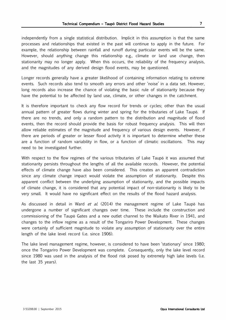
independently from a single statistical distribution. Implicit in this assumption is that the same
processes and relationships that existed in the past will continue to apply in the future. For
example, the relationship between rainfall and runoff during particular events will be the same.
However, should anything change this relationship e.g., climate or land use change, then
stationarity may no longer apply. When this occurs, the reliability of the frequency analysis,
and the magnitudes of any derived design flood events, may be questioned.
Longer records generally have a greater likelihood of containing information relating to extreme
events. Such records also tend to smooth any errors and other ‘noise’ in a data set. However,
long records also increase the chance of violating the basic rule of stationarity because they
have the potential to be affected by land use, climate, or other changes in the catchment.
It is therefore important to check any flow record for trends or cycles; other than the usual
annual pattern of greater flows during winter and spring for the tributaries of Lake Taupō. If
there are no trends, and only a random pattern to the distribution and magnitude of flood
events, then the record should provide the basis for robust frequency analysis. This will then
allow reliable estimates of the magnitude and frequency of various design events. However, if
there are periods of greater or lesser flood activity it is important to determine whether these
are a function of random variability in flow, or a function of climatic oscillations. This may
need to be investigated further.
With respect to the flow regimes of the various tributaries of Lake Taupō it was assumed that
stationarity persists throughout the lengths of all the available records. However, the potential
effects of climate change have also been considered. This creates an apparent contradiction
since any climate change impact would violate the assumption of stationarity. Despite this
apparent conflict between the underlying assumption of stationarity, and the possible impacts
of climate change, it is considered that any potential impact of non-stationarity is likely to be
very small. It would have no significant effect on the results of the flood hazard analysis.
As discussed in detail in Ward et al. (2014) the management regime of Lake Taupō has
undergone a number of significant changes over time. These include the construction and
commissioning of the Taupō Gates and a new outlet channel to the Waikato River in 1941, and
changes to the inflow regime as a result of the Tongariro Power Development. These changes
were certainly of sufficient magnitude to violate any assumption of stationarity over the entire
length of the lake level record (i.e. since 1906).
The lake level management regime, however, is considered to have been ‘stationary’ since 1980;
once the Tongariro Power Development was complete. Consequently, only the lake level record
since 1980 was used in the analysis of the flood risk posed by extremely high lake levels (i.e.
the last 35 years).

Technical Compendium Technical Compendium Technical Compendium Technical Compendium –––– TaupTaupTaupTaupō District Flood Hazard StudiesDistrict Flood Hazard StudiesDistrict Flood Hazard StudiesDistrict Flood Hazard Studies 8888
3-53208.00 | September 2015 Opus International Consultants LtdOpus International Consultants LtdOpus International Consultants LtdOpus International Consultants Ltd
Duration of flow record
The reliability of estimates of design lake levels and flood discharges is largely a function of
the length of flow record used in the analysis, and the appropriateness of the flow record to
a particular flood model.
As a general rule of thumb (Davie, 2008) average recurrence intervals (i.e. ARIs), or annual
exceedance probabilities (i.e. AEPs), should not be extrapolated beyond twice the length of the
record of annual flood maxima i.e. a 25-year flow series should only be used to estimate flood
events with an ARI of up to 50 years (i.e. 2%AEP). Uncertainty of flood estimates therefore
increases rapidly for more extreme events. Given the relatively short nature of the majority of
flow records used in the flood studies (Table 3.2), especially with respect to the magnitude of
the design flows of interest (i.e. 100-year ARI or 1%AEP), there will always be uncertainty over
the design flow estimates. This uncertainty can only be accommodated effectively by adopting
conservative, but still realistic values, and applying ‘best professional judgement’.
Table Table Table Table 3333....2222:::: Duration of Duration of Duration of Duration of the annual floodthe annual floodthe annual floodthe annual flood series used in series used in series used in series used in the the the the analysanalysanalysanalyseeees.s.s.s.
Hydrometric siteHydrometric siteHydrometric siteHydrometric site Duration of recordDuration of recordDuration of recordDuration of record
Lake Taupō ~35 years
Tongariro @ Turangi ~57 years
Tauranga Taupō @ Te Kono ~38 years
Kuratau @ SH41 ~36 years
Whareroa @ Fishtrap ~16 years
Hinemaiaia @ DS Dam ~28 years
Despite the uncertainty inherent in estimating the magnitudes of more extreme design flood
events, a sensitivity analysis of the various Taupō flood studies indicates that the extents and
depths of inundation are not extremely sensitive to the exact flood magnitude used in the
model. Any uncertainty in the design flood estimates is likely to have less effect on the result
than other uncertainties in the modelling as discussed later.
Alternative approaches
In situations where the flow record is extremely short (i.e. <20-years) and contains no large
flood events, an alternative method to a statistical analysis of the available flow record is
required. Possible methods for estimating design flows include: the regional method (McKerchar
and Pearson, 1989); translation and scaling of flows from adjacent and similar catchments; or
rainfall-runoff models. It should be noted that all these methods involve numerous assumptions;
the effects of which are usually difficult, and often impossible, to quantify. The uncertainty of
the outputs from these approaches is therefore generally significantly greater than that
associated with the analysis of specific flow records.
The flow data which currently underpin the regional method outlined in McKerchar and Pearson
(1989) ends in 1985. Consequently there are approximately 30-years of additional site specific
data now available for the major tributaries into Lake Taupō. These data add significantly more

Technical Compendium Technical Compendium Technical Compendium Technical Compendium –––– TaupTaupTaupTaupō District Flood Hazard StudiesDistrict Flood Hazard StudiesDistrict Flood Hazard StudiesDistrict Flood Hazard Studies 9999
3-53208.00 | September 2015 Opus International Consultants LtdOpus International Consultants LtdOpus International Consultants LtdOpus International Consultants Ltd
to the robustness of estimates of the magnitudes of various design events in these specific
rivers than generalised indices based on the shorter, less accurate flow series used in McKerchar
and Pearson (1989). In addition, the annual flood maxima from a number of the major
tributaries to Lake Taupō were used in McKerchar and Pearson (1989); for example, Tongariro
@ Turangi, Tauranga Taupō @ Te Kono, and Wanganui @ Te Porere (which does not flow into
Lake Taupō). To use the regional method for these rivers would appear to introduce some
circularity and bias to any analysis.
The regional flood frequency indices are currently being revised and updated to include all
information collected since the original report (i.e. since 1985). Once these new indices are
available they are likely to add significantly to the robustness and consistency of flood frequency
analyses obtained from short flow series. However, at this stage it is considered that the
additional 35 years of data available for the specific rivers and streams modelled in the Taupō
flood study adds more to the robustness of design flood estimates than potentially ‘smoothing’
the data through the use of generalised indices from McKerchar and Pearson (1989).
The reliability of rainfall-runoff models is largely determined by the quality of the calibration
and validation. It also depends on the nature of the rainfall-runoff relationship within the
catchment, and how this is ‘captured’ by the calibration and validation. Since calibration and
validation are invariably undertaken on flows significantly less than the required design discharge
(i.e. the 1%AEP flood), the nature of this relationship, and how it changes with flood magnitude,
is critical. Consequently, the assumptions relating to rainfall distribution across the catchment,
and the simplifications required within a rainfall-runoff model usually result in greater uncertainty
than is likely from the use of even relatively short duration flow records.
These alternative methodologies, however, can be valuable in providing an ‘independent’ check
on the likely reliability of design flood estimates from short flow records e.g., Whareroa @
Fishtrap and Tokaanu Stream.
3.33.33.33.3 Flow seriesFlow seriesFlow seriesFlow series
Each flow series for the rivers flowing into Lake Taupō was reviewed to assess the quality of
the flow record, including: any gaps in the record; the accuracy and appropriateness of the
rating curves for estimating discharge at higher flows; the annual maxima flood series; and the
frequency analysis used to derive estimates of the magnitudes of the design flood events.
Tongariro River
The longest and most suitable flow series to assess the flood risk to Turangi is from the
Tongariro River at Turangi site; operated and maintained by NIWA. A discussion of this flow
record is available in Maas & McConchie (2011). To supplement that discussion, further analysis
of the quality of the flow record is provided.
The flow record provided by NIWA shows no gaps (i.e. missing data) between 1957 and 2014.
The comment file for this site, however, indicates that there was initially one gap during January

Technical Compendium Technical Compendium Technical Compendium Technical Compendium –––– TaupTaupTaupTaupō District Flood Hazard StudiesDistrict Flood Hazard StudiesDistrict Flood Hazard StudiesDistrict Flood Hazard Studies 10101010
3-53208.00 | September 2015 Opus International Consultants LtdOpus International Consultants LtdOpus International Consultants LtdOpus International Consultants Ltd
2007; of approximately eight hours. That gap was ‘filled’ after comparing flows with those
recorded at a site located further upstream.
The rating curves for the Tongariro at Turangi flow site are shown in Figure 3.1. There have
been 58 ratings used between 1957 and 2012. The gaugings used to define the various rating
curves are also plotted in Figure 3.1. The highest gauged flow was on 24 February 1958 at
1470m³/s. This is also the largest flow on record. Given the historic nature of this flood,
there is some uncertainty as to whether the flood was actually gauged at its peak. Also, given
the extreme nature of this event there is some uncertainty over the accuracy of the gauging.
However, this is the information within the ‘comment file’ and therefore it has been assumed to
be correct. There is no basis currently to disregard this information.
An analysis of the stage data during the second largest flood on record (i.e., that of 29 February
2004) shows apparently large variations in the bed level over short periods of time (Figure 3.2).
This bed instability affects the estimated flood flows and also impacts on the accuracy of any
hydraulic model. The hydrological and hydraulic controls which cause this bed instability are
inherent in the dynamics of flood events. Such channel instability cannot be modelled and
therefore the uncertainty caused by this variability can only be incorporated through conservative
design assumptions.
Figure Figure Figure Figure 3333....1111:::: Rating curves for Rating curves for Rating curves for Rating curves for the the the the Tongariro Tongariro Tongariro Tongariro River River River River at Turangiat Turangiat Turangiat Turangi....
0 100 200 300 400 500 600 700 800 900 1000 1100 1200 1300 14001500
0
500
1000
1500
2000
2500
3000
3500
4000
4500
Flow (m³/sec)
Tongariro at Turangi from 1-Jan-1957 00:00:00 to 16-Jul-2012 11:00:00 0%% error bars
Sta
ge
(m
m)

Technical Compendium Technical Compendium Technical Compendium Technical Compendium –––– TaupTaupTaupTaupō District Flood Hazard StudiesDistrict Flood Hazard StudiesDistrict Flood Hazard StudiesDistrict Flood Hazard Studies 11111111
3-53208.00 | September 2015 Opus International Consultants LtdOpus International Consultants LtdOpus International Consultants LtdOpus International Consultants Ltd
Figure Figure Figure Figure 3333....2222:::: Stage and flow readings for 29 Feb 2004 flood Stage and flow readings for 29 Feb 2004 flood Stage and flow readings for 29 Feb 2004 flood Stage and flow readings for 29 Feb 2004 flood in thein thein thein the Tongariro Tongariro Tongariro Tongariro River River River River at Turangiat Turangiat Turangiat Turangi....
Despite these various sources of uncertainty, it has been assumed that the instrumental flow
series has been collected using ‘industry best practice’. While there will also be uncertainty as
to the exact magnitude of flood flows, those represented in the Tongariro at Turangi record
are considered robust, and are certainly the best available for any flood hazard analysis.
The annual maxima flood series for Tongariro at Turangi is shown in Figure 3.3. There is no
obvious longer term trend in the data, and the magnitude and distribution of flood events
appear essentially random. There appears, however, to be some indication of minor cyclic
behaviour and persistence; with periods of generally larger floods interspersed with periods of
smaller annual events.
Figure Figure Figure Figure 3333....3333:::: Annual maxima flood series for Tongariro Annual maxima flood series for Tongariro Annual maxima flood series for Tongariro Annual maxima flood series for Tongariro River River River River at Turangi (1957at Turangi (1957at Turangi (1957at Turangi (1957----2014)2014)2014)2014)....
Implicit in the frequency analysis of annual flood maxima series is that the events are
independent, drawn from a single distribution, and that stationarity has persisted throughout
12:00:00 18:00:00 29-Feb-2004 06:00:00 12:00:00 18:00:00
2000
2200
2400
2600
2800
3000
3200
3400
3600
3800
4000
4200
4400
4600
0
115
231
346
462
577
692
808
923
1038
1154
1269
1385
1500
Sta
ge (
mm
)
Flo
w (
m³/
sec)
Tongariro at Turangi Stage (mm)Tongariro at Turangi Flow (m³/sec)
0
200
400
600
800
1000
1200
1400
1600
Annual Maximum Flow (m³/s)

Technical Compendium Technical Compendium Technical Compendium Technical Compendium –––– TaupTaupTaupTaupō District Flood Hazard StudiesDistrict Flood Hazard StudiesDistrict Flood Hazard StudiesDistrict Flood Hazard Studies 12121212
3-53208.00 | September 2015 Opus International Consultants LtdOpus International Consultants LtdOpus International Consultants LtdOpus International Consultants Ltd
the length of record. It would appear from Figure 3.3 that this is the case with respect to the
record from the Tongariro River at Turangi. To ensure that all events in the flood series are
independent, the flow series was reviewed. All the flood maxima are separated from other large
events in the series by a considerable period of time indicating that all the flood maxima are
independent events. The effect of any departure from the basic assumptions is therefore likely
to be very small relative to the uncertainty inherent in; firstly, the magnitudes of the events in
the annual maxima series, and then the magnitude and frequency of any design events.
It is problematic that if the assumption of stationarity is not valid then any robust frequency
analysis would not be possible.
An updated frequency analysis of the Tongariro at Turangi record has been undertaken using
the extended record up until the end of 2014. This included an analysis of the L moments
(Figure 3.4) and the appropriateness of various statistical distributions when modelling the annual
flood maxima series (Figure 3.5).
The L moment analysis indicates that a GEV or Generalised Logistic statistical distribution would
best represent the Tongariro at Turangi flow series. However, when analysing these distributions
on the frequency analysis plot, both appear to have an unrealistic shape. The GEV, Generalised
Logistic and Log Normal distribution all increase ‘exponentially’ with increasing ARI or decreasing
AEP (Figure 3.5). The statistical distribution with the most realistic and ‘natural’ shape is that
provided by the PE3 distribution.
Figure Figure Figure Figure 3333....4444:::: L momentL momentL momentL moment analysis for analysis for analysis for analysis for the the the the Tongariro at Tongariro at Tongariro at Tongariro at TurangiTurangiTurangiTurangi annual flood maxima series.annual flood maxima series.annual flood maxima series.annual flood maxima series.
-0.2 -0.1 0.0 0.1 0.2 0.3 0.4 0.5 0.6 0.7
-0.1
0.0
0.1
0.2
0.3
0.4
0.5
Gumbel
GEV
Generalised Logistic
Generalised Pareto
Log Normal
Pearson Type 3
L-Moment Ratios: L-Kurtosis versus L-SkewnessFlow (m³/sec) at Tongariro at Turangi from 1-Jan-1957 06:00 to 1-Oct-2014 00:00

Technical Compendium Technical Compendium Technical Compendium Technical Compendium –––– TaupTaupTaupTaupō District Flood Hazard StudiesDistrict Flood Hazard StudiesDistrict Flood Hazard StudiesDistrict Flood Hazard Studies 13131313
3-53208.00 | September 2015 Opus International Consultants LtdOpus International Consultants LtdOpus International Consultants LtdOpus International Consultants Ltd
Figure Figure Figure Figure 3333....5555:::: Frequency analysis for Tongariro at TurangiFrequency analysis for Tongariro at TurangiFrequency analysis for Tongariro at TurangiFrequency analysis for Tongariro at Turangi annual flood maxima series.annual flood maxima series.annual flood maxima series.annual flood maxima series.
Estimates of various design flood events, assuming several different statistical distributions, are
listed in Table 3.3. The PE3 results are highlighted and are considered the more realistic. It
should be noted that the difference between the magnitude of the 100-year flood event (i.e.
1%AEP) assuming a PE3 distribution is 164m³/s lower than the highest estimate, and 153m³/s
higher than the lowest estimate i.e. the difference is only ±11% of the estimated peak discharge.
Given the uncertainties inherent in estimating the magnitudes of various design flood events,
these differences are not significant. They would have no effect on the outcome of any flood
hazard analysis.
Table Table Table Table 3333....3333:::: Results of frequency analysis for Tongariro at TurangiResults of frequency analysis for Tongariro at TurangiResults of frequency analysis for Tongariro at TurangiResults of frequency analysis for Tongariro at Turangi 1957195719571957----2014 (m³/s)2014 (m³/s)2014 (m³/s)2014 (m³/s)....
ARIARIARIARI GEVGEVGEVGEV GeneralisedGeneralisedGeneralisedGeneralised
LogisticLogisticLogisticLogistic
GeneralisedGeneralisedGeneralisedGeneralised
ParetoParetoParetoPareto
LogLogLogLog
NormalNormalNormalNormal PE3PE3PE3PE3 GumbelGumbelGumbelGumbel
2.332.332.332.33 428 431 426 442 427 462
5555 609 598 640 625 634 645
10101010 783 763 824 785 817 794
20202020 976 956 1002 949 998 937
50505050 1272 1274 1225 1173 1235 1121
100100100100 1533 1577 1385 1351 1413 1260
Despite some inherent uncertainty in estimates of the magnitude of flood flows, those derived
for the Tongariro River at Turangi are considered robust. They are the best available for any
flood hazard analysis and hydraulic modelling.
1.0 0.5 0.2 0.1 0.05 0.02 0.01 0.005 0.002 0.001 0.0005 0.0002
0
200
400
600
800
1000
1200
1400
1600
1800
2000
FEDCBAzyxwvuts
rqponmlkjih
gfedcbaZYXWVUT
SRQPO
NMLKJ I
H GF E
D
C
B A
A-F Flow (m³/sec) at Tongariro at Turangi From 1-Jan-1957 06:00:00 to 1-Oct-2014 00:00:00 GEV Distribution: Location = 332 Scale = 158 Shape = -0.202 GenLog Distribution: Location = 396 Scale = 117 Shape = -0.307 GenPareto Distribution: Location = 179 Scale = 301 Shape = 0.0611 Normal Distribution: Mean = 6.01 Std.Dev = 0.915 Pearson3 Distribution: Location = 462 Scale = 270 Shape = 1.84 Gumbel Distribution: Location = 348 Scale = 198

Technical Compendium Technical Compendium Technical Compendium Technical Compendium –––– TaupTaupTaupTaupō District Flood Hazard StudiesDistrict Flood Hazard StudiesDistrict Flood Hazard StudiesDistrict Flood Hazard Studies 14141414
3-53208.00 | September 2015 Opus International Consultants LtdOpus International Consultants LtdOpus International Consultants LtdOpus International Consultants Ltd
Tauranga Taupō River
The longest and most suitable flow series to assess the flood risk posed by the Tauranga
Taupō River is from Te Kono; a site operated and maintained by Waikato Regional Council. A
discussion of this flow record is available in Knight (2010). To supplement that discussion,
further analysis of the quality of the flow record is provided.
The flow record provided by Waikato Regional Council shows 35 gaps between 1976 and 2014.
These gaps span a total of 7372 hours (i.e. 307 days). The majority of these gaps (i.e. 80%)
are less than a week long (Table 3.4); however, 80% of time total time represented by the gaps
is the result of longer duration periods of missing record (i.e. >1 week duration).
Table Table Table Table 3333....4444:::: Gap analysis of TaurangaGap analysis of TaurangaGap analysis of TaurangaGap analysis of Tauranga TaupTaupTaupTaupō at Te Kono flow recordat Te Kono flow recordat Te Kono flow recordat Te Kono flow record....
DurationDurationDurationDuration Number of gapsNumber of gapsNumber of gapsNumber of gaps Total hoursTotal hoursTotal hoursTotal hours
>1 week 7 5922
<1 week 15 1315
< 1day 13 135
The rating curves for the Tauranga Taupō at Te Kono flow site are shown in Figure 3.6; together
with the gaugings used to define the various curves. All these data were provided by Waikato
Regional Council.
There were 250 flow gaugings between 1981 and 2015. The highest gauged flow was on 12
July 2008 at 151m³/s, while the largest flow on record is 296m³/s. Consequently the highest
gauged flow is only about half the estimated magnitude of the largest flood event. This results
in some uncertainty regarding the estimated peak discharges of larger flood events.
Figure Figure Figure Figure 3333....6666:::: Rating curves for the Rating curves for the Rating curves for the Rating curves for the TaurangaTaurangaTaurangaTauranga TaupTaupTaupTaupō RiverRiverRiverRiver at Te Konoat Te Konoat Te Konoat Te Kono....

Technical Compendium Technical Compendium Technical Compendium Technical Compendium –––– TaupTaupTaupTaupō District Flood Hazard StudiesDistrict Flood Hazard StudiesDistrict Flood Hazard StudiesDistrict Flood Hazard Studies 15151515
3-53208.00 | September 2015 Opus International Consultants LtdOpus International Consultants LtdOpus International Consultants LtdOpus International Consultants Ltd
The annual flood maxima series for the Tauranga Taupō River at Te Kono is shown in Figure
3.7. There is no obvious longer term trend in the data, and the magnitude and distribution of
the flood events appear essentially random. There appears, however, to be some indication of
minor cyclic behaviour and persistence; with periods of generally larger floods interspersed with
periods of smaller annual events.
Implicit in any frequency analysis of annual flood maxima series is that the events are
independent, drawn from a single distribution, and that stationarity has persisted throughout
the length of record. It would appear from Figure 3.7 that this is the case with respect to the
flow record from the Tauranga Taupō River at Te Kono. To ensure that all events in the flood
series are independent, the flow series was reviewed. All the flood maxima are separated from
other large events in the series by a considerable period of time indicating that all the flood
maxima are independent events. The effect of any departure from these assumptions is
therefore likely to be very small relative to the uncertainty inherent in; firstly, the magnitudes
of the events in the annual maxima series, and then the estimated magnitude and frequency
of any design events.
It is problematic that if the assumption of stationarity is not valid then any robust frequency
analysis would not be possible.
Figure Figure Figure Figure 3333....7777:::: Annual maxima flood series for Annual maxima flood series for Annual maxima flood series for Annual maxima flood series for TaurangaTaurangaTaurangaTauranga TaupTaupTaupTaupō RiverRiverRiverRiver at Te Konoat Te Konoat Te Konoat Te Kono (19(19(19(1976767676----2014201420142014).).).).
An updated frequency analysis of the Tauranga Taupō River at Te Kono flow record has been
undertaken using the extended record up until the end of 2014. This included an analysis of
the L moments (Figure 3.8) and the appropriateness of assuming various statistical distributions
when analysing the annual flood maxima series (Figure 3.9).
0
50
100
150
200
250
300
350
1976
1977
1978
1979
1980
1981
1982
1983
1984
1985
1986
1987
1988
1989
1990
1991
1992
1993
1994
1995
1996
1997
1998
1999
2000
2001
2002
2003
2004
2005
2006
2007
2008
2009
2010
2011
2012
2013
2014
Annual Maximum Flow (m³/s)

Technical Compendium Technical Compendium Technical Compendium Technical Compendium –––– TaupTaupTaupTaupō District Flood Hazard StudiesDistrict Flood Hazard StudiesDistrict Flood Hazard StudiesDistrict Flood Hazard Studies 16161616
3-53208.00 | September 2015 Opus International Consultants LtdOpus International Consultants LtdOpus International Consultants LtdOpus International Consultants Ltd
Figure Figure Figure Figure 3333....8888:::: L momentL momentL momentL moment analysis for analysis for analysis for analysis for TaurangaTaurangaTaurangaTauranga TaupTaupTaupTaupō River at Te KonoRiver at Te KonoRiver at Te KonoRiver at Te Kono annual flood maxima seriesannual flood maxima seriesannual flood maxima seriesannual flood maxima series....
The L moment analysis indicates that a PE3 distribution best represents the annual flood maxima
series for the Tauranga Taupō River at Te Kono; although a GEV distribution gives almost the
same design flows. When analysing the various statistical distributions, the PE3 statistical
distribution appears to have both a realistic shape and plots closest to the largest floods.
Figure Figure Figure Figure 3333....9999:::: Frequency analysis for Frequency analysis for Frequency analysis for Frequency analysis for TaurangaTaurangaTaurangaTauranga TaupTaupTaupTaupō River at Te KonoRiver at Te KonoRiver at Te KonoRiver at Te Kono annual flood maxima seriesannual flood maxima seriesannual flood maxima seriesannual flood maxima series....
The results assuming several different statistical distributions are listed in Table 3.5. The PE3
results are highlighted and are considered the most reliable. It should be noted that the
-0.2 -0.1 0.0 0.1 0.2 0.3 0.4 0.5 0.6 0.7
-0.1
0.0
0.1
0.2
0.3
0.4
0.5
Gumbel
GEV
Generalised Logistic
Generalised Pareto
Log Normal
Pearson Type 3
L-Moment Ratios: L-Kurtosis versus L-SkewnessFlow (m³/s) at Tauranga-Taupo at Te Kono Road from 11-Feb-1976 14:15 to 20-Jan-2015 13:45
1.0 0.5 0.2 0.1 0.05 0.02 0.01 0.005 0.002 0.001 0.0005 0.0002
0
50
100
150
200
250
300
350
400
450
500
lkjihgfe
dcbaZYX
WVUT
SRQPON
MLKJ I H G F E
D
C B
A
A-l Flow (m³/s) at Tauranga-Taupo at Te Kono From 11-Feb-1976 14:15:00 to 31-Dec-2013 23:55:00 GEV Distribution: Location = 121 Scale = 51.6 Shape = 0.0619 GenLog Distribution: Location = 140 Scale = 33 Shape = -0.131 GenPareto Distribution: Location = 61.6 Scale = 132 Shape = 0.538 Normal Distribution: Mean = 4.91 Std.Dev = 0.756 Pearson3 Distribution: Location = 148 Scale = 61.3 Shape = 0.797 Gumbel Distribution: Location = 119 Scale = 48.9

Technical Compendium Technical Compendium Technical Compendium Technical Compendium –––– TaupTaupTaupTaupō District Flood Hazard StudiesDistrict Flood Hazard StudiesDistrict Flood Hazard StudiesDistrict Flood Hazard Studies 17171717
3-53208.00 | September 2015 Opus International Consultants LtdOpus International Consultants LtdOpus International Consultants LtdOpus International Consultants Ltd
difference between the magnitude of the 100-year flood event assuming a PE3 statistical
distribution is only 23m³/s lower than the highest estimate, and only 38m³/s higher than the
lowest estimate i.e. the difference is only about ±10% of the estimated peak discharge during
the 100-year ARI event. Given the uncertainties inherent in estimating the magnitudes of various
design flood events, these differences are not significant. They would have no effect on the
outcome of any flood hazard analysis.
Table Table Table Table 3333....5555:::: Results of frequency analysis for Results of frequency analysis for Results of frequency analysis for Results of frequency analysis for TaurangaTaurangaTaurangaTauranga TaupTaupTaupTaupō at Te Kono at Te Kono at Te Kono at Te Kono 1976197619761976----2015201520152015 (m³/s)(m³/s)(m³/s)(m³/s)....
ARIARIARIARI GEVGEVGEVGEV GeneralisedGeneralisedGeneralisedGeneralised
LogisticLogisticLogisticLogistic
GeneralisedGeneralisedGeneralisedGeneralised
ParetoParetoParetoPareto
LogLogLogLog
NormalNormalNormalNormal PE3PE3PE3PE3 GumbelGumbelGumbelGumbel
2.332.332.332.33 147 147 149 141 148 144
5555 193 188 203 193 193 190
10101010 227 222 234 238 227 228
20202020 258 256 255 282 258 264
50505050 295 304 272 342 294 311
100100100100 321 343 280 389 320 346
Despite some inherent uncertainty in the estimates of the magnitude of flood flows, those
derived for the Tauranga Taupō at Te Kono record are considered robust. They are the best
available for any flood hazard analysis and hydraulic modelling.
Hinemaiaia River
The longest and most suitable flow series to assess the flood risk posed by the Hinemaiaia
River is from a site operated and maintained for TrustPower by NIWA. A discussion of this flow
record from the Hinemaiaia “Below HB dam” is available in Paine & Smith (2012a). To
supplement that discussion, further analysis of the quality of the flow record is provided.
The flow record provided by NIWA for this site shows six gaps between 2000 and 2014. These
gaps span a total of 349 hours (i.e. 15 days). One gap lasts for less than a day while the
others are up to a week duration (Table 3.4). Gaps of between one day and one week make
up 94% of the total period of missing data.
Table Table Table Table 3333....6666:::: Gap analysis of Gap analysis of Gap analysis of Gap analysis of Hinemaiaia River at Below HB Dam Hinemaiaia River at Below HB Dam Hinemaiaia River at Below HB Dam Hinemaiaia River at Below HB Dam flow recordflow recordflow recordflow record....
DurationDurationDurationDuration Number of gapsNumber of gapsNumber of gapsNumber of gaps Total hoursTotal hoursTotal hoursTotal hours
>1 week 0 0
<1 week 5 327
< 1day 1 22
The rating curves for the Hinemaiaia River at Below HB Dam flow site are shown in Figure 3.10.
Eight different ratings were used between 2000 and 2013. The gaugings used to define the
various rating curves are also plotted in Figure 3.10.

Technical Compendium Technical Compendium Technical Compendium Technical Compendium –––– TaupTaupTaupTaupō District Flood Hazard StudiesDistrict Flood Hazard StudiesDistrict Flood Hazard StudiesDistrict Flood Hazard Studies 18181818
3-53208.00 | September 2015 Opus International Consultants LtdOpus International Consultants LtdOpus International Consultants LtdOpus International Consultants Ltd
Figure Figure Figure Figure 3333....10101010:::: Rating curves for the Rating curves for the Rating curves for the Rating curves for the Hinemaiaia River at Below HB DamHinemaiaia River at Below HB DamHinemaiaia River at Below HB DamHinemaiaia River at Below HB Dam....
The highest gauged flow was on 24 July 2000 at 8.433m³/s, while the largest flow on record
is estimated at 87.5m³/s. Consequently the highest gauged flow is only about 10% of the
largest estimated flow. This is likely to result in some uncertainty regarding the estimated peak
discharges of larger flood events. Despite this, as discussed in Paine and Smith (2011), the
Hinemaiaia at Below HB Dam flow record, augmented with earlier flows measured at an adjacent
site, provides the most suitable annual flood maxima series for use when assessing the flood
risk posed by the Hinemaiaia River.
The annual flood maxima series for Hinemaiaia River at Below HB Dam is shown in Figure 3.11.
There is no obvious longer term trend in the data, and the magnitude and distribution of flood
events appear essentially random. The flow record at this site is relatively short and therefore
any pattern is difficult to determine. However, the extended annual flood maxima series
discussed in Paine & Smith (2012a) also shows no longer term trend in either flood frequency
or magnitude.
Implicit in the frequency analysis of an annual flood maxima series is that the events are
independent, drawn from a single distribution, and that stationarity has persisted throughout
the length of record. It would appear from Figure 3.11, and the detailed discussion provided
in Paine & Smith (2012a), that this is the case with respect to the flow record from the
Hinemaiaia River. To ensure that all events in the flood series are independent, the flow series
was reviewed. All the flood maxima are separated from other large events in the series by a
considerable period of time. This indicates that all the flood maxima are independent events.
The effect of any departure from these assumptions is therefore likely to be very small relative
0 10 20 30 40 50 60 70 80 90 100
0
200
400
600
800
1000
1200
1400
1600
1800
2000
2200
2400
2600
Flow (m³/sec)
Hinemaiaia at Below HB Dam from 19-Jun-2000 12:00:00 to 21-Jul-2014 15:30:00 0%% error bars
Sta
ge (
mm
)

Technical Compendium Technical Compendium Technical Compendium Technical Compendium –––– TaupTaupTaupTaupō District Flood Hazard StudiesDistrict Flood Hazard StudiesDistrict Flood Hazard StudiesDistrict Flood Hazard Studies 19191919
3-53208.00 | September 2015 Opus International Consultants LtdOpus International Consultants LtdOpus International Consultants LtdOpus International Consultants Ltd
to the uncertainty inherent in; firstly, the magnitudes of the events in the annual maxima series,
and then the estimated magnitude and frequency of any design events.
Figure Figure Figure Figure 3333....11111111:::: Annual maxima flood series for Annual maxima flood series for Annual maxima flood series for Annual maxima flood series for Hinemaiaia River at Below HB Dam Hinemaiaia River at Below HB Dam Hinemaiaia River at Below HB Dam Hinemaiaia River at Below HB Dam ((((2000200020002000----2014201420142014).).).).
An updated frequency analysis of the Hinemaiaia River at Below HB Dam record from 2000-
2014 was undertaken. This included an analysis of the L moments (Figure 3.12) and the
appropriateness of assuming various statistical distributions when analysing the annual flood
maxima series (Figure 3.13).
Figure Figure Figure Figure 3333....12121212:::: L moment analysis for L moment analysis for L moment analysis for L moment analysis for Hinemaiaia River at Below HB DamHinemaiaia River at Below HB DamHinemaiaia River at Below HB DamHinemaiaia River at Below HB Dam annual flood maxima seriesannual flood maxima seriesannual flood maxima seriesannual flood maxima series....
0
10
20
30
40
50
60
70
80
90
2001 2002 2003 2004 2005 2006 2007 2008 2009 2010 2011 2012 2013 2014
Annual Maximum Flow (m³/s)
-0.2 -0.1 0.0 0.1 0.2 0.3 0.4 0.5 0.6 0.7
-0.1
0.0
0.1
0.2
0.3
0.4
0.5
Gumbel
GEV
Generalised Logistic
Generalised Pareto
Log Normal
Pearson Type 3
L-Moment Ratios: L-Kurtosis versus L-SkewnessFlow (m³/sec) at Hinemaiaia at Below HB Dam from 19-Jun-2000 12:00 to 1-Oct-2014 00:00

Technical Compendium Technical Compendium Technical Compendium Technical Compendium –––– TaupTaupTaupTaupō District Flood Hazard StudiesDistrict Flood Hazard StudiesDistrict Flood Hazard StudiesDistrict Flood Hazard Studies 20202020
3-53208.00 | September 2015 Opus International Consultants LtdOpus International Consultants LtdOpus International Consultants LtdOpus International Consultants Ltd
Figure Figure Figure Figure 3333....13131313:::: Frequency analFrequency analFrequency analFrequency analysis for ysis for ysis for ysis for Hinemaiaia River at Below HB DamHinemaiaia River at Below HB DamHinemaiaia River at Below HB DamHinemaiaia River at Below HB Dam annual flood maxima seriesannual flood maxima seriesannual flood maxima seriesannual flood maxima series....
The L moment analysis indicates that a Generalised Pareto distribution best represents the
annual flood maxima series for the Hinemaiaia River at Below HB Dam; although both the PE3
and Gumbel statistical distributions also provide almost identical design flows. When reviewing
these distributions on the frequency analysis plot (Figure 3.13), the Generalised Pareto statistical
distribution appears to flatten off significantly at higher flows when compared with the other
distributions. Such a characteristic appears atypical of accepted flood behaviour in New Zealand.
The most realistic statistical distribution is therefore considered to be either the PE3 or Gumbel.
The adoption of the PE3 statistical distribution is slightly conservative. It results in a slightly
higher estimate of the magnitude of the 1%AEP design flood event.
The results assuming several different statistical distributions are listed in Table 3.7. The PE3
results are highlighted and are considered the more reliable. It should be noted that the
difference between the magnitude of the 1%AEP design flood event using the PE3 statistical
distribution is only 19m³/s lower than the highest estimate, and only 7m³/s higher than the
lowest estimate i.e. the difference is only from 6-15% of the estimated peak discharge during
the design event. Given the uncertainties inherent in estimating the magnitudes of various
design flood events, these differences are not significant. They would have no effect on the
outcome of any flood hazard analysis.
1.0 0.5 0.2 0.1 0.05 0.02 0.01 0.005 0.002 0.001 0.0005 0.0002
0
20
40
60
80
100
120
140
160
180
200
ONMLKJ
I H G FE
DC
B A
A-O Flow (m³/sec) at Hinemaiaia at Below HB Dam From 19-Jun-2000 12:00:00 to 1-Oct-2014 00:00:00 GEV Distribution: Location = 26.6 Scale = 16.6 Shape = -0.135 GenLog Distribution: Location = 33.3 Scale = 11.8 Shape = -0.26 GenPareto Distribution: Location = 9.94 Scale = 33.9 Shape = 0.175 Normal Distribution: Mean = 3.48 Std.Dev = 1.13 Pearson3 Distribution: Location = 38.8 Scale = 25.3 Shape = 1.56 Gumbel Distribution: Location = 27.7 Scale = 19.1

Technical Compendium Technical Compendium Technical Compendium Technical Compendium –––– TaupTaupTaupTaupō District Flood Hazard StudiesDistrict Flood Hazard StudiesDistrict Flood Hazard StudiesDistrict Flood Hazard Studies 21212121
3-53208.00 | September 2015 Opus International Consultants LtdOpus International Consultants LtdOpus International Consultants LtdOpus International Consultants Ltd
Table Table Table Table 3333....7777:::: Results of frequency analysis for Results of frequency analysis for Results of frequency analysis for Results of frequency analysis for Hinemaiaia at Below HB Dam Hinemaiaia at Below HB Dam Hinemaiaia at Below HB Dam Hinemaiaia at Below HB Dam 2000200020002000----2014 (m³/s)2014 (m³/s)2014 (m³/s)2014 (m³/s)....
ARIARIARIARI GEVGEVGEVGEV GeneralisedGeneralisedGeneralisedGeneralised
LogisticLogisticLogisticLogistic
GeneralisedGeneralisedGeneralisedGeneralised
ParetoParetoParetoPareto
LogLogLogLog
NormalNormalNormalNormal PE3PE3PE3PE3 GumbelGumbelGumbelGumbel
2.332.332.332.33 37 37 37 36 37 39
5555 54 53 57 56 56 56
10101010 70 68 74 74 72 71
20202020 87 86 89 93 88 85
50505050 112 113 106 120 109 102
100100100100 133 138 117 143 124 116
Despite some uncertainty inherent in the estimates of the magnitude of flood flows, those
derived for the Hinemaiaia River using all available flow data are considered robust. They are
the best available for any flood hazard analysis and hydraulic modelling.
Tokaanu Stream
There have been two flow sites on the Tokaanu Stream downstream of the power station tail
race. However, both sites were closed after only a relatively short period of time (i.e. 22 and
60 months respectively).
Following discussions with the local NIWA Field Team, who have an extensive understanding of
the hydrology of the wider area, it was decided that the most realistic flood frequency estimates
would be obtained by scaling results from the adjacent Whanganui at Te Porere flow site. The
appropriateness and limitations of this approach are discussed in Paine & Smith (2012b). To
supplement that discussion, further analysis of the quality of the flow record from Whanganui
at Te Porere is provided.
The flow record provided by NIWA for the Whanganui at Te Porere flow site between 1966 and
2014 shows one gap. The period of missing record lasts only 1.26 days. This gap therefore
represents 0.007% of the total length of record and is likely to be inconsequential.
The rating curves for the Whanganui at Te Porere flow site are shown in Figure 3.14; together
with the gaugings used to define the various curves. There have been 37 different ratings used
between 1966 and 2014. The highest gauged flow was on 9 March 1990 at 51.8m³/s, while
the largest estimated flow on record is 54.0m³/s. Therefore the highest gauged flow is
approximately 96% of the largest estimated flow. This allows a high level of confidence to be
placed in the estimates of larger flood events, and consequently the annual flood maxima
series.
The annual flood maxima series for Whanganui at Te Porere is shown in Figure 3.15. There is
no obvious longer term trend in the data, and the magnitude and distribution of the flood
events appear essentially random. There appears, however, to be some indication of minor
cyclic behaviour or persistence; with periods of generally larger floods interspersed with periods
of smaller annual events.

Technical Compendium Technical Compendium Technical Compendium Technical Compendium –––– TaupTaupTaupTaupō District Flood Hazard StudiesDistrict Flood Hazard StudiesDistrict Flood Hazard StudiesDistrict Flood Hazard Studies 22222222
3-53208.00 | September 2015 Opus International Consultants LtdOpus International Consultants LtdOpus International Consultants LtdOpus International Consultants Ltd
Figure Figure Figure Figure 3333....14141414:::: Rating curves for the Rating curves for the Rating curves for the Rating curves for the Whanganui at Te PorereWhanganui at Te PorereWhanganui at Te PorereWhanganui at Te Porere....
Figure Figure Figure Figure 3333....15151515:::: Annual maxima flood series for Annual maxima flood series for Annual maxima flood series for Annual maxima flood series for Whanganui at Te PorereWhanganui at Te PorereWhanganui at Te PorereWhanganui at Te Porere ((((1966196619661966----2014).2014).2014).2014).
Implicit in any frequency analysis of an annual flood maxima series is that the events are
independent, drawn from a single distribution, and that stationarity has persisted throughout
the length of record. It would appear from Figure 3.15 that this is the case with respect to
the flow record from the Whanganui at Te Porere. To ensure that all events in the flood series
are independent, the flow series was reviewed. All the flood maxima are separated from other
large events in the series by a considerable period of time. This indicates that all the flood
maxima are independent events. The effect of any departure from these assumptions are likely
to be very small relative to the uncertainty inherent in; firstly, the magnitudes of the events in
0 5 10 15 20 25 30 35 40 45 50 55 60
0
200
400
600
800
1000
1200
1400
1600
1800
2000
2200
2400
Flow (m³/sec)
Whanganui R at Te Porere from 13-Jan-1966 00:00:00 to 3-Sep-2014 10:50:00 0%% error bars
Sta
ge (
mm
)
0
10
20
30
40
50
60
1966 1968 1970 1972 1974 1976 1978 1980 1982 1984 1986 1988 1990 1992 1994 1996 1998 2000 2002 2004 2006 2008 2010 2012 2014
Annual Maximum Flow (m³/s)

Technical Compendium Technical Compendium Technical Compendium Technical Compendium –––– TaupTaupTaupTaupō District Flood Hazard StudiesDistrict Flood Hazard StudiesDistrict Flood Hazard StudiesDistrict Flood Hazard Studies 23232323
3-53208.00 | September 2015 Opus International Consultants LtdOpus International Consultants LtdOpus International Consultants LtdOpus International Consultants Ltd
the annual maxima series, and then the magnitude and frequency of any design events. It is
problematic that if the assumption of stationarity is not valid then any robust frequency analysis
would not be possible.
An updated frequency analysis of the Whanganui at Te Porere annual flood maxima series was
undertaken using the extended record up until the end of 2014. This included an analysis of
the L moments (Figure 3.16) and various frequency distributions (Figure 3.17).
Figure Figure Figure Figure 3333....16161616:::: L moment analysis for L moment analysis for L moment analysis for L moment analysis for Whanganui at Te PorereWhanganui at Te PorereWhanganui at Te PorereWhanganui at Te Porere annual flood maxima seriesannual flood maxima seriesannual flood maxima seriesannual flood maxima series....
Figure Figure Figure Figure 3333....17171717:::: Frequency analysis for Frequency analysis for Frequency analysis for Frequency analysis for Whanganui at Te PorereWhanganui at Te PorereWhanganui at Te PorereWhanganui at Te Porere annual flood maxima serannual flood maxima serannual flood maxima serannual flood maxima seriesiesiesies....
-0.2 -0.1 0.0 0.1 0.2 0.3 0.4 0.5 0.6 0.7
-0.1
0.0
0.1
0.2
0.3
0.4
0.5
Gumbel
GEV
Generalised Logistic
Generalised Pareto
Log Normal
Pearson Type 3
L-Moment Ratios: L-Kurtosis versus L-SkewnessFlow (m³/sec) at Whanganui R at Te Porere from 13-Jan-1966 09:50 to 1-Oct-2014 00:00
1.0 0.5 0.2 0.1 0.05 0.02 0.01 0.005 0.002 0.001 0.0005 0.0002
0
10
20
30
40
50
60
70
80
90
100
wvutsrqponmlkj
ihgfedcbaZ
YXW
VUTSR
QPONMLKJ I H G FE D C
BA
A-w Flow (m³/sec) at Whanganui R at Te Porere From 13-Jan-1966 09:50:00 to 1-Oct-2014 00:00:00 GEV Distribution: Location = 28.1 Scale = 11.1 Shape = 0.247 GenLog Distribution: Location = 32.1 Scale = 6.42 Shape = -0.0207 GenPareto Distribution: Location = 13.6 Scale = 36 Shape = 0.919 Normal Distribution: Mean = 3.41 Std.Dev = 0.676 Pearson3 Distribution: Location = 32.3 Scale = 11.4 Shape = 0.127 Gumbel Distribution: Location = 27 Scale = 9.27

Technical Compendium Technical Compendium Technical Compendium Technical Compendium –––– TaupTaupTaupTaupō District Flood Hazard StudiesDistrict Flood Hazard StudiesDistrict Flood Hazard StudiesDistrict Flood Hazard Studies 24242424
3-53208.00 | September 2015 Opus International Consultants LtdOpus International Consultants LtdOpus International Consultants LtdOpus International Consultants Ltd
The L moment analysis indicates that a Generalised Pareto statistical distribution best represents
the annual flood maxima series for the Whanganui at Te Porere. When reviewing the various
statistical distributions, however, the Generalised Pareto appears to flatten off significantly at
higher flows. This is considered to be unrealistic. The most realistic statistical distributions
are considered to be either the GEV or PE3. The assumption of either of these statistical
distributions results in almost identical estimates of the magnitude of the design flood.
The results of the frequency analyses, assuming several different statistical distributions, are
listed in Table 3.8. The estimates assuming the GEV and PE3 statistical distributions are
highlighted and are considered the more reliable.
Table Table Table Table 3333....8888:::: ReReReResults of frequency analysis for sults of frequency analysis for sults of frequency analysis for sults of frequency analysis for Whanganui at Te Porere Whanganui at Te Porere Whanganui at Te Porere Whanganui at Te Porere 1966196619661966----2014 (m³/s)2014 (m³/s)2014 (m³/s)2014 (m³/s)....
ARIARIARIARI GEVGEVGEVGEV GeneralisedGeneralisedGeneralisedGeneralised
LogisticLogisticLogisticLogistic
GeneralisedGeneralisedGeneralisedGeneralised
ParetoParetoParetoPareto
LogLogLogLog
NormalNormalNormalNormal PE3PE3PE3PE3 GumbelGumbelGumbelGumbel
2.332.332.332.33 34 34 35 32 34 32
5555 42 41 44 42 42 41
10101010 47 47 48 49 47 48
20202020 52 52 50 57 51 55
50505050 56 58 52 66 57 63
100100100100 59 63 52 74 60 70
It should be noted that the difference between the magnitude of the 1%AEP flood event
assuming a GEV statistical distribution is about 15m³/s lower than the highest estimate, and
about 7m³/s higher than the lowest estimate i.e. the difference is between 11 and 25% of the
peak discharge of the design event. Given the uncertainties inherent in estimating the
magnitudes of various design flood events, these differences are not significant. They would
have no effect on the outcome of any flood hazard analysis, especially when down-scaled to
Tokaanu Stream. To allow for the difference in catchment areas the various design flood
estimates derived from the Whanganui at Te Porere annual flood maxima series have been
scaled as a function of the catchment areas to the power of 0.8 (Table 3.9). The justification
for this is provided in Paine & Smith (2012b) and McKerchar & Pearson (1989).
Table Table Table Table 3333....9999:::: Results of frequency analysis for Results of frequency analysis for Results of frequency analysis for Results of frequency analysis for Tokaanu at below tail raceTokaanu at below tail raceTokaanu at below tail raceTokaanu at below tail race (m³/s)(m³/s)(m³/s)(m³/s)....
ARIARIARIARI
Whangarei Whangarei Whangarei Whangarei at at at at
Te Porere Te Porere Te Porere Te Porere (28.2(28.2(28.2(28.2km²km²km²km²))))
TTTTokaanu at okaanu at okaanu at okaanu at
below tail race below tail race below tail race below tail race (5.4(5.4(5.4(5.4km²)km²)km²)km²)
2.332.332.332.33 34 9
5555 42 11
10101010 47 13
20202020 52 14
50505050 56 15
100100100100 59 16

Technical Compendium Technical Compendium Technical Compendium Technical Compendium –––– TaupTaupTaupTaupō District Flood Hazard StudiesDistrict Flood Hazard StudiesDistrict Flood Hazard StudiesDistrict Flood Hazard Studies 25252525
3-53208.00 | September 2015 Opus International Consultants LtdOpus International Consultants LtdOpus International Consultants LtdOpus International Consultants Ltd
Despite the inherent uncertainty in any estimate of the magnitudes of design flood flows, those
derived for Tokaanu Stream by down-scaling those from the Whanganui at Te Porere are
considered robust. They are the best available for any flood hazard analysis and hydraulic
modelling.
Kuratau River
Flows of the Kuratau River at the SH41 Bridge have been monitored continuously since November
1978. There have been a number of other flow sites monitored within the Kuratau catchment
at various times, and for various durations, but the one at SH41 has the longest record. The
recorder at the SH41 Bridge is upstream of Lake Kuratau and Kuratau Dam. Consequently,
there are a number of significant tributaries downstream. Flows recorded at the SH41 Bridge
therefore need to be scaled to account for catchment inflows downstream.
Previous work (McKerchar and Pearson, 1989) has shown that magnitudes of 1%AEP flood
events vary as a function of catchment area to the power of 0.8, rather than simply by
catchment area. While the exact reasons for this have not be discussed, they are likely to
relate to the average rainfall and storm intensity which both decrease with increasing catchment
size.
The flows measured in the Kuratau River at the SH41 Bridge therefore need to be scaled by a
function of Area0.8 to provide an estimate of flows that could potentially affect the lower valley.
Given that the total catchment area of the Kuratau River is 198km², while that above the SH41
Bridge is 119km², the necessary scale factor is 1.50.
To supplement the discussion provided in Smith et al. (2011) further analysis of the quality of
the flow record from the Kuratau River at the SH41 Bridge record is provided.
The flow record provided by NIWA contains three gaps between 1978 and 2014 which last for
a total of 18.8 days. These gaps represents 0.14% of the total length of record.
The rating curves for the Kuratau River at the SH41 Bridge flow site are shown in Figure 3.18;
together with the gaugings used to define the various curves. There have been 16 different
ratings used between 1976 and 2014. The highest gauged flow was on 29 Jun 1977 at
22.9m³/s; this was apparently prior to the start of the continuous water level record. The
highest estimated recorded flow has been 60.1m³/s. The highest gauged flow is therefore only
about 38% of the largest recorded flow. This results in increased uncertainty over the estimates
of the magnitudes of larger flood events, and consequently the larger floods contained in the
annual flood maxima series.
The annual maxima flood series for Kuratau River at the SH41 Bridge is shown in Figure 3.19.
There is no obvious longer term trend in the data, and the magnitude and distribution of the
flood events appear essentially random. There appears, however, to be some indication of
minor cyclic behaviour or persistence; with a period of generally larger floods interspersed with
periods of smaller annual events.
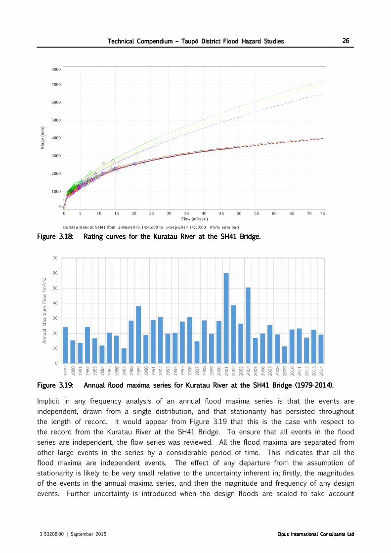
Technical Compendium Technical Compendium Technical Compendium Technical Compendium –––– TaupTaupTaupTaupō District Flood Hazard StudiesDistrict Flood Hazard StudiesDistrict Flood Hazard StudiesDistrict Flood Hazard Studies 26262626
3-53208.00 | September 2015 Opus International Consultants LtdOpus International Consultants LtdOpus International Consultants LtdOpus International Consultants Ltd
Figure Figure Figure Figure 3333....18181818:::: Rating curves for the Rating curves for the Rating curves for the Rating curves for the Kuratau River at the SH41 BridgeKuratau River at the SH41 BridgeKuratau River at the SH41 BridgeKuratau River at the SH41 Bridge....
Figure Figure Figure Figure 3333....19191919:::: Annual Annual Annual Annual flood flood flood flood maxima maxima maxima maxima series for series for series for series for Kuratau River at the SH41 Bridge Kuratau River at the SH41 Bridge Kuratau River at the SH41 Bridge Kuratau River at the SH41 Bridge (19(19(19(1979797979----2014).2014).2014).2014).
Implicit in any frequency analysis of an annual flood maxima series is that the events are
independent, drawn from a single distribution, and that stationarity has persisted throughout
the length of record. It would appear from Figure 3.19 that this is the case with respect to
the record from the Kuratau River at the SH41 Bridge. To ensure that all events in the flood
series are independent, the flow series was reviewed. All the flood maxima are separated from
other large events in the series by a considerable period of time. This indicates that all the
flood maxima are independent events. The effect of any departure from the assumption of
stationarity is likely to be very small relative to the uncertainty inherent in; firstly, the magnitudes
of the events in the annual maxima series, and then the magnitude and frequency of any design
events. Further uncertainty is introduced when the design floods are scaled to take account
0 5 10 15 20 25 30 35 40 45 50 55 60 65 70 75
0
1000
2000
3000
4000
5000
6000
7000
8000
Flow (m³/sec)
Kuratau River at SH41 from 2-Mar-1976 14:45:00 to 1-Sep-2014 14:30:00 0%% error bars
Sta
ge (
mm
)
0
10
20
30
40
50
60
70
1979
1980
1981
1982
1983
1984
1985
1986
1987
1988
1989
1990
1991
1992
1993
1994
1995
1996
1997
1998
1999
2000
2001
2002
2003
2004
2005
2006
2007
2008
2009
2010
2011
2012
2013
2014
Annual Maximum Flow (m³/s)

Technical Compendium Technical Compendium Technical Compendium Technical Compendium –––– TaupTaupTaupTaupō District Flood Hazard StudiesDistrict Flood Hazard StudiesDistrict Flood Hazard StudiesDistrict Flood Hazard Studies 27272727
3-53208.00 | September 2015 Opus International Consultants LtdOpus International Consultants LtdOpus International Consultants LtdOpus International Consultants Ltd
of the difference in catchment area between SH41 and Lake Taupō. It is problematic that if
the assumption of stationarity is not valid then any robust frequency analysis would not be
possible.
An updated frequency analysis of the Kuratau River at the SH41 Bridge annual flood maxima
series was undertaken using the extended record up until the end 2014 (Figure 3.20 & Figure
3.21).
Figure Figure Figure Figure 3333....20202020:::: L moment analysis for L moment analysis for L moment analysis for L moment analysis for Kuratau River at the SH41 BridgeKuratau River at the SH41 BridgeKuratau River at the SH41 BridgeKuratau River at the SH41 Bridge annual flood maxima seriesannual flood maxima seriesannual flood maxima seriesannual flood maxima series....
Figure Figure Figure Figure 3333....21212121:::: Frequency analysis for Frequency analysis for Frequency analysis for Frequency analysis for Kuratau River at the SH41 BridgeKuratau River at the SH41 BridgeKuratau River at the SH41 BridgeKuratau River at the SH41 Bridge annual flood maxima seriesannual flood maxima seriesannual flood maxima seriesannual flood maxima series....
-0.2 -0.1 0.0 0.1 0.2 0.3 0.4 0.5 0.6 0.7
-0.1
0.0
0.1
0.2
0.3
0.4
0.5
Gumbel
GEV
Generalised Logistic
Generalised Pareto
Log Normal
Pearson Type 3
L-Moment Ratios: L-Kurtosis versus L-SkewnessFlow (m³/sec) at Kuratau River at SH41 from 14-Nov-1978 11:00 to 1-Oct-2014 00:00
1.0 0.5 0.2 0.1 0.05 0.02 0.01 0.005 0.002 0.001 0.0005 0.0002
0
10
20
30
40
50
60
70
80
90
100
kjihgfe
dcbaZYXWVU
TSRQPONMLKJ I H G
F E
D C
B
A
A-k Flow (m³/sec) at Kuratau River at SH41 From 14-Nov-1978 11:00:00 to 1-Oct-2014 00:00:00 GEV Distribution: Location = 18.6 Scale = 7.02 Shape = -0.108 GenLog Distribution: Location = 21.4 Scale = 4.93 Shape = -0.241 GenPareto Distribution: Location = 11.4 Scale = 14.8 Shape = 0.222 Normal Distribution: Mean = 3.07 Std.Dev = 0.723 Pearson3 Distribution: Location = 23.5 Scale = 10.3 Shape = 1.45 Gumbel Distribution: Location = 19 Scale = 7.84

Technical Compendium Technical Compendium Technical Compendium Technical Compendium –––– TaupTaupTaupTaupō District Flood Hazard StudiesDistrict Flood Hazard StudiesDistrict Flood Hazard StudiesDistrict Flood Hazard Studies 28282828
3-53208.00 | September 2015 Opus International Consultants LtdOpus International Consultants LtdOpus International Consultants LtdOpus International Consultants Ltd
The L moment analysis indicates that a Generalised Logistic statistical distribution best
represents the annual flood maxima series for the Kuratau River at the SH41 Bridge. However,
when reviewing the various statistical distributions, the Generalised Logistic distribution appears
to have an unrealistic shape. Peak discharges appear to increase at an increasing rate with
decreasing AEP of the event (Figure 3.21). Flood magnitudes do not appear to ‘flatten off’ with
increasing recurrence interval as is normally the case for floods in New Zealand. The statistical
distributions with the more realistic ‘fit’ to the annual flood maxima series are either the GEV
or PE3. The use of a GEV distribution produces slightly conservative (i.e. higher) estimates of
the magnitudes of various design flood events (Table 3.10). These design flood estimates are
considered the most reliable when assessing the potential flood hazard.
Table Table Table Table 3333....10101010:::: Results of Results of Results of Results of a a a a frequency analysis frequency analysis frequency analysis frequency analysis of the annual flood maxima series of the annual flood maxima series of the annual flood maxima series of the annual flood maxima series for for for for the the the the Kuratau Kuratau Kuratau Kuratau
River at the SH41 Bridge River at the SH41 Bridge River at the SH41 Bridge River at the SH41 Bridge 1978197819781978----2014 (m³/s)2014 (m³/s)2014 (m³/s)2014 (m³/s)....
ARIARIARIARI GEVGEVGEVGEV GeneralisedGeneralisedGeneralisedGeneralised
LogisticLogisticLogisticLogistic
GeneralisedGeneralisedGeneralisedGeneralised
ParetoParetoParetoPareto
LogLogLogLog
NormalNormalNormalNormal PE3PE3PE3PE3 GumbelGumbelGumbelGumbel
2.332.332.332.33 23 23 23 23 23 24
5555 30 30 31 30 31 31
10101010 37 36 38 36 37 37
20202020 43 43 44 42 44 42
50505050 53 53 50 50 52 50
100100100100 60 63 54 56 57 55
It should be noted that the difference between the magnitude of the 1%AEP event assuming a
GEV statistical distribution is only 2.4m³/s lower than the highest estimate, and only 6.5m³/s
higher than the lowest estimate i.e. the difference is only about ±7%. Given the uncertainties
inherent in estimating the magnitudes of various design flood events, these differences are not
significant and would have no effect on any flood hazard assessment.
The results from a frequency analysis of the annual flood maxima series from the Kuratau River
at the SH41 Bridge, assuming a GEV statistical distribution, were scaled by the difference in
area to the power of 0.8 to estimate the discharge at Lake Taupō (Table 3.11).
Table Table Table Table 3333....11111111:::: RRRResults of frequency analysis for esults of frequency analysis for esults of frequency analysis for esults of frequency analysis for Kuratau River at Kuratau River at Kuratau River at Kuratau River at mouthmouthmouthmouth (m³/s)(m³/s)(m³/s)(m³/s)....
ARIARIARIARI
Kuratau Kuratau Kuratau Kuratau River at the River at the River at the River at the
SH41 Bridge SH41 Bridge SH41 Bridge SH41 Bridge (119(119(119(119km²km²km²km²))))
Kuratau Kuratau Kuratau Kuratau River at River at River at River at
mouth mouth mouth mouth (198(198(198(198km²)km²)km²)km²)
2.332.332.332.33 23 34
5555 30 45
10101010 37 55
20202020 43 65
50505050 53 79
100100100100 60 91

Technical Compendium Technical Compendium Technical Compendium Technical Compendium –––– TaupTaupTaupTaupō District Flood Hazard StudiesDistrict Flood Hazard StudiesDistrict Flood Hazard StudiesDistrict Flood Hazard Studies 29292929
3-53208.00 | September 2015 Opus International Consultants LtdOpus International Consultants LtdOpus International Consultants LtdOpus International Consultants Ltd
Despite some inherent uncertainty in the estimates of the magnitude of flood flows, those
derived from the Kuratau River at the SH41 Bridge record, and then scaled downstream to Lake
Taupō, are considered robust. They are the best available for any flood hazard analysis and
hydraulic modelling.
Whareroa Stream
The only flow series on Whareroa Stream to assess the flood risk is from a site called “FishTrap”.
The site is operated and maintained by the Waikato Regional Council. A discussion on this
flow record is available in Paine and Smith (2012c). Flows were monitored for a 3-year period
starting in 1977, and then since 2002. Consequently, the combined flow record is now about
15 years long. This record is therefore of limited duration for a robust frequency analysis;
particularly for larger and less frequent events. The relatively short flow record from Whareroa
Stream acts as a constraint on the accuracy and confidence that can be placed in estimates
of the potential magnitude of various design flood events, and consequently the results of any
flood modelling. To mitigate any potential effects of this uncertainty, a comparison with the
flow record from the adjacent catchment i.e. Kuratau at SH41, scaled to account for differences
in catchment area, is also provided.
The flow record has 30 periods of missing data; including the 22 year gap between 1980 and
2002. Over the remainder of the flow record there are missing data for a total of approximately
6135 hours (i.e. 256 days). The characteristics of these gaps are summarised in Table 3.12.
Table Table Table Table 3333....12121212:::: Gap analysis of Gap analysis of Gap analysis of Gap analysis of Whareroa at Fish Trap Whareroa at Fish Trap Whareroa at Fish Trap Whareroa at Fish Trap flow recordflow recordflow recordflow record....
DurationDurationDurationDuration Number of gapsNumber of gapsNumber of gapsNumber of gaps Total hoursTotal hoursTotal hoursTotal hours
>1 week 9 195423
<1 week 17 1182
< 1day 1 15
The rating curves for the Whareroa at Fish Trap are shown in Figure 3.22; together with the
various gaugings used to define the curves. These data were provided by the Waikato Regional
Council.
There have been 73 flow gaugings between 2002 and 2014. The highest gauged flow of
2.36m³/s was on 15 September 2008, while the largest flow on record is estimated to have
been 13.66m³/s. The fact that the highest gauged flow is only 17% of the largest flow on
record indicates considerable uncertainty regarding the accuracy and reliability of the estimates
of peak discharge during large flood events. This uncertainty has a potential impact on the
reliability of the annual flood maxima series, and the magnitude of any design flood events
derived from these data.
The annual maxima flood series from the Whareroa at Fish Trap is shown in Figure 3.23.
Although the available data are limited, there is no obvious longer term trend in either the
magnitudes or frequencies of large flood events. The annual flood maxima appear essentially

Technical Compendium Technical Compendium Technical Compendium Technical Compendium –––– TaupTaupTaupTaupō District Flood Hazard StudiesDistrict Flood Hazard StudiesDistrict Flood Hazard StudiesDistrict Flood Hazard Studies 30303030
3-53208.00 | September 2015 Opus International Consultants LtdOpus International Consultants LtdOpus International Consultants LtdOpus International Consultants Ltd
random. This is consistent with the lack of any trend apparent in the longer flow records from
the other tributaries to Lake Taupō.
Figure Figure Figure Figure 3333....22222222:::: Rating curves for the Rating curves for the Rating curves for the Rating curves for the Whareroa at Fish TrapWhareroa at Fish TrapWhareroa at Fish TrapWhareroa at Fish Trap....
Figure Figure Figure Figure 3333....23232323:::: Annual maxima flood series for Annual maxima flood series for Annual maxima flood series for Annual maxima flood series for Whareroa at Fish Trap Whareroa at Fish Trap Whareroa at Fish Trap Whareroa at Fish Trap (197(197(197(1978888----2014201420142014).).).).
Implicit in any frequency analysis of an annual flood maxima series is that the events are
independent, drawn from a single distribution, and that stationarity has persisted throughout
the length of record. It would appear from Figure 3.23 that this is the case with respect to
the flow record from the Whareroa at Fish Trap. To ensure that all events in the flood series
are independent, the flow series was reviewed. All the flood maxima are separated from other
large events in the series by a considerable period of time. This indicates that all the flood
maxima are independent events. The effect of any departure from the assumption of stationarity
0
2
4
6
8
10
12
14
16
1978
1979
1980
1981
1982
1983
1984
1985
1986
1987
1988
1989
1990
1991
1992
1993
1994
1995
1996
1997
1998
1999
2000
2001
2002
2003
2004
2005
2006
2007
2008
2009
2010
2011
2012
2013
2014
Annual Maximum Flow (m³/s)

Technical Compendium Technical Compendium Technical Compendium Technical Compendium –––– TaupTaupTaupTaupō District Flood Hazard StudiesDistrict Flood Hazard StudiesDistrict Flood Hazard StudiesDistrict Flood Hazard Studies 31313131
3-53208.00 | September 2015 Opus International Consultants LtdOpus International Consultants LtdOpus International Consultants LtdOpus International Consultants Ltd
is likely to be very small relative to the uncertainty inherent in; firstly, the magnitudes of the
flood events in the annual maxima series, and then the magnitude and frequency of any design
events. It is problematic that if the assumption of stationarity is not valid then any robust
frequency analysis would not be possible.
An updated frequency analysis of the annual flood maxima series from the Whareroa at Fish
Trap was undertaken using the extended record up until the end of 2014. This included an
analysis of the L moments (Figure 3.24), and the appropriateness of various different statistical
distributions when modelling the annual flood maxima series (Figure 3.25).
Figure Figure Figure Figure 3333....24242424:::: L moment analysis of the L moment analysis of the L moment analysis of the L moment analysis of the Whareroa at Fish TrapWhareroa at Fish TrapWhareroa at Fish TrapWhareroa at Fish Trap annual flood maxima series.annual flood maxima series.annual flood maxima series.annual flood maxima series.
Figure Figure Figure Figure 3333....25252525:::: Frequency analysis of the Frequency analysis of the Frequency analysis of the Frequency analysis of the Whareroa at Fish TrapWhareroa at Fish TrapWhareroa at Fish TrapWhareroa at Fish Trap annual flood maxima series.annual flood maxima series.annual flood maxima series.annual flood maxima series.
-0.2 -0.1 0.0 0.1 0.2 0.3 0.4 0.5 0.6 0.7
-0.1
0.0
0.1
0.2
0.3
0.4
0.5
Gumbel
GEV
Generalised Logistic
Generalised Pareto
Log Normal
Pearson Type 3
L-Moment Ratios: L-Kurtosis versus L-SkewnessFlow (m³/s) at Whareroa at Fish Trap from 26-Sep-1977 14:45 to 22-Jan-2015 12:20
1.0 0.5 0.2 0.1 0.05 0.02 0.01 0.005 0.002 0.001 0.0005 0.0002
02
4
6
8
10
12
14
16
18
20
22
24
26
2830
RQP
ONMLKJ I H
GF E
D
CB
A
A-R Flow (m³/s) at Whareroa at Fish Trap From 26-Sep-1977 14:45:00 to 22-Jan-2015 12:20:00 GEV Distribution: Location = 4.58 Scale = 3.04 Shape = 0.0311 GenLog Distribution: Location = 5.74 Scale = 1.98 Shape = -0.15 GenPareto Distribution: Location = 1.16 Scale = 7.52 Shape = 0.478 Normal Distribution: Mean = 1.76 Std.Dev = 1.08 Pearson3 Distribution: Location = 6.24 Scale = 3.73 Shape = 0.913 Gumbel Distribution: Location = 4.53 Scale = 2.96

Technical Compendium Technical Compendium Technical Compendium Technical Compendium –––– TaupTaupTaupTaupō District Flood Hazard StudiesDistrict Flood Hazard StudiesDistrict Flood Hazard StudiesDistrict Flood Hazard Studies 32323232
3-53208.00 | September 2015 Opus International Consultants LtdOpus International Consultants LtdOpus International Consultants LtdOpus International Consultants Ltd
The L moment analysis indicates that a PE3 statistical distribution best represents the annual
flood maxima series from Whareroa Stream at Fish Trap. Reviewing the various statistical
distributions shows that the assumption of a PE3 distribution, or a GEV distribution, provides a
slightly conservative (i.e. higher) estimate of the magnitude of the 1%AEP design flood event.
Estimates of the magnitudes of various design flood events, assuming several different statistical
distributions, are listed in Table 3.13. The PE3 results are highlighted and are considered the
more reliable; although they are almost identical to those assuming a GEV distribution. The
difference between the magnitudes of the 1%AEP flood event assuming a PE3 distribution is
6.3m³/s lower than the highest estimate, and 2.2m³/s higher than the lowest estimate. The
design flood estimates obtained assuming a Log Normal statistical distribution are significantly
higher than any other estimate and should be disregarded. Given the uncertainties inherent in
estimating the magnitudes of various design flood events, the uncertainty caused by the choice
of either the PE3 or GEV statistical distribution is not likely to have a significant impact on any
subsequent analysis.
Table Table Table Table 3333....13131313:::: Results of frequency analysis for Results of frequency analysis for Results of frequency analysis for Results of frequency analysis for Whareroa at Fish Trap Whareroa at Fish Trap Whareroa at Fish Trap Whareroa at Fish Trap 1971971971977777----2012012012015555 (m³/s)(m³/s)(m³/s)(m³/s)....
ARIARIARIARI GEVGEVGEVGEV GeneralisedGeneralisedGeneralisedGeneralised
LogisticLogisticLogisticLogistic
GeneralisedGeneralisedGeneralisedGeneralised
ParetoParetoParetoPareto
LogLogLogLog
NormalNormalNormalNormal PE3PE3PE3PE3 GumbelGumbelGumbelGumbel
2.332.332.332.33 6.3 6.3 6.4 6.0 6.3 6.2
5555 9.0 8.8 9.6 9.2 9.1 9.0
10101010 11.2 10.9 11.7 12.2 11.2 11.2
20202020 13.2 13.1 13.1 15.4 13.2 13.3
50505050 15.8 16.2 14.5 19.9 15.6 16.1
100100100100 17.6 18.8 15.1 23.6 17.3 18.2
As a result of the relatively short nature of the Whareroa at Fish Trap annual flood maxima
series, the results from the frequency analysis of the Kuratau at SH41, the adjacent catchment,
were also scaled as a function of catchment area (i.e. A0.8).
The estimated peak discharge during a 1%AEP event in Whareroa Stream derived by scaling
the results of a flood frequency analysis of the longer-term Kuratau River at SH41 Bridge flow
record by A0.8 is approximately twice as large as that obtained from the local flow series (Table
3.14). An extensive discussion of the reasons for this difference, and the potential effect of
the results on the assessment of the flood hazard is provided in Paine and Smith (2012c).
However, the incised nature and local topography of the lower Whareroa Stream means that
any ‘error’ in estimating the magnitude of design floods is likely to have little effect on the
results of any flood hazard assessment.

Technical Compendium Technical Compendium Technical Compendium Technical Compendium –––– TaupTaupTaupTaupō District Flood Hazard StudiesDistrict Flood Hazard StudiesDistrict Flood Hazard StudiesDistrict Flood Hazard Studies 33333333
3-53208.00 | September 2015 Opus International Consultants LtdOpus International Consultants LtdOpus International Consultants LtdOpus International Consultants Ltd
Table Table Table Table 3333....14141414:::: Results of frequency analysis for Results of frequency analysis for Results of frequency analysis for Results of frequency analysis for Kuratau River at Kuratau River at Kuratau River at Kuratau River at mouthmouthmouthmouth (m³/s)(m³/s)(m³/s)(m³/s)....
ARIARIARIARI
Kuratau Kuratau Kuratau Kuratau River at the River at the River at the River at the
SH41 Bridge SH41 Bridge SH41 Bridge SH41 Bridge (119km²)(119km²)(119km²)(119km²)
Whareroa at Whareroa at Whareroa at Whareroa at
Fish Trap Fish Trap Fish Trap Fish Trap scaled from scaled from scaled from scaled from
Kuratau at Kuratau at Kuratau at Kuratau at SH41SH41SH41SH41
(58.8km²)(58.8km²)(58.8km²)(58.8km²)
WhareroWhareroWhareroWhareroa at a at a at a at Fish Trap Fish Trap Fish Trap Fish Trap
from actual from actual from actual from actual recordrecordrecordrecord
2.332.332.332.33 23 13 6.3
5555 30 17 9.1
10101010 37 21 11.2
20202020 43 25 13.2
50505050 53 30 15.6
100100100100 60 34 17.3
4444 Hydraulic Hydraulic Hydraulic Hydraulic mmmmodellingodellingodellingodelling
The hydraulic modelling undertaken as part of the Taupō District Flood Study covered five
watercourses: the Tongariro River; Kuratau River; Hinemaiaia River; Whareroa Stream; and
Tokaanu Stream. The extents of each of the hydraulic models are described in the respective
‘Taupō District Flood Hazard Study’ reports (Maas & McConchie, 2011; Paine & Smith, 2012a;
Paine & Smith, 2012b; Smith et al., 2011; Paine & Smith, 2012c). The hydraulic modelling of
the Tongariro River is covered by its own separate report (Maas, 2009).
4.14.14.14.1 Modelling Modelling Modelling Modelling ssssoftwareoftwareoftwareoftware
All the computational hydraulic modelling was undertaken using “MIKE software” developed by
DHI Water and Environmental (formerly the Danish Hydraulic Institute and some other
organisations). MIKE hydrodynamic modelling software tools are widely used, throughout New
Zealand and internationally, to aid engineers and other professionals in the assessment and
management of river flooding. Hydrodynamic modelling allows the user (with enough input data)
to estimate water levels, flows, and velocities at discreet locations and points in time over the
duration of a flood. Effects on water level can be carried both upstream and downstream over
time and so these models are termed dynamic.
Hydrodynamic modelling tools are generally classified as either one-dimensional (1D) or two-
dimensional (2D). The difference between the two types of models relates to the mathematical
approach adopted to describe the river and floodplain.
4.24.24.24.2 1D and 2D model1D and 2D model1D and 2D model1D and 2D modelssss
One-dimensional models (e.g. MIKE11) generally represent the river or stream as a series of
cross-sections. Flow, velocity and depth are averaged across each cross-section of the river
channel or floodplain which comprises the model’s river network. There are various methods

Technical Compendium Technical Compendium Technical Compendium Technical Compendium –––– TaupTaupTaupTaupō District Flood Hazard StudiesDistrict Flood Hazard StudiesDistrict Flood Hazard StudiesDistrict Flood Hazard Studies 34343434
3-53208.00 | September 2015 Opus International Consultants LtdOpus International Consultants LtdOpus International Consultants LtdOpus International Consultants Ltd
to improve the answers given by averaging, but in essence a 1D model requires the user to
fully specify the direction of water flow. This assumption is generally good when flow is
predominantly uni-directional, such as in a well-defined river channel.
In a 2D hydrodynamic model (e.g. MIKE21) flow, velocity and depth are able to be calculated
across a near-horizontal planar surface. Localised values of flow velocity (averaged over the
depth) and depth are obtained across a grid network rather than over a channel cross-section.
This approach is especially useful when modelling flow across a floodplain where the horizontal
flow direction is difficult to predict. MIKE21 also more accurately simulates energy losses as
any flow moves across the floodplain than a 1D model. It can also estimate the energy losses
which occur when flow either re-enters or exits the main channel. Consequently, 2D models
are much more appropriate for modelling flow across floodplains.
The MIKE suite of hydrodynamic modelling software provides the following tools:
• MIKE11 – a 1D tool generally used to model flow within a defined uni-directional channel;
• MIKE21 – a 2D tool used to model flow across a floodplain or large channel where the
landscape can be represented by a ‘grid’ rather than cross-sections. Flow direction may
be difficult to predict, and there may be significant differences in flow depth, velocity and
direction between adjacent cells forming the grid. A two-dimensional MIKE21 model can
simulate multi-directional flow over a floodplain when combined with high-resolution
topographic information, such as that from a LiDAR survey; and
• MIKEFLOOD - is able to more realistically model a river-floodplain system where overtopping
of the riverbanks, and overland flow occurs. MIKEFLOOD dynamically links together a
one-dimensional MIKE11 model of a river channel with a two-dimensional MIKE21 model
of a floodplain.
With respect to the Taupō District Flood Study the flood hazard of the Tongariro River and
Tokaanu Stream was modelled in MIKE21. In these cases the channel was either large enough
to be represented as a ‘mesh’ of grid cells (e.g. the Tongariro River) or so small as to have no
significant effect of the flooding (e.g. Tokaanu Stream). In both cases the key concern was to
assess the flood risk to the floodplain rather than the river itself.
For the Kuratau River, Hinemaiaia River and the Whareroa Stream MIKEFLOOD was used to
combine a one-dimensional representation of the channel in MIKE11 with a two-dimensional
model of the floodplain in MIKE21.
MIKEFLOOD models are generally concerned with assessing potential inundation of the floodplain
rather than the flood hazard within the actual river channel. Consequently, the results from a
MIKEFLOOD model often do not include the actual channel. This was the case with respect to
the Tauranga Taupō River. The flood hazard of the actual river channel was therefore assessed
intuitively rather than as a function of the depth and velocity. Given the depth and velocity
within the active channel the flood hazard was assessed as ‘High’.

Technical Compendium Technical Compendium Technical Compendium Technical Compendium –––– TaupTaupTaupTaupō District Flood Hazard StudiesDistrict Flood Hazard StudiesDistrict Flood Hazard StudiesDistrict Flood Hazard Studies 35353535
3-53208.00 | September 2015 Opus International Consultants LtdOpus International Consultants LtdOpus International Consultants LtdOpus International Consultants Ltd
4.34.34.34.3 Level datumLevel datumLevel datumLevel datum
All ground levels, river and stream bed levels, lake levels, and predicted flood levels are
expressed in terms of mean sea level relative to the Moturiki datum. It should be noted,
however, that the flood hazard is essentially modelled using the ‘relative elevations’ of the river
and adjacent floodplain not the absolute height.
4.44.44.44.4 FloodFloodFloodFloodplain descriptionplain descriptionplain descriptionplain description
The Digital Terrain Models (DTMs) used in the modelling had a maximum spatial resolution of
5m. All the terrain models were based on the June-July 2006 LiDAR data supplied by
Environment Waikato. This was supplemented with later data provided by Taupō District Council
for two locations: in the vicinity of Waihi, towards the southern end of Lake Taupō; and the
foreshore adjacent to the Taupō township. All the LiDAR data has a spatial resolution of 1m
and a vertical accuracy of ±0.1m. The LiDAR information was used to provide a three-
dimensional model of the shoreline of Lake Taupō, and floodplain topography adjacent to
various rivers and streams. Using a 5m resolution DTM allowed relatively shorter computer run-
times without significantly reducing the model accuracy in terms of the prediction of flood levels
and extents.
4.54.54.54.5 LiDARLiDARLiDARLiDAR accuracyaccuracyaccuracyaccuracy
When raw LiDAR data are processed, part of the filtering process is to remove the effects of
any vegetation cover so that the data better represents the elevation of the ground surface.
Over heavily vegetated areas this is difficult and may lead to errors in the final inferred
topography, and any derived DTM.
The various algorithms used to process LiDAR data produce consistent data, with a high level
of reliability and accuracy. While dense tall vegetation can cause calibration problems, the
relative heights are consistent across the terrain model. Since a flood surface is developed
from the relative topographic information slight errors in the absolute height, usually within
±0.15m, have little quantifiable effect. LiDAR information is now the international standard for
generating terrain models, and consequently flood extents, across floodplains. That is, despite
the possibility of minor errors, LiDAR information is the best available for floodplain modelling.
The collection of LiDAR information does not extend deeper than approximately 10cm below
any water surface. Therefore in areas where there is an abrupt change in elevation close to
the shoreline of Lake Taupō, such as in the Western Bays, this leads to instability in any DTM
derived from the LiDAR information i.e. accurate elevation data for the lake edge are not
available because of the steep scarp. However, given the nature of the terrain where this is a
potential problem i.e. steep cliffs dropping to the lake, it has no effect on the assessed flood
risk.

Technical Compendium Technical Compendium Technical Compendium Technical Compendium –––– TaupTaupTaupTaupō District Flood Hazard StudiesDistrict Flood Hazard StudiesDistrict Flood Hazard StudiesDistrict Flood Hazard Studies 36363636
3-53208.00 | September 2015 Opus International Consultants LtdOpus International Consultants LtdOpus International Consultants LtdOpus International Consultants Ltd
4.64.64.64.6 River cRiver cRiver cRiver channelhannelhannelhannel descriptiondescriptiondescriptiondescription
No surveyed cross-sections were available for the various hydraulic models; except for the
Tongariro River as discussed in Maas (2009), and the Kuratau River as discussed in Smith et
al. (2011). The LiDAR elevation measurements are of the water surface at the time the data
were ‘captured’. Hence, the river bed and lake bed below the water surface was not represented
in the supplied data. Therefore the river bed needed to be ‘burnt’ into the DTM created from
the LiDAR information.
For the Tongariro River, the average bed levels at each cross-section over the 5.5km reach of
the river through Turangi were extracted from the previous MIKE11 model of the Tongariro River
(T&T, 2004) and used to adjust the DTM at the relevant locations.
The river bed ‘burnt’ into the MIKE21 model included all the current gravel shoals without
vegetation. This is because these shoals are considered likely to become mobile when there
are significant flows in the river i.e. during the large events considered during the flood hazard
analysis.
The volume of the channel of Tokaanu Stream below the water surface when the LiDAR was
captured was ignored. Given that the width and volume of water in the stream during low
flows, when the LiDAR was likely to have been captured, are very small relative to those during
the extreme events considered in this study, this assumption is reasonable. Any error caused
by this assumption is likely to be small when compared to the inherent uncertainty of other
inputs to the hydraulic model.
The Kuratau River contains a deep, narrow channel in places which is difficult to represent in
a two-dimensional grid. To do so requires an extremely high resolution (high number of grid
cells) model. To run such a model then requires prohibitively long computer processing time.
The LiDAR data was therefore augmented with cross-sections extracted from a previous Cheal
Consultants HEC-RAS model. These cross-sections were generated from a terrain model derived
from GPS survey contours.
The cross-sections derived from LiDAR data were compared to those where survey data were
also available. A conservative depth value was then added to the LiDAR-sourced channel data.
This was to ensure a smooth transition along the channel between reaches where survey data
were available (lower channel), and other reaches where only LiDAR data were available.
For the Hinemaiaia River hydraulic model, cross-sections were extracted from a high resolution
1.0m DTM, and then checked carefully against the original LiDAR data used to construct the
DTM. These cross-sections were then implemented in the one-dimensional MIKE11 portion of
the hydraulic model.
The same process was followed for the Whareroa Stream hydraulic model, but using a higher
resolution 0.5m DTM.

Technical Compendium Technical Compendium Technical Compendium Technical Compendium –––– TaupTaupTaupTaupō District Flood Hazard StudiesDistrict Flood Hazard StudiesDistrict Flood Hazard StudiesDistrict Flood Hazard Studies 37373737
3-53208.00 | September 2015 Opus International Consultants LtdOpus International Consultants LtdOpus International Consultants LtdOpus International Consultants Ltd
4.74.74.74.7 Lake Lake Lake Lake TaupTaupTaupTaupō descriptiondescriptiondescriptiondescription
Lake Taupō forms the downstream boundary for all the models so it was necessary to represent
part of the lake in each model. This was done by adding the bed level of Lake Taupō to each
DTM. The lake bed levels were based on available bathymetric data.
4.84.84.84.8 VegetationVegetationVegetationVegetation effectseffectseffectseffects
When raw LiDAR data are processed, part of the filtering process is to remove the effects of
any vegetation cover. Over heavily vegetated areas this is difficult and may lead to errors in
the final inferred topography. In some areas, the original LiDAR data had not been corrected
adequately for the effect of floodplain vegetation.
For the Tongariro River model this led to water levels that were considerably higher than those
predicted by the MIKE11 model for the calibration event (T&T, 2004). The DTM was therefore
lowered over the floodplain to more accurately reflect the ground levels in these locations.
The corrections made to the DTM were primarily based on a comparison between corresponding
cross-sections from the MIKE21 DTM and cross-sections from the MIKE11 model (T&T, 2004).
For the other models, no additional adjustments were made for the effects of vegetation.
4.94.94.94.9 StructuresStructuresStructuresStructures
Stopbanks on the Tongariro River were included in the model through the DTM. Stopbanks
constructed prior to the calibration event (29 February 2004) show up in the model bathymetry
and were therefore all assumed to have been included in the LiDAR data. These were not
checked further, nor amended. Stopbanks constructed after the calibration event were also
included in the LiDAR data. Therefore these were removed from the DTM when calibrating the
hydraulic model against the 2004 flood event.
Once the model was calibrated, all the stopbanks constructed since 29 February 2004 were
added back into the DTM to represent the present (2008) situation. Care was taken to ensure
that each stopbank formed a continuous linear feature in the DTM. The levels used for each
stopbank were based on as-built drawings provided by the Waikato Regional Council. No
surveying of the stopbanks was undertaken for this study and the as-built drawings were
assumed to be correct.
Consideration was given to modelling the flow through the specific design characteristics of the
SH41 Bridge over Tokaanu Stream. However, investigation of preliminary model results showed
that flood levels remain well below the soffit of the bridge. Also, the pier arrangement (one
narrow pier in the centre of the stream) is such that no undue flow energy losses occur which
would require special treatment of the bridge within the hydraulic model. Losses resulting from
contraction and expansion of flow through a narrow opening were accounted for by default by
using a two-dimensional modelling approach. Other small bridges were not considered to require

Technical Compendium Technical Compendium Technical Compendium Technical Compendium –––– TaupTaupTaupTaupō District Flood Hazard StudiesDistrict Flood Hazard StudiesDistrict Flood Hazard StudiesDistrict Flood Hazard Studies 38383838
3-53208.00 | September 2015 Opus International Consultants LtdOpus International Consultants LtdOpus International Consultants LtdOpus International Consultants Ltd
special treatment as they are located within a highly vegetated main channel which was modelled
with a relatively high resistance factor.
No additional adjustments to include specific structures were made to the Kuratau River,
Hinemaiaia River and Whareroa Stream hydraulic models.
4.104.104.104.10 Surface roughnessSurface roughnessSurface roughnessSurface roughness
Each land use in the model was assigned a Manning’s n value to represent the ground surface
roughness. The following roughness values were used in the models:
Table Table Table Table 4444....1111:::: Values of Manning’s Values of Manning’s Values of Manning’s Values of Manning’s n n n n roughness values used in the MIKE21 modelsroughness values used in the MIKE21 modelsroughness values used in the MIKE21 modelsroughness values used in the MIKE21 models....
Land coverLand coverLand coverLand cover Manning’s nManning’s nManning’s nManning’s n Manning’s M Manning’s M Manning’s M Manning’s M
(1/n)(1/n)(1/n)(1/n)
River bed 0.03 33.33
Trees/vegetation along banks 0.07 14.29
Floodplain trees 0.10 10.00
Floodplain pasture 0.03 33.33
Floodplain delta grass 0.05 20.00
Urban floodplain areas 0.15 6.67
Streets/roads 0.025 40.00
The land use was determined from aerial photography and known land uses. The Manning’s n
value for each land use was estimated using values reported in standard literature references,
past experience, and knowledge obtained from the previous calibration of the Tongariro River
hydraulic model (Maas, 2009).
The relatively higher Manning’s n value for ‘Urban floodplain areas’ accounts for the resistance
to flow caused by buildings in the urban centres.
4.114.114.114.11 Boundary Boundary Boundary Boundary cccconditionsonditionsonditionsonditions
To produce the predicted flood extents for a 1%AEP design flood event on each of the rivers
modelled, the 100-year peak discharge was applied to the model at the upstream end and the
1%AEP level of Lake Taupō was applied to the downstream end.
This combination of extreme events (i.e. a 1%AEP flood and a 1%AEP lake level) has a lower
effective probability of exceedance than ‘once in 100 years’. However, the level of Lake Taupō
changes very slowly, and by only a very small amount, with decreasing frequency of an event.
For example, the lake level changes only by 14cm between a 10%AEP event and a 1%AEP
event. Any effect of this relatively small change in lake level is within the resolution of the
hydraulic models.

Technical Compendium Technical Compendium Technical Compendium Technical Compendium –––– TaupTaupTaupTaupō District Flood Hazard StudiesDistrict Flood Hazard StudiesDistrict Flood Hazard StudiesDistrict Flood Hazard Studies 39393939
3-53208.00 | September 2015 Opus International Consultants LtdOpus International Consultants LtdOpus International Consultants LtdOpus International Consultants Ltd
4.124.124.124.12 Assumptions Assumptions Assumptions Assumptions and and and and uuuuncertaintyncertaintyncertaintyncertainty
There are a number of assumptions necessary during the construction of the various hydraulic
models. These include simplifications of reality during model build, assumptions regarding the
suitability of provided data, and the type of vegetation and materials present. These assumptions
are discussed below:
• The Manning’s n values applied for each of the different types of surface roughness in
the models were refined during the calibration of the Tongariro River hydraulic model
(Maas, 2009). Manning’s n values for different surface roughness types in the other
models were assigned based on values from standard references, past experience and
local knowledge;
• The materials and vegetation present during the survey/site visit/aerial photography are
assumed to be typical of the materials in the channel, and on the banks, at all times of
year and represent the worst case;
• The measured lake level data are assumed to be accurate as they are regularly audited
and subject to continuous scrutiny and peer-review;
• LiDAR data does not provide information beneath water bodies such as lakes, rivers and
ponds. In the hydraulic models where this was adjusted using information from other
sources, the data have been assumed to be correct;
• For the hydraulic models where the portion of wetted channels beneath the water surface
was ignored in constructing a DTM, any baseflow is likely to occupy only a very small
proportion of the total channel volume active during a large flood. This assumption is
reasonable and any resulting error in flood level predictions is likely to be small when
compared to the inherent uncertainty of other inputs to the hydraulic model;
• When LiDAR information is processed, algorithms are used to adjust elevation values to
remove or smooth out the effects of vegetation. Over heavily vegetated areas this is
difficult and may lead to errors in the provided LiDAR data. Other than the Tongariro
model where, in some areas, the elevation of the DTM has been manually adjusted during
the calibration process, the DTMs were assumed to be accurate;
• The 1%AEP flow and lake levels have been incorporated into the models to provide the
design scenario flood inundation extents. This combination would be a rare event and
has a lower probability than 1 in 100 years. Therefore the model results are conservative;
• The cross-sections defining the main river or stream channel in each model are assumed
to remain unchanged over the course of a flood. In reality, the river or stream bed
sediment material will be mobilised in large floods. However, the assumption of a “fixed”
bed will generally be conservative; and

Technical Compendium Technical Compendium Technical Compendium Technical Compendium –––– TaupTaupTaupTaupō District Flood Hazard StudiesDistrict Flood Hazard StudiesDistrict Flood Hazard StudiesDistrict Flood Hazard Studies 40404040
3-53208.00 | September 2015 Opus International Consultants LtdOpus International Consultants LtdOpus International Consultants LtdOpus International Consultants Ltd
• The flood inflows to each model assumed steady flows rather than unsteady flow flood
discharge hydrographs. This use of a constant steady flow makes no difference to flood
level predictions where rivers or streams are hydraulically steep and where there is minimal
channel storage. Such characteristics are typical of all the rivers and streams draining
to Lake Taupō which were modelled.
There is some uncertainty common to all hydraulic models. This is because of the difficulty in
defining real world processes precisely by mathematical expressions, and because of the
assumptions made regarding model parameters and inputs. For this study, however, the
assumptions made to counter or allow for this uncertainty are considered to produce results
that are conservative but still realistic. Tests were carried out to assess the sensitivity of the
model predictions to parameters for which there is greater uncertainty regarding their values.
The results of these sensitivity tests confirmed the appropriateness of the predicted flood hazard
zone in each case.
4.134.134.134.13 NonNonNonNon----contiguous areas contiguous areas contiguous areas contiguous areas –––– riverriverriverriver----based floodingbased floodingbased floodingbased flooding
The 2-D hydraulic modelling within MIKE21 and MIKEFLOOD assesses the movement of water
across a network of cells. In the various models used for the Taupō District Flood Hazard
Study cell sizes were either 2m or 5m depending on the model extent and situation. The final
results were presented within a common reference grid of 5m.
Although the model consists of a network of cells, flooding is only shown when the depth of
water flowing over the ground surface represented by the cell is greater than 3cm. Consequently,
it is possible to have water flowing over the surface, but the area not appearing at risk of
flooding, as long as any water is less than 3cm deep.
The effect of this is that it is possible to have what appear to be non-contiguous areas of
flooding i.e. areas where water depths exceed 3cm but which are separated from other areas
of flooding by zones of very shallow surface flow. Although these areas appear to be non-
contiguous on the flood hazard map, they are actually connected by zones of shallow surface
runoff and flooding.
4.144.144.144.14 Tongariro River model updateTongariro River model updateTongariro River model updateTongariro River model update
The digital terrain model used for the flood hazard assessment of the Tongariro River, reported
in Maas (2009) and Maas & McConchie (2011), was derived from LiDAR information flown in
June-July 2006 and supplied by Waikato Regional Council. The LiDAR topographic information
was combined with surveyed river cross-sections to establish a two-dimensional MIKE21 model.
The model covers an area of approximately 7.8km by 11.5km, and extends 19km downstream
from Poutu Pool to Lake Taupo.
The digital terrain model was initially adjusted by removing certain stopbanks so that it reflected
the river and its floodplain prior to the 29 February 2004 flood. The model was calibrated

Technical Compendium Technical Compendium Technical Compendium Technical Compendium –––– TaupTaupTaupTaupō District Flood Hazard StudiesDistrict Flood Hazard StudiesDistrict Flood Hazard StudiesDistrict Flood Hazard Studies 41414141
3-53208.00 | September 2015 Opus International Consultants LtdOpus International Consultants LtdOpus International Consultants LtdOpus International Consultants Ltd
against this flood event to ensure that all the parameters were appropriate and the results
realistic.
All the stopbanks constructed since February 2004 were then added to the pre-29 February
2004 digital terrain model, using information from the ‘as built’ drawings, so that the model
represented the present (i.e. 2009) situation. It is the results from this model which are reported
in Maas (2009) and Maas & McConchie (2011).
As part of a ‘Service Level Review’ Waikato Regional Council used the MIKE21 model with the
same parameters and boundary conditions (Grant, 2014). Two changes, however, were made.
These were:
• Using a flood hydrograph rather than a constant flood discharge; and
• Updating the representation of the stopbanks within the model using their actual surveyed
heights.
These changes, particularly the inclusion of what are essentially slightly higher stopbanks,
resulted in some changes to the pattern of flooding previously presented in Maas (2009) and
Maas & McConchie (2011).
To ensure that the latest information is used to inform the District planning process, the results
from this latest modelling have been adopted (i.e. those from Grant, 2014). These results are
considered to best represent current conditions likely to affect the flood risk to land adjacent
to the Tongariro River.
5555 Waves runWaves runWaves runWaves run----up analysisup analysisup analysisup analysis
5.15.15.15.1 Model adoptedModel adoptedModel adoptedModel adopted
Wave run-up around Lake Taupō has been estimated previously by Hicks et al. (2000) using the
hindcast model ‘LakeWave’. Output from the model was used successfully to predict lakeshore
geomorphic processes, shoreline erosion, and near-shore flooding.
LakeWave, however, has a number of limitations, including:
a. It has no nearshore dissipation of wave energy, and is therefore liable to over-estimate
wave run-up on shelving shores; and
b. It does not formally refract or diffract waves other than an empirical exposure weighting
on the effective fetch. Therefore the results are less reliable within embayed beaches.
Constraints relating to the Taupō District Flood Study meant that it was not feasible to develop
a more sophisticated model (e.g. SWAN) for assessing the potential for wave run-up around the
entire shoreline. Likewise the expense of developing a more sophisticated model could not be
justified. Irrespective of the model used to assess wave run-up at the District-scale, it is likely

Technical Compendium Technical Compendium Technical Compendium Technical Compendium –––– TaupTaupTaupTaupō District Flood Hazard StudiesDistrict Flood Hazard StudiesDistrict Flood Hazard StudiesDistrict Flood Hazard Studies 42424242
3-53208.00 | September 2015 Opus International Consultants LtdOpus International Consultants LtdOpus International Consultants LtdOpus International Consultants Ltd
that the results would still not be ‘accurate’ when enlarged to the scale of specific sites or
properties.
Consequently the approach adopted for the Taupō District Flood Study was to continue to use
LakeWave, but recognise fully its constraints and limitations when reviewing and applying the
results within the context of the District Plan.
While LakeWave has limitations as listed above, a qualitative assessment of the accuracy of the
model was undertaken by Hicks et al. (2000). They concluded that the agreement between
modelled and actual wave conditions was “quite reasonable”. At a broader scale they also
found qualitative agreement between the modelled run-up height and the amount of surf
observed at the time.
Subsequently, it was recognised by Opus (2008) that LakeWave functions acceptably at the
broad scale but that the results may be limited within small embayments where wave condition
are strongly affected by refraction and diffraction.
5.25.25.25.2 Alternative modelsAlternative modelsAlternative modelsAlternative models
SWAN2D is a more recent software model which can account for detailed bathymetric variations
around the shoreline. However, constraints on existing data availability, and data resolution,
would necessitate significant expenditure to realise any advantages over the results from
LakeWave.
A more sophisticated modelling approach, such as SWAN2D, could be explored in the future.
In particular, it might be appropriate for site-specific studies at critical locations highlighted by
the District-scale assessment using LakeWave.
5.35.35.35.3 Model inputsModel inputsModel inputsModel inputs
Representative beach characteristics used in Opus (2008) were initially a standard beach slope
of 7 degrees and a sediment size of 2mm. These parameters were used to provide estimates
of indicative potential wave run-up around the entire shoreline of the lake. The shoreline was
then refined into the ten distinct wave run-up environments; within which similar wave run-up
behaviour can be expected.
The considerable spatial variability in wave run-up around the shoreline means that the single
value was not appropriate when quantifying the wave run-up in each of the ten zones. The
complexity of the system, and constraints of the project, however meant that detailed individual
site analysis was impractical. Therefore the wave run-up at ten sites was analysed using site-
specific values of beach-face slope as detailed in Hicks et al. (2000). These locations were:
Taupō Beach (slope 0.12); Five Mile Bay (slope 0.13); Waitahanui (slope 0.12); Hatepe (slope
0.16); Te Rangaiita (slope 0.13); Waihi (slope 0.13); Kuratau (slope 0.14); Whanganui Bay (0.13);
Kinloch (slope 0.145); and Acacia Bay (slope 0.15). Sediment size, however, was assumed
constant at 2mm across all the sites. This was because the majority of these sites were

Technical Compendium Technical Compendium Technical Compendium Technical Compendium –––– TaupTaupTaupTaupō District Flood Hazard StudiesDistrict Flood Hazard StudiesDistrict Flood Hazard StudiesDistrict Flood Hazard Studies 43434343
3-53208.00 | September 2015 Opus International Consultants LtdOpus International Consultants LtdOpus International Consultants LtdOpus International Consultants Ltd
described as being composed of coarse or gritty sand with some gravel, and more detailed
size descriptions were not available.
5.45.45.45.4 Wind dataWind dataWind dataWind data
The use of the Taupō Airport wind record as being representative of the entire lake is likely to
have produced conservative estimates of run-up at the southern end of the lake. However, the
lack of any high resolution long-term wind record from Turangi, or anywhere at the southern
end of the lake, precluded the use of an alternative record when analysing wave run-up in that
vicinity.
The shorter wind record from Turangi which does exist shows more calm periods and less
severe extremes than at Taupō Airport. Therefore the wave run-up around the southern shoreline
is likely to be over-predicted. This is not considered to be a significant issue because of the
District-scale of the analysis, and the inherent advantages of being conservative rather than
under-estimating the risk. It should also be noted that wave run-up is only one element of the
hazard assessment at any location. Consequently any effect from over-estimating wave run-up
is mitigated and moderated in the final analysis of flood risk at any location.
The approach adopted in the Taupō District Flood Study is consistent with that adopted in
Hicks et al. (2000), Hicks (2006) and Macky & Bowler (1998). Those studies concluded:
The Taupō airport wind record was assumed to be representative of the whole lake.
In fact, the short wind record from Turangi shows that the southern shore experiences
more calm periods, and its extremes are less severe than at Taupō Airport (Macky
& Bowler, 1998). Given this, the wind-wave modelling results presented in the
following sections will over-predict the wave energy around the southern shore;
although the magnitude/frequency estimates are probably still reasonable (Hicks,
2006).
5.55.55.55.5 CalibrationCalibrationCalibrationCalibration
There are currently no empirical studies of the waves and wave run-up on Lake Taupō. It is
therefore not possible to establish an empirical relationship between the wind regime and the
resultant wave and wave run-up response. However, a qualitative calibration of the modelled
wave run-up has been done using photographic evidence e.g. Hicks et al. (2000) and Hicks
(2006). In addition, field evidence of extreme water levels; such as erosion trim lines, vegetation
edge lines, and beach ridge crests etc. can be used to verify the estimates of effective water
level and their effect at the shore.
Therefore the vegetation edge lines and beach ridge crests reported in Hicks et al. (2000) and
Cheal (2012 & 2013) have been compared to the modelled effective water levels (i.e. a
combination of lake level and wave run-up) for verification purposes.

Technical Compendium Technical Compendium Technical Compendium Technical Compendium –––– TaupTaupTaupTaupō District Flood Hazard StudiesDistrict Flood Hazard StudiesDistrict Flood Hazard StudiesDistrict Flood Hazard Studies 44444444
3-53208.00 | September 2015 Opus International Consultants LtdOpus International Consultants LtdOpus International Consultants LtdOpus International Consultants Ltd
Grigg (2010 & 2011) provide useful qualitative records of flood and wave damage during specific
storms. However, there are no vertical elevations recorded against the damage at specific sites.
These data could therefore not be used for robust calibration purposes.
Table 5.1 includes the elevations of these various indicators of ‘wave attack’. These are overlain
on the estimated effective water levels for each site (Figure 5.1 through Figure 5.9). There are
no surveyed levels for Whanganui Bay therefore wave run-up that site could not be calibrated.
Table Table Table Table 5555....1111:::: Levels indicative of extreme effective Levels indicative of extreme effective Levels indicative of extreme effective Levels indicative of extreme effective waterwaterwaterwater levels around Lake levels around Lake levels around Lake levels around Lake TaupTaupTaupTaupō fromfromfromfrom Hicks Hicks Hicks Hicks et et et et al.al.al.al. (2000) and Cheal (2012 & 2013).(2000) and Cheal (2012 & 2013).(2000) and Cheal (2012 & 2013).(2000) and Cheal (2012 & 2013).
Hicks Hicks Hicks Hicks et al. (2000)et al. (2000)et al. (2000)et al. (2000) Cheal Cheal Cheal Cheal (2012)(2012)(2012)(2012) Cheal (2013)Cheal (2013)Cheal (2013)Cheal (2013)
SiteSiteSiteSite
Level of Level of Level of Level of
1998 1998 1998 1998
swash swash swash swash mark (m)mark (m)mark (m)mark (m)
Ridge Ridge Ridge Ridge
crest level crest level crest level crest level
(m)(m)(m)(m) Nov. 1999Nov. 1999Nov. 1999Nov. 1999
Vegetation Vegetation Vegetation Vegetation
edge (m)edge (m)edge (m)edge (m)
Nov. 1999Nov. 1999Nov. 1999Nov. 1999
Vegetation edge (m)Vegetation edge (m)Vegetation edge (m)Vegetation edge (m)
May 2012May 2012May 2012May 2012
Vegetation edge (m)Vegetation edge (m)Vegetation edge (m)Vegetation edge (m)
May 2013*May 2013*May 2013*May 2013*
June 2013**June 2013**June 2013**June 2013** July 2013***July 2013***July 2013***July 2013***
Taupō Beach 358.22 358.24 358.24 357.82 (Section 3) 357.73 (Section 3**
Five Mile Bay 358.14 358.80 357.95 - -
Waitahanui 358.07 358.67 357.82 358.53 (Section7) 358.44 (Section 7)**
Hatepe 357.89 358.06 357.89 357.54 (Section 1) 356.71 (Section 1)***
Te Rangaiita 358.00 358.10 358.10 - -
Waihi 357.60 357.66 356.83 - -
Kuratau 357.98 357.98 357.83 357.57 (Section 11) 357.31 (Section 11)*
Whanganui Bay - - - - -
Kinloch east x 358.05 358.04 358.04 - -
Acacia Bay 357.58 357.41 357.15 - -
1999 comparison
Lake Taupō was reasonably high compared to the previous years during the five month period
leading up to November 1999 when the vegetation and ridge crest levels were surveyed.
Therefore the effective water levels were also relatively high.
In general, the estimated effective water levels were relatively close to the indicators of high
water levels during late 1999. Kinloch and Hatepe show the best ‘correlation’ between the
calculated effective water levels and the various indicators. A few discrete wave run-ups appear
to be slightly higher than the indicators; although this could be expected, and occasional high
wave run-ups are unlikely to modify the shoreline. Five Mile, Waitahanui, and Kuratau all show
effective water levels to be ~0.2m above the 1999 vegetation lines, and close to the swash
lines. The ridge crest in 1999 was significantly higher than the modelled wave run-up at the
Five Mile and Waitahanui sites.
There was a period of high effective water levels during 1998 when there were three successive
large inflow events. It is likely that this period of high effective water levels resulted in the
beach ridge and other features observed during 1999.
The effective water levels at two sites are shown to be below the vegetation and ridge crest
levels. At Te Rangiita the modelled effective water level is ~0.5m below the limit of vegetation

Technical Compendium Technical Compendium Technical Compendium Technical Compendium –––– TaupTaupTaupTaupō District Flood Hazard StudiesDistrict Flood Hazard StudiesDistrict Flood Hazard StudiesDistrict Flood Hazard Studies 45454545
3-53208.00 | September 2015 Opus International Consultants LtdOpus International Consultants LtdOpus International Consultants LtdOpus International Consultants Ltd
and ridge crest level. At Taupō foreshore the effective water level is ~0.2-0.3m below these
lines.
The effective lake levels at Waihi and Acacia Bay are ~1m and ~0.5m above the vegetation line
respectively over this period; and ~0.4m and ~0.2m above the ridge crests. Since these sites
are at opposite ends of the lake this may indicate the bias of LakeWave to over-estimate wave
run-up in sheltered locations. It may also indicate the use of the ‘exposed’ Taupō wind record
for the whole lake tends to over-estimate effective water levels in sheltered locations.
2012/2013 comparison
The vegetation line was surveyed at few locations during 2012 -2013. Again, for those sites
where data are available the modelled effective water levels were within ~0.2-0.3m of the
vegetation lines at Kuratau and Hatepe. It should be noted that the vegetation line in 2013 is
inexplicably lower than in 2012.
The effective water levels at Taupō and Waitahanui are ~0.4-0.5m and ~1m below the vegetation
lines respectively. However, during this period lake levels were generally lower than over the
preceding years.
Overall, there is a relatively high degree of consistency between the modelled effective water
levels and various physical indicators of the effect of high water levels at the shoreline. The
majority of the differences appear to be within the range of uncertainty associated with the
derivation of effective water levels. However, some of the differences between modelled and
observed extreme water levels could be attributed to the District-scale nature of LakeWave and
differences in the exact location of survey lines and corresponding point from which data were
extract from LakeWave for comparison.
Figure Figure Figure Figure 5555....1111:::: Extreme effective water elevation markers on Extreme effective water elevation markers on Extreme effective water elevation markers on Extreme effective water elevation markers on TaupTaupTaupTaupō BeachBeachBeachBeach....
1993 1995 1997 1999 2001 2003 2005 2007 2009 2011 2013
355.0
355.2
355.4
355.6
355.8
356.0
356.2
356.4
356.6
356.8
357.0
357.2
357.4
357.6
357.8
358.0
358.2
358.4
358.6
358.8
359.0
Eff
ective L
ake L
evel (m
)
Drawn on 20-Jan-2015 16:46
Swash mark 1998 (Hicks 2000)Ridge crest level Nov 1999 (Hicks 2000)Vegetation edge Nov 1999 (Hicks, 2000)
Vegetation edge May 2012 (Cheal, 2012)
Vegetation edge June 2013 (Cheal, 2013)
Taupo from 2-Jan-1992 00:00:00 to 30-Dec-2013 00:00:00
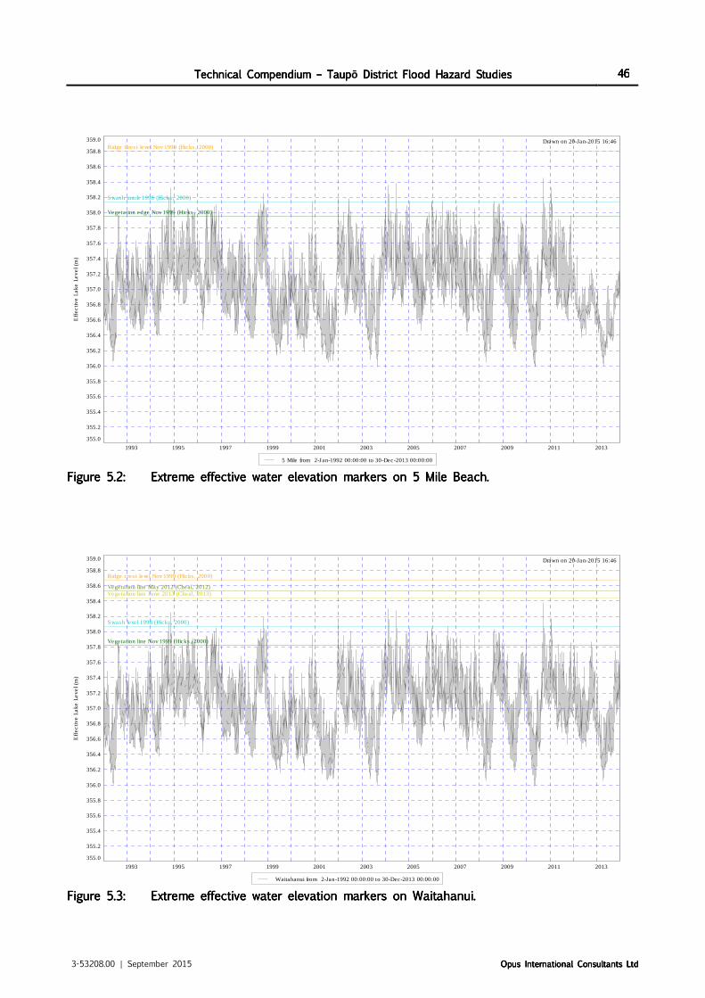
Technical Compendium Technical Compendium Technical Compendium Technical Compendium –––– TaupTaupTaupTaupō District Flood Hazard StudiesDistrict Flood Hazard StudiesDistrict Flood Hazard StudiesDistrict Flood Hazard Studies 46464646
3-53208.00 | September 2015 Opus International Consultants LtdOpus International Consultants LtdOpus International Consultants LtdOpus International Consultants Ltd
Figure Figure Figure Figure 5555....2222:::: Extreme effective water elevation markers on 5 Mile BeachExtreme effective water elevation markers on 5 Mile BeachExtreme effective water elevation markers on 5 Mile BeachExtreme effective water elevation markers on 5 Mile Beach....
Figure Figure Figure Figure 5555....3333:::: Extreme effective water elevation markers on WaitahanuiExtreme effective water elevation markers on WaitahanuiExtreme effective water elevation markers on WaitahanuiExtreme effective water elevation markers on Waitahanui....
1993 1995 1997 1999 2001 2003 2005 2007 2009 2011 2013
355.0
355.2
355.4
355.6
355.8
356.0
356.2
356.4
356.6
356.8
357.0
357.2
357.4
357.6
357.8
358.0
358.2
358.4
358.6
358.8
359.0
Eff
ective L
ake L
evel (m
)
Drawn on 20-Jan-2015 16:46
Swash mark 1998 (Hicks, 2000)
Ridge Crest level Nov 1999 (Hicks, 2000)
Vegetation edge Nov 1999 (Hicks, 2000)
5 Mile from 2-Jan-1992 00:00:00 to 30-Dec-2013 00:00:00
1993 1995 1997 1999 2001 2003 2005 2007 2009 2011 2013
355.0
355.2
355.4
355.6
355.8
356.0
356.2
356.4
356.6
356.8
357.0
357.2
357.4
357.6
357.8
358.0
358.2
358.4
358.6
358.8
359.0
Eff
ective L
ake L
evel (m
)
Drawn on 20-Jan-2015 16:46
Swash level 1998 (Hicks, 2000)
Ridge crest level Nov 1999 (Hicks, 2000)
Vegetation line Nov 1999 (Hicks, 2000)
Vegetation line May 2012 (Cheal, 2012)Vegetation line June 2013 (Cheal, 2013)
Waitahanui from 2-Jan-1992 00:00:00 to 30-Dec-2013 00:00:00

Technical Compendium Technical Compendium Technical Compendium Technical Compendium –––– TaupTaupTaupTaupō District Flood Hazard StudiesDistrict Flood Hazard StudiesDistrict Flood Hazard StudiesDistrict Flood Hazard Studies 47474747
3-53208.00 | September 2015 Opus International Consultants LtdOpus International Consultants LtdOpus International Consultants LtdOpus International Consultants Ltd
Figure Figure Figure Figure 5555....4444:::: Extreme effective water elevation markers on HatepeExtreme effective water elevation markers on HatepeExtreme effective water elevation markers on HatepeExtreme effective water elevation markers on Hatepe....
Figure Figure Figure Figure 5555....5555:::: Extreme effective water elevation markers on Te RangiitaExtreme effective water elevation markers on Te RangiitaExtreme effective water elevation markers on Te RangiitaExtreme effective water elevation markers on Te Rangiita....
1993 1995 1997 1999 2001 2003 2005 2007 2009 2011 2013
355.0
355.2
355.4
355.6
355.8
356.0
356.2
356.4
356.6
356.8
357.0
357.2
357.4
357.6
357.8
358.0
358.2
358.4
358.6
358.8
359.0
Eff
ective L
ake L
evel (m
)
Drawn on 20-Jan-2015 16:46
Swash mark 1998 (Hicks, 2000)
Ridge crest Nov 1999 (Hicks, 2000)
Vegetation line Nov 1999 (Hicks, 2000)
Vegetation line May 2012 (Cheal, 2012)
Vegetaion line July 2013 (Cheal, 2013)
Hatepe from 2-Jan-1992 00:00:00 to 30-Dec-2013 00:00:00
1993 1995 1997 1999 2001 2003 2005 2007 2009 2011 2013
355.0
355.2
355.4
355.6
355.8
356.0
356.2
356.4
356.6
356.8
357.0
357.2
357.4
357.6
357.8
358.0
358.2
358.4
358.6
358.8
359.0
Eff
ective L
ake L
evel (m
)
Drawn on 20-Jan-2015 16:45
Swash mark 1998 (Hicks, 2000)
Ridge crest level Nov 1999 (Hicks, 2000)Vegetation line Nov 1999 (Hicks, 2000)
Te Rangiita from 2-Jan-1992 00:00:00 to 30-Dec-2013 00:00:00

Technical Compendium Technical Compendium Technical Compendium Technical Compendium –––– TaupTaupTaupTaupō District Flood Hazard StudiesDistrict Flood Hazard StudiesDistrict Flood Hazard StudiesDistrict Flood Hazard Studies 48484848
3-53208.00 | September 2015 Opus International Consultants LtdOpus International Consultants LtdOpus International Consultants LtdOpus International Consultants Ltd
Figure Figure Figure Figure 5555....6666:::: Extreme effective water elevation markers on WaihiExtreme effective water elevation markers on WaihiExtreme effective water elevation markers on WaihiExtreme effective water elevation markers on Waihi....
Figure Figure Figure Figure 5555....7777:::: Extreme effective water elevation markers on KuratauExtreme effective water elevation markers on KuratauExtreme effective water elevation markers on KuratauExtreme effective water elevation markers on Kuratau....
1993 1995 1997 1999 2001 2003 2005 2007 2009 2011 2013
355.0
355.2
355.4
355.6
355.8
356.0
356.2
356.4
356.6
356.8
357.0
357.2
357.4
357.6
357.8
358.0
358.2
358.4
358.6
358.8
359.0
Eff
ective L
ake L
evel (m
)
Drawn on 20-Jan-2015 16:43
Swash mark 1998 (Hicks, 2000)Ridge crest level Nov 1999 (Hicks, 2000)
Vegetation line Nov 1999 (Hicks, 2000)
Waihi from 2-Jan-1992 00:00:00 to 30-Dec-2013 00:00:00
1993 1995 1997 1999 2001 2003 2005 2007 2009 2011 2013
355.0
355.2
355.4
355.6
355.8
356.0
356.2
356.4
356.6
356.8
357.0
357.2
357.4
357.6
357.8
358.0
358.2
358.4
358.6
358.8
359.0
Eff
ective L
ake L
evel (m
)
Drawn on 20-Jan-2015 16:44
Swash level 1998 (Hicks, 2000)Ridge crest Nov 1999 (Hicks, 2000)
Vegetation line Nov 1999 (Hicks, 2000)
Vegetation line May 2012 (Cheal, 2012)
Vegetation line May 2013 (Cheal, 2013)
Kuratau from 2-Jan-1992 00:00:00 to 30-Dec-2013 00:00:00

Technical Compendium Technical Compendium Technical Compendium Technical Compendium –––– TaupTaupTaupTaupō District Flood Hazard StudiesDistrict Flood Hazard StudiesDistrict Flood Hazard StudiesDistrict Flood Hazard Studies 49494949
3-53208.00 | September 2015 Opus International Consultants LtdOpus International Consultants LtdOpus International Consultants LtdOpus International Consultants Ltd
Figure Figure Figure Figure 5555....8888:::: Extreme effective Extreme effective Extreme effective Extreme effective water elevation markers on Kinlochwater elevation markers on Kinlochwater elevation markers on Kinlochwater elevation markers on Kinloch....
Figure Figure Figure Figure 5555....9999:::: Extreme effective water elevation markers on Acacia BayExtreme effective water elevation markers on Acacia BayExtreme effective water elevation markers on Acacia BayExtreme effective water elevation markers on Acacia Bay....
1993 1995 1997 1999 2001 2003 2005 2007 2009 2011 2013
355.0
355.2
355.4
355.6
355.8
356.0
356.2
356.4
356.6
356.8
357.0
357.2
357.4
357.6
357.8
358.0
358.2
358.4
358.6
358.8
359.0
Eff
ective L
ake L
evel (m
)
Drawn on 20-Jan-2015 16:44
Swash mark 1998 (Hicks, 2000)Ridge crest level Nov 1999 (Hicks, 2000)Vegetation edge Nov 1999 (Hicks, 2000)
Kinloch from 2-Jan-1992 00:00:00 to 30-Dec-2013 00:00:00
1993 1995 1997 1999 2001 2003 2005 2007 2009 2011 2013
355.0
355.2
355.4
355.6
355.8
356.0
356.2
356.4
356.6
356.8
357.0
357.2
357.4
357.6
357.8
358.0
358.2
358.4
358.6
358.8
359.0
Eff
ective L
ake L
evel (m
)
Drawn on 20-Jan-2015 16:45
Swash mark 1998 (Hicks, 2000)
Ridge crest level Nov 1999 (Hicks, 2000)
Vegetation Edge Nov 1999 (Hicks, 2000)
Acacia Bay from 2-Jan-1992 00:00:00 to 30-Dec-2013 00:00:00

Technical Compendium Technical Compendium Technical Compendium Technical Compendium –––– TaupTaupTaupTaupō District Flood Hazard StudiesDistrict Flood Hazard StudiesDistrict Flood Hazard StudiesDistrict Flood Hazard Studies 50505050
3-53208.00 | September 2015 Opus International Consultants LtdOpus International Consultants LtdOpus International Consultants LtdOpus International Consultants Ltd
5.65.65.65.6 NonNonNonNon----contiguous areas contiguous areas contiguous areas contiguous areas –––– lakelakelakelake floodingfloodingfloodingflooding
Flooding of the shoreline of Lake Taupō as a result of high lake levels was assessed in a
different manner to the river-based flooding. Critical water levels were overlaid on the LiDAR-
derived DTM, and adjusted for any effects of tectonic subsidence. Any areas where the elevation
of the ground is less than the water level were initially indicated as ‘flooded’, and the depth of
flooding derived by subtracting the ground elevation from the water level.
This approach to modelling the flood risk, however, assumes that the high water levels can
actually ‘connect’ to any low lying areas inland from the shore. In some cases this ‘connection’
exists i.e. where there are rivers, streams, drains or culverts. However, in other cases the low-
lying areas inland from the shoreline are separated by relatively impermeable beach ridges,
berms, and road embankments etc. In these situations water in the lake cannot move inland
to these areas despite being at a higher elevation.
Consequently all the areas of flooding adjacent to the lake shore were reviewed. Where a
hydraulic connection could be identified between the lake and areas of flooding these were
mapped as having a flood hazard. However, non-contiguous areas of flooding, where no
apparent hydraulic connection could be identified, were removed from the flood hazard map.
As a result there are some areas of low-lying topography inland from the shoreline of Lake
Taupō which are not shown as having a flood risk resulting from high water levels within the
lake. It should be recognised that these areas are, however, likely to be susceptible to flooding
and impeded drainage during localised rainstorm events.
6666 Differences between wave Differences between wave Differences between wave Differences between wave and river floodand river floodand river floodand river floodinginginging
A key difference between the wave run-up and the river-derived flood modelling is the scale at
which the analysis was undertaken. While the river-derived flood modelling considered a 2m or
5m cell size, the wave run-up analysis considered only 10 typical sites or wave environments
around the shoreline of Lake Taupō. It did not consider small lengths of the shoreline.
Consequently the results of the two kinds of modelling have different resolutions and accuracy.
Overall, there is a relatively high degree of consistency between the modelled effective water
levels (i.e. water levels combined with wave run-up) and various physical indicators of the effect
of these high water levels at the shoreline within the various wave environments. The majority
of the differences appear to be within the range of uncertainty associated with the derivation
of effective water levels. However, some of the differences between modelled and observed
extreme water levels could be attributed to the District-scale nature of the modelling and
differences in the exact location of survey lines and corresponding point from which data were
extracted for comparison.
Despite the consistency between the modelled and observed results it is not possible to apply
the results of the wave run-up analysis at the site-scale. The wave run-up at any particular

Technical Compendium Technical Compendium Technical Compendium Technical Compendium –––– TaupTaupTaupTaupō District Flood Hazard StudiesDistrict Flood Hazard StudiesDistrict Flood Hazard StudiesDistrict Flood Hazard Studies 51515151
3-53208.00 | September 2015 Opus International Consultants LtdOpus International Consultants LtdOpus International Consultants LtdOpus International Consultants Ltd
site can be affected by a wide range of parameters e.g. vegetation, large rocks, protection
works, beach slope and character etc. All of these various parameters were not included in
the wave run-up analysis and cannot be included at the scale necessary for a site-specific
analysis. The cost, scale and logistical constraints of such modelling is beyond the scope and
resources available for a District-scale flood assessment.
Consequently, a different approach is necessary to recognise and accommodate the potential
risk from wave run-up compared to the risk from river-based flooding. The risk from wave run-
up, however, will occur on top of and above, the simple flood risk caused by high water levels
in Lake Taupō.
7777 CCCCombined riskombined riskombined riskombined risk
The various studies provided a holistic assessment of the potential flood risk posed by each of
the tributaries and Lake Taupō. Since the flood risk is generally a function of a number of
variables there is the potential for the elements of risk to cumulate, resulting in an over-
estimation of the actual flood risk.
In the case of river flooding there are three main controls: the peak discharge of the design
event; the potential effect of climate change; and any tectonic deformation over the longer
term. The peak discharge of the design event is the major control on the extent and depth of
any inundation. While climate change might increase the peak discharge by ~20%, the effect
of this on the extent and depth of flooding is generally small. In almost every tributary the
increase in flow resulting from climate change tends to ‘fill in’ those areas within the flood
extent which remained ‘dry’ during the 100-year event. The change in the flood extent was
generally within the grid resolution of the floodplain component of the hydraulic model (i.e. 5m).
Because the floodplains of the various tributaries are ‘large’ relative to the flood discharge, the
change in flood depth is also small. For example, a 1km² floodplain such as that of the
Tongariro River requires 10,000m³ of flood water to raise the level by only 1cm. It would
require 100,000m³ to raise the level by 10cm which is still less than the likely resolution of the
various hydraulic models. Consequently, with respect to the flood hazard posed by the rivers,
the potential effect of taking a cumulative and conservative approach is relatively small, and
within the resolution of the models.
With regard to the risk posed by high water levels in Lake Taupō, there are a number of factors
which affect the flood risk. These include the variability in lake level, seiche, the potential effect
of climate change on periods when inflows exceed the discharge capacity of the Taupō Gates,
and any longer term deformation of the shore. The linear addition of all these variables results
in a 100-year water level only 30cm higher than that estimated from the lake level record
alone. Again, this difference in potential water level, or assessed risk, is likely to be at the
limit of the resolution of the terrain model used in the analysis. About two-thirds of the
additional water level is caused by increased inflows caused by climate change. While this
effect is likely to increase only in the longer term it must be added to the contemporary

Technical Compendium Technical Compendium Technical Compendium Technical Compendium –––– TaupTaupTaupTaupō District Flood Hazard StudiesDistrict Flood Hazard StudiesDistrict Flood Hazard StudiesDistrict Flood Hazard Studies 52525252
3-53208.00 | September 2015 Opus International Consultants LtdOpus International Consultants LtdOpus International Consultants LtdOpus International Consultants Ltd
situation so as to provide a ‘realistic expectation’ of the flood risk towards the end of the
longer term planning framework i.e. 100 years hence.
Obviously there is considerable uncertainty as to the potential effects of climate change over
the longer term. However, by adopting a slightly conservative approach it is possible for the
various flood hazard zones to ‘contract’ over time as more robust information becomes available.
It would be significantly more difficult to ‘expand’ the flood hazard zones in the future once
development had occurred if this was to become necessary.
The inclusion of a tectonic component to the flood risk is also considered reasonable and
realistic. The available information shows that while tectonic deformation around the lake shore
is variable, it tends to be relatively consistent at specific locations i.e. either uplift or subsidence.
Consequently it is highly likely that the relative elevation of the ground will change over the
longer term planning time-frame. It is considered appropriate therefore that this element of the
flood risk is added linearly to those other elements affecting the overall flood risk.
Obviously the two principal components of the overall risk of high effective water levels in Lake
Taupō are the relative level of the lake and the waves. The approach taken for deriving the
frequency and magnitude of these combined factors on water levels is considered robust. While
the two elements of risk are combined, they are essentially combined in a ‘Monte Carlo’ fashion
by modelling the combination of the two random variables over time and then assessing the
frequency and magnitude of the resulting effective water level. Again, this approach is considered
reasonable when assessing the potential risk from higher effective water levels over the longer
term.
8888 PurposePurposePurposePurpose
The purpose of the various flood studies was to provide a District-scale assessment of the
potential flood risk over the longer term. The studies were never intended to provide robust
flood risk assessments at the level of individual sites or building platforms. In effect, the studies
were developed largely as a screening tool to identify those areas where flood risk is not a
consideration, and those where some further investigation may be warranted. The uncertainty
inherent in both flood modelling of extreme design events, and a District-scale assessment,
mean that the resulting flood maps should not be regarded as ‘definitive’. While the maps are
robust, given the various assumptions and the contemporary situation, should either of these
change then so too might the flood hazard maps.
It is suggested that the flood hazard maps therefore provide guidance as to what level of
planning control might be appropriate, rather than restricting or denying specific activities. The
maps also indicate where detailed, site-specific studies, might be required before any major
capital works are undertaken.
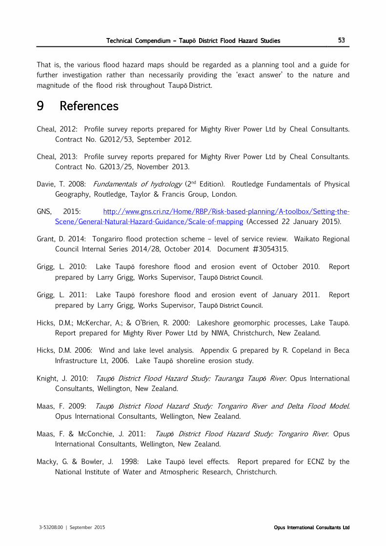
Technical Compendium Technical Compendium Technical Compendium Technical Compendium –––– TaupTaupTaupTaupō District Flood Hazard StudiesDistrict Flood Hazard StudiesDistrict Flood Hazard StudiesDistrict Flood Hazard Studies 53535353
3-53208.00 | September 2015 Opus International Consultants LtdOpus International Consultants LtdOpus International Consultants LtdOpus International Consultants Ltd
That is, the various flood hazard maps should be regarded as a planning tool and a guide for
further investigation rather than necessarily providing the ‘exact answer’ to the nature and
magnitude of the flood risk throughout Taupō District.
9999 ReferencesReferencesReferencesReferences
Cheal, 2012: Profile survey reports prepared for Mighty River Power Ltd by Cheal Consultants.
Contract No. G2012/53, September 2012.
Cheal, 2013: Profile survey reports prepared for Mighty River Power Ltd by Cheal Consultants.
Contract No. G2013/25, November 2013.
Davie, T. 2008: Fundamentals of hydrology (2nd Edition). Routledge Fundamentals of Physical
Geography, Routledge, Taylor & Francis Group, London.
GNS, 2015: http://www.gns.cri.nz/Home/RBP/Risk-based-planning/A-toolbox/Setting-the-
Scene/General-Natural-Hazard-Guidance/Scale-of-mapping (Accessed 22 January 2015).
Grant, D. 2014: Tongariro flood protection scheme – level of service review. Waikato Regional
Council Internal Series 2014/28, October 2014. Document #3054315.
Grigg, L. 2010: Lake Taupō foreshore flood and erosion event of October 2010. Report
prepared by Larry Grigg, Works Supervisor, Taupō District Council.
Grigg, L. 2011: Lake Taupō foreshore flood and erosion event of January 2011. Report
prepared by Larry Grigg, Works Supervisor, Taupō District Council.
Hicks, D.M.; McKerchar, A.; & O’Brien, R. 2000: Lakeshore geomorphic processes, Lake Taupō.
Report prepared for Mighty River Power Ltd by NIWA, Christchurch, New Zealand.
Hicks, D.M. 2006: Wind and lake level analysis. Appendix G prepared by R. Copeland in Beca
Infrastructure Lt, 2006. Lake Taupō shoreline erosion study.
Knight, J. 2010: Taupō District Flood Hazard Study: Tauranga Taupō River. Opus International
Consultants, Wellington, New Zealand.
Maas, F. 2009: Taupō District Flood Hazard Study: Tongariro River and Delta Flood Model.
Opus International Consultants, Wellington, New Zealand.
Maas, F. & McConchie, J. 2011: Taupō District Flood Hazard Study: Tongariro River. Opus
International Consultants, Wellington, New Zealand.
Macky, G. & Bowler, J. 1998: Lake Taupō level effects. Report prepared for ECNZ by the
National Institute of Water and Atmospheric Research, Christchurch.

Technical Compendium Technical Compendium Technical Compendium Technical Compendium –––– TaupTaupTaupTaupō District Flood Hazard StudiesDistrict Flood Hazard StudiesDistrict Flood Hazard StudiesDistrict Flood Hazard Studies 54545454
3-53208.00 | September 2015 Opus International Consultants LtdOpus International Consultants LtdOpus International Consultants LtdOpus International Consultants Ltd
McKerchar, A.I. & Pearson, C.P. 1989: Flood frequency in New Zealand. Publication No. 20,
Hydrology Centre, Division of Water Sciences, Department of Scientific and Industrial
Research, Christchurch, New Zealand.
Opus, 2008: Taupō District Flood Hazard Study – Stage 1: Lake Taupō Foreshore. Report
prepared for Environment Waikato and Taupō District Council by Opus International
Consultants, March 2008.
Paine, S. & Smith, H. 2012a: Taupō District Flood Hazard Study: Hinemaiaia River. Opus
International Consultants, Wellington, New Zealand.
Paine, S. & Smith, H. 2012b: Taupō District Flood Hazard Study: Tokaanu Stream. Opus
International Consultants, Wellington, New Zealand.
Paine, S. & Smith, H. 2012c: Taupō District Flood Hazard Study: Whareroa Stream. Opus
International Consultants, Wellington, New Zealand.
Smith, H., Paine, S. & Ward, H. 2011: Taupō District Flood Hazard Study: Kuratau River. Opus
International Consultants, Wellington, New Zealand.
T&T, 2004: Tongariro River model update, Tonkin and Taylor, August 2004.
WRC, 2015: http://www.waikatoregion.govt.nz/Services/Regional-services/Regional-hazards-and-
emergency-management/River-flooding/Broadscale-information/ (Accessed 22 January
2015).

Technical Compendium Technical Compendium Technical Compendium Technical Compendium –––– TaupTaupTaupTaupō District Flood Hazard StudiesDistrict Flood Hazard StudiesDistrict Flood Hazard StudiesDistrict Flood Hazard Studies 55555555
3-53208.00 | September 2015 Opus International Consultants LtdOpus International Consultants LtdOpus International Consultants LtdOpus International Consultants Ltd

Opus International Consultants LtdOpus International Consultants LtdOpus International Consultants LtdOpus International Consultants Ltd
L10, Majestic Centre, 100 Willis St
PO Box 12 003, Thorndon, Wellington 6144
New Zealand
t: +64 4 471 7000
f: +64 4 499 3699
w: www.opus.co.nz