Embed Size (px)
Citation preview
ICEAA 2016 Bristol – TRN 07
v1.2
© 2002-2013 ICEAA. All rights reserved.
Unit III - Module 10 1
Probability and Statistics
Mathematical underpinnings of cost estimating
“God does not play dice with the cosmos.” -Albert Einstein “Do not presume to tell God what to do.” -Niels Bohr
http://en.wikiquote.org/wiki/Quantum_mechanics
v1.2
© 2002-2013 ICEAA. All rights reserved.
Acknowledgments• ICEAA is indebted to TASC, Inc., for the
development and maintenance of theCost Estimating Body of Knowledge (CEBoK®)– ICEAA is also indebted to Technomics, Inc., for the
independent review and maintenance of CEBoK®
• ICEAA is also indebted to the following individuals who have made significant contributions to the development, review, and maintenance of CostPROF and CEBoK ®
• Module 10 Probability and Statistics– Lead authors: Megan E. Dameron, Christopher J. Leonetti, Casey D. Trail
– Assistant authors: Jessica R. Summerville, Jennifer K. Murrill, Sarah E. Grinnell
– Senior reviewers: Richard L. Coleman, Kevin Cincotta, Fred K. Blackburn
– Reviewers: Robyn Kane, Matthew J. Pitlyk, Maureen L. Tedford
– Managing editor: Peter J. Braxton
2Unit III - Module 10

ICEAA 2016 Bristol – TRN 07
v1.2
© 2002-2013 ICEAA. All rights reserved.
Unit III - Module 10 3
Unit IndexUnit I – Cost EstimatingUnit II – Cost Analysis TechniquesUnit III – Analytical Methods
6. Basic Data Analysis Principles7. Learning Curve Analysis8. Regression Analysis9. Cost and Schedule Risk Analysis10.Probability and Statistics
Unit IV – Specialized CostingUnit V – Management Applications
v1.2
© 2002-2013 ICEAA. All rights reserved.
Unit III - Module 10 4
Statistics
Prob/Stat Overview• Key Ideas
– Probability and Statistics as “Flipsides”
– Central Tendency and Dispersion– The Bell Curve
• Normal (Gaussian) Distribution and the CLT
– Inference
• Practical Applications– Descriptive Statistics
• Mean, Median, Mode, CV
– CER Development• t, F, R2, CI, PI
– Modeling Uncertainty and Risk• Normal, Triangular, Lognormal
• Analytical Constructs– Counting and Fractions
• Combinations and Permutations
• Pascal’s Triangle
– Distributions and Calculus• pdfs and cdfs
• Limits
• (Maximum Likelihood) Estimators
– Hypothesis Testing• Test statistic, critical values, significance
9
8
6
• Related Topics– Stochastic Processes
• Markov Chains
• Queueing Theory
– Simulation• Discrete Event
• Continuous
– Data Analysis
– Regression Analysis
– Design of Experiments
Probability
ICEAA 2016 Bristol – TRN 07
v1.2
© 2002-2013 ICEAA. All rights reserved.
Unit III - Module 10 5
2 3 4 5 6 7 8 9 10 11 12
2 3 4 5 6 7 8 9 10 11 12
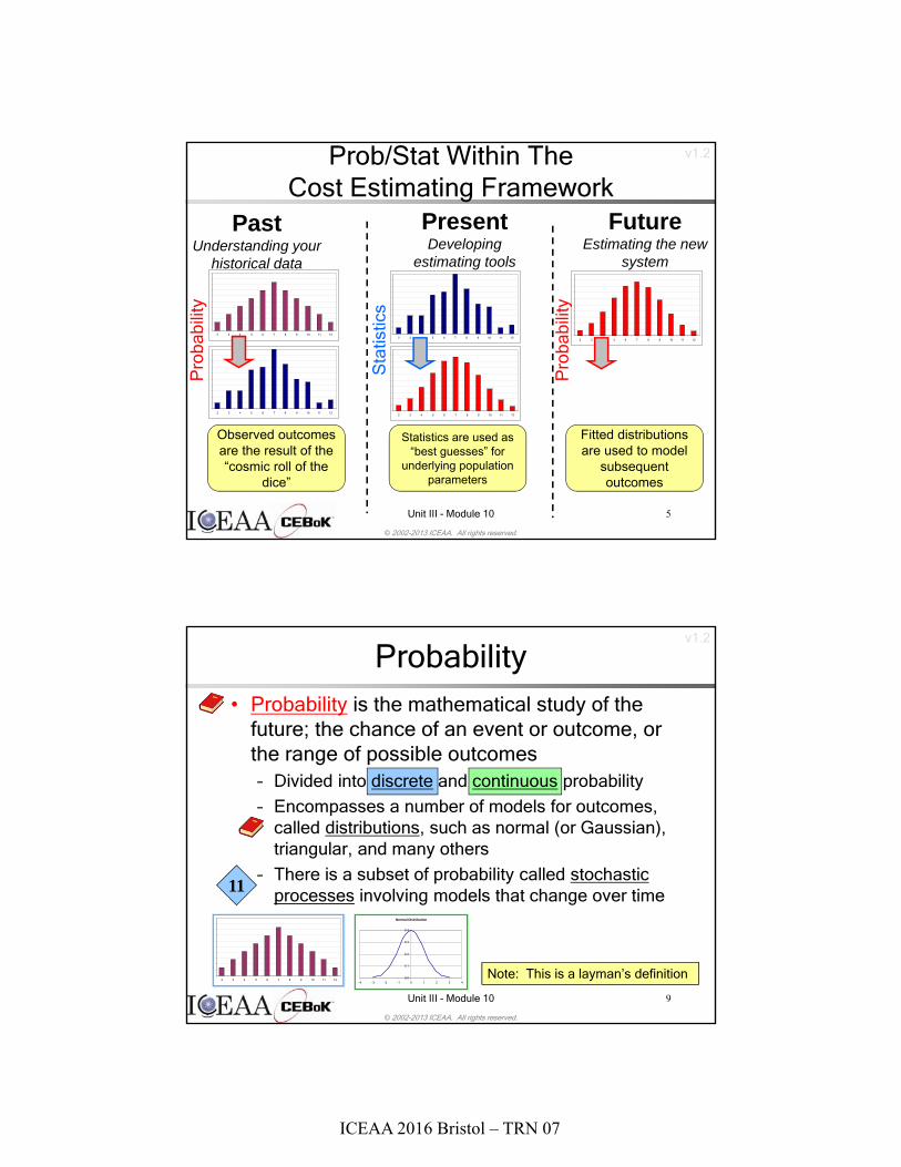
Prob/Stat Within TheCost Estimating Framework
PastUnderstanding your
historical data
PresentDeveloping
estimating tools
FutureEstimating the new
system
Observed outcomes are the result of the “cosmic roll of the
dice”
Statistics are used as “best guesses” for
underlying population parameters
Fitted distributions are used to model
subsequent outcomes
2 3 4 5 6 7 8 9 10 11 12
2 3 4 5 6 7 8 9 10 11 122 3 4 5 6 7 8 9 10 11 12
Pro
babi
lity
Pro
babi
lity
Sta
tistic
s
v1.2
© 2002-2013 ICEAA. All rights reserved.
Unit III - Module 10 9
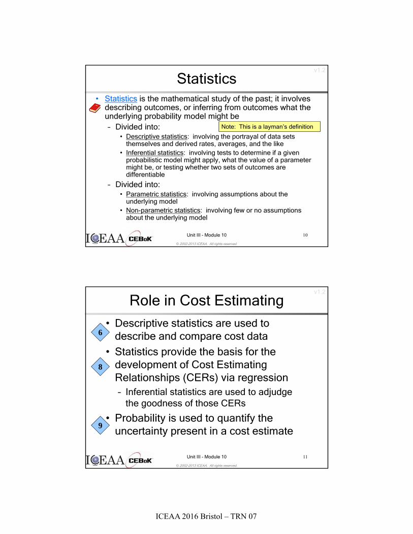
• Probability is the mathematical study of the future; the chance of an event or outcome, or the range of possible outcomes– Divided into discrete and continuous probability
– Encompasses a number of models for outcomes, called distributions, such as normal (or Gaussian), triangular, and many others
– There is a subset of probability called stochastic processes involving models that change over time
Probability
Note: This is a layman’s definition
11
Normal Distribution
0.0
0.1
0.2
0.3
0.4
-4 -3 -2 -1 0 1 2 3 42 3 4 5 6 7 8 9 10 11 12
ICEAA 2016 Bristol – TRN 07
v1.2
© 2002-2013 ICEAA. All rights reserved.
Unit III - Module 10 10
Statistics• Statistics is the mathematical study of the past; it involves
describing outcomes, or inferring from outcomes what the underlying probability model might be– Divided into:
• Descriptive statistics: involving the portrayal of data sets themselves and derived rates, averages, and the like
• Inferential statistics: involving tests to determine if a given probabilistic model might apply, what the value of a parameter might be, or testing whether two sets of outcomes are differentiable
– Divided into:• Parametric statistics: involving assumptions about the
underlying model• Non-parametric statistics: involving few or no assumptions
about the underlying model
Note: This is a layman’s definition
v1.2
© 2002-2013 ICEAA. All rights reserved.
Unit III - Module 10 11
Role in Cost Estimating
• Descriptive statistics are used to describe and compare cost data
• Statistics provide the basis for the development of Cost Estimating Relationships (CERs) via regression– Inferential statistics are used to adjudge
the goodness of those CERs
• Probability is used to quantify the uncertainty present in a cost estimate
9
8
6

ICEAA 2016 Bristol – TRN 07
v1.2
© 2002-2013 ICEAA. All rights reserved.
Unit III - Module 10 12
Definitions – Population / Sample• A population consists of all members of a particular
group, e.g., all (metaphysically possible) US Navy destroyers
• A sample is a subset of the population, e.g., DDG 51 and DD 963 classes
Population
Sample
Parameters
Statistics
x, s2
Statistics are used to draw conclusions about the population from outcomes in the past
Probability uses population parameters to describe future outcomes that are subject to
chance
v1.2
© 2002-2013 ICEAA. All rights reserved.
Unit III - Module 10 13
Definitions – Random Variables
• A random variable takes on values that represent outcomes in the sample space– It cannot be fully controlled or exactly predicted
• Discrete vs. Continuous– A set is discrete if it consists of a finite or
countably infinite number of values• e.g., number of circuits, number of test failures• e.g., {1,2,3, …} – the random variable can only have a
positive integer (natural number) value
– A set is continuous if it consists of an interval of real numbers (finite or infinite length)
• e.g., time, height, weight• e.g., [-3,3] – the random variable can take on any value in
this interval

ICEAA 2016 Bristol – TRN 07
v1.2
© 2002-2013 ICEAA. All rights reserved.
Unit III - Module 10 14
Definitions – pmf• Probability Mass Function
(pmf)– The probability that the
discrete random variable will take a value equal to a is the height of the bar at a.
– The pmf accounts for all possible outcomes of the distribution
• The sum of heights of all bars is 1.
)(afaXP XPossible outcome of Random Variable
Probability Mass Function
The probability of a given outcome is the height of the
corresponding histogram bar.
Xf
NEW!
Tip: Discrete distributions are the exception, not the rule, in cost estimating
v1.2
© 2002-2013 ICEAA. All rights reserved.
Unit III - Module 10 15
Definitions – pdf• Probability Density
Function (pdf)– The total area under the
curve is 1• The probability that the
random variable takes on some value in the range is 1 (100%)
– The probability that the continuous random variable will take a value between aand b is the area under the curve between a and b
The probability that this random variable is between a=5 and b=10 is equal to the
shaded area (40%)
dxxpbXaPb
a
ICEAA 2016 Bristol – TRN 07
v1.2
© 2002-2013 ICEAA. All rights reserved.
Cumulative Density Function
0.00
0.20
0.40
0.60
0.80
1.00
0.0 5.0 10.0 15.0 20.0 25.0
Possible Outcomes of Random Variable
Cumulative Distribution Function
Unit III - Module 10 16
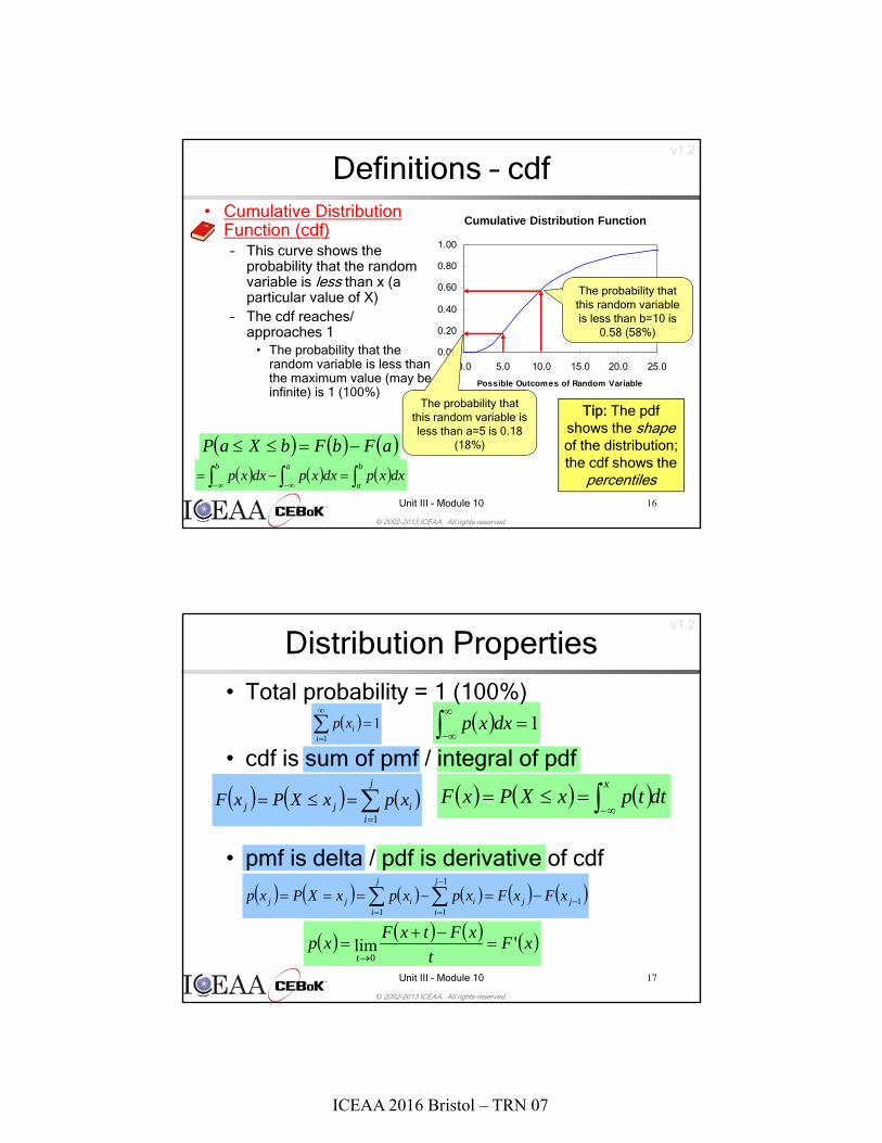
Definitions – cdf• Cumulative Distribution
Function (cdf)– This curve shows the
probability that the random variable is less than x (a particular value of X)
– The cdf reaches/ approaches 1
• The probability that the random variable is less than the maximum value (may be infinite) is 1 (100%)
The probability that this random variable is less than b=10 is
0.58 (58%)
The probability that this random variable is less than a=5 is 0.18
(18%)
b
a
abdxxpdxxpdxxp
aFbFbXaP
Tip: The pdf shows the shapeof the distribution; the cdf shows the
percentiles
v1.2
© 2002-2013 ICEAA. All rights reserved.
Unit III - Module 10 17
Distribution Properties
11
iixp 1
dxxp
j
iijj xpxXPxF
1
dttpxXPxFx
1
1
11
jj
j
ii
j
iijj xFxFxpxpxXPxp
xFt
xFtxFxp
t'lim
0
• Total probability = 1 (100%)
• cdf is sum of pmf / integral of pdf
• pmf is delta / pdf is derivative of cdf

ICEAA 2016 Bristol – TRN 07
v1.2
© 2002-2013 ICEAA. All rights reserved.
Unit III - Module 10 19
Measures of Central Tendency
Where is the “center” of the distribution?
v1.2
© 2002-2013 ICEAA. All rights reserved.
Unit III - Module 10 20
Mean• The expected value of a distribution (population mean), is
calculated as the sum (integral) of a random variable’s possible values multiplied by the probability that it takes on those values
ii xpxXE dxxxpXE 7
36
112
36
211
36
67
36
23
36
12
XE
dxex
dxedxex
XExxx
2
2
2
2
2
2
222
22
1
2
2
2
2
2
x
e
6 1
ICEAA 2016 Bristol – TRN 07
v1.2
© 2002-2013 ICEAA. All rights reserved.
Unit III - Module 10 21
6
Median• The median of a distribution is the value that exactly
divides the distribution (pdf) into equal halves (middle value or average of two middle values); “robust” to extreme values
12
1
2
1 2
2
2
2
22
dxedxe
xx
2
1
2
1
2
1 2
2
2
2
22
dxedxe
xx
The median of a Normal distribution – as with any symmetric distribution with finite mean – is its mean
m
2
1
mxi
i
xp 2
1
mxi
i
xp 2
1
dxxpm
2
1
dxxpm
2
1
mxi
i
xp 2
1
mxi
i
xp
Note that the median may not be in the distribution
2
2
1
dxxp
m
2
1
dxxp
m
v1.2
© 2002-2013 ICEAA. All rights reserved.
Unit III - Module 10 22
Lognormal Distribution
0
0.01
0.02
0.03
0.04
0.05
0.06
0 5 10 15 20 25 30 35
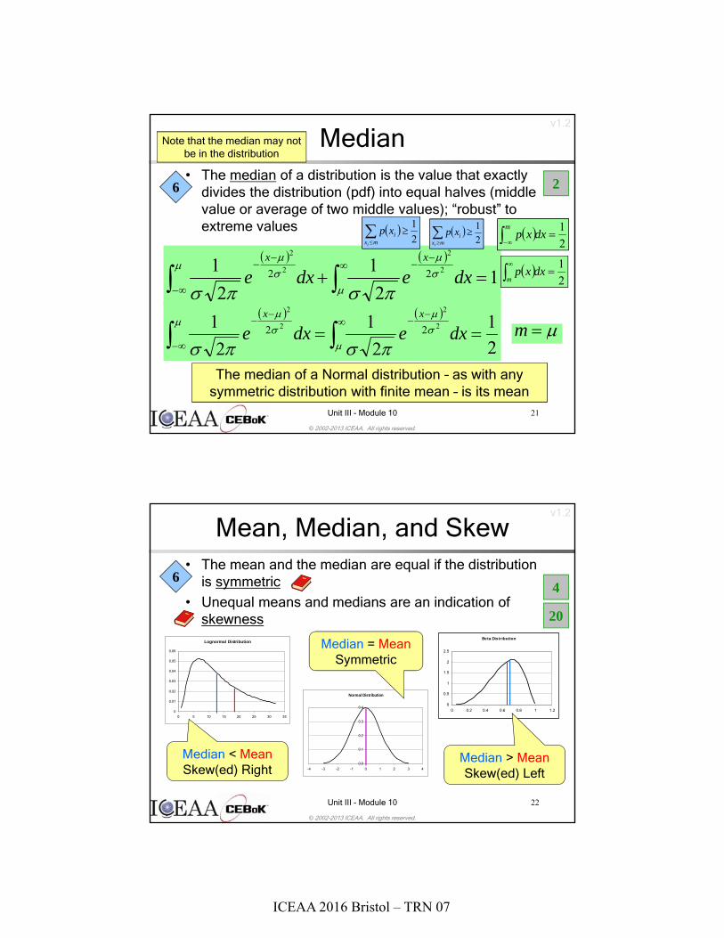
Mean, Median, and Skew• The mean and the median are equal if the distribution
is symmetric
• Unequal means and medians are an indication of skewness
Median < Mean Skew(ed) Right
Normal Distribution
0.0
0.1
0.2
0.3
0.4
-4 -3 -2 -1 0 1 2 3 4
Median = MeanSymmetric
Beta Distribution
0
0.5
1
1.5
2
2.5
0 0.2 0.4 0.6 0.8 1 1.2
Median > Mean Skew(ed) Left
4
20
6
ICEAA 2016 Bristol – TRN 07
v1.2
© 2002-2013 ICEAA. All rights reserved.
Unit III - Module 10 23
6
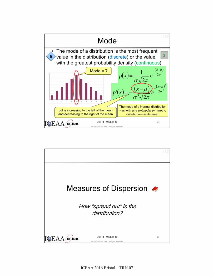
Mode• The mode of a distribution is the most frequent
value in the distribution (discrete) or the value with the greatest probability density (continuous)
2 3 4 5 6 7 8 9 10 11 12
Mode = 7
2
2
2
2
1
x
exp
2
2
23 2
'
x
ex
xp
pdf is increasing to the left of the mean and decreasing to the right of the mean
The mode of a Normal distribution – as with any unimodal symmetric
distribution – is its mean
3
v1.2
© 2002-2013 ICEAA. All rights reserved.
Unit III - Module 10 24
Measures of Dispersion
How “spread out” is the distribution?

ICEAA 2016 Bristol – TRN 07
v1.2
© 2002-2013 ICEAA. All rights reserved.
Unit III - Module 10 25
Variance / Standard Deviation• The variance of a distribution is the measure of the “spread” of the
distribution about its mean – the second “moment”
ii xpxXEXVar 22
dxxpxXEXVar 22
38.56
35
36
125
36
216
36
60
36
216
36
125
XVar
22222
22
2
2
2
2
2
2
1
22
dxeex
dxex
XVarxxx
std dev of about 2.42
The variance of a distribution is the square of , its standard deviation
6
v1.2
© 2002-2013 ICEAA. All rights reserved.
Unit III - Module 10 27
Coefficient of Variation• The Coefficient of Variation (CV) expresses the standard
deviation as a percent of the mean
• Large CVs indicate that the mean is a poor representation of the distribution– Specify distribution using complete set of parameters, if possible
– Include other parameters, such as variance
• CV is invariant to scaling.– e.g., CV{1,2,3}=CV{100,200,300}
• Not to be confused with the CV regression statistic
Tip: Low CV indicates less
dispersion, i.e., a tighter distribution
5
CV
6
6
8
ICEAA 2016 Bristol – TRN 07
v1.2
© 2002-2013 ICEAA. All rights reserved.
Unit III - Module 10 28
0
0.05
0.1
0.15
0.2
0.25
0.3
-30 -20 -10 0 10 20 30
Lower CV
Higher CV
Dispersion and CV
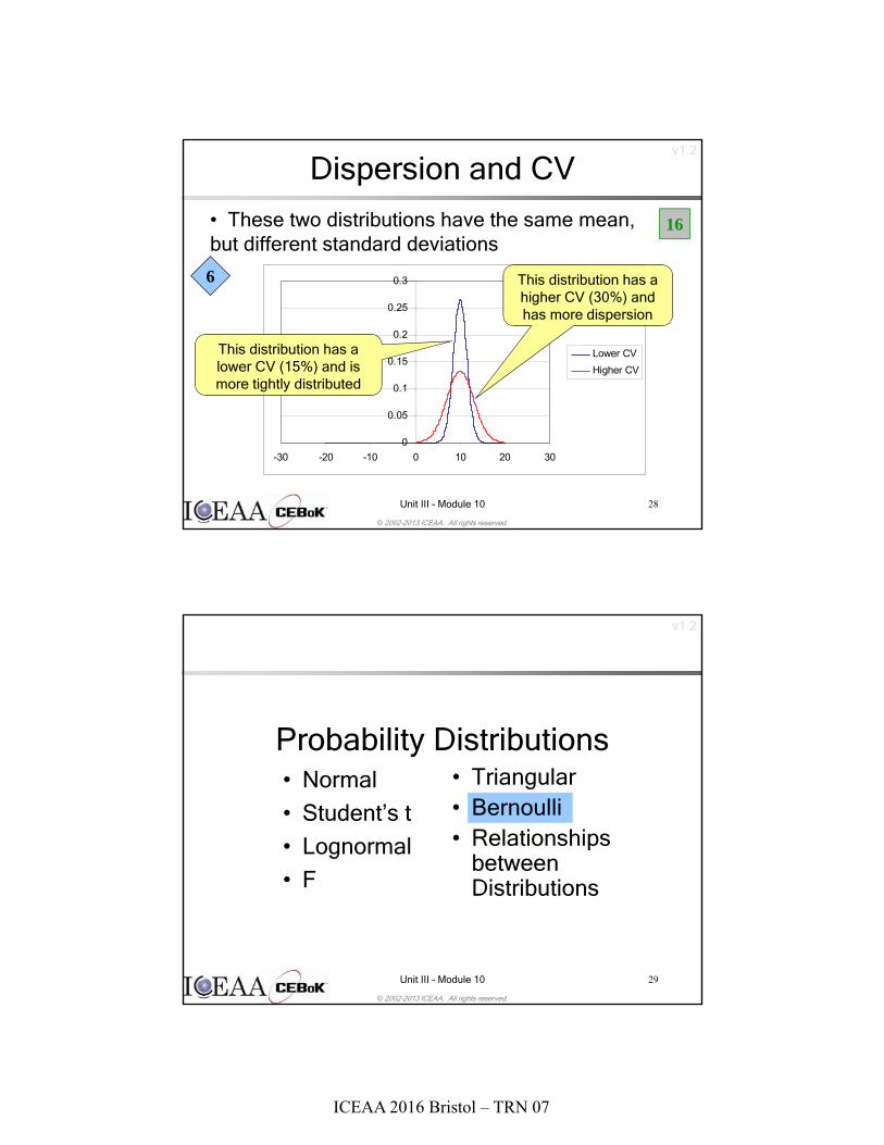
• These two distributions have the same mean, but different standard deviations
This distribution has a lower CV (15%) and is more tightly distributed
This distribution has a higher CV (30%) and has more dispersion
16
6
v1.2
© 2002-2013 ICEAA. All rights reserved.
Unit III - Module 10 29
Probability Distributions• Normal
• Student’s t
• Lognormal
• F
• Triangular• Bernoulli• Relationships
between Distributions
ICEAA 2016 Bristol – TRN 07
v1.2
© 2002-2013 ICEAA. All rights reserved.
Unit III - Module 10 30
Normal (Gaussian)
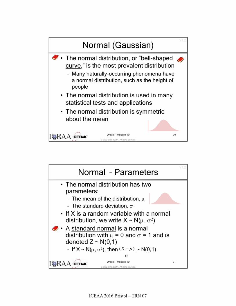
• The normal distribution, or “bell-shaped curve,” is the most prevalent distribution– Many naturally-occurring phenomena have
a normal distribution, such as the height of people
• The normal distribution is used in many statistical tests and applications
• The normal distribution is symmetric about the mean
v1.2
© 2002-2013 ICEAA. All rights reserved.
Unit III - Module 10 31
Normal – Parameters• The normal distribution has two
parameters:– The mean of the distribution, – The standard deviation,
• If X is a random variable with a normal distribution, we write X ~ N(, )
• A standard normal is a normal distribution with = 0 and = 1 and is denoted Z ~ N(0,1)– If X ~ N(, ), then ~ N(0,1)
)( X
ICEAA 2016 Bristol – TRN 07
v1.2
© 2002-2013 ICEAA. All rights reserved.
Unit III - Module 10 32
Normal – pdf
Normal Distribution
0.0
0.1
0.2
0.3
0.4
-4 -3 -2 -1 0 1 2 3 4
= 0
= 1
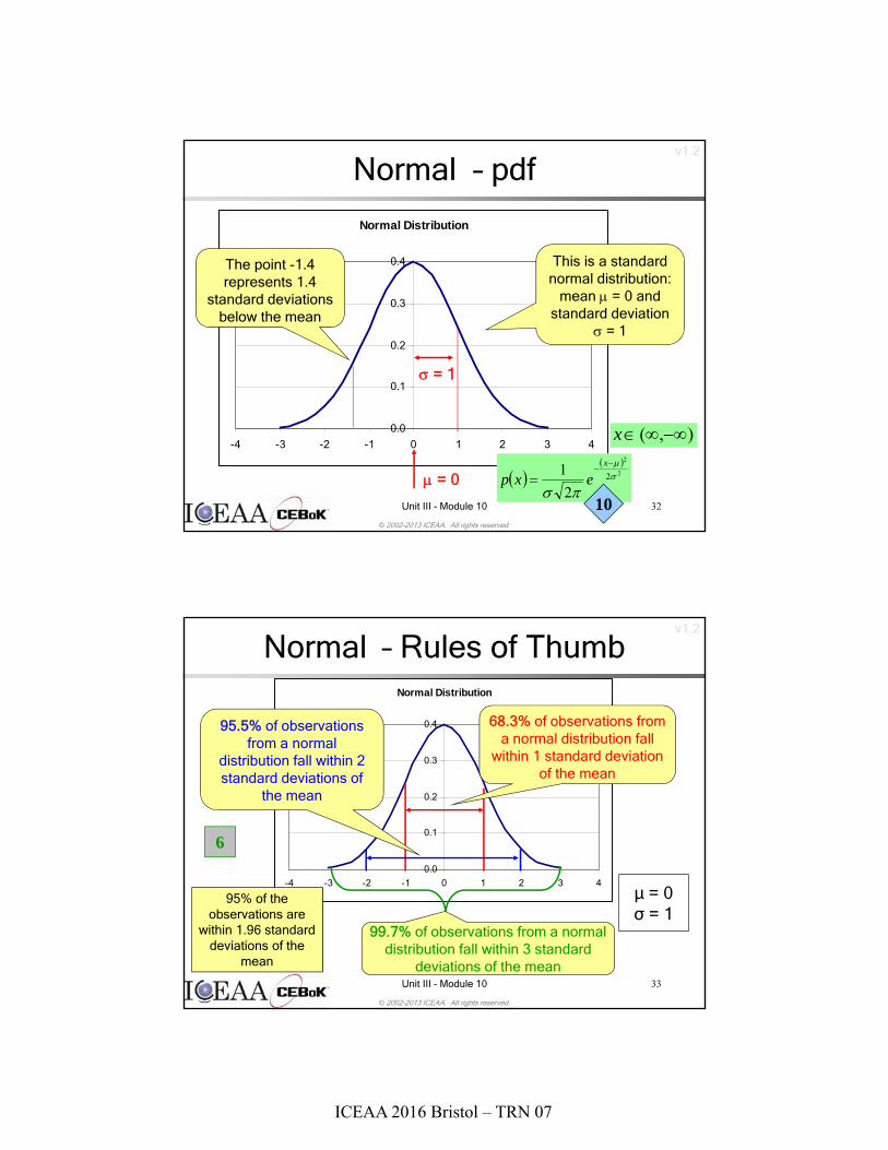
This is a standard normal distribution:
mean = 0 and standard deviation
= 1
The point -1.4 represents 1.4
standard deviations below the mean
2
2
2
2
1
x
exp
10
),( x
v1.2
© 2002-2013 ICEAA. All rights reserved.
Unit III - Module 10 33
Normal – Rules of ThumbNormal Distribution
0.0
0.1
0.2
0.3
0.4
-4 -3 -2 -1 0 1 2 3 4
68.3% of observations from a normal distribution fall
within 1 standard deviation of the mean
95.5% of observations from a normal
distribution fall within 2 standard deviations of
the mean
99.7% of observations from a normal distribution fall within 3 standard
deviations of the mean
μ = 0σ = 1
6
95% of the observations are
within 1.96 standard deviations of the
mean

ICEAA 2016 Bristol – TRN 07
v1.2
© 2002-2013 ICEAA. All rights reserved.
Unit III - Module 10 34
Central Limit Theorem (CLT)• The sum of a large number of independent,
identically distributed (iid) random variables from a population with finite mean and standard deviation approaches a normal distribution– Sample size required depends on the parent
distribution, but as a rule of thumb, distributions approach normal by n = 30
• Correlation: As long as the sum is not dominated by a few large, highly correlated elements, the CLT will still hold
Normality of Work Breakdown Structures, M. Dameron, J. Summerville, R. Coleman, N.St. Louis, Joint ISPA/SCEA Conference, June 2001.
7
v1.2
© 2002-2013 ICEAA. All rights reserved.
Unit III - Module 10 35
CLT – Example• The graph below shows 3 triangular
distributions and the sum of the 3 triangles
Sum of Triangles
.000
.038
.077
.115
.153
0.00 5.00 10.00 15.00 20.00
Normal Distribution(15.43, 1.52)
Triangle 1
Triangle 2
Triangle 3
Sum of 3 Triangles
Overlay Chart
The sum of three independent
triangular distributions
tests as being normally
distributed
“Normality of Work Breakdown Structures,” M. Dameron, J. Summerville, R. Coleman, N. St. Louis, Joint ISPA/SCEA Conference, June 2001.
ICEAA 2016 Bristol – TRN 07
v1.2
© 2002-2013 ICEAA. All rights reserved.
Unit III - Module 10 36
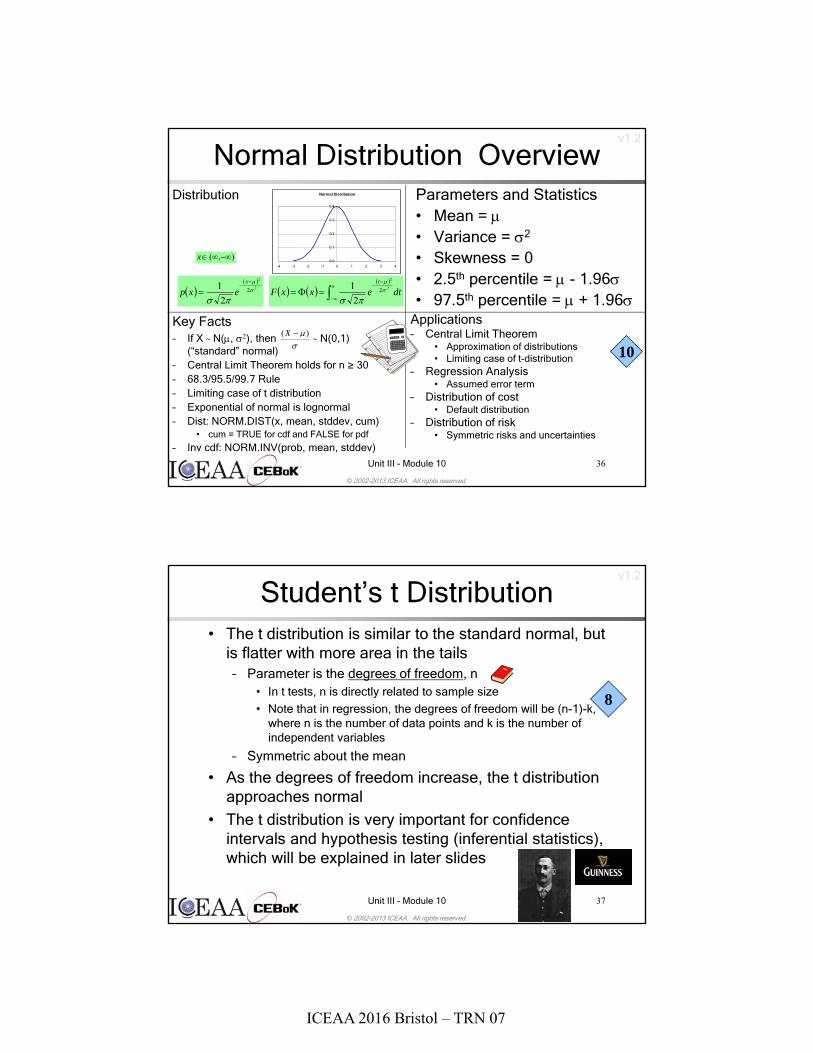
Normal Distribution OverviewDistribution Parameters and Statistics
• Mean = • Variance = 2
• Skewness = 0• 2.5th percentile = - 1.96• 97.5th percentile = + 1.96
Key Facts– If X ~ N(, ), then ~ N(0,1)
(“standard” normal)– Central Limit Theorem holds for n ≥ 30 – 68.3/95.5/99.7 Rule– Limiting case of t distribution– Exponential of normal is lognormal– Dist: NORM.DIST(x, mean, stddev, cum)
• cum = TRUE for cdf and FALSE for pdf
– Inv cdf: NORM.INV(prob, mean, stddev)
Applications– Central Limit Theorem
• Approximation of distributions• Limiting case of t-distribution
– Regression Analysis• Assumed error term
– Distribution of cost• Default distribution
– Distribution of risk• Symmetric risks and uncertainties
)( X
Normal Distribution
0.0
0.1
0.2
0.3
0.4
-4 -3 -2 -1 0 1 2 3 4
2
2
2
2
1
x
exp
x
t
dtexxF2
2
2
2
1
),( x
10
v1.2
© 2002-2013 ICEAA. All rights reserved.
Unit III - Module 10 37
Student’s t Distribution• The t distribution is similar to the standard normal, but
is flatter with more area in the tails– Parameter is the degrees of freedom, n
• In t tests, n is directly related to sample size
• Note that in regression, the degrees of freedom will be (n-1)-k, where n is the number of data points and k is the number of independent variables
– Symmetric about the mean
• As the degrees of freedom increase, the t distribution approaches normal
• The t distribution is very important for confidence intervals and hypothesis testing (inferential statistics), which will be explained in later slides
8
ICEAA 2016 Bristol – TRN 07
v1.2
© 2002-2013 ICEAA. All rights reserved.
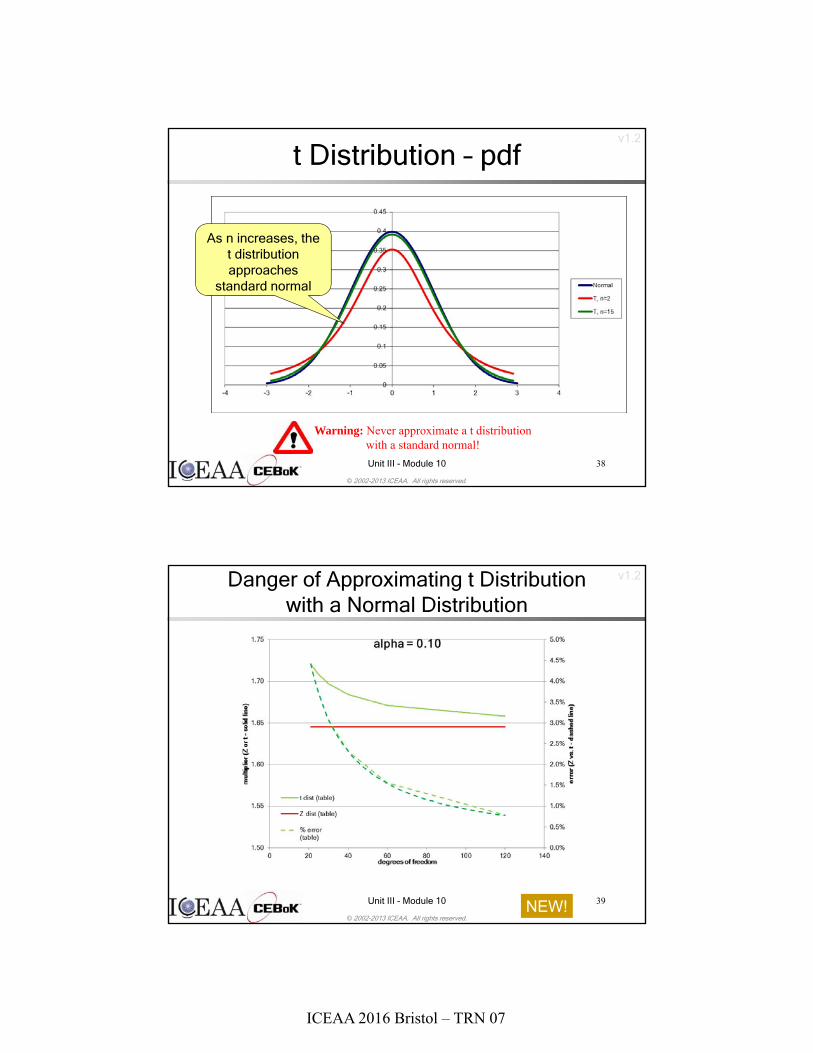
As n increases, the t distribution approaches
standard normal
Unit III - Module 10 38
t Distribution – pdf
Warning: Never approximate a t distribution with a standard normal!
v1.2
© 2002-2013 ICEAA. All rights reserved.
Danger of Approximating t Distribution with a Normal Distribution
Unit III - Module 10 39NEW!

ICEAA 2016 Bristol – TRN 07
v1.2
© 2002-2013 ICEAA. All rights reserved.
Unit III - Module 10 40
t Distribution OverviewDistribution Parameters and Statistics
• Degrees of freedom = n• Mean = 0• Variance = • Skewness = 0
Key Facts– As n approaches infinity, the t distribution
approaches Standard Normal– The t is distributed as – Excel
• cdf = T.DIST(x, n, tails)– Default is left-hand tail, use .2T for two
tails, .RT for right-hand tail
• Inv cdf = T.INV(prob, n)
Applications
– Confidence Intervals• Mean of Normal variates
– Regression Analysis• Significance of individual coefficients
– Hypothesis Testing
2/)1(2 )]/(1)[2/(
]2/)1[(
nnxnn
nxp
2n
n),( x
nn
Nt
/)(
)1,0(
0
0.05
0.1
0.15
0.2
0.25
0.3
0.35
0.4
-4 -3 -2 -1 0 1 2 3 4
v1.2
© 2002-2013 ICEAA. All rights reserved.
Unit III - Module 10 41
Lognormal Distribution• The lognormal distribution :
– Formed by raising e to the power of (“exponentiating”) a normal random variable. is lognormal.
– Not the log of a normal. Rather, a variable is lognormal if its (natural) log is normal. Also, the (natural) log of a lognormal is normal.
– The mean of the related normal distribution, – The standard deviation of the related normal distribution,
Lognormal Distribution
0
0.01
0.02
0.03
0.04
0.05
0.06
0 5 10 15 20 25 30 35
Tip: If the distribution of X
is lognormal, then the natural log (ln) of X is
normally distributed.
The lognormal
distribution is skewed right
YeNY ),(~ 2
ICEAA 2016 Bristol – TRN 07
v1.2
© 2002-2013 ICEAA. All rights reserved.
Unit III - Module 10 42
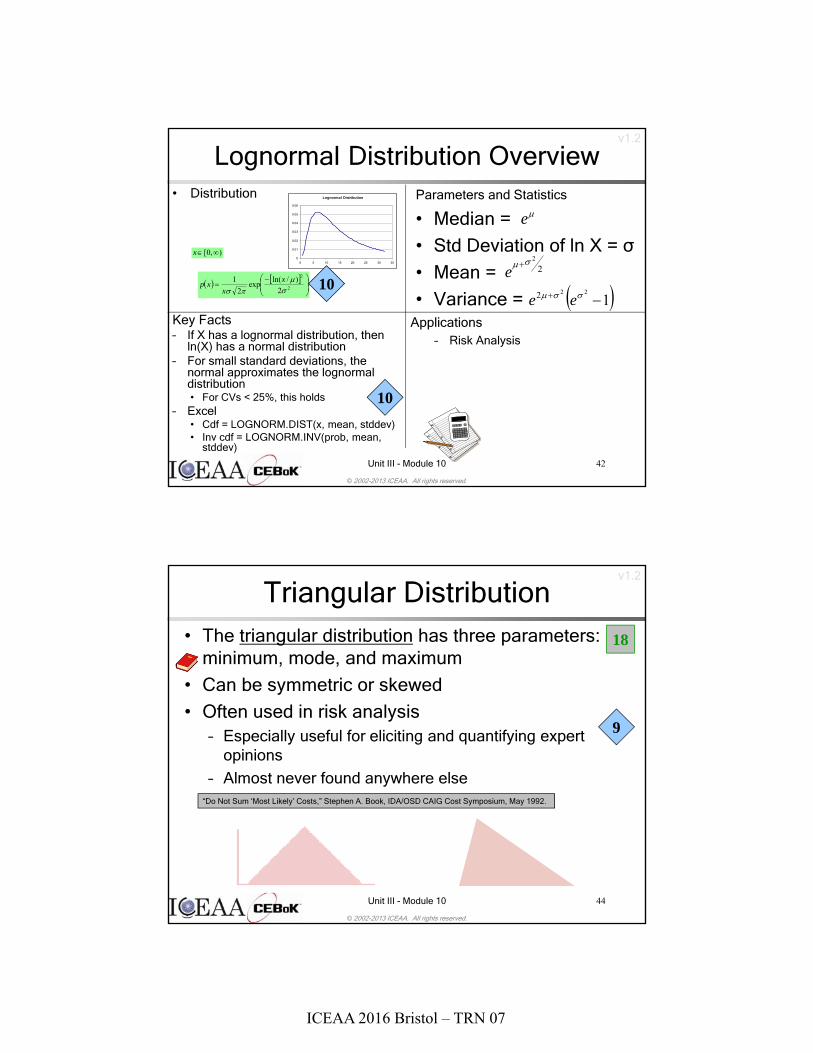
Lognormal Distribution Overview• Distribution Parameters and Statistics
• Median =
• Std Deviation of ln X = σ
• Mean =
• Variance = Key Facts– If X has a lognormal distribution, then
ln(X) has a normal distribution– For small standard deviations, the
normal approximates the lognormal distribution• For CVs < 25%, this holds
– Excel• Cdf = LOGNORM.DIST(x, mean, stddev)• Inv cdf = LOGNORM.INV(prob, mean,
stddev)
Applications– Risk Analysis
2
2
2
)/ln(exp
2
1
x
xxp
22
e
1222 ee
Lognormal Distribution
0
0.01
0.02
0.03
0.04
0.05
0.06
0 5 10 15 20 25 30 35
),0[ x
10
e
10
v1.2
© 2002-2013 ICEAA. All rights reserved.
Unit III - Module 10 44
Triangular Distribution• The triangular distribution has three parameters:
minimum, mode, and maximum
• Can be symmetric or skewed
• Often used in risk analysis– Especially useful for eliciting and quantifying expert
opinions
– Almost never found anywhere else
9
18
“Do Not Sum ‘Most Likely’ Costs,” Stephen A. Book, IDA/OSD CAIG Cost Symposium, May 1992.
ICEAA 2016 Bristol – TRN 07
v1.2
© 2002-2013 ICEAA. All rights reserved.
Unit III - Module 10 45
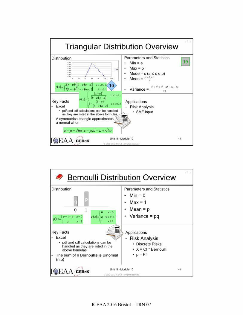
Triangular Distribution OverviewDistribution Parameters and Statistics
• Min = a• Max = b• Mode = c (a ≤ c ≤ b)• Mean =
• Variance =
Key Facts– Excel
• pdf and cdf calculations can be handled as they are listed in the above formulas
– A symmetrical triangle approximatesa normal when
Applications– Risk Analysis
• SME Input
bxccbabxb
cxaacabaxxp
/2
/2
bxc
cbab
xb
cxaacab
ax
xF 2
2
1
6,,6 bca
3
cba
18
222 bcacabcba
0.0000.0050.0100.015
0.0200.0250.0300.035
0 20 40 60 80 100 120
19
10
v1.2
© 2002-2013 ICEAA. All rights reserved.
Unit III - Module 10 46
Bernoulli Distribution OverviewDistribution Parameters and Statistics
• Min = 0
• Max = 1
• Mean = p
• Variance = pq
Key Facts– Excel
• pdf and cdf calculations can be handled as they are listed in the above formulas
– The sum of n Bernoullis is Binomial (n,p)
Applications
– Risk Analysis• Discrete Risks• X = Cf * Bernoulli• p = Pf
1
01
xp
xpqxp
11
10
00
x
xq
x
xF
q p
0 1
ICEAA 2016 Bristol – TRN 07
v1.2
© 2002-2013 ICEAA. All rights reserved.
Unit III - Module 10 101
1
rnb
ra
X r
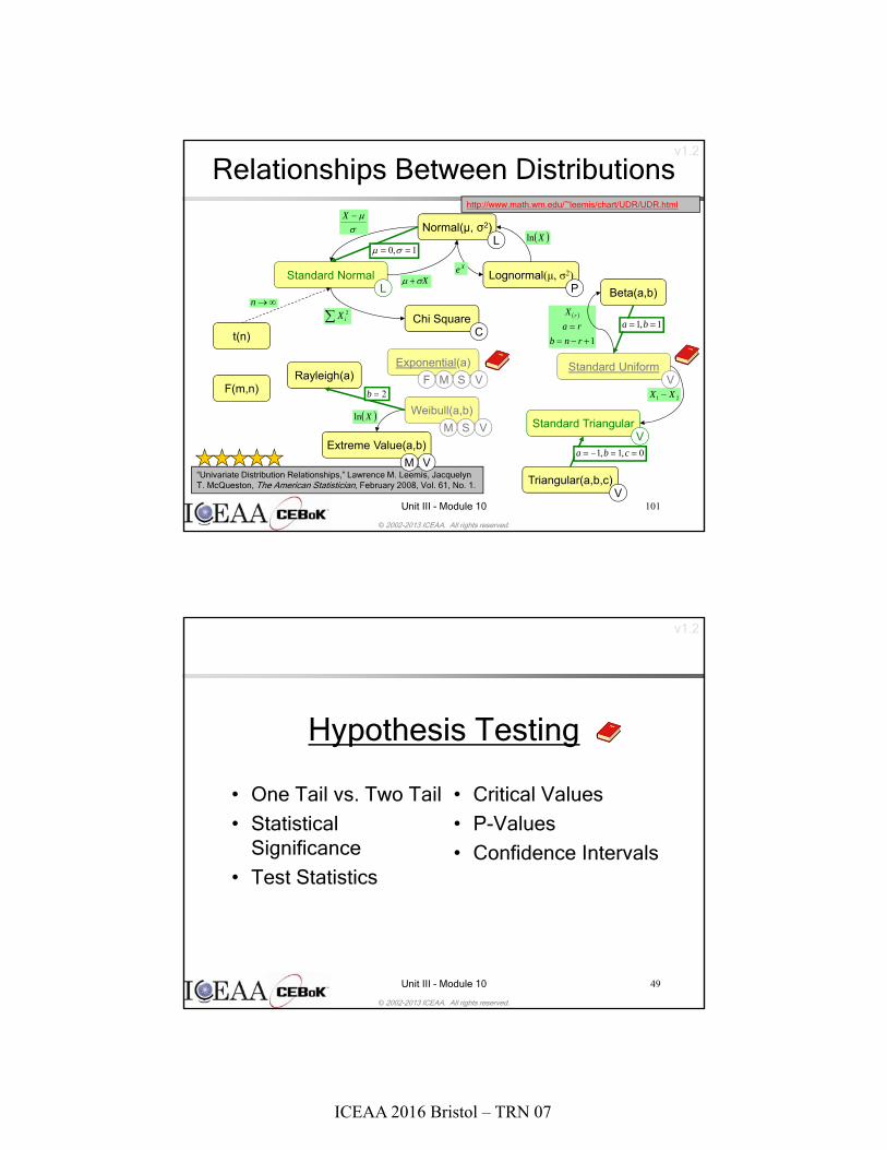
Relationships Between Distributions
“Univariate Distribution Relationships,” Lawrence M. Leemis, Jacquelyn T. McQueston, The American Statistician, February 2008, Vol. 61, No. 1. Triangular(a,b,c)
Standard Triangular
Standard Uniform
Standard Normal
Normal(μ, σ2)
Lognormal(μ, σ2)
Chi Square
t(n)
L
F(m,n)
Beta(a,b)
Exponential(a)
Weibull(a,b)
Rayleigh(a)
Extreme Value(a,b)
X
X
L1,0
2iX
nP
Xln
Xe
1,1 ba
21 XX
0,1,1 cba
C
V
V
V
VSMF
VSM
VM
Xln
2b
http://www.math.wm.edu/~leemis/chart/UDR/UDR.html
v1.2
© 2002-2013 ICEAA. All rights reserved.
Unit III - Module 10 49
Hypothesis Testing
• One Tail vs. Two Tail
• Statistical Significance
• Test Statistics
• Critical Values
• P-Values
• Confidence Intervals
ICEAA 2016 Bristol – TRN 07
v1.2
© 2002-2013 ICEAA. All rights reserved.
Unit III - Module 10 50
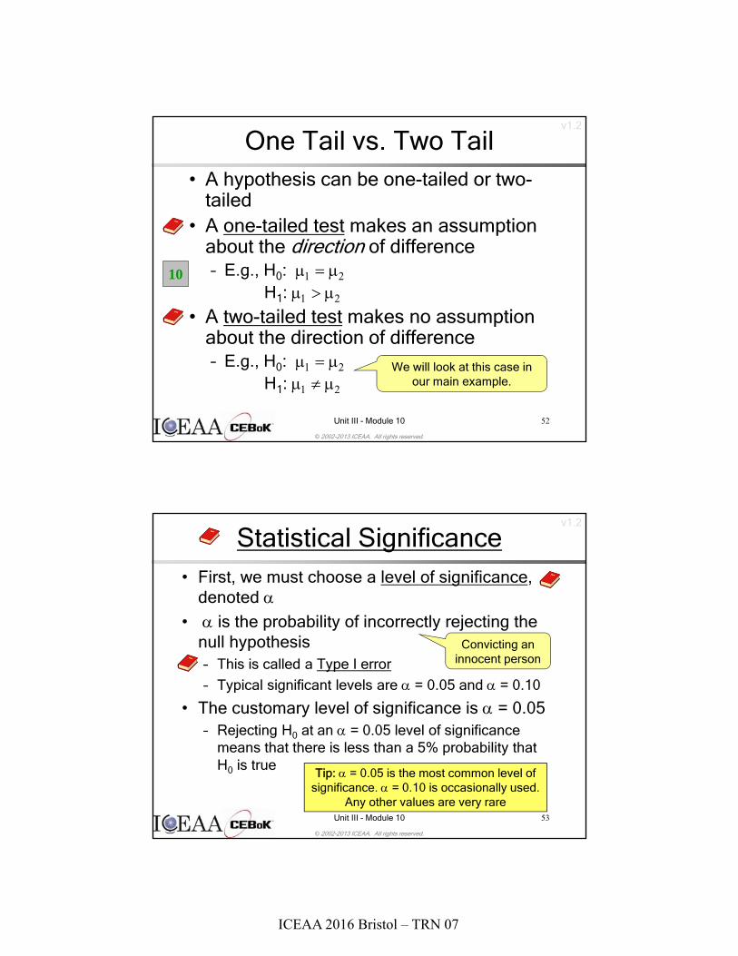
Hypothesis Test
• Hypothesis tests are often used to test for differences between population groups
• Two hypotheses are proposed:– H0 is the null hypothesis
• H0 is presumed to be true unless the data is proven to contradict the null hypothesis
– H1 is the alternative hypothesis• H1 may only be accepted with statistical
evidence contradicting the null hypothesis
“innocent until proven guilty”
“beyond a reasonable
doubt”
v1.2
© 2002-2013 ICEAA. All rights reserved.
Unit III - Module 10 51
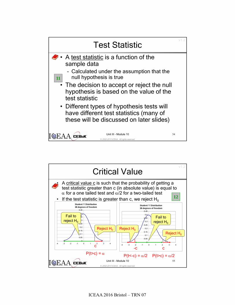
Examples of Hypotheses• Test to see if two populations have different
meansH0: (the means are the same)H1: (the means are different)
• Test to see if two populations have different standard deviationsH0: (the std devs are the same)H1: (the std devs are different)
• Test to see if two populations are identically distributedH0: f(x) = g(x) (the distributions are the same)H1: f(x) g(x) (the distributions are different)
F test
Chi Square or K-S test
t test
ICEAA 2016 Bristol – TRN 07
v1.2
© 2002-2013 ICEAA. All rights reserved.
Unit III - Module 10 52
One Tail vs. Two Tail• A hypothesis can be one-tailed or two-
tailed• A one-tailed test makes an assumption
about the direction of difference– E.g., H0:
H1: • A two-tailed test makes no assumption
about the direction of difference– E.g., H0:
H1: We will look at this case in
our main example.
10
v1.2
© 2002-2013 ICEAA. All rights reserved.
Unit III - Module 10 53
Statistical Significance• First, we must choose a level of significance,
denoted • is the probability of incorrectly rejecting the
null hypothesis – This is called a Type I error
– Typical significant levels are = 0.05 and = 0.10
• The customary level of significance is = 0.05– Rejecting H0 at an = 0.05 level of significance
means that there is less than a 5% probability that H0 is true
Convicting an innocent person
Tip: = 0.05 is the most common level of significance. = 0.10 is occasionally used.
Any other values are very rare
ICEAA 2016 Bristol – TRN 07
v1.2
© 2002-2013 ICEAA. All rights reserved.
Unit III - Module 10 54
Test Statistic• A test statistic is a function of the
sample data– Calculated under the assumption that the
null hypothesis is true
• The decision to accept or reject the null hypothesis is based on the value of the test statistic
• Different types of hypothesis tests will have different test statistics (many of these will be discussed on later slides)
11
v1.2
© 2002-2013 ICEAA. All rights reserved.
Unit III - Module 10 55
Critical Value
Student 't' Distribution38 degrees of freedom
0
0.05
0.1
0.15
0.2
0.25
0.3
0.35
0.4
0.45
-4 -3 -2 -1 0 1 2 3 4
Student 't' Distribution38 degrees of freedom
0
0.05
0.1
0.15
0.2
0.25
0.3
0.35
0.4
0.45
-4 -3 -2 -1 0 1 2 3 4
Fail to reject H0
Reject H0
Reject H0
c
P(t>c) = /2
-c
P(t<-c) = /2
Fail to reject H0
Reject H0
c
P(t>c) =
• A critical value c is such that the probability of getting a test statistic greater than c (in absolute value) is equal to for a one tailed test and /2 for a two-tailed test
• If the test statistic is greater than c, we reject H012

ICEAA 2016 Bristol – TRN 07
v1.2
© 2002-2013 ICEAA. All rights reserved.
Unit III - Module 10 56
Example Problem• Suppose we have historical cost growth
factors from a set of DoD programs and a set of NAVAIR programs
• We wish to see if cost growth for NAVAIR programs differs from DoD-wide growth
• The hypotheses are:H0: N = D (the means are the same)H1: N D (the means are different)
• This is a two-tailed test as we are making no assumptions as to whether or not NAVAIR has higher or lower growth than DoD
“NAVAIR Cost Growth Study,” R.L. Coleman, M.E. Dameron, C.L. Pullen, J.R. Summerville, D.M. Snead, 34th DoDCAS and ISPA/SCEA 2001.
v1.2
© 2002-2013 ICEAA. All rights reserved.
Unit III - Module 10 57
Example Problem Data
• Suppose we have the following cost growth factors
(CGF) for DoD and NAVAIR programs
• Average DoD CGF = 1.19
• Average NAVAIR CGF = 1.33
DoD NAVAIR1.26 1.261.44 1.920.96 1.640.93 1.831.26 1.850.88 1.031.10 1.081.23 1.440.76 1.601.75 1.241.80 1.041.56 1.211.24 1.111.51 1.310.93 1.470.49 1.251.29 1.110.76 1.151.21 1.111.50 0.90
But is this a “real” difference, or did it
happen by chance?

ICEAA 2016 Bristol – TRN 07
v1.2
© 2002-2013 ICEAA. All rights reserved.
Unit III - Module 10 58
Example Test Statistic• For each different type of hypothesis test, there is a
corresponding test statistic• In our example problem, we will be using the two-
sample t-test for means– Let Xn ~ N(x, 2) and Ym ~ N(y, 2) where X and Y are
independent– Let Sx
2 and Sy2 be the two sample variances
– Let Sp2 be the pooled variance, where
– Then,
has a t distribution with (n + m – 2) degrees of freedom
2
)1()1( 222
mn
SmSnS YX
p
mnS
YXT
p
YX
11
)(
v1.2
© 2002-2013 ICEAA. All rights reserved.
Unit III - Module 10 59
Example Test StatisticCalculation
• Using our example problem data, we get the following:
• X = 1.19, Y = 1.33• Sx
2 = 0.12, Sy2 = 0.09
• Sp2 = (20-1)(0.12) + (20-1)(0.09)
20 + 20 – 2
= 0.11• If H0 is true, then (x – y) = 0• So, under H0,
DoD NAVAIR1.26 1.261.44 1.920.96 1.640.93 1.831.26 1.850.88 1.031.10 1.081.23 1.440.76 1.601.75 1.241.80 1.041.56 1.211.24 1.111.51 1.310.93 1.470.49 1.251.29 1.110.76 1.151.21 1.111.50 0.90
32.1
)201
201
0.11(
0 - 1.33 - 1.19 T
59

ICEAA 2016 Bristol – TRN 07
v1.2
© 2002-2013 ICEAA. All rights reserved.
Unit III - Module 10 60
Example Critical Values
Student 't' Distribution38 degrees of freedom
0
0.05
0.1
0.15
0.2
0.25
0.3
0.35
0.4
0.45
-4 -3 -2 -1 0 1 2 3 4
The critical value for = 0.05 and 38 df is 2.02
P(t > 2.02) = /2 = 0.025
P(t < -2.02) = /2 = 0.025
The test statistic for our example is
T = –1.32
Since we do not have T < -2.02 or T > 2.02, we fail to reject the null hypothesis. There is no statistical difference between the two means at = 0.05
v1.2
© 2002-2013 ICEAA. All rights reserved.
Unit III - Module 10 61
Example t TestUsing Excel
DoD NAVAIRMean 1.193094 1.327704Variance 0.117941 0.089239Observations 20 20Pooled Variance 0.10359Hypothesized Mean Difference 0df 38t Stat -1.322571P(T<=t) one-tail 0.096942t Critical one-tail 1.685953P(T<=t) two-tail 0.193883t Critical two-tail 2.024394
DoD NAVAIRMean 1.193094 1.327704Variance 0.117941 0.089239Observations 20 20Pooled Variance 0.10359Hypothesized Mean Difference 0df 38t Stat -1.322571P(T<=t) one-tail 0.096942t Critical one-tail 1.685953P(T<=t) two-tail 0.193883t Critical two-tail 2.024394
test statistic for our example
Critical value for a one-tailed test. In this case, we would
still fail to reject H0
Critical value for our two-tailed test. Fail to reject
the null hypothesis.
• In Excel, use the Data Analysis Add-In to run a t test
Tip: The Excel default significance level is
= 0.05
Warning: Results of macros do not update if your data
change!
ICEAA 2016 Bristol – TRN 07
v1.2
© 2002-2013 ICEAA. All rights reserved.
Student 't' Distribution38 degrees of freedom
0
0.05
0.1
0.15
0.2
0.25
0.3
0.35
0.4
0.45
-4 -3 -2 -1 0 1 2 3 4
Unit III - Module 10 62
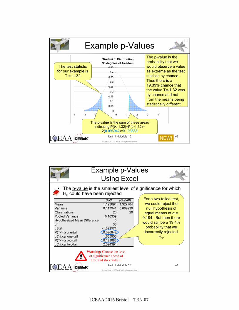
Example p-Values
The test statistic for our example is
T = –1.32
The p-value is the probability that we would observe a value as extreme as the test statistic by chance. Thus there is a 19.39% chance that the value T=-1.32 was by chance and not from the means being statistically different.
The p-value is the sum of these areas indicating P(t<-1.32)+P(t>1.32)=
2(0.096942)=0.193883
NEW!
v1.2
© 2002-2013 ICEAA. All rights reserved.
Unit III - Module 10 63
Example p-Values Using Excel
DoD NAVAIRMean 1.193094 1.327704Variance 0.117941 0.089239Observations 20 20Pooled Variance 0.10359Hypothesized Mean Difference 0df 38t Stat -1.322571P(T<=t) one-tail 0.096942t Critical one-tail 1.685953P(T<=t) two-tail 0.193883t Critical two-tail 2.024394
DoD NAVAIRMean 1.193094 1.327704Variance 0.117941 0.089239Observations 20 20Pooled Variance 0.10359Hypothesized Mean Difference 0df 38t Stat -1.322571P(T<=t) one-tail 0.096942t Critical one-tail 1.685953P(T<=t) two-tail 0.193883t Critical two-tail 2.024394
For a two-tailed test, we could reject the null hypothesis of
equal means at α = 0.194. But then there would still be a 19.4%
probability that we incorrectly rejected
H0.
• The p-value is the smallest level of significance for which H0 could have been rejected
Warning: Choose the level of significance ahead of time and stick with it!
ICEAA 2016 Bristol – TRN 07
v1.2
© 2002-2013 ICEAA. All rights reserved.
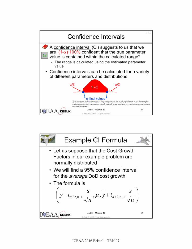
Unit III - Module 10 64
• A confidence interval (CI) suggests to us that we are (1-)·100% confident that the true parameter value is contained within the calculated range*– The range is calculated using the estimated parameter
value
• Confidence intervals can be calculated for a variety of different parameters and distributions
Confidence Intervals
1 - /2 /2
critical values
13
* Note this statement provides a general sense of what a confidence interval does for us in concise language for ease of understanding. The specific statistical interpretation is that if many independent samples are taken where the levels of the predictor variable are the same as in the data set, and a (1-)*100% confidence interval is constructed for each sample, then (1-) ·100% of the intervals will contain the true value of the parameter.
v1.2
© 2002-2013 ICEAA. All rights reserved.
Unit III - Module 10 65
Example CI Formula
• Let us suppose that the Cost Growth Factors in our example problem are normally distributed
• We will find a 95% confidence interval for the average DoD cost growth
• The formula is
n
sty
n
sty nn 1,2/1,2/ ,,
ICEAA 2016 Bristol – TRN 07
v1.2
© 2002-2013 ICEAA. All rights reserved.
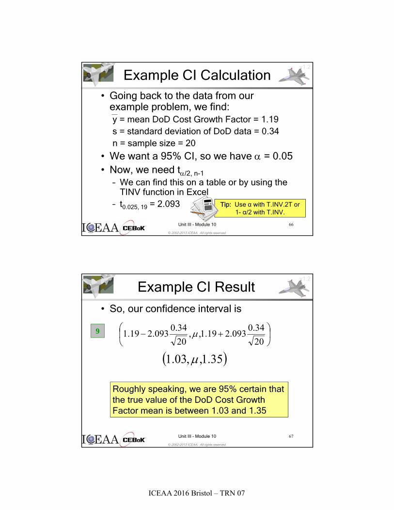
Unit III - Module 10 66
Example CI Calculation• Going back to the data from our
example problem, we find:y = mean DoD Cost Growth Factor = 1.19s = standard deviation of DoD data = 0.34 n = sample size = 20
• We want a 95% CI, so we have = 0.05• Now, we need t/2, n-1
– We can find this on a table or by using the TINV function in Excel
– t0.025, 19 = 2.093 Tip: Use α with T.INV.2T or1- α/2 with T.INV.
v1.2
© 2002-2013 ICEAA. All rights reserved.
Unit III - Module 10 67
Example CI Result
• So, our confidence interval is
20
34.0093.219.1,,
20
34.0093.219.1
35.1,,03.1
Roughly speaking, we are 95% certain that the true value of the DoD Cost Growth Factor mean is between 1.03 and 1.35
9

ICEAA 2016 Bristol – TRN 07
v1.2
© 2002-2013 ICEAA. All rights reserved.
Unit III - Module 10 75
Prob/Stat Summary• A solid understanding of probability and
statistics is vital to both cost and risk analysis• Descriptive statistics are used to characterize,
describe, and compare the data– Central Tendency – mean, median, mode– Dispersion – variance, standard deviation,
coefficient of variation
• Inferential statistics are used to draw inferences from the data– Testing multiple population groups for differences
in means, variances, distributions, etc.– Confidence intervals around estimates