CHAPTER 7 FLEXIBLE BUDGETS, DIRECT-COST … 7 FLEXIBLE BUDGETS, DIRECT-COST VARIANCES, AND MANAGEMENT CONTROL ... cost management, (ii) pricing decisions,

7-1

CHAPTER 7 FLEXIBLE BUDGETS, DIRECT-COST VARIANCES,

AND MANAGEMENT CONTROL 7-1 Management by exception is the practice of concentrating on areas not operating as expected and giving less attention to areas operating as expected. Variance analysis helps managers identify areas not operating as expected. The larger the variance, the more likely an area is not operating as expected. 7-2 Two sources of information about budgeted amounts are (a) past amounts and (b) detailed engineering studies. 7-3 A favorable variance––denoted F––is a variance that has the effect of increasing operating income relative to the budgeted amount. An unfavorable variance––denoted U––is a variance that has the effect of decreasing operating income relative to the budgeted amount. 7-4 The key difference is the output level used to set the budget. A static budget is based on the level of output planned at the start of the budget period. A flexible budget is developed using budgeted revenues or cost amounts based on the actual output level in the budget period. The actual level of output is not known until the end of the budget period. 7-5 A flexible-budget analysis enables a manager to distinguish how much of the difference between an actual result and a budgeted amount is due to (a) the difference between actual and budgeted output levels, and (b) the difference between actual and budgeted selling prices, variable costs, and fixed costs. 7-6 The steps in developing a flexible budget are:

Step 1: Identify the actual quantity of output. Step 2: Calculate the flexible budget for revenues based on budgeted selling price and

actual quantity of output. Step 3: Calculate the flexible budget for costs based on budgeted variable cost per output

unit, actual quantity of output, and budgeted fixed costs. 7-7 Four reasons for using standard costs are:

(i) cost management, (ii) pricing decisions, (iii) budgetary planning and control, and (iv) financial statement preparation.

7-8 A manager should subdivide the flexible-budget variance for direct materials into a price variance (that reflects the difference between actual and budgeted prices of direct materials) and an efficiency variance (that reflects the difference between the actual and budgeted quantities of direct materials used to produce actual output). The individual causes of these variances can then be investigated, recognizing possible interdependencies across these individual causes.

7-2

7-9 Possible causes of a favorable direct materials price variance are: • purchasing officer negotiated more skillfully than was planned in the budget, • purchasing manager bought in larger lot sizes than budgeted, thus obtaining quantity

discounts, • materials prices decreased unexpectedly due to, say, industry oversupply, • budgeted purchase prices were set without careful analysis of the market, and • purchasing manager received unfavorable terms on nonpurchase price factors (such as

lower quality materials). 7-10 Some possible reasons for an unfavorable direct manufacturing labor efficiency variance are the hiring and use of underskilled workers; inefficient scheduling of work so that the workforce was not optimally occupied; poor maintenance of machines resulting in a high proportion of non-value-added labor; unrealistic time standards. Each of these factors would result in actual direct manufacturing labor-hours being higher than indicated by the standard work rate. 7-11 Variance analysis, by providing information about actual performance relative to standards, can form the basis of continuous operational improvement. The underlying causes of unfavorable variances are identified and corrective action taken where possible. Favorable variances can also provide information if the organization can identify why a favorable variance occurred. Steps can often be taken to replicate those conditions more often. As the easier changes are made, and perhaps some standards tightened, the harder issues will be revealed for the organization to act on—this is continuous improvement. 7-12 An individual business function, such as production, is interdependent with other business functions. Factors outside of production can explain why variances arise in the production area. For example:

• poor design of products or processes can lead to a sizable number of defects, • marketing personnel making promises for delivery times that require a large number

of rush orders can create production-scheduling difficulties, and • purchase of poor-quality materials by the purchasing manager can result in defects

and waste. 7-13 The plant supervisor likely has good grounds for complaint if the plant accountant puts excessive emphasis on using variances to pin blame. The key value of variances is to help understand why actual results differ from budgeted amounts and then to use that knowledge to promote learning and continuous improvement. 7-14 The sales-volume variance can be decomposed into two parts: a market-share variance that reflects the difference in budgeted contribution margin due to the actual market share being different from the budgeted share; and a market-size variance, which captures the impact of actual size of the market as a while differing from the budgeted market size. 7-15 Evidence on the costs of other companies is one input managers can use in setting the performance measure for next year. However, caution should be taken before choosing such an amount as next year's performance measure. It is important to understand why cost differences across companies exist and whether these differences can be eliminated. It is also important to examine when planned changes (in, say, technology) next year make even the current low-cost producer not a demanding enough hurdle.

7-3

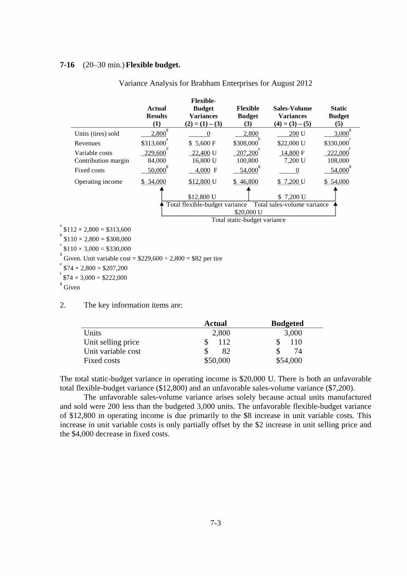
7-16 (20–30 min.) Flexible budget.

Variance Analysis for Brabham Enterprises for August 2012

Actual Results

(1)

Flexible-Budget

Variances (2) = (1) – (3)

Flexible Budget

(3)

Sales-Volume Variances

(4) = (3) – (5)

Static Budget

(5) Units (tires) sold 2,800

g 0 2,800 200 U 3,000

g

Revenues $313,600a $ 5,600 F $308,000

b $22,000 U $330,000

c

Variable costs 229,600d 22,400 U 207,200

e 14,800 F 222,000

f

Contribution margin 84,000 16,800 U 100,800 7,200 U 108,000 Fixed costs 50,000

g 4,000 F 54,000

g 0 54,000

g

Operating income $ 34,000 $12,800 U $ 46,800 $ 7,200 U $ 54,000 $12,800 U $ 7,200 U Total flexible-budget variance Total sales-volume variance $20,000 U Total static-budget variance a $112 × 2,800 = $313,600 b $110 × 2,800 = $308,000 c $110 × 3,000 = $330,000 d Given. Unit variable cost = $229,600 ÷ 2,800 = $82 per tire e $74 × 2,800 = $207,200 f $74 × 3,000 = $222,000 g Given 2. The key information items are:

Actual Budgeted Units Unit selling price Unit variable cost Fixed costs

2,800 $ 112 $ 82 $50,000

3,000 $ 110 $ 74 $54,000

The total static-budget variance in operating income is $20,000 U. There is both an unfavorable total flexible-budget variance ($12,800) and an unfavorable sales-volume variance ($7,200). The unfavorable sales-volume variance arises solely because actual units manufactured and sold were 200 less than the budgeted 3,000 units. The unfavorable flexible-budget variance of $12,800 in operating income is due primarily to the $8 increase in unit variable costs. This increase in unit variable costs is only partially offset by the $2 increase in unit selling price and the $4,000 decrease in fixed costs.

7-4

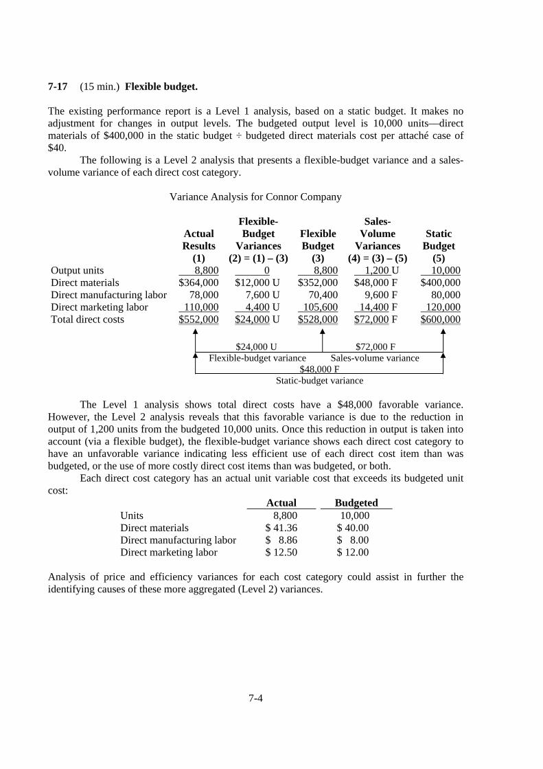
7-17 (15 min.) Flexible budget. The existing performance report is a Level 1 analysis, based on a static budget. It makes no adjustment for changes in output levels. The budgeted output level is 10,000 units––direct materials of $400,000 in the static budget ÷ budgeted direct materials cost per attaché case of $40. The following is a Level 2 analysis that presents a flexible-budget variance and a sales-volume variance of each direct cost category.

Variance Analysis for Connor Company

Actual Results

(1)

Flexible- Budget

Variances (2) = (1) – (3)

FlexibleBudget

(3)

Sales- Volume

Variances (4) = (3) – (5)

Static

Budget (5)

Output units Direct materials Direct manufacturing labor Direct marketing labor Total direct costs

8,800 $364,000 78,000 110,000 $552,000

0 $12,000 U

7,600 U 4,400 U $24,000 U

8,800$352,000 70,400 105,600$528,000

1,200 U $48,000 F

9,600 F 14,400 F $72,000 F

10,000$400,000 80,000 120,000$600,000

$24,000 U $72,000 F Flexible-budget variance Sales-volume variance $48,000 F Static-budget variance The Level 1 analysis shows total direct costs have a $48,000 favorable variance. However, the Level 2 analysis reveals that this favorable variance is due to the reduction in output of 1,200 units from the budgeted 10,000 units. Once this reduction in output is taken into account (via a flexible budget), the flexible-budget variance shows each direct cost category to have an unfavorable variance indicating less efficient use of each direct cost item than was budgeted, or the use of more costly direct cost items than was budgeted, or both.

Each direct cost category has an actual unit variable cost that exceeds its budgeted unit cost:

Actual Budgeted Units Direct materials Direct manufacturing labor Direct marketing labor

8,800 $ 41.36 $ 8.86 $ 12.50

10,000 $ 40.00 $ 8.00 $ 12.00

Analysis of price and efficiency variances for each cost category could assist in further the identifying causes of these more aggregated (Level 2) variances.

7-5

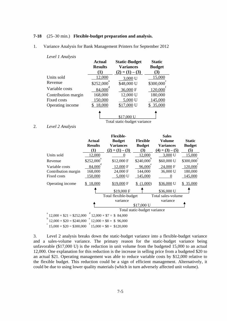
7-18 (25–30 min.) Flexible-budget preparation and analysis. 1. Variance Analysis for Bank Management Printers for September 2012

Level 1 Analysis Actual

Results (1)

Static-BudgetVariances

(2) = (1) – (3)

Static Budget

(3) Units sold Revenue

12,000 $252,000

a

3,000 U $48,000 U

15,000 $300,000

c

Variable costs 84,000d 36,000 F 120,000

f

Contribution margin Fixed costs Operating income

168,000 150,000 $ 18,000

12,000 U 5,000 U $17,000 U

180,000 145,000 $ 35,000

$17,000 U Total static-budget variance 2. Level 2 Analysis

Actual Results

(1)

Flexible- Budget

Variances (2) = (1) – (3)

Flexible Budget

(3)

Sales

Volume Variances

(4) = (3) – (5)

Static Budget

(5) Units sold 12,000 0 12,000 3,000 U 15,000 Revenue $252,000

a $12,000 F $240,000

b $60,000 U $300,000

c

Variable costs 84,000d 12,000 F 96,000

e 24,000 F 120,000

f

Contribution margin 168,000 24,000 F 144,000 36,000 U 180,000 Fixed costs 150,000 5,000 U 145,000 0 145,000

Operating income $ 18,000 $19,000 F $ (1,000) $36,000 U $ 35,000

$19,000 F $36,000 U Total flexible-budget Total sales-volume variance variance $17,000 U Total static-budget variance

a 12,000 × $21 = $252,000 d 12,000 × $7 = $ 84,000

b 12,000 × $20 = $240,000 e 12,000 × $8 = $ 96,000

c 15,000 × $20 = $300,000 f 15,000 × $8 = $120,000

3. Level 2 analysis breaks down the static-budget variance into a flexible-budget variance and a sales-volume variance. The primary reason for the static-budget variance being unfavorable ($17,000 U) is the reduction in unit volume from the budgeted 15,000 to an actual 12,000. One explanation for this reduction is the increase in selling price from a budgeted $20 to an actual $21. Operating management was able to reduce variable costs by $12,000 relative to the flexible budget. This reduction could be a sign of efficient management. Alternatively, it could be due to using lower quality materials (which in turn adversely affected unit volume).

7-6

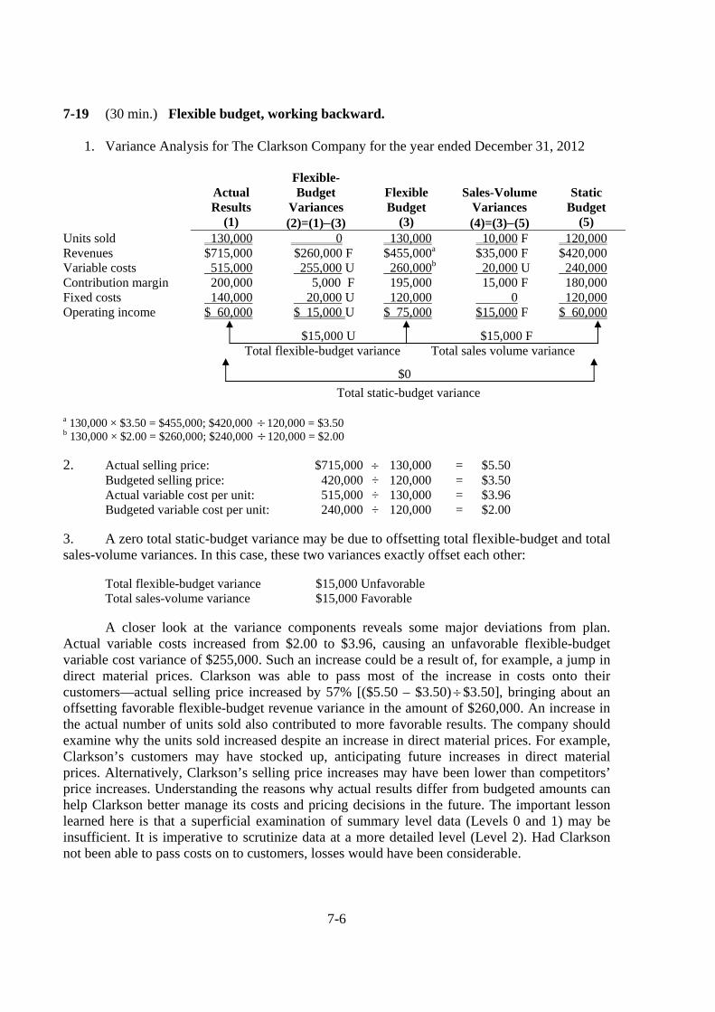
7-19 (30 min.) Flexible budget, working backward.

1. Variance Analysis for The Clarkson Company for the year ended December 31, 2012

Actual Results

(1)

Flexible- Budget

Variances (2)=(1)−(3)

Flexible Budget

(3)

Sales-Volume

Variances (4)=(3)−(5)

Static

Budget (5)

Units sold 130,000 0 130,000 10,000 F 120,000 Revenues $715,000 $260,000 F $455,000a $35,000 F $420,000 Variable costs 515,000 255,000 U 260,000b 20,000 U 240,000 Contribution margin 200,000 5,000 F 195,000 15,000 F 180,000 Fixed costs 140,000 20,000 U 120,000 0 120,000 Operating income $ 60,000 $ 15,000 U $ 75,000 $15,000 F $ 60,000

a 130,000 × $3.50 = $455,000; $420,000 ÷ 120,000 = $3.50 b 130,000 × $2.00 = $260,000; $240,000 ÷120,000 = $2.00 2. Actual selling price: $715,000 ÷ 130,000 = $5.50 Budgeted selling price: 420,000 ÷ 120,000 = $3.50 Actual variable cost per unit: 515,000 ÷ 130,000 = $3.96 Budgeted variable cost per unit: 240,000 ÷ 120,000 = $2.00 3. A zero total static-budget variance may be due to offsetting total flexible-budget and total sales-volume variances. In this case, these two variances exactly offset each other: Total flexible-budget variance $15,000 Unfavorable Total sales-volume variance $15,000 Favorable A closer look at the variance components reveals some major deviations from plan. Actual variable costs increased from $2.00 to $3.96, causing an unfavorable flexible-budget variable cost variance of $255,000. Such an increase could be a result of, for example, a jump in direct material prices. Clarkson was able to pass most of the increase in costs onto their customers—actual selling price increased by 57% [($5.50 – $3.50)÷$3.50], bringing about an offsetting favorable flexible-budget revenue variance in the amount of $260,000. An increase in the actual number of units sold also contributed to more favorable results. The company should examine why the units sold increased despite an increase in direct material prices. For example, Clarkson’s customers may have stocked up, anticipating future increases in direct material prices. Alternatively, Clarkson’s selling price increases may have been lower than competitors’ price increases. Understanding the reasons why actual results differ from budgeted amounts can help Clarkson better manage its costs and pricing decisions in the future. The important lesson learned here is that a superficial examination of summary level data (Levels 0 and 1) may be insufficient. It is imperative to scrutinize data at a more detailed level (Level 2). Had Clarkson not been able to pass costs on to customers, losses would have been considerable.

$15,000 U Total flexible-budget variance

$15,000 F Total sales volume variance

$0 Total static-budget variance

7-7

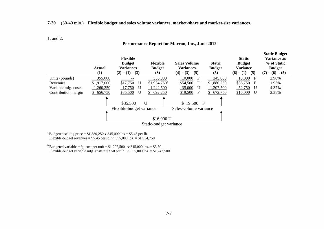
7-20 (30-40 min.) Flexible budget and sales volume variances, market-share and market-size variances. 1. and 2.

Performance Report for Marron, Inc., June 2012

Actual

Flexible Budget

Variances Flexible Budget

Sales Volume Variances

Static Budget

Static Budget

Variance

Static Budget Variance as % of Static

Budget (1) (2) = (1) – (3) (3) (4) = (3) – (5) (5) (6) = (1) – (5) (7) = (6) ÷ (5) Units (pounds) 355,000 -- 355,000 10,000 F 345,000 10,000 F 2.90% Revenues $1,917,000 $17,750 U $1,934,750a $54,500 F $1,880,250 $36,750 F 1.95% Variable mfg. costs 1,260,250 17,750 U 1,242,500b 35,000 U 1,207,500 52,750 U 4.37% Contribution margin $ 656,750 $35,500 U $ 692,250 $19,500 F $ 672,750 $16,000 U 2.38% $35,500 U $ 19,500 F Flexible-budget variance Sales-volume variance

$16,000 U Static-budget variance a Budgeted selling price = $1,880,250÷ 345,000 lbs = $5.45 per lb. Flexible-budget revenues = $5.45 per lb. × 355,000 lbs. = $1,934,750 b Budgeted variable mfg. cost per unit = $1,207,500 ÷ 345,000 lbs. = $3.50 Flexible-budget variable mfg. costs = $3.50 per lb. × 355,000 lbs. = $1,242,500

7-8

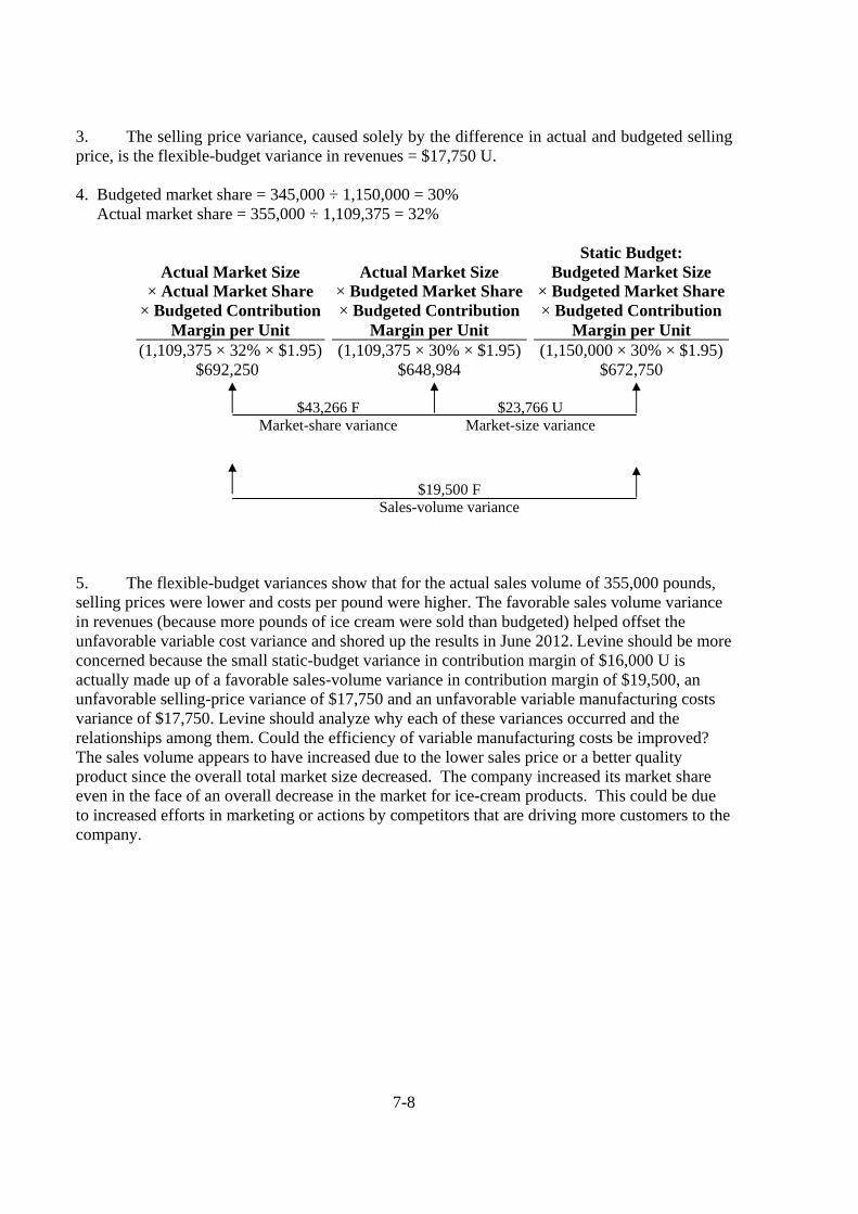
3. The selling price variance, caused solely by the difference in actual and budgeted selling price, is the flexible-budget variance in revenues = $17,750 U. 4. Budgeted market share = 345,000 ÷ 1,150,000 = 30% Actual market share = 355,000 ÷ 1,109,375 = 32%

Actual Market Size

× Actual Market Share × Budgeted Contribution

Margin per Unit

Actual Market Size

× Budgeted Market Share× Budgeted Contribution

Margin per Unit

Static Budget: Budgeted Market Size


Margin per Unit (1,109,375 × 32% × $1.95)

$692,250 (1,109,375 × 30% × $1.95)

$648,984 (1,150,000 × 30% × $1.95)

$672,750 $43,266 F $23,766 U Market-share variance Market-size variance

5. The flexible-budget variances show that for the actual sales volume of 355,000 pounds, selling prices were lower and costs per pound were higher. The favorable sales volume variance in revenues (because more pounds of ice cream were sold than budgeted) helped offset the unfavorable variable cost variance and shored up the results in June 2012. Levine should be more concerned because the small static-budget variance in contribution margin of $16,000 U is actually made up of a favorable sales-volume variance in contribution margin of $19,500, an unfavorable selling-price variance of $17,750 and an unfavorable variable manufacturing costs variance of $17,750. Levine should analyze why each of these variances occurred and the relationships among them. Could the efficiency of variable manufacturing costs be improved? The sales volume appears to have increased due to the lower sales price or a better quality product since the overall total market size decreased. The company increased its market share even in the face of an overall decrease in the market for ice-cream products. This could be due to increased efforts in marketing or actions by competitors that are driving more customers to the company.

$19,500 F Sales-volume variance

7-9

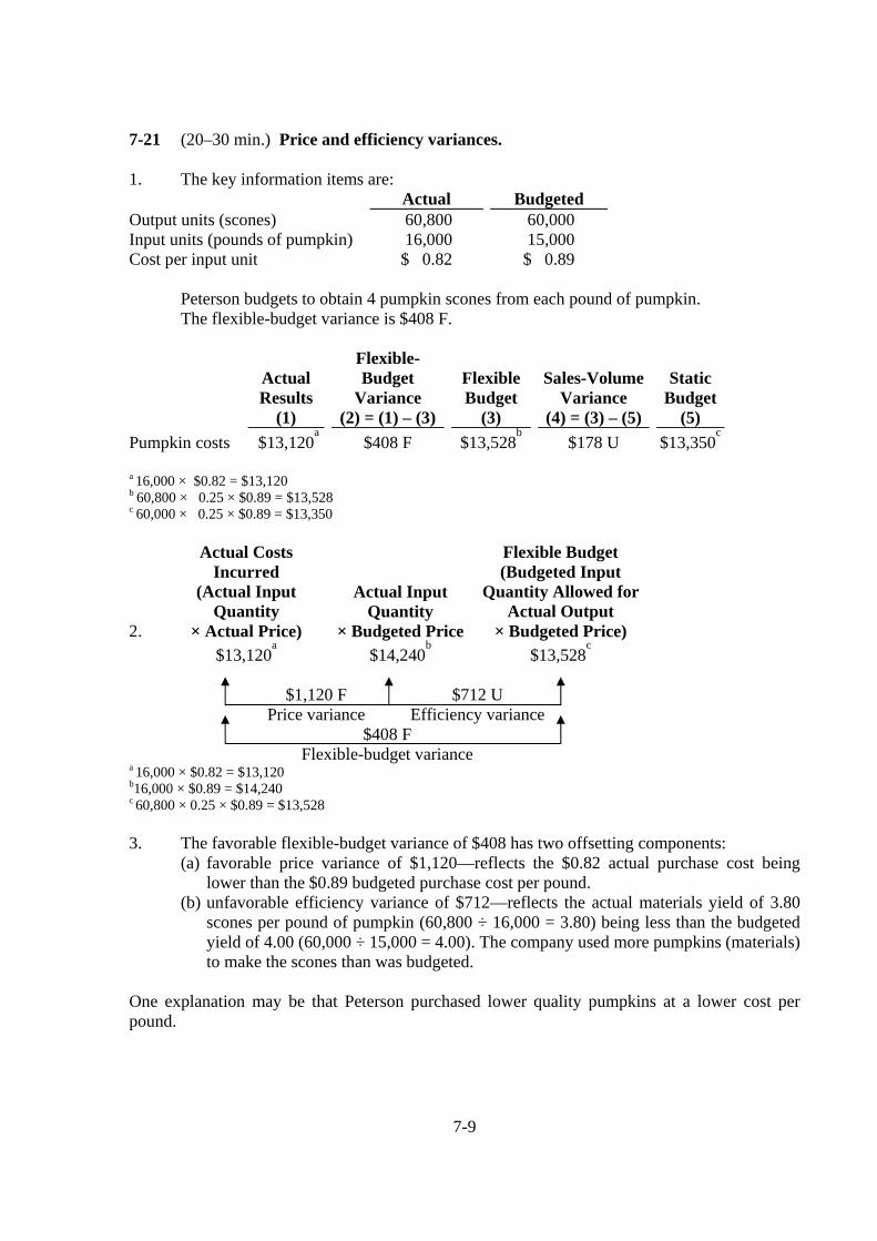
7-21 (20–30 min.) Price and efficiency variances. 1. The key information items are: Actual Budgeted Output units (scones) Input units (pounds of pumpkin) Cost per input unit

60,800 16,000 $ 0.82

60,000 15,000 $ 0.89

Peterson budgets to obtain 4 pumpkin scones from each pound of pumpkin. The flexible-budget variance is $408 F.

Actual Results

(1)

Flexible- Budget

Variance (2) = (1) – (3)

Flexible Budget

(3)

Sales-Volume

Variance (4) = (3) – (5)

Static

Budget (5)

Pumpkin costs $13,120a $408 F $13,528

b $178 U $13,350

c

a 16,000 × $0.82 = $13,120 b

60,800 × 0.25 × $0.89 = $13,528 c 60,000 × 0.25 × $0.89 = $13,350

2.

Actual Costs Incurred

(Actual Input Quantity

× Actual Price)

Actual Input Quantity

× Budgeted Price

Flexible Budget (Budgeted Input

Quantity Allowed for Actual Output

× Budgeted Price) $13,120

a $14,240

b $13,528

c

$1,120 F $712 U Price variance Efficiency variance $408 F Flexible-budget variance a 16,000 × $0.82 = $13,120

b16,000 × $0.89 = $14,240 c 60,800 × 0.25 × $0.89 = $13,528

3. The favorable flexible-budget variance of $408 has two offsetting components:

(a) favorable price variance of $1,120––reflects the $0.82 actual purchase cost being lower than the $0.89 budgeted purchase cost per pound.

(b) unfavorable efficiency variance of $712––reflects the actual materials yield of 3.80 scones per pound of pumpkin (60,800 ÷ 16,000 = 3.80) being less than the budgeted yield of 4.00 (60,000 ÷ 15,000 = 4.00). The company used more pumpkins (materials) to make the scones than was budgeted.

One explanation may be that Peterson purchased lower quality pumpkins at a lower cost per pound.

7-10

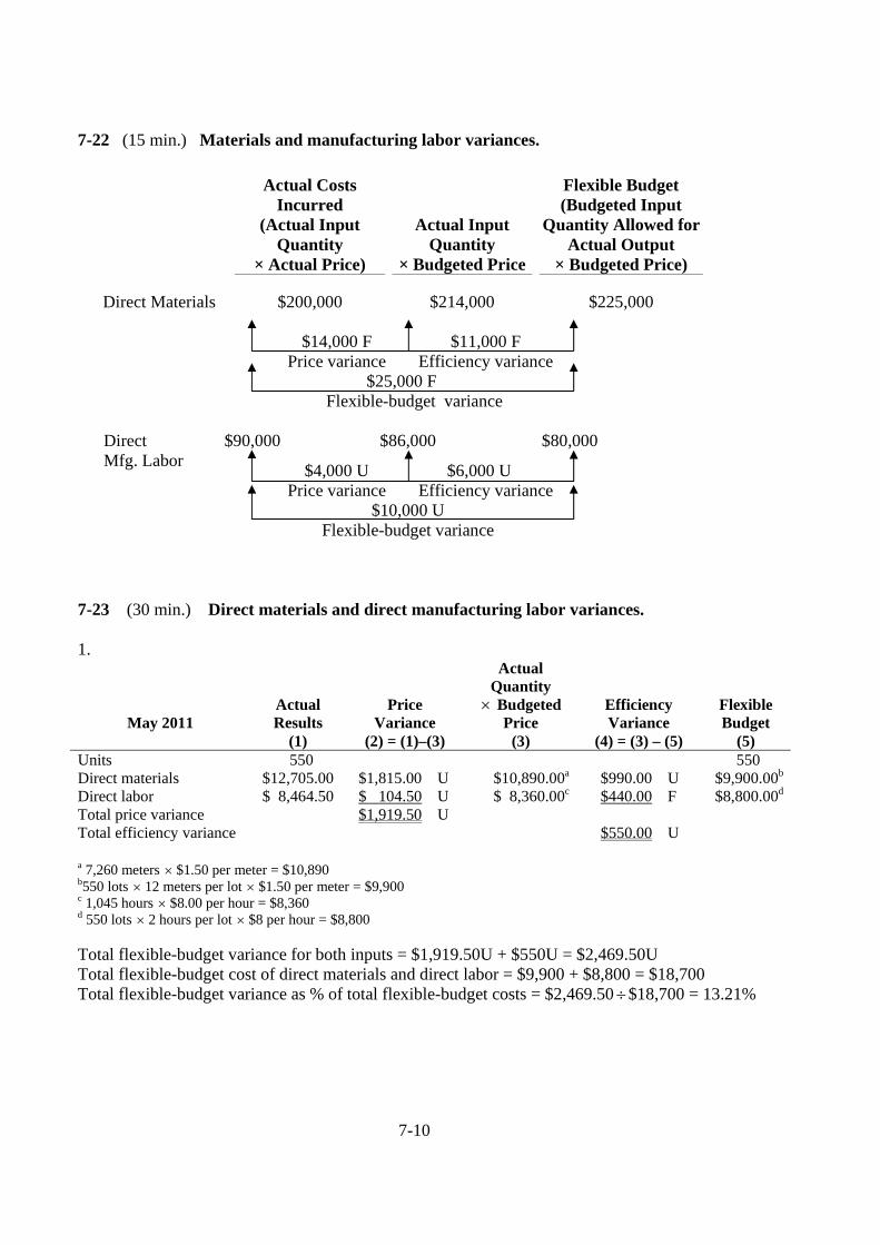
7-22 (15 min.) Materials and manufacturing labor variances.



× Actual Price)


× Budgeted Price



× Budgeted Price)

Direct Materials $200,000 $214,000 $225,000 $14,000 F $11,000 F Price variance Efficiency variance $25,000 F Flexible-budget variance Direct $90,000 $86,000 $80,000 Mfg. Labor $4,000 U $6,000 U Price variance Efficiency variance $10,000 U Flexible-budget variance 7-23 (30 min.) Direct materials and direct manufacturing labor variances. 1.

May 2011 Actual Results

Price Variance

Actual Quantity × Budgeted

Price Efficiency Variance

Flexible Budget

(1) (2) = (1)–(3) (3) (4) = (3) – (5) (5) Units 550 550 Direct materials $12,705.00 $1,815.00 U $10,890.00a $990.00 U $9,900.00b Direct labor $ 8,464.50 $ 104.50 U $ 8,360.00c $440.00 F $8,800.00d Total price variance $1,919.50 U Total efficiency variance $550.00 U

a 7,260 meters × $1.50 per meter = $10,890 b550 lots × 12 meters per lot × $1.50 per meter = $9,900 c 1,045 hours × $8.00 per hour = $8,360 d 550 lots × 2 hours per lot × $8 per hour = $8,800

Total flexible-budget variance for both inputs = $1,919.50U + $550U = $2,469.50U Total flexible-budget cost of direct materials and direct labor = $9,900 + $8,800 = $18,700 Total flexible-budget variance as % of total flexible-budget costs = $2,469.50÷$18,700 = 13.21%

7-11

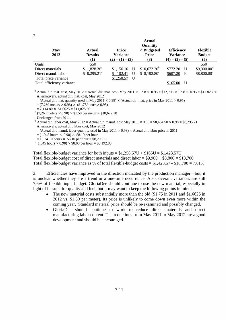
2.

May 2012

Actual Results

Price Variance

Actual Quantity × Budgeted


Flexible Budget

(1) (2) = (1) – (3) (3) (4) = (3) – (5) (5) Units 550 550 Direct materials $11,828.36a $1,156.16 U $10,672.20b $772.20 U $9,900.00c Direct manuf. labor $ 8,295.21d $ 102.41 U $ 8,192.80e $607.20 F $8,800.00c Total price variance $1,258.57 U Total efficiency variance $165.00 U a Actual dir. mat. cost, May 2012 = Actual dir. mat. cost, May 2011 × 0.98 × 0.95 = $12,705 × 0.98 × 0.95 = $11.828.36 Alternatively, actual dir. mat. cost, May 2012 = (Actual dir. mat. quantity used in May 2011 ×0.98) × (Actual dir. mat. price in May 2011 ×0.95) = (7,260 meters ×0.98) × ($1.75/meter ×0.95) = 7,114.80 × $1.6625 = $11,828.36 b (7,260 meters ×0.98) ×$1.50 per meter = $10,672.20 c Unchanged from 2011. d Actual dir. labor cost, May 2012 = Actual dir. manuf. cost May 2011 ×0.98 = $8,464.50 ×0.98 = $8,295.21 Alternatively, actual dir. labor cost, May 2012 = (Actual dir. manuf. labor quantity used in May 2011 ×0.98) ×Actual dir. labor price in 2011 = (1,045 hours × 0.98) × $8.10 per hour = 1,024.10 hours × $8.10 per hour = $8,295.21 e (1,045 hours ×0.98) ×$8.00 per hour = $8,192.80

Total flexible-budget variance for both inputs = $1,258.57U + $165U = $1,423.57U Total flexible-budget cost of direct materials and direct labor = $9,900 + $8,800 = $18,700 Total flexible-budget variance as % of total flexible-budget costs = $1,423.57÷$18,700 = 7.61% 3. Efficiencies have improved in the direction indicated by the production manager—but, it is unclear whether they are a trend or a one-time occurrence. Also, overall, variances are still 7.6% of flexible input budget. GloriaDee should continue to use the new material, especially in light of its superior quality and feel, but it may want to keep the following points in mind:

• The new material costs substantially more than the old ($1.75 in 2011 and $1.6625 in 2012 vs. $1.50 per meter). Its price is unlikely to come down even more within the coming year. Standard material price should be re-examined and possibly changed.

• GloriaDee should continue to work to reduce direct materials and direct manufacturing labor content. The reductions from May 2011 to May 2012 are a good development and should be encouraged.

7-12

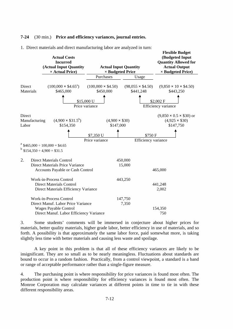
7-24 (30 min.) Price and efficiency variances, journal entries. 1. Direct materials and direct manufacturing labor are analyzed in turn:


(Actual Input Quantity × Actual Price)

Actual Input Quantity × Budgeted Price



× Budgeted Price) Direct Materials

(100,000 × $4.65a) $465,000

Purchases Usage (100,000 × $4.50) (98,055 × $4.50) $450,000 $441,248

(9,850 × 10 × $4.50) $443,250

$15,000 U $2,002 F Price variance Efficiency variance Direct Manufacturing Labor

(4,900 × $31.5b) $154,350

(4,900 × $30) $147,000

(9,850 × 0.5 × $30) or

(4,925 × $30) $147,750

$7,350 U $750 F Price variance Efficiency variance a $465,000 ÷ 100,000 = $4.65 b $154,350 ÷ 4,900 = $31.5 2. Direct Materials Control 450,000 Direct Materials Price Variance 15,000 Accounts Payable or Cash Control 465,000 Work-in-Process Control 443,250 Direct Materials Control 441,248 Direct Materials Efficiency Variance 2,002 Work-in-Process Control 147,750 Direct Manuf. Labor Price Variance 7,350 Wages Payable Control 154,350 Direct Manuf. Labor Efficiency Variance 750 3. Some students’ comments will be immersed in conjecture about higher prices for materials, better quality materials, higher grade labor, better efficiency in use of materials, and so forth. A possibility is that approximately the same labor force, paid somewhat more, is taking slightly less time with better materials and causing less waste and spoilage. A key point in this problem is that all of these efficiency variances are likely to be insignificant. They are so small as to be nearly meaningless. Fluctuations about standards are bound to occur in a random fashion. Practically, from a control viewpoint, a standard is a band or range of acceptable performance rather than a single-figure measure. 4. The purchasing point is where responsibility for price variances is found most often. The production point is where responsibility for efficiency variances is found most often. The Monroe Corporation may calculate variances at different points in time to tie in with these different responsibility areas.

7-13

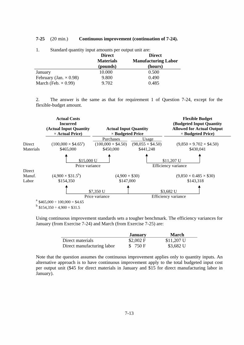
7-25 (20 min.) Continuous improvement (continuation of 7-24). 1. Standard quantity input amounts per output unit are: Direct

Materials (pounds)

Direct Manufacturing Labor

(hours) January February (Jan. × 0.98) March (Feb. × 0.99)

10.000 9.800 9.702

0.500 0.490 0.485

2. The answer is the same as that for requirement 1 of Question 7-24, except for the flexible-budget amount.


(Actual Input Quantity × Actual Price)


Flexible Budget (Budgeted Input Quantity Allowed for Actual Output


(100,000 × $4.65a)

$465,000

Purchases Usage (100,000 × $4.50) (98,055 × $4.50) $450,000 $441,248

(9,850 × 9.702 × $4.50)

$430,041

$15,000 U $11,207 U Price variance Efficiency variance

Direct Manuf. Labor

(4,900 × $31.5b)

$154,350

(4,900 × $30)

$147,000

(9,850 × 0.485 × $30)

$143,318 $7,350 U $3,682 U Price variance Efficiency variance a $465,000 ÷ 100,000 = $4.65 b $154,350 ÷ 4,900 = $31.5 Using continuous improvement standards sets a tougher benchmark. The efficiency variances for January (from Exercise 7-24) and March (from Exercise 7-25) are:

January March Direct materials Direct manufacturing labor

$2,002 F $ 750 F

$11,207 U $3,682 U

Note that the question assumes the continuous improvement applies only to quantity inputs. An alternative approach is to have continuous improvement apply to the total budgeted input cost per output unit ($45 for direct materials in January and $15 for direct manufacturing labor in January).

7-14

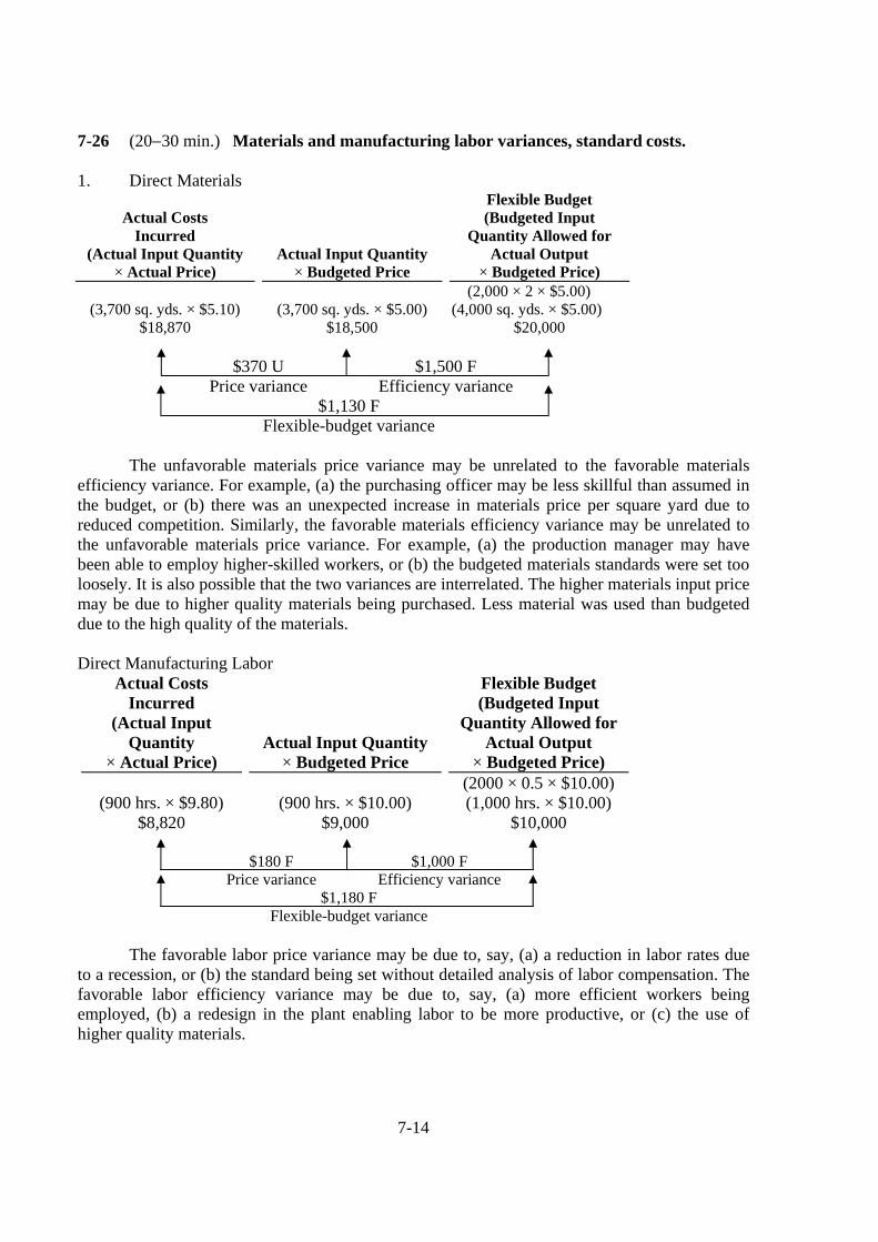
7-26 (20−30 min.) Materials and manufacturing labor variances, standard costs. 1. Direct Materials

Actual Costs

Incurred (Actual Input Quantity

× Actual Price)




× Budgeted Price)

(3,700 sq. yds. × $5.10) $18,870

(3,700 sq. yds. × $5.00)

$18,500

(2,000 × 2 × $5.00) (4,000 sq. yds. × $5.00)

$20,000 $370 U $1,500 F Price variance Efficiency variance $1,130 F Flexible-budget variance The unfavorable materials price variance may be unrelated to the favorable materials efficiency variance. For example, (a) the purchasing officer may be less skillful than assumed in the budget, or (b) there was an unexpected increase in materials price per square yard due to reduced competition. Similarly, the favorable materials efficiency variance may be unrelated to the unfavorable materials price variance. For example, (a) the production manager may have been able to employ higher-skilled workers, or (b) the budgeted materials standards were set too loosely. It is also possible that the two variances are interrelated. The higher materials input price may be due to higher quality materials being purchased. Less material was used than budgeted due to the high quality of the materials. Direct Manufacturing Labor



× Actual Price) Actual Input Quantity

× Budgeted Price



× Budgeted Price)

(900 hrs. × $9.80) $8,820

(900 hrs. × $10.00)

$9,000

(2000 × 0.5 × $10.00) (1,000 hrs. × $10.00)

$10,000 $180 F $1,000 F Price variance Efficiency variance $1,180 F Flexible-budget variance The favorable labor price variance may be due to, say, (a) a reduction in labor rates due to a recession, or (b) the standard being set without detailed analysis of labor compensation. The favorable labor efficiency variance may be due to, say, (a) more efficient workers being employed, (b) a redesign in the plant enabling labor to be more productive, or (c) the use of higher quality materials.

7-15

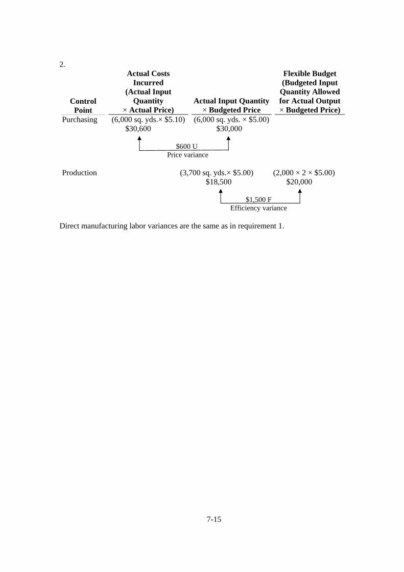
2.

Control Point



× Actual Price)

Actual Input Quantity× Budgeted Price


Quantity Allowed for Actual Output × Budgeted Price)

Purchasing (6,000 sq. yds.× $5.10) $30,600

(6,000 sq. yds. × $5.00) $30,000

$600 U Price variance Production (3,700 sq. yds.× $5.00)

$18,500 (2,000 × 2 × $5.00)

$20,000 $1,500 F Efficiency variance Direct manufacturing labor variances are the same as in requirement 1.

7-16

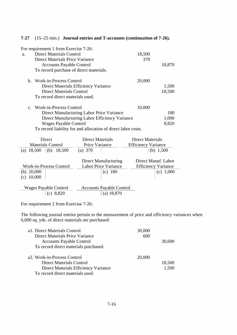
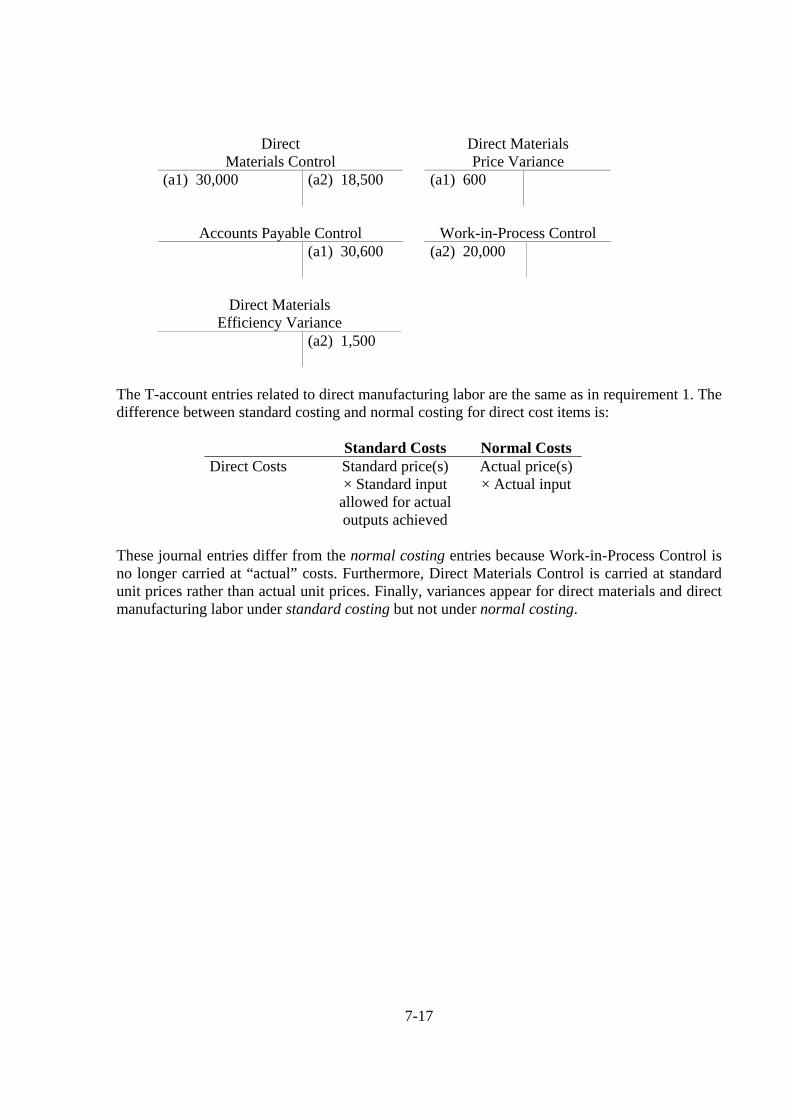
7-27 (15−25 min.) Journal entries and T-accounts (continuation of 7-26). For requirement 1 from Exercise 7-26: a. Direct Materials Control 18,500

Direct Materials Price Variance 370 Accounts Payable Control 18,870 To record purchase of direct materials. b. Work-in-Process Control 20,000 Direct Materials Efficiency Variance 1,500 Direct Materials Control 18,500 To record direct materials used. c. Work-in-Process Control 10,000 Direct Manufacturing Labor Price Variance 180 Direct Manufacturing Labor Efficiency Variance 1,000 Wages Payable Control 8,820 To record liability for and allocation of direct labor costs.

Direct

Materials Control Direct Materials

Price Variance Direct Materials

Efficiency Variance (a) 18,500 (b) 18,500 (a) 370 (b) 1,500

Work-in-Process Control

Direct Manufacturing Labor Price Variance

Direct Manuf. Labor Efficiency Variance

(b) 20,000 (c) 10,000

(c) 180 (c) 1,000

Wages Payable Control Accounts Payable Control

(c) 8,820 (a) 18,870 For requirement 2 from Exercise 7-26: The following journal entries pertain to the measurement of price and efficiency variances when 6,000 sq. yds. of direct materials are purchased:

a1. Direct Materials Control 30,000 Direct Materials Price Variance 600 Accounts Payable Control 30,600 To record direct materials purchased. a2. Work-in-Process Control 20,000 Direct Materials Control 18,500 Direct Materials Efficiency Variance 1,500 To record direct materials used.

7-17

Direct

Materials Control Direct Materials

Price Variance (a1) 30,000 (a2) 18,500

(a1) 600

Accounts Payable Control

Work-in-Process Control

(a1) 30,600

(a2) 20,000

Direct Materials

Efficiency Variance (a2) 1,500

The T-account entries related to direct manufacturing labor are the same as in requirement 1. The difference between standard costing and normal costing for direct cost items is:

Standard Costs Normal Costs Direct Costs Standard price(s)

× Standard input allowed for actual outputs achieved

Actual price(s) × Actual input

These journal entries differ from the normal costing entries because Work-in-Process Control is no longer carried at “actual” costs. Furthermore, Direct Materials Control is carried at standard unit prices rather than actual unit prices. Finally, variances appear for direct materials and direct manufacturing labor under standard costing but not under normal costing.

7-18

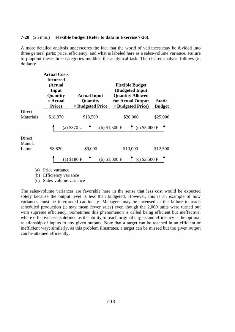
7-28 (25 min.) Flexible budget (Refer to data in Exercise 7-26). A more detailed analysis underscores the fact that the world of variances may be divided into three general parts: price, efficiency, and what is labeled here as a sales-volume variance. Failure to pinpoint these three categories muddies the analytical task. The clearer analysis follows (in dollars):

Actual Costs Incurred (Actual Input

Quantity × Actual

Price)


× Budgeted Price



Static Budget

Direct Materials

$18,870

$18,500

$20,000

$25,000

(a) $370 U (b) $1,500 F (c) $5,000 F Direct Manuf. Labor

$8,820

$9,000

$10,000

$12,500 (a) $180 F (b) $1,000 F (c) $2,500 F

(a) Price variance (b) Efficiency variance (c) Sales-volume variance

The sales-volume variances are favorable here in the sense that less cost would be expected solely because the output level is less than budgeted. However, this is an example of how variances must be interpreted cautiously. Managers may be incensed at the failure to reach scheduled production (it may mean fewer sales) even though the 2,000 units were turned out with supreme efficiency. Sometimes this phenomenon is called being efficient but ineffective, where effectiveness is defined as the ability to reach original targets and efficiency is the optimal relationship of inputs to any given outputs. Note that a target can be reached in an efficient or inefficient way; similarly, as this problem illustrates, a target can be missed but the given output can be attained efficiently.

7-19

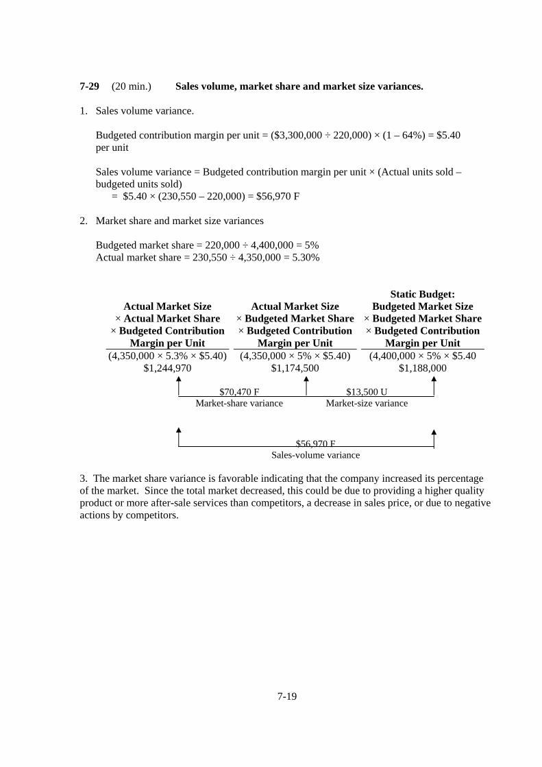
7-29 (20 min.) Sales volume, market share and market size variances. 1. Sales volume variance.

Budgeted contribution margin per unit = ($3,300,000 ÷ 220,000) × (1 – 64%) = $5.40 per unit Sales volume variance = Budgeted contribution margin per unit × (Actual units sold – budgeted units sold) = $5.40 × (230,550 – 220,000) = $56,970 F

2. Market share and market size variances Budgeted market share = 220,000 ÷ 4,400,000 = 5% Actual market share = 230,550 ÷ 4,350,000 = 5.30%

Actual Market Size


Margin per Unit

Actual Market Size


Margin per Unit



Margin per Unit (4,350,000 × 5.3% × $5.40)

$1,244,970 (4,350,000 × 5% × $5.40)

$1,174,500 (4,400,000 × 5% × $5.40

$1,188,000 $70,470 F $13,500 U Market-share variance Market-size variance

3. The market share variance is favorable indicating that the company increased its percentage of the market. Since the total market decreased, this could be due to providing a higher quality product or more after-sale services than competitors, a decrease in sales price, or due to negative actions by competitors.

$56,970 F Sales-volume variance

7-20

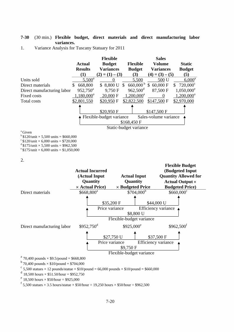
7-30 (30 min.) Flexible budget, direct materials and direct manufacturing labor variances.

1. Variance Analysis for Tuscany Statuary for 2011

Actual Results

(1)

Flexible Budget

Variances (2) = (1) – (3)

FlexibleBudget

(3)

Sales Volume

Variances (4) = (3) – (5)

Static Budget

(5) Units sold 5,500a 0 5,500 500 U 6,000a Direct materials $ 668,800 $ 8,800 U $ 660,000 b $ 60,000 F $ 720,000c Direct manufacturing labor 952,750a 9,750 F 962,500d 87,500 F 1,050,000e Fixed costs 1,180,000a 20,000 F 1,200,000a 0 1,200,000a Total costs $2,801,550 $20,950 F $2,822,500 $147,500 F $2,970,000 $20,950 F $147,500 F Flexible-budget variance Sales-volume variance $168,450 F

Static-budget variance a Given b $120/unit × 5,500 units = $660,000 c $120/unit × 6,000 units = $720,000 d $175/unit × 5,500 units = $962,500 e $175/unit × 6,000 units = $1,050,000 2.

Actual Incurred (Actual Input

Quantity × Actual Price)


× Budgeted Price



Direct materials $668,800a $704,000b $660,000c $35,200 F $44,000 U Price variance Efficiency variance $8,800 U Flexible-budget variance

Direct manufacturing labor $952,750d $925,000e $962,500f $27,750 U $37,500 F

Price variance Efficiency variance $9,750 F Flexible-budget variance a 70,400 pounds × $9.5/pound = $668,800 b 70,400 pounds × $10/pound = $704,000 c 5,500 statues × 12 pounds/statue × $10/pound = 66,000 pounds × $10/pound = $660,000 d 18,500 hours × $51.50/hour = $952,750 e 18,500 hours × $50/hour = $925,000 f 5,500 statues × 3.5 hours/statue × $50/hour = 19,250 hours × $50/hour = $962,500

7-21

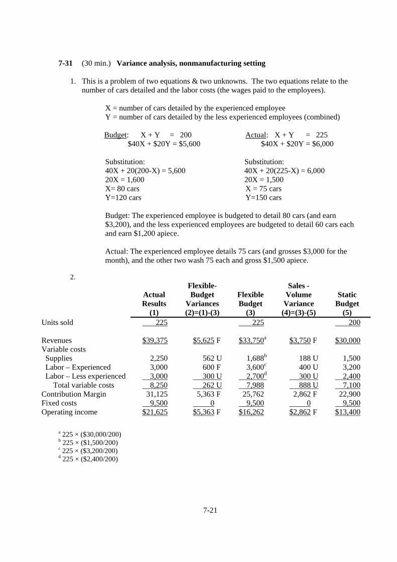
7-31 (30 min.) Variance analysis, nonmanufacturing setting

1. This is a problem of two equations & two unknowns. The two equations relate to the number of cars detailed and the labor costs (the wages paid to the employees).

X = number of cars detailed by the experienced employee Y = number of cars detailed by the less experienced employees (combined)

Budget: X + Y = 200 Actual: X + Y = 225 $40X + $20Y = $5,600 $40X + $20Y = $6,000

Substitution: Substitution: 40X + 20(200-X) = 5,600 40X + 20(225-X) = 6,000 20X = 1,600 20X = 1,500 X= 80 cars X = 75 cars Y=120 cars Y=150 cars

Budget: The experienced employee is budgeted to detail 80 cars (and earn $3,200), and the less experienced employees are budgeted to detail 60 cars each and earn $1,200 apiece.

Actual: The experienced employee details 75 cars (and grosses $3,000 for the month), and the other two wash 75 each and gross $1,500 apiece.

2.

Actual Results

(1)

Flexible- Budget

Variances (2)=(1)-(3)

Flexible Budget

(3)

Sales - Volume

Variance (4)=(3)-(5)

Static

Budget (5)

Units sold 225 225 200 Revenues $39,375 $5,625 F $33,750a $3,750 F $30,000 Variable costs Supplies 2,250 562 U 1,688b 188 U 1,500 Labor – Experienced 3,000 600 F 3,600c 400 U 3,200 Labor – Less experienced 3,000 300 U 2,700d 300 U 2,400 Total variable costs 8,250 262 U 7,988 888 U 7,100 Contribution Margin 31,125 5,363 F 25,762 2,862 F 22,900 Fixed costs 9,500 0 9,500 0 9,500 Operating income $21,625 $5,363 F $16,262 $2,862 F $13,400

a 225 × ($30,000/200) b 225 × ($1,500/200) c 225 × ($3,200/200) d 225 × ($2,400/200)

7-22

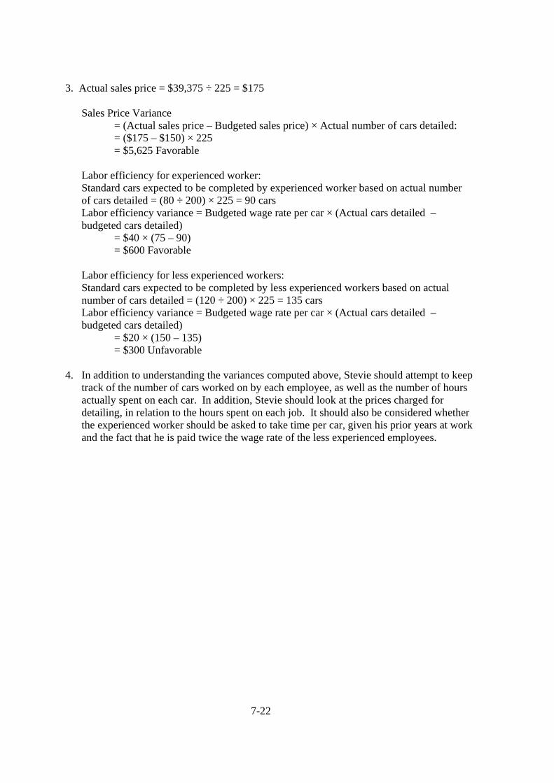
3. Actual sales price = $39,375 ÷ 225 = $175

Sales Price Variance = (Actual sales price – Budgeted sales price) × Actual number of cars detailed:

= ($175 – $150) × 225 = $5,625 Favorable Labor efficiency for experienced worker: Standard cars expected to be completed by experienced worker based on actual number

of cars detailed = (80 ÷ 200) × 225 = 90 cars Labor efficiency variance = Budgeted wage rate per car × (Actual cars detailed – budgeted cars detailed) = $40 × (75 – 90) = $600 Favorable

Labor efficiency for less experienced workers: Standard cars expected to be completed by less experienced workers based on actual

number of cars detailed = (120 ÷ 200) × 225 = 135 cars Labor efficiency variance = Budgeted wage rate per car × (Actual cars detailed – budgeted cars detailed) = $20 × (150 – 135) = $300 Unfavorable

4. In addition to understanding the variances computed above, Stevie should attempt to keep track of the number of cars worked on by each employee, as well as the number of hours actually spent on each car. In addition, Stevie should look at the prices charged for detailing, in relation to the hours spent on each job. It should also be considered whether the experienced worker should be asked to take time per car, given his prior years at work and the fact that he is paid twice the wage rate of the less experienced employees.

7-23

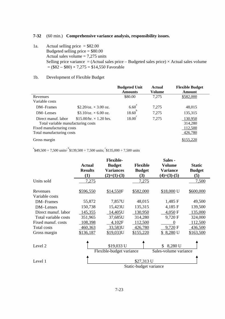
7-32 (60 min.) Comprehensive variance analysis, responsibility issues. 1a. Actual selling price = $82.00 Budgeted selling price = $80.00 Actual sales volume = 7,275 units Selling price variance = (Actual sales price − Budgeted sales price) × Actual sales volume = ($82 − $80) × 7,275 = $14,550 Favorable 1b. Development of Flexible Budget

Budgeted Unit

Amounts Actual Volume

Flexible Budget Amount

Revenues $80.00 7,275 $582,000 Variable costs DM−Frames $2.20/oz. × 3.00 oz. 6.60

a 7,275 48,015

DM−Lenses $3.10/oz. × 6.00 oz. 18.60b 7,275 135,315

Direct manuf. labor $15.00/hr. × 1.20 hrs. 18.00c 7,275 130,950

Total variable manufacturing costs 314,280 Fixed manufacturing costs 112,500 Total manufacturing costs 426,780

Gross margin $155,220 a$49,500 ÷ 7,500 units; b

$139,500 ÷ 7,500 units; c$135,000 ÷ 7,500 units

Actual Results

(1)

Flexible- Budget

Variances (2)=(1)-(3)

Flexible Budget

(3)

Sales - Volume

Variance (4)=(3)-(5)

Static

Budget (5)

Units sold 7,275 7,275 7,500 Revenues $596,550 $14,550F $582,000 $18,000 U $600,000 Variable costs DM−Frames 55,872 7,857U 48,015 1,485 F 49,500 DM−Lenses 150,738 15,423U 135,315 4,185 F 139,500 Direct manuf. labor 145,355 14,405U 130,950 4,050 F 135,000 Total variable costs 351,965 37,685U 314,280 9,720 F 324,000 Fixed manuf. costs 108,398 4,102F 112,500 0 112,500 Total costs 460,363 33,583U 426,780 9,720 F 436,500 Gross margin $136,187 $19,033U $155,220 $ 8,280 U $163,500

Level 2 $19,033 U $ 8,280 U Flexible-budget variance Sales-volume variance Level 1 $27,313 U Static-budget variance

7-24

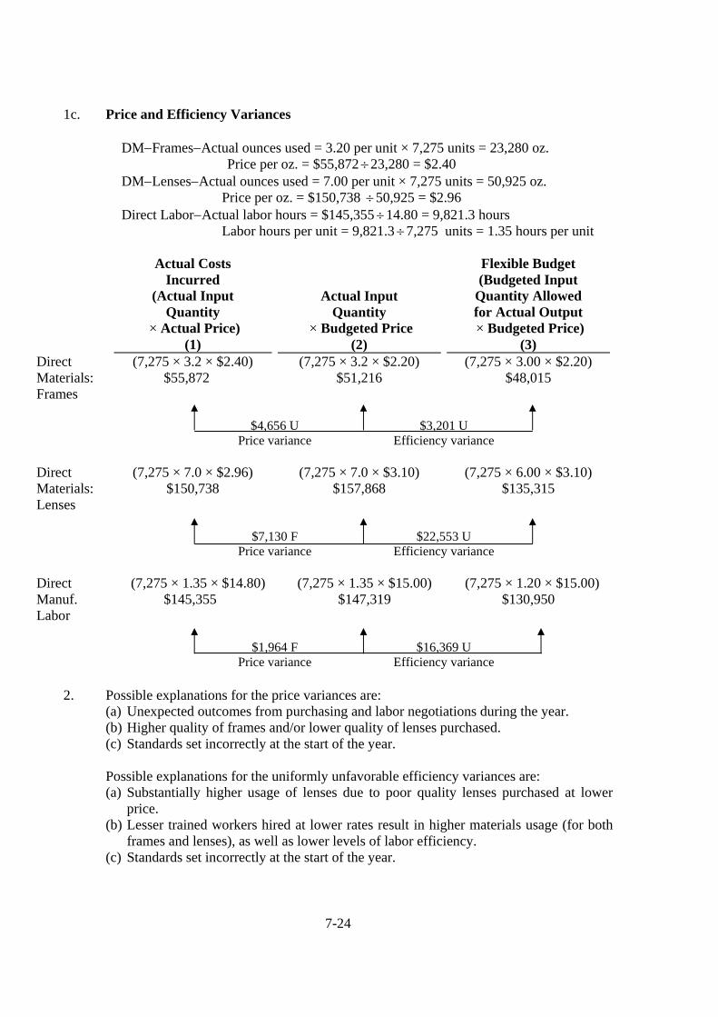
1c. Price and Efficiency Variances

DM−Frames−Actual ounces used = 3.20 per unit × 7,275 units = 23,280 oz. Price per oz. = $55,872÷23,280 = $2.40 DM−Lenses−Actual ounces used = 7.00 per unit × 7,275 units = 50,925 oz. Price per oz. = $150,738 ÷50,925 = $2.96 Direct Labor−Actual labor hours = $145,355÷14.80 = 9,821.3 hours Labor hours per unit = 9,821.3÷7,275 units = 1.35 hours per unit



× Actual Price) (1)


× Budgeted Price (2)



(3) Direct Materials: Frames

(7,275 × 3.2 × $2.40) $55,872

(7,275 × 3.2 × $2.20) $51,216

(7,275 × 3.00 × $2.20) $48,015


Direct Materials: Lenses

(7,275 × 7.0 × $2.96) $150,738

(7,275 × 7.0 × $3.10) $157,868

(7,275 × 6.00 × $3.10) $135,315

$7,130 F $22,553 U Price variance Efficiency variance

Direct Manuf. Labor

(7,275 × 1.35 × $14.80) $145,355

(7,275 × 1.35 × $15.00) $147,319

(7,275 × 1.20 × $15.00) $130,950

$1,964 F $16,369 U Price variance Efficiency variance 2. Possible explanations for the price variances are:

(a) Unexpected outcomes from purchasing and labor negotiations during the year. (b) Higher quality of frames and/or lower quality of lenses purchased. (c) Standards set incorrectly at the start of the year.

Possible explanations for the uniformly unfavorable efficiency variances are:

(a) Substantially higher usage of lenses due to poor quality lenses purchased at lower price.

(b) Lesser trained workers hired at lower rates result in higher materials usage (for both frames and lenses), as well as lower levels of labor efficiency.

(c) Standards set incorrectly at the start of the year.

7-25

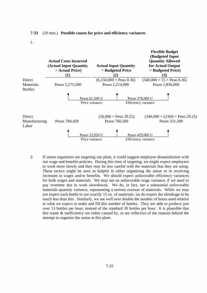
7-33 (20 min.) Possible causes for price and efficiency variances

1.

Actual Costs Incurred (Actual Input Quantity



(2)



(3) Direct Materials: Bottles

Pesos 2,275,500

(6,150,000 × Peso 0.36) Pesos 2,214,000

(340,000 × 15 × Peso 0.36) Pesos 1,836,000

Pesos 61,500 U Pesos 378,000 U Price variance Efficiency variance


Pesos 784,420

(26,000 × Peso 29.25) Pesos 760,500

(340,000 × (2/60) × Peso 29.25) Pesos 331,500

Pesos 23,920 U Pesos 429,000 U Price variance Efficiency variance 2. If union organizers are targeting our plant, it could suggest employee dissatisfaction with

our wage and benefits policies. During this time of targeting, we might expect employees to work more slowly and they may be less careful with the materials that they are using. These tactics might be seen as helpful in either organizing the union or in receiving increases in wages and/or benefits. We should expect unfavorable efficiency variances for both wages and materials. We may see an unfavorable wage variance, if we need to pay overtime due to work slowdowns. We do, in fact, see a substantial unfavorable materials quantity variance, representing a serious overuse of materials. While we may not expect each bottle to use exactly 15 oz. of materials, we do expect the shrinkage to be much less than this. Similarly, we see well over double the number of hours used relative to what we expect to make and fill this number of bottles. They are able to produce just over 13 bottles per hour, instead of the standard 30 bottles per hour. It is plausible that this waste & inefficiency are either caused by, or are reflective of the reasons behind the attempt to organize the union at this plant.

7-26

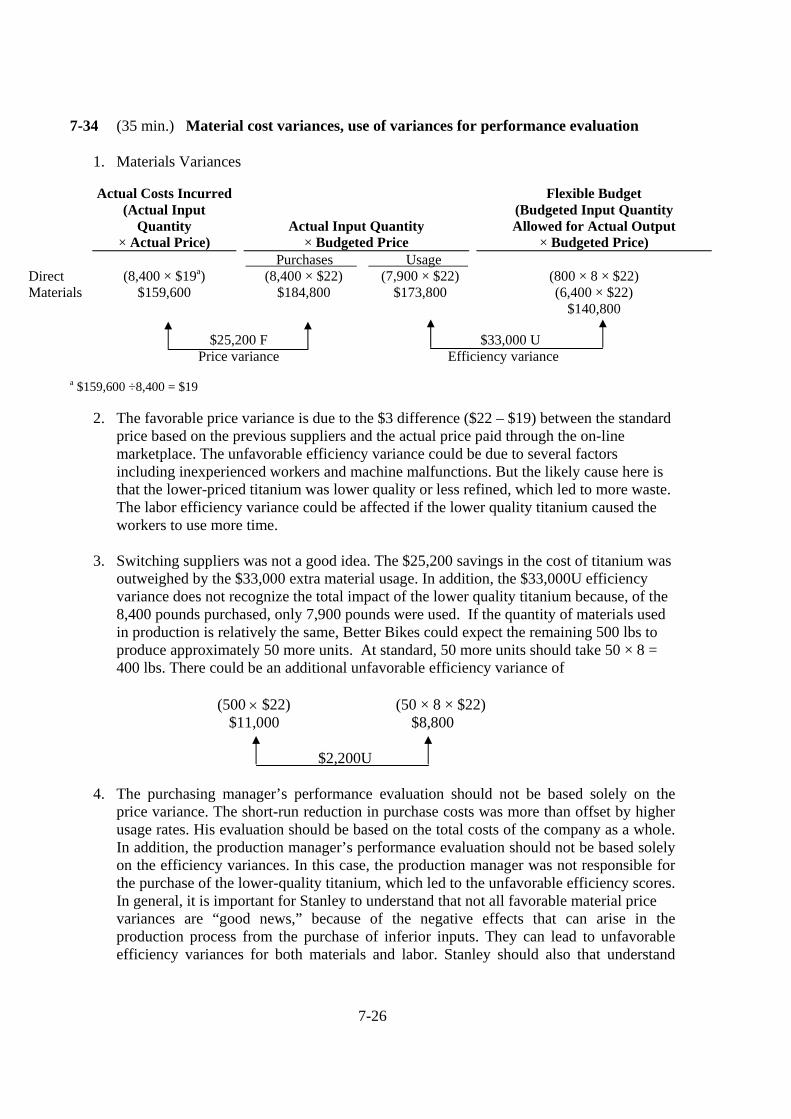
7-34 (35 min.) Material cost variances, use of variances for performance evaluation

1. Materials Variances

Actual Costs Incurred (Actual Input

Quantity × Actual Price)


Flexible Budget (Budgeted Input Quantity Allowed for Actual Output


(8,400 × $19a)

$159,600

Purchases Usage (8,400 × $22) (7,900 × $22) $184,800 $173,800

(800 × 8 × $22) (6,400 × $22)

$140,800

$25,200 F $33,000 U Price variance Efficiency variance a $159,600 ÷8,400 = $19

2. The favorable price variance is due to the $3 difference ($22 – $19) between the standard price based on the previous suppliers and the actual price paid through the on-line marketplace. The unfavorable efficiency variance could be due to several factors including inexperienced workers and machine malfunctions. But the likely cause here is that the lower-priced titanium was lower quality or less refined, which led to more waste. The labor efficiency variance could be affected if the lower quality titanium caused the workers to use more time.

3. Switching suppliers was not a good idea. The $25,200 savings in the cost of titanium was

outweighed by the $33,000 extra material usage. In addition, the $33,000U efficiency variance does not recognize the total impact of the lower quality titanium because, of the 8,400 pounds purchased, only 7,900 pounds were used. If the quantity of materials used in production is relatively the same, Better Bikes could expect the remaining 500 lbs to produce approximately 50 more units. At standard, 50 more units should take 50 × 8 = 400 lbs. There could be an additional unfavorable efficiency variance of (500 × $22) (50 × 8 × $22) $11,000 $8,800 $2,200U

4. The purchasing manager’s performance evaluation should not be based solely on the price variance. The short-run reduction in purchase costs was more than offset by higher usage rates. His evaluation should be based on the total costs of the company as a whole. In addition, the production manager’s performance evaluation should not be based solely on the efficiency variances. In this case, the production manager was not responsible for the purchase of the lower-quality titanium, which led to the unfavorable efficiency scores. In general, it is important for Stanley to understand that not all favorable material price variances are “good news,” because of the negative effects that can arise in the production process from the purchase of inferior inputs. They can lead to unfavorable efficiency variances for both materials and labor. Stanley should also that understand

7-27

efficiency variances may arise for many different reasons and she needs to know these reasons before evaluating performance.

5. Variances should be used to help Better Bikes understand what led to the current set of

financial results, as well as how to perform better in the future. They are a way to facilitate the continuous improvement efforts of the company. Rather than focusing solely on the price of titanium, Scott can balance price and quality in future purchase decisions.

6. Future problems can arise in the supply chain. Scott may need to go back to the previous

suppliers. But Better Bikes’ relationship with them may have been damaged and they may now be selling all their available titanium to other manufacturers. Lower quality bicycles could also affect Better Bikes’ reputation with the distributors, the bike shops and customers, leading to higher warranty claims and customer dissatisfaction, and decreased sales in the future.

7-28

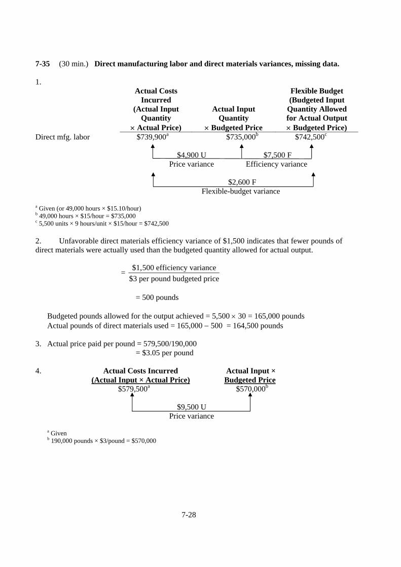
7-35 (30 min.) Direct manufacturing labor and direct materials variances, missing data. 1.



× Actual Price)


× Budgeted Price



Direct mfg. labor $739,900a $735,000b $742,500c $4,900 U $7,500 F Price variance Efficiency variance $2,600 F Flexible-budget variance a Given (or 49,000 hours × $15.10/hour) b 49,000 hours × $15/hour = $735,000 c 5,500 units × 9 hours/unit × $15/hour = $742,500

2. Unfavorable direct materials efficiency variance of $1,500 indicates that fewer pounds of direct materials were actually used than the budgeted quantity allowed for actual output.

= $1,500 efficiency variance$3 per pound budgeted price

= 500 pounds

Budgeted pounds allowed for the output achieved = 5,500 × 30 = 165,000 pounds Actual pounds of direct materials used = 165,000 − 500 = 164,500 pounds 3. Actual price paid per pound = 579,500/190,000 = $3.05 per pound 4. Actual Costs Incurred Actual Input × (Actual Input × Actual Price) Budgeted Price $579,500a $570,000b $9,500 U

Price variance

a Given b 190,000 pounds × $3/pound = $570,000

7-29

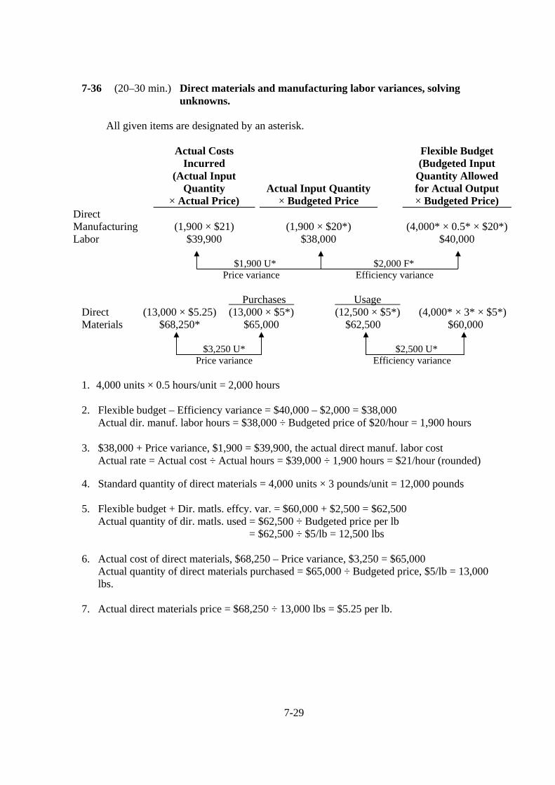
7-36 (20–30 min.) Direct materials and manufacturing labor variances, solving unknowns.

All given items are designated by an asterisk.







× Actual Price)

(1,900 × $21) $39,900

(1,900 × $20*)

$38,000

(4,000* × 0.5* × $20*)

$40,000 $1,900 U* $2,000 F* Price variance Efficiency variance

Purchases Usage Direct (13,000 × $5.25) (13,000 × $5*) (12,500 × $5*) (4,000* × 3* × $5*) Materials $68,250* $65,000 $62,500 $60,000 $3,250 U* $2,500 U* Price variance Efficiency variance 1. 4,000 units × 0.5 hours/unit = 2,000 hours 2. Flexible budget – Efficiency variance = $40,000 – $2,000 = $38,000

Actual dir. manuf. labor hours = $38,000 ÷ Budgeted price of $20/hour = 1,900 hours

3. $38,000 + Price variance, $1,900 = $39,900, the actual direct manuf. labor cost Actual rate = Actual cost ÷ Actual hours = $39,000 ÷ 1,900 hours = $21/hour (rounded)

4. Standard quantity of direct materials = 4,000 units × 3 pounds/unit = 12,000 pounds 5. Flexible budget + Dir. matls. effcy. var. = $60,000 + $2,500 = $62,500

Actual quantity of dir. matls. used = $62,500 ÷ Budgeted price per lb = $62,500 ÷ $5/lb = 12,500 lbs

6. Actual cost of direct materials, $68,250 – Price variance, $3,250 = $65,000 Actual quantity of direct materials purchased = $65,000 ÷ Budgeted price, $5/lb = 13,000 lbs.

7. Actual direct materials price = $68,250 ÷ 13,000 lbs = $5.25 per lb.

7-30

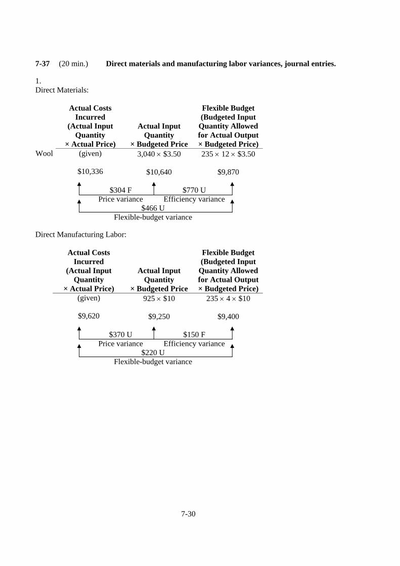
7-37 (20 min.) Direct materials and manufacturing labor variances, journal entries. 1. Direct Materials:



× Actual Price)


× Budgeted Price


Quantity Allowedfor Actual Output × Budgeted Price)

Wool (given)

$10,336

3,040 × $3.50

$10,640

235 × 12 × $3.50

$9,870 $304 F $770 U Price variance Efficiency variance $466 U Flexible-budget variance Direct Manufacturing Labor:



× Actual Price)


× Budgeted Price



(given)

$9,620

925 × $10

$9,250

235 × 4 × $10

$9,400 $370 U $150 F Price variance Efficiency variance $220 U Flexible-budget variance

7-31

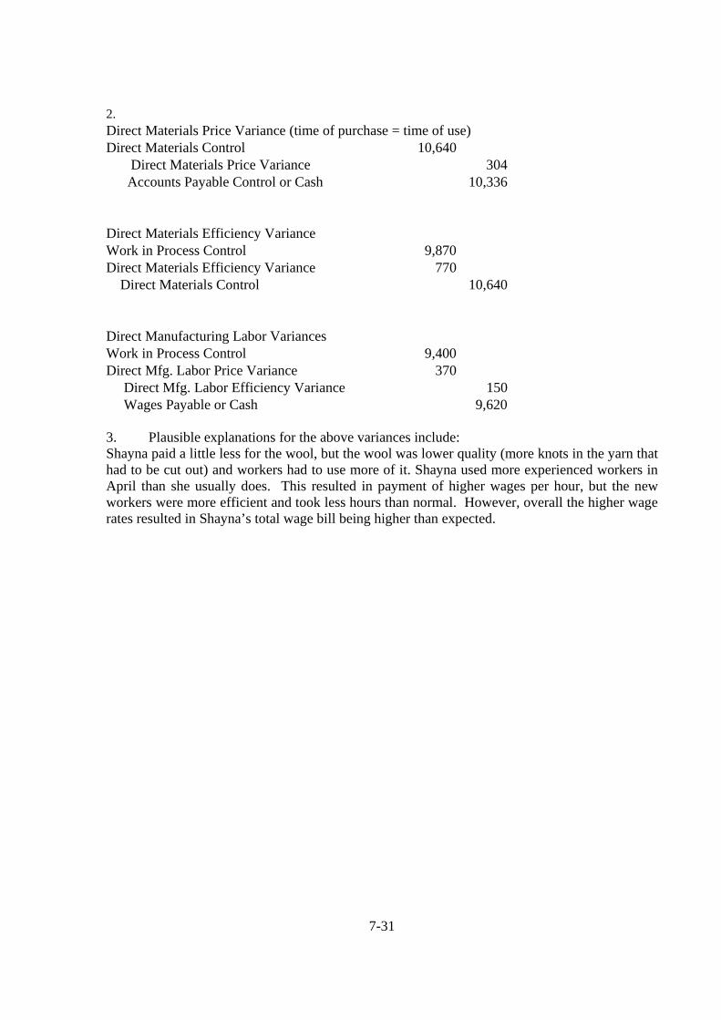
2. Direct Materials Price Variance (time of purchase = time of use) Direct Materials Control 10,640 Direct Materials Price Variance 304 Accounts Payable Control or Cash 10,336 Direct Materials Efficiency Variance Work in Process Control 9,870 Direct Materials Efficiency Variance 770 Direct Materials Control 10,640 Direct Manufacturing Labor Variances Work in Process Control 9,400 Direct Mfg. Labor Price Variance 370 Direct Mfg. Labor Efficiency Variance 150 Wages Payable or Cash 9,620 3. Plausible explanations for the above variances include: Shayna paid a little less for the wool, but the wool was lower quality (more knots in the yarn that had to be cut out) and workers had to use more of it. Shayna used more experienced workers in April than she usually does. This resulted in payment of higher wages per hour, but the new workers were more efficient and took less hours than normal. However, overall the higher wage rates resulted in Shayna’s total wage bill being higher than expected.

7-32

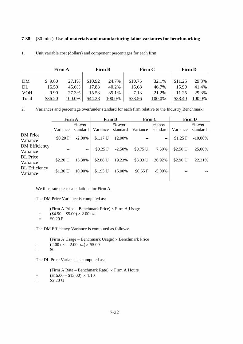
7-38 (30 min.) Use of materials and manufacturing labor variances for benchmarking. 1. Unit variable cost (dollars) and component percentages for each firm: Firm A Firm B Firm C Firm D DM $ 9.80 27.1% $10.92 24.7% $10.75 32.1% $11.25 29.3%DL 16.50 45.6% 17.83 40.2% 15.68 46.7% 15.90 41.4%VOH 9.90 27.3% 15.53 35.1% 7.13 21.2% 11.25 29.3%Total $36.20 100.0% $44.28 100.0% $33.56 100.0% $38.40 100.0% 2. Variances and percentage over/under standard for each firm relative to the Industry Benchmark: Firm A Firm B Firm C Firm D

Variance % over standard

Variance

% over standard

Variance

% over standard

Variance

% over standard

DM Price Variance $0.20 F -2.00% $1.17 U 12.00% -- -- $1.25 F -10.00%

DM Efficiency Variance -- -- $0.25 F -2.50% $0.75 U 7.50% $2.50 U 25.00%

DL Price Variance $2.20 U 15.38% $2.88 U 19.23% $3.33 U 26.92% $2.90 U 22.31%

DL Efficiency Variance $1.30 U 10.00% $1.95 U 15.00% $0.65 F -5.00% -- --

We illustrate these calculations for Firm A.

The DM Price Variance is computed as:

(Firm A Price – Benchmark Price) × Firm A Usage = ($4.90 – $5.00) × 2.00 oz. = $0.20 F

The DM Efficiency Variance is computed as follows:

(Firm A Usage – Benchmark Usage) × Benchmark Price

= (2.00 oz. – 2.00 oz.) × $5.00 = $0

The DL Price Variance is computed as:

(Firm A Rate – Benchmark Rate) × Firm A Hours

= ($15.00 – $13.00) × 1.10 = $2.20 U

7-33

The DL Efficiency Variance is computed as follows: (Firm A Usage – Benchmark Usage) × Benchmark Rate

= (1.10 hrs. – 1.00 hrs.) × $13.00 = $1.30 U

The % over standard is the percentage difference in prices relative to the Industry Benchmark. Again using the DM Price Variance calculation for Firm A, the % over standard is given by:

(Firm A Price – Benchmark Price) ÷ Benchmark Price = ($4.90 – $5.00) ÷ $5.00 = 2% under standard. 3. To: Boss From: Junior Accountant Re: Benchmarking & productivity improvements Date: March 15, 2011 Benchmarking advantages

– we can see how productive we are relative to our competition and the industry benchmark

– we can see the specific areas in which there may be opportunities for us to reduce costs Benchmarking disadvantages

– some of our competitors are targeting the market for high-end and custom-made lenses. I'm not sure that looking at their costs helps with understanding ours better

– we may focus too much on cost differentials and not enough on differentiating ourselves,

maintaining our competitive advantages, and growing our margins Areas to discuss

– we may want to find out whether we can get the same lower price for glass as Firm D

– we may want to re-evaluate the training our employees receive given our level of unfavorable labor efficiency variance compared to the benchmark.

– can we use Firm B’s materials efficiency and Firm C’s variable overhead consumption

levels as our standards for the coming year?

– It is unclear why the trade association is still using $13 for the labor rate benchmark. Given the difficulty of hiring qualified workers, real wage rates are now substantially higher. We pay our workers $2 more per hour, and our competitors pay even higher wages than we do!

7-34

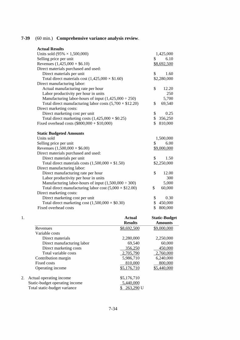
7-39 (60 min.) Comprehensive variance analysis review.

Actual Results Units sold (95% × 1,500,000) 1,425,000 Selling price per unit $ 6.10 Revenues (1,425,000 × $6.10) $8,692,500 Direct materials purchased and used: Direct materials per unit $ 1.60 Total direct materials cost (1,425,000 × $1.60) $2,280,000 Direct manufacturing labor: Actual manufacturing rate per hour $ 12.20 Labor productivity per hour in units 250 Manufacturing labor-hours of input (1,425,000 ÷ 250) 5,700 Total direct manufacturing labor costs (5,700 × $12.20) $ 69,540 Direct marketing costs: Direct marketing cost per unit $ 0.25 Total direct marketing costs (1,425,000 × $0.25) $ 356,250 Fixed overhead costs ($800,000 + $10,000) $ 810,000

Static Budgeted Amounts Units sold 1,500,000 Selling price per unit $ 6.00 Revenues (1,500,000 × $6.00) $9,000,000 Direct materials purchased and used:

Direct materials per unit $ 1.50 Total direct materials costs (1,500,000 × $1.50) $2,250,000 Direct manufacturing labor:

Direct manufacturing rate per hour $ 12.00 Labor productivity per hour in units 300 Manufacturing labor-hours of input (1,500,000 ÷ 300) 5,000 Total direct manufacturing labor cost (5,000 × $12.00) $ 60,000 Direct marketing costs: Direct marketing cost per unit $ 0.30 Total direct marketing cost (1,500,000 × $0.30) $ 450,000

Fixed overhead costs $ 800,000 1. Actual Static-Budget

Results Amounts Revenues $8,692,500 $9,000,000

Variable costs Direct materials 2,280,000 2,250,000 Direct manufacturing labor 69,540 60,000 Direct marketing costs 356,250 450,000 Total variable costs 2,705,790 2,760,000 Contribution margin 5,986,710 6,240,000 Fixed costs 810,000 800,000 Operating income $5,176,710 $5,440,000 2. Actual operating income $5,176,710 Static-budget operating income 5,440,000 Total static-budget variance $ 263,290 U

7-35

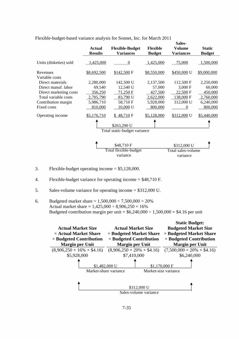
Flexible-budget-based variance analysis for Sonnet, Inc. for March 2011

Actual Results

Flexible-BudgetVariances

Flexible Budget

Sales-Volume

Variances

Static

Budget

Units (diskettes) sold 1,425,000 0 1,425,000 75,000 1,500,000 Revenues Variable costs Direct materials Direct manuf. labor Direct marketing costs Total variable costs

$8,692,500

2,280,000 69,540 356,250 2,705,790

$142,500 F

142,500 U 12,540 U 71,250 F 83,790 U

$8,550,000

2,137,500 57,000 427,500 2,622,000

$450,000 U

112,500 F 3,000 F 22,500 F 138,000 F

$9,000,000

2,250,000 60,000 450,000 2,760,000

Contribution margin 5,986,710 58,710 F 5,928,000 312,000 U 6,240,000Fixed costs 810,000 10,000 U 800,000 0 800,000

Operating income $5,176,710 $ 48,710 F $5,128,000 $312,000 U $5,440,000

3. Flexible-budget operating income = $5,128,000. 4. Flexible-budget variance for operating income = $48,710 F. 5. Sales-volume variance for operating income = $312,000 U. 6. Budgeted market share = 1,500,000 ÷ 7,500,000 = 20% Actual market share = 1,425,000 ÷ 8,906,250 = 16% Budgeted contribution margin per unit = $6,240,000 ÷ 1,500,000 = $4.16 per unit

Actual Market Size


Margin per Unit

Actual Market Size


Margin per Unit



Margin per Unit (8,906,250 × 16% × $4.16)

$5,928,000 (8,906,250 × 20% × $4.16)

$7,410,000 (7,500,000 × 20% × $4.16)

$6,240,000 $1,482,000 U $1,170,000 F Market-share variance Market-size variance

$312,000 U Total sales-volume

variance

$48,710 F Total flexible-budget

variance

$263,290 U Total static-budget variance

$312,000 U Sales-volume variance

7-36

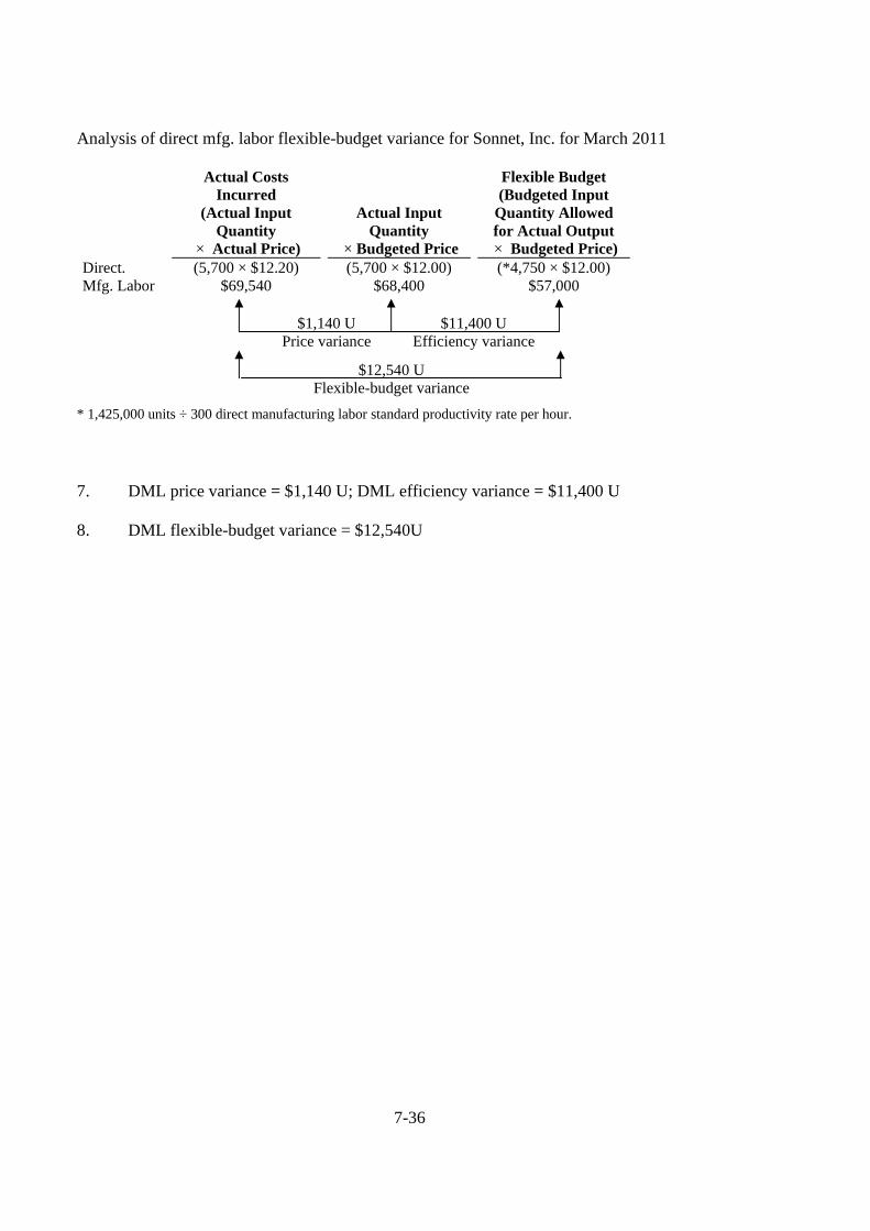
Analysis of direct mfg. labor flexible-budget variance for Sonnet, Inc. for March 2011



× Actual Price)


× Budgeted Price



Direct. Mfg. Labor

(5,700 × $12.20) $69,540

(5,700 × $12.00) $68,400

(*4,750 × $12.00) $57,000


* 1,425,000 units ÷ 300 direct manufacturing labor standard productivity rate per hour. 7. DML price variance = $1,140 U; DML efficiency variance = $11,400 U 8. DML flexible-budget variance = $12,540U

$12,540 U Flexible-budget variance

7-37

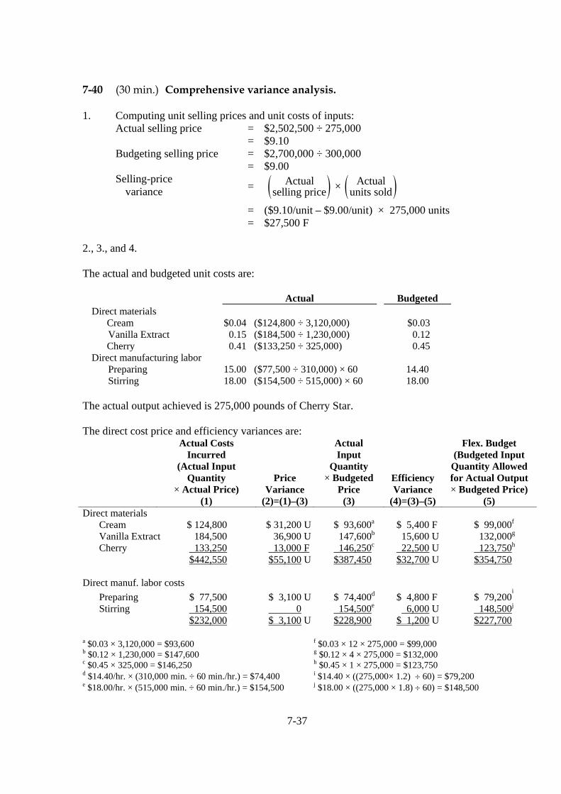
7-40 (30 min.) Comprehensive variance analysis. 1. Computing unit selling prices and unit costs of inputs:

Actual selling price = $2,502,500 ÷ 275,000 = $9.10 Budgeting selling price = $2,700,000 ÷ 300,000 = $9.00 Selling-price

variance = ( )Actualselling price × ( )Actual

units sold

= ($9.10/unit – $9.00/unit) × 275,000 units = $27,500 F

2., 3., and 4. The actual and budgeted unit costs are:

Actual Budgeted Direct materials Cream

Vanilla Extract Cherry

$0.04 ($124,800 ÷ 3,120,000) 0.15 ($184,500 ÷ 1,230,000) 0.41 ($133,250 ÷ 325,000)

$0.03 0.12 0.45

Direct manufacturing labor Preparing Stirring

15.00 ($77,500 ÷ 310,000) × 60 18.00 ($154,500 ÷ 515,000) × 60

14.40 18.00

The actual output achieved is 275,000 pounds of Cherry Star. The direct cost price and efficiency variances are:




Price Variance

(2)=(1)–(3)

Actual Input

Quantity × Budgeted

Price (3)

Efficiency Variance

(4)=(3)–(5)

Flex. Budget (Budgeted Input


(5) Direct materials

Cream $ 124,800 $ 31,200 U $ 93,600a $ 5,400 F $ 99,000f Vanilla Extract 184,500 36,900 U 147,600b 15,600 U 132,000g Cherry 133,250 13,000 F 146,250c 22,500 U 123,750h $442,550 $55,100 U $387,450 $32,700 U $354,750

Direct manuf. labor costs

Preparing $ 77,500 $ 3,100 U $ 74,400d $ 4,800 F $ 79,200i

Stirring 154,500 0 154,500e 6,000 U 148,500j $232,000 $ 3,100 U $228,900 $ 1,200 U $227,700

a $0.03 × 3,120,000 = $93,600

f $0.03 × 12 × 275,000 = $99,000 b $0.12 × 1,230,000 = $147,600

g $0.12 × 4 × 275,000 = $132,000 c $0.45 × 325,000 = $146,250

h $0.45 × 1 × 275,000 = $123,750 d $14.40/hr. × (310,000 min. ÷ 60 min./hr.) = $74,400

i $14.40 × ((275,000× 1.2) ÷ 60) = $79,200 e $18.00/hr. × (515,000 min. ÷ 60 min./hr.) = $154,500

j $18.00 × ((275,000 × 1.8) ÷ 60) = $148,500

7-38

Comments on the variances include

• Selling price variance. This may arise from a general increase in input prices (cream and vanilla). The sales price increase could be an effort to maintain a target margin. It could also arise from an overall industry increase in sales prices.

• Material price variance. The increase in the price per ounce of cream and vanilla extract could arise from uncontrollable market factors or from poor contract negotiations by Iceland. The decrease in the price per ounce of cherry could arise from good negotiations, a quantity discount or a lower quality input.

• Material efficiency variance. For vanilla extract and cherry, usage is greater than

budgeted. Possible reasons include lower quality inputs, use of lower quality workers, and the preparing and stirring equipment not being maintained in a fully operational mode. The favorable efficiency variance for cream could arise due to higher quality inputs (related to the unfavorable price variance) where less waste is experienced in the production process.

• Labor rate variance. The actual wage rate was higher for preparing than was

budgeted. This could arise due to hiring more experienced workers or unexpected overtime. The use of experienced workers is not supported by the material efficiency variance unless the machines are in very poor condition.

Labor efficiency variance. The favorable efficiency variance for preparing could be

due to workers eliminating nonvalue-added steps in production or more experienced workers being more efficient. The unfavorable efficiency variance for stirring could be due to inadequate training on new equipment or processes, or less experienced workers.

7-39

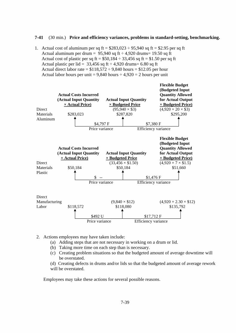
7-41 (30 min.) Price and efficiency variances, problems in standard-setting, benchmarking. 1. Actual cost of aluminum per sq ft = $283,023 ÷ 95,940 sq ft = $2.95 per sq ft

Actual aluminum per drum = 95,940 sq ft ÷ 4,920 drums= 19.50 sq ft Actual cost of plastic per sq ft = $50,184 ÷ 33,456 sq ft = $1.50 per sq ft Actual plastic per lid = 33,456 sq ft ÷ 4,920 drums= 6.80 sq ft Actual direct labor rate = $118,572 ÷ 9,840 hours = $12.05 per hour Actual labor hours per unit = 9,840 hours ÷ 4,920 = 2 hours per unit

Flexible Budget (Budgeted Input Actual Costs Incurred Quantity Allowed (Actual Input Quantity Actual Input Quantity for Actual Output × Actual Price) × Budgeted Price × Budgeted Price)

Direct (95,940 × $3) (4,920 × 20 × $3) Materials $283,023 $287,820 $295,200 Aluminum $4,797 F $7,380 F Price variance Efficiency variance

Flexible Budget (Budgeted Input Actual Costs Incurred Quantity Allowed (Actual Input Quantity Actual Input Quantity for Actual Output × Actual Price) × Budgeted Price × Budgeted Price)

Direct (33,456 × $1.50) (4,920 × 7 × $1.5) Materials $50,184 $50,184 $51,660 Plastic $ -- $1,476 F Price variance Efficiency variance Direct Manufacturing (9,840 × $12) (4,920 × 2.30 × $12) Labor $118,572 $118,080 $135,792 $492 U $17,712 F Price variance Efficiency variance 2. Actions employees may have taken include:

(a) Adding steps that are not necessary in working on a drum or lid. (b) Taking more time on each step than is necessary. (c) Creating problem situations so that the budgeted amount of average downtime will be overstated.

(d) Creating defects in drums and/or lids so that the budgeted amount of average rework will be overstated.

Employees may take these actions for several possible reasons.

7-40

(a) They may be paid on a piece-rate basis with incentives for production levels above budget.

(b) They may want to create a relaxed work atmosphere, and a less demanding standard can reduce stress.

(c) They have a “them vs. us” mentality rather than a partnership perspective. (d) They may want to gain all the benefits that ensue from superior performance (job

security, wage rate increases) without putting in the extra effort required.

This behavior is unethical if it is deliberately designed to undermine the credibility of the standards used at Stuckey.

3. If Jorgenson does nothing about standard costs, his behavior will violate the “Standards of Ethical Conduct for Practitioners of Management Accounting.” In particular, he would violate the (a) standards of competence, by not performing professional duties in accordance with

relevant standards; (b) standards of integrity, by passively subverting the attainment of the organization’s

objective to control costs; and (c) standards of credibility, by not communicating information fairly and not disclosing

all relevant cost information. 4. Jorgenson should discuss the situation with Fenton and point out that the standards are

lax and that this practice is unethical. If Fenton does not agree to change, Jorgenson should escalate the issue up the hierarchy in order to effect change. If organizational change is not forthcoming, Jorgenson should be prepared to resign rather than compromise his professional ethics.

5. Main pros of using Benchmarking Clearing House information to compute variances are:

(a) Highlights to Stuckey in a direct way how it may or may not be cost-competitive. (b) Provides a “reality check” to many internal positions about efficiency or

effectiveness. Main cons are:

(a) Stuckey may not be comparable to companies in the database. (b) Cost data about other companies may not be reliable. (c) Cost of Benchmarking Clearing House reports. Stuckey should be able to offset con #1 with a careful self-analysis of their firm to other firms. They can talk to the source to determine how reliable the information is.

7-41

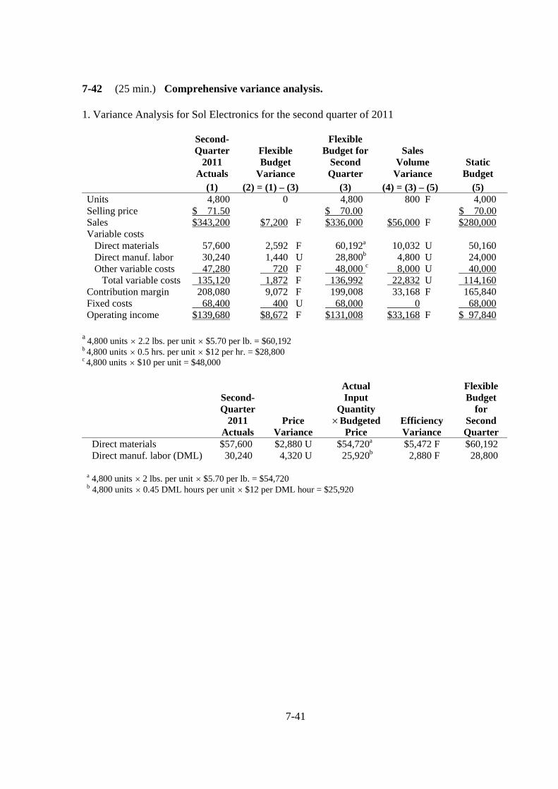
7-42 (25 min.) Comprehensive variance analysis. 1. Variance Analysis for Sol Electronics for the second quarter of 2011

Second-Quarter

2011 Actuals

Flexible Budget

Variance

Flexible Budget for

Second Quarter

Sales Volume

Variance Static

Budget (1) (2) = (1) – (3) (3) (4) = (3) – (5) (5) Units 4,800 0 4,800 800 F 4,000 Selling price $ 71.50 $ 70.00 $ 70.00 Sales $343,200 $7,200 F $336,000 $56,000 F $280,000 Variable costs Direct materials 57,600 2,592 F 60,192a 10,032 U 50,160 Direct manuf. labor 30,240 1,440 U 28,800b 4,800 U 24,000 Other variable costs 47,280 720 F 48,000 c 8,000 U 40,000 Total variable costs 135,120 1,872 F 136,992 22,832 U 114,160 Contribution margin 208,080 9,072 F 199,008 33,168 F 165,840 Fixed costs 68,400 400 U 68,000 0 68,000 Operating income $139,680 $8,672 F $131,008 $33,168 F $ 97,840

a 4,800 units × 2.2 lbs. per unit × $5.70 per lb. = $60,192 b 4,800 units × 0.5 hrs. per unit × $12 per hr. = $28,800 c 4,800 units × $10 per unit = $48,000

Second-Quarter

2011 Actuals

Price Variance

Actual Input

Quantity ×Budgeted


Flexible Budget

for Second Quarter

Direct materials $57,600 $2,880 U $54,720a $5,472 F $60,192 Direct manuf. labor (DML) 30,240 4,320 U 25,920b 2,880 F 28,800 a 4,800 units × 2 lbs. per unit × $5.70 per lb. = $54,720 b 4,800 units × 0.45 DML hours per unit × $12 per DML hour = $25,920

7-42

2 The following details, revealed in the variance analysis, should be used to rebut the union if it focuses on the favorable operating income variance:

• Most of the static budget operating income variance of $41,840F ($139,680 – $97,840) comes from a favorable sales volume variance, which only arose because Sol sold more units than planned.

• Of the $8,672 F flexible-budget variance in operating income, most of it comes from the $7,200F flexible-budget variance in sales.

• The net flexible-budget variance in total variable costs of $1,872 F is small, and it arises from direct materials and other variable costs, not from labor. Direct manufacturing labor flexible-budget variance is $1,440 U.

• The direct manufacturing labor price variance, $4,320U, which is large and unfavorable, is indeed offset by direct manufacturing labor’s favorable efficiency variance—but the efficiency variance is driven by the fact that Sol is using new, more expensive materials. Shaw may have to “prove” this to the union which will insist that it’s because workers are working smarter. Even if workers are working smarter, the favorable direct manufacturing labor efficiency variance of $2,880 does not offset the unfavorable direct manufacturing labor price variance of $4,320.

3. Changing the standards may make them more realistic, making it easier to negotiate with the union. But the union will resist any tightening of labor standards, and it may be too early (is one quarter’s experience enough to change on?); a change of standards at this point may be viewed as opportunistic by the union. Perhaps a continuous improvement program to change the standards will be more palatable to the union and will achieve the same result over a somewhat longer period of time.

Documents

CHAPTER 7 FLEXIBLE BUDGETS, DIRECT-COST … 7 FLEXIBLE BUDGETS, DIRECT-COST VARIANCES, AND MANAGEMENT CONTROL ... cost management, (ii) pricing decisions,