Embed Size (px)
DESCRIPTION
''''
Citation preview

Agricultural Economics Research Review
ISSN 0971-3441Online ISSN 0974-0279
Agricultural Economics Research Association (India)
Regd. No. F2 (A/67)/89
Agricultural Economics Research Association (India), a registered society which came into being in 1987, has on date more than 745 life members, 110 ordinary members, more than 115 institutional members and 25 honorary life members from India and abroad. The mandate of the Association is to promote the study of agricultural economics in particular and socio-economic problems in general. The Association has been regularly publishing a six-monthly research Journal “Agricultural Economics Research Review” since 1988. Besides refereed research articles, comprehensive review articles in the area of agricultural economics (including horticulture and fisheries), conference/symposia proceedings and book reviews are also published in the Journal. To encourage the young researchers, abstracts of M.Sc. and Ph.D. theses in agricultural economics are also published in the Journal. The Association has been successfully organizing national conferences regularly on topical policy issues, the proceedings of which have been published. The Association undertakes sponsored research studies. Over the years, the Association has attained a wide visibility and professional credibility. The official journal of the Association, namely, Agricultural Economics Research Review has been highly rated by National Academy of Agricultural Science, New Delhi.
Address for Correspondence:SecretaryAgricultural Economics Research Association (India)F-4, A Block, National Agricultural Science Centre (NASC) ComplexDev Prakash Shastri Marg, PusaNew Delhi 110 012, India
Email: [email protected]: www.aeraindia.in
Agricultural Economics Research Association (India)
About the Association
Printed at Cambridge Printing Works, B-85, Naraina Industrial Area, Phase-II, New Delhi - 110 028.
July-December2013Volume 26Number 2
V.P.S. ARORA: Agricultural Policies in India: Retrospect and Prospect
SURESH C. BABU , P.K. JOSHI, CLAIRE J. GLENDENNING, KWADWO ASENSO-OKYERE AND RASHEED SULAIMAN V.: The State of Agricultural Extension Reforms in India: Strategic Priorities and Policy Options
RASHMI AGRAWAL, S.K. NANDA, D. RAMA RAO AND B.V.L.N. RAO: Integrated Approach to Human Resource Forecasting: An Exercise in Agricultural Sector
LIJO THOMAS, GIRISH KUMAR JHA AND SURESH PAL: External Market Linkages and Instability in Indian Edible Oil Economy: Implications for Self-sufficiency Policy in Edible Oils
ELUMALAI KANNAN: Does Decentralization Improve Agricultural Services Delivery? — Evidence from Karnataka
ANJANI KUMAR, SHINOJ PARAPPURATHU AND P.K. JOSHI: Structural Transformation in Dairy Sector of India
HARI KRISHNA SHRESTHA, HIRA KAJI MANANDHAR AND PUNYA PRASAD REGMI: Investment in Wheat Research in Nepal – An Empirical Analysis
GIRISH K. JHA AND KANCHAN SINHA: Agricultural Price Forecasting Using Neural Network Model: An Innovative Information Delivery System
AKHTER ALI: Farmers’ Willingness to Pay for Index Based Crop Insurance in Pakistan: A Case Study on Food and Cash Crops of Rain-fed Areas
RANJIT KUMAR PAUL, SANJEEV PANWAR, SUSHEEL KUMAR SARKAR, ANIL KUMAR, K.N. SINGH, SAMIR FAROOQI AND VIPIN KUMAR CHOUDHARY: Modelling and Forecasting of Meat Exports from India
PAVITHRA S. AND KAMAL VATTA: Role of Non-Farm Sector in Sustaining Rural Livelihoods in Punjab
Y. LATIKA DEVI, JASDEV SINGH, KAMAL VATTA AND SANJAY KUMAR: Dynamics of Labour Demand and its Determinants in Punjab Agriculture
A.N. SHUKLA, S.K. TEWARI AND P.P. DUBEY: Factors Affecting Profitability of Commercial Banks: A Rural Perspective
AJMER SINGH, RAJBIR YADAV AND SATYAVIR SINGH: Exploring Possibilities of Extending Wheat Cultivation to Newer Areas: A Study on Economic Feasibility of Wheat Production in Southern Hills Zone of India
VINOD KUMAR VERMA, VISHNU SHANKER MEENA, PRADEEP KUMAR AND R.C. KUMAWAT: Production and Marketing of Cumin in Jodhpur District of Rajasthan: An Economic Analysis
D.K. GROVER AND J.M. SINGH: Post-harvest Losses in Wheat Crop in Punjab: Past and Present
AG
RIC
ULT
UR
AL
EC
ON
OM
ICS
RE
SE
AR
CH
RE
VIE
W Vo
l. 26 (2) July-D
ecemb
er 2013
se eR a s rcci h m Ao sn so oc ciE a l ta ior nut l (Iu nci dr iag )A

AGRICULTURAL ECONOMICS RESEARCH REVIEW
EDITORIAL BOARD
Chairman : Dr. S.S. Acharya, Honorary Professor, IDS, 33, Shahi Complex, Sector 11,Udaipur – 313 002 (Rajasthan)
Chief Editor : Dr. Ramesh Chand, Director, National Centre for Agricultural Economics and PolicyResearch, Pusa, New Delhi – 110 012
Managing Editor : Dr. Pratap S. Birthal, Principal Scientist, National Centre for Agricultural Economicsand Policy Research, Pusa, New Delhi – 110 012
Members : Dr. J.R. Anderson, Emeritus Professor of Agricultural Economics, University ofNew England, Armidale (Australia)
Dr. Derek Byerlee, Member, Independent Science and Partnership Council, CGIAR,c/o FAO, Rome (Italy)
Dr. R. S. Deshpande, Director, Institute for Social and Economic Change,Nagarabhavi P.O., Bangalore – 560 072 (Karnataka)
Dr. Madhur Gautam, Lead Economist, The World Bank, Washinton DC 20433(USA)
Dr. Kisan Gunjal, Economist, Food and Agriculture Organization of the UnitedNations (FAO), Rome (Italy)
Dr. Girish K. Jha, Division of Agricultural Economics, Indian Agricultural ResearchInstitute, New Delhi – 110 012
Dr. P.K. Joshi, Director–South Asia, International Food Policy Research Institute,NASC Complex, Dev Prakash Shastri Marg, New Delhi – 110 012
Dr. M. Krishnan, Principal Scientist and Head, Division of Fisheries Economics,Extension and Statistics, Central Institute of Fisheries Education, Versova, Andheri(W), Mumbai – 400 061 (Maharashtra)
Dr. Surabhi Mittal, Senior Scientist, CIMMYT-India, NASC Complex, DPS Marg,New Delhi – 110 012
Dr. S. Mohanty, Head (Social Sciences), International Rice Research Institute,Manila (Philippines)
Dr. K. Palanisami, Director, IWMI-TATA Policy Research Program, InternationalCrops Research Institute for the Semi-Arid Tropics, Patancheru – 502 324(Andhra Pradesh)
Dr. P. Parthasarthy Rao, Principal Scientist (Economics) and Assistant ResearchProgram Director, RP-Markets, Institutions & Policies, International Crops ResearchInstitute for the Semi-Arid Tropics (ICRISAT), Patancheru – 502 324 (AndhraPradesh)
Dr. R.S. Sidhu, Dean, College of Basic Sciences and Humanities, PunjabAgricultural University, Ludhiana – 141 004 (Punjab)
Dr. H.S. Vijaya Kumar, Professor, Deptt. of Agril. Marketing, Cooperation andAgribusiness Management, College of Agriculture, Dharwad – 580 005 (Karnataka)

ISSN 0971-3441Online ISSN 0974-0279
Agricultural Economics Research Review
Agricultural Economics Research Association (India)National Agricultural Science Centre Complex
Dev Prakash Shastri Marg, PusaNew Delhi - 110 012

Agricultural Economics Research ReviewVol. 26 (No.2) July-December 2013
© Agricultural Economics Research Association (India) 2013
Financial support from:Indian Council of Agricultural Research (ICAR), New Delhi
Published by:Dr Suresh Pal, Secretary, AERA on behalf of Agricultural Economics Research Association (India)
Printed at:Cambridge Printing Works, B-85, Phase II, Naraina Industrial Area, New Delhi 110 028

ISSN 0971-3441
Agricultural Economics Research Review[Journal of the Agricultural Economics Research Association (India)]
Volume 26 Number 2 July-December 2013
CONTENTS
Agricultural Policies in India: Retrospect and Prospect 135V.P.S. Arora
The State of Agricultural Extension Reforms in India: Strategic Priorities and Policy Options 159Suresh C. Babu , P.K. Joshi, Claire J. Glendenning, Kwadwo Asenso-Okyereand Rasheed Sulaiman V.
Integrated Approach to Human Resource Forecasting: An Exercise in Agricultural Sector 173Rashmi Agrawal, S.K. Nanda, D. Rama Rao and B.V.L.N. Rao
External Market Linkages and Instability in Indian Edible Oil Economy: Implications for 185Self-sufficiency Policy in Edible Oils
Lijo Thomas, Girish Kumar Jha and Suresh Pal
Does Decentralization Improve Agricultural Services Delivery? — Evidence from Karnataka 199Elumalai Kannan
Structural Transformation in Dairy Sector of India 209Anjani Kumar, Shinoj Parappurathu and P.K. Joshi
Investment in Wheat Research in Nepal – An Empirical Analysis 221Hari Krishna Shrestha, Hira Kaji Manandhar and Punya Prasad Regmi
Agricultural Price Forecasting Using Neural Network Model: An Innovative Information 229Delivery System
Girish K. Jha and Kanchan Sinha
Farmers’ Willingness to Pay for Index Based Crop Insurance in Pakistan: A Case Study on Food 241and Cash Crops of Rain-fed Areas
Akhter Ali
Modelling and Forecasting of Meat Exports from India 249Ranjit Kumar Paul, Sanjeev Panwar, Susheel Kumar Sarkar, Anil Kumar, K.N. Singh,Samir Farooqi and Vipin Kumar Choudhary
Role of Non-Farm Sector in Sustaining Rural Livelihoods in Punjab 257Pavithra S. and Kamal Vatta
Contd....

Contents contd....Dynamics of Labour Demand and its Determinants in Punjab Agriculture 267
Y. Latika Devi, Jasdev Singh, Kamal Vatta and Sanjay Kumar
Research NotesFactors Affecting Profitability of Commercial Banks: A Rural Perspective 275
A.N. Shukla, S.K. Tewari and P.P. Dubey
Exploring Possibilities of Extending Wheat Cultivation to Newer Areas: A Study on Economic 281Feasibility of Wheat Production in Southern Hills Zone of India
Ajmer Singh, Rajbir Yadav and Satyavir Singh
Production and Marketing of Cumin in Jodhpur District of Rajasthan: An Economic Analysis 287Vinod Kumar Verma, Vishnu Shanker Meena, Pradeep Kumar and R.C. Kumawat
Post-harvest Losses in Wheat Crop in Punjab: Past and Present 293D.K. Grover and J.M. Singh
Abstracts of M.Sc. Theses 299
Abstracts of Ph.D. Theses 303
Book Review 305
Guidelines for Submission of Papers/Abstracts 307
Author Index
Agrawal, Rashmi 173Ali, Akhter 241Arora, V.P.S. 135Asenso-Okyere, Kwadwo 159Babu, Suresh C. 159Choudhary, Vipin Kumar 249Dubey, P.P. 275Farooqi, Samir 249Glendenning, Claire J. 159Grover, D.K. 293Jha, Girish K. 185, 229Joshi, P.K. 159, 209Kannan, Elumalai 199Kumar, Anil 249Kumar, Anjani 209
Kumar, Pradeep 287Kumar, Sanjay 267Kumawat, R.C. 287Latika Devi, Y. 267Manandhar, Hira Kaji 221Meena, Vishnu Shanker 287Nanda, S.K. 173Pal, Suresh 185Panwar, Sanjeev 249Parappurathu, Shinoj 209Paul, Ranjit Kumar 249Pavithra, S. 257Rama Rao, D. 173Rao, B.V.L.N. 173Regmi, Punya Prasad 221
Sarkar, Susheel Kumar 249Shrestha, Hari Krishna 221Shukla, A.N. 275Singh, Ajmer 281Singh, J.M. 293Singh, Jasdev 267Singh, K.N. 249Singh, Satyavir 281Sinha, Kanchan 229Sulaiman V., Rasheed 159Tewari, S.K. 275Thomas, Lijo 185Vatta, Kamal 257, 267Verma, Vinod Kumar 287Yadav, Rajbir 281

Agricultural Economics Research ReviewVol. 26 (No.2) July-December 2013 pp 135-157
Agricultural Policies in India: Retrospect and Prospect§
V.P.S. AroraVice-Chancellor, Supertech University, Rudrapur, Uttarakhand
Agriculture continues to be an important sector ofIndian economy, though its share in the gross domesticproduct (GDP) has declined from about 50 per cent inearly-1950s to 14 per cent in 2011-12. Employment inagriculture has also shown a decline, albeit slowly, andpresently it accounts for 52 per cent of the country’stotal labour force. The declining share of agriculturein GDP and employment is consistent with the theoryof economic development. However, a faster andsustainable growth in the sector remains vital forcreation of jobs, enhancing incomes, and ensuring foodsecurity.
India has 140 million hectares of net cropped area,next only to that of the USA. Similarly, India’s irrigatedarea (63.26 Mha net and 86.42 Mha gross) is also thesecond largest in the world, next only to China. Thecountry is well-endowed with natural resources anddiverse climatic conditions, and much of the land inIndia can be double cropped. Traditionally, cropproduction has accounted for over four-fifths of theagricultural output, but over the past two decades orso the situation has changed dramatically. The shareof livestock in the agricultural production has risensharply and now accounts for close to 30 per cent ofthe total agricultural output. Overall, the compositionof agricultural output has gradually been shiftingtowards high-value crops and animal products,especially milk.
The performance of agricultural sector has beenquite impressive, making the country self-reliant infood. The country has even started exporting some foodproducts. This performance is due largely to green
revolution. During the Eleventh Five-Year Plan, theagriculture and allied sector has registered an averageannual growth rate of 3.6 per cent, slightly lower thanthe target of 4.0 per cent, but higher than the averageannual growth rate of 2.4 per cent attained during theTenth Plan. This improved performance in recent yearsis also credited to the impressive growth in capitalformation in the sector. The gross capital formation inagriculture and allied sector has more than doubled inthe past 10 years with an average annual growth of 8.1per cent.
As per the latest Agricultural Statistics at a Glance(2012), India is the world’s largest producer of pulses,milk, many fresh fruits and vegetables, major spices,select fresh meats, select fibrous crops such as jute,several staples such as millets and castor oil seed. Indiais the second largest producer of wheat and rice,groundnut, fruits, vegetables, sugarcane, and cotton.India is also the world’s third largest producer ofcereals, rapeseed, tea, tobacco, eggs, several dry fruits,and roots and tuber crops.
Evolution of Agricultural PoliciesAgriculture has remained a highly regulated sector
in India with government agencies and parastatalsexercising a pervasive influence over it. Theseregulatory controls are imposed by both central andstate governments. The state governments, however,continue to retain the constitutional authority over thesector. After independence, India pursued a policy offood self-sufficiency in staple foods — rice and wheat.The policies were initially focused on the expansionof cultivated area, introduction of land reforms,community development, and restructuring of ruralcredit institutions. Trade was strictly regulated throughquota restrictions and high tariff rates.
Presidential Address
§ Based on Presidential Address delivered on 10 September,2013 at the 21st Annual Conference of Agricultural EconomicsResearch Association (India) held at SKUAST-Kashmir,Srinagar.

136 Agricultural Economics Research Review Vol. 26 (No.2) July-December 2013
The main policy measures in the agriculture sectorwere adopted in the mid-1960s. These included inputsubsidies, minimum support prices, public storage,procurement and distribution of foodgrains, and tradeprotection measures. The gains from green revolutiontechnologies continued through the mid-1980s, butslowed down thereafter. Unlike reforms in otheremerging economies of the world (e.g. Brazil andChina), a series of reforms instituted in India in theearly-1990s, left its agricultural sector relativelyuntouched, except for the removal of export controls.While reforms in agriculture have been modest, themacroeconomic reforms of the 1990s had twoimportant impacts. First, the reforms increased percapita income and strengthened the domestic demand.Second, they reduced industrial protection andimproved agriculture’s terms of trade to attain foodself-sufficiency, ensure remunerative prices to farmers,and maintain stable prices for consumers. India’sprotectionist trade policies, introduced in the 1960s,continued virtually unchanged, until the majoreconomic reforms were introduced after signing theAoA (Agreement on Agriculture) under WTO.
Phase I: Pre-Green Revolution Period (1950-65)The main policy thrust in the first phase (after
Independence) was on enhancing food production andimproving food security through agrarian reforms andlarge-scale investment in irrigation and power. The firstmajor agricultural legislation enacted by the stategovernments after Independence was the ZamindariAbolition Act (1950s). The basic objective of thispolicy was to eliminate land intermediaries, ensureownership rights to the tillers of land, and ensure apermanent improvement in the quality of thelandholding. The government made additional changesto the land ownership policy to ensure greater equityin the rural society. These decisions involved placinga ceiling on the size of holdings, state control on idleor unused lands, and the distribution of some of theidle land to the underprivileged rural people. Provisionswere also made to ensure that recipients of this landdo not lease out or sell the land. The consolidation offragmented and scattered landholdings was encouragedso that farmers could have better access tomechanization and land improvements could be made.Other policy measures during this period includedenhancing of farmers access to credit, markets andextension services.
Phase II: Green Revolution Period (1965-80)The second phase of agricultural and food policy
started in the mid-1960s with the advent of greenrevolution. The adoption of improved croptechnologies and seed varieties became the main sourceof growth during this period. The Government of Indiaadopted the approach of importing and distributing thehigh-yielding varieties (HYVs) of wheat and rice forcultivation in the irrigated areas of the country. Thiswas accompanied by the expansion of extensionservices and increase in the use of fertilizers, agro-chemicals and irrigation. A number of importantinstitutions were set up during the 1960s and 1970s,including the Agricultural Prices Commission (nowCommission for Agricultural Costs and Prices), theFood Corporation of India, the Central WarehousingCorporation, and State Agricultural Universities.
Another major policy decision was thenationalization of major commercial banks to enhancecredit flow to the agricultural sector. Several otherfinancial institutions, for example the National Bankfor Agriculture and Rural Development (NABARD)and Regional Rural Banks (RRBs), were alsoestablished to achieve this objective. The cooperativecredit societies were also strengthened.
This strategy produced quick results with aquantum jump in crop yields and consequently, in thefoodgrain production. However, impact of the greenrevolution technology was largely confined to twocrops, wheat and rice, and in the irrigated regions. Thetraditional low-yielding varieties of rice and wheat werereplaced by the high-yielding varieties. Today, morethan 80 per cent of the area under cereals is sown withhigh-yielding varieties. The use of fertilizers (NPK)has risen sharply over the past three decades, albeitfrom a low base. In 2011-12, the Indian farmers usedalmost 144.3 kg of fertilizer per hectare of cultivatedland. The use of pesticides, including herbicides,increased until 1990, but has fallen steadily, partly dueto the shift in emphasis, away from the heavy use ofchemical pesticides to a more environment-friendlyintegrated pest management system.
The biggest achievement of the green revolutionera was the attainment of self-sufficiency in foodgrains.The green revolution also had an impact on theagricultural input industry, resulting in a rapid growthin the fertilizer, seed and farm machinery industries. A

Arora : Agricultural Policies in India: Retrospect and Prospect 137
significant increase in the funding of agriculturalresearch and extension, marketing of agriculturalcommodities and provision of credit to farmers wasalso noted.
Phase III:Post-Green Revolution Period(1980-91)
The third phase in agricultural policy developmentstarted in the early-1980s and was characterized bythe expansion of green revolution technology to othercrops and regions. This resulted in a rapid growth inagricultural output. During this period, the mainpolicies aimed at encouraging investment in the sector.Moreover, the agricultural economy startedexperiencing the process of diversification towardshigh-value commodities like milk, fish, poultry,vegetables and fruits. The growth in output of thesecommodities accelerated. Finally, the ongoing researchon pulses, oilseeds and coarse grains started showinga positive impact with the expansion of these cropsinto the drier areas.
Phase IV: Economic Reforms Period (1991onwards)
Following several decades of sustained outputgrowth, the focus of agricultural policy since 1991 hasshifted to improving the functioning of markets,reducing excessive legislation, and liberalisingagricultural trade. Economic reforms launched in the1990s virtually by-passed the agriculture initially.However, the subsequent trade policy reforms havebeen aimed at liberalizing the export and import ofagricultural and food commodities by graduallyremoving various restrictions and controls onagricultural trade.
Over the past 10-15 years, India’s share in worldagricultural trade has been gradually increasing, albeitfrom a low base. India has also taken an active role inpromoting regional economic co-operation and tradein South Asia through the South Asian Association forRegional Cooperation (SAARC). In April 1993, aregional trading block was formed with the signing ofthe SAARC Preferential Trading Agreement, whichwas improvised in 2004 in the form of an Agreementon South Asian Free Trade Area (SAFTA) thatsupersedes the Agreement on SAARC PreferentialTrading Arrangement.
However, there were several policy challengesfacing the agricultural sector, including the need toreverse the sharp decline in output growth, whichoccurred in the late-1990s, and the need to ensure moresustainable use of the existing natural resources. Asteady fall in the public sector investment in agricultureposed a big challenge which necessitated policyinitiative to attract private investment in agriculturefor the long-term growth and competitiveness of thesector. Another important challenge during this phasewas on improving competitiveness along the agro-foodchain, especially through enhancing efficiency inproduction, marketing and processing of agriculturalcommodities.
In 2000, the Government of India, for the first time,published a comprehensive agricultural policystatement — the National Agricultural Policy (NAP)that sets out clear objectives and measures for all theimportant sub-sectors of agriculture. Over the next twodecades, this policy aims to attain an agriculturalgrowth rate in excess of 4 per cent per annum. Themain elements of the policy include:
• Efficient use of natural resources, whileconserving soil, water and biodiversity.
• Growth with equity, i.e. growth which iswidespread across regions and farmers.
• Growth that is demand-driven and caters to thedomestic markets and maximizes benefits fromexports of agricultural products in the face ofchallenges arising from economic liberalizationand globalization.
• Growth that is sustainable technologically,environmentally and economically.
The policy also seeks to utilize large areas ofwasteland for agriculture and afforestation. Moreover,the NAP calls for special efforts to raise cropproductivity to meet the growing domestic demand forfood and agricultural products. The major focus is onhorticulture, floriculture, roots and tubers, plantationcrops, aromatic and medicinal plants and bee-keeping.Higher emphasis is also placed on raising theproduction of animal and fish products.
While the overall investment (public and private)in agriculture remains low (1% of the GDP), thereforms in domestic regulations would improve theincentive structure for increasing private sector

138 Agricultural Economics Research Review Vol. 26 (No.2) July-December 2013
investment in the agro-food sector and thus enhancingproductivity growth. The new policy also proposes tore-channel resources from agricultural input and pricesupport measures to capital investment in the sector.The NAP also mentions private sector participationthrough contract farming, assured markets for crops,especially for oilseeds, cotton and horticultural crops,increased flow of institutional credit, and strengtheningand revamping of the cooperative credit system andagricultural insurance as other important issuesdeserving policy attention. The NAP is a verycomprehensive statement covering almost alldimensions of the Indian agriculture. The land reformslaunched during the 1950s and revisited in 1970s alsofind place in this document. The policy states that“Indian agriculture is characterized by pre-dominanceof small and marginal farmers. Institutional reformswill be so pursued as to channelize their energies forachieving greater productivity and production. Theapproach to rural development and land reforms willfocus on the following areas:
• Consolidation of holdings all over the country onthe pattern of north-western states;
• Redistribution of ceiling surplus lands and wastelands among the landless farmers, unemployedyouths with initial startup capital;
• Tenancy reforms to recognize the rights of thetenants and share croppers;
• Development of lease markets for increasing thesize of holdings by making legal provisions forgiving private lands on lease for cultivation andagribusiness;
• Updation and improvement of land records,computerization and issue of land pass-books tothe farmers; and
• Recognition of women’s rights in land.
Current Agricultural PoliciesThe process of formulating and implementing
agricultural policies in India is very complex, involvinga number of ministries, departments and institutions atboth the centre and the state levels. The Union Ministryof Agriculture, under the guidance of the PlanningCommission, provides the broad guidelines foragricultural policies. However, the implementation andadministration of agricultural policies remain the
responsibility of respective state governments. Theallocation of funds to agriculture is guided by thePlanning Commission and is routed primarily throughthe Ministry of Agriculture to various departments. Box1 gives an idea of the number of ministries,departments, and institutions involved in evolving,implementing and monitoring agricultural policies.
Land ReformsIndian agriculture is dominated by a large number
of small-scale operators that are predominantly owner-operators. In 1995-96, there were 115 million farmersoperating on an average holding size of 1.41 hectares.This number increased to 137.76 million in 2010-11.About 67 per cent of the landholdings have an averagesize of only 0.38 ha, and another 17.9 per cent have anaverage size of 1.42 ha.
Land reforms now need to address three importantissues:(i) to map land carefully and assign conclusivetitles, (ii) to facilitate land leasing, and (iii) to create afair but speedy process of land acquisition for publicpurposes. The National Land Records ModernizationProgramme (NLRMP) which started in 2008, aims atupdating and digitizing land records by the end of theTwelfth Plan. Eventually, the intent is to move frompresumptive title — where registration of land doesnot imply that the owner’s title is legally valid — toconclusive title, where it does. Digitization will helpenormously in lowering the cost of land transaction,while conclusive title will eliminate legal uncertaintyand the need to use the government as an intermediaryfor acquiring land so as to ‘cleanse’ the title. Given theimportance of this programme, its rollout in variousstates needs to be accelerated.
For large public welfare projects, such as theproposed National Industrial and Manufacturing Zonesand National Highway Project, large-scale landacquisition may be necessary. Given that the peoplecurrently living on the identified land will suffersignificant costs, including the loss of property andlivelihoods, a balance has to be drawn between the needfor economic growth and the costs imposed on thedisplaced. The Land Acquisition, Rehabilitation andResettlement Bill 2011 passed by the Lok Sabharecently, is likely to ensure the Right to Consent, FairCompensation and Transparency to farmers in theprocess.

Arora : Agricultural Policies in India: Retrospect and Prospect 139
Box 1
Ministries and public institutions involved in implementation and monitoring of agricultural policies in India
Particulars Agencies at central level Agencies at regional/state level
Production Ministries of Agriculture, Food Processing, Ministries of Agriculture, Horticulture, FoodWater Resource, Energy, and the ICAR Industry/ Processing, Irrigation, Power, SAUs
Prices Ministries of Agriculture, Food Processing, Ministries of Agriculture and Finance, SAUsCommerce, and Commission on AgriculturalCosts and Prices
Marketing Ministries of Agriculture, and Rural Ministry of Agriculture, Directorate ofDevelopment, APEDA, Directorate of Agricultural Marketing, State Level -Marketing and Inspections, NAFED, Food Agricultural Cooperative Marketing Federation,Corporation of India (FCI), Cotton State Level – Agricultural Marketing Boards,Corporation of India (CCI), Central Primary, Central and State level marketingWarehousing Corporation (CWC), Jute societies/unions, Special marketing/processingCorporation of India (JCI), National Dairy societies, Tribal Cooperative MarketingDevelopment Board (NDDB), Special Federation (TRIFED)marketing/processing corporations,Commodity Boards,
Credits Ministry of Finance, Reserve Bank of India, Ministry of Finance, State Level Bankersand National Bank for Agriculture and Rural Committee, Regional Offices of NABARD,Development (NABARD) Commercial Banks, Credit Cooperatives,
Regional Rural Banks
Trade Ministry of Commerce, Commodity Boards, Agri Export Zones (AEZs), Ministry ofAgricultural and Processed Food Export AgricultureDevelopment Authority(APEDA), NationalAgricultural Cooperative Marketing Federation (NAFED)
Research Indian Council of Agricultural Research, State Agricultural Universities, PrivateVeterinary Council of India (VCI), Indian Council Agricultural Colleges, Private Institutions andof Forest Research (ICFR), Central Agricultural Autonomous InstitutionsUniversities, Deemed Universities
Education Indian Council of Agricultural Research, Indian State Agricultural Universities, Private Colleges,Institute of Management, Central Agricultural Agribusiness Management Institutes (e.g.Universities, MANAGE, IRMA, NIAM CABM)
Extension Ministry of Agriculture, Indian Council of State Agricultural Universities, Krishi VigyanAgricultural Research Kendras, Krishi Gyan Kendras, State
Government Departments
Agricultural Credit Policy
The Third Five-Year Plan emphasized the urgentneed to create an institution to provide funds forinvestment in the agricultural sector. This resulted inthe establishment of the Agricultural RefinanceCorporation (ARC) in 1963. In 1969, the Lead BankScheme was introduced with the primary objective oftaking a territorial approach to rural development. The
scheme involved commercial banks, cooperativeinstitutions, government, and semi-governmentagencies in the process of economic development. Thenationalisation of 14 scheduled commercial banks in1969 made this transition easier and influenced furtherdevelopments in banking for agriculture. However,during 1990s, a cut on bank branch network in the ruralareas; fall in the credit-deposit ratios; disproportionatedecline in credit to small and marginal farmers; and a

140 Agricultural Economics Research Review Vol. 26 (No.2) July-December 2013
worsening of the regional inequalities in rural bankingwere noted. The gap so created was attempted to befilled with expansion of micro credit projects in therural area. However, this met with only limited successdue to high transaction costs.
Several issues in the area of rural credit still remainto be addressed. The major one relates to the provisionof cheap and timely credit to the small and marginalfarmers with low transaction costs and associated risks.Another issue relates to the developing of ways toprovide working credit to tenant farmers. The recentdevelopments in credit policy include agricultural loanswaiver of margin/ security; advances granted foragricultural purposes being treated as NPA (non-productive assest); incentives to bank branches tofinance self-help groups with minimum of bureaucraticprocedures; and launching of Kisan Credit CardScheme.
Marketing Reforms and PoliciesThe process of market regulations started in the
mid-1960s with the enactment of Agricultural ProduceMarket Regulation Act (APMC). It is, however, notedthat in many ways the physical markets are restrictive,over-regulated and monopolistic. Direct procurementfrom the farmers was seldom permitted; in most statesprivate players were not permitted to create privatemandis; cartelization of local traders often resulted inlower price realization by the farmers; and there wasoften lack of transparency in the process of priceformation and dissemination.
There has remained a huge variation in the densityof regulated markets in different parts of the country.While the all-India average area served by a regulatedmarket is 459 sq km, the same is 103 sq km for Punjaband 11,215 sq km in Meghalaya. The NationalCommission on Farmers had suggested that the servicesof a market should be available within a radius of 5km. This and the monopoly of APMCs have led to largeintermediation and have effectively resulted in limitingthe access of farmers to market.
The agricultural marketing policies in the countryhave moved considerable distance away from therestrictive regulations of 1960s and 1970s, dominatedby the excessive and needless use of the EssentialCommodities Act and other restrictive laws. To furtherreform the sector, a model Agricultural Produce
Marketing (Development and Regulation) Act wasformulated in 2003 and circulated to all the stategovernments for amending respective Act. The rulesunder the Act were also circulated in August 2007. Thereforms proposed under the Act include :
• Replacement of fragmented nature of markets byan integrated and unified market place
• Permission for direct procurement from farmers
• Promotion of grading and quality control services
• Introduction of single point reasonable market feewithin the state.
• Formulation and implementation of legal andinstitutional framework for contract farming
• Simplification and introduction of a “unified”single licensing system
• Single window clearances to replace multipleauthorities for various market operations.
• Simplification of market tax laws
• Encouragement of private investment in marketinfrastructure development
• Permitting functioning of private mandis outsidethe purview of the APMC Act
• Creation of ‘Special Markets’ for commodity orcommodity group specific
• Permitting electronic pan-geographic spot mandis
• Promotion of commodity exchanges
• Linking spot markets closely with futures marketsfor price discovery
• Managing market committees more professionally
• The Essential Commodities Act should be eitherrepealed or provisions relating to stock limits andmovement restrictions removed from its purview.
In 2004, there were 7418 (2402 principal marketsand 5016 sub-market yards) regulated markets, towhich the central government provided assistance inestablishing the required market infrastructure and insetting up rural warehouses. The number of regulatedmarkets, however, came down to 7190 (2456 principaland 4734 sub-market yards) as on 31st March 2013with the Bihar State Government repealing the APMCAct.

Arora : Agricultural Policies in India: Retrospect and Prospect 141
There is an urgent need to legalize contract farmingin the interest of farmers as well as the “sponsors”.There should be an institutional arrangement to recordall contractual arrangements with a government bodyor a local body such as the Panchayat. There is a strongneed for an independent market regulator for the issueof single registration/license to the market functionariesto transact their business in the entire state and collectsingle point market fee, specially for ‘ContractFarming’ (including recording, registration and disputesettlement) and direct marketing or sourcing of producefrom the farmers, setting markets in more than onemarket area and to ensure transparency and qualityservice to the farmers.
The Terminal Markets are wholesale marketswhich ensure better price realization and timelypayment of sales proceeds to the producer, lower pricepayable by the final consumer, and removeimpediments to smooth supply of raw materials to agro-industries and minimize post-harvest losses andwastages by allowing direct procurement from theproducer. The private sector can bring in the requiredinvestment and management skills for successfuldevelopment of these markets.
The Central Government is committed to supportthe initiative by providing equity assistance up to 49per cent of the project equity, returnable at par onsuccessful operation of the project through the VentureCapital Fund of the Small Farmers AgribusinessConsortium. The Terminal Market Complex (TMC),based on PPP model, at Patna (Bihar) and Perunduraiand Chennai (Tamil Nadu) have been approved underthe National Horticulture Mission (NHM).
The recent rapid growth in the organized retail hasattracted attention of media as well as electedrepresentatives. The critics fear that organized retailwill be to the detriment of the large multitude of smallretailers. These fears appear to be largely misplaced asthe retail space that would be occupied by the largecorporates would remain insignificant. It also needs tobe recognized that small retailers in India have inherentadvantages. They are located next to the consumer,know them well, some even by name, offer sale oncredit, and enjoy low fixed costs.
The organized food retail business in India isamong the least developed in the world. A large chunkof fresh fruits and vegetables is lost because of
inadequate post-harvest handling, cold storage, andprocessing facilities and convenient marketingchannels. A huge quantity of grains too is wastedbecause of improper handling and storage, pestinfestation and poor logistics management. The farmergets low price as his produce varies in size, shape andquality. The small harvest lots do not bring economiesof scale in transportation and lower net realization. Withthe growth of organized retailing, new supply chainstructures, using global technologies and best practicesand offering customized product and services, willbecome possible. Involvement of global players inretailing would improve services to consumer andwould lead to efficiency in supply chain, reducing costsand realization of better prices, benefiting both thesupplier and the end consumer.
The enactment of the Warehousing (Developmentand Regulation) Act 2007 in October 2010 shouldfacilitate improved commodity financing and also givea fillip to attracting investment in warehousing. Thisalong with initiatives being taken both by thegovernment and the private sector in setting up coldstorages and grading, standardization and qualitycertification would significantly contribute tomodernizing agricultural marketing practices. Underthe legislation, Warehouse Receipts (WRs) havebecome negotiable instruments that can be traded. Thelegislation also provides for the establishment of aWarehouse Development and Regulatory Authority(WDRA) to regulate the WR system. Notwithstandingthe lacunae in the legislation, this is landmarklegislation and will provide a lot of fillip to bothcollateral commodities financing as well as the growthof private sector investment in agriculture warehousing.
The establishment of commodity exchanges inrecent past has provided a new platform for pricediscovery and price risk management for the farmingcommunity. The challenge is to widen farmerparticipation in the exchanges and ensure that theexchanges provide a platform for genuine pricediscovery and hedging opportunities for the farmingcommunity. Futures markets, by themselves cannotimprove supply efficiency and boost agriculture creditand financing of the agricultural sector unlessconcomitant reforms take place along the entire valuechain. The next generation of reforms should facilitateemergence of pan-Indian electronic trading platforms(Spot Exchanges) leading to an integrated market.

142 Agricultural Economics Research Review Vol. 26 (No.2) July-December 2013
Simultaneously, there should be freeing of the “futures”market by providing autonomy to the Forward MarketsCommission (FMC), empowering it to regulate the‘futures’ market professionally sans governmentcontrol and interference.
An electronic spot exchange will ensure greatertransparency in price determination as electronic screenterminals across the country will display the prices andquantities of various commodities traded. Transparencyof transaction would help governments in addressingevasion of mandi taxes. Electronic exchanges willpromote quality standardization which would ensuregreater access to finance from banks and other financialinstitutions (FIs) to the farmer. Transaction costs arelower under the electronic auction system as comparedto the current mandi system by about 10 per cent.
Futures markets provide a platform for riskmitigation, price discovery, arbitrage and clearing andsettlement. For speculators, hedgers, and other traders,trading in the futures markets offers an opportunityfor financial leverage. The participants in the exchangeare able to control a large quantity of a commoditywith a comparatively small amount of capital, becauseof the small margin, normally set at 2-5 per cent of thevalue of commodity.There are, however, a number ofmisconceptions and concerns about future exchanges,few of which are briefed hereunder.
Price Volatility — Empirical evidence suggests thatthe introduction of derivatives does not destabilize theunderlying market; either there is no effect or there isa decline in volatility. Further, the literature stronglysuggests that the introduction of derivatives tends toimprove the liquidity and informativeness of markets.To the extent that carrying costs are predictable, pricesmoothing through storage becomes an arbitrageactivity. If agents are risk averse, this should lead toincrease inter-temporal price smoothing. Futuresmarkets may also influence spot prices if they have aneffect on the behaviour of producers. Since futuresmarkets allow the producers to hedge price risk, theexistence of futures may affect a producer’s decisionof what to produce, how much to produce, and whatproduction techniques to use. In addition, the futuresprice may contain information about anticipateddemand that can feed back into production decisions.
Futures Trading and Inflation — It is widelyrecognized that prices of several agriculturalcommodities have been rising at the global level in
recent years, and India has been no exception. Apartfrom the increase in money supply which hascontributed to the price rise, inflation in food articleshas been primarily due to continuous shortages on thesupply side and increase in demand which has led toan upward thrust to prices. Further, global shortagesin agricultural commodities also got translated intohigher domestic prices with the correlation betweeninternational and domestic prices being very strong. Itneeds to be noted that the annual average inflation inboth pulses and cereals has been generally higher thanthe overall inflation rate even in the period prior to theintroduction of futures trading in these commodities.Growing current account deficit and fiscal deficit arealso responsible for inflation in the country. Someobservers have noted that the benefit of futures tradingto farmers has been limited due to lack of awareness.It is true that the direct participation of farmers on thefutures trading platform has been limited in India aselsewhere.
Price PolicyThe major objective of the price policy is to protect
both producers and consumers. Currently, food securitysystem and price policy basically consist of threeinstruments: procurement prices/minimum supportprices (MSP), buffer stocks operations, and the publicdistribution system (PDS). Originally, the price supportpolicy of the government aimed at providing a safetynet or insurance to farmers against sharp fall in farmgate prices. Subsequently, however, need was felt toprovide remunerative prices to farmers for maintainingfood security and increase farm incomes. The policyhas had a positive effect on farm income and led toeconomic transformation, particularly in well-endowed, mainly irrigated, regions.
Besides announcement of MSP, the governmentalso organizes procurement operations of concernedagricultural commodities through various public andco-operative agencies such as Food Corporation ofIndia, Cotton Corporation of India, Jute Corporationof India, Central Warehousing Corporation, NationalAgricultural Co-operative Marketing Federation ofIndia Ltd, National Consumer Co-operative Federationof India Ltd and Tobacco Board. The state governmentsalso appoint state agencies to undertake price supportscheme (PSS) operations. The Department ofAgriculture and Cooperation is the nodal agency toimplement PSS.

Arora : Agricultural Policies in India: Retrospect and Prospect 143
Market Intervention Scheme (MIS) — Forhorticultural and agricultural commodities, not coveredunder the MSP, Market Intervention Scheme (MIS)provides ad hoc support measure. If price of acommodity covered under MIS falls below thespecified “economic” level, the Government of Indiacan intervene, on the request of the state government,by purchasing the product at intervention price, notexceeding the cost of production. The central and stategovernments share equally the losses incurred in theimplementation of MIS. However, the loss is restrictedup to 25 per cent of the total procurement valueincluding Market Intervention Price (MIP) paid to thefarmer plus permitted overhead expenses. Profit earned,if any, in the implementation of the MIS is retained bythe procuring agencies. The MIS is implemented whenthere is at least 10 per cent increase in production or10 per cent decrease in the ruling prices over theprevious normal year.
Procurement of Foodgrains — With increasing MSPover the years and assured purchase through morerobust procurement machinery, the percentage ofprocurement of foodgrains like wheat and paddy tothe total quantity produced is also increasing (around42% of total production of wheat in 2012-13 and 36%of rice in 2011-12). The procurement of wheat and riceis done in both centralized (through FCI) and de-centralized (State agencies) modes.
The scheme of Decentralized Procurement (DCP)of foodgrains was introduced in 1997-98 for rice andwheat with a view to enhance the efficiency ofprocurement and the Public Distribution System andto encourage local procurement and reduce out go offood subsidy. At present, the states of West Bengal,Madhya Pradesh, Chhattisgarh, Uttarakhand, Andamanand Nicobar Islands, Odisha, Tamil Nadu, Karnatakaand Kerala are procuring rice under the decentralizedprocurement scheme. The Government of India isactively pursuing this issue with the remaining stategovernments to adopt the DCP scheme.
The average annual combined procurement ofwheat and rice has increased from 38.22 Mt during2000-01 to 2006-07 to 56.99 Mt during 2007-08 to2010-11. The comfortable position of central stocks offoodgrains and procurement increase helps delivermore towards the food security.
Market Taxes on MSP — Some of the stategovernments have viewed the growing size of procured
agricultural commodities as an opportunity for realizingmore revenues. Thus, it is noted that the rate of VAThas been increased in Punjab and Andhra Pradesh, andpurchase tax has been imposed in Madhya Pradesh.The high level of taxes and other statutory duties instates like Punjab, Haryana, Andhra Pradesh havedriven away the private traders and bulk purchasersfrom the market, forcing the government agencies tostep into procure more so as to protect farmers frommarket risks.
Some states announce bonus on procurement ofwheat or rice over and above the MSP fixed by thecentral government that cause price distortions in themarket at national level. Since MSP takes care of allthe relevant economic factors like cost of production,marketability and cost of living, etc. and thegovernment decides the MSP by taking into accountvarious socio-political and economic considerations,there is no justification for any state announcing sucha bonus over and above the national MSP.
Reforming Price Policy — So far, the price guaranteeto farmers could not be implemented in all the statesand markets for obvious reasons. Further, it has notbeen found feasible for the public agencies to procurethe marketed surplus of each and every commodityeverywhere in the country to prevent price fallingbelow a floor level; nor would this be desirable. Thus,some innovative mechanisms have to be devised toprotect producers against the risk of the price fallingbelow the threshold level throughout the country. Oneway of doing this is to provide a price guarantee for allthe major crops grown in each state either throughMSPs or a Minimum Insured Price (MIP). The basisfor the MIP could be the paid-out cost or average priceof the past three or four seasons. The MSP should berestricted to basic staples like paddy and wheat, and itshould be made effective through a procurementmechanism in all the districts that have a reasonablesurplus of the crops. All other major crops should becovered by the MIP.
Food Security Concerns — To ensure the foodsecurity in the country, the agricultural price policyshould shift focus on harnessing the agriculturalpotential of low productivity regions like Bihar, easternUttar Pradesh, Odisha, Assam, Madhya Pradesh, andChhattisgarh. This can be done by extendingprocurement operations under MSPs therein includingremunerative and assured prices. It is stated that the

144 Agricultural Economics Research Review Vol. 26 (No.2) July-December 2013
Government of India is focusing on the eastern regionof the country where there is good potential to harnessample natural resources for enhancing agriculturalproduction under a programme namely, “BringingGreen Revolution to Eastern India (BGREI).” As aresult, against an average production of 42.60 Mt ofrice in the 7 Eastern States of Assam, Bihar,Chhattisgarh, Jharkhand, Odisha, Uttar Pradesh(eastern part) and West Bengal prior to launch ofBGREI, the production increased to 46.97 Mt in 2010-11, 55.27 Mt in 2011-12 and 55.62 Mt in 2012-13.
The Targeted Public Distribution System is one ofthe core programmes of the Government of India whichplays a vital role in ensuring food security of the people.Under the TPDS, subsidized foodgrains are providedto about 18 crore households under Below Poverty Line[including Antyodaya Anna Yojana (AAY)] and AbovePoverty Line categories, through a network of morethan 5 lakh fair price shops in the country. Besides, thegovernment is also implementing schemes tospecifically address the nutrition-related concerns,especially among women and children, throughschemes like Integrated Child Development Services,Mid-Day Meals, etc. If the 1960s saw India as animporter of food aid, today, India is poised to commitover 60 Mt of home-grown and nutri-millets to fulfillthe legal entitlements under the Food Security Act. TheNational Food Security ordinance has been passed inJuly, 2013 and government is keen to implement thesame in different states.
Food Security Bill 2013The Food Security Bill, 2013, was passed by Lok
Sabha in August 2013. It gives right to the people toreceive adequate quantity of foodgrains at affordableprices. The Bill has special focus on the needs ofpoorest of the poor, women and children. In case ofnon-supply of foodgrains, people will get FoodSecurity Allowance. The Bill provides a wide scaleredressal mechanism and penalty for non-complianceby public servant or authority. Other features of theBill are as follows:
1. Coverage of two-thirds population to get highlysubsidized foodgrains
2. Poorest of the poor continues to get 35 kgfoodgrains per household per month at subsidizedprice
3. Eligible households to be identified by the states4. Special focus on nutritional support to women and
children5. Food security allowance in case of non-supply of
foodgrains6. States to get assistance for intra-state
transportation and handling of foodgrains7. Reforms for doorstep delivery of foodgrains8. Women empowerment—Eldest women will be the
head of a household9. Grievance redressal mechanism at district level10. Social audits and vigilance committees to ensure
transparency and accountability, and11. Penalty for non-compliance.
Agricultural Subsidies and InvestmentAgricultural subsidies are of two kinds: investment
subsidies and input subsidies. Investment subsidies aimto improve the farm productivity on sustainable levelby encouraging farmers to develop infrastructuralfacilities like installation of drip irrigation system,construction of rain water harvesting system, andacquiring farm implements. The input subsidies areprovided primarily through subsidizing fertilizers,irrigation water, and power (electricity) used forirrigation and other agricultural purposes. From timeto time, input subsidies have also been provided onseeds, as well as on herbicides and pesticides. Inaddition, commercial banks, cooperatives and regionalrural banks are required to provide credit to agriculturalproducers at interest rates below the market rate.
One of the most contentious issues in India aboutinput subsidies is how much of these subsidies actuallyfind their ways to the farmers and how much aresiphoned away along the path. Further, the debate isalso about the real beneficiaries of the subsidies, smallor large, poor or rich, and well-endowed or less-endowed areas. Other issues of concern are to whatextent input and price support subsidies are essentialfor sustaining increased farm productivities or to whatextent these subsidies damage the environment.
The fertilizer subsidy has increased significantlyfrom 0.85 per cent of GDP in 1990-91 to about 1.50per cent of GDP in 2011-12. Further, these subsidiesare concentrated in a few states, namely, Uttar Pradesh,Andhra Pradesh, Maharashtra, Madhya Pradesh, and

Arora : Agricultural Policies in India: Retrospect and Prospect 145
Punjab. Rice is the most heavily subsidized crop,followed by wheat, sugarcane and cotton. These fourcrops account for about two-thirds of the total fertilizersubsidy. The small and marginal farmers have a largershare in fertilizer subsidies as against their share in thetotal area cultivated by them. Thus, any cut in fertilizersubsidies will hurt the small and marginal farmers mostas they are not benefitted much from price supportprogramme.
The biggest problem in agricultural subsidy is itstargeting to the deserving beneficiaries. Only 30 percent subsidies go to marginal, small, and mediumfarmers. There is an urgent need to increase thesubsidies to investment categories and to make thedistribution of subsidies transparent, targeted, andshort-term in nature.
Until 1980, the public investment in rural/agricultural infrastructure continued to rise andcontributed to the rapid growth in agricultural output.Since early-1980s, however, the increase in investmentin rural infrastructure ceased and has steadily fallenover. More specifically, from 4 per cent of total GDPin the early-1980s the public investment in agriculturefell to about 1.5 per cent in 2002. The decline in publicinvestments in agriculture is considered to have hadan adverse impact on the development of ruralinfrastructure and on the long-term growth prospectsfor the farm sector. However, the policy measuresinitiated during the previous decade resulted in gradualrise in public investment and also attracted privateinvestment too. In the year 2010-11, the totalinvestment in agriculture and allied sector wasestimated at 2.7 per cent of the total GDP (Table 1).
Agricultural Research, Extension, andEducation
The major reforms in agricultural research andeducation took place in the 1960s with theestablishment of first Farm University at Pantnagar onthe land grant system in the US. This resulted in thedevelopment of the State Agricultural UniversitySystem in the country. This approach revolutionizedthe system of agricultural education, research, andextension in India, under the auspices of the IndianCouncil of Agricultural Research (ICAR). As a result,a strong agricultural research and developmentprogramme has emerged through the publicly fundedNational Agricultural Research System (NARS)
consisting of ICAR with its wide network of researchinstitutions and SAUs. The strong emphasis on researchhas contributed to a number of technology drivenrevolutions including the green (foodgrains) revolution,white (milk) revolution, blue (fish) revolution and thegolden (oilseeds) revolution.
The number of ICAR research units increased aswell as the number of coordinated research programmesrose from a handful to about 100 and that of StateAgricultural Universities rose to over 50. Moreover,ICAR’s involvement and investment in extensionthrough training by Krishi Vigyan Kendras (KVKs) andfrontline demonstrations also increased substantially.The World Bank sponsored National AgriculturalTechnology Project (NATP) was established in 1998and ambitious National Agricultural Innovative Projectin 2008 to give boost to research activities. The NARScontinues to be largely publicly funded sharing lessthan one per cent of agricultural GDP.
Agricultural Trade PoliciesDespite having a comparative advantage in
production of many agri-food products, India’s sharein international trade remains as small as about 1.5 percent. By commodity, India’s share in total world exportsof dairy products is 0.2 per cent, of cereals 1.4 percent, of coffee, tea and spices 4.4 per cent; and offisheries 2.6 per cent. Brazil gives India toughcompetition in case of sugar, coffee, tobacco andmango. USA competes for groundnut, rice, tobacco,grape, apples, wheat, poultry meat and fish exportswhile China has recently emerged as a major
Table 1. Public and private investment in agriculturaland allied sectors as percentage of total GDP
Year Public Private Totalinvestment investment investment
2004-05 0.5 1.8 2.32005-06 0.6 1.9 2.42006-07 0.6 1,8 2.42007-08 0.5 1.9 2.52008-09 0.5 2.4 2.92009-10 0.5 2.3 2.72010-11 0.4 2.3 2.7
Source:National Accounts Statistics (various issues), CentralStatistical Organisation, GOI.

146 Agricultural Economics Research Review Vol. 26 (No.2) July-December 2013
competitor for groundnut, apples and fish. Relativecompetitive strengths of Indian major agri-products isshown in Table 2.
The agricultural trade policy has been basicallydesigned to pursue twin objectives of food self-sufficiency and promotion of exports of the so-called‘commercial crops’. These twin objectives witnessedfour phases of implementation of the policy:
1. The county adopted the policy of protectionismafter Independence under which agricultural tradewas strictly regulated with high tariffs andquantitative restrictions and was channelledthrough public trading agencies. Regulation andcontrol of agricultural trade was taken over by thecanalizing agencies, State Trading Corporation(STC) and the cooperative federations. Publicsector agencies played the important role ofimporting inputs, particularly fertilizers andchemicals.
2. In the phase starting from the mid-1960s, thispolicy was pursued more rigorously, and food self-sufficiency became the corner stone of thedevelopment strategies in agriculture. Two severedroughts in 1965-66 and 1966-67, and thedifficulties in importing foodgrains from foodsurplus countries forced the policymakers to optfor such a policy. The policy continued till early-1990s.
3. The economic reforms of 1991-92 brought aboutmajor changes in India’s import trade barriers.India’s agricultural export policies liberalized inpart since 1994 in terms of reduction in productssubject to state trading, relaxation of export quotas,and removal of minimum export prices.
4. Finally, under the WTO regime, India had torevamp its policy of import substitution to an openeconomy with export-oriented growth inagriculture. Agricultural trade policies of India
Table 2. Competitive strength of India’s agricultural exports(in per cent)
Commodity Major exporting countries/major competing suppliers for India India’s share inworld exports
Groundnut Argentina (32.7) 17.2Tea Sri Lanka (23.3), Kenya (18.6) 8.7Rice Thailand (35.2), Viet Nam (12.5), USA (11.3), Pakistan (11.1) 4.1Sugar Brazil (43.6), Thailand (10.6), France (5.2), Mexico (3.5), Germany (2.4) 2.3Coffee Brazil (22.3), Viet Nam (7.8), Germany (7.7), Colombia (7.4), Switzerland (4.8) 2.0Tobacco Germany (14.3), Netherlands (14.2), Brazil (7.5), Poland (4.6), USA (4.3) 1.7Mangoes Mexico (15.9), Netherlands (12.8), Brazil (10.9), Peru (8.9), Thailand (7.4) 1.1Potatoes Netherlands (22.3), France (15.5), Germany (8.8), Egypt (5.8), Canada (5.2) 1.0Tomatoes Mexico (25.2), Netherlands (18.4), Spain (14.1), Morocco (5.4), Turkey (5.2) 0.9Grapes Chile (19.4), USA (15.2), Italy (9.3), Netherlands (7.9), Turkey (7.9) 0.8Wheat USA (23.7), France (14.4), Australia (13.4), Canada (12.2) 0.1Rapeseed Canada (43.2), Australia (10.2), France (10.1), Ukraine (5.9), UK (3.9) 0Cocoa Côte d’Ivoire (29.2), Ghana (25.5), Nigeria (8.7), Netherlands (6.6), Indonesia (6) 0Apples Italy (14.2), USA (13.6), China (13.1), France (10.6), Chile (9.7) 0Bananas Ecuador (24.2), Belgium (14.3), Colombia (8.8), Costa Rica (7.8), Guatemala (5.1) 0Cucumbers Spain (28.3), Netherlands (20.5), Mexico (13.1), Canada (6.9), Jordan (6.3) 0Poultry meat Brazil (28.4), USA (17.7), Netherlands (8.9), France (5.8), Poland (4.7) 0Fish China (11.5), Norway (9.4), USA (5.3),Viet Nam (4.4), Canada (3.9) 2.6Eggs Netherlands (21.6), USA (9.1), Turkey (8.9), Germany (7.4), Poland (6.3) 0.2
Source: Author’s compilation from ITC Trade Map, 2012Note: Figures within the brackets are the percentage share in total world export of respective countries.

Arora : Agricultural Policies in India: Retrospect and Prospect 147
were to be structured in line with the WTOcommitments under three pillars of Agreement onAgriculture (AoA) (i) Market access (reductionin import tariffs), (ii) Domestic support (reductionin farm subsidies) and limits on public stockholdings of grains for food security, and (iii)Export subsidies.
The Government of India utilizes a variety ofpolicy instruments in attempting to achieve thecommitments made at the WTO front. These measuresinclude:
• Border measures such as tariffs, quotas, and non-tariff measures to protect domestic producers fromimport competition, manage domestic price levels,and guarantee domestic supply.
• Domestic subsidies to inputs, outputs,transportation, storage, and consumption to reduceproducer costs and consumer prices.
Market AccessEven though export-oriented measures were taken
in the post-WTO period, the issue of import protectioncontinued to be important in the agricultural tradepolicies. This is justified due to the reason that the earlyyears of the Uruguay Round Agreement did not causemuch difficulty because international prices of bulkproducts were high. Subsequently, as internationalprices fell, India’s imports started to steadily rise. Overthe three year period of 1996-99, imports almostdoubled to reach a peak of USD 3.7 billion in 1999.This caused concern as policymakers’ expectation ofbig gains in export earnings in the post-WTO periodthrough increased market access to developed country’smarkets did not materialize. This surge in importsthreatened the domestic production of the staple foodproducts. For example, the world price for cereals in2001 was only 50 per cent of the price recorded in themid-1990s. This occurred at a time when India hadlarge and rising stocks of rice and wheat.
Understanding that the international prices werefar more volatile than domestic prices, allowingfoodgrains imports to any sizeable extent would havebeen tantamount to importing price instability. It wasthis concern of the policymakers which prompted Indiato find out measures of WTO compatible importprotection measures. Therefore, while quantitativerestrictions were eliminated on industrial products,
market access regime for agricultural products did notundergo a parallel process of liberalization. The rulesof the WTO agreement fortunately permitted India tomaintain quantitative restrictions on agriculturalproducts under the balance-of-payments exception andduring the negotiations they were allowed to offerceiling bindings on the products on which suchrestrictions were maintained.
Consequently, India had bounded its agriculturaltariffs at 100 per cent for commodities, 150 per centfor processed products and 300 per cent for some edibleoils. Only on a few products including cereals and milkproducts, the pre-existing GATT bindings at zero tariffswere carried forward. With such high bound levelsIndia was under no pressure to bring down its appliedlevels of tariffs. Even so, the applied rates of dutytrended lower. It was not until April 1, 2001 that Indiadecided to lift all quantitative restrictions, followingthe ruling in a WTO dispute that the balance-of-payments justification for these restrictions had ceasedto exist.
The elimination of tariff restrictions in 2001 ledIndia to increase tariffs in a number of agriculturalproducts because of the fear of large-scale imports. Inthe year 2000, in view of the impending phase-out ofquantitative import restrictions, India re-negotiated thebound tariffs and raised them from zero to 60 per centfor skimmed milk powder, from zero to 60 per cent to80 per cent for maize, rice and certain other cereals,and from 45 per cent to 75 per cent for rapeseed, colzaand mustard oils. In these re-negotiations, India madecompensatory reductions in a number of agriculturalproducts. A wide gap between applied and bound tariffrates still existed for most products. These gapsprovided India with the discretionary ability to adjusttariffs to balance competing producer and consumerinterests. In order to further protect the domesticeconomy with import surge, India offered tariff-rate-quotas (TRQ) at a lower in-quota tariff in respect ofskimmed milk powder, maize and rape, colza andmustard oils (Table 3).
The wide gap between India’s bound and appliedtariffs on agricultural products has been a matter ofconcern for India’s trading partners. The gap occurredprincipally because India has been reducing the appliedtariffs unilaterally and autonomously. For instance, inthe case of certain edible oils, the duty has beeneliminated, although the bound level is as much as 300

148 Agricultural Economics Research Review Vol. 26 (No.2) July-December 2013
Table 3. Basic customs duty on selection products
Product Bound rates Schedule rates Remarks Rates under exemptionad valorem (%) of BCD
Meat and poultry 35-150 30-100 All tariff lines areat 30 except chickscut in pieces at 100
Milk 40-100 TRQ of 30-60 TRQ of 50,000 tonne at zero10,000 tonne bound for SMPat 15 for SMP
Peas, beans, 100 30 Zero from 2007-08 onwardslentilsFresh fruits 30-150 25-50 Rice 70-80 70-80 The BCD of 70 on milled rice
was fully exempted during2009-12 but raised in2012-13
Wheat 100 50-100 Zero until 1.4.2013Tea, coffee 100-150 100 Spices 100-150 30-70 Vegetable edible 45-300 TRQ of 0-7.5 Zero for crude oiloils 150,000 for rapeseed, and 7.5 for refined
coiza and mustardoils at 45
Sugar 100-150 100 10 for raw and white sugar(conditional on end-use andregistration)
Wool 25-100 5-10 Cotton 100-150 0-30 BCD on cotton,
carded not cardedand combed is zero
Source: Goyal, Arun BIG’s Easy Reference Customs Tariff 2013-14, 34th Budget edition
per cent ad valorem. High bound or statutory appliedtariffs on some basic foodstuff products are needed inIndia in the context of high volatility in internationalcommodity prices, which in the past has beenexacerbated by the domestic support and export subsidypractices of industrialized countries. India cannot affordto allow a situation to develop in which a sudden dropin international prices threatens to rob millions offarmers of their livelihood. Once special agriculturalsafeguards have been agreed to in the WTO, duringfuture multilateral negotiations there would be greaterwillingness on the part of India to bring down the boundduties on agricultural products across the board. In themeantime, in order to impart greater stability to theapplied tariff regime, India could take a stepautonomously towards lowering the statutory rates to
the exempted levels, particularly in cases in which theexempted levels have remained low for many years.
Input SubsidiesThe input subsidies are the far most expensive
instrument of India’s food and agricultural policyregime, requiring a steadily larger budget share. Thegovernment pays fertilizer producers directly inexchange for the companies selling fertilizer at lowerthan market prices. Presently (November 2012),farmers pay only 58 to 73 per cent of the deliveredcost of potassic and phosphatic fertilizers, while therest is borne by the government as subsidy. Irrigationand electricity, on the other hand, are supplied directlyto farmers at prices that are below the production cost.

Arora : Agricultural Policies in India: Retrospect and Prospect 149
Figure 1. Trend in non product specific subsidies in India
The cost of agricultural input subsidies as a share ofagricultural output almost doubled from 6.0 per centin 2003-04 to 11.6 per cent in 2009-10, driven mostlyby large increase in the subsidies to fertilizer andelectricity (Figure 1).
According to GoI reports, input subsidies haveresulted in overutilization of inputs. This overutilizationhas in turn led to soil degradation, soil nutrientimbalance, environmental pollution, and groundwaterdepletion, all of which have caused decreasedeffectiveness of inputs. The growing cost of input andfood subsidies has also contributed to fiscal deficits inmany states.
Food subsidies were instituted to minimize theimpact of higher food prices on the consumers. Ingeneral, domestic support to agriculture needs to movefrom measures that cause more than minimal trade-distortion and effects on production to measures thatdo not have such effects, from input to investmentsubsidies and from consumption subsidies in kind todirect or conditional cash transfers. The funds so savedmight be used for greater public investment in physicalinfrastructure and in research, extension and measuresto safeguard animal health. Moreover, organicagriculture, which uses little pesticides and experiencesrelatively little nitrate runoff, should be encouragedwith subsidies.
Replacement crops can also reduce the country’sreliance on subsidies. For instance, instead of importingsugar, a nation can make sugar from sugar beets, maplesap, or sweetener from stevia plant. Paper and clothes
can be made of hemp instead of trees and cotton.Soybean plant cellulose can replace plastic (made fromoil). Ethanol from farm waste or hempseed oil canreplace gasoline. Rainforest medicinal plants grownlocally can replace many imported medicines. Suchmeasures can reduce farmers’ dependency onsubsidies.
The first task in fertilizers must be to extend theNutrient Based Subsidy (NBS) scheme to urea. TheNBS should be fixed in nominal terms, allowinginflation to erode it in real terms over time. Analternative could be to shift to the system of conditionalcash transfers, whereby direct payments are made onthe condition that farmers get soil analysis done andknow the proportions of nutrients suitable for theirholdings.
Agricultural credit subsidy may be phased out andthe policy initiatives in future must aim at improvingthe adequacy of credit. To avoid the pitfalls of leakageand diversion of benefits, the TPDS must be replacedby a system of conditional cash transfers, in which thetransfers are conditional on the beneficiary familiessending children to primary schools and meeting basichealth care requirements. To cut down the burden ofFood Corporation of India of open-ended procurement,the private sector be engaged in foodgrains trade bynot limiting exports, reducing or eliminating purchasetax, abolishing levies on rice-millers, and finallyeliminating restrictions on stocks and inter-statemovement. Alternatively, schemes such as deficiencypayments may be introduced.
Waiver/relief for farmers excludingmarginal and small farmersSubsidy in other schemes
Interest subvention for providingshort-term credit to farmersIrrigation subsidy
Fertilizer subsidy
Electricity subsidy for agriculturaluseSubsidy as a % of total value ofoutput
Year
Perc
enta
ge
Subs
idie
s (in
bill
ion
USD
)

150 Agricultural Economics Research Review Vol. 26 (No.2) July-December 2013
Export ControlsIndia’s policy on exports of key agricultural
product in the past has reflected a greater concern forthe consumer than for the farmer. Exports are curtailedor prohibited if there is an estimated shortfall indomestic production in order to pre-empt an upwardpressure on prices. Recently, however, the governmenthas tended to show greater sensitivity to the interestsof the farmer and there has been a willingness to givethem the opportunity to sell the produce in theinternational market in which they can earn a betterprice. The government has been influenced also by thecriticism coming from outside the borders as exportcontrol measures have played a role in exacerbatingprice spikes on global markets at times of shortages.Since a number of countries have adopted measuresfor restricting exports of foodstuffs in particular, andeffective disciplines on such restrictions are lacking inthe WTO Agreement, there has been a growing demand
(in the G20) and elsewhere for a worldwide politicalconsensus on prohibiting such restrictions. The timehas, therefore, come for the government to go for thealternative of limiting exports, if needed, throughexport duty rather than prohibition or quantitativerestriction.
Despite efforts at WTO forum, Indian exports havenot been able to make their mark in most of the agri-importing countries. India’s agricultural products’export markets do not coincide with the majorimporting countries for the respective products in theworld market (Annexure I). This implies that Indianexport products do not get acceptance in these markets.The possible reasons for the mismatch and absence ofIndia in major importing countries are as follows:
One of the reasons of losing our export share inmajor importing nations for the commodities of exportinterest to India is the high final landing price in thesemarkets as compared to other competing suppliers.Figure 2 supports the situation, taking the instances of
Figue 2. Price comparisons for select export items in major importing countriesSource: Author’s calculations
Mangoes in USA Tea in USA
Rice in UK Refined sugar in Australia

Arora : Agricultural Policies in India: Retrospect and Prospect 151
prices of mangoes and tea in case of USA, rice in caseof UK and sugar in case of Australia.
The poor price competitiveness in the form of highC.I.F is further aggravated by the presence of hightariff/import duty rates levied in the importingdeveloped country markets. The European Union,Japan, and the United States use, to varying degrees,such protection tools: low but highly dispersed advalorem tariffs, specific duties, seasonal tariffs, tariffescalation, and preferential access along with tariff-rate quotas.
Marine products, which are the highest exportearner of India, attract zero per cent duty in USA and 5per cent in Japan (refers to shrimp and prawns). In theEuropean countries, duty on shrimp is around 7 percent to 8.5 per cent and for different marine productsduty rate varies from 0 to 18 per cent. China, which isthe third largest importer of fish from India, applies 21per cent MFN duty though general duty in China is 70per cent. Oil meal and cakes are the second biggestagricultural exports of India. Their import to Indonesiais free. Korea and Japan levy 3 per cent and 4.2 percent duty on oil cake. The duty rate in Singapore is 12per cent, while Bangladesh applies highest duty at 15per cent, MFN. India’s rice export attracts zero per centduty in South Africa, Bangladesh and Malaysia and50 per cent in Philippines. Indonesia imposes specificduty of Indonesian Rupiah 430 per kg.
Wheat from India is imported freely into Indonesiaand Malaysia, while other trading partners impose asmall duty, e.g. Korea Republic imposes a duty of 1.9per cent, Bangladesh 5 per cent and Philippine imposea 7 per cent duty on feed grade wheat and 3 per cent onother wheat. There is no duty on India’s maize exportsto Bangladesh and Indonesia, while Sri Lanka and thePhilippines impose tariffs of 35 per cent and 40 percent, respectively. Oilseeds like rapeseed/ mustard andgroundnut are imported without duty into the EU,Oman and Japan; Singapore and Nepal levy 11.7 percent and 10 per cent duty, respectively.
The duty imposed on sugar varies from zero percent in Malaysia and the EU for limited shipmentsunder the SP agreement to 20 per cent in Indonesiaand Pakistan and 25 per cent in Bangladesh. There isno duty on India’s cotton exports to major destinations,except China, which imposes a duty of 54 per cent.
Bangladesh, India’s major trading partner, imposes atariff of 37.5 per cent on milk imports. On otherlivestock products, Oman imposes a 5 per cent dutyon eggs and no duty on sheep meat. Malaysia also doesnot impose any duty on sheep meat. The tariff on coffeeimports to Russia was 5 per cent and zero per cent inthe US. The EU imposed zero per cent duty oncaffeinated coffee that is not roasted and 8.3 per centduty on de-caffeinated coffee. Duty rate on roastedcoffee is 7.5 per cent for non-decaffeinated and 9 percent on caffeinated. Like coffee, Russia imposes a 5per cent duty on tea imports. Duty on tea imports intothe EU varies from zero to 3.2 per cent, and from zeroto about 6.3 per cent in the US. The rate of duty ontobacco is 5 per cent in Russia. The EU and the USimpose specific duties on tobacco. In the EU, flue curedVirginia tobacco from India is charged at EUR 18.4 toEUR 22 per 100 kg, while the rate of duty in the USranges from USD 0.77 to USD 0.85 per kg.
The prevalence of non-tariff barriers, as highlightedin Annexure II and high cost of compliance worsenthe price competitiveness of Indian agro-exports. Thecompliance of sanitary and phyto-sanitary requirementsof most trading partners calls for substantial investmentin developing quality standards and infrastructuralfacilities. These non-tariff barriers are important inview of WTO commitments. This becomes importantdue to the fact that about 14 per cent of Indianagricultural exports are subject to only NTMs and 79per cent are subject to both Tariffs and NTMs.
It is generally expressed that farm exports fromIndia are not given fair treatment in some developedcountries. It is also believed that sanitary and phyto-sanitary (SPS) measures are applied in the guise ofprotecting plant, human and animal life to keep a checkon exports. These measures are believed to be appliedin an indiscriminate manner, lack transparency and arecostly in compliance. These apprehensions are largelybased on the survey of exporters whose exports weredetained or rejected in the importing countries andprovide anecdotal evidence of NTBs on selectedproducts. These relate to export of spices, fisheryproducts, rice, tea, and egg powder. Moreover, thereare also general bans on the exports of some products.
Export of meat and milk to the EU and that ofmango to US and Japan is subject to strong conditions.The EU bans imports of meat from India due torinderpest disease in Indian livestock (cattle, buffaloes,

152 Agricultural Economics Research Review Vol. 26 (No.2) July-December 2013
sheep, goat, etc). While the country has been free ofrinderpest since 1995, the ban has not yet been lifted.Exports of milk to the EU are not permitted due toquality control measures. The research literaturesupports the existence of non-tariff barriers in the caseof exports of spices, peanut, fish products, rice, tea,and egg powder. India’s exports of chilli and pepperhave faced NTBs in Spain, Italy and Germany. India’speanut exports also face severe standard requirementsin the EU markets. Some tests are required only forproducts from India and Egypt, whereas exports fromother countries are exempt from these tests. India hasmade good progress to improve aflatoxin standards ofpeanut and to meet the various regulations andrequirements of the EU. There are several reports ofthe rejection of basmati and non-basmati rice shipmentsto the US on the grounds of low hygiene standards.The US regulations require the manual sorting of riceand the treatment for weevils. The issue of pesticidesresidues is frequently raised by the EU and Japan.Pesticide residues are also a concern in the case of teaexports to the EU.
In the light of strict import controls in bothdeveloped as well as developing countries in the formof tariff as well as non-tariff measures, it is importantfor India to develop a focused and suitable trade policywhich ensures a strong linkage between the domesticand international markets. The policy should takeholistic view of food security, poverty alleviation,sustainable development, WTO rules and India’scommitments therein. Some of the steps taken underForeign Trade Policy in this context include:
• A new scheme called Vishesh Krishi Upaj Yojana,has been introduced to boost the exports of fruits,vegetables, flowers, minor forest produce and theirvalue-added products.
• Duty-free import of capital goods under the ExportPromotion Capital Goods (EPCG) scheme.
• Capital goods imported under EPCG foragriculture permitted to be installed anywhere inthe agri-export zones.
• Assistance to States for InfrastructureDevelopment of Exports (ASIDE); funds to be alsoutilized for the development of agri-export zones.
• Import of seeds, bulbs, tubers and planting materialhas been liberalized.
• Export of plant portions, derivatives and extractshas been liberalized with a view to promoteexports of medicinal plants and herbal products.
Export policy for food commodities and non-foodagricultural commodities is expected to vary. The wellestablished policy of encouraging exports ofcommercial crops has to continue. Further, our tradepolicy needs to be inclined towards the commoditiesin which we have a comparative advantage. A studyby Reddy and Badri Narayanan (1992) has revealedthat we do not have any comparative advantage as awheat exporter. Therefore, our policy should notencourage the export of wheat. We have distinctadvantages in rice, and can emerge as a moderateexporter of rice. We need to continue the export ofbasmati rice to West Asia, Europe and the US, butshould recognize the limit beyond which we will notbe able to export basmati and other fragrant ricevarieties. The potential market for rice is in South EastAsian countries, Indonesia, Malaysia and Philippinesand in East Asian countries, Japan and South Korea.
To summarize, the following could be used asguidelines:
• Commodities such as cereals deserve an exportthrust only after the domestic demand is satisfied.
• Commodities with large fluctuations in the supplyor in prices (cotton, sugar) should be traded withcaution, unless compensatory mechanisms are putin place, such as forward trading to compensatefor the risk and uncertainty.
• Commodities where we have dynamiccomparative advantage, such as fruits andvegetables (because of diverse climate and soilconditions), and dairy products (because of largecattle herd and low cost of production) shouldreceive special attention.
• The commodities having growing world market(rice for the East Asian markets, millets for cattlefeed, and maize and barley as industrial rawmaterials) should be given high priority in ourexport strategy.
Concluding Remarks and ImplicationsIndian agriculture is becoming export-oriented
after having attained nearly self-sufficiency in basicfood production. In addition to the traditional export
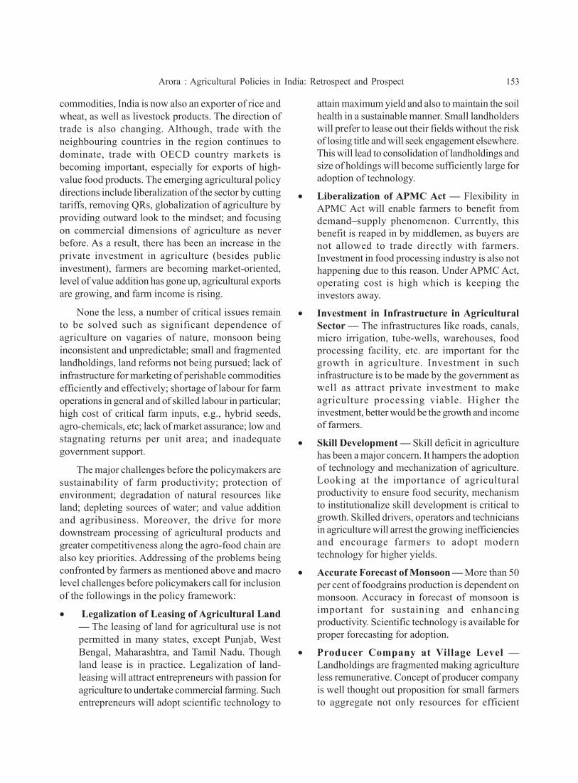
Arora : Agricultural Policies in India: Retrospect and Prospect 153
commodities, India is now also an exporter of rice andwheat, as well as livestock products. The direction oftrade is also changing. Although, trade with theneighbouring countries in the region continues todominate, trade with OECD country markets isbecoming important, especially for exports of high-value food products. The emerging agricultural policydirections include liberalization of the sector by cuttingtariffs, removing QRs, globalization of agriculture byproviding outward look to the mindset; and focusingon commercial dimensions of agriculture as neverbefore. As a result, there has been an increase in theprivate investment in agriculture (besides publicinvestment), farmers are becoming market-oriented,level of value addition has gone up, agricultural exportsare growing, and farm income is rising.
None the less, a number of critical issues remainto be solved such as significant dependence ofagriculture on vagaries of nature, monsoon beinginconsistent and unpredictable; small and fragmentedlandholdings, land reforms not being pursued; lack ofinfrastructure for marketing of perishable commoditiesefficiently and effectively; shortage of labour for farmoperations in general and of skilled labour in particular;high cost of critical farm inputs, e.g., hybrid seeds,agro-chemicals, etc; lack of market assurance; low andstagnating returns per unit area; and inadequategovernment support.
The major challenges before the policymakers aresustainability of farm productivity; protection ofenvironment; degradation of natural resources likeland; depleting sources of water; and value additionand agribusiness. Moreover, the drive for moredownstream processing of agricultural products andgreater competitiveness along the agro-food chain arealso key priorities. Addressing of the problems beingconfronted by farmers as mentioned above and macrolevel challenges before policymakers call for inclusionof the followings in the policy framework:
• Legalization of Leasing of Agricultural Land— The leasing of land for agricultural use is notpermitted in many states, except Punjab, WestBengal, Maharashtra, and Tamil Nadu. Thoughland lease is in practice. Legalization of land-leasing will attract entrepreneurs with passion foragriculture to undertake commercial farming. Suchentrepreneurs will adopt scientific technology to
attain maximum yield and also to maintain the soilhealth in a sustainable manner. Small landholderswill prefer to lease out their fields without the riskof losing title and will seek engagement elsewhere.This will lead to consolidation of landholdings andsize of holdings will become sufficiently large foradoption of technology.
• Liberalization of APMC Act — Flexibility inAPMC Act will enable farmers to benefit fromdemand–supply phenomenon. Currently, thisbenefit is reaped in by middlemen, as buyers arenot allowed to trade directly with farmers.Investment in food processing industry is also nothappening due to this reason. Under APMC Act,operating cost is high which is keeping theinvestors away.
• Investment in Infrastructure in AgriculturalSector — The infrastructures like roads, canals,micro irrigation, tube-wells, warehouses, foodprocessing facility, etc. are important for thegrowth in agriculture. Investment in suchinfrastructure is to be made by the government aswell as attract private investment to makeagriculture processing viable. Higher theinvestment, better would be the growth and incomeof farmers.
• Skill Development — Skill deficit in agriculturehas been a major concern. It hampers the adoptionof technology and mechanization of agriculture.Looking at the importance of agriculturalproductivity to ensure food security, mechanismto institutionalize skill development is critical togrowth. Skilled drivers, operators and techniciansin agriculture will arrest the growing inefficienciesand encourage farmers to adopt moderntechnology for higher yields.
• Accurate Forecast of Monsoon — More than 50per cent of foodgrains production is dependent onmonsoon. Accuracy in forecast of monsoon isimportant for sustaining and enhancingproductivity. Scientific technology is available forproper forecasting for adoption.
• Producer Company at Village Level —Landholdings are fragmented making agricultureless remunerative. Concept of producer companyis well thought out proposition for small farmersto aggregate not only resources for efficient

154 Agricultural Economics Research Review Vol. 26 (No.2) July-December 2013
utilization but also decision-making process likewhat crop to grow, which varieties to use, whereto buy seed from, when to sow, etc. Producercompany concept facilitates this in mostdemocratic manner for the benefit of all.
• Mechanization of Small Farms — Shortage oflabour is the biggest pain farmers are experiencingpost-MNREGA. Mechanization is the answer.This is not possible unless sufficient skills aredeveloped at the village level. Besides,government needs to provide support, especiallyat the initial stages, for promotion and adoptionof mechanized operations.
• Regulatory Authority in Agriculture — Landbeing a precious resource of the country with highpopulation, cannot be allowed to be under-used.Regulatory authority in agriculture must developprocesses and systems to gauge and monitoroptimum utilization of land for foodgrainproduction.
• Government Support Commensurates withFarmers in Agriculturally-advanced Countries— In the global economy, farmers from not sorich countries suffer due to uneven support of thegovernment. In a free market, support needs to beequitable to provide level playing fields to all andremove any natural or manmade advantages in thelarger interests of the farmers with lower income.
• Food Processing — Food habits in urban Indiaare fast changing, creating the need to promotefood processing. A proper mechanism is to betabled in a phased manner to encourage changesin food habits in the urban areas. Cold chains,warehouses, processing facilities, etc. willautomatically flourish as a result of growingdemand for processed foods in the urban areas.This will also establish strong linkages betweenrural and urban economy for mutual benefits.
• Leverage Potential of Hills — Hills are boon forany nation. They provide diversity in climate,flora–fauna and opportunity to grow what cannotbe grown in the plains. The potential of hills hasto be assessed properly and investments oninfrastructure have to be made to exploit theopportunity for the benefit of all.
BibliographyAcharya, S.S. (1985) Regulation of agricultural produce
markets, some observations on the impact, DevelopmentPolicy and Administrative Review, 11(2): July-December.
Acharya, S.S. (1988) Agricultural Production, Marketingand Price Policy in India, Mittal Publishers, New Delhi,pp. 317; 320-27.
Bhalla, G.S. and Singh, G. (1997) Recent developments inIndian agriculture: A state level analysis, Economic andPolitical Weekly, 32(March): A2.18.
Bhattacharya, B. and Pal, Parthapratim (2002) Agriculturaltrade policy during the tenth five year plan, AgriculturalSituation in India, LIX(5): 255-258.
CMIE (Centre for Monitoring Indian Economy), PublicFinance (various Issues).
Chadha, G.K. (2002) Indian agriculture in the newmillennium: Human response to technology challenges,Presidential address delivered at 62nd AnnualConference of Indian Society of AgriculturalEconomics, IARI, New Delhi
Chadha, G.K. and Sahu, P.P. (2002) Post reforms setback inrural employment: Issues that need further scrutiny,Economic and Political Weekly, 37(21), May 25.
Chand, Ramesh (2002) Trade Liberalisation, WTO andIndian Agriculture: Experience and Prospects, MittalPublications, New Delhi.
Chand, Ramesh (2003a) Government Intervention inFoodgrain Markets in the Changing Context, PolicyPaper 19, National Centre for Agricultural Economicsand Policy Research, New Delhi.
Chand, Ramesh (2003b) Minimum support price inagriculture: Changing requirements, Economic andPolitical Weekly, 38(29): 3027-3028.
Chand, Ramesh, Kumar, P. and Sinha, Sapna (2003) Impactof Agricultural Trade and Related Reforms on DomesticFood Security in India, Report of the study done forFAO Rome, Institute of Economic Growth, Delhi,November.
Dholkia, Bakul H. (1997) Impact of economic liberalisationon the growth of Indian agriculture, In: AgriculturalDevelopment Paradigm for the Ninth Plan Under NewEconomic Environment, Ed: Bhupat M. Desai, Oxfordand IBH Publishing Co. Pvt. Ltd, New Delhi.
Fan, S., Hazell, P. and Thorat, S. (1999) Linkages betweenGovernment Spending, Growth, and Poverty in RuralIndia, Research Report 110, IFPRI, Washington, DC.

Arora : Agricultural Policies in India: Retrospect and Prospect 155
Fan, S., Hazell, P. and Thorat, S. (2000) Governmentspending, growth and poverty in rural India, AmericanJournal of Agricultural Economics, 82(4): 1038.51.
Fan, S., Hazell, P. and Thorat, S. (2001), Returns to publicinvestments in the less-favored areas of India and China,American Journal of Agricultural Economics, 83(5):1217.22.
GoI (Government of India) (2012) Agricultural Statisticsat a Glance, Ministry of Agriculture and Cooperation,New Delhi.
GoI (Government of India) (2012-13) Economic Survey,Economic Division, Ministry of Finance & CompanyAffairs, New Delhi.
Haque, T. (2003) Land reforms and agriculturaldevelopment: Retrospect and prospect, In: InstitutionalChange in Indian Agriculture, Eds: Suresh Pal,Mruthyunjaya, P. K. Joshi and Raka Saxena, NationalCentre for Agricultural Economics and Policy Research,New Delhi.
Jha, S. and Umali-Deininger, D. (2003) Public Expenditureson Food and Nutrition Security Programs in India: AreThey Meeting the Challenge, Rural Development SectorUnit, Working Paper, World Bank, Washington, DC.
Kahlon, A.S. and George, M.V. (1986) AgriculturalMarketing and Price Policies, Allied Publishers, NewDelhi.
Krishnaswamy, K.S. (1994) Agriculture development underthe new economic regime, Economic and PoliticalWeekly, 29(26): A-65 . A-71.
Marothia, D.K. (2003) Institutions for common poolresources, In: Institutional Change in IndianAgriculture, Eds: Suresh Pal, Mruthyunjaya, P. K. Joshiand Raka Saxena, National Centre for AgriculturalEconomics and Policy Research, New Delhi.
Mehta, Rajesh and George, J. (2003) Implementation issuesin SPS: A developing country perspective fordevelopment agenda on the mmeandering pathwaysfrom Doha to Cancun, RIS Discussion Paper 58,Research and Information System for Non Aligned andOther Developing Countries, New Delhi.
Ministry of Agriculture (2000) National Agricultural Policy,Department of Agriculture and Cooperation, NewDelhi.
Nayyar, Deepak and Sen, Abhijit (1994) International tradeand agricultural sector in India, In: EconomicLiberalisation and Indian Agriculture, Ed: G.S. Bhalla,Institute for Studies in Industrial Development, NewDelhi.
Pal, Suresh and Saxena, Raka (2003) Agricultural R&Dreforms in India: Policy and institutional imperatives,In: Institutional Change in Indian Agriculture, Eds:Suresh Pal, Mruthyunjaya, P. K. Joshi and Raka Saxena,National Centre for Agricultural Economics and PolicyResearch, New Delhi.
Pal, Suresh, Mruthyunjaya, Joshi, P.K. and Saxena, Raka(2003) Institutional change in Indian agriculture: anoverview, In: Institutional Change in IndianAgriculture, Eds: Suresh Pal, Mruthyunjaya, P. K. Joshiand Raka Saxena, National Centre for AgriculturalEconomics and Policy Research, New Delhi.
Rao, C.H. Hanumantha and Gulati, Ashok (1994) Indianagriculture: Emerging perspective and policy issues,Economic and Political Weekly, 29(53): A-158 . A-170.
Rao, V.M. (1994) Agriculture and liberalisation: Someimplications for development policies, Economic andPolitical Weekly, 29(16/17): 999-1004.
Reddy, V. Ratna and Badri Narayan, K. (1992) Tradeexperience of Indian agriculture: Behaviour of netexport supply function for dominant commodities,Indian Journal of Agricultural Economics, 47(1):January- March.
Satyasai, K.J.S. (2003) Micro-finance in India: Progress andperspectives, In: Institutional Change in IndianAgriculture, Eds: Suresh Pal, Mruthyunjaya, P. K. Joshiand Raka Saxena, National Centre for AgriculturalEconomics and Policy Research, New Delhi.
Singh, R.B., Kumar, P. and Woodhead, T. (2002)Smallholder Farmers in India: Food Security andAgricultural Policy (FAO Study), RAP Publication:2002/03, Food and Agriculture Organisation of theUnited Nations, Regional Office for Asia and thePacific, Bangkok, Thailand, 54 p.
Schultz, T.W. (1964) Transforming Traditional Agriculture,Yale University Press, New Haven, CT.
Vaidyanathan, A. (1996) Agricultural development:Imperatives of institutional reforms, Economic andPolitical Weekly, 31(35/37): 2451-2458.
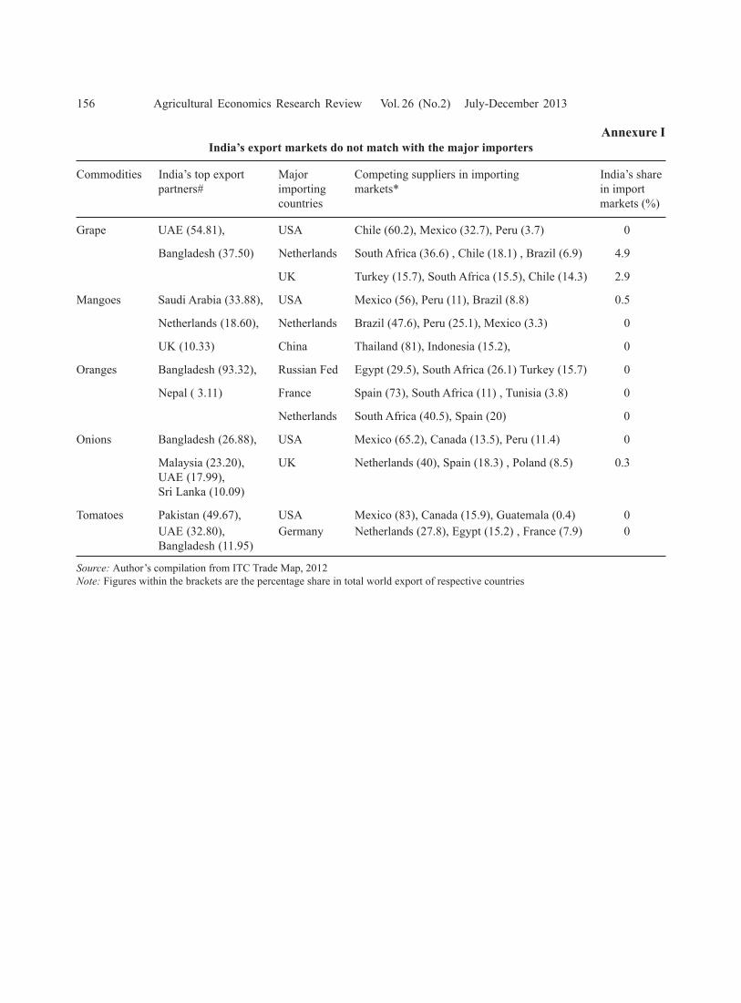
156 Agricultural Economics Research Review Vol. 26 (No.2) July-December 2013
Annexure IIndia’s export markets do not match with the major importers
Commodities India’s top export Major Competing suppliers in importing India’s sharepartners# importing markets* in import
countries markets (%)
Grape UAE (54.81), USA Chile (60.2), Mexico (32.7), Peru (3.7) 0
Bangladesh (37.50) Netherlands South Africa (36.6) , Chile (18.1) , Brazil (6.9) 4.9
UK Turkey (15.7), South Africa (15.5), Chile (14.3) 2.9
Mangoes Saudi Arabia (33.88), USA Mexico (56), Peru (11), Brazil (8.8) 0.5
Netherlands (18.60), Netherlands Brazil (47.6), Peru (25.1), Mexico (3.3) 0
UK (10.33) China Thailand (81), Indonesia (15.2), 0
Oranges Bangladesh (93.32), Russian Fed Egypt (29.5), South Africa (26.1) Turkey (15.7) 0
Nepal ( 3.11) France Spain (73), South Africa (11) , Tunisia (3.8) 0
Netherlands South Africa (40.5), Spain (20) 0
Onions Bangladesh (26.88), USA Mexico (65.2), Canada (13.5), Peru (11.4) 0
Malaysia (23.20), UK Netherlands (40), Spain (18.3) , Poland (8.5) 0.3UAE (17.99),Sri Lanka (10.09)
Tomatoes Pakistan (49.67), USA Mexico (83), Canada (15.9), Guatemala (0.4) 0UAE (32.80), Germany Netherlands (27.8), Egypt (15.2) , France (7.9) 0Bangladesh (11.95)
Source: Author’s compilation from ITC Trade Map, 2012Note: Figures within the brackets are the percentage share in total world export of respective countries

Arora : Agricultural Policies in India: Retrospect and Prospect 157
Annexure IINon-tariff barriers on India’s agricultural exports to the EU, USA and Japan
Product Non-tariff barriers Country
Spices No uniform standard and common regulation in EU. No fixed permitted level Spain, Italy(chillies) of aflatoxin or pesticide residue. Adversely affecting spices exports from India. and Germany
Meat India free from rinderpest since 1995 still export to EU not permitted EU
Milk Exports to EU not permitted as Indian cows are not mechanically milked EU
Fishery EU put a ban in 1997. Allows only the form at its approved plants in India. EUproduct standards for fishery products are very stringent, cumbersome, and costly EU
Peanut Aflatoxin standards of EU are more stringent than international standards on EUIndia’s export. Prescribed testing method known as Dutch code and otherrequired methods are very rigorous and very costly. Permissible limits aredifferent in different countries and keep changing. Some tests are required onlyfor India and Egypt and not for exports from USA and Argentina.
Mango and Requirement of costly vapour heat treatment for export of fresh mango, US, Japan,mango pulp labelling, pesticide residues. and Jordan
Rice Pesticide residues consignment of basmati and rice rejected in US on ground of EU, Japan, USAbeing filthy and containing foreign matter. US regulation require manual sortingof rice and fumigants and weevils have to be blown out. Delay in clearingconsignments, repeated tests.
Tea Pesticide residue. Complaint of high residue level of Ethicon in Darjeeling tea EU and Germany
Fish Anti-dumping duty imposed by US on Indian shrimp in 2005 USA
Tobacco Internationally permissible level of DDT residue is 6 ppm while Japan and USA Japan, USAhad set their DDT levels at much lower level; Japan insists on 0.4 ppm of DDTlevel Indian tobacco has DDT level of 1-2 ppm which is well below theinternational standard but Japan does not allow tobacco import from India.
Egg powder Consignment first time subjected to additional criteria of MRPL (minimum EUrequired performance limit) in May 2003 despite valid equivalence issued byEU. No action on applications for equivalence for 7-8 years.
Sources: Adapted from Jha (2003 ); Mehta and George (2003); RIS (2003)


Agricultural Economics Research ReviewVol. 26 (No.2) July-December 2013 pp 159-172
The State of Agricultural Extension Reforms in India:Strategic Priorities and Policy Options§
Suresh C. Babua* , P.K. Joshib, Claire J. Glendenningc, Kwadwo Asenso-Okyerec
and Rasheed Sulaiman V.d
aInternational Food Policy Research Institute, Washington DC, USAbInternational Food Policy Research Institute, New Delhi-110 012, India
cFormerly at International Food Policy Research Institute, Addis Ababa, EthopiadCentre for Research on Innovation and Science Policy, Hyderabad, Andhra Pradesh, India
Abstract
Agricultural extension in India has undergone several changes since independence. Still, a large numberof smallholder farmers and other vulnerable groups remain unreached by the public extension system. Anumber of organizational performance issues hinder the effectiveness and efficiency of public extensionsystem. These include inadequate staff numbers, low partnerships, and continued top-down linear focusto extension. This paper has presented a critical review of the current state of agricultural extensionreforms in India and based on the field case studies in four states —Bihar, Himachal Pradesh, Maharashtra,and Tamil Nadu —has identified policy priorities and strategic options for further refining the on-goingreform process and effective implementation of the public agricultural extension system.
Key words: Agricultural extension, strategic priorities, policy options, extension reforms
JEL Classification: Q16, Q18
IntroductionThe Indian agriculture is at the crossroads today.
Its strength to alleviate poverty and hunger is well-recognized, yet, the agricultural growth rate in the past20 years has been visibly less impressive and the
productivity in the agricultural sector continues to below compared to the international standards. Whileinvestments in research and extension have increasedin recent years, their impact on smallholder farmers’livelihoods remains debatable. Even when theseinvestments may address relevant problems of thefarmers, the benefits of improved technologies will notfully accrue to the farmers. The yield gap betweenresearch stations and farmers’ field remains high. Fortranslating research results into tangible gains at farm-level, well-functioning agricultural extension andadvisory services are required.
The Indian public agricultural extension system isone of the largest knowledge and informationdissemination institutions in the world. The systemplayed a critical role during the Green Revolutionperiod, but in recent years, it has undergone a high
*Author for correspondenceEmail: [email protected]
§ This is a substantially expanded version of the paperpresented at the workshop on ‘Policy Options and InvestmentPriorities for Accelerating Agricultural Productivity andDevelopment in India’, organized by the Indira GandhiInstitute of Development Research, Mumbai and the Institutefor Human Development with the support from the PlanningCommission, Government of India, Food and AgricultureOrganization (FAO) and The World Bank, during 10-11November, 2011 in New Delhi. We are grateful to FAO- NewDelhi for funding this study and for the discussions andcomments during the above workshop. Usual disclaimersapply.

160 Agricultural Economics Research Review Vol. 26 (No.2) July-December 2013
level of scrutiny (Sontakki et al., 2010; Pal, 2008; Joshiet al., 2005). Several efforts have been made in thepublic sector over the past one decade to initiate variousreform measures and operational models to improvethe organizational performance of this system. Yet, thechallenge of enhancing relevance, efficiency, andeffectiveness of the public sector agricultural extensionsystem in meeting its organizational goals andobjectives remains unresolved (WGAE, 2007; Raabe,2008; Glendenning et al., 2010; Desai et al., 2011).
Undoubtedly, without a well-functioning nationalagricultural research system (NARS) capable toproduce relevant technologies and knowledge base, anyamount of reforms in the agricultural extension systemwill be unsuccessful (Binswanger-Mkhizi and Zhong,2012). The reforming of NARS in India has been thesubject of extensive analysis and the focus of severalhigh-powered committees (NAAS, 2005; NFC, 2006;Pal, 2008; ICAR, 2011). India is endowed with a strongNARS, comprising the Indian Council of AgriculturalResearch (ICAR) and State Agricultural Universities(SAUs). The ICAR is the apex body for agriculturalresearch and education in the country. The contributionsof agricultural research have been commendable to theglobal agri-food systems, especially during the GreenRevolution period in the mid-1960s and early-1970s.A perfect symphony of research, technology, and inputdelivery, and agricultural policies was responsible forthe impressive performance of Indian agriculture inthe 1970s and the 1980s. The production of rice andwheat witnessed a spectacular increase, andtransformed Indian agriculture from deficit to self-sufficiency in food grains (Joshi et al., 2005). Althoughthe NARS has been responding to the challenges facedby Indian agriculture, it is often criticized for notattending to the demands for improved technologiesand also for the poor linkages between research andextension systems (Desai et al., 2011).
This paper examines the current state ofagricultural extension reforms and their linkages to theagricultural research system reforms in India, andidentifies the policy options and strategic priorities formaking it relevant, responsive and efficient. It exploreshow the NARS responded with its own set of reformsthat were sought to increase its relevance and itslinkages to the extension systems reforms. It alsoprovides an assessment of the organizationalperformance of the major public sector policy reforms
in the agricultural extension — the AgriculturalTechnology Management Agency (ATMA) model —using the case studies of seven districts in four Indianstates (Bihar, Himachal Pradesh, Maharashtra andTamil Nadu), located in different agro-ecological zonesof the country.
The paper is organized in seven sections. After abrief background in section one, the following sectionprovides the evolution of agricultural extension systemin the country. In section three, a snap-shot on emergingchallenges and issues for agricultural extension andadvisory services is given. Farmers’ access and sourcesof extension are discussed in section four, using NSSOdata and also several case studies conducted in recentyears. Section five examines the performance ofAgricultural Technology Management Agency withrespect to its relevance and reach to the farmers. It isfollowed by the section that prescribes policies andstrategies for reforming agricultural extension systemin the country. Finally, in the last section, we concludethe conditions for successful extension reforms in thecountry.
Evolution of the Extension System in IndianAgriculture
The evolution of agricultural extension system inIndia has a long history. Its contribution to productivityenhancement during the Green Revolution era has beenwell documented. During this period, the publicextension system played the key role in conductingfield demonstrations of high-yielding varieties andimproving the input delivery that ensured timelyavailability of quality seeds, fertilizers and agriculturalchemicals at affordable prices. Along with extensionservices, the price policy and procurement supportthrough public agencies provided additionalencouragement to the farmers for adoption of high-yielding varieties in the 1960s and 1970s. By the endof 1970s, the Green Revolution type of extensionsystem had largely achieved its major goal of increasingthe area under high-yielding varieties (Ameur, 1994).
In the late-1970s, the agricultural extension systembecame mostly involved in the distribution ofagricultural inputs through the state agricultural depotsand handling of the subsidies that were providedthrough various agricultural development programs.The public sector extension system as a whole seemed

Babu et al. : The State of Agricultural Extension Reforms in India 161
to have become a monolithic organization withoutspecific goals to achieve. Sustaining such a large systemwithout added benefits to agricultural productivitybecame a big challenge for agriculture ministries atboth the central and state levels. Therefore, reformingof the system towards goal orientation and betteroperational efficiency was sought. A Training and Visit(T&V) system was introduced in extension serviceson a pilot scale in Rajasthan in 1974 with World Bankfunding support and was scaled up to several otherstates in 1977 (Ameur, 1994). While impressive resultswere documented by the studies that evaluated the T&Vsystem, the issues related to sustainability of funding,high requirement of staffing, and the quality of staffbecame the key concerns (Federet al., 1987; Andersonand Feder, 2004). The state governments could not meetthe high level of recurrent costs of the system andstopped recruitment of new staff after the World Bankfunding ended in the early-1990s. Over the next tenyears, due to the low level of staff and low resourcesto cover their costs, no serious efforts were made tohold the extension officials accountable. No specificgoals were set and the agricultural extension systemas a whole had become moribund, although the T&Vsystem continued as a method of public extension(Anderson et al., 2006). Thus, began a period of lowcommitment from the policymakers at the state level.This was reinforced by the ineffectiveness of theextension system as a whole in contributing to farmers’needs. As a result, the T&V system, or whateverremained of it, was seen as an unrealistic model bymany state governments, though some elements of themodel still continue to be implemented in several states.
About a decade ago, in order to introduce reformsin the public sector agricultural extension system andincrease its relevance, accessibility, and efficiency ofknowledge sharing among various actors, players, andstakeholders, the Agricultural Technology ManagementAgency (ATMA) was introduced as a pilot (1998-2003)in 28 districts (DAC, 2005). Following a positivefeedback from the pilot implementation (IIM, 2004),the ATMA model was scaled up across 251 ruraldistricts in 2005 and throughout the country in 2007(Reddy and Swanson, 2006). In June 2010, revisedguidelines for ATMA were issued in order toincorporate the lessons learnt from the implementationthus far (DAC, 2010). However, several operationaland organizational challenges continue to confront the
ATMA as a system of extension. The ATMA facessevere capacity and institutional constraints. Yet,ATMA is seen as the key intervention for reformingthe extension system in India. There is increased callfor evaluating the impact of ATMA model on the farmlevel benefits. However, an understanding of thevariance between the intended guidelines and the actualimplementation of the program is still lacking. Further,the organizational and capacity challenges in itsimplementation have not been fully recognized(Anderson, 2007). Such information is the first steptowards the analysis of the impact of the program. Inwhat follows we take a critical look at theorganizational performance issues faced in theimplementation of ATMA to provide program andpolicy feedback for further refining the reform process.But, first we examine the global patterns in extensionreforms, followed by the existing use of extension bythe farmers in India.
Issues for Extension and Advisory ServicesIndia is not alone in the world in reforming its
extension and research systems. There are manycountries where extension and advisory servicesreforms are occurring globally (Swanson and Rajalahti,2010; World Bank, 2012). A common pattern in mostdeveloping countries is to decentralize the extensionsystems since agro-ecological conditions and accessto markets vary within most countries. Makingextension decentralized and demand-driven gives thefarmers a better say in setting the agenda anddemanding extension and research priorities. Theextension reforms strive to reach those groups —smallholders, resource-poor, and women farmers —which often remain unreached by the existing extensionsystems, and instead often tend to address the needs ofprogressive and commercially-viable farmers. Thereform measures also focus on sustainability. Withoutadequate public funding, agricultural extension systemsin many developing countries will not be sustainablein the long-run. Donor funds are not highly reliableand are targeted mostly to pilot projects. When thedonor funds dry up or the pilot projects end, the farmersno longer have access to the extension services (Birnerand Anderson, 2007). The public sector has a role toplay in developing a sustainable system of extensionservices delivery. Recognizing that a top-downapproach does not always address the needs of farmers,

162 Agricultural Economics Research Review Vol. 26 (No.2) July-December 2013
extension reforms also focus on making extension andadvisory services farmer-led and demand-driven.However, in any extension reform, poorly developedand inadequate monitoring systems, coupled with lowhuman and institutional capacities, remain a majorconstraint to scaling-up successful pilot programs.Another reform option is the increased use of moderninformation and communication technologies (ICTs),but this calls for a higher level of investment in orderto make them accessible by the smallholder farmers(Aker, 2011). Given the broad lessons emerging fromglobal experiences and the immediate need forunderstanding the challenges and constraints incontinuing the reforms in agricultural extension systemin India, we next review the farmers’ access toagricultural extension and advisory services and thevarious sources from which farmers access theseservices in the context of extension system reforms.
Farmers’ Access and Sources of ExtensionServices
The only nation-wide survey of farmers’ access toextension is the 2003 National Sample SurveyOrganization (NSSO) 59th round, 33rd schedule on‘Situation Assessment Survey of Farmers’. Sixty percent of the farmer-households in India did not accessany information on modern technologies that year. Thatsuch a large proportion of the farming population doesnot use any extension service indicates the poororganizational performance of the public extension in2003. It was aptly identified in the 10th and 11th five-year plans, which recognized that the public extensionsystem needed ‘revamping’ and ‘revitalizing’.
While a more recent nation-wide survey is notavailable, a number of IFPRI studies have shown apicture different from the NSSO 2003 survey. In TamilNadu, a 576 farmer-households survey in two districtshas shown that only 1 per cent of the respondents hadnot accessed any information to support their farmenterprise in 2010. By comparison in 2003, the NSSOsurvey data show that 50 per cent of the farmers inTamil Nadu did not access extension for information.From a survey of farmer-households, Birner andAnderson (2007) have reported that of the 966 farmer-households surveyed, 22 per cent had at least onecontact with a government extension worker duringthe past one year, which was greater than the averageof 11.5 per cent reported for Karnataka in the NSSO
2003 survey (NSSO, 2005). A survey of 810households each in Uttar Pradesh, Madhya Pradesh andAndhra Pradesh revealed a different extent ofextension-use in these states in 2009; it was 18 percent in Uttar Pradesh (Reardon et al., 2011a), 80 percent in Madhya Pradesh (Reardon et al., 2011b) and95 per cent in Andhra Pradesh (Chandrasekhar et al.,2011). While the recent small-scale surveys have shownthat extension access might have improved since thetime of the NSSO 2003, a nation-wide survey is neededto show the difference in extension-use since theimplementation of major reforms in public sectoragricultural extension through programs like the‘Support to State Extension Programs for ExtensionReform’ (SSEPER) and the Agricultural TechnologyManagement Agency (ATMA).
Progressive farmers and family members, as wellas mass media and the private sector constitute a largepast of farmers’ sources of information. Another issueis that the quality and reliability of public extensionsystem is still a constraint (Babu et al., 2012). Onsources of extension services, the NSSO survey resultshave shown that nearly one-third of the farmers whohad accessed information, obtained it from progressivefarmers and input dealers. Broadcast media, includingradio, television and newspapers, was also largely usedto obtain information (by about 29.3% farmers). Thepublic sector extension system was a source ofinformation for about 10 per cent of the farmers. Theprivate and NGO extension services were accessed byonly 0.6 per cent of the farmers. Farmers tried andadopted the information that they received fromprogressive farmers and input dealers more than fromother sources. The service delivery by public-sectorextension workers was lowest for small farmers (4.8%versus 12.4% for large farmers), which suggests thatthe system may be biased against small farmers(Adhiguru et al., 2009).
In a recent survey of farmers in Tamil Nadu in2010, the input dealer was reported to be the mainsource of information (68.6%), followed by the statedepartment of agriculture extension staff (51.2%), TV(43.6%), family members or relatives (39.9%),progressive farmers (36.2%), Primary AgriculturalCooperative Banks (35.7%) and newspapers (30.6%).Farm magazines were accessed by 9.2 per cent of thefarmers. Only a small percentage of farmers used radio(5.4%) and farmer group associations (4.7%) to access

Babu et al. : The State of Agricultural Extension Reforms in India 163
information (Babu et al., 2012). The main reasons forthe choice of information source were proximity(33.7%), assured quality (21.1%), sole option (20.6%),and timely availability (13.7%).
In Uttar Pradesh, Reardon et al. (2011a) havereported that 7 per cent of the sample farmers availedthe services of state extension staff, while other public-sector extension sources (KVKs, All-India Radio,university extension, and plant protection units) werecollectively a source of information for 18 per cent ofthe farmers. Madhya Pradesh has presented a morepositive picture of public sector extension-use, with37 per cent of the farmers accessing state extensionstaff (Reardon et al., 2011b). Other major sources ofextension services for farmers in Madhya Pradesh wereAll-India Radio and TV (21%), and KVKs (12%). Theprivate-sector sources accounted for 25 per cent.
The studies reported above suggest that theorganizational performance of extension system couldbe influenced by local conditions. Therefore, reformsin the extension system would need to allow flexibilityin the service delivery to adapt to different situations.Consideration of state variabilities is important indeveloping extension strategies, particularly at thenational level where much of the public sectorextension policy is formulated. A greater flexibility atthe state level to implement effective extensionprograms is needed.
The provision and delivery of agriculturalextension and advisory services to small and marginalfarmers remain the important elements of extensionreforms in the developing countries. The challenge forsmallholder farmers in India is typical (Birner andAndersen, 2007; Chandrasekhar Rao et al., 2011;Reardon et al., 2011a; 2011b). These farmers tend tohave minimum access to information. Reachingfarmers who search for information the least, would,therefore, require different content, approach anddelivery mechanisms, as they have differentinformation needs and rely mostly on interpersonalsources. Targeting smallholder farmers, who have lowagricultural income, is important as they search lessfor information. These farmers mostly lack motivationand interest in agriculture, so improving the timelydelivery and reliability of information will be importantto encourage them to improve their information searchstrategies. The studies have revealed that membershipof farmer based organizations (FBO) is associated with
high information search behaviours. Being a significantfactor in determining information search behaviours,membership in a FBO, self-help group (SHG) orcooperative could be an approach extension servicescould target to improve access to extension of low andmoderate information searchers. A group-basedapproach could also improve the delivery of demand-driven extension services. This is the main aim ofdistrict level public extension institution, the ATMA,though several implementation issues are hindering itseffectiveness. Further, the public sector is only one ofthe many sources farmers use to access extension andadvisory services.
Pluralistic Extension and Advisory Services andtheir Performance
The public sector agricultural extension system inIndia has gone through a number of changes sinceindependence (Glendenning et al., 2010; Raabe, 2008;Sulaiman and Holt, 2002). Still, several organizationalperformance issues hinder the effectiveness andefficiency of public agricultural extension system.These include inadequate staff numbers, lowpartnerships, and continued top-down linear focus toextension. Innovations from the private sector and civilsociety organizations show that providing an integratedservice to farmers, which incorporates local needs,could be more relevant. But, it is clear that the privateand civil society sectors will not fulfil the entire roleof extension and advisory service in India. The privatesector should work in areas where business issustainable and should interact with farmers on anindividual basis. The civil society tends to be project-based and is not widespread. On examining where thecapacity lies in each sector, partnerships emerge as animportant need; non-governmental organizations(NGOs) and civil society organizations (CSOs) havethe capacity to build social capital, but they tend towork on a small scale; the technical expertise lies inthe national agricultural research system (ICAR andstate agricultural universities), but it is also not able toreach a reasonable scale with limited staff in eachdistrict; the private sector can improve market linkages;and the state department of agriculture has the reachacross each district of India, but staff are overburdenedwith other duties.
During the past ten years, the central governmenthas recognised the need to converge and integrate

164 Agricultural Economics Research Review Vol. 26 (No.2) July-December 2013
extension activities at the district level and hasimplemented a major reform in extension. It aims toachieve this through the institution of AgricultureTechnology Management Agency (ATMA). While thisis viewed as a huge innovation in agricultural extensionsystem r, it is also not without implementation andorganizational challenges.
Organizational Performance Assessment ofAgricultural Technology Management Agency
The Agricultural Technology Management Agency(ATMA) is the flagship program for agriculturalextension reforms in India. It was implemented as apilot in 28 districts from 1998 to 2004 as part of theWorld Bank-funded Innovations in TechnologyDissemination (ITD) component of the NationalAgriculture Technology Project (NATP) (Reddy andSwanson, 2006; Singh and Swanson, 2006; Swanson,2008). The constraints of the Training and Visit (T&V)and post-T&V extension were considered to beaddressed in the ATMA pilot.
Over the past one decade, the implementation ofextension reforms in the form of ATMA has gonethrough three phases; the NATP pilot 1998-2004 ATMA(phase I), the 2005-2010 Government of India (GoI)ATMA (phase II), and the post-2010 GoI ATMA (phaseIII). On the basis of the ATMA pilot, in 2005-06 theGovernment of India initiated the Support to StateExtension Programs for Extension Reforms (SSEPER)project, which was operationalized through ATMA,across 262 districts in all states —about one-third ofall districts in India. In 2007, the XIth Five-Year Planexpanded ATMA to all the districts of India, but it wasnot supported with the provision of additional fundingand staff. The XIth Five-Year Plan working group onagricultural extension (WGAE, 2007) identified theorganizational performance challenges of the program,including (i) lack of qualified personnel at all levels,(ii) absence of a formal mechanism to support extensiondelivery below the block level, (iii) inadequateinfrastructure support at the state agriculturalmanagement and extension training institutes(SAMETIs), and (iv) lack of convergence with othercentral and state projects. It was not until 2010 that theplan for increased funding to ATMA was approved,resulting in revised guidelines for the ATMA (DAC,2010).
ATMA is a registered society at the district level.The district extension activities are based on a strategicresearch and extension plan (SREP) prepared using theparticipatory rural appraisal (PRA) technique for eachdistrict. The ATMA governing board (AGB), chairedby the district magistrate, reviews and approves theSREP for the district and also the annual block actionplans (BAP). Other members of the board include theheads of line departments and research organizationsas well as stakeholder representatives, includingfarmers and private sector representatives. The ATMAproject director chairs the ATMA managementcommittee (AMC). The AMC is responsible forcoordinating the extension activities in the district. TheAMC includes the heads of all line departments andresearch organizations in the district.
At the block level, the farm information andadvisory centre (FIAC) is the physical platform wherethe block technology team (BTT) and farmer advisorycommittee (FAC) meet to prepare the block action plan(BAP) and implement extension activities. The BTTincludes technical officers from various linedepartments at the block level and consults with theFAC, which includes the heads or representatives offarmer interest groups (FIGs) and self-help groups(SHGs). When FAC approves the BAP, it is reviewedby the AMC and approved for funding by the AGB.The FAC meets monthly to discuss the implementationof the annual BAP. The decision-making process isdecentralized to the block level, with activeparticipation of farmer representatives in thedevelopment and approval of the BAP.
At the state-level, an interdepartmental workinggroup (IDWG) formulates a state extension work plan(SEWP) to consolidate the district SREPs. The SREPand SEWP are the instruments that promoteconvergence of extension activities between linedepartments and research institutions at the district andstate levels, respectively. In each state, a stateagricultural management and extension traininginstitute (SAMETI) has been established. This instituteprovides training and undertakes human resourcedevelopment on the concepts and processes of ATMAto the junior and middle-level extension functionaries.The current performance of ATMA at all of these levelsvaries from state to state.

Babu et al. : The State of Agricultural Extension Reforms in India 165
In 2010, the Department for Agriculture andCooperation (DAC) released new guidelines for ATMA(phase III), which included a revised structure. Theblock to village extension link was formallyinstitutionalized through the concept of a “farmerfriend” (FF) for every two villages. A farmer friend isa progressive farmer who has the minimumqualification of a pass in matriculation or intermediateexamination and is directly engaged by the blocktechnology manager. Some additional personnelexclusive to the ATMA project have been assigned;these include a state coordinator; faculty and supportingstaff for the SAMETI at the state level; a projectdirector, project deputy directors, and supporting staffat the district level (five employees per district); oneblock technology manager and two subject matterspecialists (SMSs) at the block level. Additionalactivities have been added to the “ATMA cafeteria”(the list of extension-related activities to choose fromfor funding), including farm schools. Farmer advisorycommittees (FACs) at the state, district, and block levelsnow provide advice to the administrative bodies at eachlevel, which were previously defined only at the districtlevel (DAC, 2010).
The block-level structure remains similar to theprevious structure but with higher emphasis onincorporating the ICAR institutes, such as the KrishiVigyan Kendras (Farm Science Centres) (KVKs) andZonal Research Stations (ZRS). It is expected that theKVK scientists will provide technical advice to theBTT and will be involved in preparation of the BAPs.The SREP also aims to involve the Panchayati Rajinstitutions, the lowest tier of local government. At thevillage level, the Agriclinics and Agribusiness projectswill be incorporated into the ATMA structure.
To examine the organizational performance of theATMA, this paper has considered the following factors,in addition to the main processes that ATMA is tryingto reform in the extension system, namely:
• Decentralization — Are the activities of ATMAdetermined from the decisions made at district orblock level? What aspects of organizationalperformance are hindering decentralization ofdecision-making at the district and block levels?
• Linkages in ATMA — Is ATMA integrating theextension-related activities of ICAR institutes,including KVKs, state line departments, NGOs
and the private sector at the district and blocklevels, which have been traditionally working inparallel? What aspects are hindering thisintegration?
• Farmer Participation — Are farmers effectivelyparticipating in decision-making at the block anddistrict levels? What mechanisms are used inATMA to understand the needs/demands offarmers (to make it demand-driven)? What aspectsare hindering farmer participation? What modelof farmer participation is envisaged?
Answers to these questions can help in furtherrefining the design and implementation of ATMA toreach its goals. To understand how ATMA has beenimplemented and how new guidelines may address thechallenges being faced, seven districts in four states— Bihar, Himachal Pradesh, Maharashtra, and TamilNadu— were selected as case studies in 2011-12. Ineach case study, district interviews were conducted withkey informants involved in ATMA at the district andblock levels. This assessment provided a first look athow different states were implementing ATMA, andthe main challenges and constraints in linking differentagencies involved in extension in India, particularlybetween the state department of agriculture and theKVKs, and also empowering farmers to participate andcontribute to block and district level extension plansand programs.
The results from the case studies have highlightedseveral changes brought out by ATMA, although thedegree to which they were achieved in different statesvaried. These included:
• There has been increased recognition of theimportance of extension services by the policy-makers at centre and state levels as evidencedthrough more funding and human resources forextension systems.
• ATMA has expanded the range of extensionactivities (field technology demonstrations, farmertrainings, study tours, farm schools, exhibitions,and farmer-scientist interaction) at the district andblock levels. It has improved the extensionsystem’s ability to respond quickly to the demandsof different stakeholders and thereby has enhancedthe credibility of extension services. It has alsowidened the range of topics dealt with by extensionsystem beyond agriculture.

166 Agricultural Economics Research Review Vol. 26 (No.2) July-December 2013
Figure 1. (a) ATMA in phase I; and (b) ATMA in phase IISource: DAC (2005; 2010)
• ATMA has helped to achieve some convergenceamong different programmes being implementedby the Department of Agriculture (DOA). TheATMA funds are used for trainings and technologydemonstrations to support beneficiaries of severalnational schemes, such as the National FoodSecurity Mission, National Horticulture Mission,etc., which have funds only for distribution ofsubsidized equipments and inputs.
• ATMA has helped to improve workingrelationships of the DOA with other linedepartments (animal husbandry, horticulture,fisheries, sericulture, forestry, and agriculturalengineering), KVKs, research centres of SAUs andICAR, NGOs, and private entrepreneurs involvedin agricultural development. It is partly throughregular meetings at the district and block levelsand partly through additional funding from ATMAthat help some of these departments to implementtheir extension activities.
• ATMA has brought in new concepts, tools, andapproaches to extension planning such as bottom-up planning, farmer involvement in decision-making, participatory rural appraisal, public-private partnerships, commodity interest groups,and beneficiary contributions.
• By implementing a series of activities includingregular staff training through establishment ofSAMETI at the state level, development of theStrategic Research and Extension Plans (SREPS),formation of Commodity Interest Groups (CIGs),and collection of beneficiary contributions, ATMAhas been recognized as a reformed system ofextension at the block and district levels. However,it is yet to establish itself as an autonomousinstitution since it is still implemented as a schemeof the central government and continues to beattached to the DOA at the state and district levels.
• ATMA has created a constituency for its supportat the ground level through the mechanism offarmer advisory committee (FAC) and commodityinterest groups (CIGs) at the local level and tosome extent has expanded public sectorextension’s reach to the rural communities.
• In some states, some of the CIGs are becomingfarmer federations for value addition andmarketing. The registration with ATMA helps theCIGs to better access finance from the commercialbanks to set up processing facilities. ATMA is alsofacilitating the CIGs’ links with other knowledgeand service sources such as marketing agents andequipment manufacturers.
Fund
Flo
w
Wor
k Pl
an
Fund
Flo
w
Wor
k Pl
an
(a) (b)

Babu et al. : The State of Agricultural Extension Reforms in India 167
However, the effectiveness of these initiativesvaries widely from state to state, from district to district,and from block to block, as ATMA’s effectiveness isclosely dependent on the interest and time devoted toit by the officials of DOA and other governmentdepartments, BTT members, BTM and FAC membersas well as their perception of ATMA. Some of thefindings on the factors associated with the performanceof ATMA are discussed below.
• At the district level, the ATMA is recognized as anew demand-driven and multi-agency approachto extension; but at the block levels and withfarmers, this role was not well articulated.
• The performance of ATMA depends crucially onthe availability of dedicated staff at all levels.Filling staff positions and providing adequateincentives to retaining them by timely renewal ofcontracts and creating an enabling environmentfor them to unleash their full potential are alsocritical.
• KVKs have begun to work closely with the ATMAat the district level, but this depends on personalinterest. Linkages between the ATMA and KVKcould still be greatly improved. Funding supportfrom ATMA to KVKs for adaptive research trialshelps in this research-extension linkage. However,there has not been much enthusiasm from theICAR or SAU scientists to pro-actively undertakeresearch on issues identified in the SREP.
• The district officials of various line departments,the KVKs and farmer representatives participateat the district level management meetings. Whilethe research-extension linkage is ensured at thedistrict level, it is not so at the block level.
• Funding for the ATMA has been increasing inrecent years. Apart from the actual quantum ofresources available, the actual time when the fundsare available also affects the performance ofATMA. Delays in release of funds from the centreto the states affect the implementation of SREPsand SEWPs. This is a major policy issue andaddressing this can help improve the performanceof ATMA.
• A large number of schemes, involving subsidisedinputs, are implemented at the district level. Theseinclude National Horticultural Mission (NHM),
National Food Security Mission (NFSM),watershed development through ruralinfrastructure development fund (RIDF)-NABARD, initiative for nutritional securitythrough intensive millets promotion (INSIMP),and centrally sponsored scheme on microirrigation (sprinkler and drip). These schemesprovide opportunity for using ATMA for achievingspecific goals. In Maharashtra for example, theATMA funds were used to provide extensionsupport to the scheme beneficiaries. This is apositive sign of harmonization at the district level.However, most of the centrally sponsored schemeshave provision for distribution of inputs, but verylittle resources for knowledge support. This is anarea where further convergence of extension goalscould be achieved.
• At the block level, the FAC provides a forum forobtaining farmers’ input in planning andimplementation of ATMA activities. But, farmers’decisions do not strongly influence extensionactivities, with the majority of extension activitiesbeing decided at the district level. Farmers’empowerment to influence decision-making at theblock level needs more research. Also, the FACmembers tend to be the DOA contact farmers, soincreased reach for more farmers needs specialconsideration. Besides, taking farmer participationone step further to village level through theconcept of the farmer friend has not gained a firmfooting. The capacity building of farmerrepresentatives of the CIGs and farmer friendscould yield better results at the village level andblock and district level participation in ATMAmeetings.
• The formation of farmer interest groups (FIGs)depicted some progress. However, maintainingand nurturing them to function as effectiveorganizations will require further investments intheir capacity building. As the farmer interestgroups mature, they need extension support onseveral aspects (training, demonstrations, marketlinkages, etc.). These groups also needhandholding support especially during the first fewyears. This is presently a major lacuna.
• Despite prescriptive program guidelines from thecentre, there are strong state level differences inthe implementation of ATMA. State flexibility to

168 Agricultural Economics Research Review Vol. 26 (No.2) July-December 2013
implement an appropriate reform model ofextension is an important need. For example, insome areas farmer groups may be more effectivethan farmer friend.
Research System Reforms and their Linkage toExtension Reforms
The success of extension system reforms cruciallydepends on how the research system responds to meetthe needs of extension reforms. The most importantreform measure from ICAR that relates to theimplementation of the extension reform was the issueof a set of directives jointly with the Department ofAgriculture and Cooperation (DAC-DARE, 2011;ICAR, 2011). The directives emphasize the need forresearch entities from ICAR (KVKs and researchinstitutes) and for the SAUs to contribute to the researchpriorities set by the SREPs and SEWPs as identifiedby the AMCs and ATMA Governing Boards AGBs atthe district level and approved by the IDWG at thestate level. While KVKs’ linkages with the SREPs areensured with the ATMA funding at the district levelfor adaptive research trials, such linkages were not clearfrom the ICAR and SAU research institutes/centres.
At the ICAR level, the zonal directors (extension)may use the inputs from SREPs to develop regional orsub-regional research agenda and foster linkagesbetween PME (priority setting, monitoring andevaluation) units in research system and extensionmachinery (KVKs and ATMAs). There is a need formonitoring the priority setting process of researchinstitutions in order to ensure that the research needsidentified by SREPs and SEWPs are seriouslyaddressed by the research programs implemented bythe ICAR and SAUs. This may be ensured through theparticipation of SAUs and ICAR institutions operatingin the state in the interdepartmental working groups(IDWGs). The increased transparency of discussionsand public sharing of the outcomes of IDWG meetingswill help in holding the SAUs and ICAR institutionsmore accountable.
Policy Implications and Strategic Priorities forExtension System Reforms
Several policy and strategic priorities emerge fromthe review of the extension and associated researchreforms and the case studies conducted in the four
states. These have been grouped under the followingbroad categories: organizational and structuralrefinements, human resource development,communications, and monitoring and evaluation.
Organizational and Structural Refinements
• Moving from Decentralization to Devolution —The decentralization of extension services hasbeen successful to a large extent. Yet, there is aneed to move this to further devolution byinvolving Panchayati Raj institutions to have amonitoring role in the delivery of extensionservices and holding extension functionariesaccountable to the farmers. However, little isknown about the ability of the Panchayati Rajinstitutions to play this role; pilot testing of thereporting mechanisms involving Panchayati Rajinstitutions will be needed. Further, theimplications of such arrangements for elite captureshould be understood before such a mechanismcan be scaled out.
• Improving Convergence through Harmonization—The ATMA has made some progress in theconvergence of extension services at the districtlevel. Further convergence of the extensionservices at all levels requires carefulharmonization of work plans of the RashtriyaKrishi Vikas Yojana (RKVY), national missions,and other schemes that will require support of theextension services to succeed. Allocation ofresources for extension services should be madeunder these national schemes to support the ATMAactivities. This will not only increase theoperational resources for effectively targeting theATMA activities but also will help nationalschemes to meet their objectives and make ATMAsustainable in the long-run.
• Allowing Implementation Flexibility andInnovation to Reach the Unreached — Furtherinnovations are needed in extension services forreaching the unreached. The formation of farmergroups and introduction of the concept of farmerfriend is a good start. However, these mechanismsas implemented currently, do not guarantee totalinclusion of smallholder, marginal, resource-poor,and women farmers. Allowing new models thatare context-, commodity-, agro-ecology-, and

Babu et al. : The State of Agricultural Extension Reforms in India 169
market-specific to emerge based on the local needsthat engage different groups of farmers, shouldbe encouraged. Flexibility in experimentation andimplementation of the reform packages is needednot only at block and district levels, but also atthe state level.
• Increasing Integration by Choosing AppropriateLead Departments — Integration of linedepartments continues to face challenges at thedistrict and block levels. The choice of the leaddepartment, at least at the district level, should bebased on the agro-ecology of the district andcontribution of various commodities to the districteconomy. The choice of DOA as the leaddepartment for ATMA may not be appropriate ina district where, for example, horticulture oranimal husbandry dominates in its contributionto rural livelihoods, especially in states where theseare not under the direct control of DOA. Thisaspect requires serious policy consideration.
• Increasing Accountability for Better Research-Extension Linkages — Improving research–extension linkages will require transparency andaccountability that goes beyond writtendocuments. For example, research prioritiesidentified by the ATMA in consultation withfarmers and approved by IDWG at the state level,need to be reflected in the research priorities ofthe SAUs and the ICAR research institutions. Suchpriorities need follow up and the solutions fromresearch must reach the farmers. This flow ofproblems and solutions needs effective monitoringby the FACs at all levels. Transparency and sharingof such information by making them publicthrough the ATMA websites is the first steptowards accountability.
Human Resource Development
• Developing a Human Resource DevelopmentStrategy — Investing in personnel buildingcapacity is seriously needed at all levels to makethe extension reforms effective at different levels.It is not enough to train the extension functionariesin the new extension process. They need additionalskills to be able to generate innovation in thesystem and address the newly emerging problemswith area and context specific solutions. Theinstitutional and organizational capacities need
further strengthening at the block, district, andstate levels. There is also the need to develop thecapacity of farmers involved in the ATMAcommittees to make them effective members. Arevised human resource capacity development andmanagement strategy is also needed.
Public-Private Partnerships
• Going beyond Technology Transfer — Goingbeyond the current linear technology transfer modeof extension requires a pragmatic andprogrammatic approach to the delivery ofextension services. For example, development ofthe value chains will require technical expertisethat goes beyond the capacity of the currentextension functionaries. While they need to betrained for such innovations, hiring experts at thedistrict and block levels to provide such serviceswill help in the involvement of the private andNGO sectors in extension advice and delivery tosupport the farmers. A strategic approach toeffective involvement of private and NGO sectorsexpertise is needed.
• Involving Private Sector through BetterPartnerships — The public-private partnershipsneed further nurturing in agricultural extensionservices. The role of private dealers of inputs andthe operators of agriclinics in advising farmerscould be made more effective by improving theircapacity at the district levels. Specific coursesbefore beginning of each crop season may beneeded to equip them to meet the farmers’ needs.The SREPs and SWEPs should reflect these needsand the DAPs and BAPs should budget for suchtraining activities.
Communications
• Developing a Communications Strategy forExtension Reforms — Increasing the use of ICTin reaching the farmers through use of mobilephones, better internet connections and contextand locality-specific portals could be useful toolto support extension. The SAUs should play animportant role in converting their research resultsinto readily available information for farmers. Theuse of community radio and television stations todevelop locality-specific agriculture-relatedprogrammes could be effective in providing

170 Agricultural Economics Research Review Vol. 26 (No.2) July-December 2013
knowledge and information to smallholderfarmers. However, specific strategies for effectiveuse of modern communications methods tosupport knowledge intermediaries are needed.
Financial Sustainability
• Developing and Communicating a Long-termFinancing Strategy — Reducing uncertainty in thefunding levels and making the states understandthe expectation of the central government will beimportant for ensuring better ownership of theextension reforms by the state governments, whichpresently see ATMA as a centrally sponsoredscheme rather than an autonomous institution.Allowing them to experiment and use resourcesinnovatively will help in increased ownership ofthe extension reforms. The ‘scheme’ perceptionof extension reforms need to be removed andefforts to mainstream them with the state extensionsystem will ensure the sustainability of extensionreform measures. A long-term strategy for guidingthe financing of the reforms is needed.
Monitoring and Evaluation
• Moving from Activity Monitoring to EvaluatingOutcomes for Learning and Change —Monitoringand evaluation of the extension reforms shouldgo beyond activity monitoring to output, outcomeand impact. Rewarding the states with totalownership and making them innovative willrequire an effective monitoring system.Independent evaluation of the state level ATMAshould be based on choosing the evaluatorsthrough an open bidding system and the evaluatingentity must be directly accountable and paid bythe central government. A revised monitoring andevaluation strategy is needed for an effective“learning and change” process.
Finally, there is the need to understand the politicaleconomy of extension and research reforms as theyinvolve several stakeholder groups. The centre-staterelations in resource-sharing, priority-setting, andreporting-mechanisms need better transparency. Therole of DOA in making effective use of centralgovernment’s support through ATMA needs to bestudied further. While there has been some success inpushing forward the reform measures, removing
constraints that hinder effectiveness of the reforms isthe immediate concern.
ConclusionsThis paper has presented the current status of the
agricultural extension and associated research systemreforms in India. The reform measures need to be fullyunderstood for their organizational, structural andimplementation challenges before they could theassessed for achieving their impact on farmproductivity and other welfare measures. Using the casestudy of four Indian states, several organizationalperformance challenges related to the extensionreforms have been identified. Compering the lessonsemerging from these four case studies, has presentedseveral policy and program suggestions for improvingthe functioning and sustainability of extension reforms.
While the broad objectives of decentralization andfarmers’ participation have been achieved, the reformsfall short in terms of increased accountability to farmersand being fully demand-driven. Inclusiveness ofsmallholder and marginal farmers has been achievedonly partially. The group approach to extension remainsweak and needs strengthening at the block and villagelevels. While the reform measures provideopportunities to the states in terms of flexibility,adaptability, and learning and thereby leading to thesustainability of reformed system, huge gaps inorganizational and human capacity suggest the needfor long-term capacity development strategy. Themonitoring and evaluation system needs to go beyondprocess monitoring to the provision of inputs forlearning and change. Incentives for motivating andretention of human resources need further attention tostrengthen the current fragility of the system.
Effective synergies need to be established with theongoing agricultural interventions in the form ofnational missions for both sustainability and leveragingthe limited resources available for extension. This willimprove both allocative and operational efficiency ofthe extension system and the Department of Agricultureat the state level. Increasing the effectiveness of theextension system in meeting its objectives will requirereaddressing of the above policy and programmaticinterventions. Finally, the financial dependence of thestates on central government needs to be graduallyreduced to enable the states, and ultimately the farmers,to take ownership of their reformed extension systems.

Babu et al. : The State of Agricultural Extension Reforms in India 171
ReferencesAdhiguru, P., Birthal, P.S. and Ganesh Kumar, B. (2009)
Strengthening pluralistic agricultural informationdelivery systems in India, Agricultural EconomicsResearch Review, 22: 71-79.
Aker, J.C. (2011) Dial “A” for agriculture: A review ofinformation and communication technologies foragricultural extension in developing countries,Agricultural Economics, 42: 6.
Ameur, C. (1994) Agricultural Extension: A Step beyondthe Next Step, World Bank Technical Paper 247, TheWorld Bank, Washington DC.
Anderson, J.R. and Feder, G. (2004) Agricultural extension:Good intentions and hard realities, The World BankResearch Observer, 19(1): 41-60.
Anderson, J.R., Feder, G. and Ganguly, S. (2006) The Riseand Fall of Training and Visit Extension: An Asian Mini-drama with an African Epilogue, The World Bank,Washington DC.
Anderson, J.R. (2007) Background Paper for the WorldDevelopment Report 2008: Agricultural AdvisoryServices, Agriculture and Rural DevelopmentDepartment, The World Bank, Washington DC.
Babu, S.C., Glendenning, C.J., Asenso-Okyere, K. andGovindarajan, S.K. (2012) Farmers’ Information Needsand Search Behaviours — A Case Study in Tamil Nadu,India, IFPRI Discussion Paper 01165, InternationalFood Policy Research Institute, Washington, DC, USA.
Binswanger-Mkhizi, H. and Zhong, Y. (2012) TheRoundtable Consultation on Agricultural Extension forStrengthening Sustainable Agriculture and Farmers’Participation in Value Chains in Asia, Proceedings ofa meeting held during 15-16 March, 2012, Beijing. TheSyngenta Foundation, Basel, Switzerland.
Birner, R. and Anderson, J.R. (2007) How to MakeAgricultural Extension Demand-driven? The Case ofIndia’s Agricultural Policy, IFPRI Discussion Paper00729, International Food Policy Research Institute,Washington DC.
Chandrasekhar Rao, N., Srinivasan, J., Das Gupta, S.,Reardon, T., Minten, B. and Mehta, M. (2011) Agri-services in Andhra Pradesh for Inclusive Rural Growth:Baseline Survey Findings and Policy Implications.Submitted to USAID/New Delhi. International FoodPolicy Research Institute, New Delhi.
DAC (Department of Agriculture and Cooperation) (2005)10th Plan Scheme - Support to State ExtensionProgrammes for Extension Reforms, Department of
Agriculture and Cooperation, Ministry of Agriculture,Government of India, New Delhi. <http://w w w. a g r i c o o p . n i c . i n / P o l i c y I n c e n t i v e s /XPlanScheme.htm>. Accessed July 28, 2010.
DAC (Department of Agriculture and Cooperation) (2010)Guidelines for Modified Support to State ExtensionProgrammes for Research and Extension ReformsScheme, 2010, Department of Agriculture and Co-operation, Ministry of Agriculture, Government ofIndia, June 2010.
DAC-DARE (2011) Convergence between Research andExtension, Department of Agriculture and Cooperationand Department of Agricultural Research andEducation. Ministry of Agriculture, Government ofIndia, New Delhi.
Desai, B., D’Souza, E., Mellor, J.W., Sharma, V.P. andTamboli, P. (2011) Agricultural policy strategy,instruments and implementation: A review and the roadahead. Economic and Political Weekly, XLVI.53: 42-50.
Feder, G., Lau, L.J. and Slade, R. (1987) Does agriculturalextension pay? The training and visit system innorthwest India, American Journal of AgriculturalEconomics, 69(3): 688-686.
Glendenning, C.J., Babu, S.C. and Asenso-Okyere, K.(2010) Review of the Agricultural Extension in India,IFPRI Discussion Paper 01048, International FoodPolicy Research Institute, Washington DC.
ICAR (Indian Council for Agricultural Research) (2011)Vision 2030, New Delhi.
IIM (Indian Institute of Management) (2004) ImpactAssessment Report on the Innovations in TechnologyDissemination (ITD) Component of the NationalAgricultural Technology Project, Indian Institute ofManagement, Lucknow.
Joshi, P.K., Pal, S., Birthal, P.S. and Bantilan, M.C.S. (2005)Impact of Agricultural Research: Post Green RevolutionEvidence from India, NCAP/ICRISAT, New Delhi.
NAAS (National Academy of Agricultural Sciences) (2005)Redefining Agricultural Education and ExtensionSystem in Changed Scenario. Policy Paper 31, NationalAcademy of Agricultural Sciences, New Delhi.
NCF (National Commission on Farmers) (2006) ServingFarmers and Saving Farmers. Jai Kisan: Revised DraftNational Policy for Farmers, Fifth and final report,October 2006, Ministry of Agriculture, Government ofIndia, New Delhi.

172 Agricultural Economics Research Review Vol. 26 (No.2) July-December 2013
NSSO (National Sample Survey Organization) (2005)Situation Assessment Survey of Farmers — Access toModern Technology for Farming, 59th Round (January-December 2003), Ministry of Statistics and ProgrammeImplementation, Government of India, New Delhi.
Pal, S. (2008) Agricultural R&D policy and institutionalreforms: Learning form the experiences of India andChina, Economic and Political Weekly, pp. 145-155.
Raabe, K. (2008) Reforming the Agricultural ExtensionSystem in India. What do We Know about What WorksWhere and Why?, IFPRI Discussion Paper 00775,Washington DC.
Reardon, T., Minten, B., Mehta, M., Das Gupta, S.,Rajendran, S., Sarawygi, A. and Beohar, B. (2011a)Synthesis — Agri-services in Madhya Pradesh forInclusive Rural Growth: Baseline Survey Findings andImplications, Submitted April 2011 to USAID/NewDelhi; IFPRI, New Delhi.
Reardon, T., Minten, B., Mehta, M., Das Gupta, S. andSingh, S. (2011b) Synthesis — Agri-services in UttarPradesh for Inclusive Rural Growth: Baseline SurveyFindings and Implications, Submitted May 2011 toUSAID/New Delhi; IFPRI, New Delhi.
Reddy, M.N. and Swanson, B. (2006) Strategy for up-scalingthe ATMA model in India, In: Proceedings of theAssociation for International Agricultural andExtension Education, Ed: J.R. Vreyens. AIAEE 22nd
Annual Conference, Clearwater Beach, Florida, USA.
Singh, K.M. and Swanson, B. (2006) Developing Market-driven Extension System in India, Paper presented at
the 22nd annual meeting of the Association forInternational Agricultural and Extension Education,May 14, Clearwater Beach, Florida, USA.
Sontakki, B.S., Samanta, R.K. and Joshi, P.K. (2010)Redesigning Agricultural Extension in India:Challenges and Opportunities, Summary proceedingsand recommendations of NAARM-IFPRI workshopheld during 20-21 August 2010. National Academy ofAgricultural Research Management, Hyderabad,Andhra Pradesh.
Sulaiman, R. and Holt, G. (2002) Extension, Poverty andVulnerability in India, Country Study for the NeuchatelInitiative, Overseas Development Institute, London.
Swanson, B.E. (2008) Global Review of Good AgriculturalExtension and Advisory Service Practices, UnitedNations Food and Agriculture Organization, Rome.
Swanson, B. and Rajalahti, R. (2010) StrengtheningAgricultural Extension and Advisory Systems:Procedures for Assessing, Transforming, andEvaluating Extension Systems, Agricultural and RuralDevelopment, Discussion Paper 45, The World Bank,Washington DC.
WGAE (Working Group on Agricultural Extension) (2007)Recommendations of Working Group on AgriculturalExtension for Formulation of Eleventh Five-Year Plan(2007–12), Planning Commission, Government ofIndia, New Delhi
World Bank (2012) Agricultural Innovations Systems – AnInvestment Source Book, The World Bank, WashingtonD.C. 658 p.

Agricultural Economics Research ReviewVol. 26 (No.2) July-December 2013 pp 173-184
Integrated Approach to Human Resource Forecasting: AnExercise in Agricultural Sector
Rashmi Agrawala*, S.K. Nandab, D. Rama Raoc and B.V.L.N. Raoa
aInstitute of Applied Manpower Research (IAMR), New Delhi-110 040bNational Academy of Agricultural Research Management (NAARM), Hyderabad-500 030, Andhra Pradesh
cNational Agriculture Innovative Project (NAIP), New Delhi-110 012
Abstract
This paper has described methodological framework for human resource forecasting in agriculture,especially for transforming human resource needs to educational requirements. It has provided a detaileddescription of methodological adaptations applied to human resource assessment in Indian agriculture. Ithas offered a mixed method with a brief revisit to classical Parnes manpower requirements approach andits adaptation to Indian agriculture. The method is perhaps suitable to many developing countries, wheredata needed for applications of more sophisticated forecasting methods adopted in the developed countrieshave limitations in terms of quality and quantity.
Key words: Manpower forecasting, human capital assessment, human resource planning, mixed methodforecasting; manpower supply & demand
JEL Classification: Q11
IntroductionHuman resource forecasting is a critical element
in the process of human resource planning, both at themicro (enterprise, etc.) and macro (regional, national,industrial, etc.) levels. The forecasts of human resourcedemand and supply not only provide insight into theright quantity and quality of the human resourcesrequired to maintain the desired growth of a sector butalso help in planning educational curriculacommensurate with the labour market needs.
Manpower planning, at various levels ofsophistication, has been integral to the economicdevelopment plans in most developed countries forover half a century, while in developing countries, thesubject has started gaining interest and attention in thepast few decades (Willems, 1996; Ozay Mehmet, 1977;Psacharopoulos, 1984; 1991). In the developing
countries, there is a strong urge to match the skillsrequired with the skills available, and put efforts inhuman resource development leading to optimumutilization and wastages minimization (World Bank,2006).
The emergence of interest in human resourceplanning has led to methodological advances as wellas debates about the relevance and efficacies ofalternative methodologies under various conditions(Willems, 1996). This paper elaborates some of thecommonly practised techniques in human resourceforecasting and their applicability in various situations,especially under data constraints in developingcountries. The paper surveys methods adopted invarious countries and provides an overview on thehistory of manpower planning in India from amethodological perspective. It concludes with a recentexercise in human resource forecasting in theagricultural sector in India as example and recommendsa suitable model for human resource forecasting under
*Author for correspondenceEmail: [email protected]

174 Agricultural Economics Research Review Vol. 26 (No.2) July-December 2013
Indian conditions, which can be replicated in otherdeveloping countries with adaptations.
Conceptual Overview
Human Resources Supply-Demand Process
Human resources demand and supply can beviewed in terms of both flows as well as stocks. Whenconsidered in terms of flows, these terms imply netadditional demand and supply during some period, saya year. In terms of stocks, they imply the total quantumof human resources deployed and the total stock ofeconomically-active human resources available at aparticular point of time. A graphical representationincorporating the essentials of human resourcesdemand and supply processes is shown in the Figure1, which presents the manner in which analysis ofsupply and demand data would lead to educationalstrategy.
Forecasting Approaches in Practice
Over the past half century, a variety of techniquesfor human resources forecasting have been employedin different countries and under different situations ofdata availability. Some of the widely used approachesare:
Employers’ Survey — It is a straight-forward methodof ascertaining the anticipated needs of humanresources over the forecast period directly from theemploying agencies.
Norm-based Forecasts — This method uses the ratiosbetween human capital and tasks, as a norm forestimating the required human resources. These ratiosare based on either the existing situation or the desirablesituation (IAMR, 1979; Rowat, 1983; Nichakorn et al.,1998).
Time-series and Regression Models — Time-seriesmodels forecast the human resources requirement onthe basis of trend, i.e. the historical pattern of changes(Bartholomew and Forbes, 1979). The regressionmodels establish the relationships between humanresources and other associated predictable variables(Lee Hong and Chen, 2001; Susiganeshkumar andElangovan, 2010).
Econometric Model — The econometric modelspostulate the interplay of a number of variables througha set of structural equations that have been developedfor forecasting human resources (Psacharopoulos,1973). Some of the extensively used econometricmodels are Timbergen-Jos model (Timbergen andCorrea, 1962), and BACHUE models1 developed byILO during the 1970s.
Figure 1. Essentials of human resources demand and supply processes – A schematic diagram
1 The BACHUE models were developed under ILO’s World Employment Programme for the Philippines, Kenya, Brazil andYugoslavia

Agrawal et al. : Integrated Approach to Human Resource Forecasting 175
Mathematical Models — These models includeMarkov models, Simulation models, and SystemDynamic models. Markov chain models extensivelyuse the concept of transition probability matrix. Onthis, various tools have been developed over time forforecasting (Trivedi et al., 1987; Raghavendra, 1991;Škulj et al., 2008). The simulation and system dynamics(SD) models determine the requirements by imitatingthe system (Deane and Yett, 1979; Song and Rathwell,1994; Mondal et al., 1992; Shivanagaraju et al., 1998;Mohapatra et al., 1990).
Rate of Returns Approach — In this approach, therates of return to investments in different streams ofeducation are computed by assessing the life-timeearnings for different streams.
Manpower Requirements Approach (Parnes Model)— The model propounded by Parnes (1962) in thecontext of Mediterranean Regional Project (MRP)during the early-1960s was designed to forecastmanpower requirements by occupation and then byeducational categories so that the forecasts could berendered directly relevant to educational planningexercises.
Qualitative Forecasts — The qualitative methods suchas Delphi, Focus Group Discussions, and NominalGroup Technique, etc. are also applied to forecastingthrough qualitative data (Kerr and Tindale, 2011).
Notwithstanding their limitations, these approachesare used independently or in combination to developoccupational forecasts on a fairly regular basis. In India,the exercise of human resource planning started in 1946with forecasting of the number of medical professionalsrequired in the next 25 years. Since then the forecastingexercise has been extended to cover a wide range ofprofessionals such as engineers, scientists, managers,information technology personnel, etc., and economicsectors like agriculture, health service, manufacturingindustries, etc. (ESCAP, 1999; AFF, 2000; TCS, 2000,IAMR, 2001, Rama Rao et al., 2005; NSDC, 2011;).The forecasting approaches followed in some of theseexercises have been summarized in Table 1. In most ofthese studies, the projections were made followingnorm-based or trend approach. However, with theadvent of advanced computing facilities, modellingapproaches were adopted.
Methodology
Methodological Issues and Constraints
Severe constraints in applying varioussophisticated methods of forecasting in developingcountries like India are the data availability and itsquality. Either the data are not available at all, or inrequisite details or with sufficient frequency thatenables establishment of trends. The authenticity ofavailable data is often open to question. Difficulty inreconciliation of data on the same variables fromdifferent sources is yet another difficult issue.
Over the years, India has evolved an elaboratestatistical system in the field of employment andmanpower. The decennial population censuses providethe basic benchmark data on available workforce invarious economic sectors and its characteristics. TheNational Sample Survey Office’s five-yearly labourforce surveys generate substantial data on employmentand unemployment using a variety of concepts relevantto a predominantly unorganized labour force. Data fromthese two sources enable the planners to the projectthe total labour force reasonably well over the medium-term (Five-Year Plan periods). However, data onsectoral occupational and educational patterns with thedesired degree of disaggregation and precision thatenables the assessment of current occupational/educational profile in various sectors are not available.
Some data on educational and occupational profilesof employment in various segments of the organizedsector (comprising all public sector establishments andthe larger establishments in the private sector) arecollected by the Ministry of Labour, Government ofIndia, once in two years. Such data were indeed usedto develop manpower forecasting using Parnes’sapproach in the late-1960s. However, the system ofdata collection and analysis has become socumbersome that the analysis and dissemination of suchdata have in due course become highly discontinuous,and are not available for about a decade now.
There are elaborate data collection systems forseveral individual sub-sectors such as educationalservices, health services, small-scale industries, etc.,each of which has its own content, but often withinadequate attention to human resource aspects. In viewof this, the human resource forecaster is generally leftwith no alternative but to make with bits and pieces of

176 Agricultural Economics Research Review Vol. 26 (No.2) July-December 2013
Table 1. Approaches for human capital forecasting in India
Year Sector forecast Method Reference
1946 Medical manpower over a 25-year period (Health Normative Cited from GOI, 1997Service and Development Bhore Committee-1946)
1947 Scientific and technical manpower in public and large Normative ratios Virendra Kumar,private sectors (Scientific Manpower Committee-1947) between production 1976
target and manpowerrequirement
1957 Agricultural personnel requirement (Agricultural Survey Cited fromPersonnel Committee-1957) Brand, 1960
1959 Technical personnel requirement for third (1961-66) and Direct enquiry for Cited fromfourth five-year (1966-71) plans medium-term & Verma, 1985
analytical approachesfor long- term
1966 Manpower demand estimate (Education Commission Normative and Cited fromof GOI, 1964-66) growth rate Verma, 1985
1967 Occupational manpower requirements over the period Parnes approach DGE&T, 19671968-69 to 1978-79
1999 Human requirement in tourism sector in India Norm based ESCAP,1999
2000 Agricultural manpower requirement in Haryana Norm based AFF, 2000
2000 Manpower needs of the agricultural sector in Co-efficient based TCS, 2000Tamil Nadu model
2001 Manpower needs in agriculture and allied sector Norm based and IAMR, 2001growth trend
2004 Trained agricultural manpower requirement in India Mixed approach and Rama Rao et al., 2011system dynamicsmodelling
2010 Food sector Norm based, macro- NSDC, 2010economic modelling
information available from various sources and/orundertake own survey of the labour market relevant tothe industry/ human resource group of interest.
Apart from quantitative data, a number of otherqualitative factors influence the forecast analysis. Thesefactors relate to the frequently-changing labour marketindicators which can be captured only throughinteraction with various stakeholders.
Mixed Methodology
The limitations of availability of quality data posemethodological constraints in application of the
majority of forecasting approaches. To overcomevarious data-related and other constraints, compositeor mixed forecasting methods have been usedsuccessfully (Milton, 1975). A mixed method approachis being proposed that could depend on a range of datasources of varying details and quality. The steps indeveloping the forecasts are:
i. Employment stock in different sectorsii. Projection of future stockiii. Required occupational structureiv. Required educational structurev. Current stock and flow from actual supply

Agrawal et al. : Integrated Approach to Human Resource Forecasting 177
vi. Supply demand gapvii. Future strategy on education
Step 1: Stock in Different Sectors
The base year’s industry-occupation-educationprofile of employment is to be derived from the labourforce surveys or censuses. Different sectors that areimportant absorbers of manpower of the disciplinesunder consideration are to be identified first on the basisof experience, judgment and consultation. Select themost recent year for which data are available as baseyear. The methods for estimation of employment indifferent sectors depend on the availability ofinformation. Generally, the following methods can beused:
(a) In the case of sub-sectors for which data on totalemployment are available from any authenticsource, the estimate for base year can be obtainedon the basis of trend analysis.
(b) For sub-sectors for which employment data arenot available, but data on the number of units areavailable, the total number of units in the baseyear is first estimated. Employment per unit canbe obtained based on norms available from thesecondary sources or from establishment survey.The total employment in the sub-sector can beobtained by scaling.
(c) In the absence of the above, it is possible to makequick forecasts based on the normative approach.This approach provides a simple means forinternational comparisons and is often used toguide the planning requirements.
Step 2: Projection of Future Stock
Let the total stock in the kth sector at any time ‘t’be Sk(t). For the base year,‘t’ equals to zero (0).Estimation of the stock in future years can be madeconsidering the growth rate computed from either thetrend data, or growth targeted in the plan documents,or rationalizing the expert opinions. Employment in agiven sector can be computed from Equation (1):
Sk(t) = Sk(t-1) * (1 + Gk) …(1)
where, Sk(t) is the total stock in the kth sector in the tth
year, Sk(t-1) is the stock in the kth sector in the previousyear, and Gk is the growth rate of the stock in the kth
sector.
The projection of future stock can be made for anumber of alternative scenarios based on past trends,target growth rates, planned future targets and likelyachievements based on judgment and consultation withexperts. Alternative forecasts are to be made sub-sector-wise and aggregated by discipline. In all the sub-sectors, it is desirable to attempt at least three alternativescenarios — one considering the current growth of sub-sectors, and second based on relatively higher or lowergrowth envisaged by experts or government, and thirdthe average of these two.
Step 3: Required Occupational Structure
Stock in a sector consists of employees fromdifferent occupational groups. The growth prospect ofeach occupational group is often different from theother. Therefore, it is preferable to forecast humancapital for each occupational group independently.These could be aggregated to reflect a compositepicture. Suppose there are ‘j’ occupational categoriesin the sector ‘k’ and the proportion of occupation ‘j’ inthe employment of sector ‘k’ is ajk. Then, the total stockin occupation ‘j’ in sector ‘k’ (i.e., Sjk) is given byEquation (2):
Sjk(t) = ajk (t) * Sk (t) …(2)
There are various ways of deciding the value ofajk, the future occupational distribution — (a) assumeno changes in the current occupational distributions,(b) study past trends, where data are available, in theoccupational structure and extrapolate, (c) makeinternational comparisons assuming that theoccupational structures in the less-developed countrieswould gradually move towards those in the more-developed countries, (d) make inter-firm comparisonsassuming that the structures would gradually movetowards those in the advanced firms, or (e) useappropriate norms in cases where applicable.
On completion of the forecast of total stock in thejth occupation of the kth sector, it is disaggregated atdifferent educational levels on the basis of proportionof employees by education level, i.e. certificate/diploma/ UG/ PG/ PhD, either obtained from any datasource or from establishment survey for the base year.This gives the occupational structure of work force bythe level of education. The stock of the ith educationlevel in the jth occupational group in the kth sector ofemployment is given by Equation (3):

178 Agricultural Economics Research Review Vol. 26 (No.2) July-December 2013
Sijk(t) = eijk(t) * S,jk(t) …(3)
where, Sijk(t) is the stock of the ith education level inthe jth occupation of the kth sector in the tth year, andeijk(t) is the proportion of stock of the ith education levelin the jth occupation group of the kth sector in the tth
year
The disaggregation can be carried out by assumingthat the present composition of the workforce wouldcontinue in the future also. If there are significantchanges in the proportion of graduates from theeducation system, in such cases, or where necessary,some judgmental adjustments can be made. These stepslead to the estimates of stock by occupational group-wise and education level-wise for the base year andfuture.
Step 4: Required Educational Structure
The translation of these occupational forecasts intoeducational forecasts is a straightforward one. The totalstock (Si) of educational level ‘i’ over all occupationalgroups in the kth sector would be as under:
…(4)
and the total stock of the ith educational level over allthe sectors is:
…(5)
The total stock projected at all the levels of educationis given by Equation (6):
…(6)
It is the projection for the total stock requirementin the forecast year.
Step 5: Current Stock and Flow from Actual Supply
The supply of human resources in the target yearequals the incremental stock of an educational category,plus the number of fresh entrants into the labour marketduring the forecast year, less the number due to attrition,i.e. going out of the labour market for reasons such asdeaths, retirements, higher educational needs andoccupational or spatial migration. The required annualflows of human resource in each year can be derivedfrom the stock estimates taking into account:
(i) annual increment, being the excess of stockdemand over the previous year;
(ii) requirement due to attrition, and
(iii) adjustment for the fact that in any year, a numberof alumni would be pursuing higher education and,therefore, would not be available for labourmarket.
(a) Estimation of Replacement Needs
The total attrition factor comprises depletion ofmanpower stocks due to retirements, deaths, migrationsand other factors like voluntary withdrawal from labourforce. The data on retirement can be taken from theaverage age of retirement in government and otherorganizations. Similarly, data on deaths can be derivedfrom the population census.
For information on migration and the extent ofwithdrawal of manpower from labour force due to otherfactors like disability, shift to other fields of activity,and voluntary abstinence from economic activity maynot be easily available in many developing countries.Some estimates of this can be made from employeesand employers survey, discussions with manpowerdepartments in a number of organizations or by analogyin the related sectors in the country. The combinedeffect of all these factors would be normally less thanone per cent. In the absence of such information leadingto these factors, it can be assumed on an ad hoc basisbased on experts’ views.
The overall attrition rate normally ranges from twoto three per cent of the manpower stock. This rate canbe used in determining the annual flows of manpowerrequired. The annual flow ‘F(t)’ required in the tth yearat an attrition rate of ‘r’ is given by Equation (7):
F(t) = S(t )–S(t-1) + r * S(t-1) = S (t) – (1-r) * S(t-1)… (7)
Similarly, the required annual flow for variouslevels of education is given by Equation (8):
Fi(t) = Si(t) – (1-r) * Si (t-1) … (8)
The various levels of education require certainnumbers a year after the qualifying level. Consideringthis time lag, the required annual outturn ‘Oi(t)’ to meetthe annual flow at the level ‘i’ in the year ‘t’ would be:
Oi(t) = Fi(t) + F(i+1) (t + time lag for ‘i+1’ level)… (9)
The total annual outturn for any educational sectorwould be the sum of outturns projected for all the levels.

Agrawal et al. : Integrated Approach to Human Resource Forecasting 179
Step 6: Supply Demand Gap
The data on current level and pattern ofemployment and the current shortages and surplusesare to be calculated for the base year or for a yearreasonably close to it. The difference between theestimated annual flow (Ot) and the actual numberpassed (Pt) from education system is equal to thedemand-supply gap (Dt) in the tth year. The educationlevel-wise gaps are computed using Equation (10):
Di(t) = Oi(t) – Pi(t) …(10)
Step 7: Future Strategy on Education
The gap estimates give the likely additionaloutturns required from the educational system in thefuture years. The corresponding intake levels wouldthen depend on the outturn-intake ratios (Qi) and theproportion of participation in economic activities (Ei)after completing the education. The desired additionalintake level ‘Ai’ for the educational level ‘i’ can beexpressed by Equation (11):
Ai(t) = Di(t) / [Qi(t))*Ei(t)] … (11)
The data on supply, demand and the gap form thebasis for developing the future strategy on education.This information has to be analysed keeping in viewthe qualitative aspects. At times the education systemmay produce enough graduates, but it may not fulfillthe needs of the employment sector in terms of theiraffordability, skills, etc. Apart from the quantitativedata, qualitative information on related employability,availability of graduates and adequacy of the educationreceived are to be collected through employmentsurvey, alumni survey and discussions with variousstakeholders.
Application of Mixed Method to IndianAgricultural Sector
The mixed methodology framework was adoptedrecently for making forecasts about human resourcein the agricultural sector of India in a study undertakenby the National Academy of Agricultural ResearchManagement (NAARM) and the Institute of AppliedManpower Research (IAMR) during 2009-11 (RamaRao et al., 2011).
The two basic issues addressed through this studywere forecasting of the number of graduates,postgraduates and doctorates (collectively called
graduates) and the need of human capital at the sub-graduate level (diploma holders), the number likely tobe available over the next ten years, and the quantitativeand qualitative skill gaps.
The manner in which supply and demand areestimated using various forecasting tools are elaboratedbelow.
Supply Forecast
In India, the decennial population census collectsinformation on the number of graduates and post-graduates by qualifications, sex and age which includethe agricultural (including dairy sciences) andveterinary sciences also. The latest available IndianCensus Data relate to the year 2001and another majorproblem about data on technical graduates is the levelof underestimation. It would, therefore, be difficult torely on the census data for assessing the level of supplyof agricultural human capital. Moreover, 2001 datacannot provide the current picture.
The other possible source is the five-yearlyhousehold sample surveys conducted by the NationalSample Survey Organization (NSSO, 2011) on thelabour force, employment and unemployment. Thelatest survey in this series relates to the year 2009-10,the base year for the current study. However, NSSOsurveys adopt a 12- category classification of the labourforce by educational levels, in which there is just onecategory covering all the technical graduates —engineering, medical, agriculture, etc., from which itis not possible to get separate data for the agriculturalgraduates.
In view of the above data problems, it has becomenecessary to estimate the base year (2010) supply ofagricultural human capital in the country indirectlythrough cumulation of annual institutional outturns.Assuming that the average age at the entry ofagricultural graduates into the labour force is 22 yearsand at exit is 60 years, the working span of agriculturalgraduates comes out to be 38 years. In the case of post-graduates and doctorates, the entry age may be takenas 24 years and 27 years, respectively, implying aworking span of 36 years and 33 years, respectively.Since graduates form about two-thirds of the totaloutturn, it has been assumed that the average activeworking span of agricultural scientists is 37 years. Theannual attrition due to mortality, migration and non-participation in work is taken as three per cent.

180 Agricultural Economics Research Review Vol. 26 (No.2) July-December 2013
To assess the base year stock for differentcategories of agricultural graduates, it is necessary, inthis approach, to have data on the annual outturns ofalumni classified by disciplines from the year 1974 tocover the span of 37 years by 2010. The data problemssurfaced even in this indirect estimation of supply stockas a continuous series of outturn data was not availablefrom one source and a number of sources had to betapped to build up the time series.
The basis for assessing the supply of agriculturalhuman resources is the annual institutional output fromthe education division of ICAR supplemented with thedata available from the National Information Systemon Agricultural Education Network in India(NISAGENET) maintained by the Indian AgriculturalStatistics Research Institute (IASRI, 2010). In the caseof agricultural universities and research institutions,the coverage was on a census basis. In the case ofcolleges, offering agricultural and allied programmesthat are affiliated to state agricultural universities(SAUs) or other universities, data on students andfaculty were obtained directly from the colleges.
Demand Forecast
These projections were derived following themixed methodology described above. Some salientpoints pertinent to the study carried out in India during2009-11 are:
• Sub-sectors crops, horticulture, forestry, dairy,fisheries, veterinary, agri-engineering and agri-biotechnology have been identified as importantin the agriculture and allied sector. These eightsub-sectors have employees in the functional areaslike government services, finance, processingindustry, research, education, etc.
• The data on occupational structure of theemployees are not available uniformly in all theoccupations. Thus, occupational profiles have notbeen estimated. In view of this, the totalemployment has been translated into educationallevels directly.
• The qualitative aspects of human capital needshave been captured through about 50 focus groupdiscussions with various stakeholders and expertscovering different regions of the country. Thesestakeholders included university faculty, research
institutions scientists, industry personnel, industryassociations, farmers and farmers associations,non-governmental organizations, etc.
• An extensive and detailed employment surveycovering 3500 agricultural establishments from103 selected districts was carried out forestablishing the base-line data (for the year 2010)on the current level and pattern of employment.
• Expert opinions on the adequacy of educationreceived in the agricultural universities in securingjobs and in handling the jobs were obtained from4200 individual agricultural experts working invarious establishments.
• Trends in the utilization pattern of the output ofagricultural universities were obtained from tracerstudies covering 2105 recently passed out alumni.This survey provided information on employmentby type, self-employment by nature,unemployment, migration to higher education orother occupations, staying out of labour force andperceptions about the skill gaps with reference tolabour market.
Estimation of Manpower Replacement Needs
The total attrition factor comprises depletion ofmanpower stocks due to (a) retirements, (b) deaths,(c) migration, and (d) other factors like voluntarywithdrawal from labour force, etc. The agriculturalmanpower attrition rates for the projection period 2010to 2020 were estimated in the following manner:
Retirements — The average retirement age was takenas 60 years. On the basis of available information onthe supply of graduates, the total attrition due toretirements worked out to be 9,000 during theprojection period. The total required stock ofagricultural graduates and above in 2010 was about4,62,000. The annual attrition rate due to retirementswould be around 1.95 per cent of the stock.
Mortality — For estimating attrition due to mortality,it was assumed that the mortality pattern among theurban population in the age group of 20-60 years wouldbe relevant for the agricultural manpower stock. Theannual losses due to mortality among urban populationin the working age-groups were, thus, about 3.5 per1000 or 0.35 per cent. Together with retirements, thisraises the annual rate of attrition to 2.3 per cent.

Agrawal et al. : Integrated Approach to Human Resource Forecasting 181
Migration and other Factors — No information wasavailable on the migration of agricultural graduates toother countries, though the phenomenon was there.Similarly, no information was available about the extentof withdrawal of agricultural manpower from labourforce due to other factors like disability, shift to otherfields of activity, and voluntary abstinence fromeconomic activity. The combined effect of all thesefactors has been assumed to be 0.7 per cent on an adhoc basis.
Overall Rate of Attrition — The overall attrition rate,thus, may be placed at about three per cent of themanpower stock in all the disciplines, with theexception of bio-technology. Being of recent origin andhaving young work force, the attrition rate has beenassumed to be only one per cent for mortality and otherfactors.
Alternative Forecast Scenarios
In all the sectors of agriculture, forecasts have beenmade based on two scenarios — one, considering thecurrent growth of sector and sub-sectors, and the other,a relatively higher growth as envisaged by the PlanningCommission, their schemes and flagship programmes,vision of various sectors, etc. After providing theforecasts on the basis of these two scenarios, the studyhas recommended the average of the two. These growthscenarios and recommendations have been made
keeping in view the interactions with experts in thefocus group discussions.
The Forecast Results
The sub-sectors for which total employment datawere available are given in Table 2 and the sub-sectorsfor which employment data were estimated based onthe number of units are shown in Table 3. Theassessment results of the supply in 2010 and thedemand by 2020 for human resources in various sub-sectors of agriculture are given in Table 4 (For moredetails see Rama Rao et al., 2011).
In 2010, the existing education system producedabout 24,000 graduates in the eight disciplines ofagriculture with crop sciences contributing two-thirds.The projections indicate that by 2020 the annual outturnrequired would have to be about 54,000, indicating ademand-supply gap of 30,000.
DiscussionsForecasting, in general, is an exercise subject to
hazards posed by unforeseen changes in the course ofdevelopment and emergence of phenomena notvisualized at the time of forecasting. It is more so inthe case of manpower forecasts where, apart fromtechnological changes, uncertainties emerging fromhuman behaviour are also involved.
Table 2. Sub-sectors for which total employment data are available
Sub-sector Source Nature of data
Banks Banking Statistics of Reserve Number of officers and others year-Bank of India wise, latest being 2008-09
Processing industries (like dairy, Annual Survey of Industries, Total employment, number offruit, meat, fish, etc.) and input / Central Statistical Organisation factories, year-wise, latest beingoutput industries like fertilizers, 2005-06pesticides, agricultural equipment,animal feed, paper, pharmaceuticals,wood processing, etc
Government departments dealing Website of the respective Total employment classified bywith the subsector departments posts
Indian Council of Agricultural PERMISNET of ICAR Data obtained from ICARResearch (ICAR) institutions
Teaching staff Institutional schedules from Data on teachers by qualificationsagricultural universities and field 2009-10

182 Agricultural Economics Research Review Vol. 26 (No.2) July-December 2013
Table 4. Sector-wise supply (in 2010) and demand (by 2020) of human resources in agriculture at different educationallevels
Discipline Undergraduates Postgraduates PhDs Undergraduates & above2010 2020 2010 2020 2010 2020 2010 2020
supply demand supply demand supply demand supply demand
Crop science 11852 18659 3514 5422 583 1203 15949 25284Horticulture 1001 7295 409 993 55 330 1465 8618Forestry 386 1260 275 416 55 156 716 1832Veterinary & AH 1761 5332 797 1854 125 486 2683 7672Fisheries 285 2096 109 418 30 100 424 2614Dairy technology 255 2605 30 503 25 207 310 3315Agri-engineering 1218 2359 262 709 27 189 1507 3256Agri- biotechnology 558 582 156 323 20 134 734 1039Total 17316 40188 5553 10638 920 2805 23788 53630
Table 3. Sub-sectors for which employment data were estimated based on number of units
Sub-sector Source Nature of data
Seeds Seed Producers’ Association Number of units of different sizes, 2009-10
Nurseries XIth Plan Working Group on Horticulture, Number of nurseries in 2003-04 and year-wiseNational Horticultural Mission new nurseries for subsequent years
Dairy plants Animal Husbandry Statistics, Department Number of plants and processing capacity inof Animal Husbandry, (published in IASRI cooperative, private and publics sectorsdata books for various years)
Aqua-culture units Coastal Aqua Culture Authority web-site No. of units of different sizes in 2009-10
Fishing equipment IASRI data book for various years Vessels of different types
The relevance and validity of manpower forecastsrequire both access to accurate information and use ofappropriate conceptual and analytical techniques. Themost common mix encountered in the literatureassociates the supply-based and the requirement-basedparameters, which permits the performance of gapanalysis for future years and taking action to makesupply match requirements. However, responsiveplanning for the future workforce remains necessary,as rapid changes are taking place in the supply and therequirement. Maintaining this balance requirescontinuous monitoring, and careful choices given therealities of the country, and the use of research evidenceto ensure that population needs are addressedeffectively. The value of projections lies not in theirability to get the numbers exactly right but in theirutility in identifying the current and emerging trends
to which policymakers need to respond (DominiqueRoberfroid, 2009).
The paper has presented yet one more way ofprojecting demand of human resource using modifiedParnes approach. The crux of the Parnes method is theprojection of future employment in different sectorsof the economy and splitting it first among occupationsand then across educational levels, starting with theexisting patterns as the base and moving forward onthe basis of trends, experts’ opinions, etc. Projectingtotal employment sector-wise is less complicated andis routinely done in the Indian development plans, atleast for the major economic sectors. It is the othersteps of splitting the total employment intooccupational and educational forecasts that presentssevere data problems. The conventional Parnes’approach pre-supposes the availability of elaborate data

Agrawal et al. : Integrated Approach to Human Resource Forecasting 183
on the current employment in different sectors and itsoccupational distribution and a matrix of relationshipsbetween occupation and education, preferably as a timeseries. Such data would generally be available in thedeveloped world. But in the developing countries likeIndia, these data are not available to the degree ofdisaggregation required or are not of the desired quality.Therefore, it has to be built up using various methods.
One of the objections in using Parnes model is theassumption that there is a fixed relationship betweenskill levels and education required. In the present study,this issue has been skirted round by translating the totalemployment to education directly without theintervening step of occupational profiles. To that extentthe modified Parnes approach has enabled a pragmaticassessment of the future human resource requirementsin agriculture.
ConclusionsThe data problems encountered in the study on
forecasting the agricultural manpower in India arecommon to most of the sectors of the economy forforecasting not only in India but other developingcountries as well. Under these circumstances,application of one single method for forecasting mayneither be feasible nor appropriate. Hence, a mixedmethodology approach has been followed in this paper.A variety of pragmatic approaches have been adoptedranging from detailed trend analysis of data where timeseries data are available to assessments on the basis ofqualitative information collected through experts’opinions. In between, normative methods have beenused for forecasting and on some occasions, to developthe base line employment data where the latter are notavailable.
The future scenarios have been visualized on thebasis of the planned growth, investments, desirabledevelopments and vision documents besides taking intoaccount the experts’ opinions from variousstakeholders. The use of mixed methodology in thepresent study has helped in arriving at logicalconclusions so far as the future requirements of humanresource in various fields of agriculture are concerned.
AcknowledgementsThe authors acknowledge the financial support of
the National Agricultural Innovation Project of Indian
Council of Agricultural Research, New Delhi. Theyare also thankful to the anonymous referees for givingsuggestions for improvements in the paper.
ReferencesAFF (2000) Study on Assessment of Manpower Needs and
Development, A report prepared for CCS HAU, Hissar,Haryana by M/s A.F. Ferguson & Co., Delhi.
Bartholomew, D.J. and Forbes A.F. (1979) StatisticalTechniques for Manpower Planning, Wiley, Chichester(Eng.), New York.
Deane, R.T. and Yett, D.E. (1979) Nurse market policysimulations using an econometric model. Research inHealth Economics, 1: 255-300.
Dominique, Roberfroid (2009) Christian Leonard andSabine Stordeur, Physician supply forecast: Better thanpeering in a crystal ball?, Human Resources for Health,7: 7-10.
Drandell, Milton (1975) Composite forecastingmethodology for manpower planning utilizing objectiveand subjective criteria, Academy of ManagementJournal, 18(3): 510-519.
ESCAP (Economic and Social Commission for Asia andthe Pacific) (1999) Human Resource Development ofthe Tourism Sector in India, New York. http://www.unescap.org/ttdw/Publications/TPTS_pubs/pub_2020_tor.pdf
IAMR (Institute of Applied Manpower Research) (1979)Agricultural Manpower Planning, Training andUtilization, Country Profile Study - India. FAO, Rome.
IAMR (Institute of Applied Manpower Research) (2001)Assessment of National Manpower Needs in Agricultureand Allied Sector. New Delhi.
IASRI (Indian Agricultural Statistics Research Institute)(2010) Agricultural Research Data Book (various years)and PEMISNET II data (as on 23/4/2010), & IndianCouncil of Agricultural Research, New Delhi.
Kerr, Norbert L. and Scott, Tindale R. (2011) Group- basedforecasting?: A social psychological analysis.International Journal of Forecasting, 27: 1.
Tau, Lee Hong and Sheu, Hua Chen (2001) Fuzzy regressionmodel with fuzzy input and output data for manpowerforecasting. Fuzzy Sets and Systems. 119: 205-213.
Mohapatra, P.K.J., Mondal, P. and Saha, B.K. (1990)Modelling age and retirement in manpower planning.International Journal of Manpower, 11(6): 27-31.

184 Agricultural Economics Research Review Vol. 26 (No.2) July-December 2013
Mondal, P., Mohapatra, P.K.J., Jain, A. and Sangh, V.K.C.(1992) Analysis of scientific manpower flow scenariosfor an R&D organization. Journal of Scientific andIndustrial Research, 51: 685-692.
Nichakorn, Sirikanokwilai, Wibulpolprasert Suwit andPengpaiboon Paichit (1998) Modified population-to-physician ratio method to project future physicianrequirement in Thailand, Human Resources for HealthDevelopment Journal, 2(3): 197-209.
NSDC (National Skill Development Council) (2010) Reporton the Human Resource and Skill Requirements in theFood Processing Sector in India, Skill Gap AnalysisReports, New Delhi. Available at http://www.nsdcindia.org/knowledge-bank/index.aspx
NSSO (National Sample Survey Office) (2011) Employmentand Unemployment Situation in India, 2009-10, NSSOReport No. 537, Ministry of Statistics and ProgrammeImplementation, Government of India, New Delhi.h t t p : / / m o s p i . n i c . i n / M o s p i _ N e w / s i t e /inner.aspx?status=3&menu_id=31\
Ozay, Mehmet (1977) The role of manpower planner indeveloping countries, Industrial Relations Journal,7(3): 66-74.
Parnes, H.S. (1962) Forecasting Educational Needs forEconomic and Social Development, OECD, Paris.
Psacharopoulos, George (1973) An input-output model forthe assessment of labor skill requirements. HigherEducation, 2(4): 461-474.
Psacharopoulos, George (1984) Assessing training prioritiesin developing countries: Current practices and possiblealternatives, International Labour Review, 5: 569-583.
Psacharopoulos, George (1991) From manpower planningto labour market analysis, International Labour Review,130(4): 459-474.
Raghavendra, B.G. (1991) A bivariate model for Markovmanpower planning systems. The Journal of theOperational Research Society, 42(7): 565-570.
Rama Rao, D., Nanda, S.K. and Sriram, C. (2005)Forecasting Trained Agricultural Manpower, NAIPSponsored NAARM Publication, Hyderabad.
Rama Rao, D., Agrawal, Rashmi, Nanda, S.K., Awasthi, I.C.,Joshi, G.P., Bhattacharya, Sanchita, and Indra Kumar,
D. (2011) Assessment of Future Human CapitalRequirements in Agriculture and Allied Sectors. NAIPProject Report, National Academy of AgriculturalResearch Management, Hyderabad, India. 411 p.
Rowat, R. (1983) Trained Manpower for Agriculture andRural Development, FAO Pub No. 10, FAO, Rome.
Shivanagaraju, C., Manhanty, B., Vizayakumar, K. andMohapatra, P.K.J. (1998) Beta-distributed age inmanpower planning models, Applied MathematicalModelling, 22: 23-37.
Škulj, Damjan, Vasja, Vehovar and Darko, Štamfelj (2008)The modelling of manpower by Markov Chains – Acase study of the Slovenian armed forces. Informatica,32: 289-291.
Song, F. and Rathwell, T. (1994) Stochastic simulation andsensitivity analysis: Estimating future demand for healthresources in China, World Health Statistics Quarterly,47: 149-156.
Susiganeshkumar, E. and Elangovan, R. (2010) Predictionof manpower wastage in Tamil Nadu software industryusing Cox’s regression approach. InternationalTransactions in Mathematical Sciences and Computer,3(1): 27-44.
TCS (Tata Consultancy Services) (2000) Study ofManpower Needs of the Agriculture Sector in TamilNadu. Government of Tamil Nadu, Chennai.
Timbergen, J. and Correa, I.H. (1962) Quantitativeadaptation of education to acceleration of growth,Kyklos, XV.
Trivedi, V., Moscovice, I., Brass, R. and Brooks, J. (1987)A semi-markov model for primary health caremanpower supply prediction, Management Science, 33:149-160.
Willems (Ed) (1996) Manpower Forecasting and ModellingReplacement Demand: An Overview. Research Centrefor Education and the Labour Market. ROA-W-1996/4E, Maastricht University, Maastricht. Available at http://edocs.ub.unimaas.nl/loader/file.asp?id=528 .
World Bank (2006) Skill Development in India: TheVocational Education and Training System, HumanDevelopment Unit, South Asian Region.
Revised received: April, 2013; Accepted June, 2013

Agricultural Economics Research ReviewVol. 26 (No.2) July-December 2013 pp 185-198
External Market Linkages and Instability in Indian EdibleOil Economy: Implications for Self-sufficiency Policy
in Edible Oils§
Lijo Thomasa*, Girish Kumar Jhab and Suresh Palb
aDirectorate of Rapeseed Mustard Research (DRMR), Bharatpur - 321 303, RajasthanbDivision of Agricultural Economics, Indian Agricultural Research Institute, New Delhi - 110 012
Abstract
The liberalization of the economy following WTO agreement paved the way for significant changes inthe edible oil economy. The paper has shown that the impact of the trade liberalization has led to integrationbetween domestic and international edible oil markets. The consequences of this integration on pricestability, and production dynamics have been examined. It has been observed that India has tried tobalance the interests of both producers and consumers while fixing the import tariffs. The impact ofimposition of tariff analyzed in a partial equilibrium framework has revealed that the net impact will benegative, given the current demand-supply parameters of domestic edible oil economy. The implicationsof these finding include an increase in research investments in oilseed to reduce the need for protectingdomestic sector and to create a buffer stock of edible oils to tide over the short-term international pricevolatilities
Key words: Oilseeds, edible oils, co-integration, imports, tariff, edible oil policy, market linkage
JEL Classification: Q11, Q13, Q18
IntroductionOilseeds and edible oils constitute an important
segment of agricultural economy of India. India is thelargest producer as well the consumer of vegetable oilsin the world. For the triennium ending 2009-10, Indiaaccounted for 8.5 per cent of the global oilseedproduction, 11 per cent of the global edible oil importsand 10.3 per cent of the global edible oil consumption.Oilseed crops were cultivated in 14.2 per cent of thegross cropped area. The livelihood security of amultitude of stakeholders (oilseed cultivators, oilseed
processors, consumers and other intermediaries)depends on oilseed and edible oil value chain.
The performance of oilseed crops has shownconsiderable fluctuations over the years. India’s oilseedand edible oil sector is being increasingly exposed tointernational markets and the policy interventions inproduction, trade and markets have not been able toprovide self-sufficiency in edible oils. The growth ofoilseed crops remained lack-luster for nearly twodecades following the green revolution. The slowgrowth rate in oilseed production combined with thehigh expenditure elasticity for edible oils led to anincrease in demand which was met through massiveimports, causing a sizeable drain on foreign exchange(Gulati et al., 1996). The import substitution strategyfor edible oils, which was adopted as a response metwith early success, and the edible oil imports showed
*Author for correspondenceEmail: [email protected]
§ Part of Ph D thesis entitled “Oilseed Economy of India:The Role of Policy, Trade and Technology” of the firstauthor.

186 Agricultural Economics Research Review Vol. 26 (No.2) July-December 2013
a significant decline. But after the reform processinitiated in the Indian economy, major changes weremade in the trade policy with regard to edible oils.Beginning 1994, the edible oils were removed fromthe negative list of imports and tariff rates wereliberalized in a phased manner. The import of‘Palmolein’ was placed under Open General License(OGL) in 1994, and subsequently, import of otheredible oils was also brought under this system as apart of trade liberalization in edible oils. Edible oilimport dependency increased from 15.2 per cent ofthe total edible oil consumption in 1995-96 to 52.6 percent in 2009-10.
This paper has highlighted some of thefundamental issues consequential to the opening upof domestic edible oil economy to the internationalmarkets. After establishing the nature of integration ofdomestic edible oil market with international markets,the paper has brought out the effects of the shift indegree of integration on different variables affectingthe edible oil economy. The trends in oilseed and edibleoil production in the country, parameters like pricelevel, instability and import quantity as affected by thechanging nature of edible oil market have beendiscussed. The impact of different tariff regimes onedible oil consumption and its implications for welfareof producers and consumers have been investigated.Finally, implications for edible oil policy have beenoutlined along with conclusions drawn from the studyand specific suggestions for edible oil economy of thecountry.
Data and MethodologyThe data on area, production and productivity of
the oilseed crops in India were obtained from variousissues of Agricultural Statistics at a Glance, publishedby the Directorate of Economics and Statistics,Ministry of Agriculture, Government of India. The dataon edible oil imports were collected from publicationsof Directorate General of Commercial Intelligence andStatistics (DGCI&S). The data on monthly prices ofdifferent edible oils in India were taken from thewebsite of the office of the Economic Advisor, Ministryof Finance. The comparable international monthlyprices of commodities, published by the World Bank,were used to study the market integration and relativemovements of prices of edible oils in domestic andinternational markets.
Johansen’s Co-integration Method
The estimation of price interdependence using timeseries data is subject to several considerations. One ofthem is the presence of non-stationarity in time serieswhich may give misleading results regarding the degreeto which the price signals are being transmitted betweenmarkets. This rules out the use of normal regressionand correlation techniques. Therefore, co-integrationbetween domestic and international markets wasstudied using Johansens maximum likelihood method.The presence/absence of co-integration is testedthrough trace test criteria and maximum eigen valuetest criteria. Johansen’s methodology takes its startingpoint in the vector auto regression (VAR) of the orderp. In a co-integrated system, we have,
where, Matrix π = αβ′ is n × n with rank r, 0 ≤ r ≤ n,which is the number of independent co-integrationrelations. The Johansen’s method of co-integratedsystem is the restricted maximum likelihood methodwith rank restriction on matrix π = αβ′. The advantageof Johansen’s method is that it does not impose thenumber of co-integration relationships beforehand; thetest and estimation of the number of co-integrationrelationships are carried out simultaneously.
Evolution of Pre-reforms Edible Oil Policy in India
Historically, India has been a net importer of edibleoils (Reddy, 2009). The growth rates in oilseedproduction in the two decades immediately followingthe green revolution (1967-68 to 1986-87) were notonly much lower than cereals like wheat and rice, butwere also lower than their own performance duringthe pre-green revolution years (Gulati et al., 1996).The stagnation in growth and rise in edible oil demanddue to high expenditure elasticity for edible oils resultedin heavy dependence on imported edible oils to meetdomestic requirements. The imports of edible oilsaveraged about Rupees 1000 crore per annum duringthe mid-1980s which ranked the highest in import billafter petroleum and fertilizers (Ninan, 1995). This puta constant strain on foreign exchange resources. It wasin response to the chronic shortage in foreign exchangeunder the administered exchange rate system that India

Thomas et al. : External Market Linkages and Instability in Indian Edible Oil Economy 187
decided to adopt an import substitution strategy inedible oils.
In response, the National Oilseeds DevelopmentProject (NODP) was launched in 1985-86 byintegrating all the centrally sponsored schemes foroilseed development. However, a concerted effort withcoordination of technology delivery for crops andoilseed processing, price support and support serviceswas made under mission mode with the launch ofTechnology Mission on Oilseeds (TMO) in 1986 withthe goal of achieving complete self- sufficiency inedible oils by 1990. A special time limited scheme forthree years targeting four major oilseed crops was alsolaunched in 1987-88, named as the Oilseed ProductionThrust Programme (OPTP), which ran concurrentlywith TMO. The assurance of fair and stable prices foroilseeds was the key to achieving desirable shift incropping area in favour of oilseed crops and forinducing private investments in oilseed crops. Pricesupport operations in oilseeds were undertaken as apart of this strategy. The National AgriculturalCooperative Marketing Federation (NAFED) wasdesignated as the nodal agency for undertaking pricesupport operations in oilseeds during 1985-86.Subsequent to the announcement of the Governmentintegrated policy on oilseeds in 1989, the OPTP andNODP were merged in 1990-91 into a singleprogramme, Oilseed Production Programme (OPP) toavoid duplicity and bring in better coordination.
The National Dairy Development Board (NDDB),which, along with TMO, was assigned an importantrole in restructuring of oilseeds and edible oil sector,was also involved in stabilization of supplies and pricesof edible oils through its Market InterventionOperations (MIO). The market intervention operationsby NDDB between 1989 and 1994 were the first majorattempt by the government to stabilize oilseed/edibleoil prices with a pre-determined price-band. The NDDBdid this through buffer stocks and imports of bothoilseeds and oil (Srinivasan, 2004 a,b). However, theNDDB met only with limited success in MIO (Ninan,1995).
All these developments happened in anenvironment where the imports of edible oils were keptunder the negative list and only the State TradingCorporations (STCs) and designated public sectoragencies like NAFED were allowed to import edible
oils. Beginning 1994, by placing palmolein importsunder Open General Licence, the imports and tariffrates on imports of edible oils and oilseeds wereliberalized in a phased manner. The import of all edibleoils (except coconut oil, palm kernel oil, RBD palmoil, RBD palm stearin) was placed on OGL with 30per cent import duty from March, 1995. The decliningtrend of import dependency in edible oils during thepreceding years played a part in the decision toliberalize edible oil imports as much as thecommitments under WTO agreement.
External Market Linkages and Trends in DomesticEdible Oil Economy
The impact of liberalization of the edible oils tradeand the opening up and realignment of the domesticeconomy with international markets, as a part of WTOcommitments, can be examined by knowing the natureof integration of domestic edible oil markets withinternational markets in two different periods.Johansen’s co-integration method was employed to testthe presence of co-movement of prices in domestic andinternational markets for three major edible oils andoilseeds1. The two periods selected (Period 1: 1981-82to 1994-95 and Period 2: 1995-96 to 2009-10) reflectthe structural break in the nature of the economyeffected through the trade liberalization of edible oilswhich was initiated in March 1994. The monthly priceseries of all the selected commodities were integratedof the order one which was tested through AugmentedDickey Fuller Test (ADF test). The results of Johansen’sco-integration test for the selected commoditiesbetween the domestic and international prices for thetwo periods have been presented in Table 1.
The significant values for both trace test andmaximum eigen value test statistic indicate the presenceof co-integrating equation only during period 2. Duringperiod 1, none of the selected edible oils and oilseedsshowed co-integration wih their correspondinginternational reference prices. But in period 2 after theliberalization of edible oil economy, evidence for co-integration was detected in all the selectedcommodities. The domestic prices which weredetermined independent of the international prices inthe protected environment started moving together withthe international reference price after liberalization. Theparameters of the co-integrating equations for period2 have been given in Table 2.

188 Agricultural Economics Research Review Vol. 26 (No.2) July-December 2013
Table 1. Johansen co- integration test results for majoroilseeds and edible oil prices
Price series Maximum Eigen Trace testvalue test
H0: r=0 H0:r=1 H0: r=0 H0:r=1
Period 1: April 1982 to March 1994Soybean oil - - - -Groundnut oil 6.16 0.64 6.81 0.64Mustard oil 6.75 1.62 8.38 1.62Groundnut 12.17 0.11 12.29 0.11Soybeans 8.01 0.25 8.26 0.24
Period 2: April 1994 to March 2010Soybean oil 15.66* 0.03 15.69* 0.03Groundnut oil 16.38* 0.03 16.40* 0.03Mustard oil 16.33* 0.63 16.97* 0.63Groundnut 15.95* 3.19 19.15* 3.19Soybeans 15.53* 0.20 15.73* 0.20
Notes: * Significant at 5 per cent level of significanceCritical values of Trace test statistic at 5 per cent level ofsignificance are: Ho: r=0 is 15.49 and Ho r=1 is 3.84Critical values of Maximum Eigen test at 5 per cent levelof significance are: Ho: r=0 is 14.26 and Ho r=1 is 3.84
Table 2. Co-integration parameters during Period 2 (April 1994 to March 2010)
Commodity Normalized β coefficient Adjustment coefficients(International prices) β1 (Domestic prices) β2 (International prices)
Soybean oil 0.51 (0.06) -0.04 (0.01) 0.10 (0.04)Groundnut oil 0.82 (0.12) 0.01 (0.01) 0.09 (0.02)Mustard oil 0.52 (0.08) -0.04 (0.01) 0.05 (0.03)Groundnut 1.07 (0.14) -0.01 (0.01) 0.07 (0.02)Soybeans 1.28 (0.18) -0.04 (0.02) 0.05 (0.02)Oilseeds 0.52 (0.06) -0.01 (0.01) 1.66 (0.22)
Note:* Figures within the parentheses indicate the standard-error of the coefficients
The normalized beta coefficients indicated theeffect of a change in international prices on thedomestic prices. It could be seen that the coefficientswere significant for all the selected commodities basedon standard-error values. The adjustment coefficientsindicated the time taken for prices to return to long-run equilibrium in the case of price fluctuations. Theresults of co-integration test on domestic andinternational prices have concluded that the domesticprices started moving together with the internationalprices after the opening up of domestic edible oil
economy through trade liberalization. The concurrentchanges that occurred in other determinants of edibleoil availability in India should be viewed in thisbackdrop. The effects of this alignment withinternational markets hold significance for domesticoilseed producers directly and indirectly. The domesticprices and instability of edible oils could also beaffected through the linkages with internationalmarkets. Domestic prices and instability are alsoinfluenced by other factors affecting domestic edibleoil availability, growth and instability in area,production and productivity of oilseed crops, shift indomestic demand for edible oils and fluctuations inimports of edible oils. In the following section, thetrends in these variables across the two periods havebeen analyzed.
Trends in Area, Production and Yield in OilseedCrops
The technological impetus provided to oilseedcrops through TMO and other oilseed developmentprogrammes along with the market support andfavourable price policy for edible oils led to a strongperformance of oilseeds, especially after 1986. Thedomestic producers of oilseeds were strongly protectedagainst international competition by insulating theoilseed economy from international markets throughprotective structures. The import of edible oils couldbe done only through STCs and public agencies duringthis period and import of oilseeds was not allowed.The domestic price parity between oilseed crops andcereals were adjusted many times in favour of oilseedcrops during 1980s. Between 1978-79 and 1985-86,while the price support for paddy was increased by 67per cent, it was increased by 100 per cent for groundnut.Similarly, the price support for wheat during this period

Thomas et al. : External Market Linkages and Instability in Indian Edible Oil Economy 189
was increased by 41 per cent, whereas it was 63 percent for rapeseed and mustard (Acharya, 1993). Thehigh level of protection achieved through a managededible oil and oilseed market and the favourable pricepolicy which saw the price parity shifting in favour ofoilseeds, resulted in robust growth rates in area,production and productivity of oilseed crops during1980-81-1994-95 (Table 3).
A decline in growth rates of area and productionof oilseed crops after trade liberalization was predicted(Gulati et al., 1996) on the ground that these cropswere over-protected prior to trade liberalization andthe chief mechanism for maintaining higher prices foroilseed producers was by severely restricting importof cheaper edible oils. The nominal protectioncoefficients NPC for three major edible oils consumedin India showed that the level of protection has declinedin the post-liberalization phase signalling a betteralignment of domestic and international prices (Table4). With trade liberalization adversely affecting themechanism of protection, the distortionary shift in areain favour of oilseeds would be reduced or evenreversed. With tapering-off of the thrust provided bythe TMO and other similar programmes and thedecision to allow edible oil imports with gradual andincremental reduction in import tariffs, the growth ratesin area, production and productivity showed aconsiderable decline during 1995-96 to 2009-10. Thegroundnut and rapeseed-mustard showed an absolutedecline in area during this period, the decline being26.3 per cent and 4.1 per cent, respectively. For oilseedsas a whole, the decline in growth rate of area (from3.13% to 0.45%) was much sharper than the decline inyield (from 2.78 per cent to 1.29 per cent).
Instability in Area, Production and Yield of OilseedCrops and Edible Oils
The instability measured using the coefficient ofvariation of trend adjusted values of area, productionand yield of oilseed crops in the two periods has showna general decline in instability, except in groundnutwhere it has increased (Table 5). The technology andinput delivery services initiated through the TMO andlater continued under the ISOPOM were instrumentalin bringing down the variability in these parameters.The spread of irrigation, distribution of certified seedsof oilseed crops and improvement in varietaltechnology have also contributed to the reduction ininstability. A similar trend has been seen in the case ofinstability in edible oil production also. Except forgroundnut oil, the instability in oil production declinedduring the second period of analysis (1995-96 to 2009-10). The decline in instability was found to besignificant for soybean oil, rapeseed-mustard oil andfor the total domestic edible oils production (Table 6).With the growth rates for area, production and
Table 3. Trends in growth rates of area , production and yield of major oilseeds in India
Crop Area Production Yield1980-81 to 1995-96 to 1980-81 to 1995-96 to 1980-81 to 1995-96 to
1994-95 2009-10 1994-95 2009-10 1994-95 2009-10
Soybean 16.8 (785.1) 4.4 (125.5) 19.9 (1082.4) 4.8 (146.5) 2.6 (27.3) 0.4 (14.1)Groundnut 1.4 (13.7) -1.9 (-26.3) 2.9 (44.0) -1.2 (-10.9) 1.5 (27.0) 0.7 (19.7)Rapeseed-mustard 4.1 (66.0) -0.2 (-4.1) 7.9 (184.9) 2.1 (23.6) 3.7 (72.5) 2.3 (28.8)Total oilseeds 3.1 (48.2) 0.5 (3.6) 6.0 (123.2) 1.75 (30.8) 2.8 (50.8) 1.3 (26.3)
Note: The figures within the parentheses are percentage change in respective variables over the period calculated on trienniumending values
Table 4. Decrease in protection of major edible oils aftertrade liberalization
Nominal protection coefficientsCommodity Average
1990-91 to 1980-81 to 2005-06 to1994-95 1994-95 2009-10
Groundnut oil 1.51 1.91 1.14Mustard oil 2.35 2.95 1.09Soybean oil 2.32 2.68 1.37
Note: * The NPC values have been calculated underimportable hypothesis

190 Agricultural Economics Research Review Vol. 26 (No.2) July-December 2013
productivity remaining positive and the instability inproduction of both oilseeds and edible oils decliningsignificantly, it was expected that the prices in thedomestic market for oilseeds and edible oils wouldremain stable, with only a moderate rise in prices dueto the effect of increasing demand. The instability inprices was expected to decline in line with the reductionin instability of domestic edible oil and oilseedproduction.
Instability in Prices of Edible Oils
The expected decline in price instability of edibleoils in the domestic market failed to materialize afterthe trade liberalization (Table 7). The domesticinstability in edible oil prices has shown an increase inthe second period compared to the first period for allthe three major edible oils consumed in the country.This increase reflects the instability in the internationalprices for these commodities. Before 1994, thedomestic edible oil prices were not exposed to theinternational market price fluctuations, as they werehighly protected from imports through tariff and non-tariff barriers. The instability measurement has shownthat the international markets exhibited a high degree
of price instability during both the periods. Theinstability in international markets was more than theinstability in domestic markets in absolute terms in boththe periods for all the major edible oils of domesticorigin. The impact of market integration with respectto price instability was the transfer of a highermagnitude of price instability from the internationalmarkets to the domestic edible oil market in India. Apartfrom the integration of domestic and internationalmarkets, another factor contributing to the transfer ofprice instability from international markets to domesticmarkets was the rise in quantum of edible oil importsconsequential to the rise in domestic demand for edibleoils.
Import of Edible Oils
Edible oil imports declined after the launch ofTMO and had become negligible at 0.19 million tonnesfor the TE 1994-95, but started rising thereafter in linewith the higher edible oil imports as the growth rate ofdomestic edible oil production was slower than ofedible oil import growth. The need for increasedimports of edible oils was necessitated by the increasein domestic demand for edible oils which increased
Table 5. Instability in area, production and yield of major oilseed crops in India
Crop Area Production Yield1980-81 to 1995-96 to 1980-81 to 1995-96 to 1980-81 to 1995-96 to
1994-95 2009-10 1994-95 2009-10 1994-95 2009-10 Coefficient of variation in percentage
Soybean 66.7 22.7 80.9 29.1 18.6 12.5Groundnut 8.7 10.9 18.9 21.3 13.1 18.5Rapeseed-mustard 21.5 14.6 36.1 20.0 17.7 13.4All oilseeds 15.6 7.8 28.9 16.4 15.0 12.0
Table 6. Growth rate and instability in edible oil production
Commodity Growth rate Instability Direction of Significance*1980-81 to 1995-96 to 1980-81 to 1995-96 to instability
1994-95 2009-10 1994-95 2009-10 CAGR (%) CV (%)
Soybean oil 19.9 4.8 79.6 26.7 Decreasing SignificantGroundnut oil 3.1 -1.2 19.9 21.9 Increasing Not significantMustard oil 7.9 2.1 35.5 20.6 Decreasing SignificantTotal edible oils 5.6 1.7 26.1 14.4 Decreasing Significant
Note: * Significance based on F test on the ratio of variance between two periods

Thomas et al. : External Market Linkages and Instability in Indian Edible Oil Economy 191
rapidly with a sharp rise in per capita consumption ofedible oils. The per capita edible oil consumptionincreased by 105 per cent during TE 1994-95 and TE2009-10 compared to a rise of 60 per cent during theprevious 15-year period (Table 8). This rise in per-capita edible oil consumption came in the wake ofsignificant increase in the growth rate of economy as awhole. The growth rates of both the GNP and per capitaedible oil consumption followed similar trends. Anexpenditure elasticity of 0.55 has been estimated foredible oils by Kumar (1998), which is much higherthan expenditure elasticity for foodgrains. Theincreasing trend in per capita consumption, theprojected growth rate in population and the expectedperformance of the economy over the next decadeindicate that the requirement for edible oils will furtherrise in the coming years. The per capita demand for
edible oils is projected to increase to 15.0 kg/annumand the demand for edible oils is expected to rise to20.36 Million tonnes by 2020-212 (Jha et al., 2011).
The increase in per capita income and imports tomeet the rise in demand meant that the prices for edibleoils hardened. Prior to the liberalization of edible oiltrade, the quantum of edible oils import was more orless policy determined and the consumption wasadjusted according to the supply conditions. Marketinstruments like price band operations and non-marketinstruments like rationing, stock control, etc. were usedto regulate consumption and manage the upwardpressure on prices. This meant that the prices prevailingin the international market played a major role indetermining the quantum of imports. But, with theremoval of trade restrictions in edible oils, it can beseen that the rise in prices of edible oils in theinternational markets have negligible effect on thequantum of imports. Demand is the dominant factordetermining the requirement of edible oils and thesupply required to meet this demand is being metthrough a combination of domestic production andimports. This could be seen from the correlationcoefficients between the deviations in imports with thatof the deviations in international prices of edible oils(Table 9). There was a significant correlation betweenthese variable during the first period which turnedinsignificant during the second period. This shows therelative price insensitivity of imports during theliberalized phase due to persistent demand for edibleoils arising from increasing incomes and highexpenditure elasticity.
Table 7. Instability in edible oil prices
Commodity Coefficient of variation adjustedfor trend (%)
1980-81 to 1995-96 to1994-95 2009-10
IndiaSoybean oil 13.6 19.8Groundnut oil 13.8 27.8Mustard oil 12.9 16.4
WorldSoybean oil 24.8 31.8Groundnut oil 26.0 27.8Mustard oil 24.4 29.6
Table 8. Trends in production and import of edible oils in India
Year Domestic Imports Total Per capita edible GNP growth Importproduction (Mt) availability oil consumption rate dependency
(Mt) (Mt) (kg) (%) (%)
TE 1980-81 2.75 1.63 4.38 3.8 2.6 30.8
TE 1984-85 3.43 1.22 4.65 5.3 4.7 26.3
TE 1989-90 4.51 1.12 5.63 5.5 4.2 19.9
TE 1994-95 5.73 0.19 5.92 6.1 6.2 3.2
TE 1999-00 7.28 2.61 9.89 7.9 6.3 26.4
TE 2004-05 7.21 4.74 11.95 9.4 6.5 39.7
TE 2009-10 9.05 6.55 15.60 12.5 8.2 42.0

192 Agricultural Economics Research Review Vol. 26 (No.2) July-December 2013
Tariffs, Price Wedge and Growth Rate of Pricesfor Edible Oils
When the trade in edible oils was liberalized bythe gradual removal of all non-tariff barriers, includingimport quotas and quantitative restrictions in line withWTO agreements, the government sought to accord
protection to the domestic edible oil industry byapplying import duties on edible oils within the levelspermissible under the agreement. In practice, the importtariffs are fixed at varying levels for different edibleoils not exceeding the bound rate committed under thetrade agreement. The final bound rates of tariffs underWTO agreement range from 34 per cent to 228 percent (Table 10). But, India has seldom used the upperlimits of admissible tariff rates since signing of theagreement.
The concept of price wedge (the difference indomestic prices and international prices expressed asa percentage of international prices) is used to studythe divergence between domestic and internationalprices and the adequacy of the bound and applied ratesof tariffs. The calculations exclude the transportationcost to capture the maximum possible differencebetween the domestic and international prices. Theprice wedge has shown a significant decline after thetrade liberalization in edible oils. On comparing themaximum observed price wedge values against thebound rates, it was observed that the bound rates wereadequate for groundnut oil, and inadequate for soybean
Table 9. Correlation between variations in importquantity and international edible oil prices
Period Correlation coefficient t-value
Using current year international edible oilprice variations
1980-81- 1994-95 0.70 17.74*1995-96 - 2009-10 0.09 1.23NS
Using one year lagged international edible oilprice variations
1980-81- 1994-95 0.65 14.69*1995-96 - 2009-10 0.09 1.24NS
Note:* Significant at 1 per cent level of significance andNS = Non-significant [Table value for t (.01,13) = 3.01]
Table 10. Bound and applied tariff rates on import of edible oils(in per cent)
Oil category Uruguay round bound duty Applied basic dutyBase Final 2004 2001 2005 2010
Crude oilSoybean oil 45 34 45 45 FreePalm oil 300 228 100 80 FreeGroundnut oil 300 228 100 85 FreeSunflower oil 300 228 100 75 FreeCoconut oil 300 228 100 85/100 FreeRapeseed-mustard oil 75 57 75 75 FreeCastor oil 100 76 100 85/100 Free
Refined oilSoybean 45 34 45 45 7.5RBD palmolein 300 228 100 90 7.5Palm oil 300 228 100 90 7.5Groundnut oil 300 228 100 85 7.5Sunflower oil 300 228 100 85 7.5Coconut oil 300 228 100 85 7.5Rapeseed-mustard oil 75 57 75 75 7.5Castor oil 100 76 100 100 7.5
Source: Agricultural Statistics at a Glance , Ministry of Agriculture, Government of India, New Delhi

Thomas et al. : External Market Linkages and Instability in Indian Edible Oil Economy 193
oil, even after the decline in price wedge afterliberalization (Table 11). The bound rates under WTOfor soybean were only 45 per cent, whereas the pricewedge, which gives the upper limit for a potentiallyimport restricting tariff, was above that level till 2005.This led to the rise in imports of soybean oil after tradeliberalization. The share of soybean oil in importsincreased from less than 10 per cent of edible oilimports in 1995-96 to nearly 40 per cent in 2004-05, aperiod where the price wedge was much higher thanthe bound rates under WTO. But, the price wedgecalculated for the recent years has shown a decline dueto the rise in international prices of edible oils and theresultant increase in alignment of domestic prices withthe international prices. A gradual alignment of thedomestic prices and international prices has made thebound rates much higher than the potential requirementto counter dumping of edible oils and protection ofdomestic edible oil industry. It is true for the three majoredible oils produced in India. India being a largecountry (small country assumption does not hold good),large imports by India raise edible oil prices in the worldmarket, which over time, may reduce the benefitssupposed to accrue to the domestic consumers.
The price wedge had to be examined against theactual applied rates of basic duty to know the realrestrictive nature of tariff rates. It was seen that theapplied tariff values had progressively declined andthe current applied basic duty was well below themaximum price wedge values. The fact that tariffvalues have been kept below the restrictive rates, hasplayed a major role in the integration of domestic edibleoil markets with international markets and the rise inimports of edible oils commensurate with the increasein domestic demand. The comparison of applied andbound tariff rates has shown that India has considerableflexibility to reduce imports by raising tariffs. Given
the current level of price wedges, raising tariff up tothe bound rate would raise the cost of most of theimported edible oil above the domestic prices andwould reduce imports to zero. The country has chosento levy lesser than the bound tariff in the larger interestsof the consumers and to maintain a balance betweenthe interests of consumer and producer (Chand et al.,2004).
The comparison of growth rate of prices betweenthe two periods (Table 12), as expected, shows thatintegration with world markets, where the edible oilprices were lower than the domestic markets, hadresulted in a decline in growth rate of edible oil pricesin the domestic market after 1995. For edible oils as awhole, the growth rate in prices declined from 9.6 percent during 1980-1994 to 3.7 per cent during 1995-2010. Without trade liberalization, the domestic priceswould have risen much faster. Thus, the domesticconsumers of edible oils were benefited from tradeliberalization of edible oils and domestic producers ofoilseeds and edible oils were adversely affected byreduced protection and competition from cheaperimports. Compared to the domestic market prices ofedible oils, the world markets exhibited a reverse trendwith the growth rate of price increase in the secondperiod. The increased demand for edible oils and theopening up of export markets explain this rise in prices.This price rise also holds a significant message forcountries like India, where the choice for edible oilpolicy is between import substitution and importdependence.
The argument that India is better off by importingedible oils and oilseeds based on the current marketprice differentials between domestic and world marketsand production efficiency, runs the risk of being provenwrong by rising edible oil prices in the world marketsdue to increased demand or supply disruptions. Also,
Table 11. Maximum observed price wedge for selected edible oils: 1990-2011(in per cent)
Edible oil 1990-1995 1996- 2000 2001-2005 2009 2010 2011
Groundnut oil 120 40 50 41 42 16Soybean oil 140 100 73 45 22 25Palm oil - - 84 38 33 29
Source: Price wedge values for the first two periods are from Sekhar (2004)

194 Agricultural Economics Research Review Vol. 26 (No.2) July-December 2013
as Ninan (1995) has pointed out, the gains from exportsthrough concentration of production efforts on rice andcotton where India has comparative advantage may notbe significant, as was the case for many Africancountries. The real international prices of oilseeds areexpected to go up by 15.1 per cent following completetrade liberalization which is the second highest rise inprices after cotton (World Bank, 2008).
Impact of Trade Liberalization on Domestic EdibleOil Economy
With the alignment of domestic edible oil marketswith international markets, the changes in trade policyor variables affecting international demand and supplyof edible oils will be transmitted to the domesticeconomy. Using the data on price movements in thedomestic and international prices for the past threeyears, the coefficient of elasticity of price transmissionwas estimated to be 0.56 for groundnut oil and 0.37for soybean oil. The tariff price elasticity estimates
for edible oil economy have been found to besignificant for most of the key parameters affectingthe edible oil economy. The elasticities of edible oilprices (tariff) for various parameters are given in Table13. This indicates that the trade policy can have animpact on all the key parameters of edible oil economy.Given these elasticities, an increase in tariffs will reducedomestic consumption of edible oils and their importsand will have a positive effect on area , production andproductivity of oilseed crops.
The magnitude of impact of changes ininternational markets and tariffs on domestic edibleoil production, imports of edible oils, benefits toproducers and consumers, total economic benefits, etc.depend on the factors like share of imports, income,own price and expenditure elasticities. A simultaneousequation system developed by the International FoodPolicy Research Institute (IFPRI, 2012) was adoptedfor modelling these parameters to analyze the impactof change in tariffs on domestic producers andconsumers3. The results are presented in Table 14.
The results show that the economic gains throughincrease in producer surplus (higher producer pricesfor oilseeds) and increased tariff revenue are more thanoffset by the economic value of loss in consumersurplus due to increase in domestic prices of edibleoils resulting from the increase in tariffs on edible oilimports. The net economic loss due to imposition of10 per cent and 25 per cent of tariff was calculated tobe INR 304 crore and INR 1805 crore, respectively.The impact of such a change in tariff will also affectthe domestic consumption and production of edibleoils. The domestic consumption will decrease from16.76 Mt in the base scenario to 14.71 Mt if theeffective tariff is set at 25 per cent. If the per capitaincome increases by 6 per cent and the tariff level andinternational prices of edible oils increase by 10 percent, then the domestic production has been projectedto increase by 15 per cent and the domestic edible oilconsumption will fall by 8 per cent. A sharp decline inimports by 28 per cent is also expected in this scenario.
India had reduced its tariff rates for crude andrefined oils to zero and 7.5 per cent, respectively toaddress the sharp rise in international prices of edibleoil. Although the net welfare impact will be negativefor higher import tariffs, the income transfer effect ofthe import tariffs has also to be considered. A higher
Table 12. Growth rates of prices in edible oils (CAGR)
Commodity 1980-1994 1995- 2010
IndiaSoybean oil - 3.7Groundnut oil 11.8 4.8Mustard oil 9.9 3.9Total edible oils 9.6 3.7
WorldSoybean oil 1.1 4.7Groundnut oil 2.6 4.0Mustard oil 1.8 5.7Edible oils and fats 0.4 3.8
Table 13. Elasticities of edible oil prices (tariff)
Variable Tariff elasticity
Consumption of edible oils -0.51Production of edible oils 0.39Import of edible oils -1.71Oilseed prices 1.38Area under oilseeds 0.23Yield of oilseeds 0.22Production of oilseeds 0.46
Source: Ghosh (2009)

Thomas et al. : External Market Linkages and Instability in Indian Edible Oil Economy 195
tariff means a higher income for oilseed producers anda lower income (consumer surplus) for consumers. Theoilseed producers are generally dryland resource-poorfarmers whereas major part of edible oils is consumedby high-income and medium-income consumers. Thus,the lower import tariffs transfer considerable incomefrom the pockets of poor farmers to the pockets ofbetter-off consumers. The higher tariffs certainlybenefit the poor farmers. The modelled response ofdomestic edible oil economy assumes significancesince the tariffs may be imposed on edible oil imports,both as a safety measure for domestic oilseedcultivators and a source of revenue.
Conclusions and Policy ImplicationsThe edible oil and oilseed economy in India has
undergone several changes, both by design and througheconomic compulsions. The availability of edible oilsin the country is linked to a variety of factors likeperformance of edible oilseeds, trade policies anddomestic edible oil availability and import scenario.The policy of import substitution of edible oils adoptedin the mid-1980 led the way for operationalization ofseveral developmental schemes for oilseed crops andthis resulted in an impressive performance of oilseedcrops and edible oil production till 1994-95. Thereafter,the opening up of the edible oil economy through tradeliberalization reduced the protection available to oilseedcultivators by exposing the domestic economy to edibleoil imports from abroad. The trade liberalizationresulted in the integration of domestic edible oil prices
with international markets and its impact was feltthrough the increased instability in domestic prices andthe reduction in growth rate of edible oil prices in thedomestic markets, reduction in growth rate of areaunder oilseed crops and increase in edible oil imports.
The price of edible oilseeds produced domesticallybeing higher than the international prices, the allocativeefficiency will be reduced if more area is devoted foroilseed crops. Therefore, the decline in growth ratesof area under oilseeds is on expected lines. It has beenargued that the import of edible oils could be a viableoption under these circumstances and India shouldconcentrate more of its resources on production ofcereals where it has a comparative advantage. Thisargument, however, fails to take into consideration theinstability in international prices of edible oils and thepossible disruptions in supply. The prices of edible oilshave shown a significant increase during the recentpast in response to the increased demand from thedeveloping countries like India and diversion of edibleoils for energy purpose. India being a large country(small country assumption does not hold good), largeimports by India raise edible oil prices in the worldmarket, which over time, may reduce the benefitssupposed to accrue to the domestic consumers.Moreover, the landed cost of imported edible oils iscomparable with the domestic cost of production ofvarious edible oils (Acharya, 1997). These aspects haveclearly brought out the dangers of undue dependenceon edible oil imports to meet the edible oil requirementsof the country.
Table 14. Impact of alternative tariff levels on domestic edible oil economy
Variable Increase in tariff on import of edible oils (%)0 10 25
Imports (million tonnes) 8.82 7.34(-13.0)* 5.31(-40.0)
Change in domestic prices (%) - 7.0 18.0
Domestic consumption (million tonnes) 16.76 15.8 14.71
Change in consumer surplus (in crore INR) - -6691.3 -16132.0
Change in producer surplus (in crore INR) - 3377.7 8892.4
Change in tariff revenue (in crore INR) - 3009.4 5434.7
Net impact (in crore INR) - -304.2 -1804.9
Note: * The figures within parentheses denote per cent change in importsINR = Indian rupees

196 Agricultural Economics Research Review Vol. 26 (No.2) July-December 2013
The permissible limits of tariff protection that canbe provided to the domestic producers of oilseeds andedible oils are sufficient in view of the difference indomestic and international prices, but the need for tariffprotection arises only when imports are likely to reducethe share of domestic producers in a limited market.With the rising consumer incomes leading to a rapidgrowth in edible oil demand, there is no reason fordiscouraging imports so long as the equilibrium pricesare high giving reasonable profits to the oilseedcultivators and oilseed processing units. The appliedtariff levels reflect this thinking and have been keptlow to make available imported edible oils at affordableprices to the domestic consumers. But an easing ofinternational prices of edible oils could see India settingtariffs at rates higher than the current levels. The netcost of this imposition of tariffs and the welfare tradeoffbetween producers of oilseeds and consumers of edibleoil, which has to be balanced, has been brought out bythe partial equilibrium model. An option available tothe domestic oilseed producers in the scenario ofdecreasing protection is to become more competitiveto increase the efficiency in production.
With the option for area expansion being ruledout, the domestic oilseed producers have to improvethe productivity and thereby reduce the cost ofproduction of oilseeds and edible oils. Technologydelivery and input supply in oilseed cultivation shouldbe strengthened so that the need for protecting domesticproducers of oilseeds could be gradually brought downcommensurate with the increase in efficiency in oilseedproduction. This will have the effect of equalizingdomestic cost of production of edible oils with that ofinternational prices. It will simultaneously increase thedomestic edible oil availability and profitability ofoilseed cultivation. Some of the specific policymeasures to address the present edible oil scenario are:
• Increase allocation for oilseed research to improveefficiency of oilseed production and to reduce theneed for protection to domestic primary producersand processors of oilseeds.
• In the medium-term, the farm income safety netfor oilseed producers needs continuation.Incentives for increasing productivity could beprovided by linking Minimum Support Prices toproduction efficiency measured throughinternationally competitive cost of production4.
• In view of the heavy import dependency expectedto continue in the medium-term, maintenance ofan effective buffer stock of edible oils is requiredto manage international volatility in supply andprices of edible oils.
• Measures to expand edible oil base by promotingnon-traditional sources of edible oils like palm oil(highest per hectare productivity across edible oils)and rice bran oil need to be implemented
Oilseed and edible oil economy in India supportsthe livelihood of a significant part of the populationand is also crucial for achieving nutritional security.The concerted efforts through integration oftechnology, policy and trade could transform theoilseed economy into a vibrant sector and contributesignificantly to the achievement of inclusiveagricultural growth.
End-notes1. The data from domestic wholesale price indices
with base 2004-05= 100 published by the Officeof the Economic Advisor , Ministry of Finance,were used for co-integration analysis . Theinternational reference prices for the selectedcommodities were : Groundnut oil (any origin),c.i.f. Rotterdam; Soybean oil (Any origin)- crude,f.o.b. ex-mill Netherlands; Rapeseed Oil- Crude,fob Rotterdam; Palm oil- (Malaysia), 5% bulk,c.i.f. N. W. Europe; Soybeans- c.i.f. Rotterdam;and Groundnuts (peanuts)- cif Argentina.
2. In the same study, the optimistic scenario forsupply projection of edible oils was constructedby taking into account the potential yield of oilseedcrop with adequate level of technology and wascalculated as 14.92 Mt in 2020-21. Given theprojected demand of 20.36 Mt of edible oils, evenunder optimistic scenario of supply projection,there will be a gap of 5.44 Mt by the end of 13thPlan, which will have to be met through imports.
3. For the purpose of the model it was assumed thatthe supply curve has a constant elasticity of supplyand the demand curve has a constant priceelasticity of demand. The model employed was apartial equilibrium model which ignores theinteraction between edible oils and othersubstitutes. The value of elasticity of supply was

Thomas et al. : External Market Linkages and Instability in Indian Edible Oil Economy 197
assumed to be 1, which is a close approximationfor oilseed crops which are commerciallycultivated in India with limited purchased inputs.The demand elasticity for edible oil calculated byMittal (2006) on an all India basis (-0.78) was usedin the model. The expenditure elasticity of demandwas used as a proxy for income elasticity for edibleoils and an expenditure elasticity of 0.55 calculatedby Kumar (1998) was used in the model.
4. Measurement of relative production efficiency andlevels of protection based on internationalreference prices and domestic prices has somedisadvantages. The producers of foreign countriesalso receive production support which is notusually reflected in the international referenceprices ( e.g., export subsidies). Expressed as apercentage of gross value of farm receipts, theProducer Support Estimate was 30 per cent ,34per cent and 16 per cent for OECD countries, USAand EU, respectively during 2003-05. This callsfor a realistic re-assessment of productionefficiency of oilseeds in India and efforts to reducethe producer support provided in the developedeconomies.
AcknowledgementsThe authors thank the anonymous referee for
helpful suggestions on improving the paper.
ReferencesAcharya, S.S. (1993) Oilseeds and pulses – Price policy
and production performance, Indian Journal ofAgricultural Economics, 48(3): 317-333.
Acharya, S.S. (1997) Agricultural price policy anddevelopment: Some facts and emerging issues, IndianJournal of Agricultural Economics, 52(1): 1-47.
Agricultural Statistics at a Glance (2010) Directorate ofEconomics and Statistics, Department of Agricultureand Cooperation, Ministry of Agriculture, Govt. ofIndia.
Chand, R., Jha, D. and Mittal, S. (2004) WTO and oilseedssector: Challenges of trade liberalisation India’s oilseedsector and WTO, Economic and Political Weekly, 34(6):533-537.
Dev, Mahendra S. and Rao, Chandrasekhara (2010)Agricultural price policy, farm profitability and food
security, Economic and Political Weekly, 45(25&26):174-182.
Engle, R. F. and Granger, C. W. (1987) Co-integration anderror correction: Representation, estimation, and testing,Econometrica, 55: 251- 76.
Ghosh, N. (2009) Effects of Tariff Liberalization on Oilseedand Edible Oil Sector in India: Who Wins and WhoLoses?, Working Paper No. 2. Takshashila Academiaof Economic Research, Mumbai. 37p.
Gulati, Ashok., Sharma, Anil and Kohli, Deepali S. (1996)Self-sufficiency and allocative efficiency : Case ofedible oils, Economic and Political Weekly, 30 March:A15-A24.
IFPRI (International Food policy Research Institute) (2012)Food security portal available at http://www.foodsecurityportal.org/policy-analysis-tools/policy-tools
Jha, Girish Kumar, Pal, Suresh, Mathur, V. C., Bisaria,Geetha, Anbukkani, P., Burman, R.R. and Dubey, S.K.(2011) Project Report on Oilseeds and Edible OilsScenario in India, Division of Agricultural Economics,Indian Agricultural Research Institute, New Delhi.105 p.
Johansen, S. (1988) Statistical analysis of cointegrationvectors, Journal of Economic Dynamics and Control,12: 231–254.
Kumar, P. (1998) Food Demand Projection for India,Agricultural Economics Policy Paper 98-01. IndianAgricultural Research Institute, New Delhi.
Kumar, Praduman, Shinoj, P., Raju, S.S., Kumar, Anjani,Rich, Karl M. and Msangi, Siwa (2010) Factor demand,output supply elasticities and supply projections formajor crops of India, Agricultural Economics ResearchReview, 23: 1-14.
Mittal, Surabhi (2006) Structural Shift in Demand for Food:Projections for 2020, Working Paper No. 184. IndianCouncil for Research on International EconomicRelations (ICRIER). 43p.
Ninan, K. N. (1995) Oilseeds development and policy: Areview, Economic and Political Weekly. 25 March,:A14-A20.
Reddy, Amarender A. (2009) Policy options for India’sedible oil complex, Economic and Political Weekly,44(41): 22-24.
Sekhar, C. S. (2004) Agricultural price volatility ininternational and Indian markets, Economic andPolitical Weekly, 23: 4729-4736.

198 Agricultural Economics Research Review Vol. 26 (No.2) July-December 2013
Srinivasan, P. V. (2004a) Managing Price Volatility in anOpen Economy Environment: The Case of EdibleOils and Oilseeds in India. International FoodPolicy Research Institute. MTID Discussion PaperNo.69.
Srinivasan, P.V. (2004b) Impact of Trade Liberalization onIndia’s Oilseed and Edible Oils Sector, Report prepared
for IGIDR-ERS/USDA Project: Indian AgriculturalMarkets and Policy. Indira Gandhi Institute ofDevelopment Research (IGIDR), Mumbai.
World Bank (2008) World Development Report, WashingtonD.C. 390 p.
Revised received: April, 2013; Accepted June, 2013

Agricultural Economics Research ReviewVol. 26 (No.2) July-December 2013 pp 199-208
Does Decentralization Improve Agricultural ServicesDelivery? — Evidence from Karnataka
Elumalai Kannan*Institute for Social and Economic Change (ISEC), Dr. V.K.R.V. Rao Road, Nagarabhavi,
Bangalore - 560 072, Karnataka
Abstract
The study has analysed the impact of decentralization of governance structure on the delivery of agriculturalpublic services in the state of Karnataka using survey data collected from 36 grama panchayats throughfocussed group discussions. The evidence shows that discussions on agricultural issues in grama sabhasinfluence the public service delivery positively. Similarly, the regular participation of the officials of statedepartment of agriculture in grama sabha meetings has a significant effect on joint agricultural activities,especially demonstrations of new technology to farmers. The study has underlined the importance of theinstitution and how such institutional structures can enable effective service delivery to the farmers.
Key words: Agricultural services, decentralization, services delivery, Karnataka
JEL Classification: B52, Q16
IntroductionIt has been widely debated that democratic
decentralisation of governance structure leads to betterdelivery of public services to the poor (Crook andSverrisson, 2001; Manor, 2004; Besley et al., 2004;Besley et al., 2007). The proponents of decentralizationcontend that it brings the elected local governmentofficials closer to the people; hence, makes them tounderstand their specific preferences and aspirationsas to reasonably reflect these in the developmentalplanning. Decentralization is also defended on thegrounds that devolution of power with adequateauthority and financial resources brings greatertransparency, accountability and efficiency in thedelivery of services, particularly to the marginalizedand vulnerable sections of the society. In fact, the directparticipation of people in local planning,implementation and monitoring of developmentalprogrammes tends to improve the quality of public
goods and services. Under democratic decentralization,people hold elected officials accountable for non-performance through elections, public meetings andcampaigns (Manor, 2004).
Some studies have shown mixed evidences on theimpact of democratic decentralization on delivery ofservices to the poor. Most of the arguments put forthfor lack of improvement in the quality of services withdecentralization are centred on the absence ofsupportive conditions like political commitment toshare power, mobilization of poor, accountability ofelected officials, adequate resources and technicalcapacity in the local governments (Aziz, 2000;Bardhan, 2002; Oommen, 2004; Johnson et al., 2005;Robinson, 2007a). Notwithstanding, these evidencesare not inimical to the decentralization of governanceitself, but largely focus on the process ofdecentralization that aim to achieve better delivery ofservices to the socially-disadvantaged groups(Oommen, 2004; Robinson, 2007b). Therefore,efficiency of decentralization is contingent uponimprovement of such supportive conditions as they will
*Author for correspondenceEmail: [email protected]

200 Agricultural Economics Research Review Vol. 26 (No.2) July-December 2013
enable the local governments to provide qualitydelivery of drinking water, health care services,educational facilities and rural infrastructure.
The agriculture and related areas are among thefunctions devolved to the local governments. Sinceagricultural functions are complex, technical and highlyheterogeneous, only those activities that are related todelivery of services and supply of material inputs havebeen devolved. The developmental activities,particularly delivery of services related to agriculturehave been transferred to locally elected bodies. In allthe states of India, except Kerala, the line departmentsof agriculture, horticulture, animal husbandry andfisheries continue to do planning and implementationof these sector-specific programmes with littleinvolvement of village level local governments (gramapanchayats1). However, agriculture being an importantlivelihood activity to the majority of rural poor whomainly comprise marginal and small farmers andagricultural labours, elected members of self-government at village level pay attention to improvingconditions of agriculture either directly or indirectly(Babu, 2010).
It has been increasingly realized thatdecentralization of administrative responsibilities forthe supply of agricultural inputs and technical services(extension) will provide easy access to farmers forimproving agricultural production (Deshpande andRao, 2002; World Bank, 2007). This actually assumesimportance in the Indian context in the light ofdegeneration of state governments’ extension servicesdelivery system. There are evidences to show thatdecentralization of governance structures along withland reforms have led to improved agricultural growth
in the states like West Bengal (Rawal and Swaminathan,1998; Chattopadhyay, 2005). However, no systematicempirical studies are available dealing with howdecentralization has helped to improve agriculturalservices delivery for achieving high agricultural growthand through which mechanism decentralizedgovernance could influence agricultural developmentin villages.
Amongst Indian states, Karnataka is the pioneerin the introduction of decentralization reforms, theexperience of which has been intensively studied (Aziz,1993; Sivanna and Reddy, 2007; Besley et al., 2007;Babu, 2010; Kadekodi et al., 2007; Rajasekhar andManjula, 2011). But, in all these studies the linkbetween democratic decentralization and delivery ofagricultural-related public services is missing.Therefore, the present study has attempted to fill thisgap, which may motivate further research in this fieldto gather evidences from other Indian states. In theglobal context, Akramov (2009) and Ba (2011) haveargued that there is a relative scarcity of empiricalresearch that connects decentralization of power andresources with delivery of agricultural-related publicgoods. Therefore, the present study has specificallytried to understand the importance of gramapanchayats in the delivery of crop production andrelated services, and has analysed the determinants ofjoint delivery of agricultural goods and services withthe line department of agriculture in the state ofKarnataka.
Data SourceThe study has used the data collected through a
field survey of 36 grama panchyats (GPs) in Karnatakaduring November 2011. Since the present study wasto analyse the mechanisms through which GPs caninfluence the delivery of agricultural public servicesfor improving the conditions of farmers, Focus GroupDiscussions (FGDs) were organised to solicitinformation from the elected members of GPs.Although most of the GP members were farmers, somefarmers who were not GP members were also includedin the discussions to control the bias in the responsesprovided by the elected members. In addition, womenGP members also participated in the FGDs. In all thegroup discussions, the Secretary and PanchayatDevelopment Officer were present. Besides qualitativeinformation, village-specific quantitative informationwas also collected from the GP office.
1 Grama panchayat, also known as village council, is the low-est structure of local governance constituted at the villagelevel for a population of 5,000 to 7,000 with four to fivevillages. Election is held at the ward level and they consti-tute the elected body of GP. The village president and vice-president are elected by the council members. As per theEleventh Schedule of the Panchayat Raj Act, 29 subjects/functions have been devolved to local governments. Undereach GP, a grama sabha, also known as village assembly, isconstituted to approve all plans for economic and social de-velopment, review panchayat finances, programme imple-mentation and monitoring, and selection of beneficiaries forwelfare schemes. The main purpose of holding grama sabhais to facilitate the direct participation of people in planningand execution of developmental programmes.

Kannan : Does Decentralization Improve Agricultural Services Delivery? 201
For conducting FGDs, three districts, viz. Mandya,Raichur and Udupi, representing different geographicallocations and different levels of socio-economicdevelopment, were selected. From each district, twotaluks were selected based on the size of cultivator’spopulation and from each taluk six GPs were selectedin such a way that three GPs are located close to thetaluk headquarters. It was supposed that the GPs closeto the taluk headquarters tend to exert more politicalinfluence and also extract more resources throughsecuring development programmes from the talukpanchayat and line departments of the stategovernment.
The GPs selected from Mandya were characterizedby high level of canal irrigated area, dominance ofpolitically active smallholders and presence of vibrantfarmers’ associations. The sample GPs from Raichurrepresented rainfed region, large landholders, lowpolitical activism and low literacy level. The districtUdupi, located in the coastal region of the state, hashigh literacy rate with functioning farmers’ associationsand non-governmental agencies.
The cropping pattern varied across GPs withcultivation of mainly cash crops in Mandya, plantationcrops in Udupi and coarse grains in Raichur. Theaverage number of villages per GP ranged from fourto seven and the number of elected members rangedfrom 16 to 20 (Annexure 1). The elected body was thetrue representative of socially-disadvantaged groupslike scheduled castes and tribes (SC/ST), thereservation of seats for such groups was determinedbased on their population, and vulnerable sections likewomen whose representation was actually higher thanthe legally mandatory norm of one-third of total seats.Reservation to the marginalized section was made witha view to represent them in developmentalprogrammes, but evidence shows that they continuedto depend on local elites belonging to upper caste andlandlords for their economic well-being (Oommen,2004; Johnson, 2004; Johnson et al., 2005). Therefore,in each FGD, it was ensured that at least 50 per cent ofthe elected members, including SC and ST membersand women, participated in the discussions.
In the present study, the participants were askedwhether problems related to village agriculturalactivities were ever discussed in grama sabhas duringthe past two years. If discussed, details of the problemsand actions taken thereon were collected through the
focus group discussions. In this way, the effect ofdecentralisation on agricultural service delivery wascaptured through a dummy variable which was takenas one if agricultural problems were discussed,otherwise zero. It was hypothesized that the effectivedeliberations of agricultural production relatedproblems in the grama sabha will have positive impacton agricultural public services delivery in the villages.The agricultural services2 included all non-tangible andnon-storable functions used by the farmers to improveagricultural productivity (Albert, 2000; Akramov,2009). These services facilitate the farmers to accessand use improved inputs, infrastructure, informationand technology for improving productivity and income.
Analytical Framework
The present study is specifically focused on cropproduction related services, which is measured as anindex of agricultural service delivery and is used asdependent variable. The index value (Ii) is normalisedto range from 0 to 1 by using the following widelyused mini-max method:
…(1)
To analyse the relationship between decentralisationand agricultural service delivery a Tobit regression wasestimated. Due to the censored nature of dependentvariable, the OLS estimates are likely to be biased(Wooldridge, 2005) and hence the Tobit model wasconsidered appropriate for the estimation. The Tobitregression in terms of latent variable is expressed as:
…(2)
where, Yi* is unobserved latent variable, yi is theagricultural service delivery index (Ii), Xi is the vectorof decentralisation variables and Zi is the vector ofvillage specific characteristics and ui is the error-termwith usual properties.
There are certain agricultural activities that a GPundertakes in collaboration with the department of2 Agricultural services are part of broader rural services, which
basically include crop production, animal production, roads,drinking water, natural resources management and relatedaspects.

202 Agricultural Economics Research Review Vol. 26 (No.2) July-December 2013
agriculture for the benefit of the farmers within thevillages3. To capture these joint activities, theparticipants were asked whether GP undertook any suchcollaboration with the department of agriculture duringthe past two years and the same was measured as adummy variable. The probability of joint activities ofGP was used as a dependent variable. Given thedichotomous nature of dependent variable, logitregression method was used to analyse its determinants.The maximum likelihood method was followed toestimate the parameters as the application of standardOLS procedure gives biased estimates due to the useof dummy dependent variable (Gujarati, 2004). Theestimated logit regression is specified as per Equation(3):Li = ln (Pi| 1 – Pi) = α + βXi + ui …(3)where, Pi is the probability of joint activities, Li is thelog of the odds ratio, Xi is the vector of the explanatoryvariables and ui is the error-term with usual properties.The selection of explanatory variables and justificationfor using them in the above models has been discussedin the subsequent sections.
Results and Discussion
Relationship between Decentralization andAgricultural Services Delivery
For regression analysis, agricultural servicesdelivery index was used as the dependent variable,which was regressed against among others, discussionson crop farming issues in grama sabha employed torepresent one of the measures of decentralization. Theexpected relationship between agricultural servicesdelivery index and discussions in the grama sabha waspositive.
The information used to construct the agriculturalservices delivery index is provided in Table 1. Theparticipants were asked whether GP undertook any ofthese activities4, either directly or indirectly within thevillages of grama phanchyat during the past two years.
Table 1. Variables used in the construction of agricultural service delivery index
Variable Mean value Standard deviation
Direct activitiesCustom hiring of machinery 0.0278 0.1667Lease-out common land for agricultural purpose 0.1389 0.3507Bulk purchase of inputs like seeds, fertilisers, etc. 0.0278 0.1667Identify plots for demonstration and trials 0.1667 0.3780Identify beneficiaries of agricultural developmental schemes 0.4444 0.5040Construction of check dams, water harvesting, etc. 0.4722 0.5063De-silting irrigation canal 0.5833 0.5000Construction of rural market facilities 0.1944 0.4014Manage/supervise rural/weekly markets 0.1667 0.3780
Indirect activities Assist in assessing credit requirements 0.2222 0.4216Recovery of loans 0.0278 0.1667Distribution of inputs like seeds, fertilisers, machinery 0.3056 0.4672Create awareness about agricultural technology 0.3056 0.4672Crop yield estimation 0.0833 0.2803Soil testing 0.3611 0.4871Monitor visits of extension workers 0.3611 0.4871Organise training programme on agriculture 0.3056 0.4672Village roads laying and maintenance 0.6111 0.4944
3 They include demonstration of new technology, training onuse of new machineries and organising agricultural fairs/exhibition
4 In the field survey, they were captured through both open-ended and close-ended questions, and then grouped underdirect and indirect activities based on the nature of involve-ment of GPs. However, the grouping of activities is not wa-tertight and it is mainly done for analytical purpose. For close-ended questions, activity mapping prepared by the RuralDevelopment and Panchayat Raj Department, Governmentof Karnataka was used.

Kannan : Does Decentralization Improve Agricultural Services Delivery? 203
Here, direct activities included those activities whichwere initiated by the GP or through developmentalprogrammes entrusted by taluk panchayat or zillapanchayat for implementation and indirect activitiesincluded those activities that were carried out incollaboration with other agencies of line departments.Among all the activities, village roads laying andmaintenance received the highest priority, followed byimproving the provision of irrigation water throughde-silting of irrigation canal, construction of irrigationfacilities and water harvesting structures like checkdams and farm ponds. Another important function thatGP undertook through grama sabha was the selectionof beneficiaries for various subsidy based agriculturalschemes. It is compulsory that the names of thebeneficiaries once approved should be displayed onthe notice board for public information and also fortracking economic status of the beneficiaries. SomeGPs also monitor visits of the agricultural extensionofficer who is supposed to interact with the farmersfor providing technical advice. However, activitiesrelated to organization of trainings and demonstrations,which are crucial for motivating farmers to adopt newtechnology, jointly undertaken with line departments,seem to be limited.
Table 2 provides descriptive statistics of thevariables used in the regression analyses. It can be
observed that about 78 per cent of the sample GPs heldgrama sabhas5 regularly during the past two years andonly 56 per cent of them discussed issues of cropfarming. Further, the mean value of agricultural servicedelivery index was only 0.34. Since 2006-07 thedelivery of certain public services, especially thoserelated to management of natural resourcesencompassing soil and water conservation, floodcontrol, renovation of water bodies and land levelling,which have implications for raising agriculturalproduction, appeared to have improved with theintroduction of Mahatma Gandhi National RuralEmployment Guarantee Scheme (MGNREGS)(Rajasekhar et al., 2012). The implementation ofMGNREGS has certainly invigorated the GPmachineries to plan and implement the developmentalworks at the village level. Therefore, to capture theimportance of employment guarantee programme onagricultural services delivery, the share of MGNREGSspending was used as an explanatory variable in theregression analysis. But, the much hyped MGNREGSprogramme’s average spending on agricultural workswas only 29 per cent of the total expenditure and theshare of expenditure ranged from 1.1 per cent to 73.0
Table 2. Descriptive statistics of variables used in the regression analysis
Variable Mean Standard Minimum Maximumvalue deviation value value
Decentralisation variablesHeld grama sabha meetings regularly as mandated 0.778 0.422 0.000 1.000during the past two yearsConstitution of a Production Committee 0.917 0.280 0.000 1.000Joint activities with Department of Agriculture 0.611 0.494 0.000 1.000Agricultural service delivery index 0.344 0.207 0.000 1.000Discussed issues on crop farming in grama sabha 0.556 0.504 0.000 1.000Male Pradhan of GP 0.694 0.467 0.000 1.000Agricultural officers attending grama sabha meetings 0.444 0.504 0.000 1.000
GP-specific characteristicsNumber of tractors 23.500 19.909 1.000 70.000Proportion of cultivator households 0.684 0.220 0.140 0.950Proportion of cultivated area 0.737 0.586 0.136 3.870Proportion of MGNREGA spending 0.288 0.208 0.011 0.730Existence of Farmers’ Association 0.500 0.507 0.000 1.000Distance from taluk head quarters 15.333 9.233 2.000 35.000
5 The problems related to holding a gram sabha, participationand deliberation of issues can be found in Besley et al. (2005;2007) and Babu (2010).

204 Agricultural Economics Research Review Vol. 26 (No.2) July-December 2013
per cent across the sample GPs. Therefore, it is expectedthat the impact of MGNREGS spending on improvingagricultural public services delivery may or may notbe empirically evident.
The implications of political reservation of thepresident (pradhan) of GP on the provision ofagricultural services were captured through a dummyvariable, which was one if pradhan was a male. Further,the village-specific characteristics such as proportionof cultivator households, proportion of cultivated areaand existence of farmers’ associations in a GP werealso used as explanatory variables.
The estimated regression results are given in Table3. Different specifications were tried to analyse therelationship between decentralization and agriculturalservice delivery, with and without incorporating theGP specific characteristics. The Tobit model wasestimated and its results are presented along with OLS
estimates for checking the robustness. The presenceof a significant heteroscedasticity was detected byapplying Breusch-Pagan test (Chi2=9.55, prob >Chi2=0.00) and hence, the White heteroscedasticitycorrected estimates are presented. Due to small samplesize, Ramsey regression specification error test(RESET) was conducted and the results [F (3,25) =1.59, prob > F=0.217 without district dummy, andF(3,26)=0.20, prob > F = 0.892 with district dummy]showed no significant error in the specification of themodels. For Tobit model, the heteroscedascity problemwas corrected by using the STATA program.
The estimated results from OLS and Tobit modelswere similar, except for the magnitude and level ofsignificance of coefficients which appeared higher inthe Tobit model in both the specifications. In the Tobitmodel 1, the estimated effect of discussions on cropfarming issues in grama sabhas on agricultural servicedelivery index was positive and significant at one per
Table 3. Effect of decentralization on agricultural services deliveryDependent variable: Agricultural service delivery index
Independent variables OLS Model 1 OLS Model 2 Tobit Model 1 Tobit Model 2
Discussions on crop farming issues in grama sabhas 0.247** 0.195** 0.257*** 0.201**(0.097) (0.088) (0.092) (0.082)
Proportion of cultivator households 0.402** 0.441** 0.406** 0.456**(0.186) (0.210) (0.168) (0.194)
Proportion of cultivated area 0.006 0.037 0.003 0.037(0.040) (0.031) (0.038) (0.028)
Constitution of production committee 0.119* 0.076 0.112* 0.077(0.068) (0.083) (0.066) (0.078)
Existence of farmers’ association 0.102 0.096(0.086) (0.080)
Male pradhan -0.093 -0.100(0.091) (0.084)
Proportion of MGNREGS spending 0.090 0.099(0.197) (0.179)
Mandya district dummy -0.117 -0.126(0.151) (0.139)
Raichur district dummy -0.154 -0.156(0.120) (0.109)
Constant -0.195 -0.072 -0.085(0.233) (0.150) (0.143)
Observations 36 36 36 36OLS R2 /Tobit log pseudolikelihood 0.331 0.280 11.006 9.803
Notes: ***significant at 1 per cent level, **significant at 5 per cent level and * significant at 10 per cent level;Heteroscedasticity corrected standard errors are given within the parentheses

Kannan : Does Decentralization Improve Agricultural Services Delivery? 205
cent level. Interestingly, the proportion of cultivator’shouseholds positively influenced the delivery ofagricultural services in the villages. However, thecoefficient of the constitution of production committee,which was captured through a dummy variable, waspositive. It is for the reason that, except in Udupi, over50 per cent of the GPs surveyed in other districts whereproduction committees had been constituted, were notfunctional on the mandated lines of taking initiativesfor improving village agricultural production and itsrelated activities. It was learnt during the survey thatthe production committee members were not aware oftheir roles and they were mostly involved in thecollection and recovery of local taxes. The positiveeffect of recovery of taxes was the increase in financialresources of GPs, which helped in undertaking villagedevelopmental works like construction of marketcomplex and other facilities in the villages. Theproportion of cultivated area, farmers’ association,proportion of MGNREGS spending on agriculture andpradhan’s gender did not significantly affect theagricultural services delivery.
Since characteristics of the sample districts variedin terms of resource endowments, political activismand agricultural production, the district dummies wereintroduced in the model 2 by keeping Udupi as thereference category. As expected, the coefficients ofdiscussions on agricultural issues in grama sabhas andproportion of cultivators’ households were positive andshowed a significant influence on the agriculturalservices delivery. But, the GP level productioncommittee and also farmers’ associations did not helpto improve the agricultural public services delivery inthe presence of district dummies. It was due to thereason that these committees and farmers’ associationwere not functioning so effectively in Mandya andRaichur as compared to in Udupi, which was actuallyreinforced by the results of negative and insignificantcoefficients. Overall, these results imply thatparticipation and effective deliberations on agriculturalissues in grama sabhas influence their policy decisionspositively on the delivery of agricultural publicservices.
Determinants of Joint Activities of GP with StateAgricultural Department
It was observed during survey that the officials ofthe state department of agriculture tend to choose the
villages nearby the taluk headquarters or agriculturalfields in proximity to highways to showcase newtechnologies through demonstrations and trainings. Itwas also observed that these demonstrations wereusually being conducted in the fields of large landowners, who were willing to adopt new technology,take risk and happened to be either the past or presentelected members of the GP. The interior villages werenot likely to get such collaborative activities from thedepartment. Therefore, the institution of grama sabhacan play a pro-agricultural development role and theparticipation of agricultural officials in grama sabhasis considered an important variable influencing theprobability of holding joint activities.
The other explanatory variables were the presenceof farmers’ association and the number of tractors.While farmers’ association can potentially influencethe policy decisions of agricultural department throughlobbying, farmers in the agriculturally-developedvillages can pressurize the officials for holding jointactivities with GP. In fact, the summary statistics givenin Table 2 showed that only 61 per cent of the sampleGPs had some joint activities with the department ofagriculture and only 44 per cent of GPs reported regularparticipation of agricultural officers in the gramasabhas. The location distance of sample GPs from talukheadquarter ranged from 2 km to 35 km.
The estimated logit regression results are providedin Table 4. As expected, the distance from talukheadquarters was negatively associated with holdingjoint activities but was statistically not significant.However, the regular participation of agriculturalofficials in grama sabhas significantly influenced theprobability of a GP conducting joint agriculturalprogrammes within villages. Similarly, a positive andsignificant effect of farmers’ association was observed.But, the level of agricultural development, which wascaptured through the number of tractors, did notsignificantly influence the joint activities. On thewhole, it can be argued that the functioning institutionalstructures do matter with a greater degree of devolutionfor fostering agricultural development in the villages.
ConclusionsThe present study has examined whether the
democratic decentralization of governance hasimproved agricultural public services delivery in the

206 Agricultural Economics Research Review Vol. 26 (No.2) July-December 2013
state of Karnataka. It has also analysed the determinantsof joint agricultural activities of grama panchayats(GPs) with the department of agriculture for improvingthe farming condition in the villages. Various indicatorsof decentralization and the GP specific characteristicswere collected through focus group discussions fromthe select grama panchayats. The regression resultshave shown that discussions on agricultural issues ingrama sabhas positively influence the agriculturalservice delivery. Although it cannot be argued thatdiscussions in grama sabhas have a causal effect onagricultural service delivery, it certainly underlines theimportance of institution of grama sabha. Further, evenwith a little devolution of agricultural functions, GPson their own play an important role in the delivery ofagricultural services and therefore, a greater devolutionof functions with adequate finance and administrativecontrol especially over extension staff will significantlyimprove agricultural production. Among otherexplanatory variables, size of cultivators’ populationhas a positive impact on the agricultural servicedelivery index.
The joint agricultural activities of GP with thedepartment of agriculture are largely determined bythe regular participation of department officials ingrama sabha meetings, which tend to put pressure onthe officials to organize the demonstrations andtrainings on new technology to farmers in the villages.Interestingly, farmers’ association has been found topositively influence on such collaborative activities totake place through lobbying and political activism. Thestudy has contributed to the discussions on impact ofdemocratic decentralisation, especially on the delivery
of agricultural services. However, given theconsiderable period of time passed since theintroduction of decentralization reforms, there is bigscope for drawing more insights through an in-depthsurvey of large sample of village level elected self-governments across the states in India.
AcknowledgementsThe author sincerely thanks the anonymous referee
for providing useful comments and constructivesuggestions to improve the paper. However, errors, ifany, are mine.
ReferencesAkramov, K. T. (2009) Decentralisation, Agricultural
Services and Determinants of Input Use in Nigeria,IFPRI Discussion Paper 00941, International FoodPolicy Research Institute (IFPRI), Washington, D C,USA.
Albert, H. (2000) Agricultural Service Systems: AFramework for Orientation, Services for RuralDevelopment, GTZ, Eschborn, Germany.
Aziz, A. (1993) Decentralised Planning: The KarnatakaExperience, Sage Publications, New Delhi.
Aziz, A. (2000) Democratic decentralisation: Experienceof Karnataka, Economic and Political Weekly, 35(39):3521-26.
Ba, Y. M. (2011) Democratic Deepening and Provision ofPublic Goods: A Study on Decentralisation andAgricultural Development in 30 Countries in Sub-Saharan Africa, Political Science Theses Paper 44,Georgia State University, USA.
Table 4. Results of the Logit regression modelDependent variable: Joint activities with Department of Agriculture
Independent variables Coefficient Z-value P >z
Distance from taluk headquarters -0.029 -0.690 0.489Agricultural officers attended the grama sabhas 1.624 1.900 0.058Presence of farmers’ association 1.524 1.790 0.073Number of tractors -0.030 -1.350 0.176Constant 0.249 0.270 0.790Number of observations 36 Likelihood ratio (LR) statistics 10.590 Prob > Chi2 0.0316Pseudo R2 0.2201

Kannan : Does Decentralization Improve Agricultural Services Delivery? 207
Babu, D. M. (2010) Decentralised Planning in Karnataka:Realities and Prospects, ISEC Monograph 19, Institutefor Social and Economic Change (ISEC), Bangalore.
Bardhan, P. (2002) Decentralisation of governance anddevelopment, The Journal of Economic Perspectives,16(4): 185-205.
Besley, T., Pande, R. and Rao, V. (2005) Participatorydemocracy in action: Survey evidence from south India,Journal of the European Economic Association, 3(2-3): 648-57.
Besley, T., Pande, R. and Rao, V. (2007) Political economyof panchayats in south India, Economic and PoliticalWeekly, 42(8): 661-66.
Besley, T., Pande, R., Rahman, L. and Rao, V. (2004) Thepolitics of public good provision: Evidence from Indianlocal governments, Journal of the European EconomicAssociation, 2(2-3): 416-26.
Chattopadhyay, A.K. (2005) Distributive impact ofagricultural growth in rural West Bengal, Economic andPolitical Weekly, 40(53): 5601-10.
Crook, R. C. and Sverrisson, A.S. (2001) Decentralisationand Poverty Alleviation in Developing Countries: AComparative Analysis or is West Bengal Unique, IDSWorking Paper 130, Institute of Development Studies,England.
Deshpande, R. S. and Rao, V. M. (2002) Food security indrought prone areas, Economic and Political Weekly,37(35): 3677-81.
Gujarati, D. (2004) Basic Econometrics, Fourth Edition, TheMcGraw Gill, New York.
Johnson, C. (2004) Decentralisation in India: Poverty,Politics and Panchayati Raj, Working Paper 199,Overseas Development Institute, London.
Johnson, C., Deshingkar, P. and Start, D. (2005) Groundingthe state: Devolution and development in India’spanchayats, The Journal of Development Studies, 41(6):937-70.
Kadekodi, G., Kanbur, R. and Rao, V. (2007) Governanceand Karnataka model of development, Economic andPolitical Weekly, 42(8): 649-52.
Manor, J. (2004) Democratisation with inclusion: Politicalreforms and people’s empowerment at the grossroots,Journal of Human Development, 5(1): 5-29.
Oommen, M. A. (2004) Deepening DecentralisedGovernance in Rural India: Lessons from the People’sPlan Initiative of Kerala, Working Paper No. 11, Centrefor Socio-Economic and Environmental Studies,Kerala.
Rajasekhar, D., Berg, E. and Manjula, R. (2012) NREGS,gram panchayats and inclusive climate-smartagriculture: Evidence from south India, paper presentedat CAPRi/CCAFS Workshop on Institutions for InclusiveClimate-Smart Agriculture, 10-13 September, Nairobi,Kenya.
Rajasekhar, D. and Manjula, R. (2011) DecentralisedGovernance and Service Delivery Affordability ofDrinking Water Supply by Gram Panchayats inKarnataka, ISEC Monograph 23, Institute for Socialand Economic Change (ISEC), Bangalore.
Rawal, V. and Swaminathan, M. (1998) Changingtrajectories: Agricultural growth in West Bengal,Economic and Political Weekly, 33(40): 2595-02.
Robinson, M. (2007a) Does decentralisation improve equityand efficiency in public service delivery, IDS Bulletin,38(1): 7-17.
Robinson, M. (2007b) Introduction: Decentralising servicedelivery? Evidence and policy implications, IDSBulletin, 38(1): 1-6.
Sivanna, N. and Reddy, M.G. (2007) Panchayats andWatershed Development: An Assessment of InstitutionalCapacity, ISEC Monograph 12, Institute for Social andEconomic Change, Bangalore.
Wooldridge, J. F. (2005) Introductory Econometrics: AModern Approach, South-Western College Publishers,USA.
World Bank (2007) World Development Report 2008:Agriculture for Development, World Bank, Washington,D.C.
Received: March, 2013; Accepted August, 2013

208 Agricultural Economics Research Review Vol. 26 (No.2) July-December 2013
Annexure IBasic information on sample GPs in different districts of Karnataka
Particulars Mandya Raichur Udupi
Number of GPs surveyed 12 12 12Average number of villages per GP 7 5 4Average number of members per GP 16 20 17Percentage of SC members 19.0 20.3 6.2Percentage of ST members 3.2 24.2 10.8Percentage of other members 77.8 55.5 83.0Percentage of women members 43.4 38.6 42.8Average number of members participated per FGD 9 9 7Percentage of GPs jointly working with the State 41.7 58.3 83.3Agriculture DepartmentMajor crops grown Paddy, Sugarcane, Jowar, Cotton, Paddy, Areca nut,
Ragi, Mulberry Chilli, Red gram, Coconut, Banana,Groundnut Pepper

Agricultural Economics Research ReviewVol. 26 (No.2) July-December 2013 pp 209-219
Structural Transformation in Dairy Sector of India§
Anjani Kumara*, Shinoj Parappurathua and P.K. Joshib
aNational Centre for Agricultural Economics and Policy Research, New Delhi - 110 012bInternational Food Policy Research Institute (IFPRI), Delhi Office, New Delhi - 110 012
Abstract
The paper has looked into the process of structural transformation of India’s dairy sector. During the pasttwo decades, the sector grew at the rate of 4 per cent per year, making milk as the single largest agriculturalcommodity in the country. The growth in dairying has primarily been driven by yield improvement. Aconspicuous shift has been observed in the composition of dairy herd from traditional to crossbred cowsand buffaloes, and this led to improvements in milk-yield. Genetic enhancement, better management ofstock and farmers’ improved access to milk markets have driven the process of transformation.Nevertheless, the status of dairy infrastructure and the delivery of veterinary services in the country arestill poor and concerted efforts are required to bring about further transformation.
Key words: Milk production, dairy sector, sources of growth, structural transformation
JEL Classification: Q13, Q18, O13
IntroductionDairying plays an important role in strengthening
rural economy of India. It is perceived to be an effectiveinstrument for bringing socio-economictransformation. It contributes more than one-fifth tothe agricultural value of output and providesemployment to about 21 million people, the majorityof whom are resource-poor (Kumar et al., 2010).Dairying in India has come a long way, from beingwritten off as a basket case to the largest milk producerin the world, with production crossing 121 milliontonnes in 2010-11 (BAHS, 2012). Milk production hasincreased tremendously despite the fact that 70 per centof its producers are small landholders and landlesshouseholds.
The dairy sector has undergone a significantstructural change over time. Several interesting patterns
are unfolding along the milk value chain, thenoteworthy being: changes in composition of dairyspecies in favour of crossbred cows, expanding networkof dairy cooperatives and increased participation ofprivate sector in milk collection and processing(Rajendran and Mohanty, 2004; Singh and Datta, 2010;Kumar et al., 2010; Birthal and Negi, 2012). Thesechanges contributed significantly to the growth ofIndia’s dairy sector, and the process is popularly knownas ‘White Revolution’. Yet, there are several concernsthat take away the shine from the gloriousachievements. Milk yield is quite low, despite a shiftin herd composition in favour of high-yieldingcrossbred cows. The low milk yield is due to poorgenetic make-up, shortage of feed and fodder,inadequate animal health care, etc. (FAO, 2003; Chandand Raju, 2008).
Nonetheless, there is lack of a cause and effectrelationship to better understand the factorsconstraining improvements in milk yield. Identificationof the specific factors will help in developing strategicinterventions for raising milk yield and ensuring
* Author for correspondence (on deputation to ICRISAT),Email: [email protected]
§ The paper is derived from the International Food PolicyResearch Institute (IFPRI) sponsored study on “Transfor-mation of Indian Dairy Sector”.

210 Agricultural Economics Research Review Vol. 26 (No.2) July-December 2013
sustainable growth of the dairy sector. Under thisbackground, this paper looks into the process ofstructural transformation of dairy sector in terms oftrends in milk production and sources of growth therein.
Data and Methodology
Data
The study is based on the data compiled fromvarious published sources. Data on milk production,dairy animals and their yields, veterinary institutions,dairy cooperatives and milk processing were compiledfrom the Basic Animal Husbandry Statistics, publishedby the Department of Animal Husbandry, Dairying andFisheries of the Ministry of Agriculture, Governmentof India. Data on the number of operationallandholdings, irrigation and cultivated area underfodder crops were compiled from the AgriculturalStatistics at a Glance, published by the Directorate ofEconomics and Statistics, Ministry of Agriculture. Dataon the number of veterinarians in the country wereextracted from the website (http://www.oie.int/animal-health-in-the-world) of The World Organization forAnimal Health (OIE).
Methodology
Besides descriptive statistics and trends,decomposition analysis was carried out to assess therelative contribution of animal population and yield tothe growth of milk production.
ΔQ = ΔP.Yo + ΔY.Po + ΔP.ΔY
where, ΔQ = Qt – Q0, ΔP = Pt – P0, and ΔY = Yt – Y0
Here, ΔP.Y0 represents the population effect, ΔY.P0
represents the yield effect, and ΔP.ΔY represents theinteraction effect. Q, Y and P represent milk production,milk yield and population, respectively; subscripts oand t represents the base year and terminal year,respectively.
Irrespective of whether the past growth has beendriven by animal numbers or yield, the enhancementin milk yield is critical to ensure a sustainable growthin milk production in the long-run. To identify the majordeterminants and their causal relationship with milkyield, regression analysis was carried out. A panel dataof 23 states for the period 1992-93 to 2010-11 wasused for this purpose. The average milk yield (YLD)
measured in litres/animal/day in the selected states wastaken as dependent variable in the regression. Theexplanatory variables included in the analysis were:share of crossbred in milch animal stock (CRBRED%), share of buffalo in milch animal stock (BUF %),herd size in terms of number of bovine animals perrural household (HSIZE), area under irrigation (IRR%), number of dairy co-operative societies per thousandbovine units (COOP) and number of veterinaryinstitutions per thousand bovine units (VET). Meansand standard deviations of the explanatory variablesare provided in Annexure I.
Among the selected explanatory variables, the ratioof crossbreds in the total female milch bovines wastaken to represent the technological change in the dairysector. Breed improvement in cattle has been animportant component of India’s dairy developmentpolicy, and share of crossbreds in total female cattlepopulation serves as a proxy for technological changein the sector. In many parts of the country, buffalopopulation is growing faster than of cattle. Moreover,milk yield of buffalo is higher than of indigenous cattle.To assess whether such a shift in herd structure couldhelp increase milk yield, the percentage of milchbuffaloes in the total milch stock was also consideredas one of the factors in raising the milk yield. Thepotential gains from technology and shifts in herdstructure cannot be realized if inputs such as feed andfodder and animal health care services are in shortsupply. Area under irrigation is considered as a proxyfor continuous supply of green fodder. The role ofinstitutions and infrastructure in dairy development iscrucial as well. Dairy cooperatives have witnessed asignificant growth in India and could possibly have animpact on milk yield. Their contribution was capturedby including the intensity of primary dairy cooperativesin the regression equation. The number of veterinaryinstitutions was included to represent animal healthcare.
The variables, COOP and VET were found to behighly correlated with each other and could not beaccommodated together in a single regression.Therefore, two separate equations (Model 1 and Model2) were estimated, the structural forms of which aregiven below:
YLD = F (CRBRED, BUF, HSIZE, IRR, COOP)…(1)

Anjani Kumar et al. : Structural Transformation in Dairy Sectorof India 211
YLD = F (CRBRED, BUF, HSIZE, IRR, VET)…(2)
Random Effects Model (REM) regression, atechnique which is consistent with panel datasets, wasused for the estimation. The REM follows theassumption that the variation across entities (states) israndom and uncorrelated with the independentvariables included in the model. In order to ascertainthe suitability of REM over Fixed Effects Model(FEM), which is an alternative method under suchcircumstances, Hausman test was carried out. Theresults of this test favoured REM. Further, BreuschPagan LM test was carried out for ascertaining thesuitability of REM over simple OLS estimation. Thedata was checked for heteroscedasticity and serialcorrelation. The LR test was conducted to diagnoseheteroscedasticity, whereas, Wooldridge test was usedto ascertain the presence of serial correlation. Thecorresponding test statistics indicated that bothheteroscedasticity as well as serial correlation werepresent in the regressions (Annexure 2). Theseproblems were overcome by obtaining robust estimatesof standard errors through a STATA procedure thatensured that the levels of significance of coefficientswere not affected adversely.
Results and Discussion
Key Trends and Patterns of Growth
Trends in Milk Production: All India
Increasing milk production has been a pre-eminentgoal of India’s dairy development since independence.In pursuing this objective, the dairy developmentplanning process in the country has devised severalinterventions. The recent initiative of PerspectiveNational Dairy Development Plan is the latest example.The dairy industry has undergone significant changeswith milk production increasing from 17 million tonnes(Mt) in 1950-51 to 121.8 Mt in 2010-11 (BAHS, 2012).However, between 1951 and 1973, the growth rate inmilk production was barely 1 per cent per annum. Asignificant turnaround in the sector unfolded duringthe 1970s, when milk production grew at an annualrate of 4.5 per cent. During this period, a megaprogramme, ‘Operation Flood’ for increasing milkproduction was launched. During the 1980s, the growthin milk production further accelerated to 5.4 per cent
and this momentum has continued though with slightdeceleration. This heralded the country into an era ofimport substitution and self-sufficiency towards thelate-1990s. The availability of milk increased from110g / person / day in 1972-73 to 263 g / person / dayin 2010-11.
Regional Trends
There are significant regional variations in thestructure of dairying in the country. In 2010-11, UttarPradesh with production of 22.4 Mt was the largestmilk-producing state (18.4% of total) in India.Rajasthan (10.8%), Andhra Pradesh (9.2%), Punjab(7.7%), Gujarat (7.6%) Maharashtra (6.6%), Bihar(6.6%), Haryana (5.1%) were other significant milk-producing states (Table 1).
The share of Andhra Pradesh, Bihar, Gujarat, andRajasthan in national milk production has increased in
Table 1. Trends in milk production across states of India
State Share in national CAGR:milk production 1992-93 to
(%) 2010-111992-93 2010-11 (% per annum)
Andhra Pradesh 5.35 9.19 6.68Assam 1.14 0.65 0.52Bihar 5.51 6.62 6.11Gujarat 6.55 7.65 4.89Haryana 6.41 5.14 2.68Himachal Pradesh 1.05 0.90 2.38Jammu & Kashmir 1.62 1.32 3.94Karnataka 4.47 4.20 2.79Kerala 3.26 2.17 0.73Madhya Pradesh 8.42 7.01 3.16Maharashtra 7.08 6.60 3.47Odisha 0.94 1.37 7.27Punjab 9.63 7.73 2.93Rajasthan 7.91 10.86 4.86Tamil Nadu 5.98 5.61 3.32Uttar Pradesh 18.37 18.40 4.38West Bengal 5.22 3.67 1.93India 100 100 3.95
(57.9) (121.8)
Source: Computed from BAHS (various issues)Note: The figures within the parentheses show total milk productionin million tonnes.

212 Agricultural Economics Research Review Vol. 26 (No.2) July-December 2013
the past two decades while that of other states it haseither remained stagnant or decreased. The growth inmilk production across the states has depicted a diversetrend (Table 1). During 1992-93 to 2010-11, the growthin milk production was very impressive in the statesof Odisha (7.3%), Andhra Pradesh (6.7%), and Bihar(6.1%). The states of Gujarat, Rajasthan, and UttarPradesh also recorded more than 4 per cent annualgrowth in milk production. This impressive growthtrend in milk production suggests that dairying isbecoming wide-spread across the country and itscontribution in providing livelihood is increasing withtime. The recent spurt in growth of milk production inBihar and Odisha indicates the emergence of newcentres of milk production in the country.
Sources of Milk Production
Cows and buffaloes are the main milch species andtogether contribute about 96 per cent to the total milkproduction in the country. Goats account for the rest.
The relative shares of cattle, buffalo and goats in totalmilk production have not undergone any substantialchange during the past two decades. However,significant changes have been noticed in some stateslike Bihar, Gujarat, Himachal Pradesh, Jammu &Kashmir, Karnataka, Kerala and Tamil Nadu (Table2). The general trend in all these states was a shift frombuffalo to cow milk, the primary reason beingincreasing replacement of the non-descript cows withcrossbred cows. Milk production from crossbred cowshas been found growing at a higher rate than that frombuffalo and non-descript cattle.
The changing composition of dairying populationclearly indicated the growing contribution ofcrossbreed cows in milk production, from 14 per centin 1993-94 to 24 per cent in 2010-11. Further, the shareof crossbreeds in cattle milk production has beenincreasing consistently during the past two decades,with corresponding shares swelling from 31 per centin 1993-94 to 53 per cent in 2010-11. As the process
Table 2. Share of different milch species in milk production across different states of India(in per cent)
1993-94 2010-11 Cattle Buffalo Goat Cattle Buffalo Goat
State Cross- Non- Cross- Non-bred descript bred descript
Andhra Pradesh 5.8 23.0 71.2 0.0 17.6 10.1 72.3 0.0Assam 17.0 66.0 13.5 3.6 27.7 56.7 12.8 2.9Bihar 5.0 36.0 47.2 11.9 18.9 35.6 42.7 2.8Gujarat 6.0 26.4 63.1 4.5 17.1 21.2 59.2 2.5Haryana 4.4 13.3 80.3 2.0 9.4 6.0 83.6 1.0Himachal Pradesh 18.3 26.5 51.2 4.0 46.9 13.8 34.8 4.4Jammu & Kashmir 39.7 26.3 29.4 4.6 59.2 15.6 19.3 5.8Karnataka 17.7 35.7 46.1 0.5 42.7 25.3 31.0 1.1Kerala 73.1 15.9 5.5 5.5 93.8 0.9 0.8 4.5Madhya Pradesh 3.4 38.1 51.1 7.5 6.6 37.8 50.1 5.5Maharashtra 25.6 24.1 45.5 4.8 38.1 15.3 43.2 3.4Odisha 31.0 49.2 19.5 0.4 43.5 42.5 13.7 0.2Punjab 23.2 4.1 71.9 0.7 29.1 3.4 66.9 0.6Rajasthan 0.0 37.0 52.2 10.8 6.9 31.1 50.0 12.0Tamil Nadu 23.2 36.4 40.4 0.0 76.8 11.3 11.9 0.0Uttar Pradesh 5.9 21.9 66.4 5.9 8.7 17.9 68.1 5.3West Bengal 27.0 64.3 8.4 0.3 43.0 48.9 5.0 3.1All India 14.2 27.7 53.7 4.4 24.3 20.8 51.2 3.8
Source: Computed by authors based on data from BAHS (various issues)

Anjani Kumar et al. : Structural Transformation in Dairy Sectorof India 213
of replacement of non-descriptive cows with improvedcrossbred cows is still progressing, the contribution ofcrossbreds to milk production is certainly expected toincrease further in the times to come.
Milk Yield
India has the largest cattle and buffalo populationin the world. The average yield of Indian cows is amongthe lowest, though the yield of Indian buffaloes ismodest. The average milk yield of milch animals (cowsand buffaloes taken together) is much less than theglobal average. The highest milk yield of over 25 kg/day is in Israel, followed by the USA (19 kg/day), theUK (15 kg/day) and Australia (12kg/day). In India,the average milk yield of milch animals (cattle andbuffalo) was 2.71 kg/day in 1992-93, which rose to3.36 kg/day in 2000-01 and further to 3.94 kg/day in2010-11 (Table 3). Although, the yield of Indian milch
animals is not strictly comparable due to diversity inthe systems and management practices followed indifferent countries, their persistent lower yield cannotbe overlooked. In India, milk yield grew by about 3per cent per annum during the 1990s, but deceleratedto 2 per cent during the 2000s.
The regional differences in milk yield are alsoevident, which can be attributed to several factors.Firstly, the distribution of breedable bovine populationdiffers significantly across the country and secondly,there are also wide differentials in resource base forfeed, fodder, animal healthcare, artificial inseminationfacilities, etc. across states. Such factors areinstrumental to a large extent in creating regionaldisparities in production and yield of milk acrossdifferent states. In 2010-11, the yield of milch animals(cattle and buffalo) was highest in Punjab (9.1 kg/day),followed by Kerala (8.6 kg/day) and Haryana (6.8 kg/day) and was lowest in Assam (1.3 kg/day) in 2010-11. Other states like Himachal Pradesh, MadhyaPradesh, Odisha and West Bengal also have low yield(3 kg/day). However, in general, the yield of milchanimals has increased over time irrespective of states.Impressive growth in milk yield was put up by stateslike Odisha (6.6%), Andhra Pradesh (4.1%), Kerala(4.1%) and Tamil Nadu (3.2%) during the period 1992-93 to 2010-11.On the contrary, the growth in milk yieldwas almost stagnant in Assam and West Bengal andmodest in Karnataka, Uttar Pradesh, Punjab, Rajasthan,etc.
Sources of Growth in Milk Production
The impressive growth in milk production has beena matter of satisfaction and focus in the policy discourseon dairy development in India. However, developmentof dairying has not been uniform across the country.Significant regional disparities exist (Jha, 2004; Saikiaand Kakaty, 2007). In order to empirically verify theseregional differentials, this section has presented thequantification of contribution of various states to totalincremental growth of milk production. Accordingly,growth in milk production during the period 1992-93to 2010-11 was disaggregated to derive the contributionof individual states. Further, the growth arising due tochange in livestock population, and productivity oflivestock at the national level, has been examined withthe help of decomposition analysis.
Table 3.Yield of animals in-milk across states
Milk yield Growth rate
State (kg/day) (%)1992- 2009- 1992-93 to
93 10 2009-10
Andhra Pradesh 1.87 3.80 4.13Assam 1.16 1.27 0.25Bihar 2.58 3.42 1.27Gujarat 3.47 4.63 1.63Haryana 5.06 6.54 1.34Himachal Pradesh 2.39 2.99 1.08Jammu & Kashmir 2.81 4.51 3.01Karnataka 2.11 3.22 2.31Kerala 3.89 7.59 4.06Madhya Pradesh 1.70 2.69 1.62Maharashtra 2.50 3.62 2.74Odisha 0.73 2.06 6.64Punjab 5.83 8.88 2.16Rajasthan 3.34 4.99 2.20Tamil Nadu 3.07 5.13 3.21Uttar Pradesh 3.00 3.93 1.76West Bengal 2.24 2.76 1.67All India 2.71 3.94 2.10
*includes cross-bredSource: Computed from BAHS (various issues)

214 Agricultural Economics Research Review Vol. 26 (No.2) July-December 2013
Contribution of Different States to Growth in MilkProduction
The contribution of different states to incrementalmilk production between 1992-93 and 2010-11 hasbeen listed in Figure 1. During this period, the milkproduction almost doubled, from about 58 Mt to 122Mt. Uttar Pradesh alone accounted for more than 18per cent of the incremental growth in national milkproduction. It was followed by Rajasthan with acontribution of over 13 per cent. The states of AndhraPradesh (12.7%), Gujarat (8.7%), Bihar (7.6%) andPunjab (6.0%) have also contributed significantly tothe additional milk production in the country duringthis two-decade period. These six states togethercontributed about 67 per cent to the additional milkproduction in the country. Madhya Pradesh andMaharashtra were the other states which contributedto the overall growth in milk production.
Contribution of Changes in Population and Yield ofLivestock
Another dimension of looking at the sources ofgrowth is to assess the contribution of dairyingpopulation and breed quality to the incremental milk
production. The results have suggested that, between1992 and 2010, about 57 per cent of the incrementalproduction was contributed by increase in milk yieldand 42 per cent by increase in population of milchanimals. The crossbred cattle accounted for 35 per centof the additional milk production and 12 per cent ofthis came from improvement in their milk yield (Table4). On the other hand, indigenous cows contributed 15per cent to the increment of which 74 per cent came
Figure 1. Contribution of different states to the growth of milk production in India, 1992-2010Source: Computed from BAHS (various issues).
Table 4. Share of yield and population of livestock tomilk production growth
Animal type Share in growth of milkproduction (%)
Milk Population Interactionyield
Cross-bred cattle 12.0 87.3 0.7Non-descript cattle 74.2 25.4 0.4Total cattle 61.2 37.8 0.9Buffalo 40.1 59.0 0.9Goat 58.5 40.9 0.6Total milch animals 56.9 42.2 0.9
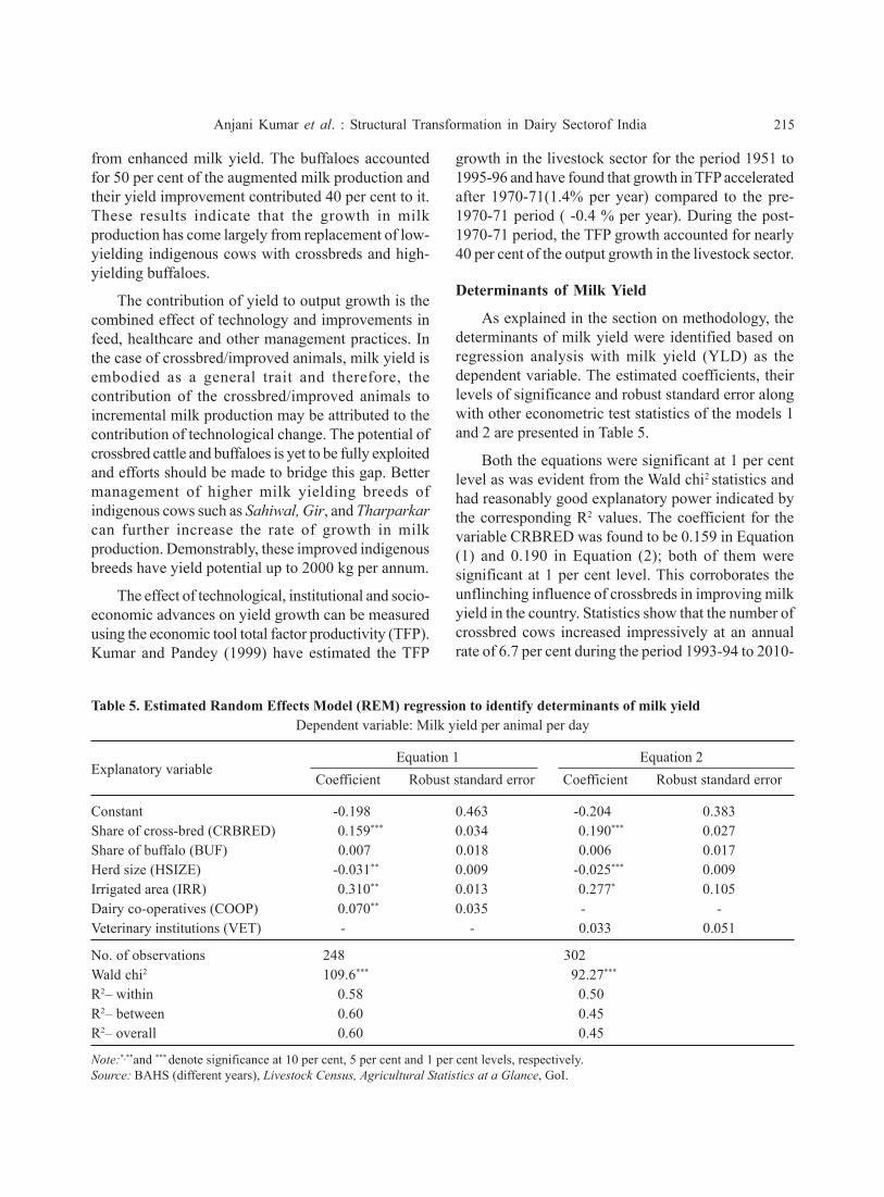
Anjani Kumar et al. : Structural Transformation in Dairy Sectorof India 215
from enhanced milk yield. The buffaloes accountedfor 50 per cent of the augmented milk production andtheir yield improvement contributed 40 per cent to it.These results indicate that the growth in milkproduction has come largely from replacement of low-yielding indigenous cows with crossbreds and high-yielding buffaloes.
The contribution of yield to output growth is thecombined effect of technology and improvements infeed, healthcare and other management practices. Inthe case of crossbred/improved animals, milk yield isembodied as a general trait and therefore, thecontribution of the crossbred/improved animals toincremental milk production may be attributed to thecontribution of technological change. The potential ofcrossbred cattle and buffaloes is yet to be fully exploitedand efforts should be made to bridge this gap. Bettermanagement of higher milk yielding breeds ofindigenous cows such as Sahiwal, Gir, and Tharparkarcan further increase the rate of growth in milkproduction. Demonstrably, these improved indigenousbreeds have yield potential up to 2000 kg per annum.
The effect of technological, institutional and socio-economic advances on yield growth can be measuredusing the economic tool total factor productivity (TFP).Kumar and Pandey (1999) have estimated the TFP
growth in the livestock sector for the period 1951 to1995-96 and have found that growth in TFP acceleratedafter 1970-71(1.4% per year) compared to the pre-1970-71 period ( -0.4 % per year). During the post-1970-71 period, the TFP growth accounted for nearly40 per cent of the output growth in the livestock sector.
Determinants of Milk Yield
As explained in the section on methodology, thedeterminants of milk yield were identified based onregression analysis with milk yield (YLD) as thedependent variable. The estimated coefficients, theirlevels of significance and robust standard error alongwith other econometric test statistics of the models 1and 2 are presented in Table 5.
Both the equations were significant at 1 per centlevel as was evident from the Wald chi2 statistics andhad reasonably good explanatory power indicated bythe corresponding R2 values. The coefficient for thevariable CRBRED was found to be 0.159 in Equation(1) and 0.190 in Equation (2); both of them weresignificant at 1 per cent level. This corroborates theunflinching influence of crossbreds in improving milkyield in the country. Statistics show that the number ofcrossbred cows increased impressively at an annualrate of 6.7 per cent during the period 1993-94 to 2010-
Table 5. Estimated Random Effects Model (REM) regression to identify determinants of milk yieldDependent variable: Milk yield per animal per day
Equation 1 Equation 2Explanatory variable
Coefficient Robust standard error Coefficient Robust standard error
Constant -0.198 0.463 -0.204 0.383Share of cross-bred (CRBRED) 0.159*** 0.034 0.190*** 0.027Share of buffalo (BUF) 0.007 0.018 0.006 0.017Herd size (HSIZE) -0.031** 0.009 -0.025*** 0.009Irrigated area (IRR) 0.310** 0.013 0.277* 0.105Dairy co-operatives (COOP) 0.070** 0.035 - -Veterinary institutions (VET) - - 0.033 0.051
No. of observations 248 302Wald chi2 109.6*** 92.27***
R2– within 0.58 0.50R2– between 0.60 0.45R2– overall 0.60 0.45
Note:*,**and *** denote significance at 10 per cent, 5 per cent and 1 per cent levels, respectively.Source: BAHS (different years), Livestock Census, Agricultural Statistics at a Glance, GoI.

216 Agricultural Economics Research Review Vol. 26 (No.2) July-December 2013
11 at all-India level (Annexure 3). Consequently, therewas a consistent improvement in the quality of milchanimals with resultant gains in milk yield. This findingis consistent with other past studies, such as of Birthalet al., (1999). In contrast, both the coefficientspertaining to the variable, BUF were found to be non-significant.
Another notable finding was the negative andsignificant coefficient for HSIZE in both the equations.Though the herd size in most of the states decreasedover time, evidences suggest that the quality of herdimproved due to replacement of traditional breeds withbetter yielding breeds, with positive outcomes on milkyield. The better management of smaller herds mighthave also contributed towards improving yield levels.The milk yield was also found to improve significantlywith increase in area under irrigation (IRR), which wasa proxy variable for fodder availability. The level ofirrigation has an important role in ensuring year-roundavailability of fodder, thereby augmenting milk yield.Cultivated fodder is an important source of greenfodder, but area under fodder is very limited in thecountry. Presently, only 0.026 ha area per bovine animalis put under fodder crops to meet the fodderrequirement. Therefore, the fodder cultivation shouldbe accorded higher priority and state policies shouldbe tuned to encourage more farmers to take up fodderfarming.
The coefficient pertaining to the variable dairy co-operatives (COOP) was found significant at 5 per centlevel and indicated their influence in improving milkyield through providing better facilities for quality,storage, marketing, processing, and other relatedservices for the dairy farmers. As evident from statistics,the number of dairy co-operatives increasedsubstantially from 63,415 in 1990-91 to 1,44,200 in2010-11 with the associated increase in farmer-members from 7.48 million to 14.46 million and milkprocurement from 3.54 Mt to 9.6 Mt during this period.However, cooperatives have been found workingeffectively only in a few states like Gujarat,Maharashtra, Karnataka, Kerala, Tamil Nadu, etc. andin spite of their tremendous growth, only 10 per centof the dairy farmers could be associated with them.Therefore, efforts are required to spread the success ofdairy co-operatives to more states so that the advantagesof collective action can be harnessed for betterperformance in the sector. While the influence of dairy
cooperatives on milk yield was apparent, the variableVET in Equation (2), denoting the veterinaryinfrastructure, turned out to be non-significant,suggesting inadequacy of the existing veterinaryfacilities in bringing about a perceivable dent in milkyield.
Though yield enhancement in the sector is directlydriven by the factors like share of crossbreds in animalstock, herd size, area under irrigation, dairy co-operatives, etc., as discussed above, the indirectinfluence of dairy infrastructure and other associatedvariables cannot be overlooked. Even though thevariable VET per se had an insignificant contributionin raising the milk yield, its role in supporting theprimary variables was worth examining. For instance,growth in the number of cross-bred cattle and high-yielding buffaloes has depicted a close association withthe number of AI centres, veterinary facilities availableand personnel deployed for providing these services.However, the veterinary infrastructure in the countryhas been found in a poor state of affairs. There is onlyone veterinary institute for nearly 5800 animals (Table6). Further, these institutes do not have adequatenumber of trained veterinary professionals. There isroughly one veterinarian for each veterinary instituteand consequently, a large number of animals do notget veterinary care at appropriate time and place.
Table 6. Status of infrastructure and other variablesrelated to performance of dairy sector
(in No.)
Particulars 1992-93 2010-11
Bovine animals served per 7632 5799veterinary instituteBovine animals per veterinary 9219 5627personTotal AI centres 39600 55806AIs performed per 1000 milch 155 373animalsAdult female bovine per AI centre 2727 1807Bovine breeding farms 183 199Semen production centres 148 172Frozen semen banks 91 184Liquid nitrogen plants 151 91
Source: Basic data from BAHS (different years), Livestock Census,Land Use Statistics, Agricultural Statistics at a Glance, PopulationCensus, GoI.

Anjani Kumar et al. : Structural Transformation in Dairy Sectorof India 217
However, facilities for artificial insemination (AI) aremore abundant than veterinary facilities and there isone AI centre for about 1800 adult female bovines.Thus, about 33 per cent of the animals can be artificiallyinseminated each year. However, because of the lowsuccess rate of AIs, only about 20 per cent of the adultfemales are being inseminated artificially with theexisting infrastructure. A little more than one-fourthof the cows-in-milk are presently crossbred and thedemand for crossbred species is increasing rapidly. Theinfrastructure for developing high-yielding bovines andcross-breds has been found limited. There are onlyabout 200 bovine breeding farms (cattle and buffalo)in the country. The number of semen productioncentres, frozen semen banks, liquid nitrogen plants,etc. is also grossly inadequate. All these facts point tothe vast scope in improving the veterinary infrastructurein the country for realizing better performance. Higherinvestments and appropriate policy support aretherefore required to bring about the perceivable resultsin the area of milk production.
Conclusions and Policy ImplicationsThe study has revealed that India has made
significant strides in enhancing milk production andyield, particularly during the past two decades. Thestructural changes in production of milk have been quitevisible and the composition of dairy animals has tiltedin favour of improved crossbred cattle and better-yielding buffaloes. The role of some new states inaugmenting milk production in India is also apparent.The growth in milk yield has been considerable and isreflected in its contribution to output growth. Morethan half of the growth in milk production during thepast two decades has been contributed by the growthin milk yield. The major determinants of milk yieldinclude technological change and quality of herd,irrigation development, expanding network of dairycooperatives, etc.
Achieving a higher growth in the dairy sector isessential to ensure long-term inclusive agriculturalgrowth. Productivity-led growth is the only viableoption for accelerated and sustainable growth of thesector. The study has pointed out several avenues andstrategies for policy intervention to support dairydevelopment for enhanced milk yield. The analysis hasprovided a strong case for continued investments inimproved breeds of cattle and buffalo. It has been
shown that improved animal species have been criticalto milk yield enhancement. The study has shown anegative relationship between herd size and milk yield,the underlying hypothesis being improvement in herdquality and better management lead to yield growthdespite decrease in herd size. The study has alsobrought out the positive impact of dairy cooperativeson milk yield by facilitating integration between ruralproducers and urban consumers and through fosteringnew technology. However, the status of veterinary andanimal healthcare infrastructure and the delivery ofthese services are still poor and concerted efforts arerequired to bring about further progress. Thestrengthening of market linkages through expansionof cooperatives, and facilitating new models of dairyfarming would go a long way in further improving milkyield in the country.
AcknowledgementThe authors acknowledge the funding support of
IFPRI. The study was conducted at National Centrefor Agricultural Economics and Policy Research(NCAP), New Delhi. They are grateful to Prof. RameshChand, Director, NCAP for providing institutional,infrastructural and intellectual support for conductingthis study.
ReferencesAgricultural Statistics at a Glance (various years)
Directorate of Economics and Statistics, Departmentof Agriculture and Cooperation, Ministry ofAgriculture, Government of India. New Delhi
BAHS (Basic Animal Husbandry and Statistics) (variousyears) Department of Animal Husbandry, Dairying, andFisheries, Ministry of Agriculture, Government of India,New Delhi.
Birthal, P.S. and Negi, D.S. (2012) Livestock for higher,sustainable and inclusive agricultural growth. Economicand Political Weekly, 47(26&27): 89-99.
Chand, Ramesh and Raju, S.S. (2008) Livestock sectorcomposition and factors affecting its growth, IndianJournal of Agricultural Economics, 63(2): 198-210.
FAO (Food and Agriculture Organization) (2003) MilkProduction in India: Opportunities and Risks for SmallScale Producers. PPLPI Policy Brief, Rome.

218 Agricultural Economics Research Review Vol. 26 (No.2) July-December 2013
Jha, Brajesh (2004) India’s Dairy Sector in the EmergingTrade Order. Working Paper No. 243, Institute ofEconomic Growth, New Delhi.
Kumar, Anjani and Pandey, U.K. (1999) Growthperformance of livestock sector in India. In: Sources ofGrowth in the Livestock Sector, Eds: P.S. Birthal, AnjaniKumar, A. Ravishankar and U.K. Pandey Policy Paper9, National Centre for Agricultural Economics andPolicy Research, New Delhi.
Kumar, Anjani, Staal, Steven J., Lapar, Lucy andBaltenweck, Isabelle (2010) Traditional milk marketin Assam: Potential for income and employmentgeneration. Indian Journal of Agricultural Economics,65 (4): 747-59.
DES (Directorate of Economics and Statistics) (variousyears) Land Use Statistics, Department of Agricultureand Cooperation, Ministry of Agriculture, Governmentof India, New Delhi (http://eands.dacnet.nic.in).
DAHD (Department of Animal Husbandry Dairying andFisheries) (various years) Livestock Census, Ministryof Agriculture, Government of India, New Delhi.
Rajendran, K. and Mohanty, S. (2004) Dairy co-operativesand milk marketing in India: Constraints andopportunities. Journal of Food Distribution Research,35 (2): 34-41.
Saikia, T.N. and Kakaty, Gautam (2007) Evaluation of IDDPProject in Operation Flood, Hilly and Backward Areasof North-Eastern Region, Report submitted by Agro-Economic Research Centre for North-East India, AssamAgricultural University, Jorhat, Assam.
Singh, Shiv Raj and Datta, K.K. (2010) Understanding valueaddition in Indian milk sector: Some perspectives.Agricultural Economics Research Review, 23(Conference Number): 487-493.
Revised received: March, 2013; Accepted May, 2013

Anjani Kumar et al. : Structural Transformation in Dairy Sectorof India 219
Annexure 1Mean and standard deviation of explanatory variables (year)
Explanatory variable Mean Standard deviation
Share of cross-bred in milch animal (%) 19.83 21.48Share of buffalo in milch animal (%) 33.03 26.73Herd size (No.) 2.97 3.51Irrigated area (%) 40.33 26.43Dairy co-operative societies (No. per ‘000 bovine units) 0.74 0.72Veterinary institutes& hospitals (No. per ‘000 bovine units) 0.69 1.09
Annexure 2Econometric tests associated with regression and their results
Test Statistic Null hypothesis Model 1 Model 2
Hausman test Chi2 statistic REM preferred over FEM 3.61ns 2.28ns
Breuch Pagan LM test Chibar2 statistic OLS preferred over REM 1233*** 1499***
LR test for heteroscedasticity LR Chi2 statistic Homoscedasticity 275.6*** 388.2***
Wooldridge test for autocorrelation F statistic No first order autocorrelation 5.27** 11.52***
Note: ns denotes non-significant** and *** denote significance at 5 per cent and 1 per cent levels, respectively
Annexure 3Annual growth rate in factors associated with milk yield: 1993-2010
Particulars Trend growth rate (%)
Cross-bred cows 6.74Buffaloes 1.97Herd size (No./household) -0.49Irrigated area (%) 1.32Membership of dairy co-operative societies 2.97Number of veterinary institutes 0.90


Agricultural Economics Research ReviewVol. 26 (No.2) July-December 2013 pp 221-228
Investment in Wheat Research in Nepal – AnEmpirical Analysis§
Hari Krishna Shresthaa*, Hira Kaji Manandharb and Punya Prasad Regmic
aPlanning Division, Nepal Agricultural Research Council, Singhadurbar Plaza, Kathmandu, NepalbPlant Pathology Division, Nepal Agricultural Research Council, Khumaltar, Lalitpur, Nepal
cDepartment of Agricultural Economics, Institute of Agriculture and Animal Science,Tribhuvan University, Rampur, Chitwan, Nepal
Abstract
Investment in wheat research in Nepal has been examined through estimation of full time equivalent ofresearchers on the basis of their time spent on wheat crop research. The information about full timeequivalent was collected through questionnaire survey of the researchers involved in various disciplinesof wheat research. The research investment has been compared with production share in value-termsusing congruency model in the major production domains, such as development regions, eco-zones andenvironments. The model comparing actual production share with full time equivalent of researchers hasrevealed a moderately low congruency percentage indicating discrepancies in research investment acrossproduction domains. On adjusting the production share with both research progress and equity factors atthe same time, the congruency percentage increased in production environments and decreased in eco-zones and geographic regions, highlighting the mismatch in research investments. Some policy measureshave been suggested to mitigate the mismatch in resource allocations to wheat research in Nepal.
Key words: Congruency, equity, full time equivalent, production environment, research investment,wheat research, Nepal
JEL Classification: Q16, Q18
IntroductionWheat is Nepal’s one of the major crops grown in
different agro-ecological zones and environmentsendowed with varied production potentials. It iscultivated on 730 thousand hectares of land and hasthe production of 1.61 million tonnes with productivityof 2229 kg/ha in Nepal (MoAC, 2010). Investment onthe crop research has been a driving force behind
increasing its productivity through varietaldevelopment and improved management practices.Studies in different countries have revealed thatinvestments in agricultural research and development(R&D) have yielded handsome dividends for society,more than enough to justify past investments and tosupport increased funding in the future. The past studieson returns to investment in agriculture have revealedthat the average rate of return per year to be 100 percent for research, 85 per cent for extension, and 48 percent for research and extension taken together (Alstonet al., 2000). The rate of return for investments invarietal development of wheat ranged between 75 percent and 84 per cent during 1960 to 1990 in Nepal(Morris et al., 1994).
*Author for correspondenceEmail: [email protected]
§ The paper has been drawn from PhD thesis entitled,“Resource Allocation in Agricultural Research andDevelopment in Nepal” submitted by the first author toInstitute of Agriculture and Animal Science, TribhuvanUniversity

222 Agricultural Economics Research Review Vol. 26 (No.2) July-December 2013
In order to allocate research resources efficiently,possibilities of advancing knowledge or technologyneed to be explored in a particular commodity, problemor discipline and while the research effort is successful,the likely level of adoption that would occur over agiven time need to be studied (Fuglie, 2007). Type ofresources, partnerships and extension strategies needto be formulated to increase the adoption. In Nepal,research on wheat is mainly carried out by the NepalAgricultural Research Council (NARC), but the R&Dactivities on this crop are also carried out by some non-governmental organizations (NGOs), including theLocal Initiative for Biodiversity, Research andDevelopment (LIBIRD) and Forum for Rural Welfareand Agricultural Reform for Development(FORWARD). Other public organizations such asNepal Academy of Science and Technology (NAST)and Institute of Agriculture and Animal Science (IAAS)of Tribhuvan University also carry out R&D activitiesin addition to their core programs. This study hasanalyzed the investment in wheat research acrossgeographic regions, major agro-ecozones andproduction environments of Nepal. For the study, weconsidered three geographic regions, viz. eastern,central and western and each geographic regionconstituted three major agro-ecozones, viz. terai plains(sub-tropical), hills (warm temperate and sub-tropical),and mountains (temperate), and three major productionenvironments, viz. irrigated, rainfed lowland andrainfed upland.
The public investment in agricultural sector hasbeen about three per cent of the national budget duringthe past three years (2009-2011), although agriculturehas contributed about 32 per cent to the country’s gross
domestic production (GDP). The investment in Nepal’sagricultural research was about 0.26 per cent ofagricultural GDP during the period. This was muchlower than the average expenditure in the developingcountries which was 0.60 per cent of their agriculturalGDP (Pardey and Beintema, 2001). A significantincrease in investment in agricultural research is neededto generate new technologies for future growth inproductivity.
The country employed 33 full time equivalent(FTE) agricultural researchers for every one millionfarmers and invested 520 million Nepalese Rupees or23 million purchasing power parity (ppp) US dollarsin agricultural research at 2005 prices in 2009 (Rahijaet al., 2011). Of the total human resources, 44 per centof the agricultural researchers were focused on crops,22 per cent on livestock, 16 per cent on fisheries and 5per cent on forestry (Rahija et al., 2011).
There is a complex relationship across investmentin agriculture, increase in production and productivity,and levels of rural poverty. Thirtle et al. (2001) haveobserved that an increase in agricultural output couldlead to a reduction in poverty by evidencing 1 per centincrease in total factor productivity (TFP) and loweringthe poverty ratio by 1.3 per cent in Asia. Fan et al.(1999) have found that improvement in TFP andreduction in poverty in India were driven byinvestments in agricultural R&D and infrastructuraldevelopment, particularly roads.
During the past ten years, resource allocation towheat research has shown an erratic pattern of growthin Nepal, although there has been a substantial increasefrom 2010 onwards (Figure 1). The resource allocation
Figure 1. Investment in wheat research: 2000-2012

Shrestha et al. : Investment in Wheat Research in Nepal 223
to wheat research has depicted a trend more or lesssimilar to the overall agricultural research.
This study has investigated whether the researchresources allocated to wheat research matched with theeconomic contribution of this crop in each of thegeographical regions, agro-ecozones and productionenvironments of Nepal.
Data and MethodologyA questionnaire survey was carried out among
wheat researchers associated with differentgovernmental and non-governmental organizations toidentify the full time equivalent (FTE) for their timespent on crop research. The information was collectedfrom 120 researchers of various disciplines who werespending their part or full time on wheat research. Ameasure of FTE in wheat research was used as a proxyfor measurement of investment since the requiredinformation according to production domains such asgeographical regions, ecological zones andenvironments was not available. The FTE is used as acommon measure of research investment based on thetime spent by a researcher on a commodity or discipline(Gauchan and Pandey, 2011; Pandey and Pal, 2007;Stads and Shrestha, 2006).
The various methods used for estimating theallocation of research resources are mostly based oneconomic surplus approach but vary in complexitiesand data requirements. A simple and commonly usedprocedure is based on the congruency approach whichrules that resources should be allocated in proportionto the economic significance that is mostly measuredby the value of production. This rule specifies that theshare of a specific region or environment or commodityin the total research budget should be equal to its sharein the total value of production (Anderson and Parton,1983; Byerlee, 2000). Following Byerlee and Morris(1993) and Pandey and Pal (2007), the congruency wasmeasured as per Equation (1):
C = 1 – Σ (Ri –Vi)2 …(1)
where, 0 ≤ C ≤ 1, with C = 0 indicating no congruencybetween the allocation of research resources and valueof output of a particular commodity. Congruencyincreases as the value of C approaches unity. Ri is theshare of research resources allocated to the commodityi, and Vi is the share of the output value of the samecommodity.
The above congruency approach can be modifiedto incorporate the elements of scoring approach (Alstonet al., 1995; Gyrseels et al., 1992; Barker, 1988). Inthe present study, the index of output value in eachdomain was adjusted by weighting the value ofproduction based on two factors, viz. research progressand poverty ratio. The first factor consisted ofefficiency criterion relating the expected returns fromcommodity research expenditures which was termedas ‘expected research progress’. The second factorconsisted of an equity criterion relating to the expecteddistributional effects of technical change which wastermed as ‘poverty incidence’. Some more explanationon these factors is given below.
Rate of Expected Research Progress
The progress in wheat research in favourableenvironment differs from that in unfavourableenvironment. The expected rate of research progressneeds to be adjusted in actual production share in orderto modify the future research allocation. The pastresearches have been successful in increasingproductivity in the irrigated areas, but the success wasless in the rainfed areas, as witnessed in the impact ofgreen revolution. A modest productivity growth in thepast reflected a low level of resource allocation inagriculture. The likelihood of future progress issignificant in guiding the ex-ante allocation ofresources.
To estimate productivity growth and futureresearch progress, experienced agronomists andbreeders of Nepal were consulted. Their estimation wasbased on high-yielding pipeline technologies in wheatfor different environments or eco-zones.
Incidence of Poverty
To compare resource allocation to wheat researchacross different environments, poverty ratio was used.One of the major justifications for investing in researchtargeted at crops in marginal environments is the higherincidence of poverty in these environments.
Data on poverty ratio were available only forpolitically-defined areas such as districts anddevelopment regions. Mountainous districts comprisemostly marginal land with low productivity resultingin high poverty ratio and high vulnerability to foodsecurity. Hilly districts have relatively more productive

224 Agricultural Economics Research Review Vol. 26 (No.2) July-December 2013
land and show less vulnerability to food security. Theterai districts have most favourable and productive landand depict low poverty ratio. Since the data on povertyratio were not available according to environments,these were estimated based on their agriculturalproductivity.
Results and Discussion
Resource Allocation to Wheat Research
The total number of researchers involved in wheatwas 28 full time equivalents (FTE) in 2011 (Table 1).The operational cost in wheat research was US$ 278thousand at current price which is equivalent to US$9942 per FTE researcher. In the case of rice, Gauchanand Pandey (2011) have found US$ 5,930 per FTE ofrice researcher in 2009 in Nepal. The investment perFTE researcher in rice in India was estimated to beUS$ 15780 for eastern India and US$ 21,110 for therest of India in 2000 (Pandey and Pal, 2007).
Of the total wheat area (730 thousand ha), 63 percent was irrigated with average yield of 2471 kg/ha,and the remaining area was rainfed with average yieldof 1074 kg/ha (MoAC, 2010). Across the eco-zones,terai plains comprised 58 per cent of the total wheatarea with 49 per cent of FTE share, indicating asubstantial proportion of underinvestment. Hill eco-zone comprised 35 per cent of the total wheat area with47 per cent of FTE share that indicated a substantiallevel of overinvestment. Mountain eco-zone comprisedabout 7 per cent of the total wheat area with a share of4 per cent in FTE, indicating underinvestment(Table 1). The mismatch of investment in wheatresearch might have resulted from the irrationalresource allocation and inefficiency of researchmanagement.
Congruency Analysis across Eco-zones
The congruency between actual production shareand FTE share was 92 per cent indicating a moderatelevel of under-investment in wheat research acrossdifferent ecological zones (Table 2). The actualproduction share was 20 points higher than the FTEshare in the terai plains, whereas it was lower than theFTE share by a similar magnitude in the hills. In themountains, the actual production share was least butexactly equalled to FTE share, indicating a perfectbalanced investment. The results revealed that wheatresearch in the hills was over-invested on the basis ofcontribution of hill eco-zone to the total productionvalue. The terai plains had a relatively larger share intotal production but this eco-zone had beenunderinvested for wheat research.
One of the important reasons behind theoverinvestment in the hills is that the divisions of thesedisciplines are located in the Kathmandu valley, whichis in the hill eco-zone. However, the issue of over-investment could be overlooked because these divisionscarry out research work not only for hills but formountains and terai plains also.
Based on the experience and knowledge of wheatresearchers, the expected increase in wheat productivityin the next ten years was estimated as 20 per cent inthe terai and 10 per cent each in the hills and themountains. The terai belt of Nepal has higher potentialof productivity increase due to relatively good soilfertility and availability of abundant water forirrigation. In another study, the expected yield gainsin rice relative to the current values were estimated as30 per cent for the terai, 20 per cent for the hills, and10 per cent for the mountains (Gauchan and Pandey,2011). The poverty ratios for the mountains and thehills were estimated to be 10 per cent and 15 per cent
Table 1. Full time equivalent (FTE) in wheat research across different eco-zones and environments in Nepal
Environment Eco-zones
Full time equivalent (FTE) Area (% share)
Terai Hills Mountains Terai Hills Mountains
Irrigated 8.00 7.00 0.50 46.15 14.74 2.50Rainfed lowland 4.24 5.00 0.50 12.01 18.58 3.85Rainfed upland 1.50 1.15 0.15 0.09 1.66 0.42Total 13.74(49%) 13.15(47%) 1.15(4%) 58.25 34.98 6.77

Shrestha et al. : Investment in Wheat Research in Nepal 225
higher, respectively than for the terai plains. We usedthe poverty weight 1 for the terai, 1.15 for the hills and1.10 for the mountains. The Nepal Living StandardSurvey (NLSS) of 2003-04 has shown that the povertyrate is lowest in the terai region than in the mountainsand the hills (CBS, 2005). While we have adjusted theactual production share with the rate of expectedresearch progress alone, the congruency percentagedeclined by 2 points. In contrast, the congruencypercentage increased by the same magnitude when theproduction share was adjusted with equity factor forpoverty consideration. When the production share wasfully adjusted with both the factors, the congruencyhad declined by 7 points, amplifying the mismatch ofinvestment across different eco-zones.
Congruency Analysis across the Environments
When FTE share and actual production share wereanalyzed for three production environments, viz.irrigated, rainfed lowland and rainfed upland, thecongruency was found to be 91 per cent (Table 3). Thisindicated a moderate level of underinvestment in wheatresearch across different environments in Nepal. Theactual production share was 25 points higher than theFTE share of irrigated environments, whereas it was12 points lower than the FTE share of rainfed lowlandand 13 points lower than the FTE share of rainfedupland. It indicated a discrepancy in investment in theseproduction environments with empirical evidence ofunderinvestment in the irrigated environment andoverinvestment in the rainfed environment. The actualpattern of wheat research across the productionenvironments has shown an overall congruency of 92per cent in India and 96 per cent in CIMMYT membercountries (Byerlee and Morris, 1993). The congruency
in rice research in India was as high as 99 per centacross different environments of the country (Pandeyand Pal, 2007).
The research emphasis on rainfed wheat might bedue to the present scenario of climate change thatcompelled to invest in resource conservationtechnologies to cope-up with unfavourableenvironment. Although the production share of rainfedenvironment is low at present, push-up in investmentis required for the long-run production growth andpoverty reduction in such a marginal area. However,the importance of according highest weight to favouredenvironments is supported by the evidence that thereare significant positive spillover effects fromtechnological change in these environments whichultimately benefit the poor in marginal environmentsthrough lower food prices, increased employment andhigher wages (David and Otsuka, 1992). Thesespillover effects may actually exceed the positivebenefits generated through research targetedspecifically at marginal environments (Renkow, 1991).
The future progress in wheat research has beenestimated to be 15 per cent in the irrigated environment,30 per cent in the rainfed lowland, and 20 per cent inthe rainfed upland environments. The reason behindthe modest future productivity growth in irrigatedenvironment is the current higher yield due to relativelyhigh use of inputs in these environments. The potentialof yield increase in the rainfed lowland is more becauseof the upcoming water-saving technology which ishighly suitable in this environment. The irrigatedenvironment received high priority during the greenrevolution period primarily because of its high growthpotential. This paid rich dividends in terms of quantumjump in crop yields, but in the process, rainfed and
Table 2. Full time equivalent (FTE) of researchers and share of wheat production across eco-zones in Nepal
Eco-zonesParameters Terai Hills Mountains All Congruency
FTE 13.74 13.15 1.15 28.04FTE share 49.00 47.00 4.00 100.0Actual production share 69.37 26.63 4 100.0 0.92Adjusted production share (research progress) 71.19 25.05 3.76 100 0.90Adjusted production share (equity) 66.45 29.34 4.21 100.0 0.94Fully adjusted production share (research progress 77.57 20.93 1.50 100.0 0.85and equity)

226 Agricultural Economics Research Review Vol. 26 (No.2) July-December 2013
marginal regions were neglected (Pal and Singh, 1997).The poverty ratio was estimated to be 30 per cent higherin the rainfed lowland and 50 per cent higher in therainfed upland as compared to in irrigated environment.The estimated poverty ratio was based on the wheatproductivity which varied widely across differentenvironments. The average wheat yield with improvedvariety was 2471 kg/ha in the irrigated condition, and1074 kg/ha in the rainfed lowland. The average wheatyield of local variety in rainfed upland was 752 kg/ha(MoAC, 2010).
When the actual production share was adjustedwith the expected research progress, the congruencyindex had increased by only one per cent. When theactual production share was adjusted with equity factor,the congruency index inclined to 94 per cent. Thecongruency index increased up to 97 per cent whenthe actual production share was adjusted with both thefactors (Table 3).
Congruency Analysis across the GeographicRegions
The western region of Nepal had the highestproduction share (51%) in the total wheat productiondespite its lower FTE share of 36.5 per cent (Table 4).Since the western region comprised the largest wheatarea and had potential of a significant increase in yield,the resource allocation to wheat research need to beincreased substantially in this region. Also, an incentivemechanism should be developed for motivation ofresearchers to work consistently in the region.
The gap between potential yield and on-farm yieldof wheat was higher in the western than in the easternand central regions. Based on the potentiality ofpipeline technologies, the wheat productivity wasanticipated to increase by 10 per cent each in the easternand central regions and by 20 per cent in the westernregion in the next ten years. It was because the soil of
Table 3. Full time equivalent (FTE) and share of wheat production across different production environments inNepal
EnvironmentParameters Irrigated Rainfed lowland Rainfed upland All Congruency
FTE 15.55 7.74 4.75 28.04FTE share 55.00 28.00 17.00 100.0Actual production share 80.00 16.00 4.00 100.0 0.91Adjusted production share 78.23 17.69 4.08 100.0 0.92(research progress)Adjusted production share 74.91 19.48 5.62 100.0 0.94(equity)Fully adjusted production share 47.25 41.66 11.09 100.0 0.97(research progress and equity)
Table 4. Full time equivalent (FTE) and share of wheat production across different geographical regions of Nepal
Parameters Eastern region Central region Western region All regions Congruency
FTE 2.40 15.39 10.25 28.04FTE share 8.50 55.00 36.50 100.0Actual production share 16.00 33.00 51.00 100.0 0.92Adjusted production share 15.29 31.54 53.17 100.0 0.91(research progress)Adjusted production share (equity) 15.05 28.23 56.72 100.0 0.88Fully adjusted production share 11.07 20.74 68.19 100.0 0.78(research progress and equity)

Shrestha et al. : Investment in Wheat Research in Nepal 227
western region has not been exploited with higherinputs as compared to in the eastern and central regions.Poverty ratio was estimated to be higher in the easternand western regions by 10 per cent and 30 per cent,respectively as compared to that in the central region.It was because the central region had a better access toinputs and market, thereby increasing incomegeneration activities of the farmers. The average farmyield was 2122 kg/ha in the eastern region, 1608 kg/ha in the far western region and 2322 kg/ha in thecentral region (MoAC, 2010).
ConclusionsThe congruency index with actual production share
has indicated moderate discrepancies in researchinvestment in wheat in all the production domains ofNepal. The wheat research has been found over-invested in the hills, and rainfed environments andunder-invested in the terai plains and irrigatedconditions. Across geographic regions, the centralregion has been observed to be over-invested whereaseastern and western regions are under-invested. Whenthe production share was adjusted with researchprogress and equity factors, the congruency percentageincreased in some cases and declined in other cases. Ahigher investment is required for wheat research in theirrigated environment as well as in terai plains. Thewestern region also needs substantial increment inresearch investment since it has the largest contributionto the total value of wheat production. Although theissue of mismatch in the allocation of researchresources across the production domains is important,it is even more important to raise the investment in theagricultural research system in Nepal.
AcknowledgementsThe authors are grateful to International Rice
Research Institute (IRRI), Manila, for providingfinancial support to conduct this study as a partialfulfillment of PhD thesis on ‘Resource Allocation inAgriculture Research in Nepal’. They thank Dr SushilPandey of IRRI for his generous support and technicalguidance. They are also thankful to Dr DevendraGauchan, Nepal Agricultural Research Council andDr Bhaba Tripathi, IRRI-Nepal office, for theirsupport during the study. They thank the anonymousreferee for the critical comments which helped on thispaper.
ReferencesAlston, J.M., Norton, G.W. and Pardey, P.G. (1995) Science
under Scarcity: Principles and Practice for AgriculturalResearch Evaluation and Priority Setting. CornellUniversity Press, Ithaca, New York.
Alston, J.M., Chan-Kang, C., Marra, M.C., Pardey P.G. andWyatt, T.J. (2000) A Meta-Analysis of Rates of Returnto Agricultural R&D ex pede herculem? InternationalFood Policy Research Institute, Washington DC.
Anderson, J.R. and Parton, K.A. (1983) Techniques forguiding the allocation of resource among rural researchprojects: State-of-the-art. Prometheus, 1: 180-201.
Barker, R. (1988) Methods for setting agricultural researchpriorities in Report of a Bellagio Conference. Workingpaper No. 88-3. Department of Agricultural Economics,Cornell University, Ithaca, New York.
Byerlee, D. and Morris, M. (1993) Research for marginalenvironments: Are we under-invested? Food Policy, 18:381-393.
Byerlee, D. (2000) Targeting poverty alleviation in prioritysetting for agricultural research. Food Policy, 25: 429-445.
CBS (Central Bureau of Statistics) (2005) Nepal LivingStandard Survey (NLSS) 2003-04. National PlanningCommission, Kathmandu.
David, C. and Otsuka, K. (1992) The green revolution andincome distribution across production environments inAsia. Paper presented at the Rice Research Seminar,IRRI, Los Banos, Philippines.
Fan, S., Hazell, P. and Thorat, S. (1999) Linkages betweenGovernment Spending, Growth and Poverty in RuralIndia. IFPRI research report 110. International FoodPolicy Research Institute. Washington, DC.
Fuglie, K. (2007) Research Priority Assessment for the CIP2005-2015 Strategic Plan: Projecting Impacts onPoverty, Employment, Health and Environment.International Potato Center (CIP), Lima, Peru.
Gauchan D. and Pandey, S. (2011) Is investment in riceresearch in Nepal adequate and balanced acrossproduction environments? Some empirical evidence.Quarterly Journal of International Agriculture, 50(4):305-324.
Gyrseels, G., De Wit, C.T., McCalla, A., Monyo, J., Kassam,A.H., Craswell, E. and Collinson, M. (1992) Settingagricultural research priorities for the CGIAR.Agricultural System, 40: 59-103.
228 Agricultural Economics Research Review Vol. 26 (No.2) July-December 2013
MoAC (Ministry of Agriculture and Cooperatives) (2010)Statistical Information on Nepalese Agriculture.Kathmandu, Nepal.
Morris, M.L, Dubin, H.J. and Pokhrel, T. (1994) Returns towheat breeding research in Nepal. AgriculturalEconomics, 10: 269-282.
Pal, S. and Singh, A. (1997) Agricultural Research andExtension in India: Institutional Structure andInvestments. Policy Paper 7. National Centre forAgricultural Economics and Policy Research, NewDelhi.
Pandey, S. and Pal, S. (2007) Are less-favored environmentsover-invested? The case of rice research in India. FoodPolicy, 32: 606-623.
Pardey, P.G. and Beintema, N.M. (2001) Slow Magic:Agricultural Research a Century after Mendel.International Food Policy Research Institute,Washington DC.
Rahija, M., Shrestha, H.K., Stads, G.J. and Bhujel, R.B.(2011) Recent Development in Public Agricultural
Research. Agricultural Science and TechnologyIndicators: Nepal. International Food Policy ResearchInstitute, Washington DC.
Renkow, M. (1991) Modeling the Aggregate Effects ofTechnological Change on Income Distribution inPakistan’s Favored and Marginal ProductionEnvironments. Economics Paper No. 4. CIMMYT,Mexico.
Stads, G.J. and Shrestha, H.K. (2006) Agricultural Scienceand Technology Indicators: Nepal. ASTI country briefNo. 37. International Food Policy Research Institute,Washington DC.
Thirtle, C., Xavier, I., Lin, L., McKenzie-Hill, V. andWiggins, S. (2001) Relationships between changes inAgricultural Poverty in Developing Countries. DFIDreport 7946. Department for International Development,London.
Received: January, 2013; Accepted June, 2013

Agricultural Economics Research ReviewVol. 26 (No.2) July-December 2013 pp 229-239
Agricultural Price Forecasting Using Neural Network Model: AnInnovative Information Delivery System
Girish K. Jha*a and Kanchan Sinhab
aIndian Agricultural Research Institute, New Delhi – 110 012bIndian Agricultural Statistics Research Institute, New Delhi – 110 012
Abstract
Forecasts of food prices are intended to be useful for farmers, policymakers and agribusiness industries.In the present era of globalization, management of food security in the agriculture-dominated developingcountries like India needs efficient and reliable food price forecasting models more than ever. Sparse andtime lag in the data availability in developing economies, however, generally necessitate reliance on timeseries forecasting models. The recent innovation in Artificial Neural Network (ANN) modellingmethodology provides a potential price forecasting technique that is feasible given the availability ofdata in developing economies. In this study, the superiority of ANN over linear model methodology hasbeen demonstrated using monthly wholesale price series of soybean and rapeseed-mustard. The empiricalanalysis has indicated that ANN models are able to capture a significant number of directions of monthlyprice change as compared to the linear models. It has also been observed that combining linear andnonlinear models leads to more accurate forecasts than the performances of these models independently,where the data show a nonlinear pattern. The present study has aimed at developing a user-friendly ANNbased decision support system by integrating linear and nonlinear forecasting methodologies.
Key words: Hybrid model, neural networks, price forecasting, agriculture
JEL Classification: Q16, Q15
IntroductionPrice forecasting is an integral part of commodity
trading and price analysis. Quantitative accuracy withsmall errors, along with turning point forecasting poweris important for evaluating forecasting models.Agricultural commodity production and prices are oftenrandom as they are largely influenced by eventualitiesand are highly unpredictable in case of naturalcalamities like droughts, floods, and attacks by pestsand diseases. This leads to a considerable risk anduncertainty in the process of price modelling andforecasting. Agricultural commodity prices play animportant role in consumers’ access to food as they
directly influence their real income, especially amongthe poor who spend a large proportion of their incomeon food. Since food price is an important componentto fight hunger, policymakers need reliable forecastsof expected food prices in order to manage foodsecurity. Before the onset of liberalization andglobalization, the government was controlling foodprices, thus rendering food price forecasting a lowvalue-added activity. Presently, the food prices aredetermined by the domestic and international marketforces. This leads to increased price variability, andaccords importance to reliable price forecastingtechniques. The price forecasts are important forfarmers also as they base their production andmarketing decisions on the expected prices that mayhave financial repercussions many months later.
*Author for correspondenceEmail: [email protected]

230 Agricultural Economics Research Review Vol. 26 (No.2) July-December 2013
Agricultural Price and Time Series ModellingAgricultural price modelling is different from
modelling of non-farm goods and services due tocertain special features of agricultural product markets.The characteristic features of agricultural crops includeseasonality of production, derived nature of theirdemand, and price-inelastic demand and supplyfunctions. The biological nature of crop productionplays an important role in agricultural product pricebehaviour.
There are two basic approaches of forecasting,namely structural and time series models. The structuralmodels proceed from the first principles of consumerand producer theory to identify the demand and supplyschedules and the equilibrium prices resulting fromtheir intersection. The structural modelling techniquesprovide valuable insights into the determinants ofcommodity price movements. The computational anddata demands of structural price forecasting generallyfar exceed than what are routinely available in thedeveloping countries. Consequently, researchers oftenrely on parsimonious representations of price processesfor their forecasting needs. Contemporaryparsimonious form of price forecasting relies heavilyon time series modelling. The time series modellingrequires less onerous data input for regular and up-to-date price forecasting.
In time series modelling, past observations of thesame variable are collected and analyzed to develop amodel describing the underlying relationship. Duringthe past few decades, much effort has been devoted tothe development and improvement of time seriesforecasting models. One of the most important andwidely used time series models is the Auto RegressiveIntegrated Moving Average (ARIMA) model. Thepopularity of ARIMA model is due to its statisticalproperties as well as use of well-known Box-Jenkinsmethodology in the model building process.
Recently, Artificial Neural Network (ANN)modelling has attracted much attention as an alternativetechnique for estimation and forecasting in economicsand finance (Zhang et al., 1998; Jha et al., 2009). ANNis a multivariate non-linear non-parametric data drivenself-adaptive statistical method. The main advantageof neural network is its flexible functional form anduniversal functional approximator. With ANN, thereis no need to specify a particular model form for a given
data set. ANN has found applications in fields likebiology, engineering, economics, etc. and its use ineconomics has been surveyed by Kuan and White(1994).
Rationale of Research IssueVery few studies have been undertaken on
agriculture price forecasting using ANN models.Moreover, the value of neural network models inforecasting economic time series, has been establishedfor developed countries like USA, Canada, Germany,etc., but little work has been undertaken for developingcountries in general and India in particular. Literaturesuggests that the performance of a non-linear modelshould be evaluated on the basis of percentage offorecasts that correctly predict the direction of changeinstead of measures based on error-terms. Theprediction of turning point is more crucial for anycommodity price forecasting. Lastly, as agriculturalprice data often contain both linear and nonlinearpatterns, no single model is capable to identify all thecharacteristics of time series data on agricultural prices.Obviously, there is a need to examine the priceforecasting performance of hybrid model which takesadvantage of the unique strength of both linear ARIMAmethod and nonlinear ANN model.
The above facts motivated us to assess theforecasting accuracy of neural network model andtraditional statistical models for agricultural priceforecasting using real price data by taking into accountthe major limitations of previous studies. This paperhas summarized the experience of forecasting price anddirection of change using ANN model with twomonthly wholesale oilseeds price series compared toother approaches, where one series was linear and theother was nonlinear in nature. An attempt has also beenmade to discuss opportunities and advantages of softcomputing based decision support system inagricultural price forecasting.
Methodology
Neural Network Model
The time series data can be modelled using ANNby providing the implicit functional representation oftime, whereby a static neural network like multilayerperceptron is bestowed with dynamic properties

Jha and Sinha : Agricultural Price Forecasting Using Neural Network Model 231
(Haykin, 1999). A neural network can be made dynamicby embedding either long-term or short-term memory,depending on the retention time, into the structure of astatic network. One simple way of building short–termmemory into the structure of a neural network isthrough the use of time delay, which can beimplemented at the input layer of the neural network.An example of such an architecture is a Time-DelayNeural Network (TDNN) (Figure 1), which has beenemployed in the present study.
The ANN structure for a particular problem in timeseries prediction includes the determination of numberof layers and total number of nodes in each layer. It isusually determined through experimentation as thereis no theoretical basis for determining these parameters.It has been proved that neural networks with one hiddenlayer can approximate any non-linear function given asufficient number of nodes at the hidden layer andadequate data points for training. In this study, we haveused neural network with one hidden layer. In timeseries analysis, the determination of number of inputnodes which are lagged observations of the samevariable plays a crucial role as it helps in modellingthe autocorrelation structure of the data. Thedetermination of number of output nodes is relativelyeasy. In this study, one output node has been used.Multi-step ahead forecasting is performed usingiterative procedure following Box-Jenkins ARIMA
Time Series modelling methodology. This involves useof forecast value as an input for forecasting the futurevalue. It is always better to select the model with asmaller number of nodes in the hidden layer as itimproves the out-of-sample forecasting performanceand also avoids the problem of over-fitting. The generalexpression for the final output value yt+1 in a multi-layer feed forward time delay neural network is givenby Equation (1):
...(1)
where, f and g denote the activation function at thehidden and output layers, respectively; p is the numberof input nodes (tapped delay); q is the number of hiddennodes; βij is the weight attached to the connectionbetween ith input node to the jth node of hidden layer;αj is the weight attached to the connection from the jth
hidden node to the output node; and yt-i is the ith input(lag) of the model. Each node of the hidden layerreceives the weighted sum of all the inputs, includinga bias term for which the value of input variable willalways be one. This weighted sum of input variablesis then transformed by each hidden node using theactivation function f which is usually a non-linearsigmoid function. In a similar manner, the output nodealso receives the weighted sum of the output of all thehidden nodes and produces an output by transformingthe weighted sum using its activation function g. In
Figure 1. Time-Delay Neural Network (TDNN) with one hidden layer

232 Agricultural Economics Research Review Vol. 26 (No.2) July-December 2013
the time series analysis, f is often chosen as the LogisticSigmoid function and g, as an identity function. Thelogistic function is expressed as Equation (2):
...(2)
For p tapped delay nodes, q hidden nodes, oneoutput node and biases at both hidden and output layers,the total number of parameters (weights) in a three layerfeed forward neural network is q(p + 2) + 1.
For a univariate time series forecasting problem,the past observations of a given variable serve as inputvariables. The TDNN model attempts to map thefollowing function:
...(3)
where, yt+1 pertains to the observation at time t+1, p isthe number of lagged observation, w is the vector ofnetwork weights, and εt+1 is the error-term at time t+1.Hence, TDNN acts like a non-linear autoregressivemodel. The neural network toolbox of MATLAB 7.10software was used to carry out computation relating toTDNN model.
The ARIMA Model
In an Auto-Regressive Integrated Moving Average(ARIMA) model, time series variable is assumed to bea linear function of the previous actual values andrandom shocks. In general, an ARIMA model ischaracterized by the notation ARIMA (p, d, q), wherep, d and q denote orders of Auto-Regression (AR),Integration (differencing) and Moving Average (MA),respectively. ARIMA is a parsimonious approach whichcan represent both stationary and non-stationaryprocesses.
An ARMA (p, q) process is defined by Equation(4):
... (4)
where, yt and εt are the actual value and random errorat time period t, respectively, Φi (i=1, 2,……,p) andφi (j=1, 2,……,q) are the model parameters. Therandom errors, εt are assumed to be independently andidentically distributed with a mean of zero and aconstant variance of σ2.
The first step in the process of ARIMA modellingis to check for the stationarity of the series as theestimation procedure is available only for a stationaryseries. A series is regarded stationary if its statisticalcharacteristics such as the mean and the autocorrelationstructures are constant over time. The stochastic trendof the series is removed by differencing, whilelogarithmic transformation is employed to stabilize thevariance. After appropriate transformation anddifferencing, multiple ARMA models are chosen onthe basis of Auto-Correlation Function (ACF) andPartial Auto- Correlation Function (PACF) that closelyfit the data. Then, the parameters of the tentative modelsare estimated through any non-linear optimizationprocedure such that the overall measure of errors isminimized or the likelihood function is maximized.Lastly, diagnostic checking for model adequacy isperformed for all the estimated models through the plotof residual ACF and using Portmonteau test. The mostsuitable ARIMA model is selected using the smallestAkaike Information Criterion (AIC) or Schwarz-Bayesian Criterion (SBC) value and the lowest rootmean square error (RMSE). In this study, all estimationsand forecasting of ARIMA model have been done usingSAS/ETS 9.2.
The Hybrid ARIMA - TDNN Methodology
In this section, the time series decomposition isproposed in which ARIMA and TDNN models arecombined in order to obtain a robust and efficientmethodology for time series forecasting. Accordingly,we postulate that our time series data can bedecomposed into a linear and a nonlinear component(Rojas et al., 2008), viz.
…(5)
where, yt is the observed time series data, Lt is the linearauto-regressive component, and Nt is the non-linearcomponent. In this approach, we apply an ARIMAmodel to the data series to fit the linear part and theresiduals are modelled using neural network modelonly if there is an evidence of non-linearity for theseries. Figure 2 shows a schematic diagram of thismethod. Let rt be the residual at time t of the linearcomponent, then
…(6)

Jha and Sinha : Agricultural Price Forecasting Using Neural Network Model 233
where, L^t is the estimate of the linear auto-regressivecomponent. For non-linear components, we applyneural network model, i.e.
…(7)
where, p is the number of input delays and f is thenonlinear function. So the combined forecast is givenby Equation (8):
…(8)
where, εt is the error-term of the combined model attime t. Here, it is assumed that since ARIMA modelcannot capture the nonlinear structure of the data, theresidual of linear model will contain information aboutnonlinearity. Hence, the hybrid architecture is expectedto exploit the feature and strength of both the modelsin order to improve the overall forecastingperformance.
In this study, the McLeod and Li test (1983) hasbeen applied to detect non-linearity in the data. Thistest is based on the autocorrelations of the squaredresiduals. In this test, the residuals which are obtainedfrom fitted ARIMA model are utilized to test non-
linearity. The test statistic is given by Equation(9):
…(9)
where, r(i) is the autocorrelation of the squaredresiduals, and h is the number of autocorrelations.
Forecast Evaluation Methods
The forecasting ability of different models isassessed with respect to two common performancemeasures, viz. the root mean squared error (RMSE)and the mean absolute deviation (MAD). The RMSEmeasures the overall performance of a model and isgiven by Equation (10):
…(10)
where, yt is the actual value for time t, y^t is the predictedvalue for time t, and n is the number of predictions.The second criterion, the mean absolute deviation is ameasure of average error for each point forecast and isgiven by Equation (11):
…(11)
where the symbols have the same meaning as above.
Data
This paper has used the monthly average wholesale(nominal) price (rupees per quintal) of two major cropsof oilseeds in India, viz. soybean and rapeseed-mustard,traded in the Indore (Madhya Pradesh) and Delhimarkets, respectively, to evaluate the prediction abilityof different models. The data on soybean were obtainedfrom the website of the Soybean Processors Associationof India (SOPA), Indore, and on rapeseed-mustard werecollected from various issues of Agricultural Prices inIndia, published by the Directorate of Economics andStatistics, Government of India, New Delhi. The priceseries on soybean covered a period of 228 months(October, 1991 to September, 2010) and on rapeseed-mustard covered a period of 372 months (January, 1980to December, 2010). These series illustrate thecomplexity and variation of typical agricultural pricedata (Figure 3). These prices were deflated using thewholesale price index data (2004-05=100) of oilseeds
Figure 2. Hybrid method that combines both ARIMAand TDNN models

234 Agricultural Economics Research Review Vol. 26 (No.2) July-December 2013
estimated by the Office of Economic Advisor, Ministryof Commerce & Industry, Government of India. Thebasic characteristics of the price series used in the studyare presented in Table 1.
Empirical Results and Discussion
Data Preprocessing
The data preprocessing refers to analyzing andtransforming the input and output variables to minimizenoise, highlight important relationships, detect trends,and flatten the distribution of variables to assist bothtraditional and neural network models in the relevantpattern. The first step in time series analysis is to plotthe data. Figure 3 shows the time series plot of averagemonthly price of rapeseed-mustard from January 1980to December 2010. A perusal of Figure 3 reveals apositive trend over time which indicates the non-stationary nature of series. A similar trend was observedin the case of soybean also.
In this study, we have applied the natural choiceof logarithmic transformation to the data to stabilizethe variance. The logarithmic transformation is usedfor the data which can take both small and large valuesand is characterized by an extended right hand taildistribution. The logarithmic transformation is one ofthe data processing techniques which also convertsmultiplicative or ratio relationship to additive whichis believed to simplify and improve neural networktraining. We have applied the Augmented Dickey Fuller(ADF) test for each level and transformed series to testfor the unit root and the results have been presented inTable 2. The values in Table 2 clearly show the non-stationarity of level and transformed series. Therefore,we have used first differencing for both the price series.The first differenced series were found to be stationaryin both cases as indicated in Table 2 and hence furtherdifferencing was not required. The ACF and PACF ofdifferent series have not shown a strong and consistentseasonal pattern.
Table 1. Descriptive statistics of price series used in the study
Crop Minimum Maximum Mean Standard deviation Skewness Kurtosis(`/q) (`/q) (`/q) (`/q)
Soybean 646 2680 1256 472 1.21 3.74Rapeseed-mustard 370 3175 1288 741 0.85 3.02
Figure 3. Rapeseed-mustard monthly price data from January 1980 to December 2010 (`̀̀̀̀/q)

Jha and Sinha : Agricultural Price Forecasting Using Neural Network Model 235
Nonlinearity Test
For choosing the technique for modelling andprediction of data, it is important to find whether agiven time series is non-linear or not. If there is anevidence of nonlinearity in the dynamics underlyingthe data generating process, then nonlinear modelsshould be tried in addition to linear models forforecasting the data. This also enables us to examinewhether nonlinearity tests provide any reliable guidefor post sample forecast accuracy of neural networkmodel. In this study, we have applied McLeod and Linonlinearity test to the data set. It tests the nullhypothesis of linearity against different types ofpossible nonlinearity and is based on theautocorrelations of squared residuals. In this study,autocorrelations up to 24 lags have been used forcomputing the test. The results of McLeod and Li non-linearity test presented in Table 3, reveal strongrejection of linearity in the case of rapeseed-mustardonly. In other words, the analysis has indicated theexistence of some hidden structure left unaccountedin the residuals of linear model in the case of rapeseed-mustard. Based on this evidence, we have suggestedsuitability of nonlinear model for price forecasting ofrapeseed-mustard.
Neural Network and ARIMA Model
For developing a model, we have divided the datainto two sets, viz. training set and testing set. The lasttwelve months price data were retained for testing. The
training set was used for modelling procedure and in-sample prediction and testing set was kept for post-sample forecasting. The training set for the soybeanand rapeseed-mustard series contained 216 and 360observations, respectively. After logarithmictransformation, each series was differenced to make itstationary as price data are trended and nonstationaryin nature. Then, we modelled the relative change inthe price series which also had a meaningful economicinterpretation.
We have found the ARMA structure of differencedseries, based on the autocorrelation function (ACF),partial autocorrelation function (PACF) and AICinformation criterion. We obtained the best ARIMAmodel for each series based on the lowest AIC andBIC information criteria as well as the lowest RMSEand MAD values. We selected the ARIMA (1, 1, 0) forsoybean and ARIMA (2, 1, 0) for rapeseed-mustardseries. Due importance was given to the well-behavedresiduals while selecting the best model.
We have found the best time delay neural networkwith single hidden layer for this study. Following theprevious studies, the logistic and identity functions wereused as activation function for the hidden nodes andoutput node, respectively. We have focused primarilyon the one-step-ahead forecasting and the multi-step-ahead forecasting was done using the iterativeprocedure; so only one output node was employed.Hence, the model uncertainty was associated only withthe number of tapped delays (p) which was the numberof lagged observations in this case and the number ofhidden layer nodes (q). The number of tapped delayand hidden nodes were determined throughexperimentation. We have used multiple starts, withdifferent random starting points, in order to avoid localminima and find the global minimum. In particular,based on the training sample, we have trained each
Table 2. Augmented Dickey-Fuller stationarity test for different series
Null hypothesis Level series Logarithmic transformed 1st difference of transformedseries series
t-statistic Prob. t-statistic Prob. t-statistic Prob.
Soybean series has -1.951 0.308 -1.557 0.502 -11.666 < 0.0001a unit rootRapeseed-mustard -0.737 0.830 -1.321 0.621 -17.428 < 0.0001series has a unit root
Table 3. McLeod and Li non-linearity test for differentseries
Series Value Prob. value
Soybean 9.73 0.99Rapeseed-mustard 87.82 less than 0.001

236 Agricultural Economics Research Review Vol. 26 (No.2) July-December 2013
neural network model twenty times using twentydifferent sets of initial random weights. The overallperformance of each configuration of TDNN modelwas evaluated on the basis of mean performance of 20randomly initialized TDNN. We varied the number ofinput nodes from 1 to 6 and the number of hidden nodesfrom 2 to 10 with an increment of 2 with basic crossvalidation method. Thus, different numbers of neuralnetwork models were tried for each series beforearriving at the final structure of the model.
There are many variations of the backpropagationalgorithm used for training feed-forward networks. Inthis study, the Levenberg-Marquardt algorithm (Haganand Menhaj, 1994), which has been designed toapproach second-order training speed withoutcomputing the Hessian matrix, has been employed. Ithas been shown (Demuth and Beale, 2002) that thisalgorithm provides the fastest convergence formoderately sized feed-forward neural network used onfunction approximation problems. A typical TDNNstructure with one hidden layer is denoted by I:Hs:Ol,where I is the number of nodes in the input layer, H isthe number of nodes in the hidden layer, O is thenumber of nodes in the output layer, s denotes thelogistic sigmoid transfer function, and l indicates thelinear transfer function. The forecasting ability of bothmodels is assessed with respect to two commonperformance measures, viz. root mean squared error(RMSE) and mean absolute deviation (MAD). In thisstudy, our interest was centred on short-term forecastingand hence we have considered forecast horizon up toone year. In terms of the forecast horizon, we haveincluded the results for one month, three months, sixmonths and twelve months ahead forecast.
The best time lagged neural network with singlehidden layer was found for each series by conductingexperiments with the basic cross validation method.Table 4 summarizes the forecasting performance ofvarious TDNN models for rapeseed-mustard in termsof training and testing root mean square error (RMSE),respectively. A similar exercise was carried out forsoybean also and the results have not been presentedin the manuscript. Out of a total of 24 neural networkstructures, a neural network model with two input nodesand three hidden nodes (2:3s:1l) performed better thanother competing models in respect of out-of sampleforecasting for soybean series. Similarly, a TDNN withtwo lagged observations as input node and eight hidden
nodes (2:8s:1l) showed the minimum training andtesting RMSE for a forecasting horizon of 12 monthsin Table 4. This means that most accurate price forecastfor the given series is obtained when the price of twopreceding months is used as inputs.
The comparative results for the best ARIMA andTDNN models with respect to RMSE and MAD forvarious horizons are given in Table 5. We can see thatfor both the price series, RMSE and MAD values are
Table 4. Forecasting performance of TDNN models forrapeseed-mustard price series
Model No. of RMSE RMSE MADparameters training testing testing
1:2s:1l 7 0.0301 0.0163 0.00821:4s:1l 13 0.0301 0.0177 0.00921:6s:1l 19 0.0298 0.0172 0.00901:8s:1l 25 0.0298 0.0171 0.00881:10s:1l 31 0.0285 0.0172 0.0098
2:2s:1l 9 0.0293 0.0156 0.01052:4s:1l 17 0.0288 0.0160 0.01062:6s:1l 25 0.0280 0.0158 0.00922:8s:1l 33 0.0278 0.0124 0.00872:10s:1l 41 0.0266 0.0138 0.0085
3:2s:1l 11 0.0293 0.0159 0.01063:4s:1l 21 0.0279 0.0159 0.00983:6s:1l 31 0.0269 0.0186 0.01263:8s:1l 41 0.0266 0.0128 0.00913:10s:1l 51 0.0258 0.0149 0.0089
4:2s:1l 13 0.0294 0.0162 0.01064:4s:1l 25 0.0275 0.0165 0.01074:6s:1l 37 0.0269 0.0214 0.01384:8s:1l 49 0.0243 0.0163 0.01254:10s:1l 61 0.0244 0.0204 0.0145
5:2s:1l 15 0.0292 0.0160 0.01065:4s:1l 29 0.0275 0.0169 0.01185:6s:1l 43 0.0250 0.0113 0.00965:8s:1l 57 0.0237 0.0135 0.00985:10s:1l 71 0.0213 0.0168 0.0116
6:2s:1l 17 0.0278 0.0161 0.01056:4s:1l 33 0.0255 0.0178 0.00916:6s:1l 49 0.0242 0.0137 0.00966:8s:1l 65 0.0213 0.0192 0.01416:10s:1l 81 0.0206 0.01214 0.0158

Jha and Sinha : Agricultural Price Forecasting Using Neural Network Model 237
in general less in neural network model than in ARIMAmodel, suggesting a better performance of TDNNmodel. At this juncture, it is worth mentioning that aspecific neural network model is selected for eachforecast horizon which implies that p and q may varyover forecast horizon. However, we have observed thatARIMA model performs better than TDNN model fora forecast horizon of one month. In general, TDNNmodel performs better in 6 and 12 months aheadforecasting, while ARIMA models dominate in onemonth and 3 months forecast horizons. Moreover, forrapeseed-mustard series, the RMSE value pertainingto neural network model is smaller as compared toARIMA model for all horizons, except one month,suggesting better performance of TDNN which is trulya nonlinear time series data set. Hence, nonlinearitytest provides a fairly good indication to post-sampleforecast accuracy for neural network models.
Turning Point Evaluation
Several researchers have suggested that RMSEtype measures may not be appropriate for nonlinearmodels as these measures can imply that a nonlinearmodel is less accurate than a linear one even whenformer is the true data generating process. In effect, anonlinear model may generate more variation inforecast values than a linear model, and hence couldbe unduly penalized for errors that are large inmagnitude. Clements and Smith (1997) have arguedthat the value of nonlinear model forecast may be betterreflected by the direction of change. Hence in this study,we have also computed the percentage of forecasts that
could correctly predict the direction of monthly pricechange as part of post-sample forecast accuracy. Thedirection of change or turning point evaluation is ameasure of accuracy related to price forecastsinterpreted only in terms of whether agriculturalcommodity prices will increase or decrease.
With one year of post-sample data, we have 12one-step ahead forecast errors. The number of forecasterrors decreases as the forecast horizon increases, sowe have calculated the direction of change only forthe forecast horizon of 1 month, 3 months and 6 monthswith 12, 10 and 7 forecast errors, respectively, as givenin Table 6. The implications of the direction of changeresults of Table 6 are, however, very different from theresults based on RMSE. At horizon of 1 month, 3months and 6 months, the neural network model alwayshad a larger percentage of correct sign than the linearmodel for all series. The results of Table 6 imply thatthe relative forecasting performance of both modelscrucially depends on the manner performance ismeasured.
Hybrid Model
Turning to the issue of whether the combinationof ARIMA and TDNN models performs better than asingle model. As mentioned earlier, the combinedmodels are constructed in a sequential manner, withthe application of ARIMA model first to the originaltime series and then its residuals are modelled usingneural networks. We have found the optimal structureof neural network for the residual series following theprocedure employed for the original series. Table 5
Table 5. Forecasting performance of different models for various horizons
MODEL 1 month ahead 3 months ahead 6 months ahead 12 months aheadRMSE MAD RMSE MAD RMSE MAD RMSE MAD
SoybeanARIMA 5.43 1.56 29.13 13.22 37.70 35.00 35.35 27.94TDNN 33.90 22.90 30.00 22.90 32.07 18.36 19.70 17.80Hybrid 43.00 23.30 52.80 22.70 40.60 23.90 31.50 25.60
Rapeseed-mustardARIMA 3.35 0.97 25.01 10.89 47.08 30.76 72.59 69.81TDNN 4.79 1.00 9.20 1.30 9.40 4.60 12.40 8.70Hybrid 3.46 1.01 7.68 3.53 7.80 2.46 10.38 5.60
Note: All RMSE and MAD values should be multiplied by 10-3.

238 Agricultural Economics Research Review Vol. 26 (No.2) July-December 2013
Table 6. Post-sample percentage of forecasts of correct sign
Series 1 month-ahead 3 months-ahead 6 months-ahead
ARIMA TDNN ARIMA TDNN ARIMA TDNN
Soybean 42 55 46 54 57 60Rapeseed-mustard 50 67 44 68 49 71
provides the forecasting performance of possible hybridmodels in terms of RMSE and MAD values for soybeanand rapeseed-mustard for forecasting horizons of 1month, 3 months, 6 months and 12 months.
The RMSE and MAD values of Table 5 revealmixed results in post-sample forecast accuracy ofhybrid model for the experimental data. We can seefrom Table 5 that for soybean series, hybrid model ingeneral provides a poor forecast as compared toARIMA and TDNN models in terms of RMSE andMAD values. The principle underlying the hybridmodel is that at the first stage ARIMA will pick up thelinear component in the data, while at the second stage,the neural network will model the nonlinearcomponent. In the case of soybean series, after ARIMAwas fit at the first stage, the residual was close torandom because of its linear nature. In the case ofrapeseed-mustard, the hybrid model outperformed bothARIMA and TDNN models consistently across fourdifferent time horizons and with both error measures.In nutshell, the empirical results with two real pricedata sets suggest that the hybrid model performed betterthan each component model in the case of nonlinearpattern.
Concluding RemarksThe main advantage of univariate time-series
forecasting is that it requires data only of the time seriesin question. First, this feature is advantageous if weare to forecast a large number of price series. Second,this avoids the problem that occurs sometimes withmultivariate models; for example, consider a modelincluding import, prices and domestic production. It ispossible that a consistent data on import series isavailable only for a shorter period of time than the othertwo series, restricting the time period over which themodel can be estimated. Third, timeliness of data canbe a problem with multivariate models.
This paper has compared the ARIMA and TDNNmodels in terms of both modelling and forecastingusing monthly wholesale price data of two oilseedcrops, namely soybean and rapeseed-mustard tradedin Indore and Delhi markets of India. The TDNN modelin general has provided a better forecast accuracy interms of conventional RMSE and MAD values ascompared to the ARIMA model. It has been found thatthe evidence of nonlinearity in a series plays a fairlygood role in providing a reliable guide to post-sampleforecast accuracy of ARIMA and TDNN models interms of RMSE for these price series. The study hassuggested that before adopting any nonlinear modelone needs to check whether the series is indeednonlinear. Moreover, TDNN has performedsubstantially better than linear models in predicting thedirection of change for these series, and hence may bepreferred than linear models in the context of predictingturning point, which is more relevant in the case ofprice forecasting. Such direction of change forecastsare particularly important in economics for capturingthe business cycle movements relating to the turningpoints. Finally, the empirical results with rapeseed-mustard data, which is a true nonlinear pattern, haveindicated that the combined model can be an effectiveway to improve forecasting accuracy achieved by eitherof the models used independently.
Agricultural price information needs for decision-making at all levels are increasing due to globalizationand market integration. This necessitates an efforttowards designing a market intelligence system byintegrating traditional statistical methods with softcomputing techniques like neural network, fuzzy logic,etc. to provide accurate and timely price forecast bytaking into account the local information to the farmers,traders and policymakers so that they may makeproduction, marketing and policy decisions well inadvance. The decision support system should providecustomized advice to individual farmers in view of theirlocal conditions.

Jha and Sinha : Agricultural Price Forecasting Using Neural Network Model 239
AcknowledgementsThe authors are grateful to the referee for valuable
comments and suggestions in improving the paper.
ReferencesClements, M.P. and Smith, J. (1997) The performance of
alternative methods for SETAR models. InternationalJournal of Forecasting, 13: 463– 475.
Demuth, H. and Beale, M. (2002) Neural Network Toolbox:User’s Guide. Mathworks, Natic, MA.
Hagan, M. T. and Menhaj, M. (1994) Training feed-forwardnetworks with the Marquardt algorithm. IEEETransactions on Neural Networks, 5: 989-993.
Haykin, S. (1999) Neural Networks: A ComprehensiveFoundation, Prentice Hall, New Delhi.
Jha, G.K., Thulasiraman, P. and Thulasiram, R. K. (2009)PSO based neural network for time series forecasting.
Proceedings of the International Joint Conference onNeural Networks. Atlanta, USA. pp. 1422-1427.
Kuan, C. M. and White, H. (1994) Artificial neural networks:An econometric perspective. Econometric Reviews, 13:1-91.
McLeod, A.I. and Li, W.K. (1983) Diagonostic checkingARMA time series models using squared residualautocorrelations. Journal of Time Series Analysis, 4:269-273.
Rojas, I., Valenzuela, O., Rojas, F., Guillen, A., Herrera, L.J., Pomares, H., Marquez, L. and Pasadas, M. (2008)Soft-computing techniques and ARMA model for timeseries prediction. Neurocomputing, 71: 519-537.
Zhang, G., Patuwo, B. E. and Hu, M. Y. (1998) Forecastingwith artificial neural networks: The state of the art.International Journal of Forecasting, 14: 35-62.
Received: February, 2013; Accepted May, 2013


Agricultural Economics Research ReviewVol. 26 (No.2) July-December 2013 pp 241-248
Farmers’ Willingness to Pay for Index Based Crop Insurance inPakistan: A Case Study on Food and Cash Crops of Rain-fed Areas
Akhter AliInternational Center for Maize and Wheat Improvement (CIMMYT), Park Road, Islamabad, Pakistan
Abstract
In Pakistan, agriculture is vulnerable to multiple risks, especially in the rain-fed areas. The crop insurancecan serve as a useful tool to manage risks in the rain-fed areas of Pakistan. This study has assessedfarmers’ willingness to pay for insurance in the rain-fed areas of Pakistan by conducting a survey of 531farmers in the Soon valley and Talagang areas of Pakistan. The farmers’ willingness to pay for the indexbased crop insurance has been studied by employing the different econometric models. It has been foundthat these rain-fed areas consider indexed based insurance to be an important risk management strategy.The empirical results have indicated that farmers’ economic status, household assets and membership ofcommunity organization are the important determinants of their willingness to pay a higher insurancepremium. The propensity score matching results have revealed that farmers were satisfied with indexbased insurance and were also willing to increase the area under food as well as cash crops. This studyhas suggested that to make agricultural insurance scheme more successful, the government should providesubsidy which will help in increasing the area under food and cash crops and shall ensure food securityin the region.
Key words: Cash crops, food crops, willingness to pay, index based insurance, rain-fed, Pakistan
JEL Classification: Q22, P32
IntroductionAgriculture continues to be an important sector of
Pakistan’s economy despite its falling share in thenational income. In 2010-11, the sector contributed 21per cent to the gross domestic product (GDP) ofPakistan. The importance of agriculture goes beyondits income contribution. The sector engaged 43 per centof the workforce in 2010-11, and is dominated by small-scale producers who have less than 2 ha landholding(80% of the total farmers) and largely depend onagriculture for their livelihood. However, livelihoodin agriculture is threatened by frequent crop failuresand price volatility (Boehlije and Eidman, 1994; Yesufand Randy, 2008).
The agriculture in the rain-fed areas is ofsubsistence nature characterized by low land- as wellas labour-productivity, and higher yield gap (GoP,2009). The vulnerability of rain-fed agriculture toextreme weather conditions results in substantialincome loss to farm households. The farm householdshave little support from the government in the form ofinsurance cover or subsidy to face the disaster (Khanet al., 2004). In the rain-fed areas of Pakistan, there isan urgent need for the effective risk managementmeasures. In Pakistan, the insurance penetrationaccounts for only 0.7 per cent of the GDP, one of thelowest in the world, and there has been no growth in itduring the past 10 years. The initiatives taken byvarious governments to promote agricultural insurancein the country have had limited success.
This paper has analysed the factors that influencea household’s willingness to participate in and pay
*Author for correspondenceEmail: [email protected]

242 Agricultural Economics Research Review Vol. 26 (No.2) July-December 2013
premium for insurance of food and cash crops. It isprobably one of the first studies that have been focusedon the farmers’ willingness to pay for index based cropinsurance in Pakistan. However, the index basedinsurance is not a panacea for all weather-relatedhazards. It manages only a limited number of risks.The index based insurance pilot project in Pakistanintends to complement the government’s initiative byproviding another option suitable to the country’sdiverse climatic, topographic and cropping systems.
Index insurance and traditional insurance are notby definition mutually exclusive. These can co-existand complement each other since these are reallydesigned to target different layers of risks and differentlevels of administrative capabilities. However,advances in technology that lower delivery costs andloss adjustment surveys in the case of traditional cropinsurance schemes will be needed to make this type ofinsurance financially feasible. There are significantadvantages of index based insurance. It avoids theproblems of moral hazard and adverse selection.Because the payment of indemnity is based on thedeviations from the index and not on individual losses,no assessment of losses at the individual level is needed.The indemnity process is quick and inexpensive toadminister. Additionally, the design of the productlessens the administrative and operational expenses.Despite these major advantages, acceptance of thisproduct by both insurers and insured parties is still low.This can be explained by considering some of theconstraints. From the point of view of the insurer, itcan be a costly and time-consuming task to assemblethe data and construct the appropriate indexes. Oncethe indexes are created, operational costs are low andthis translates into lower premiums for insured parties.The lower premiums attract small producers whootherwise would not be able to afford insurance. Theindex based weather insurance products that areproperly designed can become a first step to facilitatethe broader development of robust rural financialmarkets that serve the needs of the poor in low-incomecountries. Only a limited number of studies have beenfocused on the farmers’ willingness to pay for cropinsurance products such as of Bardsley et al. (1984);Patrick (1988); McCarthy (2003) and Sarris et al.(2006).
The main objective of the current paper is toestimate the farmers’ perceptions regarding index based
insurance and their willingness to pay for the insuranceof food and cash crops in Pakistan.
Data and Methodology
Data and Description of Variables
The data were collected from two differentlocations, Soon Valley and Talagang, which arepredominantly rain-fed areas situated in the Punjabprovince of Pakistan and were piloted for the indexbased crops insurance schemes. A comprehensivesurvey was carried out by employing a well-structuredquestionnaire schedule. Information on a number ofsocioeconomic variables, household assets, income andproduction of cash and food crops was collected fromrandomly selected 531 farm households, the majorityof them were small farmers.
Table 1 presents the difference in keycharacteristics of the households willing to participateand not willing to participate in the index basedinsurance. Farmers willing to participate in the indexbased insurance were relatively younger, and had bettereducation. However, size of their landholdings, andfamily was small. Those willing to participate had lessaccess to non-farm income generating activities, buttheir agricultural production portfolio was morediversified.
The farmers willing to participate in the indexbased insurance had higher household income and theyhad also availed the credit facility. The non-participantshad better access to extension services. The participantshad higher tractor ownership. However the non-participants had higher tube-well and dug-wellownerships. Similarly, the participants had higherlivestock ownership.
Methodology
The willingness to pay for the index basedinsurance product is the amount of money an individualor a household is willing to pay for purchasing theinsurance product given its expenditure levels, riskperception, risk aversion and other backgroundcharacteristics.
The Gustafsson-Wright (2009) model ofwillingness to pay (WTP) for the micro insurance is:
…(1)

Ali : Farmers’ Willingness to Pay for Index Based Crop Insurance in Pakistan 243
Table 1. Difference in key characteristics of farmers willing to participate and not willing to participate in indexbased crops insurance in Pakistan
Variable Farmers willing to Farmers not willing Difference t-valuesparticipate in index to participate in index
based insurance based Insurance
Age 43.27 47.41 -4.14 -1.25Education 10.32 6.45 3.87** 2.01Landholding 1.8 3.2 -1.40* -1.78Family type 0.37 0.62 -0.25* 1.66Household size 6.52 9.48 -2.96 -1.48Nonfarm 0.36 0.58 -0.22* -1.73Crop diversity 0.78 0.55 0.23** 2.25Household income 15478 20164 -4686* -1.79Credit 0.31 0.16 0.15*** 3.03Extension 0.17 0.29 -0.12* -1.94Tractor 0.41 0.28 0.13** 2.16Tube-well 0.07 0.13 -0.06* -1.71Dug-well 0.31 0.53 -0.22** -1.99Road access 0.71 0.58 0.13 1.45Food crops 0.74 0.57 0.17 1.55Cash crops 0.45 0.37 0.08 0.82Livestock 6.25 3.79 2.46*** 3.29Number of farmers 281 260
Note: ***, **, * denote significance at 1 per cent , 5 per cent and 10 per cent levels, respectively.
where, Q1 and Q0 are the levels of utility associatedwith and without insurance, respectively; L denotesassets of the household; Z represents the vector ofhousehold and farm level characteristics (age,education, farm size, etc.); ζ is the probability of facingthe risk; μ is the risk aversion; and ζ represents otherunobserved factors. Ψ(.) is the maximum value anindividual is willing to forgo to avoid or lessen hisexposure to a particular risk. Thus, a farmer will buythe insurance policy only under conditions representedby relation (2);
…(2)where, and are indirect utility functions with and without insurancecover, respectively for an individual. ε1 and ε0 areassumed to be normally distributed with zero meanand constant variance.
It is important to note that willingness to pay isdifferent from willingness to join the index basedinsurance as the willingness to join may be higher. In
the present study, the farmers’ willingness to join hasbeen estimated by employing the Probit model and theacreage farmers are interested to ensure is estimatedby employing the Poison regression estimates.
The likely impact of insurance has been estimatedusing propensity score matching that corrects thesample selection bias which may arise due to systematicdifferences between the two groups of farmers. A briefdescription of the propensity score matching methodis presented below.
Propensity Score Matching
The expected treatment effect for the treatedpopulation is of primary significance1 and is given byEquation (3):
…(3)
where, τ is the average treatment effect for the treated(ATT) population, and R1 denotes the value of outcomefor participants of new technology and R0 is the value

244 Agricultural Economics Research Review Vol. 26 (No.2) July-December 2013
of outcome for non-participants. A major problem isthat we do not observe . Although thedifference canbe estimated, it is potentially a biased estimation.
In the absence of experimental data, the propensityscore-matching model (PSM) can be employed toaccount for this sample selection bias (Dehejia andWahba, 2002). The PSM is the conditional probabilitythat a farmer adopts the new product, given the pre-adoption characteristics (Rosenbaum and Rubin, 1983).To create the condition of a randomized experiment,the PSM employs the unconfoundedness assumption,also known as conditional independence assumption(CIA), which implies that once Z is controlled for,product adoption is random and uncorrelated with theoutcome variables. The PSM can be expressed as perEquation (4):
…(4)
where, I = {0, 1} is the indicator for adoption and Z isthe vector of pre-adoption characteristics. Theconditional distribution of Z, given by p(Z) is similarin both the groups of adopters and non-adopters.
Unlike the parametric methods mentioned above,propensity score matching requires no assumptionabout the functional form in specifying the relationshipbetween outcomes and predictors of outcome. Thedrawback of the approach is the strong assumption ofunconfoundness. As argued by Smith and Todd (2005),there may be systematic differences between outcomesof adopters and non-adopters even after conditioningbecause selection is based on unmeasuredcharacteristics. However, Jalan and Ravallion (2003)have pointed out that the assumption is no morerestrictive that those of the IV approach employed incross-sectional data analysis. Michalopoulos et al.(2004) have indicated that non-experimental methodprovides the most accurate estimates in the absence ofrandom assignment. On the other hand, the fixed effectsmodel did not consistently improve the results.
After estimating the propensity scores, the averagetreatment effect for the treated (ATT) can then beestimated as per Equation (5):
…(5)
ResultsThe farmers’ perceptions regarding food and cash
crops insurance have been presented in Table 22. Thedependent variable was binary, i.e. 1 for farmers willingto participate in the index based crop insurance and 0otherwise. A number of explanatory variables wereincluded in the model. The coefficients for age andeducation were positive and significant. The results arein line with the previous studies such as of McCarthy(2003) and Sarris et al. (2006) regarding willingnessto pay for crop insurance in developing countries. Thecoefficient for landholding had a positive andsignificant effect suggesting that farmers having largerlandholdings were more willing to participate in thefood and cash crops insurance. The coefficients forfamily type, crop diversity and non-farm participationwere negative and significant. Household income too
Table 2. Farmers’ perceptions about indexed based cropinsurance in Pakistan (Probit estimates)
Variable Coefficient t-values
Age (years) 0.013* 1.79Education (years) 0.027*** 2.84Landholding (acres) 0.045*** 3.16Family type (dummy) -0.012 01.13Household size (No.) 0.029 0.55Nonfarm (dummy) -0.036* -1.77Crop diversity (dummy) -0.028** 2.02Household income 0.044*** 3.16(Pakistani rupees)Credit (dummy) 0.011*** 2.55Extension (dummy) 0.016*** 3.90Tractor (dummy) 0.009* 1.88Gender (dummy) 0.032 1.22Tube-well (dummy) 0.017*** 2.55Soon Valley (dummy) 0.028* 1.77Road access (dummy) 0.057* 1.88Food crops (dummy) 0.027** 2.02Cash crops (dummy) 0.031* 1.83Livestock number 0.049*** 2.67R2 0.26LR χ2 135.54Prob>χ2 0.000Number of Observations 256
Note: ***, **, * denote significance at 1 per cent, 5 per cent and10 per cent levels, respectively.

Ali : Farmers’ Willingness to Pay for Index Based Crop Insurance in Pakistan 245
had a positive sign. The credit availability and accessto extension services were positive and significant. Thetractor ownership was also positive and significant at10 per cent level of significance. The tube-wellownership was negative and non-significant. The foodcrop was positive and significant at 5 per cent level ofsignificance. Similarly, the cash crop was positive andsignificant at 10 per cent level of significance. Thelivestock ownership was positive and highly significantat 1 per cent level of significance. The regionaldummies were also included in the model although theresults were not significantly different from zero. TheR2 value was 0.26, indicating that 26 per cent variationin the dependent variable was due to variables includedin the model and vice versa. The LR χ2 was significantat 1 per cent level of significance, indicating therobustness of the variables included in the model.
The Poisson regression was estimated for thenumber of acres for which the farmers were interestedto get insurance and the results have been presented inTable 33. The coefficients for age, education,
landholding, family type and household income werepositive and significant, indicating their positive rolein farmers’ willingness to insure the number of acresunder food and cash crops. The coefficients forhousehold-size and nonfarm participation werenegative and significant. Regarding institutionalsupport and household assets, the credit and extensionservices, tractor, livestock number and tube-wellownership were positive and significant. The effect ofgender was studied by including a dummy variable,i.e. 1 for male and 0 for female and the results werepositive, although not significantly different from zero.The road access was also included as dummy variableand the coefficient was positive and significant at 5per cent level of significance. The R2 value was 0.23,indicating that 23 per cent variation in the dependentvariable was due to independent variables included inthe model. The LR χ2 was significant at 1 per cent levelof significance, indicating the robustness of thevariables included in the model.
The impact of participation in index basedinsurance was estimated by employing the propensityscore matching and the results have been presented inTable 4. The ATT results indicate the difference inoutcomes of the farmers willing to participate and notwilling to participate in the index based insurance. TheATT results for farmers’ satisfaction level were positiveand significant at 1 per cent, indicating that farmerswilling to participate in index based insurance weremore satisfied as compared to farmers not willing toparticipate in index based insurance. The ATT resultsregarding the farmers’ willingness to increase areaunder food crops were positive and significant at 5 percent level of significance, indicating that the indexbased insurance can help in increasing the area underfood crops which in turn can help in increasing therural household food security in Pakistan5. There alsoexisted a huge yield gap between the irrigated and rain-fed areas of Pakistan6. So the increase in acreage underfood crops can help in ensuring the household foodsecurity levels in the rain-fed areas of Pakistan. Theresults for cash crops were also positive and significantat 5 per cent level of significance, indicating thatfarmers willing to participate in index based insurancewere also willing to increase the area under cash crops7.The increase in the area under cash crops can help inincreasing the household income levels. The farmerswere of the view that the premium rates were a bit
Table 3. Farmers’ willingness to insure number of acres(Poisson estimates)
Variable Coefficient t-values
Age (years) 0.017* 1.85Education (years) 0.023** 2.02Landholding (acres) 0.019*** 2.76Family type (dummy) 0.016* 1.66Household size (No.) -0.010*** 2.48Nonfarm (dummy) -0.014 -1.36Crop diversity (dummy) 0.011 0.55Household income (Pak rupees) 0.016*** 2.47Credit (dummy) 0.014*** 2.61Extension (dummy) 0.018* 1.90Tractor (dummy) 0.021* 1.85Tube-well (dummy) 0.0215*** 3.23Gender (dummy) 0.031 1.49Road access (dummy) 0.019** 2.19Livestock number 0.031*** 2.54Soon Valley (dummy) 0.015** 2.34
0.225LR χ2 207.41Prob >χ2 0.000Number of observations 256
Note: ***, **, * denote significance at 1 per cent, 5 per cent and10 per cent levels, respectively.

246 Agricultural Economics Research Review Vol. 26 (No.2) July-December 2013
high and there was the need about 50 per cent subsidy.The ATT results regarding the subsidy requirementwere positive and significant at 1 per cent level ofsignificance, indicating that the premium rates for thefood and cash crops insurances were higher and thefarmers were looking for the subsidy8. In the study areathe Pakistan Poverty Alleviation Fund (PPAF) waswilling to provide 50 per cent subsidy to the farmersduring the initial stages of the implementation of indexbased Insurance. The results are in line with theprevious studies that higher premium rates resulted insubstantially lower levels of participation in cropinsurance programs (Gardner and Kramer, 1986;Goodwin, 1992; Barnett et al., 1990; Niewoudt et al.,1985; Smith and Baquet, 1996; Just et al., 1999).
From the empirical results it was concluded thatthe farmers in the rain-fed areas of Pakistan werewilling to pay for the index based insurance to coverweather-related risks. The farmers were also willingto increase the area under food and cash crops. Thefindings of the current study are in line with theprevious studies that agricultural insurance programsare likely to be more successful in environments whereyields are more volatile, farmers are better educated,debt is a concern and premium rates are subsidized.
ConclusionsIn the rain-fed areas of Pakistan the agricultural
sector is vulnerable to multiple risks, especially due tochanging climatic conditions. The landholdings aresmall in these areas, and the farmers are unable to cope-up with the multiple risks, hence the index basedinsurance can serve as a risk management strategy. Thefarmers’ willingness to participate in the food and cashcrops insurance schemes are influenced by a numberof factors, especially the social capital. With the
introduction of the index based insurance, the farmers’choice for the cash crops should change as the cashcrops which used to be profitable, but risky, will nowbe safer. By reducing the degree of riskiness inagricultural production, farmers will resort less to ex-ante risk coping mechanisms. One should thereforeexpect increased specialization and high profits, asfarmers focus on maximizing the output of the insuredcrop, rather than on diversifying the weather riskthrough the cropping system. The weather index basedinsurance will thus not only introduce a more efficientand low-cost insurance but it will also provide a moretransparent and actuary fair insurance products to thefarmer. The provision of direct risk relief to farmerswill enable them to alter their production strategiestowards maximizing output, rather than diversifyingrisk, and to shift their demand for credit fromconsumption loans to investment loans. This is likelyto result in increased specialization and investment,and thus contribute to increased profits and the well-being of the farmers in rain-fed areas of Pakistan.
AcknowledgementsThe author is extremely thankful to the learned
referee for his critical comments and his suggestionson improving the presentation of the paper. The errors,if any, are mine.
Notes
1. The propensity score matching rests on two strongassumptions; first, the CIA (conditionalindependence assumption) states that once theobservable factors are controlled for technology,the adoption is random and uncorrelated with theoutcome variables and second, the common
Table 4. Impact of insurance on farmers satisfaction level and numbers of acres under food and cash crops
Variable ATT t-values Critical level Number ofof hidden bias treated control
Satisfied (dummy) 0.63*** 2.84 1.25-1.30 210 180Willing to increase food crops acreage (dummy) 0.55** 2.16 1.55-1.60 203 172Willing to increase cash crops acreage (dummy) 0.47** 2.33 1.60-1.65 155 197Subsidy needed (dummy) 0.81*** 3.41 2.10-2.15 210 195
Note: ***, **, * denote significance at 1 per cent, 5 per cent and 10 per cent levels, respectively.

Ali : Farmers’ Willingness to Pay for Index Based Crop Insurance in Pakistan 247
support condition that matching can only becarried out over the common support conditions.
2. The Probit model was estimated.
3. The Poisson regression was based on theassumption that mean of the dependent variablewas equal to its variance otherwise negativelybinomial logit model could have been estimated.
4. The most important food crop in rain-fed areas ofPakistan is mainly the wheat crop.
5. The wheat yields in the irrigated areas are almostdouble as compared to rain-fed areas.
6. The most important cash crop in rain-fed area isthe groundnut crop.
7. The premium rate for the wheat crop wasapproximately Pakistani rupees 1000/acre and forthe groundnut was Pakistani rupees 1275/ acre.
ReferencesBardsley, Peter, Abey, Arun and Davenport, Scott (1984)
The economics of insuring crops against drought.Australian Journal of Agricultural Economics, 28(1):1-14.
Barnett, B.J., Skees, J.R. and Hourigan, J.D. (1990)Examining Participation in Federal Crop Insurance.Staff Paper No. 275, Department of AgriculturalEconomics, University of Kentucky.
Boehlije, M.D. and Eidman, V.R. (1994) Farm Management.Wiley, New York.
Gardner, B.L. and Kramer, R.A. (1986) Experience withcrop insurance programs in the United States. In: CropInsurance for Agricultural Development: Issues andExperience, John Hopkins University Press, Baltimore.
Goodwin, B.K. and Terry, L.K. (1993) Adverse Selection,Disaster Relief and the Demand for Multiple Peril CropInsureance. Research Report to the Federal CropInsurance Corporation, Kansas State University.
GoP (Government of Pakistan) (2012) Economic Survey ofPakistan 2010-2012. Ministry of Finance, EconomicAffairs Division, Islamabad.
GoP (Government of Punjab) (2009) Punjab DevelopmentStatistics. Bureau of StatisticsGovernment of PunjabLahore.
Gustafsson-Wright, E., Asfaw, A. and van der Gaag, J.(2009) Willingness to pay for health insurance: An
analysis of the potential market for new low-cost healthinsurance products in Namibia. Social Science andMedicine, 69(9): 1351-1359.
Hardaker, J.B., Huirne, R.B.M. and Anderson, J.R. (1997)Coping with Risk in Agriculture. CAB International,New York.
Jalan, J. and Ravallion, M. (2003) Does piped water reducediarrhea for children in rural India? Journal ofEconometrics, 112: 153-173.
Just, R., Calvin, E.L. and Quiggin, J. (1999). Adverseselection in crop insurance: Actuarial and AsymmetricInformation Incentives. American Journal ofAgricultural Economics, 81(4): 834-849.
Kay, R.D. and Edwards, W.M. (1994) Farm Management.McGraw-Hill International Editions, AgriculturalSeries, New York.
Khan, N.Z., Ahmad, M. and Asia, Rasheed (2004) WheatProduction in Pakistan: Saga of PolicyDis incen t i ves . h t tp : / /www.p ide .o rg .pk /pdf /p s d e % 2 0 1 9 A G M / N a h e e d % 2 0 . Z i a 2 0 K h a n ,%20Munir%20Ahmed%20and%20Asia%20Rasheed.
Madai, H. (2008) Risk Sources and Risk ManagementStrategies Applied by the Hungarian Sheep Producers.University of Debrecen, Centre for AgriculturalSciences and Engineering. Faculty of AgriculturalEconomics and Rural Development, Department ofFarm Business Management and Marketing.
Martin, S. (1996) Risk management strategies in NewZealand agriculture and horticulture, Review ofMarketing and Agricultural Economics, 64(1).
McCarter, N. (2003) Demand for Rainfall Index BasedInsurance: A Case Study from Morocco. IFPRIEnvironmental and Production Technology DivisionWorking Paper No. 106, Washington D. C.
Michalopoulos, C., Bloom, H.S. and Hill, C.J. (2004) Canpropensity score methods match the findings from arandom assignment evaluation of mandatory welfare-to-work Programs? Review of Economics and Statistics,86: 156-179.
Musser, W.N. (1998) Risk management overview. Paperpresented at Mid-Atlantic Risk Management RegionalConference, Williamsburg, VA, 6-7 August.
Nieuwoudt, W.L., Johnson, S.R., Womack, A.W. andBullock, J.B. (1985) The Demand for Crop Insurance.Agricultural Economics Report No. 1985-16,Department of Agricultural Economics, University ofMissouri.

248 Agricultural Economics Research Review Vol. 26 (No.2) July-December 2013
Patrick, G.F. (1998) Managing Risk in Agriculture. NorthCentral Region Extension Publication No. 406.
Patrick, George E. (1988) Mallee wheat farmers’ demandfor crop insurance. Australian Journal of AgriculturalEconomics, 32(1): 37-49.
Rosenbaum, P. R. and Rubin, D.B. (1983) The central roleof propensity score in observational studies for causaleffects. Biometrika, 70: 41-50.
Sarris, A., Krfakis, P. and Christiaensen, L. (2006) ProducerDemand and Welfare Benefits of Rainfall Insurance inTanzania. FAO Commodity and Trade Policy WorkingPaper No. 18, Rome.
Smith, J. and Todd, P. (2005) Does matching overcomeLaLonde’s critique of nonexperimental estimators?Journal of Econometrics, 125(1-2): 305-353.
Smith, V. and Baquet, A. (1996) The demand for multipleperil crop insurance: evidence from Montana. AmericanJournal of Agricultural Economics, 78(1): 75-83.
Yesuf, M. and Bluffstone, Randy (2008) Risk Aversion inLow-Income Countries: Experimental Evidence fromEthiopia. International Food Policy Research Institute.Washington, DC.
Yousaf, M. (2007) Crop management in rainfed areas. Dawn,17 October.
Received: June, 2013; Accepted September, 2013

Agricultural Economics Research ReviewVol. 26 (No.2) July-December 2013 pp 249-255
Modelling and Forecasting of Meat Exports from India
Ranjit Kumar Paul*, Sanjeev Panwar, Susheel Kumar Sarkar, Anil Kumar,K.N. Singh, Samir Farooqi and Vipin Kumar ChoudharyIndian Agricultural Statistics Research Institute, New Delhi - 110 012
Abstract
In the present study, seasonal autoregressive integrated moving average (SARIMA) methodology hasbeen applied for modelling and forecasting of monthly export of meat and meat products from India.Augmented Dickey-Fuller test has been used for testing the stationarity of the series. Autocorrelation(ACF) and partial autocorrelation (PACF) functions have been estimated, which have led to theidentification and construction of SARIMA models, suitable in explaining the time series and forecastingthe future export. The evaluation of forecasting of export of meat and meat preparations has been carriedout with root mean squares prediction error (RMSPE), mean absolute prediction error (MAPE) andrelative mean absolute prediction error (RMAPE). The residuals of the fitted models were used for thediagnostic checking. The best identified model for the data under consideration was used for out-of-sample forecasting along with the upper and lower 95 per cent confidence interval up to the year 2013.
Key words: Forecasting, meat export, SARIMA model, seasonality, stationarity
JEL Classification: Q13, Q17, Q22
IntroductionFluctuations in export price of different
commodities are a matter of concern for consumers,farmers and policymakers. The unforeseen variationsin export prices can complicate budgetary planning.Therefore, its accurate forecast is extremely importantfor efficient monitoring and planning. Forecasting ofmeat production or meat export price for that matter isa formidable challenge. With the onset of globalization,it has become imperative to study the trends in pricesof different commodities by employing sound statisticalmodelling techniques which in turn, will help theplanners in formulating suitable policies to face thechallenges ahead. India is at the top position in animaland cattle population, but meat processing industry hasyet to come up. Poultry meat is the fastest growinganimal protein in India. Only 21 per cent of the totalmeat produced is exported. Further, only 6 per cent of
the poultry meat is marketed in the processedform.
In recent years, the demand for Indian buffalo meatis increasing rapidly due to its lean character and near-organic nature. Also, frozen bovine meat from India isvery popular in the international markets. Thus, Indiahas the potential to become a key player in the globalmeat market. Taking in view the huge scope ofexpanding meat exports, there is an urgent need todevelop strategies for enhancing meat production inIndia. Since fluctuations in price for differentcommodities are a matter of concern for producers,consumers and policymakers, accurate forecast isextremely important for efficient monitoring andplanning. Many attempts have been made in the pastto develop forecast models for various commodities.Paul et al. (2009) have studied the fluctuations in exportprice of spice; Chandran and Pandey (2007) havestudied the seasonal fluctuation in potato price in Delhi;Paul and Das (2010) have attempted forecasting of
*Author for correspondenceEmail: [email protected]

250 Agricultural Economics Research Review Vol. 26 (No.2) July-December 2013
inland fish production in India by using ARIMAapproach. Paul (2010) has also studied the applicationof stochastic modelling for forecasting of wholesaleprice of Rohu in West Bengal, India. Saz (2011) hasused seasonal autoregressive moving average(SARIMA) model to forecast inflation rates.
In this paper time-series approach has beenfollowed to develop an ideal model which willadequately represent the set of realizations and alsotheir statistical relationships in a satisfactory manner.Time-series analysis is an important tool formanagement and decision-making as it reveals thehidden trends and seasonality patterns. Box-Jenkinsautoregressive integrated moving average (ARIMA)methodology is the most widely used technique fortime series analysis. The ARIMA methodology hasbeen successful in describing and forecasting of a widevariety of species in the past. In the ARIMA approach,the forecasts are based on linear functions of the sampleobservations and the aim is to find the simplest modelsthat provide an adequate description of the observeddata. There are also ARIMA processes designed tohandle seasonal time series; these are called SARIMAmodels.
There are two types of forecasting models:deterministic and stochastic. The deterministic modelsdo not have a random variable and each prediction ismade under a specific set of conditions that are alwaysthe same (William, 1986). The stochastic models, incontrast, have a random variable that represents error-
terms of random factor (Box et al., 2007; Liu andHanssens, 1982). In our study, we have used astochastic model. On plotting our data we noticed thepresence of seasonality, therefore, we have opted forthe Seasonal Autoregressive Integrated MovingAverage (SARIMA) method. SARIMA models dealwith seasonality in a more implicit manner, whileARIMA models are deficient in dealing with seasonaldata. Also, SARIMA models are better if the seasonalpattern is both strong and stable over time. For theestimation of parameters, iterative least squares methodis used. In the present study, SARIMA stochasticmodelling has been used on the monthly total exportof meat and meat preparations from India.
Materials and Methods
Data Description
The month-wise data on total exports of meat andmeat preparations from India were collected from thewebsite www.indiastat.com for the period November1992 to December 2011 and the same are given inFigure 1. A perusal of Figure 1 reveals an increasingtrend in the total export of meat and meat preparationsfrom India over the years. At the same time, the figurealso indicates that the export is highest during October-December and lowest during April-May every year.This clearly shows seasonality in the data set.Accordingly, SARIMA model was explored formodelling and forecasting of this data set.
Figure 1. Monthly export of meat and meat preparations from India: Nov. 1992 to Nov. 2011Months
Exp
ort (
in c
rore
`̀̀̀̀)

Paul et al. : Modelling and Forecasting of Meat Exports from India 251
Descriptions of Models
Autoregressive Integrated Moving Average (ARIMA)Model
A generalization of ARMA models whichincorporate a wide range of non-stationary time-seriesis obtained by introducing differencing into the model.The simplest example of a non-stationary processwhich reduces to a stationary one after differencing is‘Random Walk’. A process {yt} is said to follow anIntegrated ARMA model, denoted by ARIMA (p, d, q),if ∇d yt = (1 – B)d εt is ARMA (p, q). The model iswritten as:
...(1)
where, εt ~ WN (0, σ2), WN indicates white Noise,φ(B) = 1 – ε1B – ε2B2 – ……… – εpBp and
θ(B) = 1 – θ1B – θ2B2 – …… – θqBq . The integrationparameter d is a non-negative integer.
Some special cases of ARIMA (p, d, q) model are:
(i) When d = 0, ARIMA (p, d, q) ≡ ARMA (p, q).Therefore, ARIMA (p, q) model may berepresented by Equation (2):
...(2)
(ii) When d=0 and q=0, Equation (1) becomes AR (p)model which is represented as:
...(3)
(iii) When d=0 and p=0, Equation (1) becomes AR (q)model which is represented as:
...(4)
In practice, it is frequently true that adequaterepresentation of actually occurring stationary time-series can be obtained with autoregressive, movingaverage, or mixed models, in which p and q are notgreater than 2 and are often less than 2.
The ARIMA methodology is carried out in threestages, viz. identification, estimation and diagnosticchecking. The parameters of tentatively selectedARIMA model at the identification stage are estimatedat the estimation stage and adequacy of tentativelyselected model is tested at the diagnostic checkingstage. If the model is found to be inadequate, the threestages are repeated until satisfactory ARIMA model isselected for the time-series under consideration. A
detailed discussion on various aspects of this approachis given in Box et al. (2007). Most of the standardsoftware packages, like SAS, SPSS and EViews,contain programs for fitting of ARIMA models.
Seasonal Autoregressive Integrated MovingAverage (SARIMA) Model
The fundamental fact about seasonal time-serieswith period S is that observations, which are S intervalsapart, are similar. Therefore, the operation L (yt) = yt-1
plays an important role in the analysis of seasonal time-series. In general, the order of SARIMA model isdenoted by (p, d, q) × (P, D, Q)S , and the model isrepresented as per Equation (5):
...(5)
where, φp(L) and φq(L) are the polynomials in L ofdegrees p and q, respectively and ΦP(LS) and ΘQ(LS)are the polynomials in LS of degrees P and Q,respectively; p stands for the non-seasonalautoregressive order, d standing for the non-seasonalintegration order, and q for the non-seasonal movingaverage order. In the seasonal part, P, D and Q standfor seasonal autoregressive order, seasonal integrationorder, and seasonal moving average order, respectivelyand s denotes the period or length of the season (in themonthly case 12, in the quarterly case 4). For theestimation of parameters, iterative least squares methodis used. The forecasting strategy of SARIMA is givenas: Data collection and examination, determination ofthe stationarity of the time-series, model identificationand estimation, diagnostic checking, forecasting andforecast evaluation.
Testing for Stationarity
Stationarity is required for fitting a time-series intoa SARIMA framework. Stationarity means that thestochastic properties, the moments (mean, variance,covariance) of the underlying time-series need to betime invariant. Time plot, Autocorrelation function(ACF), and Partial autocorrelation function (PACF) areused as a first attempt in determining the stationarity.For further conformation, augmented Dickey-Fullertest is used.
Augmented Dickey Fuller Test
The standard Dickey Fuller unit-root test performsa simple regression in the form of Equation (6):

252 Agricultural Economics Research Review Vol. 26 (No.2) July-December 2013
Δyt = (a – 1) yt-1 + εt …(6)
This test is used if the underlying data-generatingprocess is expected to have no high order lags. If higherlags are present then the Dickey Fuller test is mis-specified and the standard errors are unreliable. Tocorrect this, the standard test is the augmented Dickey-Fuller test which takes the form of Equation (7):
Δyt = β0 + (α – 1) yt-1 + Σαi Δyt-1 + εt …(7)
A unit root in this context refers to the modulus ofthe roots of the AR polynomial to be smaller than unityand for the MA polynomial to lie inside the unit circle,which renders the MA part non-invertible. A series issaid to be stationary if it does not have a unit root. Themethod of differencing can be used to achievestationarity. If there is exactly one unit root, first orderdifference of the series should be used and in case oftwo unit roots, second order difference of the seriesshould be used.
Model Identification
On testing the presence of unit root by augmentedDickey-Fuller test, it was found that there was presenceof one unit root. Accordingly, one non-seasonal andone-seasonal differencing were applied to the originaltime-series observations and the resulted ACF andPACF are given in Figure 2. It is observed from Figure
2 that after one differencing (for both seasonal and non-seasonal) the fate of ACF becomes more realistic,easing the identification of order of SARIMA model.
Model Estimation
The estimation of parameters for SARIMA modelis generally done through non-linear least squaresmethod. Several software packages are available forfitting of SARIMA models. In this paper, SAS 9.2software package was used. The two statistics usedwere the Akaike information criterion (AIC) andBayesian information criterion (BIC) for choosing thebest fitted model for the present data underconsideration. These are based on Bayesian Inferencemethods and require prior knowledge of parametervalues and probability density functions. The valuesof AIC and BIC were calculated from followingexpressions:
AIC= n log σ2 + 2 (p+q+P+Q+1)
BIC= n log σ2 + 2 (p+q+P+Q+1) log n
where, n is the number of observations, σ is the meansquare error and p, q, P, Q have been defined earlier.On the basis of AIC and BIC values, the best modelwas found out as SARIMA (2,1,0; 1,1,0). Theparameter estimates along with standard-error (SE) ofestimates and their significance are given in Table 1.
Figure 2. ACF and PACF of seasonal and non-seasonal differenced time-series
Table 1. Parameter estimates of the fitted SARIMA(2,1,0; 1,1,0) model
Variable Estimate Standard-error t-value Significance
Constant 1.976 1.963 1.007 0.315AR1 -0.412 0.068 -6.023 < 0.000AR2 -0.155 0.070 -2.215 0.028Seasonal AR -0.388 0.073 -5.350 < 0.000

Paul et al. : Modelling and Forecasting of Meat Exports from India 253
The fitted model along with the data points havebeen displayed in Figure 3. A perusal of Figure 3indicates that the fitted model is a good fit for the dataunder consideration.
Performance Evaluation of Fitted Model
Out of total 230 data points (November, 1992 toDecember, 2011), first 218 data points i.e. data fromNovember, 1992 to December, 2010 were used formodel building and the remaining 12 data points, i.e.data from January, 2011 to December, 2011, were usedfor model validation. The root mean square predictionerror (RMSPE) value and mean absolute predictionerror (MAPE) value for fitted SARIMA model wererespectively computed as 109.18 and 95.11. Further,the relative mean absolute prediction error (RMAPE)value was also computed for validation of the forecast.The RMAPE was defined as per Equation (8):
…(8)
The RMAPE value for fitted SARIMA model wascomputed as 10 per cent. One-step-ahead forecast ofexport of meat and meat preparations from India hasbeen given in Table 2.
The fitted SARIMA (2,1,0; 1,1,0) model was usedfor out-of-sample forecast of monthly export of meat
and meat preparations from India during the period,January, 2012 to December, 2013. The forecast valuesalong with their corresponding lower and upper 95 percent confidence limit are given in Table 3.
Diagnostic Checking
The model verification is concerned with thechecking residuals of the model to see if they containedany systematic pattern which still could be removed toimprove the chosen SARIMA, which was done throughexamining the autocorrelations and partial
Figure 3. The fitted model along with the data points
Table 2. One-step-ahead forecast of export of meat andmeat preparations from India
(in crore `)
Month Actual Forecast
Jan-2011 850.62 928.07Feb-2011 800.87 861.44Mar-2011 840.70 958.34Apr-2011 671.22 852.15May-2011 846.87 758.69Jun-2011 793.87 751.97Jul-2011 1029.10 929.01Aug-2011 1071.35 919.30Sep-2011 964.52 991.94Oct-2011 1448.80 1290.01Nov-2011 1206.59 1208.03Dec-2011 1455.78 1320.92
Months
Exp
ort (
in c
rore
`̀̀̀̀)

254 Agricultural Economics Research Review Vol. 26 (No.2) July-December 2013
Figure 4: ACF and PACF of residual series
Table 3. Out-of-sample forecasts of monthly export of meat and meat preparations from India(in crore `)
Month Forecast Lower Upper Month Forecast Lower Upperconfidence confidence confidence confidence
interval interval interval interval
Jan-2012 1363.79 1242.08 1485.49 Jan-2013 1780.34 1459.19 2101.49Feb-2012 1279.35 1138.16 1420.54 Feb-2013 1712.11 1368.75 2055.47Mar-2012 1364.67 1205.54 1523.80 Mar-2013 1782.52 1417.92 2147.11Apr-2012 1193.01 1014.72 1371.30 Apr-2013 1614.45 1228.40 2000.49May-2012 1265.84 1071.54 1460.14 May-2013 1729.93 1324.17 2135.69Jun-2012 1231.39 1022.22 1440.56 Jun-2013 1691.02 1266.42 2115.62Jul-2012 1491.11 1267.92 1714.30 Jul-2013 1943.98 1501.27 2386.70Aug-2012 1497.16 1260.85 1733.48 Aug-2013 1966.83 1506.75 2426.90Sep-2012 1473.37 1224.61 1722.12 Sep-2013 1913.55 1436.73 2390.36Oct-2012 1840.98 1580.38 2101.59 Oct-2013 2329.19 1836.20 2822.17Nov-2012 1673.36 1401.42 1945.30 Nov-2013 2135.36 1626.71 2644.00Dec-2012 1871.33 1588.51 2154.15 Dec-2013 2355.95 1832.12 2879.78
autocorrelations of the residuals of various orders. Forthis purpose, ACF and PACF up to 16 lags werecomputed and are given in Figure 4. It was also foundthat none of these autocorrelations was significantlydifferent from zero at any reasonable level. This provedthat the selected SARIMA model was an appropriatemodel for forecasting the meat export which alsoindicated the ‘good fit’ of the model.
ConclusionsThe study has revealed that the SARIMA model
being stochastic in nature, could be used successfullyfor modelling as well as forecasting of monthly exportof meat and meat preparations from India. It has beenfound that there is a significant increasing trend in themeat export from India. The model has demonstrateda good performance in terms of explained variability
and predicting power. The forecast values of meatexport during January, 2011 to December, 2011 areclose to the actual values. The relevant forecast intervalfor the out-of-sample export of meat and meatpreparations can help farmers as well as policymakersfor future planning. The study may help Indian meatexporters in forecasting future exports to othercountries conducting long-term meat investmentdecisions, or identifying trends in the consumption ofmeats. In view of the growing meat exports the resultsof the study can be useful for planning expansion ofmeat exports to the existing destinations and to capturenew markets.
AcknowledgementsThe authors are thankful to the anonymous referee
for his critical comments.

Paul et al. : Modelling and Forecasting of Meat Exports from India 255
ReferencesBox, G.E.P., Jenkins, G.M. and Reinsel, G.C. (2007) Time-
Series Analysis: Forecasting and Control. PearsonEducation, India.
Chandran, K.P. and Pandey, N.K. (2007) Potato priceforecasting using seasonal ARIMA approach. PotatoJournal, 34: 137-138.
Liu, L.M. and Hanssens, D.M. (1982) Identification ofmultiple-input transfer function models.Communications in Statistics - Theory and Methods,11: 297-314.
Paul, R.K., Prajneshu and Ghosh, H. (2009) GARCH non-linear time series analysis for modelling and forecastingof India’s volatile spices export data. Journal of theIndian Society of Agricultural Statistics, 63: 123-131.
Paul, R.K. (2010 ) Stochastic modeling of wholesale priceof rohu in West Bengal, India. Interstat, 11: 1-9.
Paul, R.K. and Das, M.K. (2010) Statistical modelling ofinland fish production in India. Journal of the InlandFisheries Society of India, 42: 1-7.
Saz, G. (2011) The efficacy of SARIMA models forforecasting inflation rates in developing countries: Thecase for Turkey. International Research Journal ofFinance and Economics, 62: 111-142.
William, E.G. (1986) Systems Analysis and Simulation inWildlife and Fisheries Sciences. John Wiley and Sons,New York, 338 p.
Received: March, 2013; Accepted July, 2013


Agricultural Economics Research ReviewVol. 26 (No.2) July-December 2013 pp 257-265
Role of Non-Farm Sector in Sustaining RuralLivelihoods in Punjab§
Pavithra S.a* and Kamal Vattab
aNational Centre for Agricultural Economics and Policy Research (NCAP), New Delhi - 110 012bDepartment of Economics & Sociology, Punjab Agricultural University, Ludhiana - 141 004, Punjab
Abstract
The role of non-farm sector has been examined in promoting rural livelihoods in the state of Punjab,especially of the landless and marginal farm households who are often poor and derive a sizeable proportionof their income from non-farm activities. The non-farm income sources have been found to contributetowards reduction in income inequality. Owing to their lower level of education, lack of skills and capital,these households are engaged in relatively less-remunerative activities. The determinants of participationin non-farm activities have been identified and it has been found that larger family size, higher dependencyratio, small landholdings and social backwardness motivate farm households to participate more in thenon-farm sector. Improvement in education and skills and creation of productive assets are crucial forenhancing their participation in more remunerative income-generating non-farm activities.
Key words: Non-farm sector, poor farmers, income inequality, rural livelihoods, Punjab
JEL Classification: D31, D63, I32, J40
IntroductionThe rural livelihoods in Punjab are under a
continuous process of structural transformation inresponse to the dynamic changes taking place in thestate economy. It has been a common tendency ofhouseholds to diversify their income, assets andactivities to enhance income and reduce risk; yet, hardlyfew households trace their total income to a singlesource. Hence, ‘diversification is a norm’ (Barrett etal., 2001). However, there is a considerable differencein the nature and extent of livelihood diversification.
Diversification in employment and income ispronounced among those rural households which have
lower income levels and inadequate resource-base forengaging themselves in more productive income-generating activities, whereas the rich householdsdiversify their economic base to further boost theiralready higher income levels (Vatta and Sidhu, 2007).The pattern of diversification depends on assetendowments, education, gender and proximity to theurban area (Little 2001).
Income diversification is largely driven by two setsof factors, namely push factors such as increasing risksin agriculture, declining profitability, increasing landfragmentations and mounting pressure on land whichleads to a continuous fall in land-man ratio, and pullfactors which are driven by the complementaritiesbetween farm and non-farm activities that create strongforward and backward linkages (Barrett et al., 2001;Bhaumik, 2007). Basant and Joshi (1994) haveidentified that the diversification in agriculturally-developed villages of Gujarat was driven by economicgrowth and market demand. A similar pattern was
*Author for correspondenceEmail: [email protected]
§The paper is a part of the M.Sc thesis entitled “Diversityand Distribution of Rural Household Income in Punjab”of the fist author, submitted to the Department ofEconomics & Sociology, PAU, Ludhiana-141004, in 2009.

258 Agricultural Economics Research Review Vol. 26 (No.2) July-December 2013
explored by Ghosal (2007) based on the NSSO data.Unni (1991) has recorded a positive relation betweenagricultural productivity and non-agriculturalemployment. On the other hand, Verma and Verma(1995) have highlighted the distress-drivendiversification from the farm to non-farm sector. Vattaand Sidhu (2007) have found that rural households inPunjab are engaged in ‘last resort activities’ in the non-farm sector, thus indicating distress diversification inthe state (see also, Eapen, 2001; Ghuman, 2005).
The agrarian economy of Punjab which witnesseda high agricultural growth trajectory during the greenrevolution era, has now reached a plateau withagricultural growth experiencing a stagnation (Joshi,2004). Agrarian crisis, backed by the soaring energyprices and inflationary pressure at the macroeconomiclevel, has further aggravated the vulnerability of rurallivelihoods. Today, rural households have all the morestrong reasons to be ‘multi-active’ in income andemployment generating activities. While theimportance of non-farm income has been increasingfor all rural households, it is more pronounced for thelandless, marginal and small farmers (Saleth, 1997;Vatta et al., 2008). The non-farm sector has been animportant alternative source to farm income, providingan opportunity for the sustenance of rural livelihoods.This paper discusses the nature of incomediversification across different categories of ruralhouseholds in Punjab, and its impact on incomedistribution.
DataThe study is based on the primary data collected
from 94 rural households in Punjab, selected byapplying multistage random sampling procedure. Atthe first stage, the state was stratified into low, mediumand high non-farm employment intensity districts basedon the proportion of total workers engaged in the non-farm activities and this information was obtained fromthe Statistical Abstracts of Punjab. One district fromeach of these three categories of non-farm employmentwas selected for the study, viz. Ferozepur from lowintensity, Kapurthala from medium intensity andLudhiana from high intensity districts. At the next stage,one block from each district and then two villages fromeach block were selected for the survey. A list of allthe households in each village was prepared and thehouseholds were classified based on their operational
landholding sizes: non-cultivating or landless, marginal(< 1 ha), small (1-2 ha), medium (2-6 ha) and large (>6 ha). In each village, 14-18 households representingdifferent land classes were selected in probabilityproportional to their size.
Analytical ProcedureThe proportion of workers employed in different
activities and the extent of income accruing from thesewere estimated. The extent of income diversificationwas measured using Herfindahl’s diversification index(DI). The value of the index ranges between 0 and 1; alarger value shows higher level of incomediversification. The index was computed as perEquation (1):
…(1)
where, Si is the proportion of income from the ith incomesource in the total household income.
The household income was classified into fourbroad categories, viz. agricultural income, non-farmincome, transfer income and other income. Agriculturalincome included income from crops, livestock, farmlabour and the related activities. Transfer incomeconsisted of the income from external as well as internalremittances and social security provisions such as oldage/widow pension schemes and pensions afterretirement. The ‘other income’ comprised rental incomefrom agricultural and non-agricultural assets. Non-farmincome sources were classified according to theNational Industrial Classification, 2004.
The impact of an income source on overallinequality, either positive or negative, was examinedusing Gini decomposition procedure developed byLerman and Yitzhaki (1985). The Gini coefficient inincome is calculated as per Equation (2):
…(2)
where, y and y– are the total and average income of theindividuals, respectively, and F(y)is the cumulativedistribution of income.
Gini decomposition analysis was carried out usingLerman and Yitzhaki’s method (1985) as follows:
…(3)

Pavithra and Vatta : Role of Non-Farm Sector in Sustaining Rural Livelihoods in Punjab 259
where, K is the number of income sources of the ith
household and cov(yk, F) gives the covariance of anincome source with cumulative distribution of totalhousehold income. The inequality estimate for a sourceis obtained by Equation (4):
…(4)
This can be summarized as:
…(5)
where,
Rk = cov(yk, F) / cov(yk, Fk) is the Gini correlationbetween total income and source income (k),
Gk = 2 cov(yk, Fk) / y–k is the Gini coefficient of incomesource, and
Sk = y–k / y– gives the share of an income source in thetotal income,
The determinants of households’ participation ina particular income-generating source were identifiedusing probit analysis (Gujrati and Sangeetha, 2007).The estimated probit model is:
Pi = (Y = 1 / X) = F (β1 + β2 Xi) …(6)
where, F is the standard normal cumulative distributionfunction given by,
and Y is a dichotomous dependent variable taking avalue of 1 for those having access to a particular incomesource; 0 otherwise.
Characteristics of Rural Households in Punjab
Some key characteristics of the sample ruralhouseholds have been presented in Table 1. The averagesize of a rural household was of 6 persons. The averageschooling was of 5 years; the large farm householdshad the higher level of schooling, while the landlesshad the lower level of schooling.
The landholding is a proxy of wealth, and it isevident from Table 1 that land distribution was highlydisproportionate; the average landholding size being19.82 acres for large farm households and 1.3 acresfor marginal farm households. Most of the landlesshouseholds belonged to the scheduled and backwardcastes, indicating their deprivation. Caste is animportant social factor affecting distribution of assetsand skill levels of rural labour force. Across differentcaste categories, the average household size was higherfor scheduled castes (SC) (Table 2), while the averagelandholding size was higher for the upper castes. Theeducation level of other backward castes (OBC) andSC households was also lower at 4.6 and 3.0 years,respectively as compared to 6.2 years for the uppercaste households.
Agriculture was the major income source for ruralhouseholds. It accounted for about 75 per cent of thetotal income of upper caste households and more than70 per cent of backward and scheduled castehouseholds. Non-farm income was the next importantsource.
Table 1. Key socio-economic characteristics of sample rural households in Punjab
Household Average household Average years Average landholding Proportion of lowercategory size (No.) of schooling size (acre) caste households
(No.) (per cent)
Landless 5.7 3.6 - 93.61Marginal 4.6 5.2 1.3 0.00Small 6.1 6.2 3.62 4.25Medium 6.4 5.8 6.12 2.13Large 6.1 7.3 19.82 0.00Overall 5.8 4.8 3.84 47.00

260 Agricultural Economics Research Review Vol. 26 (No.2) July-December 2013
Diversity in Household Income Sources
This section gives a detailed account of thedistribution of total income across different incomesources for different categories of households (Table3). The non-farm income contributed around 64 percent to the total income of landless households and itsshare declined with the increase in size of operationalholding. The share of non-farm income in the totalhousehold income was 26.7 per cent, 7.0 per cent and8.5 per cent for marginal, small and medium farm-households, respectively.
The disparity in the non-farm income across thehouseholds was due to the nature of non-farm activitiesthat the households relied on. While the householdswith productive assets diversified into more productivenon-farm activities, landless, marginal and smallhouseholds could have access to only relatively less-remunerative sources of non-farm income. Almost 19per cent of the landless households relied onconstruction activities. However, large households didnot derive any income from non-farm activities, whichmight be due to the reason that larger operationalholdings assured sufficiently high incomes (12-timesof marginal and almost 3-times of small farminghouseholds) and gainful employment opportunities tothese households, thus reducing their tendency to diverttowards non-farm activities which were lessremunerative as compared to agriculture. The
agricultural income showed a positive relationship withthe size of landholding, as expected. Small, mediumand large farm households obtained about 85 per centof their income from agriculture, while its share forlandless and marginal households was 15 per cent and36 per cent, respectively.
Only a few households reported to have transferincome. The share of transfer income was 9 per centfor landless, 29.2 per cent for marginal, 6.9 per centfor small, 7.3 per cent for medium and 13.8 per centfor large households. Such a wide variation in theproportion of transfer incomes, regardless of the sizeof operational holdings, is mainly due to the nature oftransfer income that these households accessed. Forthe poor, the households’ transfer income was mainlyfrom social security contributions in the form ofpensions received by the aged members/widows or inthe form of internal remittances from a migrant familymember. In the case of large and medium farmhouseholds, transfer income was mainly sourced fromexternal remittances or in the form of pensions for theretired government officials.
The ‘other income’ mainly included rental income.The marginal and small farmers being unable to derivesufficiently high incomes from their holdings, tend tolease-out the land and seek employment in the non-farm sector. Such tendency was particularly strongamongst the marginal farmers. The large farmers,
Table 2. Key Socio-economic indicators across different caste groups in Punjab
Particulars Household typeGeneral caste Backward castes Scheduled castes
Family size (No.) 5.8 5.2 6.2Average landholding size (acre) 7.6 0.3 0.03Years of schooling (No.) 6.2 4.6 3.0Farm income (`/annum) 225681 70467 68722
(74.94) (73.18) (71.22)Non-farm income (`/annum) 19928 17386 18936
(6.62) (18.52) (19.62)Transfer income (`/annum) 39957 8433 8828
(13.27) (8.75) (9.15)Other income (`/annum) 15553 - -
(5.16)Total household income (`/annum) 301119 96286 96486
Note: Figures within the parentheses indicate per cent to the total income for a given caste category.

Pavithra and Vatta : Role of Non-Farm Sector in Sustaining Rural Livelihoods in Punjab 261
however, tended to hire out their machinery servicesto small farmers and also derived some income fromrents received from their non-agricultural properties.The income from other sources was 9 per cent forlandless and 8 per cent for marginal households.
The total farm and non-farm income wasdisaggregated further to assess the relative importanceof different income-generating activities. The detailsof income received from various farm and non-farmactivities are presented in Table 4. The share of incomefrom crops increased with the increase in landholding
size. The large farm households obtained 85.5 per centof income from crops, followed by medium (67%) andsmall (54%) farm households. On the other hand, theshare of livestock income declined with the increasein size of operational holding. The livestock contributedsignificantly to the total agricultural income of marginal(54.4%) and small (46.1%) households. The landlesshouseholds obtained 62 per cent of their agriculturalincome from animal husbandry. Agricultural wageincome accounted for 38 per cent of the totalagricultural income of landless and marginal farmhouseholds.
Table 3. Distribution of total household income across different income sources(`/annum)
Source of income Household typeLandless Marginal Small Medium Large
A. Agriculture 15898 42379 184330 229321 529123(14.84) (36.2) (84.9) (84.2) (84.1)
Crop production - 16334 99338 152821 452201(38.5) (53.9) (66.6) (85.5)
Livestock 9864 23045 84992 76500 76922(62.0) (54.4) (46.1) (33.4) (14.5)
Agricultural wages and other income 6034 3000 - - -(38.0) (7.1)
B. Non-farm 68434 31200 15250 23000 -(64.0) (26.7) (7.0) (8.5)
Manufacturing 12368 6000 10000 16000 -(18.1) (19.2) (65.6) (69.6)
Construction 13220 - - - -(19.3)
Wholesale and retail trade, hotels and restaurants 8340 - - 1000 -(12.1) (4.3)
Transport, storage and communication 9000 7200 - 5000 -(13.2) (23.1) (21.7)
Finance, insurance and real estate 6720 18000 4000 - -(9.8) (57.7) (26.2)
Community, social and personal services (CSP services) 18786 - 1250 1000 -(27.5) (8.2) (4.4)
C. Transfer 13200 34200 15000 20000 86500(8.91) (29.2) (6.9) (7.3) (13.8)
D. Other 9540 9200 2500 - 13200(8.9) (7.9) (1.2) (2.1)
E. Total income 107072 116979 217080 272321 628823(100.0) (100.0) (100.0) (100.0) (100.0)
Note: For particulars A, B, C, D and E, figures within the parentheses represent the percentage of total income, and for the sub-components, percentage to total income under each category

262 Agricultural Economics Research Review Vol. 26 (No.2) July-December 2013
Of the total non-farm income of landlesshouseholds, the community-social-personal servicesaccounted for the highest share (27.5 %), followed byconstruction (19.3%) and manufacturing (18.1%). Theshare of trade, transport and finance related activitieswas 12.1 per cent, 13.2 per cent and 9.8 per cent,respectively. Participation in low income-generatingactivities, such as construction, which involves hardwork, was noticed only in the case of landlesshouseholds. The landless workers neither owned theproductive assets nor had access to higher educationand skill development, hence, they usually got absorbedin low-paid construction or community, social andpersonal activities.
The non-farm income to marginal farm householdsmainly accrued from finance, transport andmanufacturing — 57.7 per cent, 23.1 per cent and 9.2per cent, respectively. For small farm households,manufacturing accounted for 65.6 per cent, finance 26.2per cent and community-social-personal services 8.2per cent of the total non-farm income. The shares ofmanufacturing, trade, transport and community-social-personal services in the total non-farm income of themedium farm households were 69.6 per cent, 4.3 percent, 21.7 per cent and 4.4 per cent, respectively.Though, non-farm income was derived from diversesources, the quantum of income from these sources
was very small, reflecting that diversification towardsthese activities was largely distress-driven, dominatedby least productivity opportunities.
There seems to be a complete lack of access tomore remunerative non-farm activities for the landlessand marginal households. Not only the source ofhousehold income, but the number of income sourcesalso varied across different farm categories. The small,large and medium farm households accessed more thanone income source. Amongst the landless and marginalfarm households, 16 per cent and 10 per cent of thehouseholds, respectively had access to only a singleincome source (Table 4). It was significant to note thatboth landless and large, the two extreme categories onthe basis of land ownership, had the highest proportionof households having more than three income sources.
The estimates of income diversification index (DI)of rural households also confirmed the extent of incomespread across various income sources among thedifferent household categories. The overall incomediversification decreased with the increase inlandholding size (Table 4). The non-farm income wasmost diversified with the index being 0.81 which wasalmost same as the extent of total incomediversification; this was followed by transfer incomeand farm income. The extent of income diversification
Table 4. Number of income sources across various farm-categories of rural household(in per cent)
No. of income sources Farm sizeLandless Marginal Small Medium Large
One source 16.0 10.0 - - -Two sources 34.0 50.0 66.6 58.3 40.0Three sources 30.0 30.0 16.7 25.0 40.0More than three sources 20.0 10.0 16.7 16.7 20.0Average number of income sources 2.62 2.4 2.5 2.5 2.9
Diversification Index for income sourceFarm income 0.50 0.62 0.50 0.51 0.33Non-farm income 0.81 0.57 0.50 0.46 -Transfer income 0.40 0.58 - - 0.47Total income 0.89 0.86 0.63 0.64 0.51
Source-wise DI Farm income Non-farm income Transfer income Other income Total income0.51 0.82 0.53 0.80 0.80
Diversification Index for total income 0.89 0.86 0.63 0.64 0.51

Pavithra and Vatta : Role of Non-Farm Sector in Sustaining Rural Livelihoods in Punjab 263
was highest amongst the landless households, followedby marginal farm households. The farm income of largehouseholds was least diversified as most of it wasderived from crop production.
Determinants of Household Participation inDifferent Economic Activities
The probit estimates have revealed that caste,operational landholding and worker population ratiodetermined the participation of a household in non-farm activities (Table 5). The probability ofinvolvement in non-farm activities was high in the caseof a household belonging to scheduled caste orbackward caste. The households with higher workerpopulation ratio were found to be more active in non-farm income generating activities and the same wastrue in case of farm income. The increase in family-size led to a lower per capita income, thus leading tothe increased participation of such households in both
farm and non-farm activities in order to supplementtheir low incomes.
Land proved to be a perfect determinant of farmincome, hence this variable was dropped from theanalysis. However, size of landholding had a negativeimpact on the household’s participation in the non-farmsector. This indicated that the households with largerlandholdings concentrated more on remunerative farmincome, whereas the households with smallerlandholding sizes were engaged in non-farm activitiesto increase their overall income.
The ‘other income’ category includedheterogeneous sources such as service pensions,external and internal remittances, etc. The age ofhousehold-head was a major determinant of this incomesource which was related to retirement or old-agepension. However, due to small sample size and fewerhouseholds having these income sources, the influenceof other variables on this income was not clear.
Table 5. Probit estimates for determinants of households’ participation in various income-generating activities
Variable Farm income Non-farm income Other income
Caste (General caste=1, otherwise =0) 0.38 -1.54*** 0.11(0.77) (0.48) (0.41)
Family size (No.) 0.26** 0.28 -0.004(0.11) (0.10)** (0.07)
Operational land1 (acres/household) - -0.13** -0.09(0.06) (0.08)
Operational land squared - - 0.004(0.002)*
Livestock (No. of cattle and buffaloes) 0.02 - 0.05(0.10) (0.04)
Worker population ratio 1.99* 1.71* -0.67(1.12) (0.94) (0.73)
Gender of household head (Male=1, female=0) 0.01 -0.37 -0.66(0.15) (0.02) (0.51)
Age of household head (years) -1.71 0.13 0.03**(0.107) (0.10) (0.01)
Age squared 0.001 0.001 -(0.001) (0.00)
Education of household head (years of schooling) -0.10* 0.011 0.02(0.06) (0.04) (0.03)
Constant 3.47 -4.71 -0.265(4.09) (2.98) (0.514)
Note: *, ** and *** indicate significance at 10 per cent, 5 per cent and 1 per cent levels of significance, respectively.1operational land was a perfect determinant of participation in farm income.

264 Agricultural Economics Research Review Vol. 26 (No.2) July-December 2013
Table 6. Gini decomposition of inequality by income source
Income Share in Gini Gini Contribution Proportional Gini incomesource total income coefficient correlation of source contribution elasticity
(Sk) for source with rank income to of source to (RkGk/G)(Gk) of total total inequality total inequality
income (Rk) (RkGkSk ) (RkGkSk/G)
Farm 0.61 0.68 0.87 0.36 0.71 1.15Non -Farm 0.22 0.68 0.28 0.04 0.08 0.36Transfer 0.12 0.87 0.78 0.08 0.16 1.31Rental 0.04 0.95 0.69 0.03 0.05 1.29Gini for total 0.51 0.51 1.00income
Impact of Rural Household Income Diversification
The Gini coefficients were estimated to measurethe extent of income inequality and the results are givenin Table 6. The Gini coefficient for overall income was0.52, signifying the prevalence of high incomeinequality in rural Punjab. The transfer income andother income were more unequally distributed thanother sources; their Gini coefficients being 0.87 and0.95, respectively. However, the Gini coefficient forfarm and non-farm incomes was 0.68 each, indicatingthat the distribution of income from these two sourceswas fairly equal vis-à-vis to other sources.
It is worth noting that though non-farm sectorenables the poor to enhance their incomes, the barriersfor entry into productive activities lead to unequaldistribution of gains. The Gini income elasticity valueof more than one implies that an income source isinequality increasing, the value less than one indicatesthat the source is inequality reducing and the Giniincome elasticity is one when the source does not affectthe income distribution among the households. TheGini decomposition analysis shows that despite beinga major income source for the landless and marginalhouseholds, the non-farm income had a similar impacton inequality as that of farm income. However, farmincome, transfer income and rental income contributedto the increase in inequality among the households.
The farm income depends on the ownership ofland; similarly the rental income accrues to thosehouseholds who own land or farm assets likemachinery, while transfer income is mostly frompensions and remittances and accrues to householdshaving access to a permanent job or remittances. Hence,
asset, education and skills acted as barriers for the poorhouseholds in having access to such income sources.The non-farm income showed an inequality reducingeffect; it also showed a lower correlation with the totalincome as compared to the other three income sources.Similar effects of farm and non-farm income sourceson income distribution were reported by Birthal andSingh (1995) in western Uttar Pradesh.
Conclusions and Policy ImplicationsThe non-farm sector is an important component
of the rural economy. It supports the livelihoods ofrural poor by providing gainful employment,supplementing their meagre incomes and preventingthem from falling further below the poverty line.Family size, caste, operational landholding and workerpopulation ratio have been found to be the determinantsof income diversification among rural households.
Land distribution is skewed in the rural areas;hence, there is a need to improve the access of thesehouseholds to productive assets. They should beprovided adequate training so that they may enhancetheir participation in higher income-generatingactivities through skill development rather thanrestricting themselves to the last resort activities. It isvery important to improve the education levels of therural households. Their participation in moreproductive non-farm economic activities should beenhanced. There is a need to promote non-farm sectorby encouraging farm and non-farm linkages and bydeveloping necessary infrastructural facilities. Theseefforts will not only help in generating additionalemployment opportunities but will also help inreducing the income gaps between the rich and the poor.

Pavithra and Vatta : Role of Non-Farm Sector in Sustaining Rural Livelihoods in Punjab 265
AcknowledgmentsThe authors thank the referee for the critical
comments on the earlier draft of this paper and for hissuggestions on improving the presentation. They arealso thankful to Mr Digvijay Singh Negi for hisvaluable inputs and help.
ReferencesBarrett, C.B., Benzuneh, M., Clay, D.C. and Reardon, T.
(2001) Heterogeneous Constraints, Incentives andIncome Diversification Strategies in Rural Africa.IFPRI, MSSD Discussion Paper No. 20, InternationalFood Policy Research Institute, USA.
Basant, R. and Joshi, H. (1994) Employment diversificationin an agriculturally developed region: Some evidencefrom rural Kheda, Gujarat, In: Non-agriculturalEmployment in India: Trends and Prospects, Eds: P.Visaria and R. Basant. Sage Publications, New Delhi.pp. 222-257.
Birthal, P.S. and Singh, M.K. (1995) Structure of ruralincome inequality: A study in western Uttar Pradesh.Indian Journal of Agricultural Economics, 50 (2):168-175.
Bhaumik, S.K. (2007) Diversification of employment andearnings by rural households in West Bengal. IndianJournal of Agricultural Economics, 62(4): 585-605.
Eapen, M. (2001) Women in informal sector in Kerala: Needfor re-examination. Economic and Political Weekly,36(26): 2390-92.
Ghosal, R.K. (2007) Dynamics of diversification of ruralemployment structure in India: The changingtrajectories. The Indian Journal of Labour Economics,50(4): 643-54.
Ghuman, R.S. (2005) Rural non-farm employment scenario:Reflections from recent data in Punjab. Economic andPolitical Weekly, 40(41): 4473-80.
Gujrati, D.N. and Sangeetha (2007) Basic Econometrics,Fourth Edition, Tata McGraw-Hill Inc, New York.
Joshi, A. (2004) Farm household income, investment andconsumption. Economic and Political Weekly, 39(4):321-23.
Lerman, R. and Yitzhaki, S. (1985) Income inequality effectsby income source: A new approach and application tothe United States. Review of Economics and Statistics,67(7): 151-156.
Liitle, P. (2001) Income Diversification among East AfricanPastoralists. PARIMA Research Brief 01-08, GlobalLivestock Colloborative Research Program, Universityof California, USA.
Saleth, R. M. (1997) Occupational diversification amongrural groups: A case study of rural transformation inTamil Nadu. Economic and Political Weekly, 32(30):1908-17.
Unni, J. (1991) Regional variations in rural non-agriculturalemployment: An exploratory analysis. Economic andPolitical Weekly, 26(3): 109-22.
Vatta, K. and Sidhu, R.S. (2007) Income diversificationamong rural households in Punjab: Dynamics, impactsand policy implications. Indian Journal of LabourEconomics, 50(4): 723-36.
Vatta, K., Garg, B.R. and Sidhu, M.S. (2008) Ruralemployment and income: The inter-householdvariations in Punjab. Agricultural Economics ResearchReview, 21(2): 201-10.
Verma, B.N. and Verma, N. (1995) Distress diversificationfrom farm to non-farm rural employment sector in theeastern region. Indian journal of AgriculturalEconomics, 50(3): 422-36.
Received: Februray, 2013; Accepted June, 2013


Agricultural Economics Research ReviewVol. 26 (No.2) July-December 2013 pp 267-273
Dynamics of Labour Demand and its Determinantsin Punjab Agriculture§
Y. Latika Devi, Jasdev Singh*, Kamal Vatta and Sanjay KumarDepartment of Economics and Sociology, Punjab Agricultural University, Ludhiana-141 004, Punjab
Abstract
The study on dynamics of labour demand in Punjab agriculture has revealed that between 1985-86 and2006-07, the per-hectare labour use has declined by about 23 per cent; more so, in the case of dominantcrops like wheat and paddy that have experienced large-scale mechanization. Wheat and paddy hadtogether accounted for about 52 per cent of the gross cropped area in 1985-86, which further increased to73 per cent in 2006-07. However, increase in labour use in cotton cultivation has been only marginal. Thepositive effect of agricultural growth on labour use has got neutralized due to the significant displacementof human labour by machines and also due to rising wage rates. The elasticity of labour use in agriculturehas fallen drastically during the past two decades indicating little potential for absorption of additionallabour in agriculture.
Key words: Labour employment, labour demand, agriculture, Punjab
JEL Classification: J20, J23, J43
IntroductionPunjab is one of the most agriculturally-developed
states of India with high level of agriculturalproductivity. The state has witnessed a significantincrease in agricultural productivity and production dueto large-scale adoption of high-yielding seeds,fertilizers and pesticides, and availability of assuredirrigation and market for foodgrains. This has resultedin an increase in farm profits, which has encouragedlarge-scale mechanization of agricultural operations.Initially, farm mechanization, by raising croppingintensity and labour-intensive shifts in the crop mix,led to improvement in the input-use efficiency and alsoemployment. But, after the mid-1980s, further
mechanization, especially in wheat and paddy, andincreasing use of inputs like weedicides and herbicides,caused substantial displacement of labour in agriculture(Rangi and Sidhu 2004; Sidhu and Singh, 2004).Despite shifts towards relatively more labour-intensivecrops, the total labour-use has either been stagnant orfallen (Bhalla, 1987).
There has been a significant decline in theemployment elasticity of agriculture in India withrespect to aggregate output, from 0.54 during the early-1970s to 0.36 per cent in the late-1980s (Bhalla, 1993).In Punjab, the employment elasticity of agriculture wasreported to be even less than 0.20 during the 1990s(Sidhu, 2002). A number of factors such as increase incropping intensity, shift in cropping pattern, wideradoption of bio-chemical and mechanical technologies,etc. affected the labour demand significantly (Bardhan,1977; Parthasarathy, 1990; Sidhu and Grewal, 1990;Acharya, 1992). In this context, it became importantto examine the dynamics of labour use in agricultureso as to devise suitable strategies to enhance
*Author for correspondenceEmail: [email protected]
§The paper is based on the M.Sc. (Agri. Econ.) thesis,“Agricultural Labour Employment in Punjab” submitted byfirst author to Punjab Agricultural University, Ludhiana in2011.

268 Agricultural Economics Research Review Vol. 26 (No.2) July-December 2013
employment growth. The present study has examinedthe changes in elasticity of agricultural labour demandwith respect to some important factors of production.
Data and MethodologyData for this study were taken from the
“Comprehensive Scheme to Study the Cost ofCultivation of Principal Crops in Punjab’’ for 1985-86and 2006-07. Under this scheme, data were collectedfrom a sample of 300 farm households in 30 tehsilsspread across three agro-climatic zones of the Punjabstate. From each zone, farmers were selected usingthree-stage stratified sampling technique, with tehsilas stage one, a village or cluster of villages as stagetwo and operational holdings within the cluster as stagethree. From each cluster, a sample of 10 operationalholdings, two each from the five size-classes, viz.marginal (< 1 ha), small (1-2 ha), semi-medium (2-4ha), medium (4-6 ha) and large (≥ 6 ha), were selectedrandomly. For 1985-86, due to lack of availability ofwhole set of required data, a sample 150 farmhouseholds from 15 tehsils were selected.
Analytical Approach
A simultaneous equation model was used toestimate the labour demand function. This helped indetermining both direct and indirect impact of selectedeconomic variables on labour employment. The modelwas specified as:
Labour use equation
X3= a0 X1a1 X2
a2 X4a4 X5
a5 X7a7 X8
a8 X9a9 X10
a10 X11a11
…(1)
Output equation
X1=b0 X2b2 X3
b3 X4b4 X5
b5 X6b6 X7
b7 X8b8 X9
b9 X10b10
…(2)
where,
X1 = Gross value of agricultural production,including main product and by products ofcrops (`)
X2 = Farm size (ha),
X3 = Total human labour use (manhours),
X4 = Bullock labour use (hours),
X5 = Tractor use (hours),
X6 = Use of fertilizer and manure (`),
X7 = Use of pesticide(`),
X8 = Use of weedicide (`),
X9 = Irrigation use (hours),
X10 = Combine harvester use (hours), and
X11 = Wage rate (`/hour).
The 3-stage least square (SLS) method was usedto estimate the model. In order to establish therelationship between employment (as dependentvariable) and explanatory variables, all possiblecombinations were tried to select the best fitted labouruse equations. The function was estimated for thepooled data for 1985-86 and 2006-07. The marginaleffects of different variables on demand for labour inagriculture were estimated by formula (3):
Marginal effect on labour use =
Geometric mean of labour use (man hours)ai ×–––––––––––––––––––––––––––––––––––
Geometric mean of ith variable
…(3)
where, ai is the elasticity coefficient of labouremployment with respect to the ith variable.
Changes in Use of Labour and Other Inputs
The changes in use of human labour, animal labour,machine labour and other inputs along with the valueof output of the crop sector per hectare for 1985-86and 2006-07 are presented in Table 1. The human-labour use in the crop sector declined considerably, by23 per cent from 1089 man-hours/ha in 1985-86 to 840man-hours/ha in 2006-07. The use of animal labourdeclined by 60 per cent, from 68 hours/ha to 27hours/ha, and the use of tractors increased by 127 percent, from 14.0 hours/ha to 31.8 hours/ha during 1985-86 to 2006-07.
The use of tractors had a positive impact on labour-use (per unit of net sown area) by facilitating shifttowards labour-intensive crops and raising croppingintensity. Despite that, individual jobs in crops did getreplaced by increased use of tractors (Binswanger,1978; NCAER, 1981). The introduction of combineharvesters in the Punjab agriculture during 1980scaused a significant displacement of human labour,especially in harvesting. Note that use of combine

Latika Devi et al. : Dynamics of Labour Demand and its Determinants in Punjab Agriculture 269
Table 1. Use of human labour, animal labour, machine labour and material inputs in Punjab agriculture: 1985-86and 2006-07
(per ha)
Particulars 1985-86 2006-07 Absolute change Change, %
Human labour (man-hours)Family 511 319 -192 -37.57Permanent 193 153 -40 -20.73Casual 385 368 -17 -4.42Hired (Permanent + casual) 578 521 -57 -9.86Total labour 1089 840 -249 -22.87Bullock labour (hours) 68 27 -41 -60.29
Machine labour (hours)Tractor 14.01 31.83 17.82 127.19Combine harvester 0.13 1.89 1.76 1353.85Irrigation machines 186.95 281.77 94.82 50.72
Material inputsSeed (`) 442 3572 3130 708.14Fertilizers (nutrients, kg) 216 393 177 81.94Weedicides (`) 73 939 866 1186.30Insecticides (`) 108 1058 950 879.63Output (`) 11237 81935 70698 629.15Cropping intensity (%) 183.81 198.52 14.71 14.71
harvesters increased from 0.13 hours/ha in 1985-86 to1.89 hours/ha in 2006-07. Similarly, the use ofirrigation equipment increased by about 51 per centand of weedicides by a whopping 1186 per cent duringthis period. The expenditure on other material inputssuch as seeds and insecticides also grew 7-8 times. Theincreased use of weedicides, as expected, led to areduction in the use of human labour, and the increaseduse of irrigation equipment enhanced the use of humanlabour.
The human-labour use was further examined byclassifying into family labour and hired labour. It wasfound that the use of family labour declined by about38 per cent (from 511 man-hours/ha to 319 man-hours/ha), and of hired labour declined by only about 10 percent, from 578 man-hours/ha to 521 man-hours/haduring 1985-86 to 2006-07. The further classificationof hired labour into casual and permanent labourrevealed that the decline was sharper (by 20.73%) inthe use of permanent labour (from 193 man-hours/hato 153 man-hours/ha) than in the use of causal labour(by 4.42%, from 385 man-hours/ha to 368 man-hours/ha) during this period.
These changes point towards the structural shift inthe pattern of labour-use in Punjab agriculture duringthe period 1985-86 to 2006-07. The dominance offamily labour in agriculture declined sharply. Familylabour dominated the total labour-use in 1985-86. But,it was the casual labour which accounted for the largestshare of total labour-use in 2006-07. The successfuladoption of yield enhancing technologies in the stateresulted in an increase in the value of output (mainproduct and by-product) from ` 11237/ha in 1985-86to ̀ 81935/ha in 2006-07 (more than 6-times increase).
The change in labour-use was further examinedfor major crops (Table 2). The total area under thesecrops increased from about 64 per cent to more than83 per cent of the gross cropped area on the samplefarms between 1985-86 and 2006-07. There was nosignificant change in area shares of wheat and cotton.But, there was a significant increase in the area shareof rice, from 14.52 per cent in 1985-86 to 32.74 percent in 2006-07. The use of human labour (per ha) inwheat and paddy declined to almost half during thisperiod, mainly owing to large-scale mechanization offarm operations and widespread use of weedicides.

270 Agricultural Economics Research Review Vol. 26 (No.2) July-December 2013
Except transplantation of paddy, almost all otheroperations for these crops have been completelymechanized. There was a tremendous increase in theuse of combine harvester in wheat and paddy, by about1189 per cent and 355 per cent, respectively. The useof tractor went up by about 33 per cent in wheat and
by 57 per cent in paddy. Such a mechanization extentled to the almost disappearance of the use of bullocklabour in these crops during this period.
In cotton, the use of human labour increasedmarginally despite tremendous increase in the use of
Table 2. Use of human labour, animal labour and machine labour and material inputs in wheat, paddy and cottoncrops in Punjab: 1985-86 and 2006-07
(per ha)
Particulars Wheat Paddy Cotton1985-86 2006-07 Change 1985-86 2006-07 Change 1985-86 2006-07 Change
Human labour (man-hours)Family 218.99 69.81 -149.18 308.09 136.98 -171.11 439.87 255.80 -184.07
(-68.12) (-55.54) (-41.85)Permanent 44.83 28.17 -16.66 75.70 63.71 -11.99 72.85 102.00 29.15
(-37.16) (-15.84) (40.01)Casual 164.24 85.74 -78.50 434.59 209.72 -224.87 299.27 463.40 164.13
(-47.80) (-51.74) (54.84)Hired 209.07 113.91 -95.16 510.29 273.43 -236.86 372.12 565.40 193.28(Permanent + casual) (-45.52) (-46.42) (51.94)Total labour 428.06 183.72 -244.34 818.38 410.41 -407.97 811.99 821.20 9.21
(-57.08) (-49.85) (1.13)Bullock labour (hours) 28.60 0.87 -27.73 31.61 1.08 -30.53 46.10 3.97 -42.13
(-96.96) (-96.58) (-91.39)
Machine labour (hours)Tractor 11.72 15.64 3.92 10.14 15.94 5.80 6.64 18.71 12.07
(33.45) (57.20) (181.78)Combine harvester 0.09 1.16 1.07 0.33 1.50 1.17 - - -
(1188.89) (354.55)Irrigation machines 47.52 52.04 4.52 337.47 365.97 28.50 10.76 35.66 24.90
(9.51) (8.45) (231.41)
Material inputsSeed (kg) 103.08 103.30 0.22 NA* NA* - 16.09 3.75 -12.34
(0.21) (-76.69)Fertilizers 169.10 225.33 56.23 164.83 185.60 20.77 58.59 114.08 55.49(nutrients, kg) (33.25) (12.60) (94.71)Weedicides (`) 44.73 792.41 747.68 127.86 406.62 278.76 0 76.62 76.62
(1671.54) (218.02) ( - )Insecticides (`) 15.37 157.02 141.65 19.18 819.95 800.77 334.48 1542.75 1208.27
(921.60) (4175.03) (361.24)Output (q) 36.62 41.86 5.24 54.64 62.60 7.96 12.82 22.18 9.36
(14.31) (14.57) (73.01)Area under crop 37.07 39.99 2.92 14.52 32.74 18.22 12.22 10.74 -1.48(% of GCA)
Note: Figures within the parentheses indicate per cent change over time.*Quantitative data not available

Latika Devi et al. : Dynamics of Labour Demand and its Determinants in Punjab Agriculture 271
tractor (181.78%) and a decline in the use of bullocklabour. Increase in cotton yield by about 73 per centresulted into a significant increase in the demand forlabour, which compensated for the decline in demandfor human labour due to mechanization. However, theincrease in productivity of wheat as well as paddy couldnot arrest the decline in labour-use. Unlike paddy andwheat crops, where almost all farm operations aremechanized (except transplanting of paddy), the mostlabour-intensive operations of picking and hoeing incotton are still out of purview of mechanization.
In nutshell, despite tremendous increase inproductivity, the use of human labour in Punjabagriculture has decreased significantly. The dominanceof family labour has disappeared and casual labour hasemerged as a major component of human-labour usein agriculture. Almost all the major operations in thecultivation of wheat and paddy have been mechanizedand the use of bullock labour has almost disappearedon Punjab farms.
Determinants of Labour Employment inAgriculture
A two-equation simultaneous model was used toestablish the relationship between labour use and someof its important determinants, such as farm size,productivity, use of bullocks, tractors, combineharvesters, fertilizers, weedicides, irrigation machineryand wage rate. The labour employment elasticities(along with marginal effects) were estimated for theyears 1985-86 and 2006-07 and are presented in Table3. Almost 63 per cent of the variation in labour use in1985-86 and 72 per cent in 2006-07 could be explainedby these variables.
The productivity level is assumed to have a positiveimpact on labour-use in agriculture. The elasticity oflabour demand with respect to productivity wassignificantly positive in 1985-86, indicating a 0.62 percent increase in labour demand with one per centincrease in productivity. The elasticity turned out to
Table 3. Elasticity coefficients of human labour demand function in Punjab agriculture: 1985-86 and 2006-07
Variable 1985-86 2006-07Elasticity Marginal effect Elasticity Marginal effect
Constant 1.31*** 5.23*
(0.76) (1.44)Value of agricultural output 0.62* 0.059 0.18NS 0.0019
(0.09) (0.14)Farm size -0.11* -30.26 -0.23** -49.65
(0.02) (0.02)Bullock labour 0.048* 0.77 0.026* 0.84
(0.01) (0.01)Tractor -0.011NS -0.77 0.19* 5.17
(0.02) (0.05)Insecticide 0.00047NS 0.004 0.013*** 0.01
(0.01) (0.01)Weedicide -0.031* -0.46 -0.020** -0.017
(0.01) (0.01)Irrigation 0.025** 0.15 0.036* 0.11
(0.01) (0.01)Combine harvester -0.048NS -347.64 -0.39* -172.94
(0.05) (0.02)Wage rate -0.059*** -32.59 -0.39* -27.11
(0.04) (0.08)R2 0.63 0.72
Note: *, **, *** denote significance at 1 per cent, 5 per cent and 10 per cent levels, respectively.NS means non-significant. Figures within the parentheses indicate the standard error

272 Agricultural Economics Research Review Vol. 26 (No.2) July-December 2013
be non-significant in 2006-07, highlighting that thepotential of enhancing employment opportunities inPunjab agriculture seems to have been fully exploitedwith the current crop production technology. Thenegative elasticity of labour-use with respect to farmsize at -0.11 in 1985-86 and -0.23 in 2006-07, indicatesthe doubling of labour displacing effect of farm size.A faster increase in mechanization on large farms wasthe main reason behind the decline in elasticity.
Due to complementarity between the use of bullockand the human labour, elasticity coefficients of bullocklabour were significant and positive at 0.048 in 1985-86 and 0.026 in 2006-07. A significant reduction inthe use of bullock labour was the main reason fordecline in its elasticity coefficient. The elasticity ofhuman-labour use with respect to tractor use turnedout to be positive and significant in 2006-07; one percent increase in tractor use in 2006-07 resulted in anincrease in human-labour-use by 0.19 per cent.Increased tractorization leading to intensification ofagriculture together with increase in area under morelabour-intensive crops (e.g. paddy) resulted in amarginal increase in labour use. The increased use ofpesticides is postulated to be labour enhancing innature. However, its impact on labour use was non-significant in 1985-86, and positive and significant in2006-07.
The employment elasticity with respect toweedicide-use was negative and significant, theelasticity coefficients being -0.03 in 1985-86 and -0.02in 2006-07. The elasticity coefficient of irrigation was0.25 in 1985-86 and 0.36 in 2006-07. The higherelasticity was due to the shift in cropping pattern infavour of paddy, a highly water-intensive crop. Thoughthe employment elasticity of the use of combineharvester, which is a major labour-displacing machine,was non-significant in 1985-86, it was estimated to be-0.39 in 2006-07. The use of combine harvester forone hour was estimated to reduce the use of humanlabour by 173 man-hours in 2006-07. In nutshell, mostof the labour displacement in the Punjab agriculturemay be attributed to the large-scale use of combineharvesters.
Lastly, employment elasticity of wage, as expected,was negative and significant; -0.06 in 1985-86 and-0.39 in 2006-07. The significant negative elasticityof labour demand with respect to wages indicates that
a rise in wage rate has a negative effect on labour use.Its marginal effect on labour demand indicated that withan increase in wage rate by one rupee, the demand forhuman labour declined by 32.6 man-hours/ha in 1985-86 and by 27.1 man-hours/ha in 2006-07. These resultshighlight that while the positive and significant effectof agricultural output on labour demand in 1985-86had turned out to be insignificant in 2006-07, thenegative impact of farm size, combine harvester andwage rate had further aggravated during this period.
Conclusions and Policy ImplicationsThe study on dynamics of labour demand has
revealed that the use of human labour on Punjab farmshas declined by about 23 per cent; from 1089 man-hours/ha in 1985-86 to 840 man-hours/ha in 2006-07.A decline has been observed in the use of family labour(~38%), total hired labour (10%) and permanent labour(21%). This has primarily been due to a significantincrease in the use of tractors. The most labour-intensive operations of harvesting of paddy and wheathave been completely mechanized. In 1985-86, thevalue of agricultural output, farm size, use of bullocklabour and irrigation as well as the use of weedicideshave been found to be the significant determinants ofhuman-labour use. While an increase in the farm sizeand expenditure on weedicides have a depicted anegative impact on human labour demand, it ispositively influenced by the increase in value of output,use of bullock labour and irrigation. In 2006-07, thevalue of output has turned out to be non-significant,but all other variables have depicted a significant effecton human-labour use in crop production. While thedemand for human labour in 2006-07 increased withthe increase in the use of bullock labour, tractor,pesticide and irrigation machinery, it declinedsignificantly with the increase in farm size, expenditureon weedicides, use of combine harvester and wage rate.
During the past two decades, the positive effect ofincreasing productivity on human labour employmenthas got neutralized; while the negative effects of farmsize and mechanization have further strengthened. Thetechnological changes in crop production havefavoured an increase in the cropping intensity and shiftin cropping pattern and thus increase in the human-labour use, but have not been able to compensate thelabour-displacing effect of mechanization in Punjabagriculture. This implies that the labour absorption

Latika Devi et al. : Dynamics of Labour Demand and its Determinants in Punjab Agriculture 273
potential of agriculture has been fully exploited inPunjab.
Acknowledgements
The authors are thankful to the anonymous refereefor his critical comments and suggestions on improvingthe presentation of the paper.
ReferencesAcharya, S. (1992) Labour use in Indian agriculture:
Analysis at macro level for the eighties. Journal ofAgricultural Economics, 47(2): 169-83.
Bardhan, K. (1977) Rural employment, wages and labourmarkets in India: A survey of research. Economic andPolitical Weekly, 12(26-28): 1062-74.
Bhalla, S. (1987) Trends in employment in Indianagriculture, land and asset distribution. Indian Journalof Agricultural Economics, 42(4): 537-61.
Bhalla, S. (1993) Tests of propositions about the dynamicsof changes in the rural work force structure. IndianJournal of Labour Economics, 36(3): 428-39.
Binswanger, H.P. (1978) The Economics of Tractors in SouthAsia: An Analytical Review. ICRISAT, Hyderabad.
NCAER (National Council of Applied Economic Research)(1981) Implications of Tractorisation for FarmEmployment, Productivity and Income: Summary andHighlights, New Delhi.
Parthasarasthy, R. (1990) Labour utilization in Tamil Naduagriculture. Artha Vijnana, 32(2): 109-37.
Rangi, P.S. and Sidhu, M.S. (2004) New farm technologyand changing structure of agricultural labouremployment in Punjab. Man and Development, 26(4):61-80.
Sidhu, H.S. (2002) Crisis in agrarian economy in Punjab -Some urgent steps. Economic and Political Weekly,37(30): 3132-38.
Sidhu, R.S. and Grewal, S.S. (1990) Factors affectingdemand for human labour in Punjab agriculture: Aneconometric analysis. Indian Journal of AgriculturalEconomics, 45(2): 125-33.
Sidhu, R.S. and Singh, S. (2004) Agricultural wages andemployment. Economic and Political Weekly, 39(37):4132-36.
Revised received: May 2013; Accepted August, 2013


Agricultural Economics Research ReviewVol. 26 (No.2) July-December 2013 pp 275-279
Factors Affecting Profitability of Commercial Banks:A Rural Perspective§
A.N. Shuklaa*, S.K. Tewaria and P.P. Dubeyb
aDepartment of Agricultural Economics, College of Agriculture, G.B. Pant University of Agricultureand Technology, Pantnagar - 263 145, Uttarakhand
bDepartment of Agricultural Economics, K.A.P.G. College, Allahabad - 211 001, Uttar Pradesh
Abstract
This paper has examined the profitability of commercial banks in relation to selected rural bankingparameters, viz. the share of rural branches in total bank branches, the share of agricultural credit in totalbank credit, and the rural credit-deposit ratio. The study is based on the time series data for the period1971-72 to 2011-12. The study has revealed that the share of rural branches in total bank branchesincreased during the period 1971-72 to 1990-91 but declined later on due to the shift in rural bankingpolicy from expansion to consolidation. In terms of credit-deposit ratio, the paper has observed that ofevery hundred rupees mobilized as deposits, sixty rupees were given as agricultural credit. The study hassuggested that credit delivery should be customized and non-performing assets should be minimized.The deposit mobilization should be rationalized and made more popular by making them compatiblewith preference and cash flow patterns.
Key words: Commercial banks, earning to expense ratio, rural banks branches, agricultural credit,credit-deposit ratio
JEL Classification: G21, O18, Q14
IntroductionDuring the two decades of 1971-1991, the formal
agricultural credit system comprising the NationalBank for Agriculture and Rural Development(NABARD), rural and semi-urban branches ofScheduled Commercial Banks (SCBs), Co-operativesand Regional Rural Banks (RRBs), expanded sizablyin number. It happened in response to the increasingdemand for credit for adoption of new seed-fertilizer-mechanical technologies. The benefits of newtechnologies, however, have largely been limited to
the areas having irrigation potential. For drylands,watershed development programmes have achievedsuccess at some locations but their benefits have beenmodest. With growing pressures for commercializationand diversification of agriculture in response to thegrowing demands for domestic market and trade, needfor an efficient and effective institutional credit supporthas accentuated, in addition to other kinds of supportsuch as policy and infrastructure .
The process of globalization and deregulation offinancial institutions has thrown open new challengesand opportunities. There is increased pressure on banksto speed up financial inclusion and to meet theexpanding credit needs of agricultural sector (Tewari,2007). This paper has examined the pattern ofprofitability of banks in relation to selected ruralbanking variables, viz. share of rural branches in total
*Author for correspondence,Email: [email protected]
§The paper has been drawn from the first author’s Ph.D. thesisentitled “Performance of Commercial Bank Credit to Agri-culture in India: An Empirical Analysis”, submitted toC.S.J.M. University Kanpur, Uttar Pradesh in 2008.
Research Note
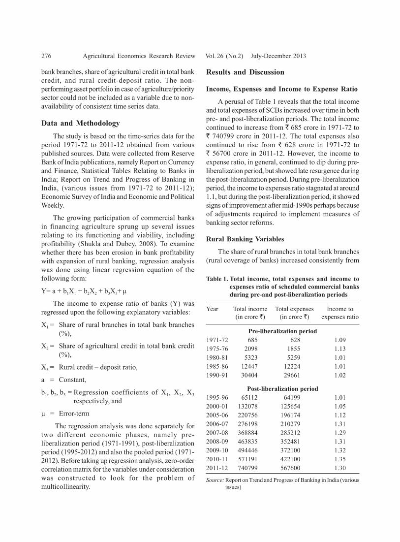
276 Agricultural Economics Research Review Vol. 26 (No.2) July-December 2013
bank branches, share of agricultural credit in total bankcredit, and rural credit-deposit ratio. The non-performing asset portfolio in case of agriculture/prioritysector could not be included as a variable due to non-availability of consistent time series data.
Data and MethodologyThe study is based on the time-series data for the
period 1971-72 to 2011-12 obtained from variouspublished sources. Data were collected from ReserveBank of India publications, namely Report on Currencyand Finance, Statistical Tables Relating to Banks inIndia; Report on Trend and Progress of Banking inIndia, (various issues from 1971-72 to 2011-12);Economic Survey of India and Economic and PoliticalWeekly.
The growing participation of commercial banksin financing agriculture sprung up several issuesrelating to its functioning and viability, includingprofitability (Shukla and Dubey, 2008). To examinewhether there has been erosion in bank profitabilitywith expansion of rural banking, regression analysiswas done using linear regression equation of thefollowing form:
Y= a + b1X1 + b2X2 + b3X3+ μ
The income to expense ratio of banks (Y) wasregressed upon the following explanatory variables:
X1 = Share of rural branches in total bank branches(%),
X2 = Share of agricultural credit in total bank credit(%),
X3 = Rural credit – deposit ratio,
a = Constant,
b1, b2, b3 = Regression coefficients of X1, X2, X3
respectively, and
μ = Error-term
The regression analysis was done separately fortwo different economic phases, namely pre-liberalization period (1971-1991), post-liberalizationperiod (1995-2012) and also the pooled period (1971-2012). Before taking up regression analysis, zero-ordercorrelation matrix for the variables under considerationwas constructed to look for the problem ofmulticollinearity.
Results and Discussion
Income, Expenses and Income to Expense Ratio
A perusal of Table 1 reveals that the total incomeand total expenses of SCBs increased over time in bothpre- and post-liberalization periods. The total incomecontinued to increase from ` 685 crore in 1971-72 to` 740799 crore in 2011-12. The total expenses alsocontinued to rise from ` 628 crore in 1971-72 to` 56700 crore in 2011-12. However, the income toexpense ratio, in general, continued to dip during pre-liberalization period, but showed late resurgence duringthe post-liberalization period. During pre-liberalizationperiod, the income to expenses ratio stagnated at around1.1, but during the post-liberalization period, it showedsigns of improvement after mid-1990s perhaps becauseof adjustments required to implement measures ofbanking sector reforms.
Rural Banking Variables
The share of rural branches in total bank branches(rural coverage of banks) increased consistently from
Table 1. Total income, total expenses and income toexpenses ratio of scheduled commercial banksduring pre-and post-liberalization periods
Year Total income Total expenses Income to(in crore `) (in crore `) expenses ratio
Pre-liberalization period1971-72 685 628 1.091975-76 2098 1855 1.131980-81 5323 5259 1.011985-86 12447 12224 1.011990-91 30404 29661 1.02
Post-liberalization period1995-96 65112 64199 1.012000-01 132078 125654 1.052005-06 220756 196174 1.122006-07 276198 210279 1.312007-08 368884 285212 1.292008-09 463835 352481 1.312009-10 494446 372100 1.322010-11 571191 422100 1.352011-12 740799 567600 1.30
Source: Report on Trend and Progress of Banking in India (variousissues)

Shukla et al. : Factors Affecting Profitability of Commercial Banks 277
noticed in the case of share of agricultural credit intotal bank credit which dipped to 10-13 per cent inpost-liberalization phase after having touched the bestat 18.5 per cent during pre-liberalization phase.However, the share remained below the minimumtarget of 18 per cent, except in the year 1985-86. Asimilar pattern was noticed in the case of rural credit-deposit ratio. This ratio continued to increase duringthe pre-liberalization period and attained the minimumtarget of 60 per cent. However, during post-liberalization period, the C-D ratio fell below the targetlevel of 60 per cent in general, except in the years of2007-08 and 2011-12. It means that of every hundredrupees mobilized as deposits from the rural areas, sixtyrupees were given as agricultural credit in the ruralareas. The share of agricultural credit in total bankcredit continued to increase till mid-1980s, butgenerally decreased thereafter.
Bank Profitability and Rural Banking
The correlation results (Table 3) showed absenceof the problem of multicollinearty. Thus, income toexpenses ratio (Y), as a measure of profitability, wasregressed upon all the three selected variables, X1, X2
and X3 to find as to how the bank profitability getsinfluenced by certain rural banking variables. Thisanalysis was done separately for pre-liberalizationperiod, post-liberalization period and the pooledperiods using the linear regression model.
The regression results (Table 4) showed that duringpre-liberalization period, the share of rural branches(X1), the share of agricultural credit (X2) and the ruralC-D ratio (X3) turned out to be non-significantvariables. In other words, rural banking did not havean adverse influence on the bank profitability duringpre-liberalization period. However, during post-
Table 2. Share of rural branches of banks, share ofagricultural credit in total bank credit and ruralcredit-deposit (C-D) ratio during pre- and post-liberalization periods
Year Share of Share of Ruralrural branches agricultural C-D
of banks credit in total ratio(%) bank credit
(%)
Pre-liberalization period1971-72 36.0 7.2 47.71975-76 36.6 9.2 56.51980-81 51.2 14.2 60.61985-86 55.7 18.5 65.31990-91 56.9 14.2 60.0
Post-liberalization period1995-96 51.2 10.8 47.32000-01 48.3 11.0 39.02005-06 44.5 12.7 56.32006-07 42.1 12.8 60.02007-08 40.6 12.5 60.42008-09 39.6 13.1 57.12009-10 38.2 13.8 59.02010-11 37.4 12.4 59.22011-12 36.9 10.6 72.3
Source: Statistical tables relating to banks in India (various issues)
Table 3. Simple correlation results: 1971-72 to 2011-12
Variable Share of rural Share of agricultural Rural C-D Income tobranches of credit in total bank ratio (X3) expenses ratiobanks (X-1) credit (X2) (Y1)
Share of rural branches of banks (X1) 1 0.612* -0.076 -0.735**Share of agricultural credit in total bank credit (X2) 1 0.462 -0.089Rural C-D ratio (X3) 1 0.389Income to expenses ratio (Y1) 1
Note: **Significant at 10 per cent level*Significant at 5 per cent level
a little more than one-third (36%) in 1971-72 to morethan half (57%) in 1990-91. But, during post-liberalization phase, it started declining and became44 per cent in 2005-06; it further declined to around37 per cent in 2011-12. It was due to the shift in ruralbanking policy from expansion to consolidation bymerging unviable rural branches to improve dwindlingprofitability of banks. An almost similar pattern was

278 Agricultural Economics Research Review Vol. 26 (No.2) July-December 2013
liberalization period the linear regression resultsshowed significant negative effect of share of ruralbranches (X1) on bank profitability. This indicates thatmany of the rural branches were unviable and hencehad to be merged with other branches. Suchconsolidation of branches resulted in a decline in the
share of rural branches in total bank branches as iscorroborated by the data in Table 2. However, theresults for the overall period (1971-72 to 2011-12)indicated that while share of rural branches of banks(X1) had a significant negative effect, the share ofagricultural credit (X2) had a significant positive effecton bank profitability. The rural C-D ratio appeared asa non-significant variable in influencing profitability(Y1) in all the time phases. The total variation explainedin profitability by the three variables together rangedbetween 71 per cent and 91 per cent during differenteconomic phases considered in the study, as indicatedby the adjusted R² estimates.
A perusal at the regression results shown in theTable 4 does not support the view that the increasinginvolvement of banks in the agricultural sector has beenresponsible for the erosion in profitability of banks.The commercial banks are involved not only infinancing agriculture but also in many other sectors ofthe economy such as small, medium and largeindustries, services, exports etc. The commercial bankshave been experiencing high volume of non-performing assets (NPAs) largely in the non-agricultural sector, particularly in industries. Theirexclusion, and a relatively less number of observationsin the time series period, however, make the resultsonly indicative and not conclusive in the present study.
Conclusions and Policy Implications
To turn the negative effect of expansion of ruralbranches into positive effect on profitability, the creditdelivery system will have to be improved by makingcredit delivery timely, adequate, dependable and lesscostly. The credit delivery should be customized byaligning it to the specific content, scale, timing, modeof payment, back up services and cash flow patternsof different sections of rural producers and therebyhelping to reduce non- performing assets of banks.Highly sick rural bank branches which can not bebrought back to normal health may be consolidatedthrough merger with other branches. Similarly, thedeposit mobilization schemes already in operationshould be rationalized and made more popular bymaking them compatible with preferences and cashflow patterns of different sections of rural producers.Thus, the quality of rural banking needs to be upgradedto improve the profitability of banks.
Table 4. Linear regression results on profitability ofbanks as affected by some rural bankingvariables
Independent variable Dependent variablesIncome to expenses
ratio (Y1)
1971-72 to 2011-12 (Total period)Constant (a) 1.165Share of rural branches of banks (X1) -0.0204*
(0.0040)Share of agricultural credit in total 0.0288**bank credit (X2) (0.0125)Rural C-D ratio (X3) 0.00084
(0.0032)Coefficient of multiple determination (R²) 0.788Adjusted R² 0.714
1971-72 to 1990-91 (Pre-liberalization period)Constant (a) 1.052Share of rural branches of banks (X1) 0.0040
(0.0038)Share of agricultural credit in total 0.011bank credit (X2) (0.0147)Rural C-D ratio (X3) 0.0066
(0.0072)Coefficient of multiple determination (R²) 0.923Adjusted R² 0.692
1995-96 to 2011-12 (Post-liberalization period)Constant (a) 1.22Share of rural branches of banks (X1) -0.0213**
(0.0069)Share of agricultural credit in total 0.0209bank credit (X2) (0.0176)Rural C-D ratio (X3) 0.00083
(0.0033)Coefficient of multiple determination (R²) 0.920Adjusted R² 0.872
Notes: Figures within the parentheses indicate standard errors ofregression coefficients,* and ** indicate significance at 0.01 per cent and 0.5 per centlevels, respectively

Shukla et al. : Factors Affecting Profitability of Commercial Banks 279
AcknowledgementsAuthors thank the anonymous referee for his
critical comments and suggestions for betterpresentation of the paper.
ReferencesShukla, A.N. and Dubey, P.P. (2008) Performance of
Commercial Bank Credit to Agriculture in India: An
Empirical Analysis. Ph.D. Thesis, submitted to C.S.J.MUniversity, Kanpur, Uttar Pradesh.
Reserve Bank of India, Report on Trend and Progress ofBanking in India, (various issues from 1971-72 to 2011-12).
Tewari, S.K. (2007) Rapporteur’s report on trends in ruralfinance. Indian Journal of Agricultural Economics,62(3): 551-561.
Received: February, 2013; Accepted August, 2013


Agricultural Economics Research ReviewVol. 26 (No.2) July-December 2013 pp 281-286
Exploring Possibilities of Extending Wheat Cultivation toNewer Areas: A Study on Economic Feasibility of Wheat
Production in Southern Hills Zone of India§
Ajmer Singha*, Rajbir Yadavb and Satyavir Singhc
aCentral Agricultural Research Institute, Port Blair - 744 101, A&N IslandsbDivision of Genetics and Plant Breeding, Indian Agricultural Research Institute, New Delhi - 110 012
cDirectorate of Wheat Research, Karnal -132 001, Haryana
Abstract
The paper has explored the possibilities of expanding cultivation of wheat in the Southern Hills Zone ofIndia by examining the economics of improved wheat varieties demonstrated through front linedemonstrations (FLDs) so as to provide a basis for their adoption and dissemination in farmers’ fields.The average cost of cultivation of improved wheat varieties was higher by about 10 per cent over theirtraditional counterparts due to higher application of inputs and higher price of improved seeds, their unitcost of production was about half of that of the traditional varieties. The economic feasibility of cultivationof wheat in Southern Hills Zone, judged in terms of net returns, has revealed that while cultivationof traditional varieties is not profitable, improved varieties generate significant returns overinvestment.
Key words: Wheat, economic feasibility, southern hills zone
JEL Classification: Q15, O13, R11
IntroductionEver since the introduction of modern varieties in
the mid-1960s, production of wheat in India has grownat an annual rate of 3.9 per cent. The growth occurredboth from area expansion and yield improvements.However, overtime the area expansion has ceased tobe a source of growth and yield growth has decelerated.Between 1996-67 and 1995-96, the area under wheatexpanded at the rate of 1.9 per cent and yield improvedat the rate of 3.3 per cent per annum. But since then,
the growth in its area has decelerated to 0.6 per centand in yield to 0.7 per cent per annum. The states ofUttar Pradesh, Punjab, Haryana, Madhya Pradesh andRajasthan together account for close to 80 per cent ofthe country’s total wheat area and contribute 86 percent to its total production. There is a little scope tobring additional area under wheat in these traditionalwheat-growing states, and the only possibility toincrease wheat production in these states is throughgenetic enhancement.
India has varied climates and there are pockets inthe non-wheat growing states where wheat cultivationcan be promoted, conditional to the availability ofappropriate varieties and cropping practices befittingthe agro-climatic conditions. Jha and Tripathi (2011)having analyzed the effect of climate change on wheatyield, have suggested evaluation of varieties that are
*Author for correspondenceEmail: [email protected]
§The paper has been drawn from the project “Economic analy-sis and impact assessment” which formed a part of largerthematic programme “Technology transfer, refinement andimpact assessment”, DWR/ RP/04/ 11.2 and DWR/ RP/07/12.2.
Research Note

282 Agricultural Economics Research Review Vol. 26 (No.2) July-December 2013
more tolerant to extreme temperatures. The SouthernHills Zone (SHZ) is such a region that has potentialfor introduction of wheat. Almost entire demand forwheat in the southern region of the country is metthrough supplies from the traditional wheat-growingstates or the public distribution system. The locally-produced wheat will work out to be cheaper andaffordable. Under this background, the present studyhas examined the economic possibilities of introducingwheat in the Southern Hills Zone of India.
Biophysical Characteristics of SHZThe SHZ comprises Nigiri hills of Tamil Nadu and
Palni hills of Kerala. During the past two decades, therehas beena shift in the cropping pattern in this Zone,from vegetables towards tea plantation. However, ithas been observed lately that tea plantation is becomingeconomically less remunerative (Shukla and Mishra,2004; Nayeem et al., 2004) and also environmentallyundesirable because of accumulation of toxins in thesoil (Hanchinal et al., 2005). The climate of the SHZis considered suitable for the cultivation of wheat. Theeconomics also appears to favour wheat-vegetablesequence, but is constrained by the problems of rusts,powdery mildew and blight. The lack of availabilityof seeds of improved varieties and irrigation facilitiesare the other constraints in this Zone (DWR, 2004-05;Shukla and Mishra, 2004).
The crop production environment and bio-physicalcharacteristics of Southern Hills Zone are conduciveto growing wheat and support the hypothesis that wheatcan be introduced in this zone and can contribute tonational wheat production significantly if suitablevarieties are identified and production practices arestandardized suited to the agro-climatic conditionsthere. The date of sowing of wheat for this zone hasbeen standardized from November 15 to December 15,whereas harvesting period is 10-20 March. Typically,we can specify as the crop season in this zone from 15Nov to 15 March. During the crop season, themaximum temperature rises up to 25 ºC and minimumtemperature falls to 8ºC which support the crop growthand grain setting. The rains during crop season arebrought by the north-west monsoon and are recordedat 1000-1200 mm. The sunshine for 10 hours duringthe crop season supports crop growth. The zone hasred laterite to clay loam soil type which is again suitablefor wheat cultivation.
MethodologyDuring the crop years 2004-05 to 2009-10, efforts
were made to introduce wheat in this zone throughFront Line Demonstrations (FLDs) by the regionalstation of Directorate of Wheat Research (DWR),Karnal at Wellington in Tamil Nadu. A total of 259experimentations were laid in farmers’ fields indifferent parts of SHZ, mainly in Tamil Nadu. Out ofthese, 46 demonstrations were conducted along withthe checks, whereas in rest of the fields, only latestwheat varieties were planted so as to assess theirsuitability to the socio-economic conditions, economicstrength and acceptability by the farmers. The costsand returns were calculated at the prevailing marketprices. The primary data were recorded on input andoutput levels, socio-economic profile of the farmersand related information. Returns over variable costformed the basis for advocating a particular technologyfor its dissemination and adoption.
The latest technologies including the improvedvarieties are disseminated and up-scaled after these arerefined and adapted to the area-specific peculiaritiesthrough front line demonstrations. Only the progressiveand well-to-do farmers ventured out to produce wheatas was evident from the value of farm inventoriesincluding farm buildings. The participants in the FLDprogramme were included from different farm-categories. Small and medium farmers constituted alarge portion in the sample.
Results and DiscussionThe data showed that wheat crop in this SHZ was
taken with only a limited number of tillage operations.Seed rate used by the farmers was found as per therecommendation, but the number of irrigations andother critical inputs applied in the field were notsufficient to harvest the potential yield. So, the potentialfor wheat production exists in the area, if the level ofmechanization and capital investment requirements ismet appropriately.
Varietal Expanse
The varietal demonstrations were organized in thiszone with the varieties which were suitable to its agro-climatic conditions. In the majority of fields (65 %),the variety HW 3094 developed by IARI, Wellington,was sown under FLDs, though a total of eight varieties

Singh et al. : Exploring Possibilities of Extending Wheat Cultivation to Newer Areas 283
were demonstrated for testing the economic viability(Table 1).
The yield performance showed that varieties HW3070, HD 2833, HW 5018, HW 5001 and COW (W)-1 were superior as they yielded nearly 27-28 q/ha. Thevarieties HW 3094 and HW 2044 were moderateyielders (23-25 q/ha), whereas the varieties HD 2781and HW 1085 gave only 20-21 q/ha. The process ofmineralization is probably not over in this zone andthereby with little increase in the tillage operation withsmall power tillers, the harvest able yield of thesevarieties can be significantly improved. Farmers,generally expressed satisfaction over the performanceof these varieties.
Input Use
It was observed that 40 hours of machine labour,22 hours of bullock labour and 28 person-days ofhuman labour were required per ha for the cultivationof wheat. Land preparation and sowing operations wereperformed manually due to compulsions of resourceendowment, topography and cultural reasons. Ingeneral labour cost was lower on smaller farms weredue to the larger component of women labourers onthese farms who were paid less than their malecounterparts.
Machine labour was used mostly for irrigationpurpose. There was no source of canal irrigation in thestudy area. Mechanical threshers operated by tractorswere used only by large farmers @ 1.20 hours / ha onan average. Land preparation, sowing, harvesting andthreshing consumed more than 80 percent of human
labour requirement. Wage rates were low given thesocio-economic backwardness of the region, but thishas significant implications for future of wheatproduction strategy in the region. Development ofsuitable machineries like power tillers of limited horsepower and minimum cost for land preparation, drillmachines and threshers will be at the core of reducingcost of cultivation in the future. This has also indirectsocio- economic implications with respect to non-farmemployment and farm productivity.
Nutrients Consumption
In the entire sample, N, P, K were applied at therecommended doses in FLDs, whereas in the case ofcheck fields, P and K were applied in less than half ofthe recommended doses (Table 2). FYM was recordedto be added in several fields, but quite low at the rateof 18.2 q/ha. Farmers did show interest in replacinginorganic fertilizers with FYM. On an average, 1604kg of FYM was applied in one hectare every year.
Table 1. Varietal demonstration and performance atfarmers’ fields in SHZ
Varieties Percentage Average yielddemonstrated of farms (q/ha)
HW 3094 46.98 25.23HD 2833 13.02 27.04HW 3070 1.40 28.46HD 2781 2.33 20.78HW 5018 0.47 28.50HW 1085 0.93 21.50HW 2044 2.33 23.28HW 5001 1.86 28.37COW (W) -1 30.70 27.81
Table 2. Nutrients and other critical inputs applied inwheat crop in SHZ
(kg/ha)
Nutrients used FLD Check t- value
Nitrozen (N) 106.77 101.20 1.326*
Phosphorus (P) 47.52 23.48 3.191***
Potash (K) 24.41 12.40 1.861**
Irrigations (No.) 4.52 4.60 -0.576NS
Seed rate 100 100 –No. of ploughings 2.03 2.02 0.252NS
No. of plankings 0.92 0.00 –
Note: ***, ** and * denote significance at 1 per cent, 5 per centand 10 per cent levels, respectively.NS - Not significant
It was found that apart from labour and nutrients,the irrigation, seed and land preparation played a vitalrole in deciding the yield and profitability of wheatcultivation. The number of irrigations was more incontrol fields, but it was not statistically significant.The aberration occurred because some farmers haddemarcated a part of the main field for the checkvarieties and, while irrigating fields, this portion couldnot be spared.
The seed rate was uniform across all farm-categories on FLD as well as control fields. The

284 Agricultural Economics Research Review Vol. 26 (No.2) July-December 2013
planking was used only in FLDs. The number ofploughings was more in small farm-category, but inthe case of irrigations, the situation was the reversedue to resource availability and economic conditionsof large farmers.
Cost and Returns
The operational cost in traditional cultivation wasaround ` 9638/ha, which was less than that of otherregions/zones of the country where the figures varyfrom ̀ 13709/ha in Bihar to ̀ 20508/ha in West Bengal(CACP, 2011).In the case of improved varieties (FLD),it was ` 10703/ha (Table 3) due to higher applicationof inputs and price of improved seeds. The cost ofcultivation including operational cost, interest onworking cost, management charges and risk allowance,was around ` 14391/ha, whereas in the case of checkfields, it was ̀ 12260/ha. The threshing expenses weregenerally higher on smaller farms because proportionof mechanical threshing was higher on larger farmsand it was less in FLD plots as these farmers beingprogressive farmers, had mechanical threshers in higherproportion. It was because of level of mechanizationthat yield levels were higher on large farms.
The unit cost of production was ` 574/q whichwas higher as compared to in NWPZ and other partsof the country largely because of lower yields, whereasin the case of traditional cultivation (check fields), itwas almost double, ` 1131/q. Even this higher cost ofproduction is attractive if the cost of transportation tothis zone is taken into account (Nayeem et al., 2004).The overall profitability depicted by the net returnswas higher at ` 13654/ha in improved varieties thanfrom traditional varieties in check fields, where netreturns were ` 3380/ha. The farmers’ margin arrivedat by adding the imputed value of family labour andmanagement allowance to the net returns was ̀ 16207/hain the case of improved varieties and was –` 917/ha inthe case of traditional wheat cultivation. So, cultivatingwheat using improved wheat production technologiesin this zone has vast economic and social benefits ifcomparative economics vis-à-vis other crops favourwheat cultivation in this zone
A look at the composition of operational costrevealed that expense was highest on fertilizers,followed by seed, land preparation and labour. Theexpenses on harvesting and threshing were almostuniform in all the sample households and expenses on
Table 3. Costs and returns on FLD and check farms(`/ha)
Component Technology situation Difference t- valueFLD Check (%)
Land preparation and sowing 1388 1461 -5.012NS -0.6192Seed 2052 1100 86.57*** 17.8320Fertilizer 2563 1797 42.63*** 5.1810Irrigation 547 832 - 34.18 *** -8.6778Harvesting 902 928 -2.82NS -0.8967Threshing 889 1118 -20.52*** -4.9445Labour charges 2298 2032 13.11*** 4.9991Operational cost 10703 9638 11.05*** 2.6075Cost of cultivation 14391 12260 17.38*** 3.0349Main product (q/ha) 25.89 10.83 139.07*** 17.0574By-product (q/ha) 39.66 25.04 56.85*** 6.5781Cost of production (`/q) 574 1131 -49.25*** -21.9873Gross returns (`/q) 28515 9115 212.74*** 17.9058Net returns (`/q) 13654 -3380 503.96*** 34.7999Returns over variable cost (`/q) 17169 -1098 1663.66*** 16.0948Farmers’ margin (`/q) 16207 -917 1867.39*** 54.6549
Note: ***, ** and * denote significance at 1 per cent, 5 per cent and 10 per cent levels, respectively.NS - Not significant

Singh et al. : Exploring Possibilities of Extending Wheat Cultivation to Newer Areas 285
plant protection were negligible in this zone. The yieldwas quite low at around 25.89 q/ha and thereby returnswere about ` 28515/ha (Table 3), giving a profit of` 13654/ha.
Factors Affecting Wheat Yield
To know the relative effect of the factorsresponsible for variations in wheat yield, the output(Y) was regressed on different inputs like operationalholding (ha), rental value of land (`), present value offarm inventories (`), wheat area sown (ha), ploughings(No.), seed rate (kg/ha), amount of N, P & K (kg/ha)applied, irrigations (No.) and number of person-daysof human labour put to the field to raise the wheat crop.Semi-log linear and log linear functions were fittedand the coefficient values have been presented inTable 4.
In the case of check fields, only P and size of wheatarea planted were found significantly affecting theyields, whereas in FLD plots, operational holding (ha)of the farmer, rental value of land (`/year), value offarm inventories, level of N applied and number ofirrigations were the significant factors affecting theyield levels. The seed rate was uniformly applied inall the FLD fields, whereas labour, P, K, wheat areaand value of farm inventories had no effect on the yields
of improved varieties of wheat. As depicted by thecoefficient of operational holding, rental value of land,irrigation, economic position and resource endowmentof the farmer had a lot to do with the yield levelsobtained in the FLD plots. Non-significance of N incheck fields showed that intensive input-use wasresponsive only to the improved varieties.
Constraints to Wheat Production in SHZ
Wheat being a new crop for this zone, theconstraints to its production have been examined froma different perspective. The constraints in this zonewere quite different in nature than reported from otherparts of the country. The termite infestation wasreported as the most serious problem in this zone,despite the fact that climate of this zone is basicallyhumid and soil is lateritic in structure. The wheatproduction is also hampered by late sowing due toheavy rains and destruction due to wild animals andbirds. Lodging did take place in the case of rains whichwas accompanied by black rust that takes a significanttoll on the wheat productivity in this region. The lackof irrigation facilities is another important constraintand demands serious attention from the planners.Cyprus rotundus (weed) and untimely rains are someof the other constraints but not so serious in nature, asper the reports (Anonymous, 2003-04 to 2009-10a).
Table 4. Factors affecting the yield of wheat in SHZ
Variable FLD plots Check fieldCoefficient Standard error t -value Coefficient Standard error t -value
Operational holding 0.006385 0.00327 1.952844 0.549 0.03645 1.50598Farm inventory -3.1E-06** 1.13E-06 -2.73344 0.0329 0.0361 0.9112Wheat area 0.028066 0.022976 1.221581 0.0991 * 0.0439 2.2567Ploughings -0.11554 0.093671 -1.23346 0.3747 0.2988 1.2536Seed rate 0 0 65535 0 0 65535N 0.006106*** 0.001552 3.934347 0 0 65535P 0.000786 0.001638 0.480012 0.226 * 0.104 2.1750K -0.00246 0.002817 -0.87182 0.0340 0.0334 1.0051Irrigations 0.081491*** 0.017967 4.535591 -0.1203 0.1093 -1.1015Human labour 0.002664 0.003364 0.792106 -0.1153 0.0750 -1.5376(Person-days)R2 0.248 (semi log linear) 0.314 (log linear)
Note:***, **and * denote significance at 1 per cent, 5 per cent and 10 per cent levels, respectively.NS - Non-significant

286 Agricultural Economics Research Review Vol. 26 (No.2) July-December 2013
Conclusions
The study has revealed that SHZ region haspotential to contribute to the total wheat production inthe country and for the economic upliftment of itsresource-poor farmers. The wheat varieties HW 5001,HW 508, COW (W)-1, HD 2833, and HW 3094 havebeen found performing well in this zone. The yieldgain over traditional wheat varieties has been found139 per cent. The unit cost of production per quintalhas been found to be about half under FLDs than oncheck farms. The net returns from improved wheatvarieties are significantly higher, indicating thefeasibility of expanding wheat cultivation in this zone.However, to realize this, some specific measures likeinvestment and encouragement to farm-mechanization,dissemination of labour-saving technologies, anddevelopment and dissemination of suitable varietiesneed to be addressed.
AcknowledgementsThe authors thank the referee for his critical
comments on the paper.
ReferencesAnonymous (2003-04 to 2009-10a) Annual Reports, Social
Science Section, Directorate of Wheat Research,Karnal.
Anonymous (2003-04 to 2009-10b) Annual Reports, WheatSummer Nursery, Indian Agricultural Research Institute,New Delhi.
CACP (2011) Report of the Commission for AgriculturalCosts and Prices – 2010-11, Ministry of Agriculture,Govt of India, New Delhi.
Gondalia, V.K. and Patil, G.N. (2007) An economicevaluation of investment on aonla in Gujarat,Agricultural Economics Research Review, 20(2).
Hanchinal, R.R., Patil, B.N., Kalappanavar, I.K., Math, K.K.,Lohithaswa, H.C., Desai, S.A. and Yenagi Nirmala, B.(2005) 50 Years of Wheat Research in Karnataka,University of Agricultural Sciences, Dharwad.
Lakshmanan, S. (2007) Yield gaps in mulberry sericulturein Karnataka – An econometric analysis, Indian Journalof Agricultural Economics, 62(4).
Jha, Brajesh and Tripathi, A. (2011) Isn’t climate changeaffecting wheat productivity in India, Indian Journalof Agricultural Economics, 66(3).
Nagarajan, S. (1998) Understanding the Issues Involved andSteps Needed to Increase Wheat Yields under Rice/Wheat System — A Case Study of the Karnal Area,Haryana, India, Institute of Plant Diseases,Universityof Bonn, Germany.
Nayeem, K.A., Sivasamy, M., Prabakaran, A.J., Brahma,R.N., Asir, R. and Saikia, A. (2004) Wheat Cultivationin Southern Hills, Areas Adjoining Hills and Plains(Tamil Nadu and Karnataka), IARI Regional Station,Wellington.
Reddy, A.R. and Sen,C. (2004) Technical efficiency in wheatproduction – A socio-economic analysis, AgriculturalEconomics Research Review, 17(2).
Shukla, R.S. and Mishra, P.C. (2004) Influence of ecosystemon components characteristics of wheat genotypes insemi-arid zone. Paper presented at the NationalSymposium on Wheat Improvement for the TropicalAreas organized by IARI, RS, Wellington and TNAU,Coimbatore at TNAU, Coimbatore during 23-25September.
Singh, Ajmer, Singh, Satyavir and Shoran, Jag (2004)Economics of latest wheat production technologies : Azonewise comparison with special reference to tropicalareas. Paper presented at the National Symposium onWheat Improvement for the Tropical Areas, organizedby IARI, RS, Wellington and TNAU, Coimbatore atTNAU, Coimbatore during 23-25 September.
Singh, R.P., Singh, Randhir, Singh, Satyavir, Singh, Ajmer,Mongia, A.D. and Shoran, Jag (2004) DWR ProgressReport, Extension and Economics, Volume 2,AICW&BIP, Directorate of Wheat Research, Karnal.
Singh, Randhir, Singh, Satyavir, Singh, Ajmer, Kumar, Anuj,Singh, R.P., Shoran, Jag and Mishra, B. (2004-05) DWRProgress Report, Information Management andCommunication, AICW&BIP, Directorate of WheatResearch, Karnal.
Revised received: February, 2013; Accepted June, 2013

Agricultural Economics Research ReviewVol. 26 (No.2) July-December 2013 pp 287-292
Production and Marketing of Cumin in Jodhpur Districtof Rajasthan: An Economic Analysis
Vinod Kumar Verma*, Vishnu Shanker Meena, Pradeep Kumar and R.C. KumawatDepartment of Agricultural Economics, S.K.N. College of Agriculture, Jobner-303 329, Rajasthan
Abstract
This study is on the production and marketing of cumin crop in the Jodhpur district of Rajasthan. It isbased on the data collected from 60 cumin–producers in the tehsils of Falodi and Looni during 2009-10.The study has revealed that cumin cultivation in Rajasthan is a profitable enterprise as the returns perrupee invested have been found to be ̀ 1.95 on overall basis, varying from ̀ 1.84 on small farms to ̀ 2.16on large farms. The costs on machine labour (14.4 %) and human labour (13.0 %) have emerged as themajor components in the total operational costs. The cumin–producers have been found to follow twochannels for the marketing of cumin; Channel-I: Farmer → Village trader → Wholesaler→ Retailer; andChannel-II: Farmer→ Wholesaler (Mandi) → Retailer. The marketing cost has been found to be higher inChannel-I due to involvement of more middlemen in the channel. The producer share has been computedas 62.1 per cent in Channel–I and 68.1 per cent in Channel-II. The study has suggested that measuresneed to be adopted to increase access of farmers to market information and they should be motivated tomarket the produce collectively to reduce the cost on transportation.
Key words: Cumin, economic analysis, marketing channel, economic viability, price spread, Rajasthan
JEL Classification: Q13
IntroductionIn India, cumin (Cuminum cyminum) is mainly
cultivated in the states of Gujarat, Rajasthan, UttarPradesh, Madhya Pradesh, Karnataka and Tamil Nadu.Rajasthan with its share of 13.15 per cent stands secondin the total production of cumin in the country. InRajasthan, it is mainly grown in the districts of Jodhpur,Jalore, Barmer, Nagour, Pali, Ajmer, Sirohi, Bhilwaraand Tonk. Information on production, productivity,marketing and income being important to boostproduction of agricultural commodities, particularly onspices, several researchers have studied the economicsof cultivation of ginger, fenugreek, chillies, saffron,etc. (Dodke et al., 2002; Dwivedi and Singh, 2010;Killedar et al., 2002; Rajur et al., 2008; Shah and Zala,
2006; Tripathi et al., 2006). However, such informationseems to be lacking in the case of cumin cultivation inRajasthan. Therefore, the present investigation wastaken up with the following objectives:
• To study the cost of cultivation of cumin crop inRajasthan, and
• To find the marketing behaviour of cumin-growingfarmers and study the costs and returns and pricespread in the marketing of cumin in Rajasthan.
Data and MethodologyJodhpur district having the first place in the
production of cumin in the state was purposely selectedfor the study. Then, two tehsils — Looni and Falodi— of Jodhpur district were selected and from thesetehsils, based on the criteria of maximum productionand sale of cumin, six villages falling under the
*Author for correspondenceEmail: [email protected]
Research Note

288 Agricultural Economics Research Review Vol. 26 (No.2) July-December 2013
command area of Krishi Upaj Mandi Samti, Mandor,were selected. A list of the cumin-growing farmers fromthese villages was prepared and a total of 60 farmers[28 small (< 2 ha), 22 medium (2-4 ha) and 10 large(> 4 ha)] were selected randomly in proportion to theirtotal number in each farm- size group. For study,primary data relating to the agricultural year 2009-10were collected from the selected farmers, wholesalersand retailers through personal interview using a set ofpretested schedules developed specially for thepurpose. The market behaviour of the cumin- growingfarmers and breakup of the consumer’s price, viz.producer’s share in consumer’s rupee, costs ofmarketing and margins of different intermediariesinvolved in cumin marketing channels were workedout.
Results and Discussion
Cost on Cultivation of Cumin Crop
The overall total cost on cultivation (cost c2) ofcumin crop was found to be ̀ 26746/ha, being higheston small (` 27587/ha), followed by medium (` 26257/ha) and large (` 25469/ha) farmers. The total overalloperational cost was found to be ` 18903/ ha, and itwas also highest on small (` 20259/ha), followed bymedium (` 18272/ha), and large (` 16496/ha) farms(Table 1). In the overall operational cost, theexpenditure was highest on machine labour (14.4%),followed by human labour (13.0%) and FYM (9.7%).Thus, machine labour was the main component ofoperational cost and it was found to increase withincrease in farm-size. Another major component of theoperational cost was human labour. It was observedthat the share of human labour was maximum on small(15.0%) farms, followed by medium (12.3%) and large(8.4%) farms.
The higher use of human labour on small andmedium farms was attributed to lesser use of machinelabour in comparison to large farms. The share of plantprotection chemicals in the total cost ranged from 8.47per cent to 9.92 per cent on different farm- size groupswith the average value of 8.94 per cent. The use ofplant protection chemicals was higher on large farms,followed by medium and small farms. The share ofoverhead cost in the total cost was 29.3 per cent onoverall basis and it ranged from 26.6 per cent on smallfarms to 35.2 per cent on large farms, depicting a direct
relationship with farm-size. The rental value of ownedland was the major component of the overhead costs.Its share was 17.4 per cent, 18.2 per cent and 18.9 percent on small, medium and large farms, respectively.Depreciation cost with 7.6 per cent share was thesecond major component of overhead cost and itshowed a positive relationship with the farm-size.
Returns from Cumin Crop
The overall gross income from cumin cultivation,given in Table 2, has been found to be ` 57292/ha inthe study area. This income has depicted a directrelation with farm-size. The average farm businessincome from cumin cultivation was worked out to be` 38758/ha and it has also shown a positive relationwith farm-size. The overall returns over variable costhave been found to be ` 38389/ha. The cost ofproduction was highest on small farms (`5568/q), andminimum on large farms (`4748/q), depicting aninverse relationship with farm-size.
Costs, Margins and Price Spread in Marketing ofCumin Crop
It was found that farmers adopt following twochannels for marketing of cumin:
Channel-I : Farmer → Village trader → Wholesaler→ Retailer
Channel-II : Farmer → Wholesaler (Mandi) →Retailer
The marketing costs in both the channels wereworked out and are presented below.
Channel-I
The marketing costs incurred in Channel-I havebeen depicted in Table 3. A perusal at Table 3 revealedthat the total cost in marketing of cumin at village levelwas `1043 / q. Among the three intermediaries in thischannel, the retailer bore the maximum marketing cost(` 655/q) due to VAT and the wholesaler had to pay` 329/q as the Mandi fee. It was noted that VAT aloneaccounted for the maximum share (60.8%) in the totalmarketing costs, followed by Mandi fee (16.6%) andcommission charges (10.36 %). Transportation chargesamounted to 5.5 per cent of the total marketing costsin Channel-I. The stakeholder-wise break up indicatedthat the highest cost was borne by the retailer (62.8%),

Verma et al. : Production and Marketing of Cumin in Jodhpur District of Rajasthan 289
Table 1. Operational and overhead costs in the cultivation of cumin crop on sample farms in Jodhpur district ofRajasthan: 2009-10
(` /ha)
Particulars Farm-size groupsSmall (< 2ha) Medium (2-4 ha) Large (> 4ha) Overall
(A) Operational costsBullock labour 2274 998 382 1491
(8.24) (3.80) (1.50) (5.58)Machine labour 3304 4283 4420 3849
(11.98) (16.32) (17.36) (14.4)Seed 2107 2218 2414 2199
(7.64) (8.45) (9.48) (8.22)FYM 3373 2144 1366 2588
(12.23) (8.17) (5.36) (9.7)Fertilizers 373 489 606 454
(1.35) (1.86) (2.38) (1.70)Plant protection chemicals 2337 2401 2527 2392
(8.47) (9.14) (9.92) (8.94)Irrigation charges 1747 1973 2162 1899
(6.34) (7.51) (8.49) (7.10)Interest on working capital 590 532 480 550
(2.14) (2.03) (1.89) (2.06)Human labour 4150 3230 2134 3477
(15.04) (12.30) (8.38) (13.0)Sub-total of operational costs 20259 18272 16496 18903
(73.44) (69.59) (64.77) (70.67)
(B) Overhead costsDepreciation 1626 2132 2997 2040
(5.89) (8.12) (11.77) (7.63)Rental value of owned land 4800 4800 4800 4800
(17.40) (18.20) (18.85) (17.95)Land revenue 20 20 20 20
(0.07) (0.08) (0.08) (0.07)Interest on fixed capital 881 1032 1155 982
(3.20) (3.94) (4.54) (3.68)Sub-total of fixed costs 7328 7985 8973 7843
(26.56) (30.42) (35.23) (29.33)Total cost (A+B) 27587 26257 25469 26746
Note: The figures within the parentheses are per cent of total cost
followed by wholesaler (31.5%) and village trader(5.3% ). The farmer- producer had to bear 0.4 per centof the total marketing cost in Channel-I.
Channel-II
The marketing cost incurred in marketing of cuminin Channel-II, depicted in Table 4, was found to be
` 1022/q. Among the two intermediaries figured inChannel-II, the retailer bore the maximum marketingcost (` 654/q) due to the payment of VAT and thewholesaler had to pay ̀ 329/q as the Mandi fee. In thetotal marketing cost in Channel-II, the VAT accountedfor the highest share (62.0%), followed by Mandi fee(16.9%) and commission charges (10.6%).

290 Agricultural Economics Research Review Vol. 26 (No.2) July-December 2013
Table 3. Marketing cost of cumin in Channel-I in Jodhpur district of Rajasthan: 2009-10(`/q)
Particulars Cost borne by ConsumerProducer Village trader Wholesaler Retailer cost
Transportation - 39 9 9 57(70.9) (2.73) (1.37) (5.46)
Gunny bag 4 5 6 6 21(100) (9.0) (1.82) (0.92) (2.01)
VAT - - - 634 634(96.79) (60.79)
Mandi fee - - 173 - 173(52.58) (16.59)
Commission - - 108 - 108(32.83) (10.35)
Brokerage - - 27 - 27(8.21) (2.59)
Loading + unloading - 11 6 6 23sieving, weighing, etc. (20) (1.8) (0.92) (2.21)Total 4 55 329 655 1043
(0.4) (5.3) (31.5) (62.80) (100)
Assumptions: (1) VAT will be borne by the retailer. (2) Commodity is transferred from producer to retailer
Transportation charges amounted to ` 47/q (4.6%) inChannel-II. The stakeholder-wise break up indicatedthat the highest cost was borne by the retailer (63.9%),followed by wholesaler (32.2%) and producer-farmer(3.8%).
Price Spread
Price spread in cumin in both the marketingchannels is discussed below:
Channel–I
The details of price spread in marketing of cuminin Channel-I are given in Table 5. It shows that thecumin-farmer got ` 9845 /q (62.1%) out of theconsumer price of ` 15854/q. The marketing costsincurred by the producer, village trader, wholesaler andretailer were 0.02 per cent, 0.35 per cent, 2.07 per centand 4.13 per cent, respectively of the price paid by theconsumer. These together accounted for 6.57 per cent
Table 2. Returns from cultivation of cumin crop in Rajasthan: 2009-10 (in `/ha)
Particulars Farm- size groupsSmall Medium Large Overall
Gross income 55884 57627 60498 57292Farm business income 37377 39199 41658 38758Returns over variable cost 35625 39355 44002 38389Family labour income 31815 32287 35486 32602Net income 25538 28743 32487 27871Returns per rupee 1.84 1.99 2.16 1.95Cost of production (`/q) 5568 5154 4748 5198

Verma et al. : Production and Marketing of Cumin in Jodhpur District of Rajasthan 291
of the consumer’s price. In the total marketing marginof ` 4967/q, the share was highest of retailer (` 2459/q, 15.5%), followed by wholesaler (`1573/q, 9.9%)and village trader (`941/q, 5.9%).
Channel-II
The details of price spread in marketing of cuminin Channel-II in Rajasthan are given in Table 6. It showsthat the cumin-farmer got `10807 /q out of theconsumer price of ̀ 15854/q, (68.16%). The marketingcosts incurred by the producer, wholesaler and retailerwere worked out to be 0.24 per cent, 2.07 per cent and
Table 4. Marketing cost of cumin in Channel-II in Jodhpur district of Rajasthan: 2009-10(`/q)
Particulars Cost borne by ConsumerProducer Wholesaler Retailers cost
Transportation 29 9 9 47(74.36) (2.73) (1.37) (4.60)
Gunny bag 4 6 6 16(10.26) (1.82) (0.92) (1.56)
VAT - - 634 634(96.94) (62.03)
Mandi fee - 173 - 173(52.58) (16.93)
Commission - 108 - 108(32.83) (10.57)
Brokerage - 27 - 27(8.21) (2.64)
Loading + unloading, sieving, weighing, etc. 6 6 5 17(15.38) (1.8) (0.76) (1.66)
Total 39 329 654 1022(3.81) (32.19) (64.0) (100)
Assumptions: (1) VAT will be borne by the retailer. (2) Commodity is transferred from producer to retailer
Table 6. Price spread in marketing of cumin in Channel–IIin Rajasthan: 2009-10
Particulars ` /q Share in consumerrupee (%)
Producer’s share 10807 68.16Costs incurred by
(a) Producer 39 0.24(b) Wholesaler 329 2.07(c) Retailer 654 4.13
Total cost 1022 6.45Margin earned by
Wholesaler 1573 9.92Retailer 2452 15.47
Total margin 4025 25.39Consumer’s price 15854 100.00
Table 5. Price spread in marketing of cumin in Channel–Iin Rajasthan: 2009-10
Particulars ` /q Share in consumer’srupee (%)
Producer’s share 9845 62.10
Cost incurred by(a) Producer 4 0.02(b) Village trader 55 0.35(c) Wholesaler 329 2.07(d) Retailer 655 4.13
Total cost 1043 6.57
Margin earned by(a) Village trader 941 5.94(b) Wholesaler 1573 9.92(c) Retailer 2453 15.47
Total margin 4967 31.33Consumer’s price 15854 100.00

292 Agricultural Economics Research Review Vol. 26 (No.2) July-December 2013
4.13 per cent, respectively of the price paid by theconsumer. The total marketing costs and marketingmargins accounted for 6.45 per cent and 25.39 per cent,respectively in the consumer’s price. The marketingmargin was higher of retailer (`2452/q, 15.47%) thanof wholesaler (` 1573/q, 9.92%).
ConclusionsThe study has revealed that cumin cultivation is a
profitable enterprise in the Jodhpur district ofRajasthan. The net income on overall basis has foundto be ̀ 27871/q, ranging from ̀ 25538/q on small farmsto ` 32487/q on large farms. The marketing cost hasbeen found to be higher by ` 21/q when cumin wassold through Channel-I due to involvement of moremiddlemen in this channel. The study on price spreadin marketing of cumin in Channel has shows asignificant difference in the margins of intermediaries.Of the consumer rupee, the village trader received 5.94per cent share, wholesaler received 9.92 per cent, andretailer got 15.47 per cent share. Among all thefunctionaries, the margin of retailers was higher dueto the sale of cumin in piecemeal at high prices to theconsumers. The producer’s share in consumer’s rupeein the sale of cumin directly in the regulated market ofMandor was 68.2 per cent as compared to 62.1 percent in sale at village level. For marketing of cumin,the channels followed are: Channel-I: Farmer→ Villagetrader → Wholesaler→ Retailer, and Channel-II:Farmer→ Wholesaler (Mandi) → Retailer.
RecommendationsThe study has made following recommendations:
(i) The farmers should be educated to sell theirproduce in the regulated markets which fetchhigher returns as compared to village levelmarketing.
(ii) The farmers should be motivated to transport theirproduce collectively to lower the cost ontransportation and hence on marketing,particularly by the small farmers.
AcknowledgementsThe authors thank the referee for his helpful
comments on the earlier draft of this paper whichhelped in improving its presentation also.
ReferencesDodke, L.B., Kalamkar, S.S., Shende, N.V. and Deoghare,
B.L. (2002) Economics of production and marketingof fenugreek. Indian Journal of Agricultural Marketing,16 (2): 69-74.
Dwivedi, Sudhaker and Singh, Tarunvir (2010) An analyticaleconomics of saffron cultivation in Jammu andKashmir. Journal of Hill Agriculture, 1 (2): 168-171.
Killedar, N.S., Lahor, N.S., Babar, V.S. and Ingavale, M.T.(2002) Economics of production and marketing ofginger in Satara district of western Maharashtra. IndianJournal of Agricultural Marketing, 16 (2): 76-77.
Rajur, B.C., Patel, B.L. and Basavaraj (2008) Economicsof chilli production in Karnataka. Karnataka Journalof Agricultural Science, 21 (2): 237-240.
Shah, S.P. and Zala, Y.C. (2006) Cost-benefit analysis ofginger cultivation in middle Gujarat. AgriculturalEconomics Research Review, 19 (Conference issue):206.
Singh, R.P. and Toppo, Anupama (2010) Economics ofproduction and marketing of tomato in Kanke block ofRanchi district. Indian Journal of AgriculturalMarketing, 24 (2): 1-16.
Tripathi, A.K., Mandal, Subhasis, Datta, K.K. and Verma,M.R. (2006) Study on marketing of ginger in Ri- Bhoidistrict of Meghalaya. Indian Journal of Marketing, 20(2): 106-115.
Revised received: August, 2013; Accepted: October, 2013

Agricultural Economics Research ReviewVol. 26 (No.2) July-December 2013 pp 293-297
Post-harvest Losses in Wheat Crop in Punjab: Past and Present§
D.K. Grover* and J.M. SinghAgro Economic Research Centre, Punjab Agricultural University, Ludhiana – 141 004, Punjab
Abstract
The crop losses during the process of harvesting, threshing, transportation and storage of foodgrains arequite significant. The present study has estimated the extent of losses occurring during post- harvestphase of wheat crop based on the experience of 120 wheat-growing farmers of various farm-size categoriesfrom Ludhiana and Ferozepur districts of Punjab. The study has observed that harvesting losses weremore for the late harvested crop due to shattering of the grains, while losses during transportation, handlingand rodents attack in the case of stored grains have been found insignificant. In totality, the post-harvestlosses have been worked out to be 1.84 per cent currently. Earlier studies had estimated such losses to be9.3 per cent during 1971and 3.71-3.85 per cent in 1992. Thus, better post-harvest management has resultedin minimizing post-harvest losses. The study has suggested timely harvesting of wheat crop andorganization of training programmes for control of rodents / fungus/pests attack to further curtail thelosses at field level.
Key words: Post-harvest losses, wheat crop, post-harvest management, Punjab
JEL Classification: Q11, Q16
IntroductionThe production and availability of foodgrains are
sometimes mistakenly used as synonyms. To estimatethe food supplies correctly, the losses during and afterharvest in terms of storage, transportation andmarketing, etc. need to be studied scientifically. Theproduction in agriculture is exposed to naturalenvironment, but post-production operations play animportant role in providing stability in the food supplychain. Losses in food crops occur during harvesting,threshing, drying, storage, transportation, processingand marketing. In the field and during storage, theproducts are threatened by insects, rodents, birds and
other pests. Moreover, the product may be spoiled byinfection from fungi, yeasts or bacteria. Food grainstocks suffer both qualitative and quantitative losseswhile in storage. To minimize the losses during storageit is important to know the optimum environmentconditions for the storage of product, as well as theconditions under which insects/pests damage theproduce. Birewar (1977) has stressed the need of equalimportance to quality and quantity of the grainsproduced and the losses during post-harvest operationswere estimated to be of the order of 10 per cent inIndia. Gill and Singh (1986) have reported the totallosses in foodgrains, including the losses at thethreshing floor, as 9.33 per cent in Punjab. Accordingto a FAO study, about 70 per cent of the farm produceis stored by the farmers for household consumption,seed, feed and other purposes in India. Farmers storegrain in bulk using different types of storage structuresmade from locally available materials. For the betterstorage it is necessary to clean and dry the grain toincrease its life during storage. In addition, storage
*Author for correspondenceEmail: [email protected]
§This research article is drawn from research report entitled“Assessment of Pre and Post Harvest Losses of MajorFoodgrains in Punjab”, carried out by Agro EconomicResearch Centre, Ludhiana, and sponsored by Ministry ofAgriculture, Government of India, New Delhi
Research Note

294 Agricultural Economics Research Review Vol. 26 (No.2) July-December 2013
structure, design and its construction also play a vitalrole in reducing or increasing the losses during storage.With the scientifically constructed storage, it is alsoessential that the grain being stored is also of goodquality. Generally, harvesting is done at high moisturecontent and, therefore, before storing the same, it isnecessary to obtain the desired moisture to obtain safepost-storage grain.
Basavaraja et al. (2007) have estimated grain lossesduring wheat harvesting in Karnataka state as 0.36 kgper quintal. These losses were mainly due to sheddingof grains. The amount of loss depended on the cropstage and time of harvesting. The losses duringcleaning/winnowing operation were estimated to be0.14 kg per quintal. The average losses have beenworked out to be 0.45 quintal per hectare. Singh et al.(1992) have estimated the post-harvest losses in wheatcrop in Punjab to be 1.49-1.55 per cent duringharvesting (sickle-harvested) and 1.57-1.60 per cent(combine-harvested). The wheat loss during threshingwas 1.42-1.45 per cent and during marketing was 0.80per cent.
During the past two decades, there have beenseveral developments in farming- related operations.These include increased use of farm-mechanization,reduction in harvesting period, increased roadconnectivity, better road network, increasedtransportation facilities, superior packaging material,etc. These coupled with longer experience of foodgrainshandling of farmers must have affected the post-harvestmanagement of foodgrains. Thus, there was an urgentneed to assess the post-harvest losses in foodgrainsunder the changed scenario and get fresh estimates oftheir net availability. Therefore, the present study wasconducted in Punjab with the following specificobjectives:
• To estimate the post-harvest losses in wheat cropduring various post-harvest handling operations,and
• To study the impact of better management andother developments on post-harvest losses ofwheat crop.
Materials and MethodsThe study is based on the farm level data collected
from two major wheat-growing districts, namely
Ludhiana and Ferozepur, of Punjab. The post-harvestlosses during different farming operations,transportation and storage were quantified based onthe estimates provided by the farmers. To collect theprimary data, a sample survey was conducted in theselected districts during rabi 2010-11 (November toMay). Ludhiana district represented the central plainregion, while Ferozepur district represented the south–western region of the state. From each district, twovillages — one nearby the market/mandi centre andthe other far off from the market centre — were selectedand from each village 30 wheat- growing farmers wereselected randomly, constituting the total sample of 120farmers. The farm-size-wise there were 22 marginal(< 2.50 acres), 24 small (2.51-5.00 acres), 24 medium(5.01-10.00 acres) and 50 large (> 10.00 acres) farmersin the sample. In addition to the primary data, districtoffice of the Department of Agriculture as well asexperts at Punjab Agricultural University were alsoconsulted to find wheat loss estimates during post-harvest operations. Simple statistical tools were usedto interpret the survey results.
Results and DiscussionThe results have been discussed under the
following sub-heads: (i) Socio-economic status ofrespondents, (ii) Post-harvest losses, and (iii) Impactof better management and infrastructural facilities.
Socio-economic Status of Respondents
The socio-economic characteristics of the samplehouseholds revealed that the average number of incomeearners were two in all the farm-size categories, exceptin large category, where there were three earners. Thefarmers interviewed were mostly household-head andthe average age of 71-79 per cent respondents wasabove 40 years, and of 12-26 per cent was between 25and 40 years. Most of the sample farmers were educatedthough educational level varied. The annual householdincome varied from `1.65 lakh to `12.60 lakh, beinglowest on marginal and highest on large farmcategories. The share of owned land was more on allthe farm-size categories as compared to leased-in orleased-out land. The net operated area on overall basiswas 11.4 acres, it being 2.2 acres on marginal, 3.9 acreson small, 8.0 acres on medium, and 20.7 acres on largefarmers. The farms of all categories were irrigated andthe cropping intensity was nearly 200 per cent. Paddy

Grover and Singh : Post-harvest Losses in Wheat Crop in Punjab 295
was the major kharif crop (occupying nearly 40% ofgross cropped area), followed by basmati (6.1%) andfodder crops (3.7%). Wheat was the major rabi crop(occupying 46.9 per cent of gross cropped area),followed by rabi fodder with 2.7 per cent area. Theentire area sown under various kharif, rabi, summerand perennial crops was under HYV seeds, as revealedby the sample households.
Post-harvest Losses in Wheat Crop
This section presents the assessment of productionlosses during harvesting, threshing/ winnowing,transportation, handling, storage along with,quantitative assessment of storage and pest controlmeasures adopted by the selected households.
Production Loss during Harvest
The production losses during different stages ofwheat harvesting have been depicted in Table 1. Aperusal of Table 1 shows that the average wheat areaharvested per household was highest (8.85 acres)during the mid stage of harvesting, followed by latestage (1.62 acres) and early stage (0.21 acres). In termsof percentage, it was 82.9 per cent in mid season, 15.1per cent in late and 2.0 per cent in early season. Of thetotal 10.68 acres area harvested per household, 2.14acres (20.0%) was harvested manually and 8.54 acres
(80.0%) mechanically. The area mechanicallyharvested in terms of stages of harvesting was highestin mid (79.1%), followed by late (18.4%) and early(2.5%) stages. The area manually harvested in the midstage was 98.1 per cent and just 1.9 per cent washarvested during late season. The ranking of loss duringdifferent stages of crop harvest was reported to be lowby 2 per cent households during early stage, 86 percent during mid stage and 12 per cent during late stageof harvesting. The quantity of wheat lost per acre was20.4 kg during early, 26.7 kg in the mid and 47.2 kg inthe late harvesting stages of wheat crop. Therefore,wheat loss at different stages was 1.1 per cent in early,1.4 per cent in mid and 2.5 per cent in late harvesting.The higher wheat loss in late harvesting was due toshattering of grains in the fields. The lower loss in theearly harvesting was due to the negligible (2.0%) areabeing harvested during this stage.
Production Loss during Threshing and Winnowing
It was reported by 35 per cent of the sample farmersthat presently threshing was being done mechanicallyusing a thresher and winnowing was not requiredseparately due to the facility of fan in the threshingoperation itself. The average loss was 3.95 kg/acrewhich came out to be just 0.20 kg/quintal on the samplefarms.
Table 1. Quantity lost at different harvesting stages of wheat crop
Particulars Stages of wheat harvest OverallEarly Mid Late
Area harvested per household (acres) 0.21 8.85 1.62 10.68Percentage area harvested 2.0 82.9 15.1 100.0Area manually harvested (acres) - 2.10 0.04 2.14
(20.0)*Percentage area manually harvested - 98.1 1.9 100.00Area mechanically harvested (acres) 0.21 6.75 1.58 8.54
(80.0)*Percentage area mechanically harvested 2.5 79.1 18.4 100.0Quantity lost during harvest
kg/acre 20.4 26.7 47.2 28.7kg/quintal 1.1 1.4 2.5 1.5% of harvest amount 1.1 1.4 2.5 1.5
Note: Figures within the parentheses show percentage of total area harvested

296 Agricultural Economics Research Review Vol. 26 (No.2) July-December 2013
Production Loss during Transportation andHandling
It was found that tractor- trolley was the only modebeing used by the sample farmers to transport theirproduce to the market. The average quantity transportedper household was 183.5 quintals, and the averagedistance covered was 4.1 km with transportation costof ` 3.60/quintal.
The average loss in wheat during transportationwas found to be 0.06 kg/q, which was just 0.0003 percent of the total quantity of wheat transported.Similarly, the average loss in wheat due to handling atdifferent stages was calculated as 0.20 kg/q which wasmerely 0.001 per cent of the handled quantity. Thus,loss during transportation and handling was negligiblein wheat crop. The transportation losses were low dueto the use of tractor-trolley and better management ofwheat grains with special care of putting gunny as wellas plastic covers, beneath as well as on the sides of thetrolley before filling it with the produce to be sold inthe market.
Production Loss during Storage
Although, there are several modes of wheatstorage, the one being adopted by the samplerespondents was of steel drum and the average wheatstored was 19.5 quintals per household. It was observedthat for storage of wheat proper scientific method wasbeing followed by the respondents of using properly-dried steel drums for filling of wheat grains, applyingproper fumigation to the produce and making thecontainer airtight by applying wet soil on its openings.All the households reported drying of wheat grainsbefore storage. The stored produce was graduallywithdrawn as per household requirement and, therefore,was stored for the whole year. The rank of losses was‘low’ as reported by all the sample households. Theaverage wheat quantity lost during storage was reportedto be 0.012 kg/q due to rodents and 0.008 kg/q due tofungus infection. The storage cost has been workedout to be ` 3.35 per quintal of stored quantity.
Total Post-harvest Losses in Wheat
The total post-harvest losses in wheat, depicted inTable 2, reveal that the highest loss was duringharvesting of wheat crop. It was estimated to be 1.52kg per quintal. The losses during threshing,
transportation and storage were found very small; thesewere 0.04 kg/q, 0.06 kg/q and 0.02 kg/q, respectively.The wheat loss during loading/ unloading was alsofound to be small (0.2 kg/q). In total, the post-harvestlosses in wheat crop worked out to be 1.84 kg/q or35.14 kg/acre. Thus, major grain loss (82.60%) wasincurred during harvesting of wheat crop while duringother post- harvest operations, the losses were meagre.
Conclusions and Policy ImplicationsThe study has brought out that post-harvest losses
in wheat crop have declined with the passage of time.These losses were estimated as 10 per cent in India byBirewar (1977). On the other hand, Gill and Singh(1986) reported these losses as 9.30 per cent in Punjab.Later on, Singh et al. (1992) have estimated the post-harvest losses in wheat to be 3.71-3.85 per cent whichincluded losses during harvesting (sickle and combine),threshing and marketing operations. The presentinvestigation has estimated the total post-harvest lossesin wheat to be 1.84 per cent in Punjab. These are quitesmall and can be attributed to the mechanical harvestingof a significant area under this crop. It has also beenobserved that the losses during wheat harvesting arehigh in case of late harvesting of the crop due toshattering of grains. Hence, farmers should be advisedto undertake timely harvesting of wheat crop tominimize harvesting losses. There is also a need toimpart training to the farmers on scientific handlingand better management of grains, particularly duringstorage to minimize the post-harvest losses.
Due to adoption of latest farm technologies withemphasis on mechanization of various farm operations,Punjab farmers have minimized post-harvest losses attheir farms. The judicious use of farm resources and
Table 2. The post-harvest losses in wheat crop
Loss in different operations Amount lost(kg/q)
Harvest 1.52Threshing 0.04Transport 0.06Handling including loading/uploading 0.20Storage 0.02Total post-harvest losses (kg/q) 1.84Total post-harvest losses (kg/acre) 35.14

Grover and Singh : Post-harvest Losses in Wheat Crop in Punjab 297
better post-harvest management by the farmers haveplayed a significant role in curtailing the grain lossesin wheat crop.
ReferencesBasavaraja, H., Mahajanashetti, S.B. and Udagatti, Naveen
C. (2007) Economic analysis of post-harvest losses infood grains in india: A case study of Karnataka.Agricultural Economics Research Review, 20(1): 117-26.
Birewar, B.R. (1977) Post- harvest operations, Productivity,18(2): 227-40.
Gill, K.S. and Singh, R. (1986) Marketing and Handling ofWheat and Paddy in the State of Punjab, Departmentof Processing, College of Agricultural Engineering,Punjab Agricultural University, Ludhiana. pp.16-26.
FAO (Food and Agriculture Organization), Research andDevelopment Issues in Grain Post-harvest Problemsin Asia; www.fao.org/wairdocs/x5002e/X5002e02.htm
Singh, G., Singh, J., Thapar, V. K., Sehgal, V. K. and Paul,S. (1992) Post-production losses of wheat at farm levelin Punjab, Bulletin of Grain Technology, 30: 20-27.
Revised received: June 2013; Accepted September, 2013


Abstracts of M.Sc. Theses
R.B. Godambe (2013): Economics of Productionand Disposal of Okra (Abelmoschus esculentus (L.)Moench) in Thane District, Department ofAgricultural Economics, College of Agriculture, Dr.Balasaheb Sawant Konkan Krishi Vidyapeeth, Dapoli-415 712, Maharashtra
Major advisor: Dr S.R. Torane
This study has been conducted in the Thane districtof Maharashtra with a sample of 135 okra growersusing the data pertaining to the agricultural year 2011-12. The study has revealed that the average size oflandholding was 2.8 ha, of which net cultivated areawas 2.5 ha. At overall level, the total cost of cultivationwas ` 191660/ha, gross returns were ` 488637/ha andnet profit was ̀ 296977/ha. The input-output ratio was1:2.55, indicating that okra is a highly profitableenterprise. Seed, fertilizer, plant protection and humanlabour have been found to have statistically significantand positive influence on yield. However, they werebeing excessively used and decreasing returns to scalewere observed.
The three marketing channels operating in studyarea were: (1) Producer → consumers, (2) Producer→ retailers → consumers, and (3) Producer →commission agent-cum wholesalers → retailers →consumers. The highest quantity of okra was soldthrough channel-III. However, the producer’s share inconsumer’s rupee was highest (98.26%) in channel-I.Non-availability of certified seed, high cost of plantprotection chemicals, high transportation cost, widefluctuations in price and high commission charges havebeen identified as the major problems being faced bythe okra growers.
The problems reported by the vegetable traderswere unstable prices, lack of market information, andlack of sanitary facilities in the market yard. The studyhas concluded that okra being a profitable crop, higherresources need be allocated for development of high-yielding seeds and capacity building of farmers inhaving a better access to market information.
B.C. Karbhari (2013): Economics of Production andDisposal of Arecanut in Raigad District, Departmentof Agricultural Economics, College of Agriculture, Dr.Balasaheb Sawant Konkan Krishi Vidyapeeth, Dapoli-415 712, Maharashtra
Major advisor: Dr V.A. Thorat
The economics of production and disposal ofarecanut has been studied in the Raigad district ofMaharashtra by selecting total 155 gardens. The datapertained to agricultural year 2011-12. The study hasrevealed that the per hectare cost of establishment forarecanut garden was ` 182463 of which maximum(63.1%) was incurred on human labour, followed byFYM (16.0%) and planting material (12.6%). The costof maintenance for arecanut garden was worked out tobe ` 261762/ha, of which highest (31.8%) was therental value of land, followed by hired male labour(18.7%) and amortization value (13.9%). The overallgross returns were ` 499000/ha, of which maximumreturns (47.6%) were obtained from arecanut, followedby coconut (23.55%) and black pepper (9.2%).
The net returns were highest from arecanut +coconut + black pepper cropping system (` 189098),followed by (` 189033) arecanut + coconut + blackpepper + cinnamon cropping system. The study hasrevealed that values for NPV, BCR (at 15% discountrate) and IRR were ` 22348, 1.05 and 16.67,respectively with payback period of 6 years. Acrossthe different cropping systems, NPV (` 58200), BCR(1.10) (at 15% discount rate) and IRR (17.49%) werehighest in arecanut + coconut + black pepper croppingsystem with payback period of 6 years. To studyresource-use efficiency in arecanut, the Cobb-Douglasstype production function was fitted. It was found thatamong different inputs, the use of human labour (bothmale and female) was in excess and use of fertilizers,manures, and plant protection chemicals was belowthe optimum level.
The study has revealed that at overall level, thetotal production of arecanut was 1319 kg, and almostall the produce was sold in the market. The marketedshares of other commodities were also high. Thesewere: coconut 91.0 per cent, black pepper 90.1 per cent;nutmeg 98.8 per cent; cinnamon 90.8 per cent; banana94.0 per cent and pineapple 85.6 per cent.
Agricultural Economics Research ReviewVol. 26 (No.2) July-December 2013 pp 299-301

300 Agricultural Economics Research Review Vol. 26 (No.2) July-December 2013
D.A. Killedar (2013): Study of Co-operative CreditSocieties in Sindhudurg District, Department ofAgricultural Economics, College of Agriculture, Dr.Balasaheb Sawant Konkan Krishi Vidyapeeth, Dapoli-415 712, Maharashtra
Major advisor : Dr H.K. Patil
This study has been undertaken with a randomsample of 144 borrowers (72 defaulters and 72 non-defaulters) from 36 co-operative credit societies in theSindhudurg district of Maharashtra. The total averagefarm business income was ` 1,21,015 in the non-defaulters group and ` 21,125 in the defaulters group.The average income from other sources was ` 45,781in non-defaulters group and ` 25,390 in defaultersgroup.
The average amount borrowed was ` 98,960 bynon-defaulters group and ̀ 16,732 in defaulters group.The share of short-term borrowing was more in boththe groups, it being 84.4 per cent in non-defaulters and82.2 per cent in defaulters groups. In non-defaultersgroup, the highest share of short-term credit wascontributed for fruit crops (76.6%) and in defaultersgroup, it was contributed for rice (88.8%).
The non-defaulters group had utilized 83.4 per centof its short-term borrowings for productive purposesand 16.6 per cent was diverted towards unproductiveuse. The defaulters group had utilized a lower share(57.3%) of their total short-term borrowings forproductive purposes. In the case of medium-term credit,the non-defaulters group utilized 76.4 per cent of theirborrowings for productive purposes and 23.6 per centwas diverted to the unproductive uses. The defaultergroup utilized only 17.0 per cent of total borrowingfor productive uses and 83.0 per cent was used forunproductive purposes.
The results of logistic regression model haverevealed that the variables education and proportionof credit utilized for productive purpose were positivelyrelated with non-defaulters. As the level of educationand the proportion of credit used for productive purposeincreased, the probability to be a non-defaulter alsoincreased.
P.N. Kumbhar (2013): Marketing of Mango inSouth Konkan Region of Maharashtra – AnEconomic Analysis, Department of AgriculturalEconomics, College of Agriculture, Dr. BalasahebSawant Konkan Krishi Vidyapeeth, Dapoli-415 712,Maharashtra
Major advisor: Dr A.C. Deorukhakar
This study on the marketing of mango in southKonkan region of Maharashtra is based on theinformation collected from 120 mango growers for theyear 2011-12. On overall basis, the average productionwas found to be 26.34 q/ha and the average number oftrees per hectare was 104. The per farm area of orchardwas 1.56 ha and per farm average number of trees was163, with average production of 36.8 quintals.
At overall level, the total quantity of mangoes soldwas 36.13 quintals, of which 6.95 per cent was soldon-farm and 4.76 per cent in the local market. Thequantity sold in distant market was 88.29 per cent, ofwhich 78.19 per cent was sold in the Mumbai marketand remaining in the Pune and Kolhapur markets.
The study has observed that mango is marketedthrough five channels: (I) Producer → consumer (directsale), (II) Producer → wholesaler/commission agent→ retailer → consumer, (III) Producer → pre-harvestcontractor → wholesaler/commission agent → retailer– consumer, (IV) Producer → co-operative society →consumer, (V) Producer → fruit merchant → hawker→ consumer. The per quintal cost of marketing washighest in channel III (` 2116), followed by channel II(` 1906), channel IV (` 917), channel V (` 886) andchannel I (` 358).
The price spread of mango fruits showed that theproducer’s share in consumer’s price was highest(95.0%) in channel I and lowest (31.8%) in channelIII. The gross margin of commission agents andretailers in channel II was 8.75 per cent and 22.95 percent, respectively. The gross margin of pre-harvestcontractors in channel III was 36.48 per cent, whereas,the gross margin of co-operative society in channel IVwas 15.49 per cent.
The gross market margin has been found highestin channel III (68.2%), and minimum in channel I(5.0%). The marketing efficiency has been observedhighest in channel I and lowest in channel III. Formarketing of mango, channel I has been found to bemost efficient, but most of the cultivators sell theirproduce through commission agents.

Agricultural Economics Research Review Vol. 26 (No.2) July-December 2013 301
R.D. Mhaske (2013): Economics of Production andDisposal of Turmeric in Sindhudurg District (M.S.),Department of Agricultural Economics, College ofAgriculture, Dr. Balasaheb Sawant Konkan KrishiVidyapeeth, Dapoli-415 712, Maharashtra
Major advisor : Dr V.G. Naik
The economics of production and disposal ofturmeric has been studied with a sample of 100cultivators drawn from Sawantwadi, Dodamarg, Kudaland Vaibhavwadi tahsils in Sindhudurg district ofMaharashtra. The data pertained to the agricultural year2011-2012. In input-use, the proportion was more offamily labour days than of hired labour days in all sizegroups of turmeric farms. About 40 per cent of the totalhuman labour (243 person-days) was used forharvesting, nursery bed preparation and sowingoperations. The cost of cultivation of turmeric workedout to be ` 1,79,063/ha and net returns were ` 51,450/ha. The benefit-cost ratio worked out to be 1.29.
To estimate the contribution of explanatoryvariables on turmeric yield, Cobb-Douglas productionfunction (log linear form) was fitted. The coefficientsof determination (R2) indicated 84.7 per cent variationin turmeric production. The coefficients of seed, humanlabour, fertilizers and manures were statisticallysignificant and the ratio of MVP to factor cost for seed,human labour, fertilizers and plant protection was lessthan one, indicating excess utilization of theseresources.
The per farm total production was 228.2 kg ofwhich 29.8 per cent was retained for seed purpose and70.2 per cent was available for disposal. The quantityof processed turmeric rhizomes was 78.3 kg, of which96.3 per cent was sold, remaining 2.7 per cent wasused for family consumption and 1.0 per cent was givento the relatives.
The major constraints being faced by the turmericcultivators were fluctuations in market price (62.0%),incidence of pests and diseases (39.0%), non-availability of labour on time (32.0%), difficulties insecuring seed of improved varieties (30.0%) andstorage problems (20.0%).
V.V. Vibhute (2013): Economics of Production andDisposal of Kokum in South Konkan Region,Department of Agricultural Economics, College ofAgriculture, Dr. Balasaheb Sawant Konkan KrishiVidyapeeth, Dapoli-415 712, Maharashtra
Major advisor: Dr S.S. Wadkar
This study has been undertaken in the southKonkan region of Maharashtra with a sample of 120kokum cultivars (40 having grafted origin kokumorchard and 80 having seed origin kokum orchards).The information was collected for the agricultural year2011-12. The study has revealed that the growth ratein area and production of kokum has increasedsignificantly over the period for both Ratnagiri andSindhudurg districts. The cost of establishment ofkokum orchard for the initial five years has been foundto be higher (` 64038/ha) in grafted kokum orchardthan in seed origin kokum orchard (` 32977/ha). Thecost of production was also higher in grafted kokumorchard (` 37884/ha) than in seed origin kokum orchard(` 25572/ha).
The per hectare kokum production was 60.8quintals and 61.7 quintals in grafted and seed originkokum orchards, respectively. The kokum cultivationhas been found to be a profitable enterprise at all thelevels of cost and in both types of kokum orchards.The benefit-cost ratio was 1.20 and 1.81 in graftedkokum orchards and seed origin kokum orchards,respectively. The cost of production has been found tobe higher in grafted kokum orchard (` 623/q) than inseed origin kokum orchard (` 415/q).
All financial feasibility tests in kokum plantationhave been found positive for grafted as well as seedorigin kokum orchards, indicating that kokumcultivation was an economically-feasible enterprise.


Abstracts of Ph.D. Theses
(Ms) A.V. Nikam (2013): Economics of OilseedCrops in Maharashtra, Department of AgriculturalEconomics, MPKV, Rahuri – 413 722, Dist.Ahmednagar, Maharashtra
Major Advisor: Dr B.V. Pagire
This study has analyzed the past performance,present scenario and future prospects for oilseedsproduction in Maharashtra based on the districtwisetime-series data for the period 1960-61 to 2009-10.The study has also projected supply-demand estimatesof oilseeds in Maharashtra by 2019 and 2029. The studyhas revealed that the area under oilseeds in Maharashtrahas increased from 17.56 lakh ha to 39.87 ha duringthis period. Across different regions of the state, areaunder oilseeds has increased in Marathwada andVidarbha regions, and declined in Konkan and westernMaharashtra regions. During this 50-year period, theproduction of total oilseeds in the state has increasedby 305 per cent and productivity by 78.6 per cent.
Among different oilseeds, the area under kharifgroundnut, safflower and sunflower has decreased by74.8 per cent, 39.7 per cent and 28.7 per cent,respectively, and increased under soybean by 5560.8per cent. The production of kharif groundnut in thestate has decreased by 52.3 per cent and of soybean,safflower and sunflower has increased by 102.5 percent, 72.6 per cent and 9.7 per cent, respectively. Inthe state, for the entire period, the area and productionof soybean have increased significantly at the rate of31 per cent and 33 per cent per annum, respectively,while the productivity has shown a growth rate of 1.73per cent per annum. The growth rate of area, productionand productivity of total oilseeds were 1.7, 3.8 and2.0, respectively for the entire period. The growth ratesof area, production and productivity of total oilseedswere positive but non-significant for the pre-TMOperiod, and were positive and significant for the post-TMO period.
The estimated supply of oilseeds in Maharashtrawould be 50.2 lakh tonnes by 2019 and 56.8 lakh tonnesduring 2029 by taking the productivity constant; itwould be 61.3 lakh tonnes and 82.9 lakh tonnes by2019 and 2029, respectively on considering the
productivity growth to be 2.0 per cent per annum. Asagainst this, the demand for oilseeds would be 28.2-29.5 lakh tonnes for rural population and 49.8 to 52.0lakh tonnes for urban population by 2019 underdifferent situations. The gaps in availability anddemand for oilseeds in Maharashtra would be in therange of 28.2-30.8 lakh tonnes by 2019 and 110.1-122.6lakh tonnes by 2029 assuming the constantproductivity. By assuming increasing productivity @2.0 per cent per annum, the gaps in availability anddemand for oilseeds would be in the range 17.2-19.7lakh tonnes by 2019 and 83.9-96.4 lakh tonnes by 2029.Therefore, efforts need to be made to increase the areaunder oilseeds by making irrigation available andincreasing its potential. A positive price policy isrequired to increase the area and/or to bringimprovement in productivity. The supply-demand gapfor oilseeds can be bridged by increasing the adoptionof improved technology through strengthening of theTMO.
Huma Sehar (2013): Productivity and SustainabilityMeasurements of Cropping System in Jammu,Department of Agricultural Economics, Sher-e-Kashmir University of Agricultural Sciences andTechnology – Jammu
Major Advisor: Dr Jyoti Kachroo
This study has been carried out on the basissecondary data on area, production and productivityof various crops grown in the Jammu region. The datafor calculating total factor productivity andsustainability were collected from various annualreports of Farming System Research Centre (FSRC),SKUAST-J and for estimating supply response werecollected from various organizations and departments.The study has revealed a significant increase in areairrigated by wells, from 2.35 per cent in 1981 to 6.16per cent in 2010; however, area irrigated by canals hasbeen found to be highest (84.16%). In the Jammuregion, rice, maize and wheat crops had togetheroccupied more than 80 per cent of the gross croppedarea during the past three decades. The results ofexpansion effect have shown that the area had expandedto its limit and there exists the substitution effect now
Agricultural Economics Research ReviewVol. 26 (No.2) July-December 2013 pp 303-304

304 Agricultural Economics Research Review Vol. 26 (No.2) July-December 2013
which ultimately leads to crop diversification. Yieldinstability was the major source of variability whichincreased in rice, maize and wheat and decreased inpulses over the years.
For the entire study period (1986-87 to 2010-11),the OLS and MLE coefficients for human labour, seeds,phosphorus, irrigation and miscellaneous charges havebeen found positive, and for herbicide, urea, FYM andmachine labour have been found negative. Theestimated yield gap I has been recorded to be 26.19per cent and 26.47 per cent for rice and wheat,respectively. The total yield gap has been recorded tobe 66.12 per cent in rice and 57.42 per cent in wheat.
The supply elasticity with respect to own priceelasticity for rice has been found to be 0.070 in short-run and 0.065 in long-run, while in the case of wheat,the elasticities were 0.311 and 0.846 in the short-runand long-run, respectively. The estimated own priceelasticity of maize has been found as -0.426 in the short-run and -0.385 in long-run.
The study has concluded that substitution effect ishigher than expansion effect. The total factorproductivity has been found to be less than one formost of the period. The own price elasticity has beenfound positive for all the crops studied, except formaize.

Book Review
Agricultural Growth and Productivity inMaharashtra — Trends and Determinants, byS.S. Kalamkar, Allied Publishers Pvt Ltd, New Delhi.2011, pp. 218 + xviii. ISBN: 978-81-8424-692-6, Price` 500/-
Agricultural growth plays an important role inachieving national goals which include providing foodand nutritional security, reducing rural poverty,supplying raw materials to major industries and earningforeign exchange, among others. A number of analystshave examined the trends in agricultural productivityand the determinants of stagnation in productivity ofimportant crops. The book under review mainly coversdistrict-wise growth and stagnation in production ofimportant crops in the state of Maharashtra. It analysesthe regional variations in Maharashtra at district level,identifies the determinants of these variations andsuggests appropriate interventions to address theproblem of stagnation.
The book is organised under six chapters. Chapter-I introduces the topic and analyses the growth in area,production and productivity of major crops/crop groupsin India and Maharashtra’s contribution thereto. Therecent developments in agriculture of Maharashtra arediscussed in Chapter-II. Chapter-III covers themeasurement of growth and stagnation in cropproductivity, while Chapter-IV analyses the trends andpatterns in production and productivity in Maharashtraat the district level. The determinants of productivitystagnation of major agricultural crops in Maharashtraare discussed in Chapter-V. Finally, Chapter-VIsummarises the findings and draws conclusions forpolicy advocacy.
The book is mainly based on the secondary datacollected for the period 1960-61 to 2004-05 fromvarious published sources, mainly from Maharashtra.The book first provides an overview of the recentagricultural developments in Maharashtra. Though
performance of agriculture has improved during thepast fifty years, its progress has not been sustained andshows wide fluctuations. The recent suicides of farmersin the Vidarbha and Marathwada regions have onceagain highlighted the regional disparity in agriculturaldevelopment in Maharashtra. Due to low irrigationfacilities (hardly 18%), not only low-value crops arebeing cultivated predominantly in the state, but theproductivity of most of the crops is also very lowcompared to the national average.
The cropping pattern in Maharashtra has thoughshown a shifting trend in favour of high-value crops inrecent years, this shift is not impressive vis-a-vis at thenational level. For instance, in 2004-05 coarse cerealswhich accounted for only about 15 per cent of the grosscropped area (GCA) at all-India level, accounted forover 30 per cent of GCA in Maharashtra, which ranksfirst in area and production of coarse cereals, mainlyjowar and bajra. Similarly, the share of area underpulses in GCA has declined to about 1.31 per cent atall-India level in 2004-05, but the same has increasedby 2.31 per cent in Maharashtra, which is the secondlargest producer of pulses after Madhya Pradesh,wherein tur and gram are two important pulse cropsgrown in most of the districts in the state. Area underoilseeds, especially soybean and cotton is also higherin Maharashtra (a total of 17.98% of GCA in 2004-05)as compared to all-India average (15.41%). Apart fromthese crops, sugarcane is another important crop of thestate, which accounted for 22 per cent of the totalnational production in 2006-07, but the productivityhas remained almost constant during the past few years,due to sugarcane mono-cropping, which has evendeteriorated the soil fertility. Strict rules need to beenacted to discourage the cultivation of sugarcaneunder flood irrigation method by introducingvolumetric pricing for canal water, at least in the areaswhere productivity is declining.
Agricultural Economics Research ReviewVol. 26 (No.2) July-December 2013 pp 305-306

306 Agricultural Economics Research Review Vol. 26 (No.2) July-December 2013
One of the significant changes that have taken placein the cropping pattern of Maharashtra recently is thedevelopment of horticultural crops. Area under fruitand vegetable crops has increased by about 6-timesover the past 40 years. The major factors limiting thegrowth of horticultural sector in Maharashtra have beenlimited crop diversification in non-traditional areas,deceleration in area and productivity of certain cropsand poor post harvesting infrastructural facilities. Asfuture growth of agriculture in the state is heavilydependent on the performance of horticultural sector,it is essential to examine the growth rate of certainhorticultural crops. Introduction of drought-resistantHYVs, promoting balanced use of fertilizers and well-designed location-specific policies or programmes likewatershed development can help increase theproductivity of crops appreciably.
The book further elaborates on the rate and growthof agricultural inputs. The pattern of land use has beenfairly stable at the state level since 1961, with marginaldownward change in the share of forest area or increasein the proportion of land under non-agricultural use.Further, there has been a decrease in the irrigationintensity of the state due to low space growth in grossirrigated area as compared to the net irrigated area.The area under HYVs in the state has declined in fewdistricts. The district-wise growth rate of creditdisbursement by PACS has indicated a significantincrease in credit disbursement to agriculture and alliedsector in all the districts of the state. Along with this,the state has recorded an increase in the number ofplant protection equipments and tractors. The keydriver of economy, viz. annual growth rate ofelectricity-use in agriculture, has shown that despitelimited availability, consumption of electricity foragriculture in the state has significantly increased. Theuse of one of the important yield-increasing inputs,namely fertilizer, is considerably lower in Maharashtra
than all-Indian average. Poor irrigation facilitiescoupled with cultivation of low value crops are themain reasons for low use of fertilizers.
The book reveals based on the total factorproductivity (TFP) growth rate analysis that the numberof regulated markets and annual rainfall are the mostimportant sources of growth of agriculture inMaharashtra. The effect of research, literacy andrainfall in TFP has been found negative. Therefore,there is a need to target public investment in theresearch field. The significant deceleration in TFPgrowth during the later period in respect of major cropshas serious implications for the agriculturaldevelopment. This food-deficit state may witness afurther decline in food production. Therefore, there isan urgent need to increase TFP growth in the majorcrops to make their cultivation profitable and toincrease crop diversification and optimal use of landand other resources.
The main strength of this book is the extensivedata collected by the author and other contributors forvarious crops grown in different districts ofMaharashtra. The book has adequately focussed onvarious critical issues concerning agricultural growthin Maharashtra, which provide many policyimplications that need to be taken up by theGovernment of Maharashtra to maintain sustainablegrowth in production. The findings and policyimplications of the study are expected to be useful tothe policymakers for formulating region-specificpolicies focussing on agricultural development inMaharashtra. The book provides an interesting readingfor students, research managers and developmentalagencies.
Prof. V.R. KiresurDepartment of Agricultural Economics
University of Agricultural SciencesDharwad, Karnataka

Agricultural Economics Research ReviewVol. 26 (No.2) July-December 2013 pp 307-308
Agricultural Economics Research ReviewGuidelines for Submission of Papers/Abstracts
1. The journal publishes research articles, reviewarticles, research notes and communications inbasic and applied research on economic aspectsof agriculture and rural development.Comprehensive review articles in the area ofagricultural economics (including livestock,horticulture and fisheries), conference/symposiaproceedings and book reviews are also publishedin the Journal. To encourage the young researchers,recent abstracts of M.Sc. and Ph.D. theses inagricultural economics are also published.
2. The journal is managed by the eminent economistsunder the domain of Agricultural EconomicsResearch Association (India). The authorssubmitting papers to Agricultural EconomicsResearch Review should be members of thisAssociation.
3. Two copies of manuscript typed in double spaceshould be sent to
The Managing EditorAgricultural Economics Research ReviewF-4, A BlockNational Agricultural Science Centre ComplexDev Prakash Shastri MargPusa, New Delhi - 110 012
and a soft copy to [email protected]. All articles must include anabstract in about 100-150 words.
4. Authors should include the complete source ofresearch article, like project, along with sponsor,M.Sc./Ph.D. thesis, etc. They should mention thetitle of the Project/Thesis also.
5. The length of papers should not be more than 20(double space) typed pages, including tables,diagrams and appendices.
6. Abstracts of recent M.Sc. theses should not exceedone typed page and those of Ph.D. theses, twotyped pages. The authors must mention at the topof the abstracts the degree for which the thesis
was submitted and the year of award, like M.Sc.(2008), Ph.D. (2008). The name of ‘major advisor’should also be included.
7. Name(s) and affiliation(s) of the author(s) with e-mail address(es) should be provided on a separatepage along with the title of the article.
8. Only essential mathematical notations may beused. All statistical formulae should be neatlytyped. Footnotes should be numberedconsecutively in plain arabic superscripts.
9. References: Only cited works should be includedin reference list. The citation of references shouldbe in the following order: author(s) name(s); year;title of article; name of journal; volume; number;and pages. Please follow the style of citations asin the latest issue of this journal. Papers notsubmitted in the standard format, as suggestedabove will not be considered for publication.
The reference list should be alphabetized and notnumbered. To avoid ambiguity, the title of journalshould be given in full.
The following examples, as typical enteries,provide guidance for enteries in the reference list.
Research Paper: Rosegrant, M.W. and Pingali,P.I. (1994) Policy and technology for riceproductivity growth in Asia. Journal ofInternational Development, 6(6): 6656-88.
Book: Rosegrant, M.W. and Hazell, P.B.R. (2000)Transforming Asian Economy: The UnfinishedRevolution. Oxford University Press, Hong Kong.
Chapter in a Book or Paper in a publishedproceedings: Kumar, P. (2001) Agriculturalperformance and productivity. In: IndianAgricultural Policy at the Crosswords, Eds: S.S.Acharya and D.P. Chaudhri. Rawat Publication,New Delhi, pp. 353-476.

308 Agricultural Economics Research Review Vol. 26 (No.2) July-December 2013
Paper in a Conference/Symposium: Kapoor,B.C. (2000) Managing in the face of not-so-developed and organized environment. In:Proceedings of National Symposium onManagement and Development, held at Instituteof Public Administration, Jaipur, 23-25 July.
Thesis: Behera, Sumanta (2004) Impact ofTechnological Change and Economics of CocoonProduction in Mandya District of Andhra Pradesh,MSc (Seri Technol) Thesis, submitted toUniversity of Mysore.
Units: Use SI units; a few examples are givenbelow:
Hectare ha Milligram mgRupees ` Million hectares MhaLitre L Tonne tMillilitre mL Million tonnes MtGram g Metre mKilogram kg Centimetre cm
Please note that no full stop is used after theabbreviation of units.
10. Papers submitted for publication should beexclusively written for this journal and should nothave been published or sent for publicationelsewhere.
11. The journal Agricultural Economics ResearchReview is available on-line, please contact at thefollowing addresses for on-line services:(i) Divan Enterprises
B-9, Basement, Block-ANaraina Vihar, New Delhi 110 028, Indiahttp:// www.indianjournals.com
(ii) AgEcon SearchWaite LibraryDepartment of Applied EconomicsUniversity of Minnesota1994 Buford AveSt. Paul MN 55108-6040, USAhttp:// www.agecon search
12. Membership Tariffs/Subscription to AgriculturalEconomics Research Review* (Effective fromJanuary, 2010)
Particulars Print copy E- Print +publication Online
(E-publication)
NationalInstitutional ` 2000/- ` 2000/- ` 3000/-Membership
Individual ` 500/- ` 500/- ` 750/-Membership
Student ` 400/- ` 400/- ` 600/-Membership
Life ` 4000/- ` 4000/- ` 4000/-Membership
OverseasInstitutional US $ 150 US $ 150 US $ 300Membership
Individual US $ 75 US $ 75 US $ 75Membership
Life US $ 500 US $ 500 US $ 500Membership
* Payment should be made through Demand Draft ormulticity cheque payable to Treasurer, AgriculturalEconomics Research Association at New Delhi.
The annual subscription includes two regular issues of thejournal and a Conference Number.
Address for correspondence:Secretary/TreasurerAgricultural Economics Research AssociationF-4, A BlockNational Agricultural Science Centre ComplexDev Prakash Shastri Marg, PusaNew Delhi - 110 012Email: [email protected]: www.aeraindia.in
Correspondence may preferably be donethrough E-mail.

AGRICULTURAL ECONOMICS RESEARCH ASSOCIATION (INDIA)
OFFICE BEARERS
President : Dr. P.G. Chengappa, National Professor, Institute for Social and EconomicChange, Bangalore – 560 072 (Karnataka)
Conference President : Dr. V.P.S. Arora, Vice Chancellor, Supertech University, Rudrapur (Uttarakhand) (2013)
Vice Presidents : Dr. K.C. Hiremath, Former Professor, UAS, Dharwad, XI Cross Road, NirmalNagar, Dharwad – 580 003 (Karnataka)
Dr. P. Kumar, Former Professor, Division of Agricultural Economics, IndianAgricultural Research Institute, New Delhi – 110 012
Secretary : Dr. Suresh Pal, Head, Division of Agricultural Economics, Indian AgriculturalResearch Institute, New Delhi – 110 012
Treasurer : Dr. V.C. Mathur, Professor, Division of Agricultural Economics, Indian AgriculturalResearch Institute, New Delhi – 110 012
Joint Secretaries : Dr. Anjani Kumar, Principal Scientist, National Centre for Agricultural Economicsand Policy Research, Pusa, New Delhi – 110 012
Dr. M.H. Wani, Divison of Agricultural Economics and Marketing, Sher-e-KashmirUniversity of Agricultural Science and Technology-K, Shalimar Campus, Srinagar– 191 121 (Jammu & Kashmir)
Members : Dr. Anil Kumar Dixit, Senior Scientist (Agricultural Economics), Central Instituteof Post Harvest Engineering & Technology, Ludhiana – 141 004 (Punjab)
Dr. (Ms) Nikita Gopal, Scientist, Central Institute of Fisheries Technology, P.O.Matsyapuri, Cochin – 682 029 (Kerala)
Dr. Manjeet Kaur, Farm Economist, Department of Economics and Sociology,Punjab Agricultural University, Ludhiana – 141 004 (Punjab)
Dr. V.R. Kiresur, Professor of Agricultural Economics, Department of AgriculturalEconomics, University of Agricultural Sciences, Dharwad – 580 005 (Karnataka)
Dr. Naveen P. Singh, Principal Scientist, National Institute of Abiotic StressManagement, Baramati – 413 115 (Maharashtra)
Dr. R.K.P. Singh, Former Professor, RAU, 101/A, Shivam Heritage, AshianaRoad, Patna – 800 001 (Bihar)
Dr. Smita Sirohi, Principal Scientist (Dairy Econ.), National Dairy ResearchInstitute, Karnal – 132 001 (Haryana)
Dr. K.C. Talukdar, Professor, Department of Agricultural Economics, AssamAgricultural University, Jorhat – 785 013 (Assam)

Agricultural Economics Research Review
ISSN 0971-3441Online ISSN 0974-0279
Agricultural Economics Research Association (India)
Regd. No. F2 (A/67)/89
Agricultural Economics Research Association (India), a registered society which came into being in 1987, has on date more than 745 life members, 110 ordinary members, more than 115 institutional members and 25 honorary life members from India and abroad. The mandate of the Association is to promote the study of agricultural economics in particular and socio-economic problems in general. The Association has been regularly publishing a six-monthly research Journal “Agricultural Economics Research Review” since 1988. Besides refereed research articles, comprehensive review articles in the area of agricultural economics (including horticulture and fisheries), conference/symposia proceedings and book reviews are also published in the Journal. To encourage the young researchers, abstracts of M.Sc. and Ph.D. theses in agricultural economics are also published in the Journal. The Association has been successfully organizing national conferences regularly on topical policy issues, the proceedings of which have been published. The Association undertakes sponsored research studies. Over the years, the Association has attained a wide visibility and professional credibility. The official journal of the Association, namely, Agricultural Economics Research Review has been highly rated by National Academy of Agricultural Science, New Delhi.
Address for Correspondence:SecretaryAgricultural Economics Research Association (India)F-4, A Block, National Agricultural Science Centre (NASC) ComplexDev Prakash Shastri Marg, PusaNew Delhi 110 012, India
Email: [email protected]: www.aeraindia.in
Agricultural Economics Research Association (India)
About the Association
Printed at Cambridge Printing Works, B-85, Naraina Industrial Area, Phase-II, New Delhi - 110 028.
July-December2013Volume 26Number 2
V.P.S. ARORA: Agricultural Policies in India: Retrospect and Prospect
SURESH C. BABU , P.K. JOSHI, CLAIRE J. GLENDENNING, KWADWO ASENSO-OKYERE AND RASHEED SULAIMAN V.: The State of Agricultural Extension Reforms in India: Strategic Priorities and Policy Options
RASHMI AGRAWAL, S.K. NANDA, D. RAMA RAO AND B.V.L.N. RAO: Integrated Approach to Human Resource Forecasting: An Exercise in Agricultural Sector
LIJO THOMAS, GIRISH KUMAR JHA AND SURESH PAL: External Market Linkages and Instability in Indian Edible Oil Economy: Implications for Self-sufficiency Policy in Edible Oils
ELUMALAI KANNAN: Does Decentralization Improve Agricultural Services Delivery? — Evidence from Karnataka
ANJANI KUMAR, SHINOJ PARAPPURATHU AND P.K. JOSHI: Structural Transformation in Dairy Sector of India
HARI KRISHNA SHRESTHA, HIRA KAJI MANANDHAR AND PUNYA PRASAD REGMI: Investment in Wheat Research in Nepal – An Empirical Analysis
GIRISH K. JHA AND KANCHAN SINHA: Agricultural Price Forecasting Using Neural Network Model: An Innovative Information Delivery System
AKHTER ALI: Farmers’ Willingness to Pay for Index Based Crop Insurance in Pakistan: A Case Study on Food and Cash Crops of Rain-fed Areas
RANJIT KUMAR PAUL, SANJEEV PANWAR, SUSHEEL KUMAR SARKAR, ANIL KUMAR, K.N. SINGH, SAMIR FAROOQI AND VIPIN KUMAR CHOUDHARY: Modelling and Forecasting of Meat Exports from India
PAVITHRA S. AND KAMAL VATTA: Role of Non-Farm Sector in Sustaining Rural Livelihoods in Punjab
Y. LATIKA DEVI, JASDEV SINGH, KAMAL VATTA AND SANJAY KUMAR: Dynamics of Labour Demand and its Determinants in Punjab Agriculture
A.N. SHUKLA, S.K. TEWARI AND P.P. DUBEY: Factors Affecting Profitability of Commercial Banks: A Rural Perspective
AJMER SINGH, RAJBIR YADAV AND SATYAVIR SINGH: Exploring Possibilities of Extending Wheat Cultivation to Newer Areas: A Study on Economic Feasibility of Wheat Production in Southern Hills Zone of India
VINOD KUMAR VERMA, VISHNU SHANKER MEENA, PRADEEP KUMAR AND R.C. KUMAWAT: Production and Marketing of Cumin in Jodhpur District of Rajasthan: An Economic Analysis
D.K. GROVER AND J.M. SINGH: Post-harvest Losses in Wheat Crop in Punjab: Past and Present
AG
RIC
ULT
UR
AL
EC
ON
OM
ICS
RE
SE
AR
CH
RE
VIE
W Vo
l. 26 (2) July-D
ecemb
er 2013
se eR a s rcci h m Ao sn so oc ciE a l ta ior nut l (Iu nci dr iag )A