Takustr. 714195 Berlin

GermanyZuse Institute Berlin

BERNHARD KAPLAN, JENS BUCHMANN, STEFFENPROHASKA, AND JAN LAUFER

Monte-Carlo-based inversion schemefor 3D quantitative photoacoustic

tomography

ZIB Report 17-04 (March 2017)

Zuse Institute BerlinTakustr. 714195 BerlinGermany

Telephone: +49 30-84185-0Telefax: +49 30-84185-125

E-mail: bibliothek@zib.deURL: http://www.zib.de

ZIB-Report (Print) ISSN 1438-0064ZIB-Report (Internet) ISSN 2192-7782

Monte-Carlo-based inversion scheme for 3D quantitativephotoacoustic tomography

Bernhard A. Kaplana, Jens Buchmannb, Steffen Prohaskaa, and Jan Lauferc

aVisual Data Analysis, Zuse Institute Berlin, Takustr. 7, 14195 Berlin, GermanybInstitute of Optics and Atomic Physics, Technical University Berlin, Straße des 17. Juni 135,

10623 Berlin, GermanycInstitut fur Physik, Martin-Luther-Universitat Halle-Wittenberg, Halle (Saale), Germany

ABSTRACT

The goal of quantitative photoacoustic tomography (qPAT) is to recover maps of the chromophore distribu-tions from multiwavelength images of the initial pressure. Model-based inversions that incorporate the physicalprocesses underlying the photoacoustic (PA) signal generation represent a promising approach. Monte-Carlomodels of the light transport are computationally expensive, but provide accurate fluence distributions predic-tions, especially in the ballistic and quasi-ballistic regimes. Here, we focus on the inverse problem of 3D qPATof blood oxygenation and investigate the application of the Monte-Carlo method in a model-based inversionscheme. A forward model of the light transport based on the MCX simulator and acoustic propagation modeledby the k-Wave toolbox was used to generate a PA image data set acquired in a tissue phantom over a planardetection geometry. The combination of the optical and acoustic models is shown to account for limited-viewartifacts. In addition, the errors in the fluence due to, for example, partial volume artifacts and absorbersimmediately adjacent to the region of interest are investigated. To accomplish large-scale inversions in 3D, thenumber of degrees of freedom is reduced by applying image segmentation to the initial pressure distribution toextract a limited number of regions with homogeneous optical parameters. The absorber concentration in thetissue phantom was estimated using a coordinate descent parameter search based on the comparison betweenmeasured and modeled PA spectra. The estimated relative concentrations using this approach lie within 5 %compared to the known concentrations. Finally, we discuss the feasibility of this approach to recover the bloodoxygenation from experimental data.

Keywords: quantitative photoacoustic tomography, model-based inversion, oxygen saturation, chromophoreconcentration, photoacoustic imaging, Monte Carlo methods for light transport, boundary conditions, coordinatesearch

1. INTRODUCTION

Photoacoustic tomography (PAT) is a hybrid imaging method combining optical excitation of tissues andacoustic detection of the induced ultrasound waves.1 The main advantages of PAT are based on its high contrastdue to the spectral specificity of tissues, the low-scattering nature of ultrasonic waves, the large penetrationdepth of light in the near infrared regime causing a high depth-to-resolution ratio, and its ability to noninvasivelyprovide in-vivo images at multiple spatial scales.2

In quantitative photoacoustic tomography (qPAT), the goal is to accurately determine the absolute concen-tration of light absorbing chromophores. One of the main contrast agents in PAT is blood in form of oxygenatedhemoglobin and deoxygenated hemoglobin. The ratio of oxygenated hemoglobin and total hemoglobin sO2

provides physiological information about the metabolism and changes in the vasculature, which makes it animportant marker for a variety of pathologies characterized by metabolic or structural changes in the vascula-ture,3 e.g. tracking of tumor growth and therapy in-vivo.4 Model-based inversion schemes have been shown tobe a promising approach for the recovery of chromophore concentrations from PA images quantitatively.5,6

Further author information: (Send correspondence to B.A.K., J.L.)B.A.K.: E-mail: kaplan@zib.de, Telephone: +49 30 841 85-339J.L.: E-mail: jan.laufer@physik.uni-halle.de, Telephone: +49 345 55 25 400

Copyright 2017 Society of Photo Optical Instrumentation Engineers. One print or electronic copy may be made forpersonal use only. Systematic electronic or print reproduction and distribution, duplication of any material in this

paper for a fee or for commercial purposes, or modification of the content of the paper are prohibited.Citation: Bernhard A. Kaplan ; Jens Buchmann ; Steffen Prohaska ; Jan Laufer; Monte-Carlo-based inversion scheme

for 3D quantitative photoacoustic tomography. Proc. SPIE 10064, Photons Plus Ultrasound: Imaging and Sensing2017, 100645J (March 23, 2017); doi:10.1117/12.2251945

http://proceedings.spiedigitallibrary.org/proceeding.aspx?articleid=2614022

In order to determine sO2 from PA images, multiwavelength measurements and some form of spectralunmixing, i.e. the recovery of the relative contribution of various chromophores to the PA signal, are required.7

Spectral unmixing at desirably high spatial resolution represents a large scale inverse problem that is ill-posed8

and non-linear because of the light fluence, which is a non-linear function of absorption in scattering media.

For the recovery of chromophore concentration from PA images, an accurate estimate of the light fluencewithin the imaged volume is required.7 Modeling the fluence accurately requires a light model that is validnot only in the diffuse regime, but also in the quasi-ballistic and ballistic regime, i.e. in proximity of the lightsource. Most previous studies employed fluence estimations based on the radiative transfer equation (RTE)or approximations thereof.9,10 Yet, analytical solutions of the RTE do not exist for arbitrary geometries, andnumerical solutions are computationally expensive. Approximations of the RTE, however, assume diffuse lightpropagation, which is only valid for depths greater than a few scattering lengths inside the tissue (typically∼ 10 mm), i.e. not near light sources which is a region of strong interest in PAT. Therefore, we use a Monte-Carlo based approach to model the light transport which approximates the RTE with any desired accuracy11

and hence is accurate in all three regimes of interest.12,13

Another major challenge in recovering the chromophore concentration from PA images quantitatively is thedifference between the true initial pressure distribution and the measured PA image due to e.g. limited detectionaperture and the frequency response of the detectors.14,15 We aim to account for this by incorporating thelimited detection aperture in the acoustic forward model16 and by using a Fabry-Perot interferometer as theacoustic detector with high bandwidth and measured frequency response.

In this paper, we present a model-based approach that first reduces the scale of the inverse problem to a smallnumber of unknowns using image segmentation, and then estimates the relative chromophore concentration in atissue phantom using an iterative search that reduces the difference between measured and modeled PA spectra.This paper is structured as follows: The experimental setting using a tissue phantom is introduced in section 2.1,the two stage PA forward model and the image segmentation is explained in section 2.2. The parameterestimation framework is outlined in 2.3, and the MC light model is evaluated with respect to boundary effectsand background absorbers in section 2.4. The results in section 3 comprise a comparison between measured andmodeled data and the results of the parameter search providing the relative absorber concentrations utilized inthe tissue phantom.

2. METHODS

2.1 Experimental setup

The PA imaging setup for acquiring 3D image sets consists of a simple tissue phantom that has been excitedusing laser pulses and a Fabry-Perot interferometer (FPI) for detection of ultrasound waves. The system isbased on previous work17 and is described in detail elsewhere18 ∗.

The tissue phantom consisted of three parallel fluoropolymer tubes that were filled with mixtures of CuSO4and NiSO4 and immersed in diluted milk. A 3D view of the phantom is shown in Fig. 1 A, and a detailedschematic of the phantom is shown in Fig. 1 B. The three tubes were filled with aqueous solutions of CuSO4 (0.4M) and NiSO4 (1.52 M) at different relative concentrations. The leftmost tube was filled with 76.6 % NiSO4and 23.4 % CuSO4, the center tube was filled with 51.7 % NiSO4 and 48.3 % CuSO4, and the rightmost with27.3 % NiSO4 and 72.7 % CuSO4. The spectrum of different CuSO4 and NiSO4 solutions is shown in Fig. 1 C.

3D image data sets were reconstructed using the k-Wave toolbox16 for Matlab. The image dimensions of thereconstructed images were 20 × 20 × 8 mm3 with a spatial resolution of dx = dy = dz = 70 µm (i.e. isotropicvoxelsize). The recorded PA signals had been calibrated with the excitation pulse energy to account for thewavelength dependency of the energy emitted by the laser system.

∗A paper on the experimental setup entitled “Experimental validation of a Monte-Carlo-based inversion scheme for3-D quantitative photoacoustic tomography” is published in Proc. of SPIE 2017

2

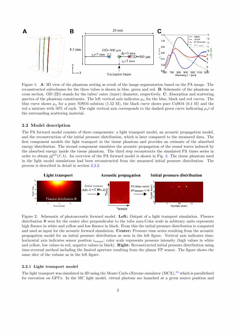
Figure 1: A: 3D view of the phantom setting as result of the image segmentation based on the PA image. Thereconstructed subvolumes for the three tubes is shown in blue, green and red. B: Schematic of the phantom ascross section. OD (ID) stands for the tubes’ outer (inner) diameter, respectively. C: Absorption and scatteringspectra of the phantom constituents. The left vertical axis indicates µa for the blue, black and red curves. Theblue curve shows µa for a pure NiSO4 solution (1.52 M), the black curve shows pure CuSO4 (0.4 M) and thered a mixture with 50% of each. The right vertical axis corresponds to the dashed green curve indicating µs′ ofthe surrounding scattering material.

2.2 Model description

The PA forward model consists of three components: a light transport model, an acoustic propagation model,and the reconstruction of the initial pressure distribution, which is later compared to the measured data. Thefirst component models the light transport in the tissue phantom and provides an estimate of the absorbedenergy distribution. The second component simulates the acoustic propagation of the sound waves induced bythe absorbed energy inside the tissue phantom. The third step reconstructs the simulated PA times series inorder to obtain psim0 (~r, λ). An overview of the PA forward model is shown in Fig. 2. The tissue phantom usedin the light model simulations had been reconstructed from the measured initial pressure distribution. Theprocess is described in detail in section 2.2.2.

Figure 2: Schematic of photoacoustic forward model. Left: Output of a light transport simulation. Fluencedistribution Φ seen for the center slice perpendicular to the tube axes.Color scale in arbitrary units representshigh fluence in white and yellow and low fluence in black. From this the initial pressure distribution is computedand used as input for the acoustic forward simulation. Center: Pressure time series resulting from the acousticpropagation model for an initial pressure distribution as seen in the left figure. Vertical axis indicates time;horizontal axis indicates sensor position rsensor; color scale represents pressure intensity (high values in whiteand yellow, low values in red, negative values in black). Right: Reconstructed initial pressure distribution usingtime-reversal method including the limited aperture resulting from the planar FP sensor. The figure shows thesame slice of the volume as in the left figure.

2.2.1 Light transport model

The light transport was simulated in 3D using the Monte Carlo eXtreme simulator (MCX),12 which is parallelizedfor execution on GPUs. In the MC light model, virtual photons are launched at a given source position and

3

propagated as packets of energy through a volume defined by a regular grid of isotropic voxels. In this model,photons are launched according to a beam profile, which is of similar shape as a 2-dimensional Gaussian curve.Photons are scattered according to the scattering coefficient µs and the anisotropy parameter g of the currentvoxel (defined by its material type). Photons deposit energy in a voxel when leaving that voxel, therebydecreasing the weight of that photon packet according to the absorption coefficient of that voxel. The packetweight deposited in the current voxel is added to its probability distribution, from which the absorbed energydistribution H and fluence Φ is calculated according to:

H(~r, λ) = µa(~r, λ)Φ(~r, λ).

The input to an MCX simulation was a volume file containing 400 × 400 × 130 voxels identifying onematerial type for each voxel. For each material type, the absorption coefficient µa, the scattering coefficient µs,the anisotropy parameter g, and the refractive index n are given as input parameters. Each voxel has a size of703 µm3, hence the total simulated volume is 28× 28× 9 mm3. In order to avoid limited volume effects on theresulting fluence (due to photons interacting with the volume boundaries), the light transport was simulatedusing a larger volume than the measured PA image, as studied in section 2.4. Four types of media were usedin the simulations presented here, one homogeneous background (diluted milk), for which we assume that theabsorption coefficient equals µa(λ) of water. The scattering coefficient of the background is represented bythe green curve in Fig. 1 C. The remaining three material types correspond to the three tubes, for which awavelength independent scattering coefficient of µs = 0.01 mm−1 and wavelength dependent µa(λ) as in Fig. 1C has been assumed.

For the comparison between measured and modeled data described in section 3.1, the values for µa(λ)were computed according to the known ratio of NiSO4 and CuSO4 solutions in the tubes. Pure solutions hadconcentrations of cmax

NiSO4 = 1.52 mol/liter and cmaxCuSO4 = 0.4 mol/liter, respectively. Hence, µa(λ) was computed

for tube k using the known absorption spectra αNiSO4(λ), αCuSO4(λ), respectively, and the known mixtureparameter Rk. Furthermore, we assumed that both substances contribute linearly to the total absorptioncoefficient:

µa,k(λ,Rk) = Rk · cmaxNiSO4αNiSO4(λ) + (1−Rk) · cmax

CuSO4αCuSO4(λ), (1)

where R1 = 0.75 for tube 1, R2 = 0.5 for tube 2 and R3 = 0.25.

For the parameter estimation procedure described in section 3.2, Rk and (thereby also µa) is consideredunknown and varied during the parameter search. An overview of the optical parameters used for the differentstudies is given in Table 1.

Table 1: List of optical parameters

material µa [mm−1] µs [mm−1] n g Type of study

background (1) µH20a (λ) µs(λ) see Fig. 1 C 1.33 0.9

Comparison measuredvs modeled data

tubes (2) µa(λ) see Fig. 1 C 0.1 1.33 0.9Comparison measured

vs modeled databackground (1) 2e− 2 10 1 0.9 Boundary conditionstubes (2) 5 10 1 0.9 Boundary conditions

For each MC light simulation we used 5 ·107 photons, which took approximately 1–2 minutes per simulationon a desktop GPU.19 As µa(λ) and µs(λ) are wavelength dependent, each measured wavelength requires acorresponding simulation of the light model for that particular parameter set. For the parameter search describedin section 3.2 the number of photons was reduced to 5 · 106 to speed up the parameter estimation procedure.

The output of the light transport model is the absorbed energy distribution H(~r, λ), from which the initialpressure distribution is computed using the Gruneisen parameter Γ:

4

p0(~r, λ) = ΓH(~r, λ).

For simplicity we assumed a Gruneisen coefficient of 1 for all materials. The initial pressure distributionp0(~r, λ) gained from the result of a MC simulation serves as input to the acoustic propagation model, whichwill be described in section 2.2.3.

2.2.2 Image segmentation

The goal of the image segmentation is to reconstruct the geometry of the tubes from the measured pressuredata. This way, the number of unknowns in the inversion scheme is reduced. That is, we do not seek thechromophore concentration at every voxel independently, but only for a small number of material types, whosecontinuous location were obtained through image segmentation. The optical parameters within one materialtype are assumed homogeneous.

The image segmentation applied here is not a framework that is generally applicable, e.g. to vessel networks.but rather represents a simple method using prior knowledge in order to proof the applicability of our model-based inversion approach. The input to the image segmentation is the initial pressure distribution pexp0 (~r)reconstructed from the measured pressure time-series for one excitation wavelength.

The image segmentation is based on the idea to search for local maxima in slices of pexp0 perpendicular to thetube axes and to draw filled circles around the local maxima representing the tube centers. For this purpose,we make use of prior knowledge regarding the number, the shape, and the geometry of the tube absorbers.

First, a gaussian blur filter with σ = 2 voxels is applied to the raw data pexp0 (~r) in order to reduce the impactof noise on the location of the local maxima. Then, the locations of three local maxima are extracted for eachslice of pexp0 perpendicular to the tube axes. The location of the maxima within one slice are assumed to representthe centers of the tubes. Around each local maximum, a filled circle with a radius of three voxels is drawnmarking the voxels belonging to that tube. The reconstructed tubes resulting from our image segmentationapproach are shown in Fig. 1 A with the original pressure data in gray. The result of the image segmentationis a volume identifying four different media types, which serves as input to the MC light transport simulations.

2.2.3 Acoustic propagation model

The input to the acoustic propagation model is the absorbed energy distribution pMCX0 (~r) obtained from

the results of the MC light transport simulations. The acoustic propagation model is simulated using the k-Wave toolbox16 for Matlab. Its purpose is to account for the limited aperture inherent to the planar detectorgeometry14,15 and its influence on the PA images. Homogeneous acoustic properties are assumed with a speedof sound of 1500 m/s and a density of 1000 kg/m

3. The computational grid used by k-Wave was initialized

with a spatial resolution of 70 µm and the standard temporal resolution defined by the sound speed. The initialpressure distribution psim0 (~r, λ) is obtained using k-Wave’s time-reversal method kspaceFirstOrder3DG and isaccelerated by execution on a GPU. The result of the time-reversal based reconstruction psim0 (~r, λ) is used forcomparison with the measured pressure distribution pexp0 (~r) shown in section 3.1.

2.3 Parameter estimation

The parameter estimation framework aims to determine the relative concentrations of NiSO4 and CuSO4solutions in the tube phantom, represented by the parameters Rk, k = 1, 2, 3 in Eq. 1. Our approach is basedon the comparison of PA spectra from measured and modeled data and the iterative update of the relativeconcentration in the model, depending on the residual difference between the PA spectra and the previouslytested parameters. An overview of the approach is shown in Fig. 3. As the MC light model does not provideany analytical form for the fluence (and hence the pressure distribution), the possibility to compute gradientsanalytically is not given. Hence, we use an iterative, non-gradient optimization for the parameter estimation,which is described in the following. First, PA spectra are obtained from multi-wavelength simulations using theMC light model. Obtaining the PA spectra from the acoustic propagation model was omitted for the sake ofexecution speed, but yielded equal final concentrations (not shown).

5

Figure 3: This schematic gives an overview of the workflow to obtain the relative concentration ratios in thethree phantom tubes. One instance of the PA forward model includes simulations of the light transport model,acoustic propagation and reconstruction for all Nλ wavelengths. For each tube k, the measured spectrum isfitted to the simulated spectrum using a linear scaling parameter βk. The sum of differences between the spectra∆Fitk is used to guide the parameter search (see Eq. 2 and 3). If the minimum sum of differences has beenfound, the concentration ratios in the tubes R∗ is estimated from the optical parameters {µa,1, . . . , µa,k } usedto obtain the minimal sum of differences. If the minimum is not yet found, the concentrations are updatedaccording to the coordinate search algorithm.

The PA spectra are computed by averaging the reconstructed pressure distribution psim0 (~r, λ) over all voxelsbelonging to a tube.This provides a mean PA signal psim0 (k, λ, µa,k) for tube k using a relative concentrationof absorbers Rk, which yields µa,k according to Eq. 1. The experimental PA signal pexp0 (k, λ) is averaged usingthe same voxels as to obtain psim0 . In order to compare the modeled and measured spectra, the measured PAspectrum is fitted to the simulated one through least squares minimization using a scalar scaling (or calibration)factor βk and the following error functional is used:

∆Fitk(Rk) =

Nλ∑

i=1

(βk · pexp0 (k, λi)− psim0 (k, λi, Rk))2. (2)

In order to find the optimal parameters for all tubes, we use a coordinate descent algorithm,20 where therelative concentration Rk in one tube represents one dimension. During the coordinate descent, the geometricparameters of the tubes and the optical properties of the background remain fixed. The only parameters that arebeing varied are the concentration parameters Rk for the three tubes, that determine the absorption coefficientµa,k (see Eq. 1).

The error landscape during the parameter search is determined by the sum of residuals (sum over all tubes):

E(R) =

Nk=3∑

k=1

∆Fitk(Rk), R = (R1, R2, R3) (3)

During the parameter search, the concentration parameters Rk are updated for each tube iteratively andindependently. In brief, the search is initialized using any (random) values for R. Furthermore, a directionvk for each dimension k and a global step size h are initialized. As long as the error (Eq. 3) decreased, Rk is

6

updated accordingly Rk = Rk + vk · h. The direction of the search is changed when the overall error E hasincreased. If the direction along the current dimension Rk has already been changed, the optimum along thenext dimension is sought. If the minimum along all three dimensions has been found with the current step sizeh, h is decreased (e.g. by a factor 2) and the search continues with the first tube, thereby trying to find the Rkthat minimizes the difference between PA spectra for the first tube (Eq. 2). As stop criterion we used the totalnumber of steps and whether a minimum step size has been reached. The values of R during the search areused to avoid multiple visits of the same location in the parameter space. If a location has been visited, anotherlocation in the same direction is sampled, while staying within the boundaries of Rk = (0, 1) . The progressduring and the results of the parameter search is shown in section 2.3 and Fig. 8.

2.4 Evaluation of Monte-Carlo light model

An important prerequisite in qPAT is the validation of methods underlying the quantification of chromophoreconcentrations. In a model-based approach, this involves answering the question which model parametersinfluence the solution that is being compared to measured data. When using MC simulations, naturally only alimited volume can be simulated in order to gain the solution within the region of interest (ROI). However, thischoice regarding the position of the boundaries, i.e. how large the simulated volume is or how far the boundariesare situated from the ROI, can affect the solution within the ROI.

Here, in preparation for the quantitative estimation of concentration ratios, we address two important issuesconcerning the setup of the MC light model simulations: First, we study the question as to how large thesimulated volume needs to be in order to exclude boundary effects on the fluence distribution inside the ROI,representing the size of measured PA images. Second, the effect of absorbers in the background (outside theROI) on the solution within the ROI is investigated.

The first question is addressed by simulating a phantom model using varying volume sizes while keeping thephantom model (i.e. the ROI) in the center of the simulated volume. The phantom consists of multiple tubesarranged in a grid of four layers with optical parameters very similar to the one used for the comparison ofexperimental data and the parameter estimation (see Table 1). A schematic of the setting is shown in Fig. 4 A,B, C.

The region of interest was defined as a cube with an edge length of 20 mm corresponding to the imagedvolume size in the PA measurements. The simulated volume was increased in several steps to a maximum sizeof 503 mm3, and the fluence distribution inside the tubes (averaged over the tube’s cross section) was used asa measure to test convergence (see Fig. 4 D). We observed that the influence of the boundary condition on thefluence distribution inside the tubes is stronger with increasing depth. This is due to the fact that the fluenceat greater depths is strongly determined by scattered light and photons that have interacted with the volumeboundary if the boundary is close to the ROI. Hence, the fluence distribution inside a tube in the deepest layerwas used as measure to test convergence (indicated by the yellow cross in Fig. 4 B). We found that convergencewithin the region of interest (ROI) was achieved by adding a boundary region that approximately doubled thetotal volume of the model (see Fig. 4, D). Consequently, the MC model in the inversion (section 3) included anadditional boundary region in order to exclude these boundary effects due to limited volume size. The boundaryregion had identical optical parameters as the background inside the ROI.

The second question, the effect of background absorbers on the fluence distribution within the ROI, wasaddressed by comparing two settings, shown in Fig. 5 A. In one setting, the grid of absorbing tubes extendedinto the additional boundary region, in the other setting the tubes were truncated and remained inside the ROI.Again, we compared the fluence distribution in a tube at a depth of 7 mm averaged over the tube’s cross sectionto study the influence of the background. The result is shown in Fig. 5 B. In the case with truncated tubes,the fluence shows a strong increase near the ROI boundaries which extends even into the ROI, compared to thesetting with continuous tubes. This effect is due to the light scattered in the additional boundary region, whichacts as a light source leading to an increased absorption at the endings of the truncated tubes. In contrast, inthe setting with continuous tubes, there is no sharp transition between strongly absorbing and weakly absorbingmaterials. In this setting, photons are absorbed by the continuous tubes when leaving the ROI. This leads toa difference in the fluence distribution between the two settings and shows that absorbers outside the ROI doaffect the solution within the ROI.

7

Figure 4: MC light model validation. A: Front view of the experimental setting used for the MC light modelevaluation. The profile of the excitation beam is shown in yellow and red (yellow representing high intensity).The parts of the tubes lying within the ROI are colored in blue. Tube parts extending outside the ROI areshown in green. The maximum dimensions of the simulated volume is 500 × 500 × 500 voxel, or 503mm3 B:Phantom setting viewed from above. The dimensions of the ROI is 200×200×200 voxel, or 203mm3. The yellowcross indicates the tube whose fluence distribution is shown in D. C: Distinction between ROI and backgroundvolume for the same perspective as in B. D: Effect of boundary conditions on fluence within one tube at a depthof 7 mm indicated by the yellow cross in B. The fluence is shown along the tube axis averaged over the tubecross section of one central tube. The ROI is depicted in gray. The differently colored curves represent resultsusing different surrounding volumes, where Nx = 200 means that no additional surrounding volume has beenused.

3. RESULTS

3.1 Comparison of experimental data with model

For a qualitative validation of the PA forward model, the measured and modeled reconstructed initial pressuredistributions pexp0 (~r, λ) and psim0 (~r, λ) are compared. For this purpose, we used the known optical properties for

8

Figure 5: Effect of background absorbers. A: Truncated (top) and continuous tubes (bottom) B: Fluencewithin a tube averaged over cross section for the two settings shown in A.

the tubes and for the scattering background material (see Table 1) in the two-stage PA model. A comparisonof the measured data, the MC light model output, and the modeled PA image is shown in Fig. 6. A slice inthe center of the volume orthogonal to the tube axes shows that the PA image reproduces the limited apertureartifacts (see Fig. 6 A, C). This also becomes visible in horizontal profiles seen in Fig. 6 D, showing data along aline of voxels in the center of the volume, orthogonal to the tube axes and the excitation beam direction (indicatedby the horizontal line in Fig. 6 A-C). It can be seen that the PA image does not capture all artifacts (negativep0 values) that are visible in the measured data pexp0 . The reason for the missing artifacts are likely acousticinhomogeneities21 or the interaction between pressure waves and the FPI detector, which are not modeled bythe acoustic propagation model. Still, the artifacts visible along the excitation beam direction (z-axis) shownin Fig. 6 E are well reproduced in the PA image. The curves shown in Fig. 6 D-F have been normalized totheir respective maximum. Thus, the two-stage PA forward model shows good qualitative agreement with themeasured data.

In order to compare the PA forward model to measured data in a quantitative way, we compare the PAspectra obtained through averaging the pexp0 (~r, λ) and psim0 (~r, λ) over all voxel belonging to the tubes. The PAspectra pexp0 and psim0 were measured and simulated using seven wavelengths between 614 nm and 930 nm. Asthe FPI detects pressure signals using voltage signals from a photodiode, a quantitative comparison requiresa calibration or scaling factor between modeled and measured pressure values. This calibration factor wasobtained by fitting the measured PA spectra to the modeled spectra using the least squared method with ascalar factor, see Eq. 2. A comparison of the measured and predicted PA spectra for all three tubes is shown inFig. 7.

3.2 Parameter estimation

The aim of the parameter estimation is to determine the concentration parameterRk for all three tubes k = 1, 2, 3(see Eq. 1) representing the relative concentration of NiSO4 and determining the optical properties of the tubes.For this purpose, the PA spectra from simulations and measurements were compared using a least squares fitbetween the two as described in section 2.3. The objective function E as given by Eq. 3 is sampled iteratively bysimulating one PA spectrum (comprising seven wavelengths) at a time using the MC light model. The value ofR (and thereby the µa,k) are updated after each iteration depending on the previous search and how the value

9

Figure 6: Measured and modeled PA images and intensity profiles: A: Measured cross sectional PA imageof the phantom, B: Initial pressure distribution obtained using the MC model, C: Cross sectional PA imagepredicted using the forward model, D: Image intensity profiles corresponding to the dashed horizontal lines inA)-C), E: Image intensity profiles corresponding to dash-dot lines in A)-C), F: Image intensity profile of alonga tube in x-direction averaged over the tube cross section.

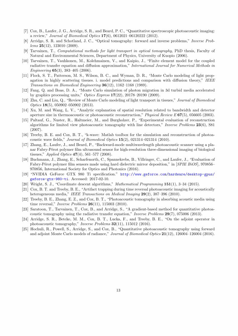
of E has changed. The objective function E is a three dimensional function where each dimension representsthe concentration parameter Rk for one tube. A one- and two-dimensional representation of E is shown inFig. 8 A and B, respectively. The two-dimensional error landscape in Fig. 8 B has been interpolated usingcubic interpolation based on 11 × 11 evenly spaced samples for the two parameter R1 and R3. The progressof the coordinate descent is shown in Fig. 8 B and C. In Fig. 8 B, the parameter search is initialized withR = 0, which is indicated by the black cross at R1,2 = (0, 0). There, sampled values of the parameter space areindicated by crosses with the gray value representing the progress, where black represents the beginning, grayindicate intermediate samples and white represents the final convergence of the search. The real concentrationis indicated by the yellow diamond at (0.766, 0.273), and the final values are represented by the white cross inFig. 8 B. In the course of the parameter search, the error measure E (evaluated with the currently best valuesof R) is decreasing monotonously, as shown in Fig. 8 C.

A comparison of the values obtained by the coordinate descent parameter search and the real values is givenin Table 2.

Table 2: Estimated relative concentrations. Results have been obtained running a coordinate search where therelative NiSO4 concentration in one tube represents one dimension.

Relative NiSO4 concentrationTube 1 Tube 2 Tube 3

Estimated concentration R∗ 79.7 % 56.2 % 29.0 %Known concentration 76.6 % 51.7 % 27.3 %

10

Figure 7: Measured and predicted PA spectra: PA image intensity was averaged over the respective tubevolumes. The spectra were fitted using least-squares with a linear scaling factor. Dashed lines indicate themeasured spectra, solid lines indicate simulated spectra. The blue curves correspond to tube 1, which contains76.6 % NiSO4; the red curves correspond to tube 2 with 51.7 % NiSO4; the black curves correspond to tube 3with 27.3 % NiSO4.

4. DISCUSSION

In this study, we presented a model-based inversion scheme for the estimation of absorber concentration ratios.The model comprises a two stage approach with a MC light transport model and acoustic propagation model.TheMC light model has been evaluated with respect to boundary conditions and background absorbers. It has beenfound that background absorbers influence the solution of the fluence inside the region of interest. The parameterestimation was based on the comparison between measured and modeled PA spectra and a coordinate descentparameter search with decreasing step size. The parameter search yielded an agreement between estimatedand known concentration values within 5%. The remaining difference arises from the minor mismatch in thePA spectra, which is likely due to an incomplete representation of the experimental setting in the PA model.Inaddition, effects of different Gruneisen parameters for different tubes could have contributed to the mismatch.Furthermore, in the PA model presented here, acoustic absorption22 and attenuation were not considered. Thesefactors, as well as acoustic heterogeneities,21 which were not included in the model, could explain the remainingmismatch between measured and modeled data and the incomplete representation of artifacts that has beenobserved.

Despite the promising results obtained with the parameter estimation framework presented here, furtherwork is required to retrieve the absolute concentration of absorbers, which is an important issue for futureresearch. A limitation of the presented approach is based on the image segmentation employed here, whichrequires prior knowledge regarding absorber geometries, which is not known for more complex settings includingdata obtained from tissue. Nevertheless, our aim was not to provide a general solution for image segmentationproblems occurring in PAT, but rather to present an initial proof-of-concept that reducing the number ofunknowns using image segmentation and thereby allowing the use of a gradient-free parameter search.

The parameter estimation approach presented here is based on the fact that the MC light model does not

11

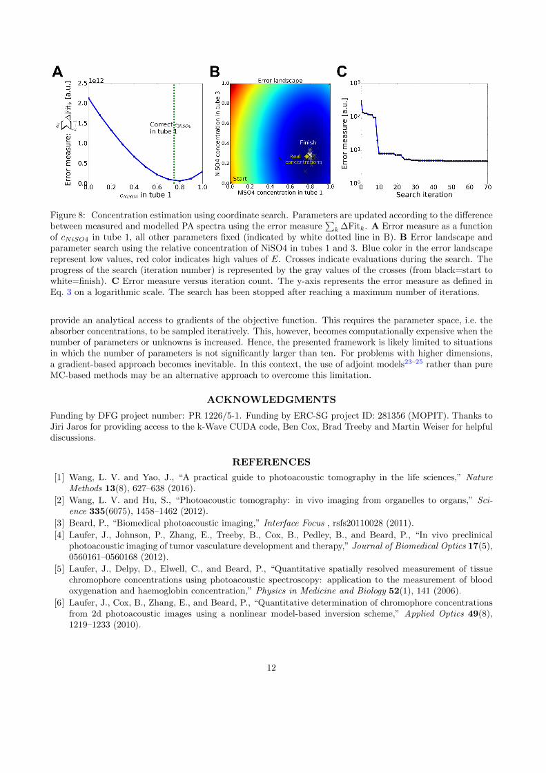
Figure 8: Concentration estimation using coordinate search. Parameters are updated according to the differencebetween measured and modelled PA spectra using the error measure

∑k ∆Fitk. A Error measure as a function

of cNiSO4 in tube 1, all other parameters fixed (indicated by white dotted line in B). B Error landscape andparameter search using the relative concentration of NiSO4 in tubes 1 and 3. Blue color in the error landscaperepresent low values, red color indicates high values of E. Crosses indicate evaluations during the search. Theprogress of the search (iteration number) is represented by the gray values of the crosses (from black=start towhite=finish). C Error measure versus iteration count. The y-axis represents the error measure as defined inEq. 3 on a logarithmic scale. The search has been stopped after reaching a maximum number of iterations.

provide an analytical access to gradients of the objective function. This requires the parameter space, i.e. theabsorber concentrations, to be sampled iteratively. This, however, becomes computationally expensive when thenumber of parameters or unknowns is increased. Hence, the presented framework is likely limited to situationsin which the number of parameters is not significantly larger than ten. For problems with higher dimensions,a gradient-based approach becomes inevitable. In this context, the use of adjoint models23–25 rather than pureMC-based methods may be an alternative approach to overcome this limitation.

ACKNOWLEDGMENTS

Funding by DFG project number: PR 1226/5-1. Funding by ERC-SG project ID: 281356 (MOPIT). Thanks toJiri Jaros for providing access to the k-Wave CUDA code, Ben Cox, Brad Treeby and Martin Weiser for helpfuldiscussions.

REFERENCES

[1] Wang, L. V. and Yao, J., “A practical guide to photoacoustic tomography in the life sciences,” NatureMethods 13(8), 627–638 (2016).

[2] Wang, L. V. and Hu, S., “Photoacoustic tomography: in vivo imaging from organelles to organs,” Sci-ence 335(6075), 1458–1462 (2012).

[3] Beard, P., “Biomedical photoacoustic imaging,” Interface Focus , rsfs20110028 (2011).

[4] Laufer, J., Johnson, P., Zhang, E., Treeby, B., Cox, B., Pedley, B., and Beard, P., “In vivo preclinicalphotoacoustic imaging of tumor vasculature development and therapy,” Journal of Biomedical Optics 17(5),0560161–0560168 (2012).

[5] Laufer, J., Delpy, D., Elwell, C., and Beard, P., “Quantitative spatially resolved measurement of tissuechromophore concentrations using photoacoustic spectroscopy: application to the measurement of bloodoxygenation and haemoglobin concentration,” Physics in Medicine and Biology 52(1), 141 (2006).

[6] Laufer, J., Cox, B., Zhang, E., and Beard, P., “Quantitative determination of chromophore concentrationsfrom 2d photoacoustic images using a nonlinear model-based inversion scheme,” Applied Optics 49(8),1219–1233 (2010).

12

[7] Cox, B., Laufer, J. G., Arridge, S. R., and Beard, P. C., “Quantitative spectroscopic photoacoustic imaging:a review,” Journal of Biomedical Optics 17(6), 0612021–06120222 (2012).

[8] Arridge, S. R. and Schotland, J. C., “Optical tomography: forward and inverse problems,” Inverse Prob-lems 25(12), 123010 (2009).

[9] Tarvainen, T., Computational methods for light transport in optical tomography, PhD thesis, Faculty ofNatural and Environmental Sciences, Department of Physics, University of Kuopio (2006).

[10] Tarvainen, T., Vauhkonen, M., Kolehmainen, V., and Kaipio, J., “Finite element model for the coupledradiative transfer equation and diffusion approximation,” International Journal for Numerical Methods inEngineering 65(3), 383–405 (2006).

[11] Flock, S. T., Patterson, M. S., Wilson, B. C., and Wyman, D. R., “Monte Carlo modeling of light prop-agation in highly scattering tissues. i. model predictions and comparison with diffusion theory,” IEEETransactions on Biomedical Engineering 36(12), 1162–1168 (1989).

[12] Fang, Q. and Boas, D. A., “Monte Carlo simulation of photon migration in 3d turbid media acceleratedby graphics processing units,” Optics Express 17(22), 20178–20190 (2009).

[13] Zhu, C. and Liu, Q., “Review of Monte Carlo modeling of light transport in tissues,” Journal of BiomedicalOptics 18(5), 050902–050902 (2013).

[14] Xu, M. and Wang, L. V., “Analytic explanation of spatial resolution related to bandwidth and detectoraperture size in thermoacoustic or photoacoustic reconstruction,” Physical Review E 67(5), 056605 (2003).

[15] Paltauf, G., Nuster, R., Haltmeier, M., and Burgholzer, P., “Experimental evaluation of reconstructionalgorithms for limited view photoacoustic tomography with line detectors,” Inverse Problems 23(6), S81(2007).

[16] Treeby, B. E. and Cox, B. T., “k-wave: Matlab toolbox for the simulation and reconstruction of photoa-coustic wave fields,” Journal of Biomedical Optics 15(2), 021314–021314 (2010).

[17] Zhang, E., Laufer, J., and Beard, P., “Backward-mode multiwavelength photoacoustic scanner using a pla-nar Fabry-Perot polymer film ultrasound sensor for high-resolution three-dimensional imaging of biologicaltissues,” Applied Optics 47(4), 561–577 (2008).

[18] Buchmann, J., Zhang, E., Scharfenorth, C., Spannekrebs, B., Villringer, C., and Laufer, J., “Evaluation ofFabry-Perot polymer film sensors made using hard dielectric mirror deposition,” in [SPIE BiOS ], 970856–970856, International Society for Optics and Photonics (2016).

[19] “NVIDIA GeForce GTX 980 Ti specification.” http://www.geforce.com/hardware/desktop-gpus/

geforce-gtx-980-ti. Accessed: 2017-02-10.

[20] Wright, S. J., “Coordinate descent algorithms,” Mathematical Programming 151(1), 3–34 (2015).

[21] Cox, B. T. and Treeby, B. E., “Artifact trapping during time reversal photoacoustic imaging for acousticallyheterogeneous media,” IEEE Transactions on Medical Imaging 29(2), 387–396 (2010).

[22] Treeby, B. E., Zhang, E. Z., and Cox, B. T., “Photoacoustic tomography in absorbing acoustic media usingtime reversal,” Inverse Problems 26(11), 115003 (2010).

[23] Saratoon, T., Tarvainen, T., Cox, B., and Arridge, S., “A gradient-based method for quantitative photoa-coustic tomography using the radiative transfer equation,” Inverse Problems 29(7), 075006 (2013).

[24] Arridge, S. R., Betcke, M. M., Cox, B. T., Lucka, F., and Treeby, B. E., “On the adjoint operator inphotoacoustic tomography,” Inverse Problems 32(11), 115012 (2016).

[25] Hochuli, R., Powell, S., Arridge, S., and Cox, B., “Quantitative photoacoustic tomography using forwardand adjoint Monte Carlo models of radiance,” Journal of Biomedical Optics 21(12), 126004–126004 (2016).

13