537KB - Computer Science and Mathematics Division - Oak

ORNL/TM-13338

Computer Science and Mathematics Division

Mathematical Sciences Section

RESULTS OF THE ANALYSIS OFTHE BLOOD LYMPHOCYTE PROLIFERATION TEST DATA

FROM THE NATIONAL JEWISH CENTER

E. L. Frome�

L.S. Newman†

M. M. Mroz †

� Mathematical Sciences SectionOak Ridge National LaboratoryOak Ridge, Tennessee 37831-0117

† National Jewish Center For Immunology andRespiratory MedicineDenver, Colorado

Date Published: March 1997

Research was supported by the Offices of Occupational Medicine, Envi-ronment, Safety and Health, U. S. Department of Energy

Prepared by theOak Ridge National LaboratoryOak Ridge, Tennessee 37831

managed byLockheed Martin Energy Research Corp.

for theU.S. DEPARTMENT OF ENERGY

under Contract No. DE-AC05-96OR22464

Contents

1 Introduction . . . . . . . . . . . . . . . . . . . . . . . . . . . . . . . . . . . . . . . 11.1 Description of Data From National Jewish Center . . . . . . . . . . . . . . . . 2

2 Estimation of SIs Using Least Absolute Values Method . . . . . . . . . . . . . . . . 32.1 Regression Model for the LPT Data . . . . . . . . . . . . . . . . . . . . . . . 32.2 Least Absolute Value Regression on Log(y) . . . . . . . . . . . . . . . . . . . 3

3 Identification of LPTs With Large SIs . . . . . . . . . . . . . . . . . . . . . . . . . 53.1 Method 1- Using Distribution of Maximum SI From Nonexposed Controls

and/or Historical Population of Beryllium Exposed Workers . . . . . . . . . . 53.2 Method 1A- Using Distribution of Second Largest SI From Nonexposed Con-

trols and/or Historical Population of Beryllium Exposed Workers . . . . . . . . 63.3 Method 2- Using The Empirical Distribution of log(SI)s For Each Day and

Each Beryllium Concentration . . . . . . . . . . . . . . . . . . . . . . . . . . 64 Results . . . . . . . . . . . . . . . . . . . . . . . . . . . . . . . . . . . . . . . . . . 7

4.1 Descriptive Statistics for Control Wells . . . . . . . . . . . . . . . . . . . . . . 74.2 Graphical Summaries for SIs For Beryllium Exposed Workers and Nonexposed

People . . . . . . . . . . . . . . . . . . . . . . . . . . . . . . . . . . . . . . . 114.3 Resistant Estimates of the Coefficient of Variation (φ) . . . . . . . . . . . . . 134.4 Identification Of LPTs With Large SIs . . . . . . . . . . . . . . . . . . . . . . 13

5 Comparison of The Three Methods . . . . . . . . . . . . . . . . . . . . . . . . . . . 245.1 Classification of Unacceptable LPTs . . . . . . . . . . . . . . . . . . . . . . . 25

5.1.1 Method 1 Results Based On Maximum SI . . . . . . . . . . . . . . . . 265.1.2 Method 1A Results Based On Second Largest SI . . . . . . . . . . . . 265.1.3 Method 2 Results Based On Each Day/Concentration . . . . . . . . . . 26

6 Criteria For Unacceptable LPTs . . . . . . . . . . . . . . . . . . . . . . . . . . . . 286.1 Criteria To Determine If Internal Variability Is Too High . . . . . . . . . . . . 28

6.1.1 Empirical Approach . . . . . . . . . . . . . . . . . . . . . . . . . . . 296.1.2 Theoretical Approach . . . . . . . . . . . . . . . . . . . . . . . . . . 296.1.3 Mathematical Analysis . . . . . . . . . . . . . . . . . . . . . . . . . . 296.1.4 Simulation Based Approach . . . . . . . . . . . . . . . . . . . . . . 30

7 Conclusions . . . . . . . . . . . . . . . . . . . . . . . . . . . . . . . . . . . . . . . 308 Acknowledgments . . . . . . . . . . . . . . . . . . . . . . . . . . . . . . . . . . . . 319 References . . . . . . . . . . . . . . . . . . . . . . . . . . . . . . . . . . . . . . . . 31A Detailed Report For LPT Data . . . . . . . . . . . . . . . . . . . . . . . . . . . . . 33

- iii -

List of Tables

1 Abnormal LPTs Using Method 1 For Sample of Beryllium Exposed Workers . 212 Abnormal LPTs Using Method 1A For Sample of Beryllium Exposed Workers 223 Abnormal LPTs Using Method 2 For Sample of Beryllium Exposed Workers . 234 Beryllium Exposed Workers Classified as Abnormal by at Least One Methoda . 245 Summary For NJC Unacceptable LPTs . . . . . . . . . . . . . . . . . . . . . . 256 Retest Summary Results For Method 1 . . . . . . . . . . . . . . . . . . . . . . 277 Summary RETEST Results For Method 1A . . . . . . . . . . . . . . . . . . . 278 Retest Summary Results For Method 2 . . . . . . . . . . . . . . . . . . . . . . 27

- v -

List of Figures

1 Day 5 Control Wells: Moment and Resistant Estimates—Linear Scale. . . . . . 82 Nonexposed and Beryllium Exposed Workers-Sample. Log-Log Plots For Day

5 and Day 7 Control Wells. . . . . . . . . . . . . . . . . . . . . . . . . . . . . 93 All Data Day 5 and Day 7 Control Wells- Log-Log Plots . . . . . . . . . . . . 104 Boxplots of SIs for Sample of Beryllium Exposed Workers and Controls . . . . 125 Normal Probability Plots of LAV Log(SI)s . . . . . . . . . . . . . . . . . . . 146 Normal Probability Plots For Nonexposed . . . . . . . . . . . . . . . . . . . . 157 SIs For Nonexposed (Controls) and Beryllium Exposed Workers . . . . . . . . 168 Resistant Estimates ofφ (CV) . . . . . . . . . . . . . . . . . . . . . . . . . . 179 Normal Probability Plots For Log(φ) . . . . . . . . . . . . . . . . . . . . . . . 1810 Distributions of Maximum of Log(SI) For NJC Data Sets . . . . . . . . . . . . 19

- vii -

RESULTS OF THE ANALYSIS OFTHE BLOOD LYMPHOCYTE PROLIFERATION TEST DATA

FROM THE NATIONAL JEWISH CENTER

E. L. Frome

L.S. Newman

M. M. Mroz

Abstract

A new approach to the analysis of the blood beryllium lymphocyte proliferation test(LPT) was presented to the Committee to Accredit Beryllium Sensitization Testing-BerylliumIndustry Scientific Advisory Committee in April, 1994. Two new outlier resistant meth-ods were proposed for the analysis of the blood LPT and compared with the approachthen in use by most labs. The method based on a least absolute values (LAV) analysis ofthe log of the well counts was recommended for routine use. It was considered impor-tant to “field test” the method on a new data base from another laboratory, since resultswere obtained using data from a single laboratory—Oak Ridge Institute for Science andEducation (ORISE).

The National Jewish Center (NJC) agreed to provide data (similar to that from ORISEin ORNL-6818) from a study that was underway at that time. Three groups of LPT dataare considered; i) a sample of 168 beryllium exposed (BE) workers and 20 nonexposed(NE) persons; ii) 25 unacceptable LPTs, and iii) 32 abnormal LPTs for individuals knownto have chronic beryllium disease (CBD). The LAV method described in ORNL-6818 wasapplied to each LPT. Graphical and numerical summaries similar to those presented forthe ORISE data are given. Three methods were used to identify abnormal LPTs. All threemethods correctly identified the 32 known CBD cases as abnormal. Results of applyingthe three methods to the BE-sample and Unacceptable data sets are presented, and resultsfor each of the three methods for the 20 Unacceptable LPTs and retest results are given.

These results support the earlier recommendation that the LAV method is a simple andeffective method for routine analysis of the blood beryllium LPT that is not effected byoutliers.

- ix -

1. Introduction

On April 22, 1994 a new approach to the analysis of the blood beryllium lymphocyte pro-

liferation test (LPT)1 was presented at the Committee to Accredit Beryllium Sensitization

Testing-Beryllium Industry Scientific Advisory Committee meeting in Washington, D.C. The

details of the method are described2 by Fromeet al in a research report (ORNL-6818) [4] and

were presented on November 8, 1994 at theConference on Beryllium Related Diseases[5]. At

the meeting there was general satisfaction with the proposed methods, but it was considered

important to “field test” the method on a new data base from another laboratory—results in

ORNL-6818 were obtained using data from the Oak Ridge Institute for Science and Education

(ORISE) laboratory. The National Jewish Center (NJC) agreed to provide data similar to that

in ORNL-6818 from a study that was underway at that time.

In ORNL-6818 two outlier resistant methods were proposed for the estimation of the stim-

ulation index (SI), which is the ratio of the response of beryllium stimulated cells to control

cells. These outlier resistant methods were compared with the approach then in use by most

labs. The method based on a least absolute values (LAV) analysis (Section 2.2) of the log of the

well counts was recommended for routine use.In this report all of the results are based on

the LAV method. All LPTs showed an adequate response to concanavalin-A (ConA) and

phytohemagglutinin (PHA) and those with obvious “laboratory error” (i.e. many wells

with no response above background) have been eliminated.

1Abbreviations used: AB,abnormal; Be,beryllium; BE,beryllium exposed; CBD,chronic beryllium dis-ease; ConA,concanavalin-A; CV,coefficient of variation; df,degrees of freedom; LAV,least absolute values;LPT,lymphocyte proliferation test; NE,nonexposed; NJC,National Jewish Center; ORISE,Oak Ridge Institute forScience and Education; ORNL,Oak Ridge National Laboratory; PHA,phytohemagglutinin; SI,stimulation index;UN,unacceptable;

2On the Internet see URL: http://www.epm.ornl.gov/ frome/BeLPT/index.html

- 2 -

1.1. Description of Data From National Jewish Center

Three groups of LPT data are considered:

� LPTs for a sample of 168 beryllium exposed (BE) workers

and 20 nonexposed (NE) persons.

� 25 unacceptable (UN) LPTs, and

� 32 abnormal (AB) LPT data sets.

The sample data consists of the first 168 persons whose blood arrived at NJC for beryllium

testing as part of a recent study and are considered to be representative of the study cohort.

One LPT from the beryllium exposed workers was removed because of laboratory error (eight

of twelve control wells showed background counts). The nonexposed LPT data are from 20

people who have no known beryllium exposure or respiratory disorders. These 20 LPTs were

performed by a single NJC technician.

The unacceptable data are from 25 patients who have “high variability” in their beryllium

test results or control cells. Data are flagged as unacceptable for any of the following reasons:

� three or more of the six beryllium stimulated groups are excluded due to high variation

� more than five control well data values are excluded due to high variation,

� ConA and PHA SIs are low (indicating low cell viability), or

� cell control counts are judged to be too high or too low (indicating possible contamina-

tion, failure to pulse, or other laboratory error).

High variation is defined in several ways. For beryllium stimulated quadruplicates (groups

of four at a particular beryllium concentration), values are rank ordered and the coefficient of

variation (CV) is calculated. If the CV is greater than 30%, the value farthest from the mean

is dropped and the CV is recalculated. If the CV for the remaining three values is still above

30%, the group is excluded. Three or more excluded groups is considered high variation.

High variation for cell control groups is the same as for beryllium stimulated groups with one

exception. It is defined as more than five control well counts excluded from the group without

achieving an acceptable CV.

- 3 -

The abnormal data are from 32 patients who have clinically confirmed beryllium disease

or beryllium sensitivity. The data are considered abnormal if two or more SIs exceed the

technician’s cut-off value. The cut-off value is two standard deviations above the mean peak

SI for nonexposed people.

2. Estimation of SIs Using Least Absolute Values Method

Results in this report are based on the LAV method described in detail in ORNL-6818. The

main results are summarized here.

2.1. Regression Model for the LPT Data

Let yjk denote the well count for thekth replicate of thejth set of culture conditions. The

expected count in each well can be represented by a log-linear regression function:

E(yjk) = λ j = exp(Xjβ); (1)

where j = 1; : : : ;10 andk = 1; : : : ;12 for the controls andk = 1;2;3;4 for the beryllium stim-

ulated cells and the positive controls. In (1),Xj is a row vector of indicator variables andβ is

the vector of regression parameters (see below). It is further assumed that the variance of the

well counts is proportional to the square of the expected count:

Var(yjk) = (φλ j)2: (2)

Equations 1 and 2 together are referred to as a generalized linear model with constant coeffi-

cient of variationφ (see ORNL-6818 for more details)

2.2. Least Absolute Value Regression on Log(y)

The first step in this approach is to take the log of the counts since this is the variance-stabilizing

transformation and leads to a linear model in sayzjk = log(yjk), i.e.

E(zjk) = Xjβ�φ2=2 andVar(zjk)' φ2:

In this report all logs are natural (base e) logarithms.If outliers are not present, applying

ordinary least squares to the transformed data will yield consistent estimates for the log(SI)

parameters [7]. The effect of outliers is minimized by using least absolute values (or some

- 4 -

other robust method) on thezjk. Least absolute value regression—also known as L1 norm,

least absolute deviations and minimum sum of absolute errors—is well known to be resistant

to outliers and is an important particular case of a general class of robust methods known as

M-estimators [10, 9]. In general, LAV regression requires special computational resources to

calculate parameter estimates [1]. In this situation, however, it is only necessary to find the

median of the log of the well counts for each set of design conditions and then subtract the

control median for each harvest day from the beryllium stimulated medians (see Appendices

ORNL-6818). Let ˜zj denote the median for thejth beryllium concentration and ˜zo denote the

median of the log well counts for beryllium stimulated cells and the corresponding control

wells. The LAV estimate of thejth log(SI), β j , is

β j = zj � zo: (3)

A resistant estimate of the coefficient of variation (φ) can then be obtained as

φ =C�medianfjzjk � zj jg; (4)

whereC = 1:48�p

n=(n� p), n = number of wells, andp = the number of medians. On

the log scaleφ corresponds to the standard deviation of the log counts. For the overall pooled

estimaten = 48 andp = 8 in this report. The value ofC is chosen to make the estimate

consistent for the standard deviation for a Gaussian error model and for consistency with the

usual least squares results in which the estimated variance is multiplied by the correction factor

n=(n� p) – see [6] and S-PLUS functionmad in [12]. Alternative approaches to estimating

φ have been discussed in the context of LAV regression (see e.g., [11, 9]) and there is no

consensus as to the best approach. In addition to the fact that this parameter is of direct interest

in this situation, it is also needed to obtain an estimate of the parameter covariance matrix

w2(X0X)�1;

wherew2 = [2 f (0)]�2 is the asymptotic variance of the sample median [2]. Following the

approach of [8] we assume that the underlying error distribution is Gaussian in the center and

usew=p

π=2φL to obtain an estimate of the standard deviation of the log of the stimulation

indices. The appropriate diagonal term from(X0X)�1 is 4=12, and consequently the estimated

standard deviation of log(SI) is 1:25φL(0:58) = 0:72φL.

- 5 -

3. Identification of LPTs With Large SIs

This section describes three approaches to the the problem of identification of an “abnormal”

LPT. Each of these methods uses the LAV estimatesβ j , j= 1,...,6, of the log(SI)s and resistant

estimates ofφ. Note that β j is a statistical shorthand for the LAV estimate of thejth log(SI).

3.1. Method 1- Using Distribution of Maximum SI From Nonexposed Controls and/orHistorical Population of Beryllium Exposed Workers

This approach parallels that currently in use for identification of LPTs with large SIs. The

procedure is to use the distribution of the maximum log(SI) in areference data baseof LPT data

sets to determine a “cut point”. The reference data base could be composed of LPTs for a group

of nonexposed individuals, or nonexposed plus historical data from beryllium exposed workers

with no indication of beryllium sensitivity. In this report there are LPTs for 20 nonexposed

individuals, and these, alone or in combination with the sample of 167 beryllium exposed

workers, will serve as the reference data base. The individuals with abnormal LPTshave not

been removed. The methods we use are outlier resistant and should be effective as long as the

proportion of abnormal LPTs in the study population is not too large.3 An LPT is considered

abnormal ifat least two log(SI)s exceed this cut point. The steps for this procedure are as

follows:

1. Findβ�

i = max[βi j ; j = 1; : : : ;6] for i = 1; : : : ;N, whereN= number of LPTs inreferencedata base.

2. FindM = median[β�

i ; i = 1; : : : ;N] and S the median absolute deviation (MAD) estimateof the standard deviation of theβ�

i .

3. Then calculatecut = M + zpS, wherezp is thepth quantile of the standard normal distri-bution. If p= 0.975 thenzp � 2.

4. An LPT is defined to beabnormal if at least two log(SI)s exceed cut.

The probability of a statistical false positive for this procedure is less than 1-p.

3If the reference data base is restricted to NE individuals, then the moment estimates of location and scale couldbe used instead of the resistant estimates. This approach is based on the assumption that there are no berylliumsensitive individuals in the NE group.

- 6 -

3.2. Method 1A- Using Distribution of Second Largest SI From Nonexposed Controlsand/or Historical Population of Beryllium Exposed Workers

This approach is the same as Method 1 except the second largest log(SI) in areference data

baseof LPT data sets is used to determine the “cut point”. An LPT is considered abnormal if

the second largestlog(SI) exceeds this cut point. The steps for this procedure are as follows:

1. Findβ†i = secondlargest[βi j ; j = 1; : : : ;6] for i = 1; : : : ;N, whereN= number of LPTs in

reference data set.

2. FindM = median[β†i ; i = 1; : : : ;N] and S the median absolute deviation (MAD) estimate

of the standard deviation of theβ†i .

3. Then calculatecut = M + zpS, wherezp is thepth quantile of the standard normal distri-bution. If p= 0.975 thenzp = 1.96.

4. An LPT is defined to beabnormal if at least two log(SI)s exceed cut.

The probability of a false positive for this procedure should be about 1-p.

3.3. Method 2- Using The Empirical Distribution of log(SI)s For Each Day and EachBeryllium Concentration

The third approach is the one proposed in Section 3.6 of ORNL-6818. It is based on the

assumption that the log(SIs) are approximately normally distributed (see Figures 5 and 6).In

this report the reference data base consists of all available LPTs in the BE-sample data

set and the NE data set.In practice this data set would change during the course of a study

as new data becomes available.The first step is to convert each log(SI) into a standardized

deviate

ui j =βi j � µj

sj

using the values of ˜µj andsj given in Table 3. These standardized deviates can be compared

with the quantiles of the standard normal distribution, i.e. Pr[u< zp] = p. If we assume that the

log(SIs) are independent then the binomial distribution can be used to calculate an approximate

probability of at leastk out of six “large” SIs for a given value ofzp. The probability of at least

one large SI is 1� p6, and the probability of at least two is 1� [p6+6(1� p)p5].

In fact, the log(SIs) are positively correlated, so this probability should be a lower bound

on the chance of finding a false positive LPT.

- 7 -

4. Results

4.1. Descriptive Statistics for Control Wells

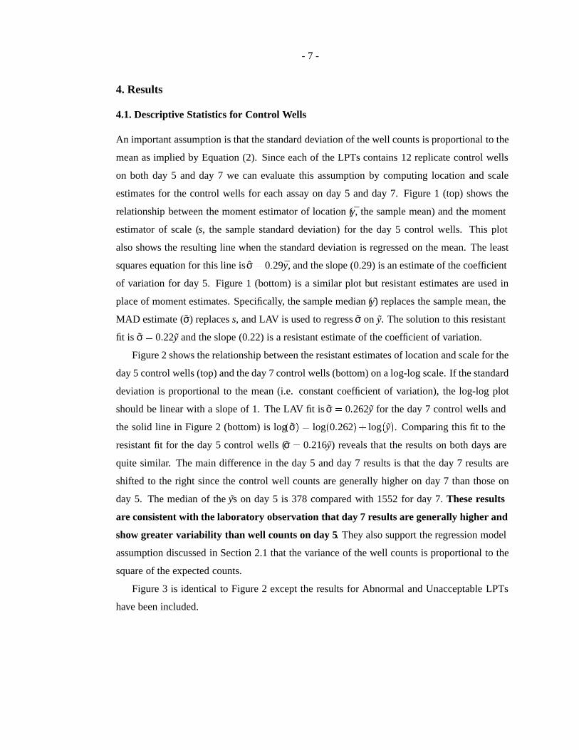
An important assumption is that the standard deviation of the well counts is proportional to the

mean as implied by Equation (2). Since each of the LPTs contains 12 replicate control wells

on both day 5 and day 7 we can evaluate this assumption by computing location and scale

estimates for the control wells for each assay on day 5 and day 7. Figure 1 (top) shows the

relationship between the moment estimator of location (¯y, the sample mean) and the moment

estimator of scale (s, the sample standard deviation) for the day 5 control wells. This plot

also shows the resulting line when the standard deviation is regressed on the mean. The least

squares equation for this line isσ = 0:29y, and the slope (0.29) is an estimate of the coefficient

of variation for day 5. Figure 1 (bottom) is a similar plot but resistant estimates are used in

place of moment estimates. Specifically, the sample median ( ˜y) replaces the sample mean, the

MAD estimate (σ) replacess, and LAV is used to regressσ on y. The solution to this resistant

fit is σ = 0:22y and the slope (0.22) is a resistant estimate of the coefficient of variation.

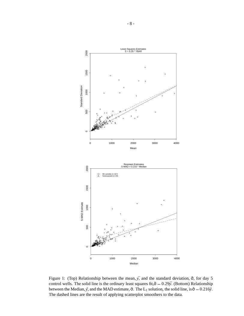
Figure 2 shows the relationship between the resistant estimates of location and scale for the

day 5 control wells (top) and the day 7 control wells (bottom) on a log-log scale. If the standard

deviation is proportional to the mean (i.e. constant coefficient of variation), the log-log plot

should be linear with a slope of 1. The LAV fit isσ = 0:262y for the day 7 control wells and

the solid line in Figure 2 (bottom) is log(σ) = log(0:262)+ log(y). Comparing this fit to the

resistant fit for the day 5 control wells (σ = 0:216y) reveals that the results on both days are

quite similar. The main difference in the day 5 and day 7 results is that the day 7 results are

shifted to the right since the control well counts are generally higher on day 7 than those on

day 5. The median of the ˜ys on day 5 is 378 compared with 1552 for day 7.These results

are consistent with the laboratory observation that day 7 results are generally higher and

show greater variability than well counts on day 5. They also support the regression model

assumption discussed in Section 2.1 that the variance of the well counts is proportional to the

square of the expected counts.

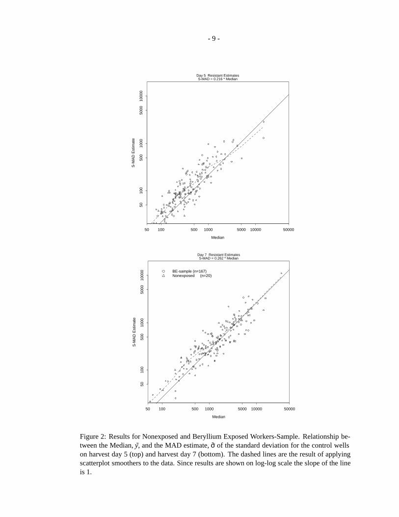
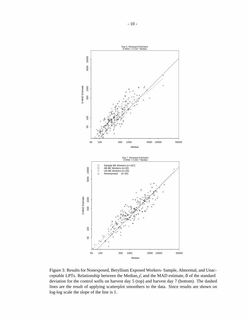
Figure 3 is identical to Figure 2 except the results for Abnormal and Unacceptable LPTs

have been included.

- 8 -

Mean

Sta

ndar

d D

evia

tion

0 1000 2000 3000 4000

050

010

0015

0020

00

Least Squares Estimates S = 0.29 * YBAR

Median

S-M

AD

Est

imat

e

0 1000 2000 3000 4000

050

010

0015

0020

00

BE-sample (n=167)Nonexposed (n=20)

Resistant Estimates S-MAD = 0.216 * Median

Figure 1: (Top) Relationship between the mean, ¯y, and the standard deviation,σ, for day 5control wells. The solid line is the ordinary least squares fit,σ = 0:29y. (Bottom) Relationshipbetween the Median, ˜y, and the MAD estimate,σ. The L1 solution, the solid line, isσ=0:216y.The dashed lines are the result of applying scatterplot smoothers to the data.

- 9 -

Median

S-M

AD

Est

imat

e

50 100 500 1000 5000 10000 50000

5010

050

010

0050

0010

000

Day 5 Resistant Estimates S-MAD = 0.216 * Median

Median

S-M

AD

Est

imat

e

50 100 500 1000 5000 10000 50000

5010

050

010

0050

0010

000


BE-sample (n=167)Nonexposed (n=20)

Figure 2: Results for Nonexposed and Beryllium Exposed Workers-Sample. Relationship be-tween the Median, ˜y, and the MAD estimate,σ of the standard deviation for the control wellson harvest day 5 (top) and harvest day 7 (bottom). The dashed lines are the result of applyingscatterplot smoothers to the data. Since results are shown on log-log scale the slope of the lineis 1.

- 10 -

Median

S-M

AD

Est

imat

e

50 100 500 1000 5000 10000 50000

5010

050

010

0050

0010

000


Median

S-M

AD

Est

imat

e

50 100 500 1000 5000 10000 50000

5010

050

010

0050

0010

000


Sample BE Workers (n=167)AB BE Workers (n=32)UN BE Workers (n=25)Nonexposed (n=20)

Figure 3: Results for Nonexposed, Beryllium Exposed Workers- Sample, Abnormal, and Unac-ceptable LPTs. Relationship between the Median, ˜y, and the MAD estimate,σ of the standarddeviation for the control wells on harvest day 5 (top) and harvest day 7 (bottom). The dashedlines are the result of applying scatterplot smoothers to the data. Since results are shown onlog-log scale the slope of the line is 1.

- 11 -

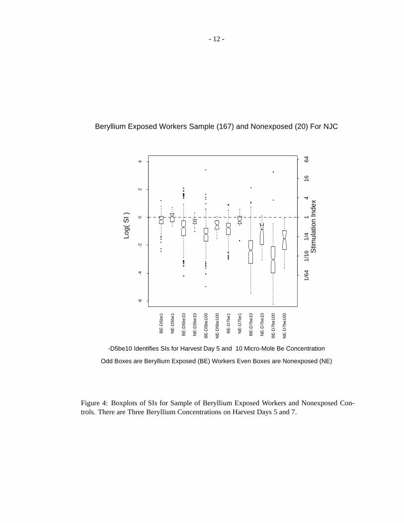
4.2. Graphical Summaries for SIs For Beryllium Exposed Workers and Nonexposed Peo-ple

Figure 4 shows the SIs for the sample of beryllium exposed (BE) workers and nonexposed

(NE) controls (compare with Fig. 4 for the ORISE-AC Data in Fromeet al. [5]). The vertical

scale on the right hand side of the plots is in SI units. The SIs for both the NE controls and the

beryllium exposed workers decrease as the beryllium concentration in the test wells increases.

This may be due to a toxic effect of high beryllium concentration that results in “cell killing”.

There is considerably more variability in the log(SI)s for the BE LPTs than for the NE LPTs at

each concentration on both day 5 and day 7.

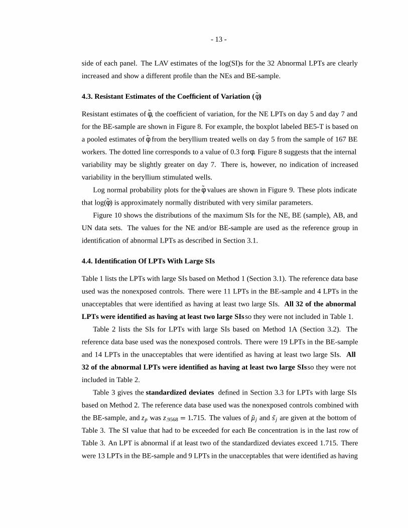
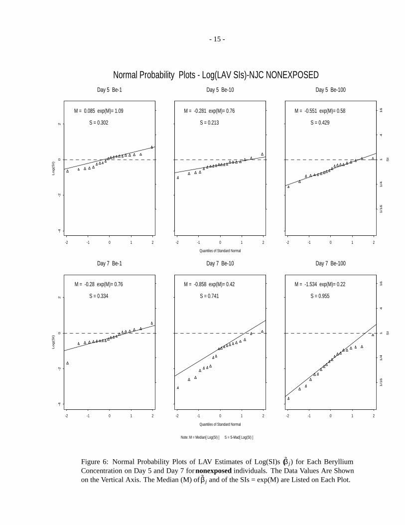
Figure 5 shows normal (Gaussian) probability plots for the combined BE and NE SIs for

each of the three beryllium concentrations on day 5 and day 7. In each of the six plots, the data

(ordered values of the log(SIs)) are shown on the vertical scale on the left, and the quantiles of

the standard normal distribution are shown on the horizontal scale. A detailed account of the

construction and interpretation of normal probability plots is provided by Chamberset .al [3].

In this situation statistical theory indicates that the log(SIs) should be approximately normally

distributed, and the large sample standard deviation should be about 0.28 if the coefficient

of variation is 0.4. If the relation between the empirical quantiles (on the vertical axis) and

theoretical quantiles (on the horizontal axis) is linear, this indicates that the distribution is

Gaussian. Each plot includes the median (labeled M) and a resistant estimate of the standard

deviation (labeled S) for the log SIs. The solid line in each plot shows the relation that is

expected if the log SI values are from a normal distribution with location parameter M (which

determines the intercept) and standard deviation S (which determines the slope). Resistant

methods were used to estimate the location and scale parameters for the combined data from

the BE and NE groups. This reflects the assumption that most of beryllium exposed workers

do not show an abnormal response, i.e. they look like the nonexposed group. For example,

consider the plot for day 5 Be-10 in Figure 5. The log(SIs) appear to be approximately normal

in the center, but there are several values that are larger than expected (these are the points

above the line). These “outliers” are SIs that indicate hypersensitivity to beryllium. Compare

these results to similar plots for the ORISE data—see [5] Fig. 5.

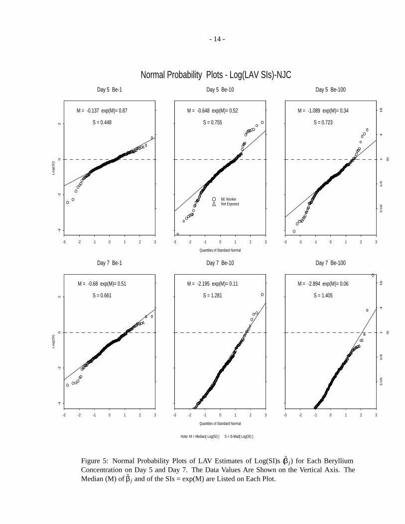
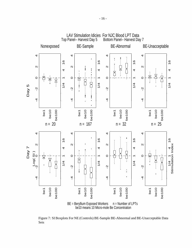
Normal probability plots for thenonexposedworkers alone are shown in Figure 6. Box-

plots for each of the data sets considered in this report are shown in Figure 7. The top panel

contains results for day 5 and the bottom panel for day 7. The NE controls are shown on the left

- 12 -

-6-4

-20

24

BE

-D5b

e1

NE

-D5b

e1

BE

-D5b

e10

NE

-D5b

e10

BE

-D5b

e100

NE

-D5b

e100

BE

-D7b

e1

NE

-D7b

e1

BE

-D7b

e10

NE

-D7b

e10

BE

-D7b

e100

NE

-D7b

e100

Beryllium Exposed Workers Sample (167) and Nonexposed (20) For NJC

-D5be10 Identifies SIs for Harvest Day 5 and 10 Micro-Mole Be Concentration

Odd Boxes are Beryllium Exposed (BE) Workers Even Boxes are Nonexposed (NE)

1/64

1/16

1/4

14

1664

S

timul

atio

n In

dex

Log(

SI )

Figure 4: Boxplots of SIs for Sample of Beryllium Exposed Workers and Nonexposed Con-trols. There are Three Beryllium Concentrations on Harvest Days 5 and 7.

- 13 -

side of each panel. The LAV estimates of the log(SI)s for the 32 Abnormal LPTs are clearly

increased and show a different profile than the NEs and BE-sample.

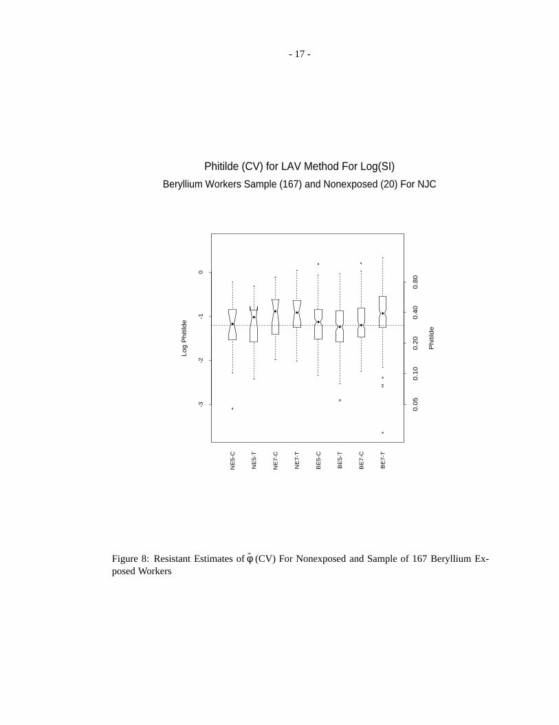
4.3. Resistant Estimates of the Coefficient of Variation (φ)

Resistant estimates ofφ, the coefficient of variation, for the NE LPTs on day 5 and day 7 and

for the BE-sample are shown in Figure 8. For example, the boxplot labeled BE5-T is based on

a pooled estimates ofφ from the beryllium treated wells on day 5 from the sample of 167 BE

workers. The dotted line corresponds to a value of 0.3 forφ. Figure 8 suggests that the internal

variability may be slightly greater on day 7. There is, however, no indication of increased

variability in the beryllium stimulated wells.

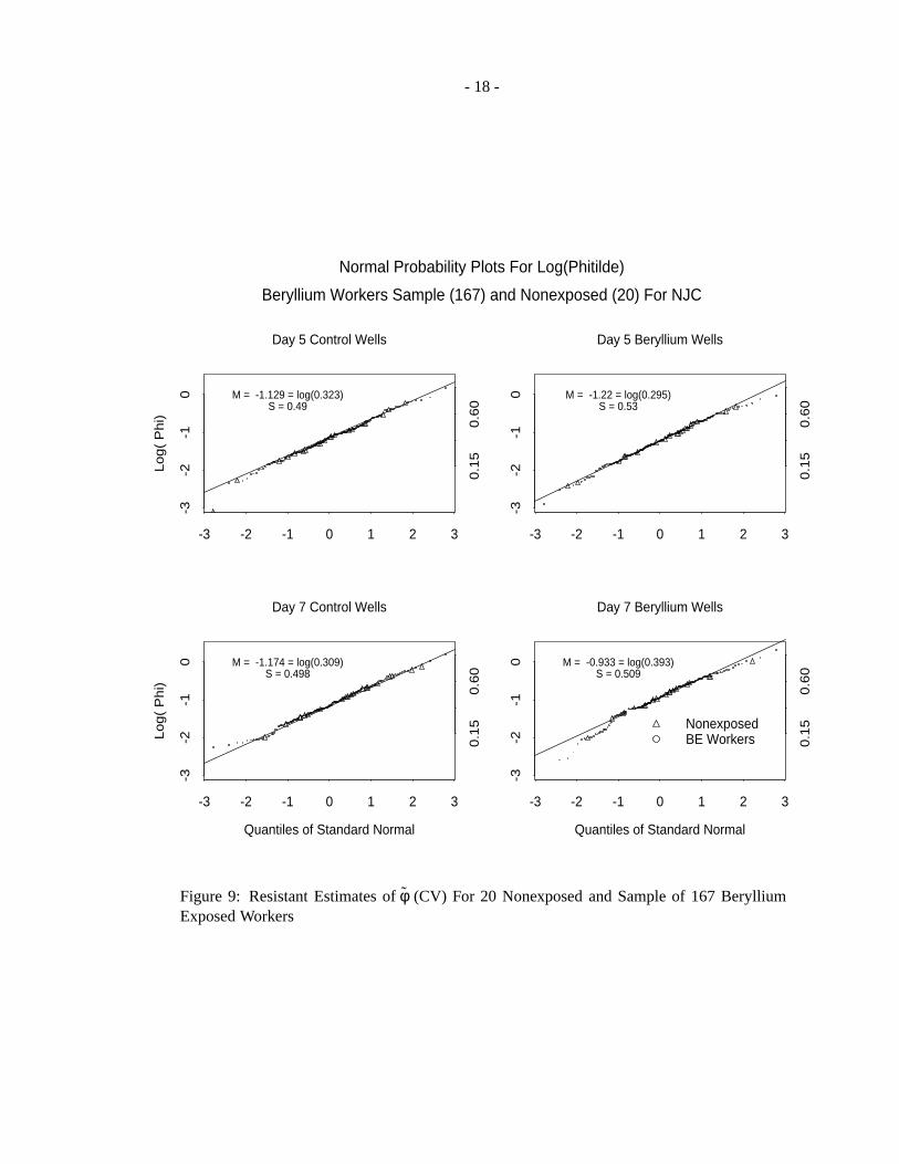
Log normal probability plots for theφ values are shown in Figure 9. These plots indicate

that log(φ) is approximately normally distributed with very similar parameters.

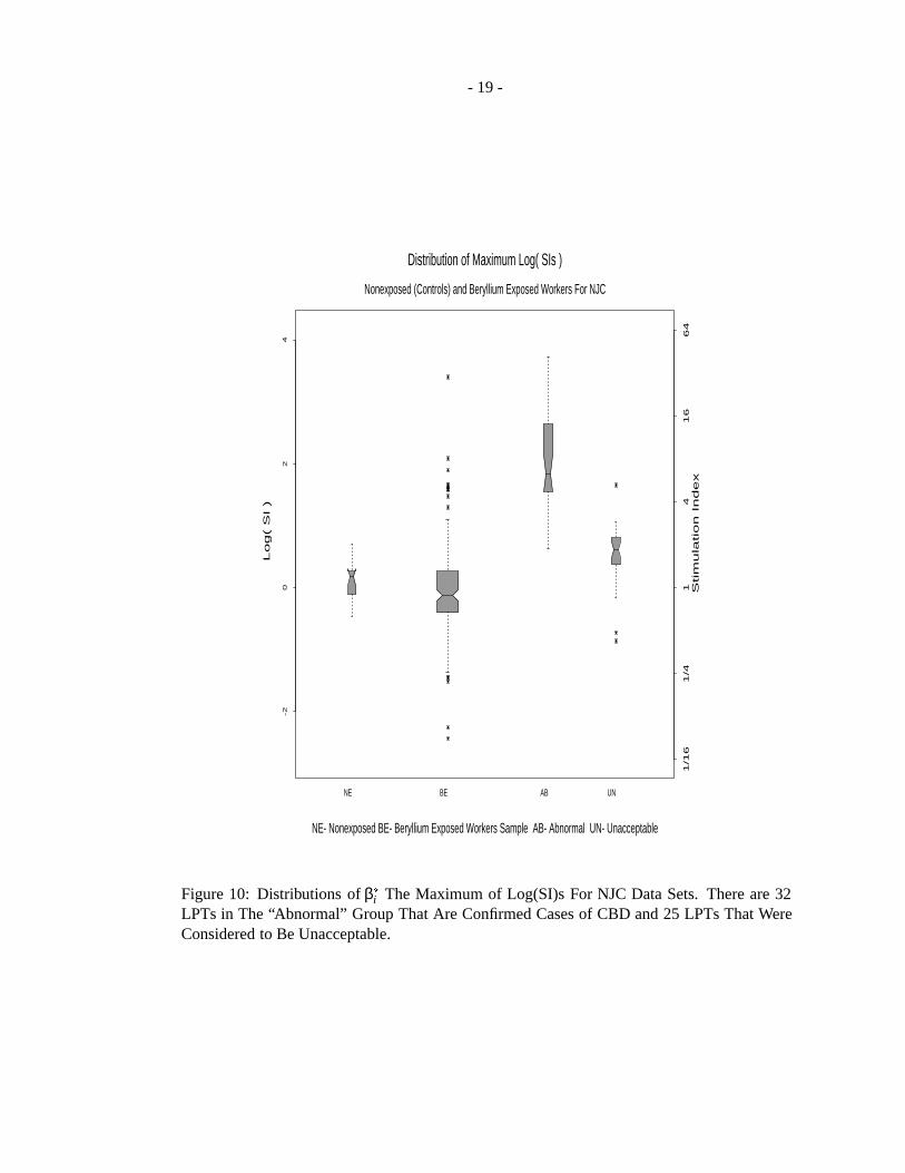
Figure 10 shows the distributions of the maximum SIs for the NE, BE (sample), AB, and

UN data sets. The values for the NE and/or BE-sample are used as the reference group in

identification of abnormal LPTs as described in Section 3.1.

4.4. Identification Of LPTs With Large SIs

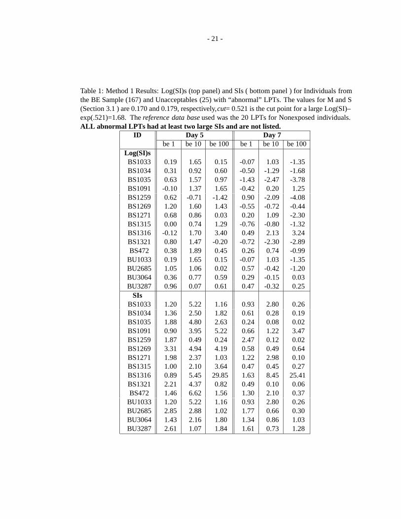
Table 1 lists the LPTs with large SIs based on Method 1 (Section 3.1). The reference data base

used was the nonexposed controls. There were 11 LPTs in the BE-sample and 4 LPTs in the

unacceptables that were identified as having at least two large SIs.All 32 of the abnormal

LPTs were identified as having at least two large SIsso they were not included in Table 1.

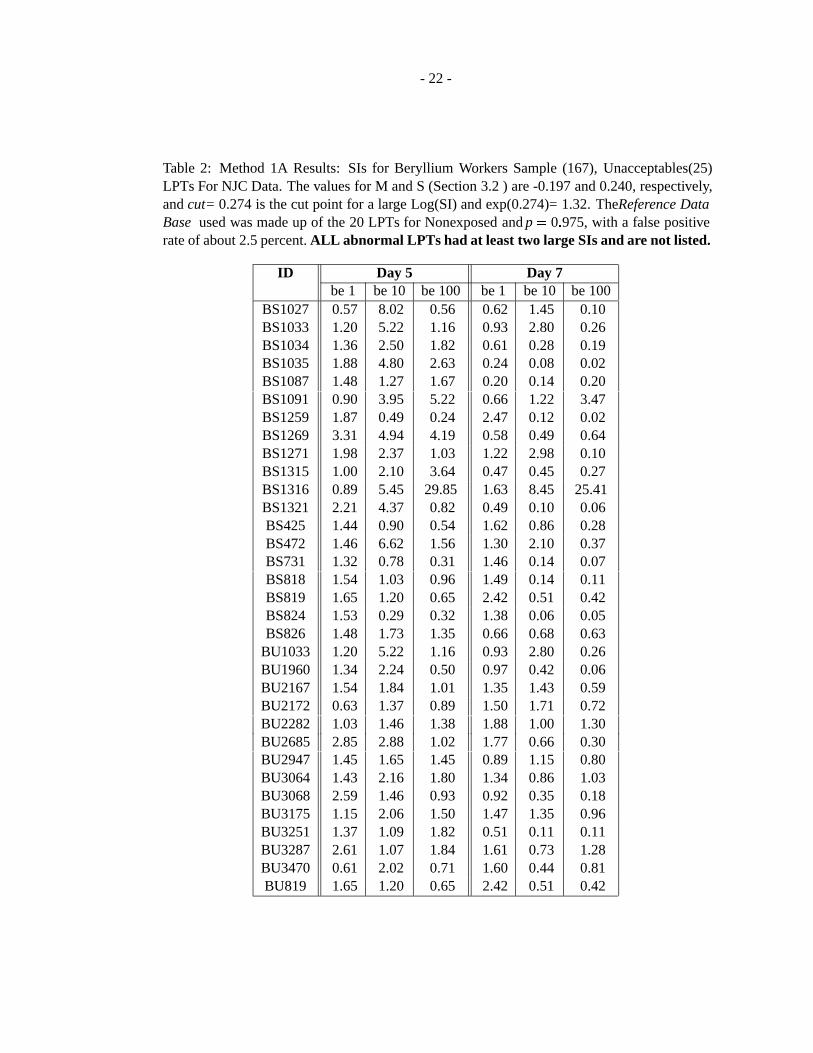
Table 2 lists the SIs for LPTs with large SIs based on Method 1A (Section 3.2). The

reference data base used was the nonexposed controls. There were 19 LPTs in the BE-sample

and 14 LPTs in the unacceptables that were identified as having at least two large SIs.All

32 of the abnormal LPTs were identified as having at least two large SIsso they were not

included in Table 2.

Table 3 gives thestandardized deviatesdefined in Section 3.3 for LPTs with large SIs

based on Method 2. The reference data base used was the nonexposed controls combined with

the BE-sample, andzp wasz:9568= 1:715. The values of ˜µj andsj are given at the bottom of

Table 3. The SI value that had to be exceeded for each Be concentration is in the last row of

Table 3. An LPT is abnormal if at least two of the standardized deviates exceed 1.715. There

were 13 LPTs in the BE-sample and 9 LPTs in the unacceptables that were identified as having

- 14 -

Log(S

I)

-3 -2 -1 0 1 2 3

-4-2

02

M = -0.137 exp(M)= 0.87

S = 0.448

Day 5 Be-1

Quantiles of Standard Normal

-3 -2 -1 0 1 2 3

Day 5 Be-10

M = -0.648 exp(M)= 0.52

S = 0.755

BE WorkerNot Exposed

-3 -2 -1 0 1 2 3

1/1

61/4

14

16

Day 5 Be-100

SI

M = -1.089 exp(M)= 0.34

S = 0.723

Log(S

I)

-3 -2 -1 0 1 2 3

-4-2

02

Day 7 Be-1

M = -0.68 exp(M)= 0.51

S = 0.661


-3 -2 -1 0 1 2 3

Day 7 Be-10

M = -2.195 exp(M)= 0.11

S = 1.281

-3 -2 -1 0 1 2 3

1/1

61/4

14

16

Day 7 Be-100

M = -2.894 exp(M)= 0.06

S = 1.405

Normal Probability Plots - Log(LAV SIs)-NJC

Note: M = Median[ Log(SI) ] S = S-Mad[ Log(SI) ]

SI

Figure 5: Normal Probability Plots of LAV Estimates of Log(SI)s (β j ) for Each BerylliumConcentration on Day 5 and Day 7. The Data Values Are Shown on the Vertical Axis. TheMedian (M) ofβ j and of the SIs = exp(M) are Listed on Each Plot.

- 15 -

Log(S

I)

-2 -1 0 1 2

-4-2

02

M = 0.085 exp(M)= 1.09

S = 0.302

Day 5 Be-1


-2 -1 0 1 2

Day 5 Be-10

M = -0.281 exp(M)= 0.76

S = 0.213

BE WorkerNonexposed

-2 -1 0 1 2

1/1

61/4

14

16

Day 5 Be-100

SI

M = -0.551 exp(M)= 0.58

S = 0.429

Log(S

I)

-2 -1 0 1 2

-4-2

02

Day 7 Be-1

M = -0.28 exp(M)= 0.76

S = 0.334


-2 -1 0 1 2

Day 7 Be-10

M = -0.858 exp(M)= 0.42

S = 0.741

-2 -1 0 1 2

1/1

61/4

14

16

Day 7 Be-100

M = -1.534 exp(M)= 0.22

S = 0.955

Normal Probability Plots - Log(LAV SIs)-NJC NONEXPOSED

Note: M = Median[ Log(SI) ] S = S-Mad[ Log(SI) ]

SI

Figure 6: Normal Probability Plots of LAV Estimates of Log(SI)s (β j ) for Each BerylliumConcentration on Day 5 and Day 7 fornonexposedindividuals. The Data Values Are Shownon the Vertical Axis. The Median (M) ofβ j and of the SIs = exp(M) are Listed on Each Plot.

- 16 -

-4-2

02

4

be

1

be

10

be

10

0

1/4

14

16

Nonexposed

-4-2

02

4

be

1

be

10

be

10

0

1/4

14

16

n = 20

Lo

g(

SI

)

-4-2

02

4

be

1

be

10

be

10

0

1/4

14

16

BE-Sample

-4-2

02

4

be

1

be

10

be

10

0

1/4

14

16

n = 167

-4-2

02

4

be

1

be

10

be

10

0

1/4

14

16

BE-Abnormal

-4-2

02

4

be

1

be

10

be

10

0

1/4

14

16

n = 32

-4-2

02

4

be

1

be

10

be

10

0

1/4

14

16

BE-Unacceptable

-4-2

02

4

be

1

be

10

be

10

0

1/4

14

16

n = 25

Stim

ula

tio

n I

nd

ex

LAV Stimulation Idicies For NJC Blood LPT DataTop Panel-- Harvest Day 5 Bottom Panel-- Harvest Day 7

BE = Beryllium Exposed Workers n = Number of LPTs be10 means 10 Micro-mole Be Concentration

Da

y 7

Da

y 5

Figure 7: SI Boxplots For NE (Controls) BE-Sample BE-Abnormal and BE-Unacceptable DataSets

- 17 -

-3-2

-10

NE

5-C

NE

5-T

NE

7-C

NE

7-T

BE

5-C

BE

5-T

BE

7-C

BE

7-T

Phitilde (CV) for LAV Method For Log(SI)

Beryllium Workers Sample (167) and Nonexposed (20) For NJC

0.0

50

.10

0.2

00

.40

0.8

0

Ph

itild

e

Lo

g P

hiti

lde

Figure 8: Resistant Estimates ofφ (CV) For Nonexposed and Sample of 167 Beryllium Ex-posed Workers

- 18 -

Log(

Phi)

-3 -2 -1 0 1 2 3

-3-2

-10

0.1

50.6

0

M = -1.129 = log(0.323)S = 0.49

Day 5 Control Wells

-3 -2 -1 0 1 2 3-3

-2-1

0

0.1

50.6

0

M = -1.22 = log(0.295)S = 0.53

Day 5 Beryllium Wells


Log(

Phi)

-3 -2 -1 0 1 2 3

-3-2

-10

0.1

50.6

0

M = -1.174 = log(0.309)S = 0.498

Day 7 Control Wells


-3 -2 -1 0 1 2 3

-3-2

-10

0.1

50.6

0

M = -0.933 = log(0.393)S = 0.509

Day 7 Beryllium Wells

Nonexposed BE Workers

Beryllium Workers Sample (167) and Nonexposed (20) For NJC

Normal Probability Plots For Log(Phitilde)

Figure 9: Resistant Estimates ofφ (CV) For 20 Nonexposed and Sample of 167 BerylliumExposed Workers

- 19 -

-20

24

NE BE AB UN

1/1

61/4

14

16

64

Stim

ula

tio

n I

nd

ex

L

og

( S

I )

Nonexposed (Controls) and Beryllium Exposed Workers For NJC

Distribution of Maximum Log( SIs )

NE- Nonexposed BE- Beryllium Exposed Workers Sample AB- Abnormal UN- Unacceptable

Figure 10: Distributions ofβ�

i The Maximum of Log(SI)s For NJC Data Sets. There are 32LPTs in The “Abnormal” Group That Are Confirmed Cases of CBD and 25 LPTs That WereConsidered to Be Unacceptable.

- 20 -

at least two large SIs.All 32 of the abnormal LPTs were identified as having at least two

large SIsso they were not included in Table 3. An approximate lower bound (see Section 3.3)

on the probability of a false positive is 1� [p6+6(1� p)p5] = :025.

- 21 -

Table 1: Method 1 Results: Log(SI)s (top panel) and SIs ( bottom panel ) for Individuals fromthe BE Sample (167) and Unacceptables (25) with “abnormal” LPTs. The values for M and S(Section 3.1 ) are 0.170 and 0.179, respectively,cut= 0.521 is the cut point for a large Log(SI)–exp(.521)=1.68. Thereference data baseused was the 20 LPTs for Nonexposed individuals.ALL abnormal LPTs had at least two large SIs and are not listed.

ID Day 5 Day 7be 1 be 10 be 100 be 1 be 10 be 100

Log(SI)sBS1033 0.19 1.65 0.15 -0.07 1.03 -1.35BS1034 0.31 0.92 0.60 -0.50 -1.29 -1.68BS1035 0.63 1.57 0.97 -1.43 -2.47 -3.78BS1091 -0.10 1.37 1.65 -0.42 0.20 1.25BS1259 0.62 -0.71 -1.42 0.90 -2.09 -4.08BS1269 1.20 1.60 1.43 -0.55 -0.72 -0.44BS1271 0.68 0.86 0.03 0.20 1.09 -2.30BS1315 0.00 0.74 1.29 -0.76 -0.80 -1.32BS1316 -0.12 1.70 3.40 0.49 2.13 3.24BS1321 0.80 1.47 -0.20 -0.72 -2.30 -2.89BS472 0.38 1.89 0.45 0.26 0.74 -0.99

BU1033 0.19 1.65 0.15 -0.07 1.03 -1.35BU2685 1.05 1.06 0.02 0.57 -0.42 -1.20BU3064 0.36 0.77 0.59 0.29 -0.15 0.03BU3287 0.96 0.07 0.61 0.47 -0.32 0.25

SIsBS1033 1.20 5.22 1.16 0.93 2.80 0.26BS1034 1.36 2.50 1.82 0.61 0.28 0.19BS1035 1.88 4.80 2.63 0.24 0.08 0.02BS1091 0.90 3.95 5.22 0.66 1.22 3.47BS1259 1.87 0.49 0.24 2.47 0.12 0.02BS1269 3.31 4.94 4.19 0.58 0.49 0.64BS1271 1.98 2.37 1.03 1.22 2.98 0.10BS1315 1.00 2.10 3.64 0.47 0.45 0.27BS1316 0.89 5.45 29.85 1.63 8.45 25.41BS1321 2.21 4.37 0.82 0.49 0.10 0.06BS472 1.46 6.62 1.56 1.30 2.10 0.37

BU1033 1.20 5.22 1.16 0.93 2.80 0.26BU2685 2.85 2.88 1.02 1.77 0.66 0.30BU3064 1.43 2.16 1.80 1.34 0.86 1.03BU3287 2.61 1.07 1.84 1.61 0.73 1.28

- 22 -

Table 2: Method 1A Results: SIs for Beryllium Workers Sample (167), Unacceptables(25)LPTs For NJC Data. The values for M and S (Section 3.2 ) are -0.197 and 0.240, respectively,andcut= 0.274 is the cut point for a large Log(SI) and exp(0.274)= 1.32. TheReference DataBase used was made up of the 20 LPTs for Nonexposed andp= 0:975, with a false positiverate of about 2.5 percent.ALL abnormal LPTs had at least two large SIs and are not listed.


BS1027 0.57 8.02 0.56 0.62 1.45 0.10BS1033 1.20 5.22 1.16 0.93 2.80 0.26BS1034 1.36 2.50 1.82 0.61 0.28 0.19BS1035 1.88 4.80 2.63 0.24 0.08 0.02BS1087 1.48 1.27 1.67 0.20 0.14 0.20BS1091 0.90 3.95 5.22 0.66 1.22 3.47BS1259 1.87 0.49 0.24 2.47 0.12 0.02BS1269 3.31 4.94 4.19 0.58 0.49 0.64BS1271 1.98 2.37 1.03 1.22 2.98 0.10BS1315 1.00 2.10 3.64 0.47 0.45 0.27BS1316 0.89 5.45 29.85 1.63 8.45 25.41BS1321 2.21 4.37 0.82 0.49 0.10 0.06BS425 1.44 0.90 0.54 1.62 0.86 0.28BS472 1.46 6.62 1.56 1.30 2.10 0.37BS731 1.32 0.78 0.31 1.46 0.14 0.07BS818 1.54 1.03 0.96 1.49 0.14 0.11BS819 1.65 1.20 0.65 2.42 0.51 0.42BS824 1.53 0.29 0.32 1.38 0.06 0.05BS826 1.48 1.73 1.35 0.66 0.68 0.63

BU1033 1.20 5.22 1.16 0.93 2.80 0.26BU1960 1.34 2.24 0.50 0.97 0.42 0.06BU2167 1.54 1.84 1.01 1.35 1.43 0.59BU2172 0.63 1.37 0.89 1.50 1.71 0.72BU2282 1.03 1.46 1.38 1.88 1.00 1.30BU2685 2.85 2.88 1.02 1.77 0.66 0.30BU2947 1.45 1.65 1.45 0.89 1.15 0.80BU3064 1.43 2.16 1.80 1.34 0.86 1.03BU3068 2.59 1.46 0.93 0.92 0.35 0.18BU3175 1.15 2.06 1.50 1.47 1.35 0.96BU3251 1.37 1.09 1.82 0.51 0.11 0.11BU3287 2.61 1.07 1.84 1.61 0.73 1.28BU3470 0.61 2.02 0.71 1.60 0.44 0.81BU819 1.65 1.20 0.65 2.42 0.51 0.42

- 23 -

Table 3: Method 2 Results: Standardized Deviates (see Section 3.3 ) For Beryllium ExposedWorkers and Unacceptable LPTs. The value ofp= 0:9568 so the false positive rate is about2.5 percent.ALL abnormal LPTs had at least two large SIs and are not listed.


BS1027 -0.94 3.62 0.70 0.31 2.00 0.41BS1033 0.72 3.05 1.71 0.92 2.52 1.10BS1034 0.99 2.07 2.33 0.28 0.71 0.86BS1035 1.72 2.94 2.85 -1.14 -0.22 -0.63BS1091 0.08 2.68 3.79 0.39 1.87 2.95BS1261 -0.20 2.97 0.75 0.21 1.75 0.57BS1269 2.98 2.97 3.49 0.20 1.15 1.74BS1271 1.83 2.00 1.54 1.33 2.57 0.42BS1315 0.31 1.84 3.29 -0.13 1.09 1.12BS1316 0.04 3.10 6.20 1.77 3.38 4.36BS1321 2.08 2.81 1.22 -0.06 -0.08 0.00BS472 1.15 3.36 2.12 1.43 2.29 1.35BS826 1.18 1.58 1.92 0.40 1.41 1.73

BU1033 0.72 3.05 1.71 0.92 2.52 1.10BU2172 -0.72 1.27 1.34 1.64 2.13 1.83BU2282 0.36 1.36 1.95 1.98 1.72 2.25BU2685 2.64 2.26 1.53 1.89 1.39 1.21BU2947 1.14 1.52 2.02 0.85 1.82 1.90BU3064 1.10 1.88 2.31 1.47 1.60 2.08BU3175 0.61 1.82 2.07 1.61 1.95 2.03BU3287 2.45 0.95 2.35 1.75 1.47 2.24BU3470 -0.79 1.79 1.03 1.74 1.07 1.91

Med -0.14 -0.65 -1.09 -0.68 -2.19 -2.89Smad 0.45 0.75 0.72 0.66 1.28 1.41Cut SI 1.88 1.91 1.16 1.57 1.00 0.62

- 24 -

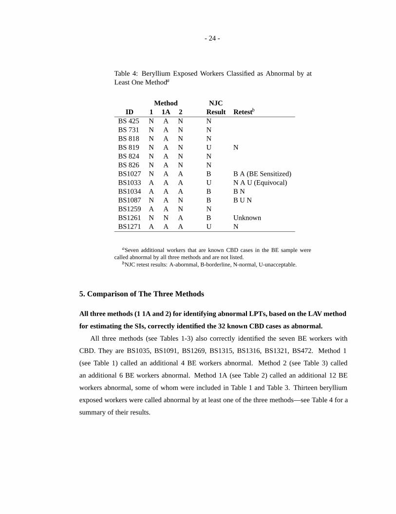
Table 4: Beryllium Exposed Workers Classified as Abnormal by atLeast One Methoda

Method NJCID 1 1A 2 Result Retestb

BS 425 N A N NBS 731 N A N NBS 818 N A N NBS 819 N A N U NBS 824 N A N NBS 826 N A N NBS1027 N A A B B A (BE Sensitized)BS1033 A A A U N A U (Equivocal)BS1034 A A A B B NBS1087 N A N B B U NBS1259 A A N NBS1261 N N A B UnknownBS1271 A A A U N

aSeven additional workers that are known CBD cases in the BE sample werecalled abnormal by all three methods and are not listed.

bNJC retest results: A-abornmal, B-borderline, N-normal, U-unacceptable.

5. Comparison of The Three Methods

All three methods (1 1A and 2) for identifying abnormal LPTs, based on the LAV method

for estimating the SIs, correctly identified the 32 known CBD cases as abnormal.

All three methods (see Tables 1-3) also correctly identified the seven BE workers with

CBD. They are BS1035, BS1091, BS1269, BS1315, BS1316, BS1321, BS472. Method 1

(see Table 1) called an additional 4 BE workers abnormal. Method 2 (see Table 3) called

an additional 6 BE workers abnormal. Method 1A (see Table 2) called an additional 12 BE

workers abnormal, some of whom were included in Table 1 and Table 3. Thirteen beryllium

exposed workers were called abnormal by at least one of the three methods—see Table 4 for a

summary of their results.

- 25 -

5.1. Classification of Unacceptable LPTs

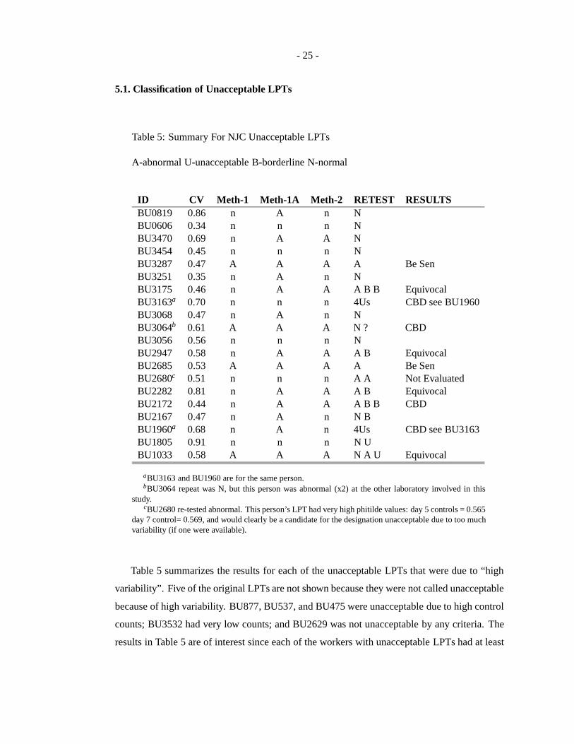
Table 5: Summary For NJC Unacceptable LPTs

A-abnormal U-unacceptable B-borderline N-normal

ID CV Meth-1 Meth-1A Meth-2 RETEST RESULTSBU0819 0.86 n A n NBU0606 0.34 n n n NBU3470 0.69 n A A NBU3454 0.45 n n n NBU3287 0.47 A A A A Be SenBU3251 0.35 n A n NBU3175 0.46 n A A A B B EquivocalBU3163a 0.70 n n n 4Us CBD see BU1960BU3068 0.47 n A n NBU3064b 0.61 A A A N ? CBDBU3056 0.56 n n n NBU2947 0.58 n A A A B EquivocalBU2685 0.53 A A A A Be SenBU2680c 0.51 n n n A A Not EvaluatedBU2282 0.81 n A A A B EquivocalBU2172 0.44 n A A A B B CBDBU2167 0.47 n A n N BBU1960a 0.68 n A n 4Us CBD see BU3163BU1805 0.91 n n n N UBU1033 0.58 A A A N A U Equivocal

aBU3163 and BU1960 are for the same person.bBU3064 repeat was N, but this person was abnormal (x2) at the other laboratory involved in this

study.cBU2680 re-tested abnormal. This person’s LPT had very high phitilde values: day 5 controls = 0.565

day 7 control= 0.569, and would clearly be a candidate for the designation unacceptable due to too muchvariability (if one were available).

Table 5 summarizes the results for each of the unacceptable LPTs that were due to “high

variability”. Five of the original LPTs are not shown because they were not called unacceptable

because of high variability. BU877, BU537, and BU475 were unacceptable due to high control

counts; BU3532 had very low counts; and BU2629 was not unacceptable by any criteria. The

results in Table 5 are of interest since each of the workers with unacceptable LPTs had at least

- 26 -

one additional LPT at NJC and the retest results are given in Table 5. Two of these (BU3163

and BU1960) are for the same person, a confirmed CBD case. Both of theφ values are very

high (0.70 and 0.68) and BU1960 was called abnormal by Method 1A.

One LPT that was called abnormal (BU3064) using LAV SIs by all three methods was

normal on retest by NJC, but was called abnormal twice at a second lab. BU2680 was called

normal using LAV estimates by all three methods, and was called abnormal in two retests at

NJC. The CBD status of this patient has not been evaluated.

5.1.1. Method 1 Results Based On Maximum SI

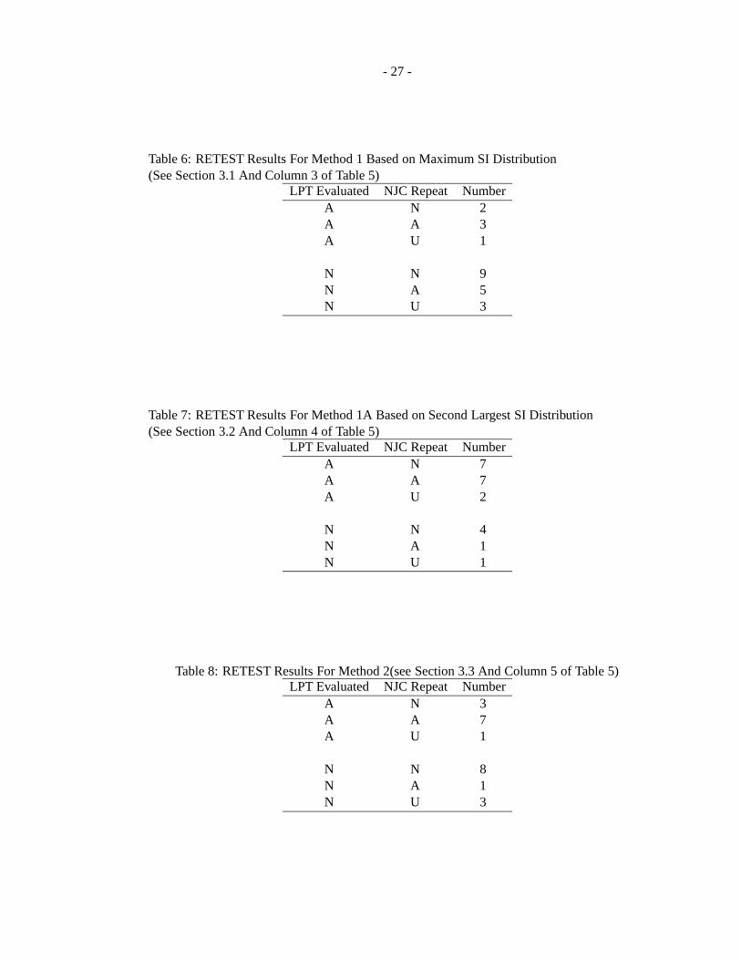
Table 6 summarizes the results of the retest LPTs that were done for each of the original

unacceptable LPTs using Method 1. For example, row two indicates that 3 of the Method

1 abnormal LPTs were abnormal on retest, and row five shows that 5 of the normal LPTs

were abnormal. This suggests that Method 1 may be missing some of the beryllium sensitized

individuals.

5.1.2. Method 1A Results Based On Second Largest SI


unacceptable LPTs using Method 1A. Row two indicates that seven of the Method 1A abnormal

LPTs were abnormal on retest, and only one of the normal LPTs was abnormal on retest (see

row 5). The first row of Table 7 shows that seven of the abnormals were normal on retest (based

on NJC method), suggesting that this method may have more false positive results.

5.1.3. Method 2 Results Based On Each Day/Concentration


unacceptable LPTs using Method 2. Seven of the eight abnormals were called abnormal on

retest, and only three of the abnormals were called normal.

Note that some NJC Unacceptables had more than one RETEST ( see Table 5) , and

all of the retest results were used to obtain Tables 6-8.

- 27 -

Table 6: RETEST Results For Method 1 Based on Maximum SI Distribution(See Section 3.1 And Column 3 of Table 5)

LPT Evaluated NJC Repeat NumberA N 2A A 3A U 1

N N 9N A 5N U 3

Table 7: RETEST Results For Method 1A Based on Second Largest SI Distribution(See Section 3.2 And Column 4 of Table 5)

LPT Evaluated NJC Repeat NumberA N 7A A 7A U 2

N N 4N A 1N U 1

Table 8: RETEST Results For Method 2(see Section 3.3 And Column 5 of Table 5)LPT Evaluated NJC Repeat Number

A N 3A A 7A U 1

N N 8N A 1N U 3

- 28 -

6. Criteria For Unacceptable LPTs

One feature of the LAV approach is that it is not necessary to declare LPTs as unacceptable

because of “high variability” in the well counts based on the CV. There are however situations

that may result in an unacceptable LPT. Data may be considered unacceptable if any of the

following situations occur:

1. Control well counts are too low or too high relative to plate background due to laboratoryerror. Sources of technical error might include mistakes in pipetting, such as failures toadd appropriate numbers of cells to individual wells, lack of addition or double additionof tritiated thymidine to specific wells, or improper washing of filters resulting in residualcounts of unincorporated thymidine, or smearing of radiolabel across the filter paper.

2. Positive control SIs for ConA or PHA SIs are low (indicating low cell viability).

3. The internal variability for a quadruplicate of Be stimulated cells is “too high” for at leasttwo Be concentrations, provided this is due to at least two counts that are “two low”, i.e.close to background for the plate indicating laboratory error— See Section 6.1.

4. The internal variability for the control wells is too high on day 5 or day 7. An approxi-mate critical value forφL can be obtained using an empirical or theoretical approach—see Section 6.1.

5. At least four SIs are “too low” indicating cell killing. An SI is too low if it is signifi-cantly below the null value of one (zero on the log scale). In Section 2.2 the theoreticalstandard deviation of log(SI) is 1:25φL(0:58) = 0:72φL. If φL = 0.30, then the standarddeviation of a log(SI) is 0.216. Since the Pr[log(SI) < 0:216zp] = p, then forp= 0.001,

Pr[log(SI) <�3:1�0:216] = Pr[log(SI) <�0:67] = 0:001,

i.e Pr[SI< 0:51] = 0.001.

The last item above may not be needed if it can be demonstrated that cell killing only

occurs among individuals who are not sensitized to beryllium.

6.1. Criteria To Determine If Internal Variability Is Too High

The resistant estimate of the CV (φL) is too high if it exceeds a critical value CV*. The value

of CV* can be obtained using an empirical or theoretical approach.

- 29 -

6.1.1. Empirical Approach

The empirical approach uses the distribution ofφL estimates available from previous data (see

e.g. Fromeet al.[4] page 13 and page 26). This method could be applied to the control well

counts on day 5 and day 7 (12 replicates per set). It could also be applied to the CV-mad

estimates obtained from the Be stimulated wells (4 replicates per set).

6.1.2. Theoretical Approach

Assume that the log (base e) counts follow the Gaussian distribution withknown φ. Then use

either mathematical analysis or simulation to determine a percentage point for the sampling

distribution ofφL. Recall thatφ is the standard deviation of the log of the counts, and cor-

responds to the CV on the original scale under the assumption that the standard deviation is

proportional to the mean on the original scale (see ORNL-6818 Section 2.1).

6.1.3. Mathematical Analysis

This approach can be applied to the usual moment estimate of the standard of the log counts,

i.e., NOT to the MAD estimate,φL. If SD is the moment estimate of the standard deviation for

a sample of size n of z(i)’s that are normally distributed withknown variance (i.e. φ2), then

the chi-square distribution can be used to determine a critical value of the moment estimate of

the standard deviation.

This should be a lower bound for the distribution of the resistant estimateφL. For example,

if φ =0.3, then for control wells (df= 11),

pr[ SD> 0.401 ] is about 0.05,

pr[ SD> 0.450 ] is about 0.01,

and, pr[ SD> 0.506 ] is about 0.001.

For the Be stimulated wells (df= 3), and

and pr[ SD> 0.48] is about 0.05,

and pr[ SD> 0.70 ] is about 0.001

The problem with this approach is that the distribution ofφL will be more spread out than

the distribution of the moment estimate of the standard deviation when the log counts follow

the Gaussian distribution.

- 30 -

6.1.4. Simulation Based Approach

An alternative is to use simulation to generate the sampling distribution of SD andφL. For a

given value ofφ generate say 10,000 samples of sizen (n= 4, 8, or 12). Calculate the value

of SD andφL for each sample and calculate the desired quantiles of the sampling distribution.

In the absence of outliers this should match the results based on the chi-square distribution for

SD, but the null distribution ofφL will be more spread out.

This same procedure can then be repeatedwith outliers being added, say ten percent of

the time, to each of the samples of sizen. This leads to a specified critical value forφL that will

depend on the value ofφ that is used, and on the proportion of outliers that is assumed.

7. Conclusions

Three methods were described for identification of an abnormal blood LPT using LAV esti-

mates of the SIs. These methods were applied to the BE-sample, Unacceptable, and Abnormal

data sets. All three methods correctly identified the 32 known CBD cases as abnormal, and

identified the seven known CBD cases in the BE-sample.

Results of applying the three methods to the BE-sample and Unacceptable data sets were

presented. Table 5 summarizes the results for each method for the 20 NJC Unacceptable LPTs,

gives the retest results and the evaluation of the patients’ CBD status. Both Method 2 and

Method 1A were effective at classifying beryllium sensitized individuals. Method 1A had

more results that were normal on retest by NJC using their usual criteria, i.e. the retest results

were not based on Method 1A using LAV approach. Method 2 used the combined data from

the NE (control) group and the BE worker group. Consequently, we cannot determine how

this method would have classified the unacceptable LPTs in a “real time” situation, since the

reference data basechanges as new data becomes available.

Figure 4 suggests that there was “cell killing” present at the two highest Be concentrations

on Day 5 and 7. Figure 5 and Figure 6 support the assumption that the log(SI)s are Gaussian

in the center.

Distributions of resistant estimates (φ) of the CV were presented—Figure 8. These results

show that the internal variability is similar for the BE-sample and NE-sample for control wells

and treated wells on days 5 and 7. These distributions are similar to those seen at ORISE and

are centered at aboutφ =0.30.

- 31 -

8. Acknowledgments

This research was supported by the Offices of Occupational Medicine, Environment, Safety

and Health, U. S. Department of Energy under contract DE-AC05-96OR22464 with Lockheed

Martin Energy Research Corp. The authors thank R. L Schmoyer, L. G. Littlefield, and S. P.

Colyer for reviewing this report, and R. L. Neubert for technical assistance with data prepara-

tion.

The work has been authored by a contractor of the U.S. Government. Accordingly, the U.S.

Government retains a nonexclusive, royalty-free license to publish or reproduce the published

form of this work, or to allow others to do so for U. S. Government purposes.

9. References

[1] R.A. Armstrong, E.L. Frome, and D.S. Kung. A revised simplex algorithm for the abso-lute deviation curve fitting problem.Commun. Statist., B8:175–190, 1979.

[2] G. Basset, Jr. and R. Koenker. Asymptotic theory of least absolute error regression.Journal of the American Statistical Association, 73:618–622, 1978.

[3] J.M. Chambers, W.S. Cleveland, B. Kleiner, and P.A. Tukey.Graphical Methods forData Analysis. Duxbury Press, Boston, 1983.

[4] E.L. Frome, M.H. Smith, L.G. Littlefield, R.L. Neubert, and S.P. Colyer. Statistical meth-ods for the analysis of a screening test for chronic beryllium disease. Technical ReportORNL-6818, Oak Ridge National Laboratory, 1994.

[5] E.L. Frome, M.H. Smith, L.G. Littlefield, R.L. Neubert, and S.P. Colyer. Statisticalmethods for the blood beryllium lymphocyte proliferation test.Environmental HealthPerspectives Supplement, 104:957–968, 1996.

[6] G. Li. Robust regression. In D.C Hoaglin, F. Mosteller, and J.W. Tukey, editors,Explor-ing Data Tables, Trends, and Shapes, chapter 8. John Wiley & Sons, 1985.

[7] P. McCullagh and J.A. Nelder.Generalized Linear Models. Chapman and Hall, London,1989.

[8] R. McGill, J.W. Tukey, and W.A. Larsen. Variations of box plots.The American Statisti-cian, 32:12–16, 1978.

[9] S.C. Narula. The minimum sum of absolute errors regression.Journal of Quality Tech-nology, 19:37–45, 1987.

[10] C.R. Rao. Methodology based on the L1-Norm, in statistical inference.Sankhya, 50:289–313, 1988.

- 32 -

[11] R.M. Schrader and J.W. McKean. Small sample properties of least absolute errors analy-sis of variance. In Y. Dodge, editor,Statistical Data Analysis Based on the L1-Norm andRelated Methods, pages 307–321. Elsevier Science Publishers, North-Holland, 1987.

[12] Statistical Sciences, Inc., Seattle.S-PLUS reference manual, 1991.

- 33 -

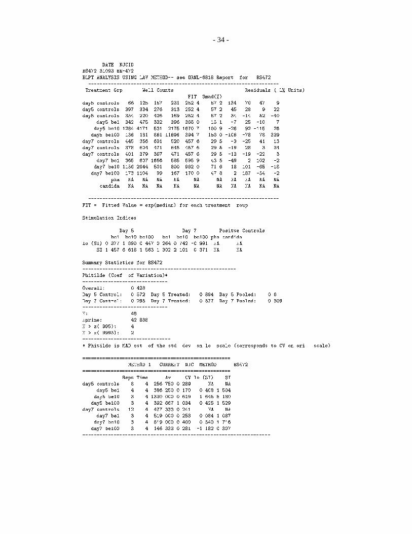
A. Detailed Report For LPT Data

The following page describes the data from day 5 and day 7 for the LPT. All statistics in the top

of the report are based on the outlier resistant approach described in Section 2.2. The results

based on the method currently in use at NJC are listed at the bottom of the report.

The left hand side of the top panel describes the treatment groups and lists the observed well

counts. Column 6 gives the fitted value obtained using the LAV method. Smad is computed

using Equations 4 (see below). The residuals rounded to the the nearest logarithmic percent

units (L%) are obtained as

Residual(L%) = 100�count

f it

For example, day 5 control well 4: 100*log(231/252.4) = -9 L%.

The LAV estimates of the log(SI)s from Equations 3 and the corresponding SIs are listed

in the second panel. Since this report was originally set up for ORISE data where positive

controls are counted on day 5, and NJC runs their positive controls on day 3, we have not

reported theses results.All LPTs in this report showed an adequate response to ConA and

PHA

The estimates of the coefficient of variation (φ) are listed near the middle of the page and

were calculated as describe in Section A.2 of ORNL-6818. A separate estimate is calculated

for the control wells and the treated wells on days 5 and 7. These same numbers are listed in

column 7 of the top panel in L% units (i.e. they have been multiplied by 100). Pooled estimates

are calculated for day 5, day 7, and overall.

- 34 -

DATE NJCID

BS472 31093 BE-472

BLPT ANALYSIS USING LAV METHOD-- see ORNL-6818 Report for BS472

-------------------------------------------------------------------

Treatment Grp Well Counts Residuals ( L% Units)

FIT Smad(%)

day5 controls 66 125 157 231 252.4 57.2 -134 -70 -47 -9

day5 controls 397 334 276 313 252.4 57.2 45 28 9 22

day5 controls 354 220 426 169 252.4 57.2 34 -14 52 -40

day5 be1 342 475 332 396 368.0 15.1 -7 25 -10 7

day5 be10 1284 4171 531 2175 1670.7 100.9 -26 92 -115 26

day5 be100 136 181 861 11696 394.7 158.0 -106 -78 78 339

day7 controls 445 356 691 520 457.6 29.5 -3 -25 41 13

day7 controls 378 604 471 645 457.6 29.5 -19 28 3 34

day7 controls 401 379 367 471 457.6 29.5 -13 -19 -22 3

day7 be1 365 607 1656 585 595.9 43.5 -49 2 102 -2

day7 be10 1156 2644 501 800 962.0 71.6 18 101 -65 -18

day7 be100 173 1104 99 167 170.0 47.8 2 187 -54 -2

pha NA NA NA NA NA NA NA NA NA NA

candida NA NA NA NA NA NA NA NA NA NA

-------------------------------------------------------------------

FIT = Fitted Value = exp(median) for each treatment group

Stimulation Indices

Day 5 Day 7 Positve Controls

be1 be10 be100 be1 be10 be100 pha candida

log(SI) 0.377 1.890 0.447 0.264 0.742 -0.991 NA NA

SI 1.457 6.618 1.563 1.302 2.101 0.371 NA NA

Summary Statistics for BS472

------------------------------------------------------

Phitilde (Coef. of Variation)*

------------------------------

Overall: 0.428

Day 5 Control: 0.572 Day 5 Treated: 0.894 Day 5 Pooled: 0.6

Day 7 Control: 0.295 Day 7 Treated: 0.577 Day 7 Pooled: 0.309

------------------------------

N: 48

Nprime: 42.888

N > z(.995): 4

N > z(.9995): 2

-------------------------------

* Phitilde is MAD est. of the std. dev. on log scale (corresponds to CV on orig. scale)

====================================================

METHOD 1 - CURRENT NJC METHOD BS472

====================================================

Reps Time Avg CV log(SI) SI

day5 controls 8 4 256.750 0.289 NA NA

day5 be1 4 4 386.250 0.170 0.408 1.504

day5 be10 3 4 1330.000 0.619 1.645 5.180

day5 be100 3 4 392.667 1.034 0.425 1.529

day7 controls 12 4 477.333 0.241 NA NA

day7 be1 3 4 519.000 0.258 0.084 1.087

day7 be10 3 4 819.000 0.400 0.540 1.716

day7 be100 3 4 146.333 0.281 -1.182 0.307

------------------------------------------------------------------

- 35 -

ORNL/TM-13338

INTERNAL DISTRIBUTION

1. D. E. Conrad2. T. S. Darland3. D. J. Downing

4–8. E. L. Frome9. C. E. Oliver

10–14. S. A. Raby15. D. E. Reichle16. P. S. Rohwer

17–21. M. Leuze22. R. F. Sincovec23. Central Research Library24. K-25 Applied Technology Library

25–26. Laboratory Records Dep.27. Laboratory Records – RC28. Patent Office29. Y-12 Technical Library

EXTERNAL DISTRIBUTION

30. B. P. Barna, Cleveland Clinic Foundation, Immunopathology, One Clinic Center, 9500Euclid Avenue, Cleveland, OH 44195-5131

31. D. L. Cragle, Medical Division, Oak Ridge Institute for Science and Education, P. O. Box117, Oak Ridge, TN 37831

32. S. P. Colyer, Medical Division, Oak Ridge Institute for Science and Education, P. O. Box117, Oak Ridge, TN 37831

33. G. R. Gebus, Occupational Medicine, EH-61, U. S. Department of Energy, 19901 Ger-mantown Road, Germantown, MD 20874

34. R. Harbek, National Jewish Center for Immunology and Respiratory Medicine, 1400Jackson Street, Denver, CO 80206

35. R. W. Hornung, National Institute for Occupational Safety and Health, 4676 ColumbiaParkway, Cincinnati, OH 45226-1998

36. K. Kreiss, Division of Respiratory Disease Studies, National Institute for OccupationalSafety and Health, 1095 Willowdale Rd, MS 234, Morgantown, WV 26505-2845

37. L. G. Littlefield, Medical Division, Oak Ridge Institute for Science and Education, P. O.Box 117, Oak Ridge, TN 37831

38. T. Markham, Brush Wellman Inc., 1200 Hanna Building, Cleveland, OH 44115

39. F. Miller, Department of Pathlogy, SUNY Stony Brook, T-140, HSC, Stony Brook, NewYork 11794-8691

40. M. A. Montopoli, Occupational Medicine, EH-61 CC 270, U. S. Department of Energy,19901 Germantown Road, Germantown, MD 20874

41. M. M. Mroz, OccupationalEnvironmental Medicine Division, National Jewish Center forImmunology and Respiratory Medicine, 1400 Jackson Street, Denver, CO 80206

42. L. S. Newman, OccupationalEnvironmental Medicine Division, National Jewish Centerfor Immunology and Respiratory Medicine, 1400 Jackson Street, Denver, CO 80206

- 36 -

43. M. D. Rossman, Hospital of the University of Pennsylvania, 812 E. Gates Building, 3400Spruce Street, Philadelphia, PA 19104

44. P. Seligman, Environmental Safety and Health, U. S. Department of Energy, 19901 Ger-mantown Road, Germantown, MD 20874

45. Y. Shim,Epidemiology and Health Surveillance, EH-62 CC 270, U. S. Department ofEnergy, 19901 Germantown Road, Germantown, MD 20874

46. H. Stockwell,Epidemiology and Health Surveillance, EH-62 CC 270, U. S. Departmentof Energy, 19901 Germantown Road, Germantown, MD 20874

47. P. F. Wambach, Occupational Medicine, EH-61 CC 270, U. S. Department of Energy,19901 Germantown Road, Germantown, MD 20874

48. Office of Assistant Manager for Energy Research and Development, DOE-ORO, P.O. Box2008, Oak Ridge, TN 37831-6269

49–50. Office of Scientific and Technical Information, P.O. Box 62, Oak Ridge, TN 37830

Documents

537KB - Computer Science and Mathematics Division - Oak