arX

iv:0

903.

2361

v7 [

mat

h.O

C]

21

Jun

2013

AdaptiveObservers andParameterEstimation for aClass

of SystemsNonlinear in theParameters

Ivan Y. Tyukin a Erik Steur b Henk Nijmeijer c Cees van Leeuwen b

aDept. of Mathematics, University of Leicester, Leicester, LE1 7RH, UK (Tel: +44-116-252-5106; I.Tyukin@le.ac.uk)

bLaboratory for Perceptual Dynamics, KU Leuven, Tiensestraat 102, 3000 Leuven, Belgium (erik.steur@ppw.kuleuven.be,cees.vanleeuwen@ppw.kuleuven.be)

cDept. of Mechanical Engineering, Eindhoven University of Technology, P.O. Box 513 5600 MB, Eindhoven, TheNetherlands, (h.nijmeijer@tue.nl)

Abstract

We consider the problem of asymptotic reconstruction of the state and parameter values in systems of ordinary differentialequations. A solution to this problem is proposed for a class of systems of which the unknowns are allowed to be nonlinearlyparameterized functions of state and time. Reconstruction of state and parameter values is based on the concepts of weaklyattracting sets and non-uniform convergence and is subjected to persistency of excitation conditions. In the absence ofnonlinear parametrization the resulting observers reduce to standard estimation schemes. In this respect, the proposed methodconstitutes a generalization of the conventional canonical adaptive observer design.

Key words: Adaptive observers, nonlinear parametrization, weakly attracting sets

1 Introduction

We consider observer-based methods for state and pa-rameter estimation in nonlinear dynamical systems.These methods are effective as long as the original sys-tem has, or can be transformed into, one of the canoni-cal adaptive observer forms [5], [25], [6]. Their commoncharacteristic is linearity in the unknown parameters.For this class of systems, subject to persistency of exci-tation conditions, reconstruction of state and parametervectors can be achieved exponentially fast.

There are systems, however, in which the unknown pa-rameters enter the model nonlinearly. These systemsconstitute a remarkably wide class including models inchemical kinetics [13], [4], biology and neuroscience [18].Whereas the problem of state estimation can be solvedfor a large class of nonlinearly parameterized systems[28], observer-based parameter reconstruction is oftenconfined to systems with monotone [39], [22] or one-to-one parameterizations [14], [15], [16], [12].

⋆ This paper was not presented at any IFAC meeting. Ceesvan Leeuwen is supported by an Odysseus grant from theFlemish Science Organization FWO. Corresponding authorI. Yu. Tyukin. Tel. +44-116-2525106.

Several authors have recently advanced strategies forovercoming these limitations. In [19], combining intervalanalysis with multiple shooting methods is proposed totackle the state and parameter reconstruction problem.Another interesting approach is presented in [1]: the orig-inal continuous-time model is replaced with a discrete-time approximation. Measured variables are then con-sidered as known functions of unknown parameters andinitial conditions, of which the estimates can be foundby off-line nonlinear optimization routines (see also [36],[2] where optimization techniques with moving horizonare discussed). These approaches offer obvious advan-tages, e.g. the availability of a vast library of numeri-cal methods for solving general nonlinear optimizationproblems. Nevertheless, these methods run into restric-tions too. Exhaustive search for a global minimum maybecome intractable for dimensions higher than 1 or 2. Onthe other hand, if conventional polynomial-complexityalgorithms are used then the possibility arises that thealgorithm will converge to a local minimum.

In this paper we explore further possibilities of develop-ing adaptive observers for systems which are both lin-early and nonlinearly parameterized. The parametriza-tion is not required to be invertible or monotone. Our ap-proach combines the advantages of the existing schemes,

Preprint submitted to Automatica May 28, 2018

in being capable of ensuring exponentially fast conver-gence with the flexibility of explorative behavior, a be-havior inherent to algorithms for solving genuine non-linear optimization problems. Inference of the values ofstate and a part of the parameter vector of these sys-tems is achieved by employing exponentially fast con-verging estimators. Estimation of the values of the re-maining parameters is based on an explorative searchprocedure. Since exploration is restricted to a subset ofthe unknown parameters, the proposed strategy reducesthe overall computational costs, as compared to whenfull-scale search-based optimization had been invoked.

The resulting observer can be imagined as a system com-prising of an exponentially stable part coupled with anexplorative one. Systems of this type have previouslybeen used in adaptive control [34], [17], [29], [30]. Herewe demonstrate that these classical ideas can be ap-plied to the problem of adaptive observer design for sys-tems which are nonlinearly dependent on parameters.We show that, subject to a condition of persistent exci-tation, it is possible to reconstruct state and parametersof a reasonably broad subclass of these systems.

The paper is organized as follows. Notational agreementsare introduced in Section 2. Section 3 provides the for-mal statement of the problem, Sections 4, 5 containmainresults of the article, Section 6 discusses possible gener-alizations, Section 7 contains illustrative examples, andSection 8 concludes the paper. Proofs of auxiliary resultsare presented in the Appendix.

2 Notation

The following notational conventions are used through-out the paper:

• R denotes the set of real numbers,R>a = x ∈ R | x >a, and R≥a = x ∈ R | x ≥ a;

• Z denotes the set of integers, and N stands for the setof positive integers;

• the Euclidean norm of x ∈ Rn is denoted by ‖x‖,

‖x‖2 = xTx, where T stands for transposition;• the space of n×nmatrices with real entries is denotedbyRn×n; letP ∈ R

n×n, thenP > 0 (P ≥ 0) indicatesthat P is symmetric and positive (semi-)definite; Indenotes the n× n identity matrix.

• by Ln∞[t0, T ], t0 ∈ R, T ∈ R, T ≥ t0 we denote

the space of all functions f : [t0, T ] → Rn such

that ‖f‖∞,[t0,T ] = ess sup‖f(t)‖, t ∈ [t0, T ] < ∞;‖f‖∞,[t0,T ] stands for the Ln

∞[t0, T ] norm of f(t); ifthe function f is defined on a set larger than [t0, T ]then notation ‖f‖∞,[t0,T ] applies to the restriction off on [t0, T ];

• Cr denotes the space of continuous functions that areat least r times differentiable;

• LetA be a subset ofRn, then for all x ∈ Rn, we define

dist(A,x) = infq∈A ‖x− q‖;

• A solution of x = f(t,x, θ, u(t)), f : R×Rn ×R

m ×R → R

n, θ ∈ Rm, u : R → R passing through x0 ∈

Rn at t = t0 is denoted by x(t, t0,x0, θ, [u]). In cases

when u and/or θ, x0, t0 are clearly determined by thecontext a more compact notation, x(t, t0,x0, θ) (orx(t, t0,x0), x(t), x respectively), is used.

• The symbol K denotes the class of all strictly increas-ing continuous functions κ : R≥0 → R≥0 such thatκ(0) = 0; the symbol K∞ denotes the class of all func-tions κ ∈ K such that lims→∞ κ(s) = ∞.

• Let ǫ ∈ R≥0, then ‖x‖ǫ stands for: ‖x‖− ǫ if ‖x‖ > ǫ,and 0 otherwise.

• Finally, for λ ∈ Rp and θ ∈ R

m, the notation (λ, θ)stands for col(λ1, . . . , λp, θ1, . . . , θm).

3 Preliminaries and Problem formulation

3.1 Adaptive observer canonical form

Throughout the paper we will focus exclusively on theclass of systems that are forward-complete:

Definition 1 Let Lu[t0,∞] be a subspace of L∞[t0,∞].A single-input single-output system described by x =f(t,x, u(t)), f : R × R

n × R → Rn, y = h(t,x), h :

R×Rn → R, u ∈ Lu[t0,∞], where u is the input, and y

is the output, is called forward-complete (with respect toLu) iff for any t0 ∈ R, x0 ∈ R

n, and u ∈ Lu[t0,∞] thesolution x(t, t0,x0, [u]) exists and is defined for all t ≥ t0.

Let Lu[t0,∞] = L∞[t0,∞] ∩ C0[t0,∞], and consider aforward-complete single-input single-output system; letx ∈ R

n be its state, y : R → R be the measured output,and u : R → R, u ∈ Lu be the input. We recall that asystem is in the adaptive observer canonical form if it isgoverned by the following set of equations

x = Ax+BφT (t, y)θ + g(t, y, u(t))

y = CTx, x(t0) = x0, x0 ∈ Rn,

(1)

where A =

(

aIn−1

0

)

, a ∈ Rn, B ∈ R

n, C ∈ Rn, B =

col(1, b1, . . . , bn−1), C = col(1, 0, . . . , 0), the functionsφ : R × R → R

m, g : R × R × R → Rn, φ,g ∈ C0

are known, and θ ∈ Rm is the vector of the unknown

parameters. The triplet A,B,C is supposed to satisfy

P(A+ ℓCT ) + (A+ ℓCT )TP ≤ −Q

PB = C.(2)

for some ℓ ∈ Rn and P > 0, Q > 0. Although condition

(2) may appear restrictive, it has been shown in [26]that subject to the very natural constraint that the pairA,C is observable, there is a time-varying parameter-dependent coordinate transformation such that in new

2

coordinates the system is still of the form (1) and satisfiescondition (2). If requirement (2) holds then the system

˙x =Ax+ ℓ (CT x− y(t)) +BφT (t, y(t))θ

+ g(t, y(t), u(t))

˙θ =− γ(CT x− y(t))φ(t, y(t)), γ ∈ R>0,

(3)

where x(t) ∈ Rn, θ(t) ∈ R

m, is an adaptive observer for(1) (cf. [25], [5]) provided that the restriction ofφ(·, y(·))on R≥t0 is persistently exciting:

Definition 2 A function β : R≥t0 → Rm is said to be

persistently exciting if there exist L, µ ∈ R>0:

∫ t+L

t β(τ)βT (τ)dτ ≥ µIm, ∀ t ≥ t0. (4)

The fact that (3) is an adaptive observer for (1) is basedon a well-known result on the exponential stability ofthe following class of linear time-varying systems 1

e = A(t)e, A(t) =

(

A+ ℓCT BβT (t)

−β(t)CT 0

)

. (5)

The result is provided in Theorem 3 below (see e.g. [23]for a proof).

Theorem 3 Consider system (5). Suppose that condi-tion (2) holds for certain ℓ ∈ R

n, P > 0, Q > 0, thefunction β(t) is persistently exciting, and

∃ M ∈ R>0 : max‖β(t)‖, ‖β(t)‖ ≤ M ∀ t ≥ t0. (6)

Let Φ(t, t0), Φ(t0, t0) = In+m, be the fundamental solu-tion matrix of (5). Then there exist ρ,D ∈ R>0 such that‖Φ(t2, t1)p‖ ≤ De−ρ(t2−t1)‖p‖ for all t2 ≥ t1 ≥ t0 andp ∈ R

n+m.

The parameters ρ and D can be expressed explicitly asfunctions ofM , µ, L, andA,B,C, ℓ [23]. By letting e =

col(x−x, θ−θ) and taking (1), (3) into account one canconfirm that the system-observer equations are of form(5). Thus, subject to persistency of excitation of the re-

striction of φT (·, y(·)) on R≥t0 , limt→∞ x(t, t0, x0, θ0)−x(t, t0,x0, θ) = 0, limt→∞ θ(t, t0, x0, θ0) = θ along thesolutions of (1), (3), and the convergence is exponential.The problem, however, is that if some parameters enterthe equations nonlinearly then this creates an obstaclefor the explicit use of Theorem 3 and, consequently, ob-server (3). In the next sections we present and analyze aclass of systems nonlinear in the parameters which canbe thought of as an immediate generalization of (1).

1 In the context of adaptive observer design for (1) the func-tion β in (5) is defined as β(t) = φ(t, y(t)), t ≥ t0.

3.2 Systems considered in this article

We begin with the following class of forward-completesingle-input-single-output nonlinear systems:

x = Ax+BϕT (t,λ, y)θ + g(t,λ, y, u(t)) + ξ(t),

y = CTx, x(t0) = x0, x0 ∈ Rn,

(7)

where A ∈ Rn×n, and B,C ∈ R

n are defined as in (1);ϕ : R×R

p ×R → Rm, g : R×R

p ×R×R → Rn, are

known continuous functions, λ = col(λ1, . . . , λp) ∈ Rp,

θ = col(θ1, . . . , θm) ∈ Rm are unknown parameters, and

u ∈ Lu ∩ C1, is the input. We assume that the values ofλ, θ belong to the hypercubes Ωλ ⊂ R

p, Ωθ ⊂ Rm with

known bounds: θi ∈ [θi,min, θi,max], λj ∈ [λj,min, λj,max],and that y(t) ∈ Dy, u(t) ∈ Du, Dy,Du ⊂ R for t ≥ t0.

In (7), x = col (x1, x2, . . . , xn) ∈ Rn is the state vector, y

is the measured output, the input u is a known function,and ξ ∈ C0 : R → R

n is an unknown yet boundedcontinuous function:

∃ ∆ξ ∈ R≥0 : ‖ξ(t)‖ ≤ ∆ξ ∀ t, (8)

representing some unmodeled dynamics (e.g. noise). Thesystem’s state x is not measured; only the values of theinput u(t) and the output y(t) = x1(t), t ≥ t0 in (7) areaccessible over any time interval [t0, t] that belongs tothe history of the system.

For the time being we suppose that matrixA and vectorsB,C in (7) satisfy Assumption 3.1 below.

Assumption 3.1 The triple A,B,C is known, andthere exist (and are known) a vector ℓ and matricesP,Q > 0 such that condition (2) holds.

Note that Assumption 3.1 implies that the vector B =col(1, b1, . . . , bn−1) in (7) is such that the polynomialsn−1+ b1s

n−2+ · · ·+ bn−1 is Hurwitz. At first, Assump-tion 3.1 may seem restrictive. In Section 6 we lift thisrestriction by showing that the results presented for (7)can be generalized to systems

x = Ax+Ψ(t,λ, y)θ + g(t,λ, y, u(t)) + ξ(t),

y = CTx, C = col (1, 0, . . . , 0) ,(9)

in which the matrix A ∈ Rn×n may be unknown but it

is known that the pair A,C is observable, the functionΨ : R × R

p × R → Rn×m, Ψ ∈ C1, is Lipschitz in

λ, and g(·,λ, y(·), u(·)), g(·,λ, y(·), u(·)), Ψ(·,λ, y(·)),Ψ(·,λ, y(·)) are bounded for all λ ∈ Ωλ on [t0,∞).

With regards to the functions ϕ and g in (7) the follow-ing additional technical assumptions are made:

3

Table 1Examples of physical systems in the form of (7), (9)

Physical system Model Possible parametrization: θ, λ, A, B, ϕ, Ψ, g

1. Reactant dy-namics in a reac-tor [35]

x = FV(x0 − x)− krefe

−ER

(

1T (t)

−1

Tref

)

x,

y = x

System (7): θ = col(

FVx0,−

FV,−krefe

ERTref

)

, λ = −ER,

A = 0, B = 1, ϕ(t, λ, y) = col(

1, y, eλ 1

T(t) y)

, g = 0

2. Magnetic bear-ings [21]

x+ J−1d(t) = b(

q22(I2,a,x)

(x+a)2−

q21(I1,a,x)

(x−a)2

)

y = x, |x| < a− ε, a, ε ∈ R>0,

d, d are bounded

System (7): θ = col(

−J−1, b)

, A =

0 1

0 0

, B =

0

1

,

λ = a, ϕ(t, λ, y) = col(

d(t),q22(I2,λ,y)

(y+λ)2−

q21(I1,λ,y)

(y−λ)2

)

, g = 0

3. Action poten-tials in a cell [37]

x1 = − x1τm

+Af

τmtanh

(

σf

Afx1

)

− x2τm

x2 = −x2τs

+ σs

τsx1

y = x1

System (9): θ = col(

− 1τm

,Af

τm, σs

τs

)

, λ =σf

Af, A =

0 − 1τm

0 − 1τs

, Ψ(t, λ, y) =

y tanh(λy) 0

0 0 y

, g = 0

Assumption 3.2 The functions ϕ(·,λ, ·), g(·,λ, ·, ·) in(7) are bounded and differentiable in R≥t0 × Dy andR≥t0 × Dy × Du respectively, and Lipschitz in λ. Thatis, there exist Dϕ, Dg, Bϕ, Bg ∈ R≥0 such that for allt ∈ R≥t0 , y ∈ Dy, u ∈ Du, λ

′,λ′′ ∈ Ωλ

‖ϕ(t,λ′, y)−ϕ(t,λ′′, y)‖ ≤ Dϕ‖λ′ − λ′′‖,‖g(t,λ′, y, u)− g(t,λ′′, y, u)‖ ≤ Dg‖λ′ − λ′′‖, (10)

‖ϕ(t,λ, y)‖ ≤ Bϕ, ‖g(t,λ, y, u)‖ ≤ Bg. (11)

Furthermore, there exist Mϕ,Mg ∈ R≥0 such that

∣

∣

∣

∂ϕ(t,λ,y)∂y y + ∂ϕ(t,λ,y)

∂t

∣

∣

∣ ≤ Mϕ , (12)∣

∣

∣

∂g(t,λ,y,u)∂y y + ∂g(t,λ,y,u)

∂u u+ ∂g(t,λ,y,u)∂t

∣

∣

∣≤ Mg

for all λ ∈ Ωλ, t ≥ t0 along the solutions of (7).

Conditions (10), (11) often hold naturally in the contextof modeling and identification; they may, however, im-pose limitations in the framework of controller design.As for condition (12), the first inequality is a version of(6) that is essential for uniform exponential convergenceof solutions to the origin of (5) [23]. The second inequal-ity in (12) is a technical condition. Although this lattercondition may look somewhat restrictive, it may be re-laxed if g(t,λ, y, u(t)) is expressed as g(t,λ, y, u(t)) =g1(t, y, u(t)) + g2(t,λ, y, u(t)). In this case we would re-quire that (11), (12) hold for g2.

A non-exhaustive list of systems that are relevant in en-gineering applications and are governed by (7) or (9)includes bio-/ chemical reactors [7,35], nonlinear satu-rated magnetic circuits [32], magnetic bearings [21], tire-road interaction, and dynamics of live cells [37]. A fewexamples from this list are provided in Table 1. The firstmodel, if described by (7), trivially satisfies Assump-tion 3.1; it also satisfies Assumption 3.2 if T is bounded,differentiable, separated away from zero, and y, T are

bounded. In the second model the pair A, C is observ-able, and ϕ, ϕ are bounded if y, magnetic fluxes, ex-pressed by q1,q2, and q1, q2 are bounded. This is achiev-able via external controls [21], at least for small para-metric mismatches and d. In the third model the pairA, C is observable, and boundedness of y, y, Ψ, Ψ isconsistent with the physics of the system.

3.3 Problem formulation

Before we proceed with a formal problem statement, sev-eral points related to parametrization of (7), (9) need tobe discussed. First, note that different definitions of sys-tems (7), (9) may correspond the same physical model.For example, functions ϕ and g and parameters θ,λ forthe first model in Table 1 may also be defined as:

ϕ(t,λ, y) = col(

1, y, eλ11

T (t)+λ2y

)

, g = 0, (13)

θ = col(

FV x0,−F

V ,−kref)

, λ = col(

−ER , E

RTref

)

, or

ϕ(t,λ, y) = col (1, y) , g(t,λ, y, u(t)) = −eλ11

T (t)+λ2y,(14)

with θ = col(

FV x0,−F

V

)

, λ = col(

− ln(kref )ER , ln(kref )E

RTref

)

.

It is clear that if parametrization (13) is chosen thenidentical outputs y(t) will be observed for infinitelymany combinations of parameters θ3, λ2. Models ofthis type are referred to as unidentifiable [11] (see also[9], [10]). Dealing with unidentifiable models imposestechnical difficulties. We will therefore assume thatparametrizations which are obviously unidentifiable areavoided, if possible. As for the remaining alternativeparametrizations, we assume that preference is given tothose in which the dimension of λ is minimal, i.e. theparametrization in the first row in Table 1 is preferableto (14).

Second, as far as identifiability is concerned, inferringtrue values of θ, λ from output observations, y(t), is not

4

always possible, even if the system is linearly parameter-ized and no unmodeled dynamics are present. Consider

x = Ax+

(

1

1

)

θ +

(

0

1

)

λ, A =

(

−a1 1

−a2 0

)

y = x1, a1, a2 ∈ R>0.

(15)

Let x(t, θ, λ,x0) and x(t, θ′, λ′,x′0) be two solutions of

(15) corresponding to different parameter values and ini-tial conditions, and let e = col(e1, e2) = x(t, θ, λ,x0) −x(t, θ′, λ′,x′

0). Picking e2(t0) = −θ + θ′, e1(t0) = 0 en-sures that e1(t) = 0 for all t ≥ t0 if θ − θ′ + λ − λ′ = 0.Another, albeit nonlinearly parameterized, example is

x = −x+ θ + [sin2(λ+ t) + x2 + 1]−1, y = x. (16)

In this case x(t, θ, λ, x0) = x(t, θ, λ′, x0) for all t ≥ t0 ifλ′ = λ+ kπ, k ∈ Z, θ′ = θ.

In order to account for possible non-unique parametriza-tion, for each pair θ,λ we introduce two sets: E0(λ, θ)and E(λ, θ). The set E0(λ, θ):

E0(λ, θ) = (λ′, θ′), λ′ ∈ Rp, θ′ ∈ R

m|η0(t,λ, θ,λ

′, θ′) = 0, ∀ t ≥ t0,(17)

η0(t,λ, θ,λ′, θ′) =

B(ϕT (t,λ, y(t))θ −ϕT (t,λ′, y(t))θ′) +g(t,λ′, y(t), u(t))− g(t,λ, y(t), u(t))

contains all parametrizations of (7) that are indis-tinguishable from observations of x(t) for the giveny(·), u(·), θ, λ at ξ(t) ≡ 0. That is, if x(t, θ,λ,x0) −x(t, θ′,λ′,x0) = 0 for all t ≥ t0 then (λ′, θ′) ∈ E0(λ, θ).For system (15) the set E0(λ, θ) contains just one ele-ment, (λ, θ). The set E0(λ, θ), however, is not finite forsystem (16) and for parametrization (13) of the firstmodel in Table 1.

The second set, E(λ, θ), is defined as:

E(λ, θ) = (λ′, θ′),λ′ ∈ Rp, θ′ ∈ R

m | ∃ p(θ,λ, θ′,λ′)

∈ Rn−1 : CT eΛ(t−t0)p+ η(t, θ,λ, θ′,λ′) = 0 ∀ t ≥ t0,

(18)

where C ∈ Rn−1, C = col(1, 0, . . . , 0),

η(t,λ, θ,λ′, θ′) = ϕ(t,λ, y(t))Tθ −ϕ(t,λ′, y(t))Tθ′ +g1(t,λ, y(t), u(t))− g1(t,λ

′, y(t), u(t)) + q(t,λ,λ′) (19)

and q(t,λ,λ′) = CT z(t,λ,λ′):

z=Λz+G(g(t,λ, y(t), u(t))− g(t,λ′, y(t), u(t))),

Λ=

(

−bIn−2

0

)

, G =(

−b In−1

)

(20)

z(t0) = 0, b = col (b1, . . . , bn−1) .

If ξ(t) ≡ 0 then the set E(λ, θ) contains all indistinguish-able parametrizations of (7) for the given y(·), u(·), θ,λ (see Lemma 12 in Section 5), and E0(λ, θ) ⊆ E(λ, θ).Note that if dim(x) = 2 then Λ = −b1, G = (−b1 1); ifdim(x) = 1 we set E(λ, θ) = E0(λ, θ). For system (15),E(λ, θ) = (λ′, θ′), λ ∈ R, θ ∈ R| θ − θ′ + λ − λ′ = 0.Note that if g(t,λ, y(t), u(t)) = Bg(t,λ, y(t), u(t)), B =col(1, b1, . . . , bn−1), then q(t,λ,λ′) ≡ 0 for all t ≥ t0in (19). The introduction of sets E0(λ, θ), E(λ, θ) doesnot, of course, resolve identifiability issues. It helps, how-ever, to specify constraints on the nonlinearities in (7)for which the parameter reconstruction, up to E0, E , canbe achieved.

Since this is desirable from an implementation point ofview, we will seek for a recursive procedure taking thevalues y(t), u(t) as inputs and producing the estimates

x(t), θ(t), λ(t) of x(t,λ, θ,x0, [u]), θ, and λ, respec-tively, as outputs. Note that since we allow for non-identifiable configurations, estimation of parameters θ,λ is possible only up to the set E(λ, θ). We will, there-fore, be looking for an auxiliary system, i.e. an adaptiveobserver: q = f(t, y, u(t),q), f : R×R×R×R

q → Rq,

q(t0) = q0, q ∈ Rq, and functions hθ : R

q → Rm,

hλ : Rq → Rp, hx : Rq → R

n such that for the givent0, appropriately chosen q0, known functions r1, r2 ∈ K,and all admissible λ, θ,x0 the following requirementshold for the observer:

lim supt→∞

‖hx(q(t,q0))− x(t,λ, θ,x0)‖ ≤ r1(∆ξ) (21)

lim supt→∞

dist

((

hλ(q(t,q0))

hθ(q(t,q0))

)

, E(λ, θ))

≤ r2(∆ξ),

where ∆ξ is defined in (8).

4 Main result

In this section we introduce an observer for (7) and showthat asymptotic reconstruction of state and parametersof (7) is achievable (up to the set E(λ, θ)), subject tosome persistency of excitation conditions.

4.1 Observer definition

Following the general ideas of [40] with regards to thetreatment of uncertain systems with general nonlinear

5

ss 24

s1

l1, max

s3

l 2, max

l 2, min

l1, min

l( )t

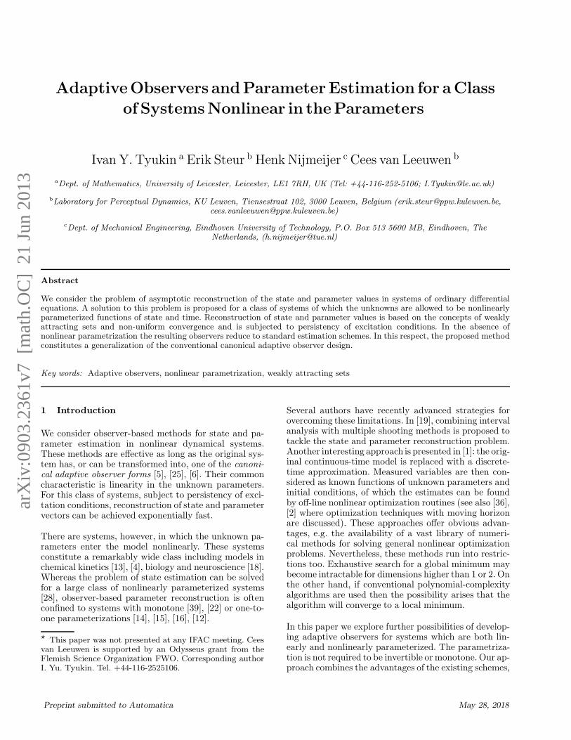
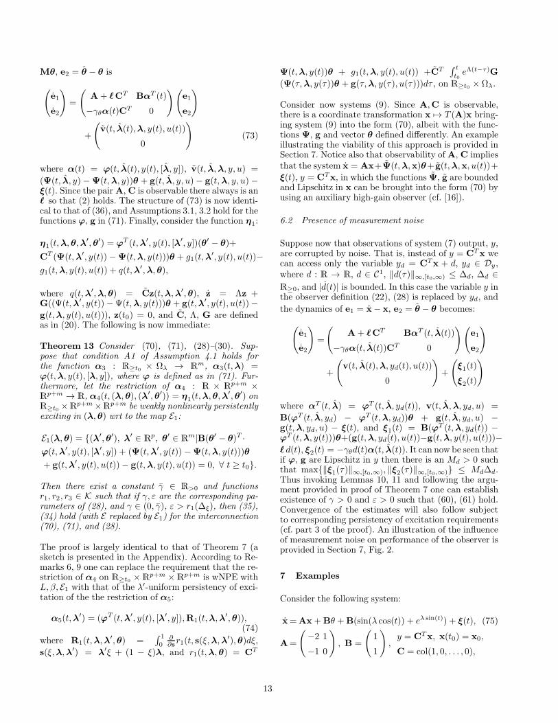
Figure 1.Top panel: general structure of the observer.Bottompanel: phase curves of system (25).

parametrization, we propose that an asymptotically con-verging observer for (7) consists of two coupled subsys-tems, Sa and Sw (see Fig. 1). The role of subsystem Sa

is to provide estimates of state and parameters θ of (7),and the role of subsystem Sw is to search the values ofparameters λ.

The dynamics of subsystem Sa is defined as follows:

Sa :

˙x =Ax+ ℓ (CT x− y(t)) +BϕT (t, λ(t), y(t))θ

+ g(t, λ(t), y(t), u(t))

˙θ =− γθ(C

T x− y(t))ϕ(t, λ(t), y(t)),

y =CT x, x(t0) ∈ Rn, θ(t0) ∈ R

m, γθ ∈ R>0

(22)

The variable θ = col(θ1, · · · , θm) in (22) is an estimate

of θ, and λ = col(λ1, . . . , λp) is an estimate of λ. For the

time being we suppose that λ is a continuous function oft. The matrixA and vectorsB,C in (22) are identical tothose in (7), and the vector ℓ in (22) satisfiesAssumption3.1. If the values of λ would be known then substitutionλ = λ reduces system (22) to (3), and conditions forasymptotic reconstruction of state and parameter valuesof (7) follow from Theorem 3. The values of λ, however,are unknown and therefore a procedure for estimatingthe values of λ is needed.

Regarding the definition of Sw, we propose that the val-

ues of λ(t) result from an explorative search in the do-main Ωλ of the admissible values for λ. The explorationcan be realized by movements along the solutions of acertain class of dynamical systems. Let us, for instance,consider systems governed by the following equations

s = f(s), s(t0) = s0, λ = β(s) (23)

where f : Rnp → Rnp , β : Rnp → R

p are continuous,and let Ωs be the ω-limit set 2 of s0. In addition, supposethat the following properties hold:

P1) the functions f , β in (23) are Lipschitz;P2) the vector s0 is such that the solution s(t, s0) is

bounded for all t ≥ t0;P3) the image of Ωs under β contains Ωλ: for every

λ ∈ Ωλ there is an s ∈ Ωs such that β(s) = λ.

Properties P1 and P2 are technical requirements ensur-

ing that the derivative of λ, as a function of t, is boundedand has a bounded growth rate. Property P3, however,is essential. It implies that the projection β(s(·, s0)) ofthe trajectory s(·, s0) onto Ωλ is dense and recurring inΩλ:

∀ λ ∈ Ωλ, ∀ ε ∈ R>0, ∀ t ≥ t0

∃ t′ > t : ‖λ− β(s(t′, s0))‖ < ε.(24)

Indeed, let λ′ be an element from Ωλ. Then accordingto P3 there is an s′ ∈ Ωs: β(s

′) = λ′. Since Ωs is theω-limit set of s0, we can conclude that there is a se-quence ti, i = 1, 2, . . . , limi→∞ ti = ∞, such thatlimi→∞ s(ti, s0) = s′. Finally, using the continuity of βwe arrive at limi→∞ β(s(ti, s0)) = λ′. In other words, forany λ′ ∈ Ωλ and ε > 0 there will exist a sequence of time

instances ti : limi→∞ ti = ∞ such that ‖λ(ti)−λ′‖ < ε,and hence (24) follows. An example of a very simple sys-tem possessing a solution s(t, s0) and an output functionβ satisfying properties P1–P3 for Ωλ = [−1, 1]2 is

s1 = −√2s2, s2 =

√2s1, s3 = −s4, s4 = s3,

β(s(t, s0)) = col(s1(t), s3(t)), s0 = col (1, 0, 1, 0) .(25)

Phase curves of (25) are shown in Fig. 1, bottom panel.Projections of the initial segment of the trajectory areshown by thick lines. After evolving beyond the initialsegment, the values of β(s(t, s0)) will densely fill the set[λ1,min, λ1,max]× [λ2,min, λ2,max] = [−1, 1]2, cf. [33].

The problem with using (23) directly as an estimator forλ is that exploration of the set Ωλ continues indefinitely.For the purposes of observer design we need to ensurethat exploration of Ωλ stops once a sufficiently smallneighborhood of the set E(λ, θ) has been reached. Toenable this, the explorative subsystem must be suppliedwith an error measure. A function of ‖y(t)− y(t)‖ε is apossible candidate for such a measure. Thus we replace

the earlier definition (23) for λ with the following:

s = γσ(‖y(t)− y(t)‖ε)f(s), ε ∈ R≥0, γ ∈ R>0,

λ = β(s), s(t0) = s0,(26)

2 Recall that a point z ∈ Rnp is an ω-limit point of z0 ∈ Rnp

if there is a sequence ti, i = 1, 2, . . . , limi→∞ ti = ∞, suchthat limi→∞ s(ti, z0) = z. The set of all ω-limit points of z0is the ω-limit set of z0.

6

where σ : R≥0 → R≥0 is a bounded Lipschitz function:

∃ Dσ, Mσ ∈ R>0 :

σ(υ) ≤ Mσ, σ(υ) ≤ Dσυ ∀ υ ≥ 0(27)

such that σ(υ) > 0 for υ > 0, and σ(0) = 0.

For the sake of simplicity and without loss of general-ity, instead of dealing with general systems (26), we willfocus on a specific system of equations:

Sw :

s2j−1 = γσ(‖y(t)− y(t)‖ε) · ωj · (s2j−1 − s2j

−s2j−1(s22j−1 + s22j))

s2j = γσ(‖y(t)− y(t)‖ε) · ωj · (s2j−1 + s2j

−s2j(s22j−1 + s22j))

λj = βj(s), j = 1, . . . , p,

βj(s) = λj,min +λj,max − λj,min

2(s2j−1 + 1)

(28)

s0 = s(t0) : s22j−1(t0) + s22j(t0) = 1, (29)

where σ is a function satisfying (27). Parameters ωj ∈R>0 in (28) are supposed to be rationally-independent:

∑pj=1 ωjkj 6= 0, ∀ kj ∈ Z. (30)

Equations (28)–(30) are straightforward generalizationsfrom the example system of which the phase curves areshown in Fig. 1. If the term γσ(‖y(t) − y(t)‖ε) in theright-hand side of (28) is substituted with 1, these equa-tions satisfy the requirements P1–P3. Indeed, we can im-mediately see that in this case (s2j−1(t, s0), s2j(t, s0)) =(cos(ωj(t− t0)+ aj), sin(ωj(t− t0)+ aj)), aj ∈ R. Thusproperties P1, P2 hold. Trajectories s1(·, s0), s3(·, s0),. . . s2p−1(·, s0) evolve on a corresponding p-dimensionalinvariant torus. Since ωj are rationally-independentthese trajectories densely fill the torus (cf. [3], [33],[20]) or, alternatively, they densely fill the hypercube[−1, 1]p. This implies that Ωs, the ω-limit set of s0, isΩs = col (s1, s2, . . . , s2p) ∈ R

p| col (s1, s3, . . . , s2p−1) ∈[−1, 1]p, s2j = ±

√

1− s22j−1, j = 1, . . . , p. Noticingthat the image of Ωs under transformation β coincideswith Ωλ we conclude that P3 holds.

Concerning the structure of Sw, no additional model-dependent constraints are imposed on (28) (or, in gen-eral, on (26)), apart from the general requirements P1–P3. Model-specific nonlinearities are accounted for inthe “converging” part, Sa, of the observer producing theestimates for θ and x. The information about the val-ues of λ is transferred to the exploratory part, Sw, bymeans of ‖y(t) − y(t)‖ε. The latter variable modulatesthe speed of exploration in Ωλ along a search trajectory.

The search trajectory itself does not need to be depen-dent on the properties of g, ϕ, and neither is the struc-ture of Sw. This potential advantage of the approach,however, comes at a cost. According to (24), small neigh-borhoods of sets to which the solutions of the combinedsystem (22), (28) converge are not necessarily forwardinvariant. Hence these sets are not guaranteed to beasymptotically stable. Nevertheless, albeit in a weakersense [31], they are still attracting. We illustrate thispoint in Section 7.

4.2 Asymptotic properties of the observer

Let us now proceed with specifying those properties of(7) that can be useful for state and parameter recon-struction. Recall that (7) is a generalization of the stan-dard canonic observer form (1). According to Theorem3, one of the conditions for (3) to be an adaptive observerfor (1) is persistency of excitation of the restriction ofφ(·, y(·)) on R≥t0 . It is therefore natural to expect thatsome kind of persistency of excitation conditions mightbe needed for reconstruction of parameters θ, λ in (7)too. Two versions of these conditions will be considered,namely the notions of uniform persistency of excitation[24] and nonlinear persistency of excitation [8].

Definition 4 A function α : R≥t0 × Ωλ → Rp is λ-

Uniformly Persistently Exciting (λ-UPE with T , µ), de-noted byα(t,λ) ∈ λUPE(T, µ), if there exist T, µ ∈ R>0:

∫ t+T

t α(τ,λ)αT (τ,λ)dτ ≥ µIp, ∀ t ≥ t0, λ ∈ Ωλ.

(31)

In contrast to the conventional definitions of persistencyof excitation (cf. Definition 2), uniform persistency ofexcitation requires existence of µ, T ∈ R>0 in (31) thatare independent on λ for all λ ∈ Ωλ. This is a strongerrestriction; we will, however, require that it holds forϕ(t,λ, y(t)) (as a function of t,λ on R≥t0 × Ωλ) in (7).

Since parametrization of (7) is allowed to be nonlinear,it is natural to expect that reconstruction of model pa-rameters might require a nonlinear version of standardpersistency of excitation. Here we employ the followinggeneralization of the standard notion (cf. [8]):

Definition 5 Let E be a set-valued map defined on D ⊂R

d and associating a subset of D to every p ∈ D. Afunction α : R≥t0 × D × D → R

k is said to be weaklyNonlinearly Persistently Exciting in p wrt E (wNPE withL, β, E ), denoted byα(t,p,p′) ∈ wNPE(L, β, E), if thereexist L ∈ R>0, t1 ≥ t0, and β ∈ K∞:

∀ t ≥ t1, p,p′ ∈ D ∃ t′ ∈ [t, t+ L] :

‖α(t′,p,p′)‖ ≥ β (dist(E(p),p′)) .(32)

7

If the set E(p) contains just one element, p, then theinequality in (32) reduces to ‖α(t′,p,p′)‖ ≥ β(‖p−p′‖).Taking the above notions into account we formulate themain technical assumption on the nonlinearities in (7):

Assumption 4.1 The functions ϕ, g in the right-handside of (7) are such that

A1) the restriction of the function α1 : R×Rp → R

m,α1(t,λ) = ϕ(t,λ, y(t)) onR≥t0×Ωλ is λ-UPE withT, µ;

A2) the restriction of α2 : R × Rp+m × R

p+m → R,α2(t, (λ, θ), (λ

′, θ′)) = η(t,λ, θ,λ′, θ′), where η(·)is defined in (19), onR≥t0×R

p+m×Rp+m is weakly

nonlinearly persistently exciting in (λ, θ) wrt to themap E(λ, θ) determined by (18).

Remark 6 Checking that condition A1 holds isstraightforward if e.g. ϕ(t,λ, y(t)) is periodic in t. Re-garding condition A2, we note that, according to (19),η(t,λ, θ,λ′, θ′) can be expressed as η(t,λ, θ,λ′, θ′) =r(t,λ, θ)− r(t,λ′, θ) +ϕ(t,λ′, y(t))T (θ − θ′), where

r(t,λ, θ) = ϕ(t,λ, y(t))Tθ + g1(t,λ, y(t), u(t))

+CT∫ t

t0eΛ(t−τ)Gg(τ,λ, y(τ), u(τ))dτ.

If ϕ,g are differentiable then r(t,λ, θ) − r(t,λ′, θ) =

R(t,λ,λ′, θ) (λ − λ′), where R(t, λ,λ′, θ) =∫ 1

0∂∂sr(t

, s(ξ,λ,λ′), θ)dξ, s(ξ,λ,λ′) = λξ + (1− ξ)λ′. Hence

η(t,λ, θ,λ′, θ′) =

(ϕT (t,λ′, y(t)),R(t,λ,λ′, θ))(θ − θ′,λ− λ′)(33)

It is therefore clear that if (ϕT (t,λ′, y(t)),R(t,λ,λ′, θ)),t ≥ t0, λ,λ

′ ∈ Ωλ, θ ∈ Ωθ, is (λ, λ′, θ)-uniformly per-sistently exciting, then the system is uniquely identi-fiable, it satisfies condition A2, and E0(λ, θ) coincideswith E(λ, θ).

We are now ready to state the main result:

Theorem 7 Consider system (7) together with the ob-server defined by (22), (28)–(30). Suppose that Assump-tions 3.1, 3.2, and 4.1 hold. Then there exist a constantγ ∈ R>0 and functions r1, r2 ∈ K such that if γ, ε arethe corresponding parameters of (28), and γ ∈ (0, γ),ε > r1(∆ξ), then

lim supt→∞ dist

((

λ(t)

θ(t)

)

, E(λ, θ))

≤ r2(ε). (34)

If, in addition, E(λ, θ) coincides with E0(λ, θ) then thereis an r3 ∈ K:

lim supt→∞

‖x(t)− x(t)‖ ≤ r3(ε). (35)

The proof of Theorem 7 is presented in the next section.

Let us briefly comment on the assumptions made in thetheorem statement. Assumptions 3.1, 3.2 are standard;condition A1 in Assumption 4.1 is the conventional re-

quirement ensuring exponential convergence of x(t), θ(t)to x(t) and θ provided that the value of λ and hencethe values of ϕ(t,λ, y(t)) are known (cf. Theorem 3); A2

ensures that the distance from (λ, θ) to the set E(λ, θ)is inferable from the values of y(t) − y(t) over [t0,∞)(cf. Lemma 12). Note that nonlinear dependence of ηon λ,λ′ can impose certain technical and computationaldifficulties whilst checking that this condition holds. Fi-nally, observe that the state estimation in the proposedscheme requires that E0(λ, θ) = E(λ, θ). System (15) il-lustrates that violation of this assumption may preventthe reconstruction of the state from observed outputdata.

The value of γ and the functions r1, r2, r3 could in prin-ciple be given explicitly. However, due to dependence ofthese functions on A, B, C, parameters Dϕ, Dg, Mϕ,Mg and T , L, µ, β specified in Assumptions 3.1, 3.2 andDefinitions 4, 5, explicit expressions for γ and r1, r2, r3are too lengthy and thus are removed from the theorem’sstatement. They are, nevertheless, provided in the proof(see e.g. (59), (69)). A procedure for finding the valuesof γ and ε is discussed in Section 7.

The value of ε, viz. the accuracy of the estimation, isdetermined by the bound ∆ξ on the amplitude of per-turbation ξ(t). This dependency is established throughthe function r1 determining a lower bound for param-eter ε in (28). If no perturbation ξ(t) is present in theright-hand side of (7) then the value of ε can be cho-sen arbitrarily small. Note that the convergence itself isasymptotic and not necessarily exponential. This is theprice for the presence of unknown parameters λ in (7).

Remark 8 The estimate λ(t) is guaranteed to converge

to a single element of Ωλ (see (60)); estimates θ(t) mayoscillate due the influence of ξ(t). These oscillationsare bounded, and will eventually be confined to the2r2(ε)-neighborhood of E(λ, θ). Hence, for t1 sufficientlylarge and all t ≥ t1 ≥ t0, the 2r2(ε)-neighborhood of

(λ(t), θ(t)) will always contain an element of E(λ, θ).This element may not necessarily be from Ωλ × Ωθ.If the elements of E(λ, θ) are separated by distancesexceeding 3r2(ε) then the estimates are guaranteed toconverge to the r2(ε)-vicinity of just one element. Thispoint in E(λ, θ) will depend on ξ, x0, and on the initialstate of the observer.

Remark 9 The function β in Definition 5 can be al-lowed to depend on (λ, θ). In view of Remark 6, this re-laxes the requirement that (ϕT (t,λ′, y(t)),R(t,λ,λ′, θ))in (33) (as a function of t, (λ,λ′, θ) for t ≥ t0) is(λ, λ′, θ)-UPE to the condition that (ϕT (t,λ′, y(t)) ,

8

R(t,λ,λ′, θ)) is λ′-UPE. Note that this will make r2 in(34) dependent on (λ, θ). Finally, note that A2 need nothold for all (λ, θ) ∈ R

p+m and can be restricted to the

union of Ωλ × Ωθ and the domain to which (λ(t), θ(t))belong for t ≥ t0.

5 Proof of Theorem 7

According to Assumption 3.2 and (8), functionsϕ, g andξ are continuous and are bounded in R≥t0 × Ωλ × Dy,R≥t0 × Ωλ × Dy × Du and R≥t0 respectively. There-fore solutions of the combined system, (7), (22), (28)–(30) exist and are defined for all t ≥ t0. Let us denote

e = col(e1, e2), e1 := x − x, e2 := θ − θ, α(t, λ) =

ϕ(t, λ, y(t)). Then according to (7) and (22) the follow-ing holds along the solutions of (7), (22), (28)–(30)

(

e1

e2

)

=

(

A+ ℓCT BαT (t, λ(t))

−γθα(t, λ(t))CT 0

)(

e1

e2

)

+

(

v(t, λ(t),λ, y(t), u(t))

0

)

(36)

where the function v:

v(t, λ,λ, y, u) = B(ϕT (t, λ, y)−ϕT (t,λ, y))θ

+ g(t, λ, y, u)− g(t,λ, y, u)− ξ(t).(37)

is continuous and bounded for all y ∈ Dy, u ∈ Du,

λ, λ ∈ Ωλ and t ≥ t0.

The proof of the theorem is split into three parts. In thefirst part we consider systems

(

e1

e2

)

=

(

A+ ℓCT BαT (t, λ(t))

−γθα(t, λ(t))CT 0

)(

e1

e2

)

,

(38)

where γθ ∈ R>0 and λ : R≥t0 → Ωλ is a continuous,differentiable and bounded function. Let Φ(t) be a fun-damental solution matrix of (38), and denote Φ(t, t0) =Φ(t)Φ(t0)

−1. Since Φ(t0, t0) is the identity matrix wesay that Φ(t, t0) is the normalized solution matrix of(38). We show that if Assumptions 3.1, 3.2 and con-dition A1 of Assumption 4.1 hold then there are posi-tive numbers Mλ, ρ, and Dρ such that the fundamental(normalized) matrix of solutions, Φ(t, t0), of (38) with

λ : ‖ ˙λ(t)‖ ≤ Mλ satisfies the inequality ‖Φ(t, t0)p‖ ≤Dρe

−ρ(t−t0)‖p‖, p ∈ Rn+m, t ≥ t0.

Using this result, in the second part of the proof wedemonstrate existence of γ and an ε, dependent on ∆ξ,such that setting γ ∈ (0, γ] ensures that the estimate

λ(t) converges to a λ∗ from Ωλ: limt→∞ λ(t) = λ∗.

In the third part of the proof we show that conditionA2 of Assumption 4.1 guarantees that (35) holds andthat, subject to the condition that E0(λ, θ) coincideswith E(λ, θ), property (34) holds too.

Part 1 of the proof is contained in the following.

Lemma 10 Consider system (38), and suppose that

C1) the matrices A, B, and C satisfy Assumption 3.1C2) the restriction of the function α in the right-hand

side of (38) on R≥t0 ×Ωλ is λ-UPE with constantsT, µ as in (31)

C3) the function α(t, ·) is Lipschitz in Ωλ uniformly int, t ≥ t0: there is a D ∈ R>0 such that ‖α(t,λ) −α(t,λ′)‖ ≤ D‖λ− λ′‖ ∀ λ,λ′ ∈ Ωλ, t ≥ t0

C4) the function α and its partial derivatives wrt t, λare bounded; that is there is a constant M such that

max

‖α(t,λ)‖ ,∥

∥

∥

∂α(t,λ)∂t

∥

∥

∥ ,∥

∥

∥

∂α(t,λ)∂λ

∥

∥

∥

≤ M ∀ λ ∈Ωλ, ∀ t ≥ t0.

Then there exist ρ,Dρ ∈ R>0 such that for all λ : R≥t0 →Ωλ, λ ∈ C1:

‖ ˙λ(t)‖ ≤ Mλ (39)

0 ≤ Mλ ≤ µr/(2DMT 2), r ∈ [0, 1) (40)

the following holds

‖Φ(t2, t1)p‖ ≤ e−ρ(t2−t1)Dρ‖p‖, p ∈ Rn+m, (41)

where t2 ≥ t1 ≥ t0, and Φ(·, ·) is the fundamental (nor-malized) solution matrix of (38).

The proof of Lemma 10 and other auxiliary results areprovided in Appendix.

Part 2. Consider now the interconnection of (7) with theobserver (22), (28)–(30). The dynamics of the combined

system in the coordinates e, λ is described by (36), (28)–

(30). Recall that e(t), λ(t) are defined for all t ≥ t0.With respect to e(t), the following holds

e(t) = Φ(t, t0)e(t0)

+∫ t

t0Φ(t, τ)

(

v(τ, λ(τ),λ, y(τ), u(τ))

0

)

dτ.(42)

The variable λ in the combined system, as a function of t,is bounded, continuous, and differentiable with boundedderivative. Moreover, for any A,B,C, θ ∈ Ωθ, λ ∈ Ωλ

and for any choice of ℓ , γθ in (22) we have that | ˙λj(t)| ≤γMσ maxi |ωi|λi,max−λi,min

2 , where Mσ, ωi, and γ are de-fined in (27), (30), and (28). Thus ∀ t ≥ t0 we have:

λ(t) ∈ Ωλ, ‖ ˙λ(t)‖ ≤ γ√pMσ maxi |ωi|λi,max−λi,min

2 ,

(43)

9

where p is the dimension of λ. According to Assump-tion 3.2, function α is bounded, differentiable, and Lips-

chitz in the second argument. In particular, ‖α(t, λ)‖ ≤Bϕ,

∥

∥

∥

α(t,λ)∂t

∥

∥

∥≤ Mϕ,

∥

∥

∥

α(t,λ)

∂λ

∥

∥

∥≤ Dϕ ∀ t ≥ t0, λ ∈ Ωλ.

Hence there is anM = maxBϕ,Mϕ, Dϕ such that con-dition C4 of Lemma 10 holds. Moreover, according to A1in Assumption 4.1, the restriction of α on R≥t0 ×Ωλ isλ-UPE with T, µ. This, together with (43), implies thatrequirements C1–C4 of Lemma 10 are satisfied.

Let γ ∈ (0, γ∗], where γ∗ is defined as:

γ∗ = µr2Dϕ maxBϕ,Mϕ,DϕT 2×

(√pMσ maxi |ωi|λi,max−λi,min

2

)−1

.(44)

This and (43) imply that the requirement (39) of thelemma is satisfied. Hence if γ ∈ (0, γ∗] then accordingto Lemma 10 the matrix Φ(t, t0) in (42) satisfies (41).This ensures the existence of ρ,Dρ ∈ R>0 such that,along the solutions of (36), (28)–(30), for all t ≥ t0 we

have: ‖e(t)‖ ≤ e−ρ(t−t0)Dρ‖e(t0)‖ + Dρ

∫ t

t0e−ρ(t−τ) ·

‖v(τ, λ(τ),λ, y(τ))‖dτ . The functions ϕ, g in the defi-nition of the function v, (37), are Lipschitz with respectto λ. Furthermore, according to (8) the following holds:‖ξ(t)‖ ≤ ∆ξ. Therefore, in accordance with (37), (8),and Assumption 3.2

‖v(t, λ(t),λ, y(t))‖ ≤ Dv‖λ(τ) − λ‖∞,[t0,t] +∆ξ, (45)

Dv = Dϕ‖B‖‖θ‖+Dg,

and hence

‖e(t)‖ ≤ e−ρ(t−t0)Dρ‖e(t0)‖+ DρDv

ρ ‖λ(τ) − λ‖∞,[t0,t]

+Dρ∆ξ

ρ . (46)

Let j ∈ 1, . . . , p, and consider the solution of

q2j−1 = ωj · (q2j−1 − q2j − q2j−1(q22j−1 + q22j)), (47)

q2j = ωj · (q2j−1 + q2j − q2j(q22j−1 + q22j)),

satisfying the initial condition q2j−1(t0) = s2j−1(t0),q2j(t0) = s2j(t0); the parameters ωj and valuesof s2j−1(t0), s2j(t0) are supposed to coincide withthose defined in (28), (29). The solution of (47) sat-isfying initial condition (29) is obviously unique,and can be expressed as a function q : R → R

2p:q2j−1(t) = cos(ωjt + ϑj), q2j = sin(ωjt + ϑj), ϑj ∈R, j = 1, . . . , p. Parameters ϑj are determined in ac-cordance with: cos(ωjt0 + ϑj) = s2j−1(t0), sin(ωjt0 +ϑj) = s2j(t0). Given that ωj in (47) are rationally-independent we conclude that the ω-limit set of(q1(t, s0), q3(t, s0), . . . , q2p−1(t, s0)) is the hypercube

[−1, 1]p (see e.g. [20], Proposition 1.4.1). Consider thefunction β : R2p → R

p:

βj(q) = λj,min +λj,max−λj,min

2 (q2j−1 + 1), (48)

and define λ(t) = β(q(t, s0)). System (47), (48) satis-fies conditions P1–P3, and hence we can conclude thattrajectory λ(·) satisfies the recurrence property (24):

∀ λ ∈ Ωλ, ∆λ ∈ R>0, t ≥ t0

∃ t′ > t : ‖λ− λ(t′)‖ < ∆λ.(49)

Noticing that s(t, s0) = q(T (t), s0), where T (t) = t0 +

γ∫ t

t0σ(‖y(τ) − y(τ)‖ε)dτ , we can conclude that for all

t ≥ t0 the variable λ(t) defined in (28) can be expressedin terms of λ(T (t)) as

λ(t) = λ(t0 + γ∫ t

t0σ(‖y(τ)− y(τ)‖ε)dτ). (50)

Denoting h(t) = t′−t0−γ∫ t

t0σ(‖y(τ)−y(τ)‖ε)dτ , where

the value of t′ is chosen such that (49) holds, we arriveat the following estimate:

‖λ− λ(t)‖ ≤ ‖λ− λ(t′)‖+ ‖λ(t′)− λ(t)‖ (51)

= ‖λ− λ(t′)‖+ ‖λ(t′)− λ(t′ − h(t))‖.

The function λ(·) is Lipschitz: ‖λ(t1) − λ(t2)‖ ≤√pmaxi

|ωi|(λi,max−λi,min)2 |t1 − t2|, t1, t2 ∈ R≥t0 . Thus

(50), (51) imply that

‖λ− λ(t)‖ ≤ ‖λ− λ(t′)‖+ ‖λ(t′)− λ(t)‖ ≤ ∆λ

+Dλ‖h(t)‖, Dλ =√pmaxi

|ωi|(λi,max−λi,min)2 . (52)

Taking (46) and (52) into account we can conclude thatthe dynamics of the combined system (7), (22), (28)–(30) obeys the following set of constraints:

‖e(t)‖≤ e−ρ(t−t0)Dρ‖e(t0)‖ + DρDvDλ

ρ ‖h(τ)‖∞,[t0,t]

+DρDv∆λ

ρ +Dρ∆ξ

ρ , (53)

h(t) = h(t0)− γ∫ t

t0σ(‖CT e1(τ)‖ε)dτ.

To proceed further we need an auxiliary result below.

Lemma 11 Consider a system of which the dynamicsfor all t ≥ t0 satisfy the following inequalities

‖x(t)‖ ≤ (t− t0)‖x(t0)‖+ c‖h(τ)‖∞,[t0,t] +∆, (54)

−∫ t

t0γ0(‖x(τ) + d(τ)‖ε)dτ ≤ h(t)− h(t0) ≤ 0,

where x : R≥t0 → Rn, h : R → R are trajectories re-

flecting the evolution of the system’s state, d : R → Rn,

10

‖d(τ)‖∞,[t0,∞) ≤ ∆d is a continuous and bounded func-tion on [t0,∞), is a strictly monotonically decreasingfunction with, (0) ≥ 1, lims→∞ (s) = 0; c,∆ ∈ R>0,and γ0 : R → R≥0:

|γ0(s)| ≤ Dγ |s|, Dγ ∈ R>0. (55)

Then x(·), h(·) in (54) are globally bounded in forwardtime, for t ≥ t0, provided that the following conditionshold for some d ∈ (0, 1), κ ∈ (1,∞):

ε ≥ ∆(

1 + (0) κκ−d

)

+∆d , (56)

Dγ ≤ κ−1κ

[

−1(

dκ

)]−1 h(t0)

(0)‖x(t0)‖+|h(t0)|c(

1+κ(0)

(1−d)

) .(57)

The proof of Lemma 11 is provided in the Appendix.

Notice that h(t) in (53) satisfies −γDσ

∫ t

t0‖e(τ)‖εdτ ≤

h(t) − h(t0) ≤ 0. Indeed, ‖CTe1‖ε ≤ ‖e‖ε by virtue ofdefinition of ‖ · ‖ε and C, and the function σ in (53) isLipschitz (see (27)). Thus (53) is of the form (54) where

c = DρDvDλ/ρ, ∆ = DρDv∆λ/ρ+Dρ∆ξ/ρ,

(s) = Dρe−ρs.

(58)

Notice also that because (49) holds, the value of t′ in(52) can be chosen arbitrarily large. This implies thatthe value of h(t0) in (53) may be chosen arbitrarily largetoo. Having this in mind, and invoking Lemmas 10, 11we can conclude that choosing ε, γ in (28) as

ε ≥ r0(∆), r0(∆) = ∆(

1 +Dρκ

κ−d

)

,

0 < γ < γ = minγ∗, Dγ,∞

Dγ,∞ = κ−1Dσκ

[

ln(

Dρκd

)]−1 ρc(1+κDρ/(1−d)) , (59)

where γ∗ is defined as in (44), ensures that the functionh(·) in (53) is bounded. Given that h(·) by constructionis monotone and bounded, the Bolzano-Weierstrass the-orem implies that h(t) converges to a limit, and hence

limt→∞∫ t

t0σ(‖CT e1(τ)‖ε)dτ = h, h ∈ R,

limt→∞ λ(t) = λ∗, λ∗ ∈ Ωλ.(60)

Noticing that σ(‖CTe(τ)‖ε) is uniformly continuous andusing Barbalat’s lemma we conclude that

limt→∞ supτ∈[t,∞) ‖CTe1(τ)‖ ≤ ε. (61)

Part 3. Let us rewrite the equation for e1 in (36) as:

e1 = (A+ ℓCT )e1 + v1(t, θ(t), λ(t), θ,λ)

+ v2(t, λ(t),λ) + v3(t),(62)

where v3(t) = −ξ(t) and

v1(t, θ, λ, θ,λ) = B(ϕT (t, λ, y(t))θ −ϕT (t,λ, y(t))θ)

v2(t, λ,λ) = g(t, λ, y(t), u(t))− g(t,λ, y(t), u(t)). (63)

Next steps make use of the following lemma.

Lemma 12 Consider

x = Ax+ u(t) + d(t),

y = CTx, x(t0) = x0, x0 ∈ Rn,

(64)

where A and C are defined as in (1), and u,d :R → R

n, u ∈ C1, d ∈ C. Let u, u,d be bounded:max‖u(t)‖, ‖u(t)‖ ≤ B, ‖d(t)‖ ≤ ∆ξ for all t ≥ t0.

Then, if the solution of (64) is globally bounded for allt ≥ t0, there exist κ1, κ2 ∈ K:

‖y(τ)‖∞,[t0,∞) ≤ ε ⇒ ∃ t′(ε,x0) ≥ t0 :

‖z1(τ) + u1(τ)‖∞,[t′,∞) ≤ κ1(ε) + κ2(∆ξ),

where z1 = (1 0 . . . 0)z,

z = Λz+Gu(t), Λ =

(

−bIn−2

0

)

,

G =(

−b In−1

)

, z(t0) = 0,

(65)

and b = col (b1, . . . , bn−1): real parts of the roots ofsn−1 + b1s

n−2 + · · ·+ bn−1 are negative.

Moreover, if d(t) ≡ 0, then

y(t) = 0 ∀ t ≥ t0 ⇒ ∃ p ∈ Rn−1 : ∀ t ≥ t0

(1 0 . . . 0)eΛ(t−t0)p+ z1(t) + u1(t) = 0.(66)

The proof of Lemma 12 is provided in the Appendix. Ac-

cording to (8) and Assumption 3.2, v1(·, θ(·), λ(·), θ,λ),v2(·, λ(·),λ), v3(·) and v1, v2 are bounded. Thus as-sumptions of Lemma 12 are met for equations (62), (63),and hence (61) implies that there is a t1(ε) ≥ t0 andκ1, κ2 ∈ K such that ∀ t ≥ t1(ε) we have:

∥

∥ϕT (t, λ(t), y(t))θ(t)−ϕT (t,λ, y(t))θ + v2,1(t, λ(t),λ)

+CT∫ t

t0eΛ(t−τ)Gv2(τ, λ(τ),λ)dτ

∥

∥ ≤ κ1(ε) + κ2(∆ξ),

where G ∈ R(n−1)×n, C ∈ R

n−1 are defined asin (18)–(20), and v2,1(·) is the first component of

v2(·). Given that∫ t

t0eΛ(t−τ)Gv2(τ, λ(τ),λ)dτ =

∫ t

t0eΛ(t−τ)Gv2(τ,λ

∗,λ)dτ +∫ t

t0eΛ(t−τ)G(v2(τ, λ(τ),λ)

11

−v2(τ,λ∗,λ))dτ , noticing that Λ is Hurwitz and that,

according to (60) v2(t, λ(t),λ) − v2(t,λ∗,λ) → 0 as

t → ∞, we can conclude that there is a t2(ε) ≥ t1(ε)

such that η(t, θ(t),λ∗, θ,λ) defined as in (19) satisfies:

‖η(t, θ(t),λ∗, θ,λ)‖ =∥

∥ϕT (t,λ∗, y(t))θ(t)−

ϕT (t,λ, y(t))θ + CT∫ t

t0eΛ(t−τ)Gv2(τ,λ

∗,λ)dτ

+v2,1(t,λ∗,λ)

∥

∥ ≤ κ1(ε) + κ2(∆ξ) + ε ∀ t ≥ t2(ε).(67)

Recall that the restriction of α2(t, (λ′, θ′), (λ, θ)) =

η(t, θ′,λ′, θ,λ) on R≥t0 ×Rp+m×R

p+m is wNPE withL, β, E . Let t3(ε) be such that ‖CTe1(t)‖ < 2ε for allt ≥ t3(ε) (existence of such t3(ε) follows from (61)). Con-sider the sequence τi∞i=0, τi = maxt3(ε), t2(ε)+ iL.

Since ϕ(·, λ(·), y(·)) is bounded, there is an Mθ ∈ R>0:

‖θ(τ) − θ(τi)‖∞,[ti,ti+1] ≤ ε2γθBϕL = εMθ (68)

for all t ≥ τ0. Hence ∀ t : t ∈ [τi, τi+1], i ∈ N, we have:

‖η(t, θ(τi),λ∗, θ,λ)‖ ≤ κ1(ε) + κ2(∆ξ) + ε(MθBϕ +1).This, however, implies that there is an N ∈ N such

that dist

((

λ∗

θ(τi)

)

, E(λ, θ))

≤ β−1(κ1(ε)+κ2(∆ξ)+

ε(MθBϕ+1)) for all i ≥ N . Therefore, taking (43), (68)into account, we can conclude that there is a t′(ε):

dist

((

λ(t)

θ(t)

)

, E(λ, θ))

≤ 2εMθ+

β−1(κ1(ε) + κ2(∆ξ) + ε(MθBϕ + 1)) ∀ t ≥ t′(ε).

Notice that r0 in (59) is a class K∞ function of ∆. Pa-

rameter ∆, as defined in (58), is the sum: ∆ =DρDv∆λ

ρ +Dρ∆ξ

ρ . Given that the value of ∆λ can be chosen arbitrar-

ily, we pick ∆λ = ∆ξ. This renders r0 in (59) a class K∞(and hence class K) function of ∆ξ. Denote this functionas r1, then ε > r1(∆ξ) implies that

β−1(κ1(ε) + κ2(∆ξ) + ε(MθBϕ + 1)) + 2εMθ < (69)

β−1(κ1(ε) + κ2(r−11 (ε)) + ε(MθBϕ + 1))

+2εMθ = r2(ε).

Thus (34) holds.

Finally, if E(λ, θ) coincides with E0(λ, θ), then Assump-

tion 3.2 and (34) imply that ‖v1(t, θ(t), λ(t), θ,λ) +

v2(t, λ(t),λ)‖ < M1r2(ε) for someM1 ∈ R>0, t ≥ t′(ε).Since A+ ℓCT in (62) is Hurwitz, (35) follows.

6 Discussion and generalization

6.1 Removing passivity requirement (Assumption 3.1)

Theorem 7 requires that A, B, C in (7) satisfy Assump-tion 3.1. Here we invoke the idea of filtered transforma-tions [26], [27] to show how observer (22), (28) can bemodified so that this condition could be replaced withthe requirement that the pair A, C is observable. Con-sider a generalization of (7)

x=Ax+Ψ(t,λ, y)θ + g(t,λ, y, u(t)) + ξ(t), (70)

y=CTx, A =

(

0 In−1

0 0

)

, C = col(1, 0, . . . , 0),

where Ψ : R×Rp×R → R

n×m, Ψ ∈ C1, is Lipschitz inλ, and Ψ(·,λ, y(·)), Ψ(·,λ, y(·)) are bounded on R≥t0 .The function ξ and parameters are defined as in (7), andthe function g satisfies Assumption 3.2.

Let B = col (1, b1, . . . , bn−1) be a vector such that thepolynomial sn−1 + b1s

n−2 + · · · + bn−1 is Hurwitz. Asan observer candidate for (70) we propose a system inwhich Sw is defined as in (28), and Sa is given as follows:

M = (A−BCTA)M + (In −BCT )Ψ(t, λ(t), y(t)),˙ζ = Aζ + ℓ (CT ζ − y(t)) +BϕT (t, λ(t), y(t), [λ, y])θ

+g(t, λ(t), y(t), u(t)), (71)˙θ = −γθ(C

T ζ − y(t))ϕ(t, λ(t), y(t), [λ, y]), γθ ∈ R>0,

x = ζ +Mθ, M ∈ Rn×m, M(t0) = 0,

where

ϕT (t, λ(t), y(t), [λ, y]) =CTAM(t, [λ, y])

+CTΨ(t, λ(t), y(t)).(72)

The first row of M is zero for all t ≥ t0, and y = CT x =

CT ζ. SinceΨ(·, λ(·), y(·)) is bounded onR≥t0 and Lips-

chitz in λ, M(·, [λ, y]), M(·, [λ, y]) are globally bounded

onR≥t0 , andM(t, [λ, y]) is Lipschitz in λ for λ = const.Let ζ = x−Mθ, then using (70)–(72) we can write

ζ =Aζ +Bϕ(t, λ(t), y(t), [λ, y])θ + (Ψ(t,λ, y(t), u(t))

−Ψ(t, λ(t), y(t), u(t)))θ + g(t,λ, y(t), u(t)) + ξ(t).

Dynamics of (70), (71) in the coordinates e1 = ζ − x +

12

Mθ, e2 = θ − θ is

(

e1

e2

)

=

(

A+ ℓCT BαT (t)

−γθα(t)CT 0

)(

e1

e2

)

+

(

v(t, λ(t),λ, y(t), u(t))

0

)

(73)

where α(t) = ϕ(t, λ(t), y(t), [λ, y]), v(t, λ,λ, y, u) =

(Ψ(t, λ, y)−Ψ(t,λ, y))θ + g(t, λ, y, u)− g(t,λ, y, u)−ξ(t). Since the pairA,C is observable there always is anℓ so that (2) holds. The structure of (73) is now identi-cal to that of (36), and Assumptions 3.1, 3.2 hold for thefunctions ϕ, g in (71). Finally, consider the function η1:

η1(t,λ, θ,λ′, θ′) = ϕT (t,λ′, y(t), [λ′, y])(θ′ − θ)+

CT (Ψ(t,λ′, y(t))−Ψ(t,λ, y(t)))θ + g1(t,λ′, y(t), u(t))−

g1(t,λ, y(t), u(t)) + q(t,λ′,λ, θ),

where q(t,λ′,λ, θ) = Cz(t,λ,λ′, θ), z = Λz +G((Ψ(t,λ′, y(t))−Ψ(t,λ, y(t)))θ + g(t,λ′, y(t), u(t))−g(t,λ, y(t), u(t))), z(t0) = 0, and C, Λ, G are definedas in (20). The following is now immediate:

Theorem 13 Consider (70), (71), (28)–(30). Sup-pose that condition A1 of Assumption 4.1 holds forthe function α3 : R≥t0 × Ωλ → R

m, α3(t,λ) =ϕ(t,λ, y(t), [λ, y]), where ϕ is defined as in (71). Fur-thermore, let the restriction of α4 : R × R

p+m ×R

p+m → R, α4(t, (λ, θ), (λ′, θ′)) = η1(t,λ, θ,λ

′, θ′) onR≥t0 ×R

p+m×Rp+m be weakly nonlinearly persistently

exciting in (λ, θ) wrt to the map E1:

E1(λ, θ) = (λ′, θ′), λ′ ∈ Rp, θ′ ∈ R

m|B(θ′ − θ)T ·ϕ(t,λ′, y(t), [λ′, y]) + (Ψ(t,λ′, y(t))−Ψ(t,λ, y(t)))θ

+ g(t,λ′, y(t), u(t))− g(t,λ, y(t), u(t)) = 0, ∀ t ≥ t0.

Then there exist a constant γ ∈ R>0 and functionsr1, r2, r3 ∈ K such that if γ, ε are the corresponding pa-rameters of (28), and γ ∈ (0, γ), ε > r1(∆ξ), then (35),(34) hold (with E replaced by E1) for the interconnection(70), (71), and (28).

The proof is largely identical to that of Theorem 7 (asketch is presented in the Appendix). According to Re-marks 6, 9 one can replace the requirement that the re-striction of α4 on R≥t0 ×R

p+m ×Rp+m is wNPE with

L, β, E1 with that of the λ′-uniform persistency of exci-tation of the the restriction of α5:

α5(t,λ′) = (ϕT (t,λ′, y(t), [λ′, y]),R1(t,λ,λ

′, θ)),(74)

where R1(t,λ,λ′, θ) =

∫ 1

0∂∂sr1(t, s(ξ,λ,λ

′), θ)dξ,s(ξ,λ,λ′) = λ′ξ + (1 − ξ)λ, and r1(t,λ, θ) = CT

Ψ(t,λ, y(t))θ + g1(t,λ, y(t), u(t)) +CT∫ t

t0eΛ(t−τ)G

(Ψ(τ,λ, y(τ))θ + g(τ,λ, y(τ), u(τ)))dτ , on R≥t0 × Ωλ.

Consider now systems (9). Since A,C is observable,there is a coordinate transformation x 7→ T (A)x bring-ing system (9) into the form (70), albeit with the func-tions Ψ, g and vector θ defined differently. An exampleillustrating the viability of this approach is provided inSection 7. Notice also that observability of A, C impliesthat the system x = Ax+Ψ(t,λ,x)θ+ g(t,λ,x, u(t))+

ξ(t), y = CTx, in which the functions Ψ, g are boundedand Lipschitz in x can be brought into the form (70) byusing an auxiliary high-gain observer (cf. [16]).

6.2 Presence of measurement noise

Suppose now that observations of system (7) output, y,are corrupted by noise. That is, instead of y = CTx wecan access only the variable yd = CTx + d, yd ∈ Dy,where d : R → R, d ∈ C1, ‖d(τ)‖∞,[t0,∞) ≤ ∆d, ∆d ∈R≥0, and |d(t)| is bounded. In this case the variable y inthe observer definition (22), (28) is replaced by yd, and

the dynamics of e1 = x− x, e2 = θ − θ becomes:

(

e1

e2

)

=

(

A+ ℓCT BαT (t, λ(t))

−γθα(t, λ(t))CT 0

)(

e1

e2

)

+

(

v(t, λ(t),λ, yd(t), u(t))

0

)

+

(

ξ1(t)

ξ2(t)

)

where αT (t, λ) = ϕT (t, λ, yd(t)), v(t, λ,λ, yd, u) =

B(ϕT (t, λ, yd) − ϕT (t,λ, yd))θ + g(t, λ, yd, u) −g(t,λ, yd, u) − ξ(t), and ξ1(t) = B(ϕT (t,λ, yd(t)) −ϕT (t,λ, y(t)))θ+(g(t,λ, yd(t), u(t))−g(t,λ, y(t), u(t)))−ℓ d(t), ξ2(t) = −γθd(t)α(t, λ(t)). It can now be seen thatif ϕ, g are Lipschitz in y then there is an Md > 0 suchthat max‖ξ1(τ)‖∞,[t0,∞), ‖ξ2(τ)‖∞,[t0,∞) ≤ Md∆d.Thus invoking Lemmas 10, 11 and following the argu-ment provided in proof of Theorem 7 one can establishexistence of γ > 0 and ε > 0 such that (60), (61) hold.Convergence of the estimates will also follow subjectto corresponding persistency of excitation requirements(cf. part 3 of the proof). An illustration of the influenceof measurement noise on performance of the observer isprovided in Section 7, Fig. 2.

7 Examples

Consider the following system:

x=Ax+Bθ +B(sin(λ cos(t)) + eλ sin(t)) + ξ(t), (75)

A=

(

−2 1

−1 0

)

, B =

(

1

1

)

,y = CTx, x(t0) = x0,

C = col(1, 0, . . . , 0),

13

where θ ∈ [0, 1] = Ωθ, λ ∈ [0.1, 1] = Ωλ are unknownparameters, and x0 is only partially known. The func-tion ξ : R → R

2, ξ(t) = 0.001col (sin(t), cos(t)), standsfor the unmodeled dynamics and is supposed to be un-available for direct observation.

Let the task be to infer the values of x, θ, λ from themeasurements of y over time. System (75) belongs to theclass of equations described by (7) with ϕ(t, λ, y) = 1∀ t, λ, y, and g(t, λ, y, u) = B(sin(λ cos(t)) + eλ sin(t)).Moreover, it satisfies Assumption 3.1 with

P =

(

2 −1

−1 1

)

, Q =

(

6 −3

−3 2

)

, ℓ =

(

0

0

)

,

and Assumption 3.2 with Dϕ = 0, Dg = Bg = Mg =√2(1 + e), Bϕ = 1, and Mϕ = 0. According to (22)–

(28) the observer candidate is:

˙x = Ax+Bθ +B(sin(λ cos(t)) + eλ sin(t))

˙θ = −γθ(C

T x− y(t))(76)

s1 = γ tanh(‖CT x− y(t)‖ε)(s1 − s2 − s1(s21 + s22))

s2 = γ tanh(‖CT x− y(t)‖ε)(s1 + s2 − s2(s21 + s22))

λ = 0.1 + 0.45(s1 + 1), s21(t0) + s22(t0) = 1. (77)

Parameters γ, γθ, and ε will be specified in a later stage.

Note that ϕ(t, λ, y) = 1. Hence condition A1 in As-sumption 4.1 holds. Notice also that the function η, asdefined in (19), in this case becomes: η(t, λ, θ, λ′, θ′) =θ− θ′+sin(λ cos(t))+ eλ sin(t)− sin(λ′ cos(t))− eλ

′ sin(t).One can now check that condition A2 is satisfied as well.According to Theorem 7, system (76), (77) is an adap-tive observer for (75) subject to the choice of γ, γθ, andε. A procedure for setting specific values of these param-eters can be derived from the argument provided in theproof of the theorem. Let us show how this procedureworks in this example.

According to the theorem, parameter γθ is an arbitrarypositive number; here, for simplicity, we set γθ = 1. Pa-rameters γ, ε are to satisfy (58), (59). The choice of γ issubjected to two constraints. The first constraint is γ ∈(0, γ∗], where γ∗ is specified in (44). It ensures that the

restriction of ϕ(·, λ(·), y(·)) on R≥t0 is persistently ex-

citing. In our case ϕ(t, λ(t), y(t)) is independent on λ(t),and this property holds for any γ > 0. The second con-

straint is: γ < κ−1Dσκ

[

ln(

Dρκd

)]−1 ρc(1+κDρ/(1−d)) , κ >

1, d ∈ (0, 1), Dσ = 1, c = DρDvDλ/ρ, where Dλ =

0.45, Dv =√2(1 + e) (see (52), (45)), and ρ and Dρ are

such that the fundamental matrix of solutions of (38),Φ(t, t0), satisfies: ‖Φ(t, t0)p‖ ≤ Dρe

−ρ(t−t0)‖p‖. In this

example

Φ(t, t0) = eA1(t−t0), A1 =

−2 1 1

−1 0 1

−1 0 0

,

and ρ = 0.5, Dρ = 4.242. Picking d = 0.2, κ = 2 resultsin γ = 0.00286. Since the values of d, κ are now defined,we can set the value of ε. Taking (58), (59) into accountand noticing that ∆λ = 0 (this is because trajectories of(77) in which the term tanh(‖CT x− y(t)‖ε) is replacedwith 1 will pass through every point of Ωλ = [0.1, 1]), we

arrive at ε ≥ Dρ∆ξ

ρ

(

1 +Dρκ

κ−d

)

, where ∆ξ : ‖ξ(t)‖ ≤∆ξ. Given that ∆ξ = 0.001 we obtain: ε ≥ 0.018.

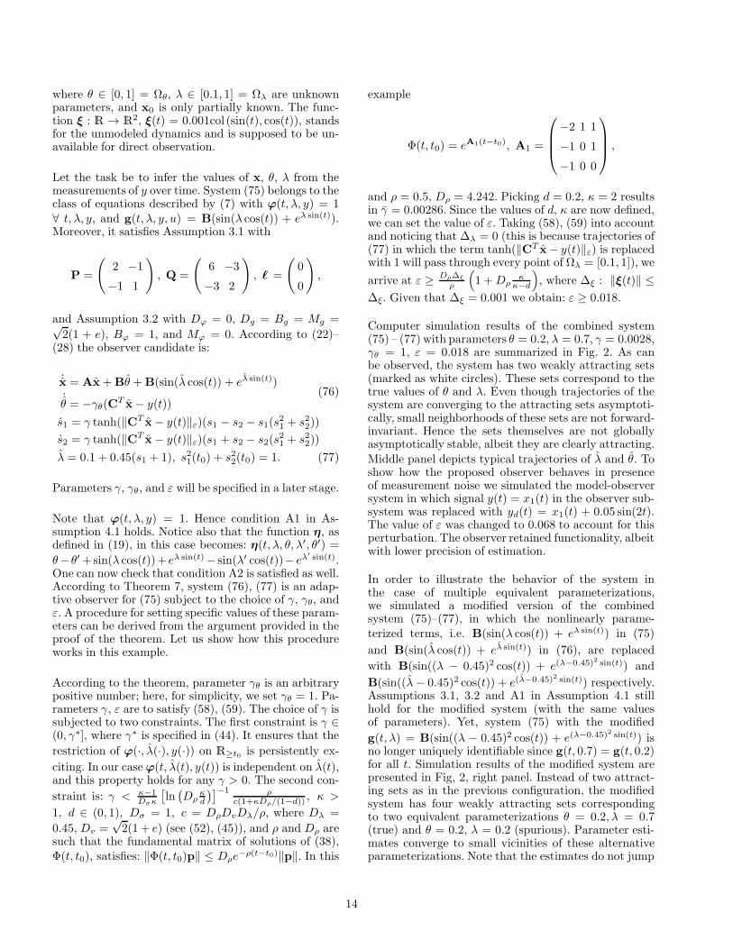
Computer simulation results of the combined system(75) – (77) with parameters θ = 0.2, λ = 0.7, γ = 0.0028,γθ = 1, ε = 0.018 are summarized in Fig. 2. As canbe observed, the system has two weakly attracting sets(marked as white circles). These sets correspond to thetrue values of θ and λ. Even though trajectories of thesystem are converging to the attracting sets asymptoti-cally, small neighborhoods of these sets are not forward-invariant. Hence the sets themselves are not globallyasymptotically stable, albeit they are clearly attracting.

Middle panel depicts typical trajectories of λ and θ. Toshow how the proposed observer behaves in presenceof measurement noise we simulated the model-observersystem in which signal y(t) = x1(t) in the observer sub-system was replaced with yd(t) = x1(t) + 0.05 sin(2t).The value of ε was changed to 0.068 to account for thisperturbation. The observer retained functionality, albeitwith lower precision of estimation.

In order to illustrate the behavior of the system inthe case of multiple equivalent parameterizations,we simulated a modified version of the combinedsystem (75)–(77), in which the nonlinearly parame-terized terms, i.e. B(sin(λ cos(t)) + eλ sin(t)) in (75)

and B(sin(λ cos(t)) + eλ sin(t)) in (76), are replaced

with B(sin((λ − 0.45)2 cos(t)) + e(λ−0.45)2 sin(t)) and

B(sin((λ− 0.45)2 cos(t)) + e(λ−0.45)2 sin(t)) respectively.Assumptions 3.1, 3.2 and A1 in Assumption 4.1 stillhold for the modified system (with the same valuesof parameters). Yet, system (75) with the modified

g(t, λ) = B(sin((λ − 0.45)2 cos(t)) + e(λ−0.45)2 sin(t)) isno longer uniquely identifiable since g(t, 0.7) = g(t, 0.2)for all t. Simulation results of the modified system arepresented in Fig, 2, right panel. Instead of two attract-ing sets as in the previous configuration, the modifiedsystem has four weakly attracting sets correspondingto two equivalent parameterizations θ = 0.2, λ = 0.7(true) and θ = 0.2, λ = 0.2 (spurious). Parameter esti-mates converge to small vicinities of these alternativeparameterizations. Note that the estimates do not jump

14

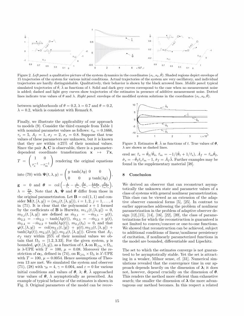
Figure 2. Left panel: a qualitative picture of the system dynamics in the coordinates (s1, s2, θ). Shaded regions depict envelops of15 trajectories of the system for various initial conditions. Actual trajectories of the system are very oscillatory, and individualtrajectories are hardly distinguishable. Qualitatively, their behavior is shown by the black arrowed lines. Middle panel: typical

simulated trajectories of θ, λ as functions of t. Solid and dark grey curves correspond to the case when no measurement noiseis added; dashed and light grey curves show trajectories of the estimates in presence of additive measurement noise. Dotted

lines indicate true values of θ and λ. Right panel: envelops of the modified system solutions in the coordinates (s1, s2, θ).

between neighborhoods of θ = 0.2, λ = 0.7 and θ = 0.2,λ = 0.2, which is consistent with Remark 8.

Finally, we illustrate the applicability of our approachto models (9). Consider the third example from Table 1with nominal parameter values as follows: τm = 0.1666,τs = 5, Af = 1, σf = 2, σs = 0.8. Suppose that truevalues of these parameters are unknown, but it is knownthat they are within ±25% of their nominal values.Since the pair A,C is observable, there is a parameter-dependent coordinate transformation x 7→ Tx,

T =

(

1 0

τ−1s −τ−1

m

)

rendering the original equations

into (70) with Ψ(t, λ, y) =

(

y tanh(λy) 0 0

0 0 y tanh(λy)

)

,

g = 0 and θ = col(

− 1τs

− 1τm

,Af

τm,− 1+σs

τmτs,

Af

τmτs

)

,

λ =σf

Af. Note that A, Ψ and θ differ from those in

the original parametrizaton. Let B = col (1, 1) and con-sider M(t, [λ, y]) = (mij(t, [λ, y])), i = 1, 2, j = 1, . . . , 4in (71). It is clear that the polynomial s + 1 formedby the coefficients of B is Hurwitz, m1,j(t, [λ, y]) = 0,m2,j(t, [λ, y]) are defined as m2,1 = −m2,1 − y(t),m2,2 = −m2,2 − tanh(λy(t)), m2,3 = −m2,3 + y(t),m2,4 = −m2,2 + tanh(λy(t)), m2,j(t0) = 0, and thatϕ(t, [λ, y]) = col(m2,1(t, [y]) + y(t),m2,2(t, [λ, y]) +tanh(λy(t)),m2,3(t, [y]),m2,4(t, [λ, y])). Given that Af ,σf vary within 25% of their nominal values we ob-tain that Ωλ = [1.2, 3.33]. For the given system, y isbounded, ϕ(t, [λ, y]), as a function of t,λ on R≥t0 ×Ωλ,is λ-UPE with T = 100, µ = 0.08. Moreover the re-striction of α5, defined in (74), on R≥t0 ×Ωλ is λ′-UPEwith T = 100, µ = 0.0054. Hence assumptions of Theo-rem 13 are met. We simulated the system and observer(71), (28) with γθ = 4, γ = 0.004, and ε = 0 for various

initial conditions and values of θ, λ; θ, λ approachedtrue values of θ, λ asymptotically as prescribed. Anexample of typical behavior of the estimates is shown inFig. 3. Original parameters of the model can be recov-

Figure 3. Estimates θ, λ as functions of t. True values of θ,λ are shown as dashed lines.

ered as: τs = θ2/θ4, τm = −1/(θ1 + 1/τs), Af = τmθ2,

σs = −θ3τsτm − 1, σf = Af λ. Further examples may befound in the supplementary material [38].

8 Conclusion

We derived an observer that can reconstruct asymp-totically the unknown state and parameter values of aclass of systems with general nonlinear parametrization.This class can be viewed as an extension of the adap-tive observer canonical forms [5], [25]. In contrast toearlier approaches addressing the problem of nonlinearparametrization in the problem of adaptive observer de-sign [12],[15], [14], [16], [22], [39], the class of parame-terizations for which the reconstruction is guaranteed isnot limited to convex/concave or one-to-one functions.We showed that reconstruction can be achieved, subjectto additional conditions of linear/nonlinear persistencyof excitation, if nonlinearly parameterized functions inthe model are bounded, differentiable and Lipschitz.

The set to which the estimates converge is not guaran-teed to be asymptotically stable. Yet the set is attract-ing in a weaker, Milnor sense, cf. [31]. Numerical sim-ulations revealed that the convergence time in our ap-proach depends heavily on the dimension of λ; it doesnot, however, depend crucially on the dimension of θ.This renders the method more efficient than exhaustivesearch; the smaller the dimension of λ the more advan-tageous our method becomes. In this respect a related

15

question arises: is there a “best” parametrization for agiven physical model in the class of systems (7) or (9)?The answer is likely to require quantitative assessmentof the performance of various observers for all admissibleparametrizations. We do not answer this question here,but hope to be able to address it in future.

References

[1] H.D.I. Abarbanel, D. Creveling, R. Farisian, and M. Kostuk.Dynamical state and parameter estimation. SIAM J. AppliedDynamical Systems, 8(4):1341–1381, 2009.

[2] A. Alessandri, M. Baglietto, and G. Battistelli. Moving-horizon state estimation for nonlinear discrete-timesystems: New stability results and approximation schemes.Automatica, 44:1753–1765, 2008.

[3] V.I. Arnold. Mathematical Methods in Classical Mechanics.Springer-Verlag, 1978.

[4] G. Bastin and D. Dochain. On-line Estimation and AdaptiveControl of Bioreactors. Elsevier, 1990.

[5] G. Bastin and M. Gevers. Stable adaptive observers fornonlinear time-varying systems. IEEE Trans. on AutomaticControl, 33(7):650–658, 1988.

[6] G. Besancon. Remarks on nonlinear adaptive observer design.Systems and Control Letters, 41:271–280, 2000.

[7] J.D. Boskovic. Stable adaptive control of a class of first-ordernonlinearly parameterized plants. IEEE Trans. on AutomaticControl, 40(2):347–350, 1995.

[8] C. Cao, A.M. Annaswamy, and A. Kojic. Parameterconvergence in nonlinearly parametrized systems. IEEETrans. on Automatic Control, 48(3):397–411, 2003.

[9] M. Chapell. Structural identifiability of models characterizingsaturable binding: Comparison of pseudo-steady-state andnon-pseudo-steady state model formulations. MathematicalBiosciences, 133:1–20, 1996.

[10] L. Denis-Vidal and Joly-Blanchard. Equivalence andidentifiability analysis of uncontrolled nonlinear dynamicalsystems. Automatica, 40:287–292, 2004.

[11] J. Distefano and C. Cobelli. On parameter and structuralidentifiabiliy: Nonunique observability/reconstructibility foridentifiable systems, other ambiguities, and new definitions.IEEE Trans. on Automatic Control, AC-25(4):830–833, 1980.

[12] M. Farza, M. M’Saad, T. Maatoung, and M. Kamoun.Adaptive observers for nonlinearly parameterized class ofnonlinear systems. Automatica, 45:2292–2299, 2009.

[13] A. Gorban and I. Karlin. Invariant Manifolds for Physicaland Chemical Kinetics. Lecture Notes in Physics, Springer,2005.

[14] H. Grip. State and parameter estimation for linear systemswith nonlinearly parameterized perturbations. In Proceedingsof the 48-th IEEE Conference on Decision and Control, pages8218–8225, 2009.

[15] H.F. Grip, T.A. Johansen, L. Imsland, and G.O. Kaasa.Parameter estimation and compensation in systems withnonlinearly parameterized perturbations. Automatica,46(1):19–28, 2010.

[16] H.F. Grip, A. Saberi, and T.A. Johansen. Estimation ofstates and parameters for linear systems with nonlinearlyparameterized perturbations. Systems and Control Letters,60(9):771–777, 2011.

[17] A. Ilchmann. Universal adaptive stabilization of nonlinearsystems. Dynamics and Control, (7):199–213, 1997.

[18] E. Izhikevich. Dynamical Systems in Neuroscience: TheGeometry of Excitability and Bursting. MIT Press, 2007.

[19] T. Johnson and W. Tucker. Rigorous parameterreconstruction for differential equations with noisy data.Automatica, 44:2422–2426, 2008.

[20] A. Katok and B. Hasselblatt. Introduction to the moderntheory of dynamical systems. Cambridge Univ. Press, 1999.

[21] Z. Lin and C. Knospe. A saturated high-gain contol fora benchmark experiment. In Proceedings of the AmericanControl Conference, pages 2644–2648, 2000.

[22] X. Liu, R. Ortega, H. Su, and J. Chu. On adaptive controlof nonlinearly parameterized nonlinear systems: Towards aconstructive procedure. Systems Control Letters, 60:36–43,2011.

[23] A. Loria. Explicit convergence rates for MRAC-type systems.Automatica, 40(8):1465–1468, 2004.

[24] A. Loria and E. Panteley. Uniform exponential stability oflinear time-varying systems: revisited. Systems and ControlLetters, 47(1):13–24, 2003.

[25] R. Marino. Adaptive observers for single output nonlinearsystems. IEEE Trans. on Automatic Control, 35(9):1054–1058, 1990.

[26] R. Marino and P. Tomei. Global adaptive observers fornonlinear systems via filtered transformations. IEEE Trans.on Automatic Control, 37(8):1239–1245, 1992.

[27] R. Marino and P. Tomei. Global adaptive output-feedbackcontrol of nonlinear systems, part I: Linear parameterization.IEEE Trans. on Automatic Control, 38(1):17–32, 1993.

[28] R. Marino and P. Tomei. Global adaptive output-feedback control of nonlinear systems, part II: Nonlinearparameterization. IEEE Trans. on Automatic Control,38(1):33–48, 1993.

[29] B. Martensson. The order of any stabilizing regulator issufficient a priori information for adaptive stabilization.Systems and Control Letters, 6(2):87–91, 1985.

[30] B. Martensson and J.W. Polderman. Correction andsimplification to “the order of any stabilizing regulator issufficient a priori information for adaptive stabilization”.Systems and Control Letters, 20(6):465–470, 1993.

[31] J. Milnor. On the concept of attractor. Commun. Math.Phys., 99:177–195, 1985.

[32] S. Moreau and J.-C. Trigeassou. Modelling and identificationof a non-linear saturated magnetic circuit: Theoretical studyand experimental results. Mathematics and Computers inSimulation, 71:446–459, 2006.

[33] V.V. Nemytskii and V.V. Stepanov. Qualitative theory ofdifferential equations. Princeton Univ. Press, 1960.

[34] Jean-Baptiste Pomet. Remarks on sufficient information foradaptive nonlinear regulation. In Proceedings of the 31-stIEEE Conference on Decision and Control, pages 1737–1739,1992.

[35] A. Poyton, M. Varziri, K. McAuley, P. McLellan, andJ. Ramsey. Parameter estimation in continuous-time dynamicmodels using principal differential analysis. Computers andChemical Engineering, 30:698–708, 2006.

[36] C.V. Rao, J.B. Rawlings, and D.Q. Mayne. Constrained stateestimation for nonlinear discrete-time systems: Stability andmoving horizon approximation. IEEE Trans. on AutomaticControl, 48:246–258, 2003.

16

[37] P. Rowat and A. Selverston. Modeling the gastric mill centralpattern generator with a relaxation-oscillator network.Journal of Neurophysiology, 70(3):1030–1053, 1993.

[38] I. Tyukin, E. Steur, H. Nijmeijer, and C. van Leeuwen.Supplementary material for: Adaptive observers andparameter estimation for a class of systems nonlinear in theparameters. http://arxiv.org/abs/1304.4020, 2013.

[39] I.Yu. Tyukin, D. V. Prokhorov, and C. van Leeuwen.Adaptation and parameter estimation in systems withunstable target dynamics and nonlinear parametrization.IEEE Trans. on Automatic Control, 52(9):1543–1559, 2007.

[40] I.Yu. Tyukin, E. Steur, H. Nijmeijer, and C. van Leeuwen.Non-uniform small-gain theorems for systems with unstableinvariant sets. SIAM Journal on Control and Optimization,47(2):849–882, 2008.

A Appendix

Lemma 14 Consider y = ky+u(t)+d(t), k ∈ R, u, d :R≥t0 → R, u ∈ C1, d ∈ C0, and let max|u(t)|, |u(t)| ≤B, |d(t)| ≤ ∆ξ. Then ‖y‖∞,[t0,∞) ≤ ε ⇒ ∃ t1(ε) ≥ t0 :

‖u‖∞,[t1(ε),∞) ≤√ε(1 + e|k|

√ε +B) + ∆ξ.

Proof of Lemma 14. Noticing that y(t) for t ≥ t0+T ,T > 0, can be expressed as: y(t) = y(t − T )ekT +∫ t

t−Tek(t−τ)(u(τ) + d(τ))dτ and using the Mean-

value theorem we obtain: y(t) − y(t − T )ekT =

Tek(t−τ ′)(u(τ ′) + d(τ ′)), τ ′ ∈ [t − T, t]. Hence

ε(1+ekT ) ≥ Tek(t−τ ′)(|u(t)|−TB−∆ξ), and ∆ξ+TB+ε(1+ekT )

T min1,ekT ≥ ∆ξ+TB+ ε(1+ekT )

T min1,ek(t−τ′) ≥ |u(t)| for allt ≥ t0+T . Given that T can be chosen arbitrarily we letT =

√ε, and thus |u(t)| ≤ √

ε(1+ek√ε)max1, e−k

√ε+

B√ε+∆ξ ≤

√ε(1 + e|k|

√ε +B) +∆ξ ∀ t ≥ t0 +

√ε.

Proof of Lemma 12. Let us rewrite (64) as

y = a1y + Cx+ u1(t) + d1(t)

˙x = Ax+ ay + bu1(t) +Gu(t) + d(t),

where a = col(a2, . . . , an), C = col(1, 0, . . . , 0),

d(t) = col(d2(t), . . . , dn(t)), and G =(

−b In−1

)

,

A =

(

0 In−2

0 0

)

. Let ‖y(t)‖∞,[t0,∞) ≤ ε and de-

note e(t) = CT x(t) + u1(t). According to Lemma14, there is a t1(ε) > t0 and υ1, υ2 ∈ K such that

‖e(t)‖ = ‖CT x(t)+u1(t)‖ ≤ υ1(ε)+υ2(∆ξ) ∀ t ≥ t1(ε).

Using the notation above we obtain: ˙x = (A −bCT )x + ay(t) + Gu(t) + be(t) + d(t). Matrix

A − bCT = Λ is Hurwitz, and hence there areD, k ∈ R>0 such that ‖eΛ(t−t0)‖ ≤ De−k(t−t0).

Therefore ‖CT x(t) − CT∫ t

t0eΛ(t−τ)Gu(τ)dτ‖ ≤

De−k(t−t0)‖x(t0)‖+Dk (‖a‖ε+‖b‖(υ1(ε)+υ2(∆ξ))+∆ξ).

Noticing that z1 = CT∫ t

t0eΛ(t−τ)Gu(τ)dτ and denot-

ing κ1(ε) = 2Dk (‖a‖ε + ‖b‖υ1(ε)) + υ1(ε), κ2(∆ξ) =

2Dk (∆ξ + ‖b‖υ2(∆ξ)) + υ2(∆ξ) we can conclude that

there is a t′(ε,x0) ≥ t1(ε) such that

‖z1(τ) + u1(τ)‖∞,[t,∞) ≤ κ1(ε) + κ2(∆ξ) ∀ t ≥ t′(ε).

Noticing that y(t),d(t) ≡ 0 ⇒ e(t) ≡ 0 ensures that(66) holds too.

Proof of Lemma 10. Consider J(λ, t) = zT( ∫ t+T

t

α(τ,λ)αT (τ,λ)dτ)

z =∫ t+T

t ‖zTα(τ,λ)‖2, where

z ∈ Rn+m, z 6= 0, for t ∈ R≥t0 . According to C2 we

have: J(λ, t) ≥ µ‖z‖2 ∀ λ ∈ Ωλ. Let λ : R≥t0 → Ωλ

be a differentiable function, and consider J(λ(t), t) −∫ t+T

t‖zTα(τ, λ(τ))‖2dτ =

∫ t+T

t‖zTα(τ, λ(t))‖2

− ‖zTα(τ, λ(τ))‖2dτ =∫ t+T

t ‖zTα(τ, λ(t))‖2 −zTα(τ, λ(t))αT (τ, λ(τ))z+ zTα(τ, λ(t))αT (τ, λ(τ))z−‖zTα(τ, λ(τ))‖2dτ =

∫ t+T

tzTα(τ, λ(t))[αT (τ, λ(t)) −

αT (τ, λ(τ))]z +∫ t+T

tzT [α(τ, λ(t)) − α(τ, λ(τ))]

αT (τ, λ(τ))zdτ . Applying the Cauchy-Schwarz in-equality to the last equality, and invoking C4 and

C3 we obtain: J(λ(t), t) −∫ t+T

t ‖zTα(τ, λ(τ))‖2dτ ≤( ∫ t+T

t‖zT [α(τ, λ(t)) − α(τ, λ(τ))]‖2dτ

)12 2MT ‖z‖ ≤

2DMT 2 ‖z‖2 maxτ∈[t,t+T ] ‖ ˙λ(τ)‖. Thus (39), (40)ensure that

∫ t+T

t‖zTα(τ, λ(τ))‖2dτ ≥ J(λ(t), t) −

rµ‖z‖2. This, in accordance with C2, guarantees

that∫ t+T

t ‖zTα(τ, λ(τ))‖2dτ ≥ (1 − r)µ‖z‖2. Hence

α(t, λ(t)) is persistently exciting in the sense of Defi-nition 2. The value of (1 − r)µ does not depend on the

choice of λ as long as (40), (39) hold. Finally, notice

that C4 and (39) guarantee boundedness of α(·, λ(·))and its derivative: max‖α(t, λ(t))‖, ‖α(t, λ(t))‖ ≤M + MMλ = M + µr

2DT 2 . Taking C1 and Theorem 3into account we conclude that the lemma follows.

Proof of Lemma 11. According to conditions of thelemma, (57), we conclude that h(t0) ≥ 0. Introduce astrictly decreasing sequence: σi, i = 0, 1, . . . , σi =(1/κ)i, κ ∈ (1,∞). Further, let ti, i = 1, . . . , t1 <t2 < · · · < tn < · · · be an ordered infinite sequence:

h(ti) = σih(t0). (A.1)

If ti satisfying (A.1) does not exist then it is clear thath(t0) ≥ h(t) ≥ 0 for all t ≥ t0. Hence, in accordancewith (29), x(·) is bounded for all t ≥ t0, and nothingremains to be proven. Let us now show that if (56), (57),and (A.1) hold then

h(t) → 0 ⇒ t → ∞. (A.2)

17

Consider Ti = ti − ti−1. It is clear from (55) that

TiDγ maxτ∈[ti−1,ti]

‖x(τ)+d(τ)‖ε ≥ h(t0)(σi−1−σi). (A.3)

In addition, maxτ∈[ti−1,ti] ‖x(τ)+ d(τ)‖ε = ‖x(τ) +d(τ)‖∞,[ti−1,ti] −ε if ‖x(τ) + d(τ)‖∞,[ti−1,ti] > ε, andmaxτ∈[ti−1,ti] ‖x(τ) + d(τ)‖ε = 0 overwise, we can seefrom (A.3) that

Ti ≥

h(t0)(σi−1−σi)Dγ

1‖x(τ)+d(τ)‖∞,[ti−1,ti]

−ε ,

‖x(τ) + d(τ)‖∞,[ti−1,ti] > ε;

∞, ‖x(τ) + d(τ)‖∞,[ti−1,ti] ≤ ε.

(A.4)

Consider the case when ‖x(τ) + d(τ)‖∞,[ti−1,ti] − ε > 0for all i = 1, 2, . . . . Let us pick

τ∗ = −1 (d/κ) , d ∈ (0, 1), (A.5)

and select the value of Dγ such that (57) holds. Giventhat ‖x(τ) + d(τ)‖∞,[t0,t1] − ε ≤ (0)‖x(t0)‖+ ch(t0) +∆+∆d−ε, conditions (57), (56), and (A.5) implyDγ ≤κ−1κ

h(t0)(0)‖x(t0)‖+c|h(t0)|

1τ∗

≤ h(t0)(σ0−σ1)(‖x(τ)+d(τ)‖∞,[t0,t1]−ε)

1τ∗.

This, as follows from (A.4), guarantees that T1 ≥ τ∗.

Without loss of generality suppose that there is an i ≥ 2:Tj ≥ τ∗ for all 1 ≤ j ≤ i − 1. Let us show that Ti−1 ≥τ∗ ⇒ Ti ≥ τ∗. This will ensure that (A.2) is satisfied andthat the lemma hold. Consider ‖x(τ)‖∞,[ti−1,ti]; (54) and(A.1) imply that: ‖x(τ)‖∞,[ti−1,ti] ≤ (0)‖x(ti−1)‖ +cσi−1h(t0) + ∆. Hence

‖x(τ)‖∞,[ti−1,ti] ≤ (0)[(Ti−1)‖x(ti−2)‖+ cσi−2h(t0)]

+ (0)∆ + ch(t0)σi−1 +∆ ≤ (0)(τ∗)‖x(ti−2)‖+ P1,

where P1 = (0)cσi−2h(t0) + cσi−1h(t0) + (0)∆ + ∆.Invoking (54) again results in

‖x(τ)‖∞,[ti−1,ti] ≤ (0)2(τ∗)‖x(ti−3)‖+ P2,

where P2 = ch(t0)(0)[(τ∗)σi−3 +σi−2]+ cσi−1h(t0)+

(0)[(τ∗)∆ +∆] + ∆, and

‖x(τ)‖∞,[ti−1,ti] ≤ (0)3(τ∗)‖x(ti−4)‖+ P3,

where P3 = ch(t0)(0)[2(τ∗)σi−4 + (τ∗)σi−3 +

σi−2] + cσi−1h(t0) + ∆(0)[(τ∗)2 + (τ∗) + 1] +

∆ = ch(t0)(0)[∑2

j=0 j(τ∗)σi−j−2] + ch(t0)σi−1 +

∆(0)[∑2

j=0 j(τ∗)] + ∆. After i− 1 steps we obtain

‖x(τ)‖∞,[ti−1,ti] ≤ (0)i−1(τ∗)‖x(t0)‖ + Pi−1, (A.6)

withPi−1 = ch(t0)(0)[∑i−2

j=0 j(τ∗)σi−j−2]+ch(t0)σi−1

+ ∆(0)[∑i−2

j=0 j(τ∗)] + ∆. The values of Ti, as follows

from (A.4), are bounded from below by:

Ti ≥ σi−1−σi

σi−1Dγσ−1i−1

h(t0)

(‖x(τ)+d(τ)‖∞,[ti−1,ti]−ε)

. (A.7)

Consider σ−1i−1(‖x(τ)+d(τ)‖∞,[ti−1,ti]−ε). Taking (A.6)

into account we derive that:

σ−1i−1(‖x(τ) + d(τ)‖∞,[ti−1,ti] − ε) ≤ (0)i−1(τ∗)×

κi−1‖x(t0)‖+ ki−1Pi−1 + ki−1∆d − ki−1ε =

(0)i−1(τ∗)κi−1‖x(t0)‖+ ch(t0)(0)κ[∑i−2

j=0 j(τ∗)κj ]

+ch(t0) + κi−1[∆((0)∑i−2

j=0 j(τ∗) + 1) + ∆d − ε].

Noticing that τ∗ is chosen in accordance with (A.5) onecan therefore obtain:

σ−1i−1(‖x(τ) + d(τ)‖∞,[ti−1,ti] − ε) ≤ (0)‖x(t0)‖+

ch(t0) + ch(t0)(0)κ∑i−2

j=0 dj+

κi−1[∆((0)∑i−2

j=0dκ

j+ 1) + ∆d − ε]

≤ (0)‖x(t0)‖+ ch(t0)(1 +(0)κ1−d )+

ki−1[∆( (0)1−d/k + 1) + ∆d − ε].

Condition (56) implies that ∆( (0)1−d/k +1)+∆d − ε ≤ 0.

Hence σ−1i−1(‖x(τ)+d(τ)‖∞,[ti−1 ,ti]−ε) ≤ (0)‖x(t0)‖+

ch(t0)(1 + (0)κ1−d ). Substituting the latter estimate into

(A.7) and using (57) yields Ti ≥ τ∗. Thus h(·) is boundedfor t ≥ t0, and hence so is x(·).

Proof of Theorem 13. Let Λ0 = A − BCTA,

G0 = In − BCT . Consider ϕ(t, λ(t), T1) = CTA∫ t

t−T1

eΛ0(t−τ)G0 Ψ(τ, λ(t), y(τ))dτ + CTΨ(t, λ(t), y(t)). Itis clear that for any ε1 > 0 there are T1, t1 sufficientlylarge and γ1 sufficiently small:

‖ϕ(t, λ(t), T1)−ϕ(t, λ(t), y(t), [λ, y])‖ < ε1 (A.8)

for all γ ∈ (0, γ1) and t ≥ t1 ≥ t0. Indeed, con-

sider δ1(T1, t) = CTAeΛ0T1∫ t−T1

t0eΛ0(t−T1−τ)G0

Ψ(τ, λ(τ), y(τ))dτ , δ2(T1, t) = CTA∫ t

t−T1eΛ0(t−τ)

G0(Ψ(τ, λ(τ), y(τ)) − Ψ(τ, λ(t), y(τ)))dτ , pick ε1 >0, and let T1 be so large that |δ1(T1, t)| < ε1/2for t ≥ t0 + T1. Let γ1 ∈ R>0 be so small that|δ2(T1, t)| < ε1/2 for all t ≥ t0 + T1 (such a choice is

always possible due to that Ψ is Lipschitz in λ). Notic-

ing that ϕ(t, λ(t), y(t), [λ, y]) = δ1(T1, t) + δ2(T1, t) +

ϕ(t, λ(t), T1) we can conclude that (A.8) holds.

Given that the restriction of ϕ(t,λ, y(t), [λ, y]) (as afunction of t, λ) on R≥t0 ×Ωλ is λ-UPE with T, µ, thereis a ε1 in (A.8) such that ϕ(t,λ, T1) ∈ λUPE(T, µ− ǫ),

18

ǫ ∈ (0, µ/3). On the other hand (see the first part of the

proof of Lemma 10), there is a γ2 such that ϕ(t, λ(t), T1)is persistently exciting with parameters T, µ − 2ǫ forall γ ∈ (0, γ2). Choosing γ ∈ (0,minγ1, γ2) and tak-ing (A.8) into account we conclude that the restriction

of ϕ(·, λ(·), y(·), [λ, y]) on R≥t2 is persistently exciting(t2 > t1 > t0) provided that ε1 is small enough and t2is sufficiently large. Thus, invoking the argument pre-sented in Part 2 of the proof of Theorem 7 we can con-clude that (61) and (60) hold for the combined system.Convergence of state and parameter estimates can nowbe shown similarly to the 3d part of the proof of Theo-rem 7.

19