Embed Size (px)
Citation preview

PDAF Tutorial
Implementation of the analysis step
in online mode with a parallel model
http://pdaf.awi.de
V1.6 – 2019-12-12

PDAF tutorial – Analysis step in online mode with a parallel model
We demonstrate the implementation
of an online analysis step with PDAF
with a model that is parallelized
using the template routines provided by PDAF
The example code is part of the PDAF source code package downloadable at http://pdaf.awi.de
Implementation Tutorial for PDAF online and parallel model

PDAF tutorial – Analysis step in online mode with a parallel model
Implementation Tutorial for PDAF online / parallel model
This is just an example!
For the complete documentation of PDAF’s interface
see the documentation
at http://pdaf.awi.de
PDAF tutorial – Analysis step in online mode with a parallel model
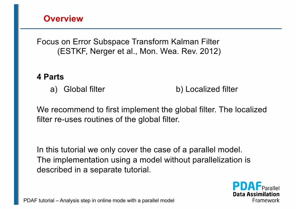
Overview
Focus on Error Subspace Transform Kalman Filter (ESTKF, Nerger et al., Mon. Wea. Rev. 2012)
4 Partsa) Global filter b) Localized filter
We recommend to first implement the global filter. The localized filter re-uses routines of the global filter.
In this tutorial we only cover the case of a parallel model. The implementation using a model without parallelization is described in a separate tutorial.

PDAF tutorial – Analysis step in online mode with a parallel model
0a) Files for the Tutorial
PDAF tutorial – Analysis step in online mode with a parallel model
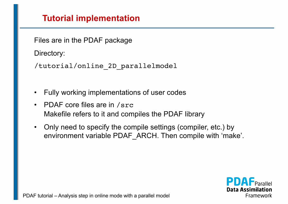
Tutorial implementation
Files are in the PDAF package
Directory:
/tutorial/online_2D_parallelmodel
• Fully working implementations of user codes
• PDAF core files are in /srcMakefile refers to it and compiles the PDAF library
• Only need to specify the compile settings (compiler, etc.) by environment variable PDAF_ARCH. Then compile with ‘make’.
PDAF tutorial – Analysis step in online mode with a parallel model
Template files for online mode
Directory: /templates/online
• Contains all required files
• Contains also command line parser(convenient but not required)
To generate your own implementation:1. Copy content of directory
e.g. into sub-directory of model source code2. Add calls to interface routines to model code3. Complete user-routines for your model4. Adapt compilation (e.g. Makefile) and compile5. Run with assimilation options
PDAF tutorial – Analysis step in online mode with a parallel model
PDAF library
PDAF tutorial – Analysis step in offline mode
Directory: /src
• The PDAF library is not part of the template• PDAF is compiled separately as a library
and linked when the assimilation program is compiled• Makefile includes a compile step for the PDAF library• One can also cd to /src and run ‘make’ there
(requires setting of PDAF_ARCH)
$PDAF_ARCH
• Environment variable to specify the compile specifications• Definition files in /make.arch• Define by, e.g.
setenv PDAF_ARCH linux_gfortran (tcsh/csh)export PDAF_ARCH=linux_gfortran (bash)

PDAF tutorial – Analysis step in online mode with a parallel model
0b) The parallelized model
PDAF tutorial – Analysis step in online mode with a parallel model
Simple assimilation problem
• 2-dimensional model domain
• One single field (like temperature)
• Direct measurements of the field
• Data gaps (i.e. data at selected grid points)
• Same error estimate for all observations
• Observation errors are not correlated(diagonal observation error covariance matrix)
• Simple time stepping:Shift field in vertical direction one grid point per time step
PDAF tutorial – Analysis step in online mode with a parallel model
2D „Model“
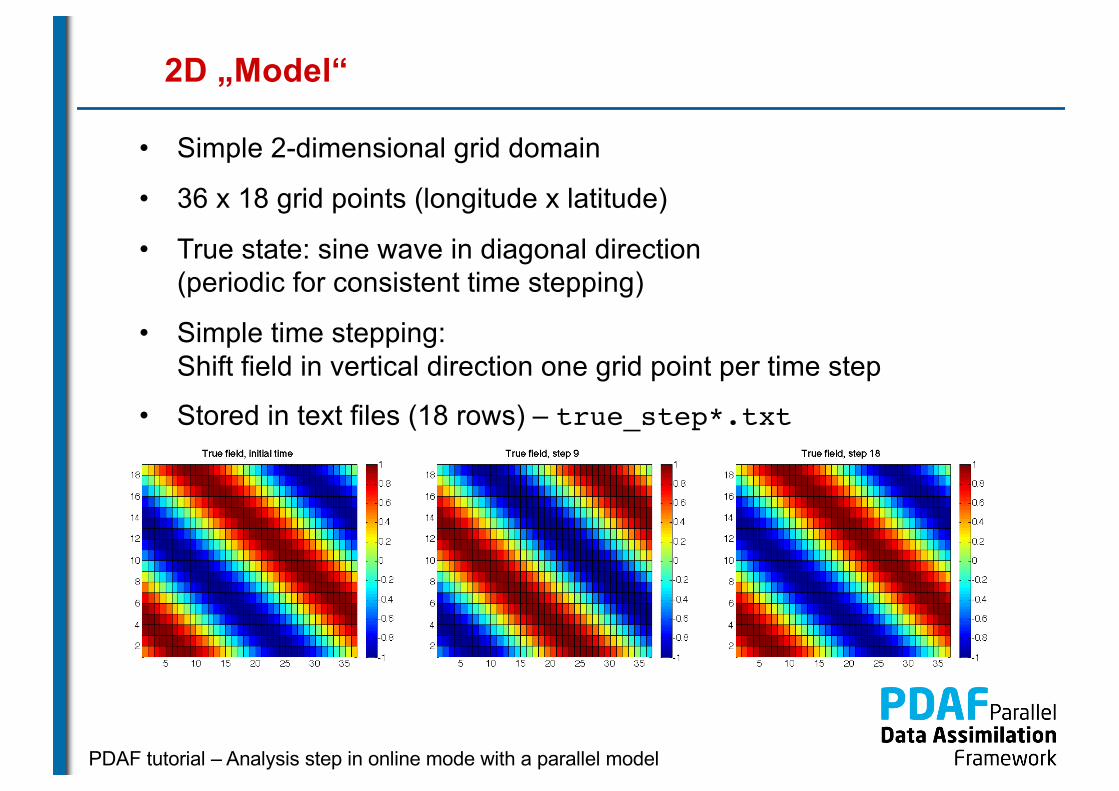
• Simple 2-dimensional grid domain
• 36 x 18 grid points (longitude x latitude)
• True state: sine wave in diagonal direction (periodic for consistent time stepping)
• Simple time stepping:Shift field in vertical direction one grid point per time step
• Stored in text files (18 rows) – true_step*.txt
PDAF tutorial – Analysis step in online mode with a parallel model
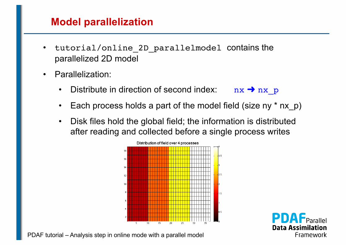
Model parallelization
• tutorial/online_2D_parallelmodel contains the parallelized 2D model
• Parallelization:
• Distribute in direction of second index: nx� nx_p
• Each process holds a part of the model field (size ny * nx_p)
• Disk files hold the global field; the information is distributed after reading and collected before a single process writes
PDAF tutorial – Analysis step in online mode with a parallel model
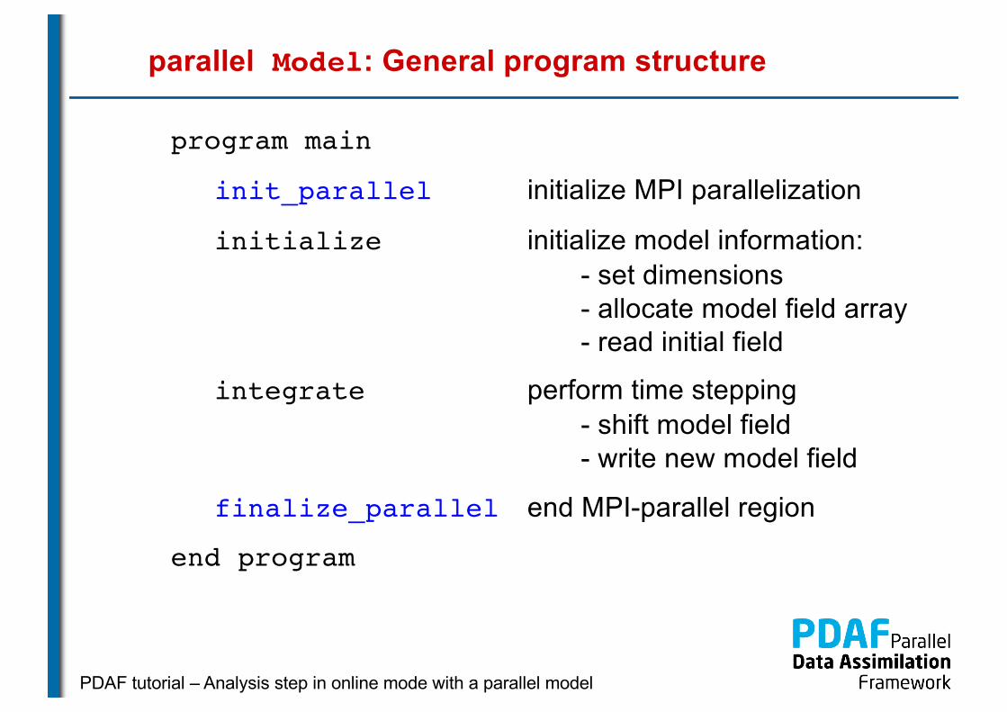
parallel Model: General program structure
program main
init_parallel initialize MPI parallelization
initialize initialize model information:- set dimensions- allocate model field array- read initial field
integrate perform time stepping- shift model field- write new model field
finalize_parallel end MPI-parallel region
end program
PDAF tutorial – Analysis step in online mode with a parallel model
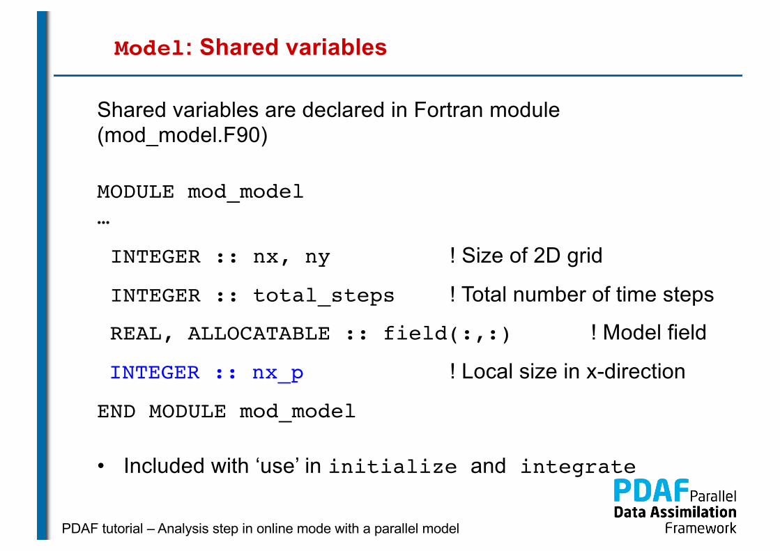
Model: Shared variables
Shared variables are declared in Fortran module(mod_model.F90)
MODULE mod_model…
INTEGER :: nx, ny ! Size of 2D grid
INTEGER :: total_steps ! Total number of time steps
REAL, ALLOCATABLE :: field(:,:) ! Model field
INTEGER :: nx_p ! Local size in x-direction
END MODULE mod_model
• Included with ‘use’ in initialize and integrate
PDAF tutorial – Analysis step in online mode with a parallel model
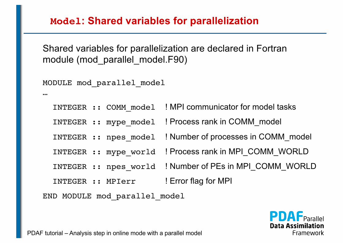
Model: Shared variables for parallelization
Shared variables for parallelization are declared in Fortran module (mod_parallel_model.F90)
MODULE mod_parallel_model…
INTEGER :: COMM_model ! MPI communicator for model tasks
INTEGER :: mype_model ! Process rank in COMM_model
INTEGER :: npes_model ! Number of processes in COMM_model
INTEGER :: mype_world ! Process rank in MPI_COMM_WORLD
INTEGER :: npes_world ! Number of PEs in MPI_COMM_WORLD
INTEGER :: MPIerr ! Error flag for MPI
END MODULE mod_parallel_model
PDAF tutorial – Analysis step in online mode with a parallel model
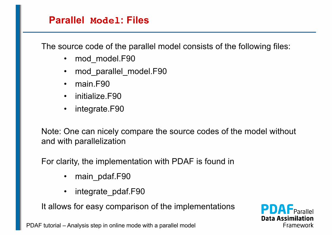
Parallel Model: Files
The source code of the parallel model consists of the following files:• mod_model.F90• mod_parallel_model.F90• main.F90• initialize.F90• integrate.F90
Note: One can nicely compare the source codes of the model without and with parallelization
For clarity, the implementation with PDAF is found in
• main_pdaf.F90
• integrate_pdaf.F90
It allows for easy comparison of the implementations
PDAF tutorial – Analysis step in online mode with a parallel model
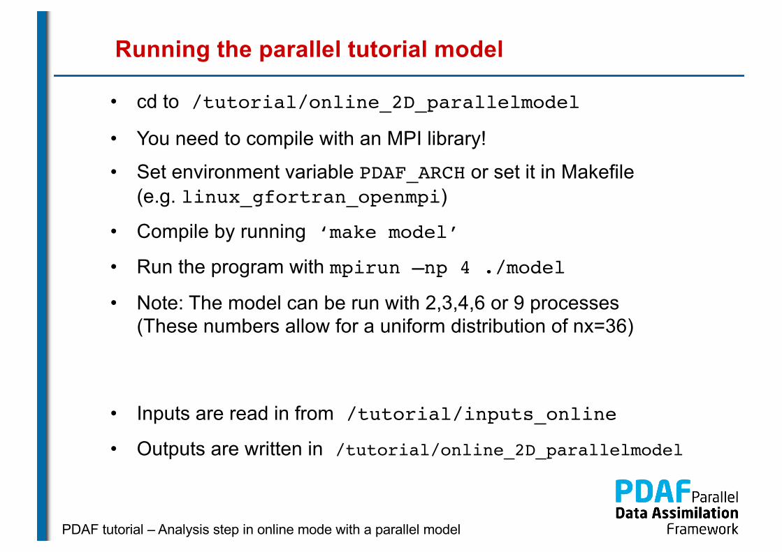
Running the parallel tutorial model
• cd to /tutorial/online_2D_parallelmodel
• You need to compile with an MPI library!
• Set environment variable PDAF_ARCH or set it in Makefile(e.g. linux_gfortran_openmpi)
• Compile by running ‘make model’
• Run the program with mpirun –np 4 ./model
• Note: The model can be run with 2,3,4,6 or 9 processes(These numbers allow for a uniform distribution of nx=36)
• Inputs are read in from /tutorial/inputs_online
• Outputs are written in /tutorial/online_2D_parallelmodel

PDAF tutorial – Analysis step in online mode with a parallel model
Observations
• Add random error to true state (standard deviation 0.5)
• Select a set of observations at 28 grid points
• File storage (in inputs_online):
text file, full 2D field, -999 marks ‘no data’ – obs_step*.txtone file for each time step
PDAF tutorial – Analysis step in online mode with a parallel model
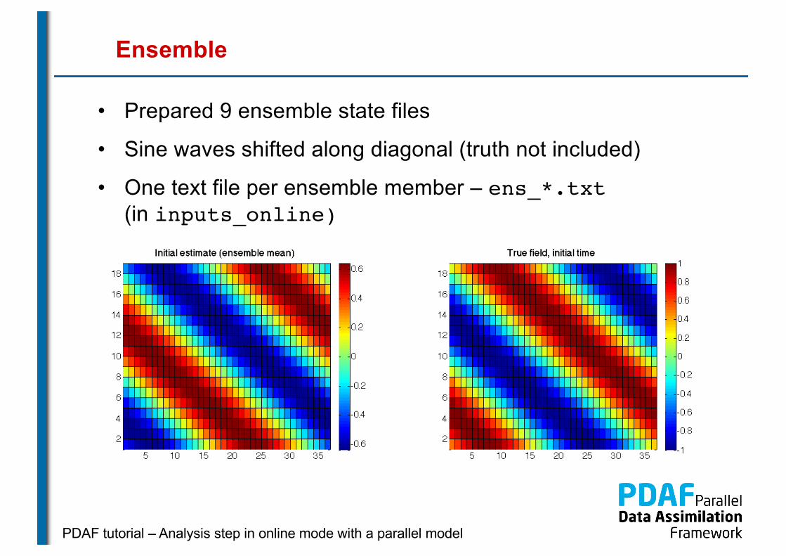
Ensemble
• Prepared 9 ensemble state files
• Sine waves shifted along diagonal (truth not included)
• One text file per ensemble member – ens_*.txt(in inputs_online)
PDAF tutorial – Analysis step in online mode with a parallel modelsdsdsds
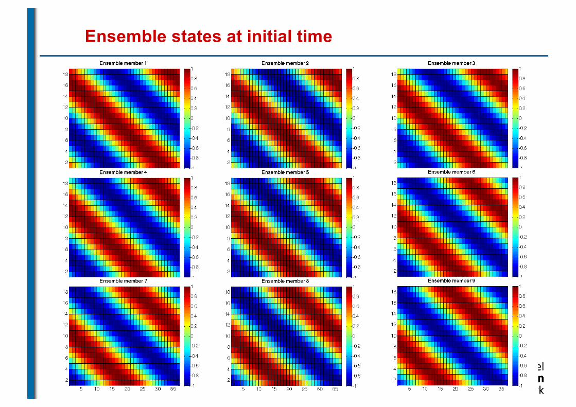
Ensemble states at initial time
PDAF tutorial – Analysis step in online mode with a parallel model
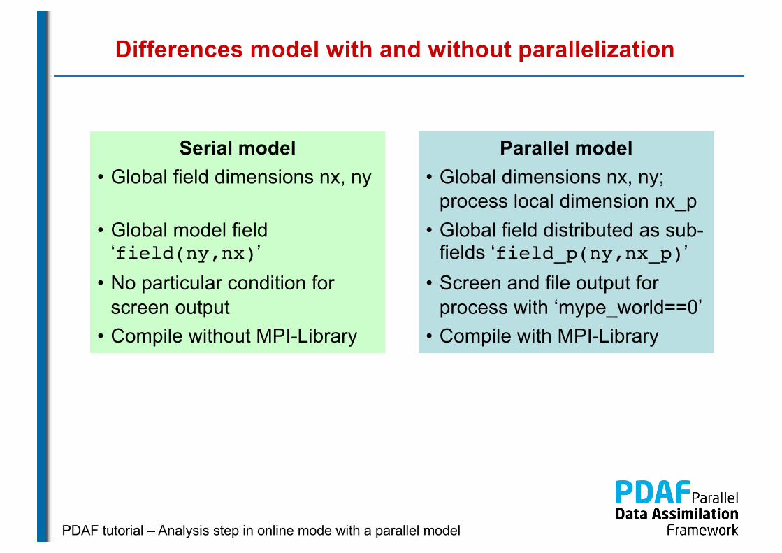
Differences model with and without parallelization
Serial model• Global field dimensions nx, ny
• Global model field ‘field(ny,nx)’
• No particular condition for screen output
• Compile without MPI-Library
Parallel model• Global dimensions nx, ny;
process local dimension nx_p• Global field distributed as sub-
fields ‘field_p(ny,nx_p)’• Screen and file output for
process with ‘mype_world==0’• Compile with MPI-Library

PDAF tutorial – Analysis step in online mode with a serial model
0c) state vector and observation vector
PDAF tutorial – Analysis step in online mode with a parallel model
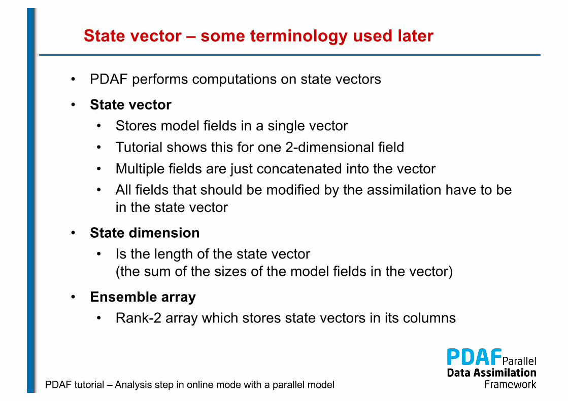
State vector – some terminology used later
• PDAF performs computations on state vectors
• State vector• Stores model fields in a single vector• Tutorial shows this for one 2-dimensional field• Multiple fields are just concatenated into the vector• All fields that should be modified by the assimilation have to be
in the state vector
• State dimension• Is the length of the state vector
(the sum of the sizes of the model fields in the vector)
• Ensemble array• Rank-2 array which stores state vectors in its columns
PDAF tutorial – Analysis step in online mode with a parallel model
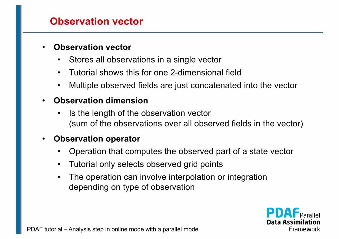
Observation vector
• Observation vector• Stores all observations in a single vector• Tutorial shows this for one 2-dimensional field• Multiple observed fields are just concatenated into the vector
• Observation dimension• Is the length of the observation vector
(sum of the observations over all observed fields in the vector)
• Observation operator• Operation that computes the observed part of a state vector• Tutorial only selects observed grid points• The operation can involve interpolation or integration
depending on type of observation
PDAF tutorial – Analysis step in online mode with a parallel model
0c) PDAF online mode
PDAF tutorial – Analysis step in online mode with a parallel model
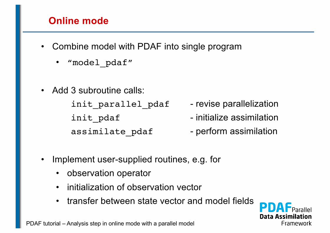
Online mode
• Combine model with PDAF into single program
• “model_pdaf”
• Add 3 subroutine calls:init_parallel_pdaf - revise parallelizationinit_pdaf - initialize assimilationassimilate_pdaf - perform assimilation
• Implement user-supplied routines, e.g. for• observation operator• initialization of observation vector• transfer between state vector and model fields
PDAF tutorial – Analysis step in online mode with a parallel model
Aaaaaaaa
Aaaaaaaa
aaaaaaaaa
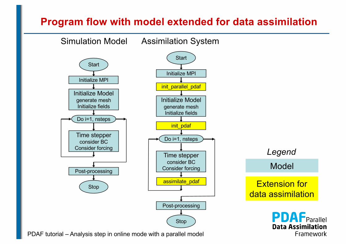
Start
Stop
Do i=1, nsteps
Initialize Modelgenerate meshInitialize fields
Time stepperconsider BC
Consider forcing
Post-processingModel
Extension for data assimilation
Aaaaaaaa
Aaaaaaaa
aaaaaaaaa
Start
Stop
Initialize Modelgenerate meshInitialize fields
Time stepperconsider BC
Consider forcing
Post-processing
init_parallel_pdaf
Do i=1, nsteps
init_pdaf
assimilate_pdaf
Simulation Model Assimilation System
Legend
Initialize MPIInitialize MPI
Program flow with model extended for data assimilation

PDAF tutorial – Analysis step in online mode with a parallel model
Fully parallel configuration
• Tutorial shows implementation for a fully parallel case
➜ Number of processes equals ensemble size times number of processes used for a single model task!
• For a more flexible (and complicated) configuration see PDAF’s online guide
PDAF tutorial – Analysis step in online mode with a parallel model
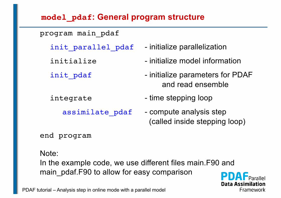
model_pdaf: General program structure
program main_pdaf
init_parallel_pdaf - initialize parallelization
initialize - initialize model information
init_pdaf - initialize parameters for PDAF and read ensemble
integrate - time stepping loop
assimilate_pdaf - compute analysis step(called inside stepping loop)
end program
Note: In the example code, we use different files main.F90 and main_pdaf.F90 to allow for easy comparison

PDAF tutorial – Analysis step in online mode with a parallel model
mod_assimilation.F90
Fortran module
• Declares the parameters used to configure PDAF
• Will be included (with ‘use’) in the user-written routines
• Additions to template necessary for observation handling

PDAF tutorial – Analysis step in online mode with a parallel model
0d) Inserting subroutine calls
PDAF tutorial – Analysis step in online mode with a parallel model
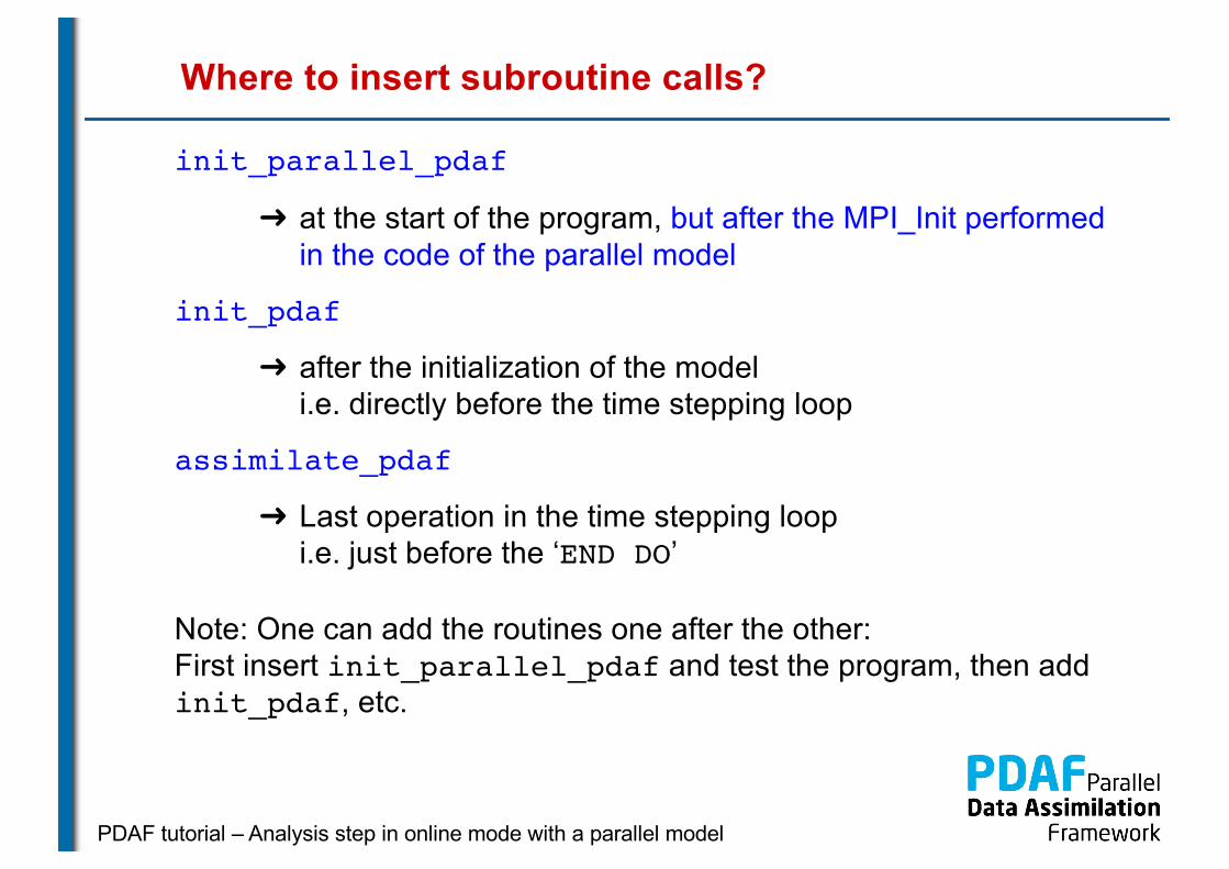
Where to insert subroutine calls?
init_parallel_pdaf
➜ at the start of the program, but after the MPI_Init performed in the code of the parallel model
init_pdaf
➜ after the initialization of the model i.e. directly before the time stepping loop
assimilate_pdaf
➜ Last operation in the time stepping loopi.e. just before the ‘END DO’
Note: One can add the routines one after the other: First insert init_parallel_pdaf and test the program, then add init_pdaf, etc.
PDAF tutorial – Analysis step in online mode with a parallel model
init_parallel_pdaf.F90
• It is fully implemented template usable with small adaptions
• Required adaptions
• Include MPI variables from module of the model:MPI_COMM_WORLD, COMM_model, mype_model, npes_model(the latter three variables might be named differently in a model)
• init_parallel_pdaf defines a model communicatorcomm_model(actually it’s a set for communicators, one for each model task)
• Set communicator of the parallel model to comm_model at the end if init_parallel_pdaf:“my_models_communicator” = comm_model(include my_models_communicator from module of model)
• Set variables for number of processes in model and rank of a process (npes_model, mype_model) at end of routine

PDAF tutorial – Analysis step in online mode with a parallel model
init_parallel_pdaf.F90 (2)
• Parallelization variables for PDAF are declared in Fortran
module
mod_parallel_pdaf
• Important variable:
n_modeltasks
• Defines number of concurrent model integrations.
• Has to be equal to ensemble size
• In the example: Read as ‘dim_ens’ from command line
(using subroutine ‘parse’)
• Important: If the parallel model uses MPI_COMM_WORLD, this
has to be replaced! (MPI_COMM_WORLD denotes always all
processes in the program)
PDAF tutorial – Analysis step in online mode with a parallel model
init_parallel_pdaf.F90 (3) - Example
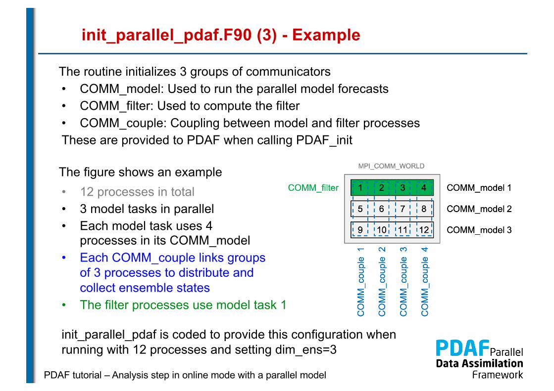
The routine initializes 3 groups of communicators• COMM_model: Used to run the parallel model forecasts• COMM_filter: Used to compute the filter• COMM_couple: Coupling between model and filter processesThese are provided to PDAF when calling PDAF_init
The figure shows an example• 12 processes in total• 3 model tasks in parallel• Each model task uses 4
processes in its COMM_model• Each COMM_couple links groups
of 3 processes to distribute and collect ensemble states
• The filter processes use model task 1
init_parallel_pdaf is coded to provide this configuration when running with 12 processes and setting dim_ens=3

PDAF tutorial – Analysis step in online mode with a parallel model
init_pdaf.F90
Routine sets parameters for PDAF, calls PDAF_initto initialize the data assimilation, and calls PDAF_get_state to prepare the ensemble integrations:
Template contains list of available parameters(declared in and used from mod_assimilation)
Independent of the filter algorithm:• Include information on size of model fields from model• Define dimension of decomposed state vector
dim_state_p = nx_p * ny
In call to PDAF_init, the name of the user-supplied routine for ensemble initialization routine is specified:
init_ens_pdaf
PDAF tutorial – Analysis step in online mode with a parallel model
init_pdaf.F90 (II)
In call to PDAF_get_state, the names of 3 user-supplied routines are specified:
next_observation_pdaf- Set number of time steps in forecast phase
distribute_state_pdaf- Initialize model fields from state
vector
prepoststep_ens_pdaf- poststep routine (compute estimated errors, write state estimate, etc.)
Initially, one can just copy the template routines. One can adapt them later to the particular application.
PDAF tutorial – Analysis step in online mode with a parallel model
assimilate_pdaf.F90
Routine just calls a filter-specific routine like
PDAF_assimilate_estkf
We don’t insert PDAF_assimilate_estkf directly into the model code
➜ because, we need to declare all user-supplied routines as ‘EXTERNAL’. This could clutter the model code.
Filter-specific user routines are described next. Initially, one can just copy the template routines.
Note: Template contains calls for PDAF_assimilate_estkf and PDAF_assimilate_lestkf. Need to adapt for other filters

PDAF tutorial – Analysis step in online mode with a parallel model
Differences online and offline
• If you’ve studied the tutorial for offline mode
Offline• Separate programs for
model and assimilation• Needed to implement
routine intialize
• Grid dimensions declared in mod_assimilation
• Ensemble information read from files
• mod_assimilationcontains all field and assimilation variables
Online• Extend model program for
assimilation• Operations in initialize
given by model; no changes for assimilation!
• Grid dimensions defined in model code (mod_model)
• Ensemble information provided by model fields
• mod_assimilation only contains variables for assimilation
PDAF tutorial – Analysis step in online mode with a parallel model
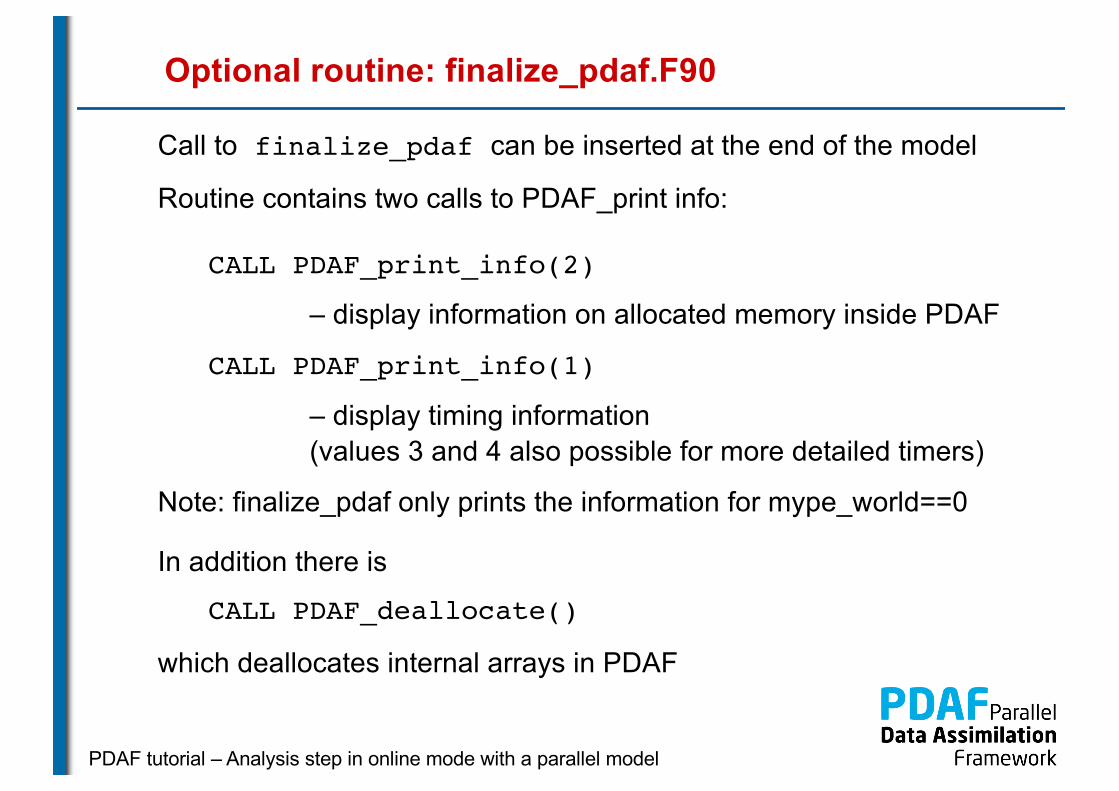
Optional routine: finalize_pdaf.F90
Call to finalize_pdaf can be inserted at the end of the model
Routine contains two calls to PDAF_print info:
CALL PDAF_print_info(2)
– display information on allocated memory inside PDAF
CALL PDAF_print_info(1)
– display timing information(values 3 and 4 also possible for more detailed timers)
Note: finalize_pdaf only prints the information for mype_world==0
In addition there is
CALL PDAF_deallocate()
which deallocates internal arrays in PDAF

PDAF tutorial – Analysis step in online mode with a parallel model
0e) Forecast phase
PDAF tutorial – Analysis step in online mode with a parallel model
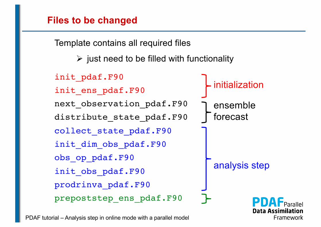
Files to be changed
Template contains all required files
Ø just need to be filled with functionality
init_pdaf.F90init_ens_pdaf.F90next_observation_pdaf.F90distribute_state_pdaf.F90collect_state_pdaf.F90init_dim_obs_pdaf.F90obs_op_pdaf.F90init_obs_pdaf.F90prodrinva_pdaf.F90prepoststep_ens_pdaf.F90
initialization
analysis step
ensemble forecast
PDAF tutorial – Analysis step in online mode with a parallel model
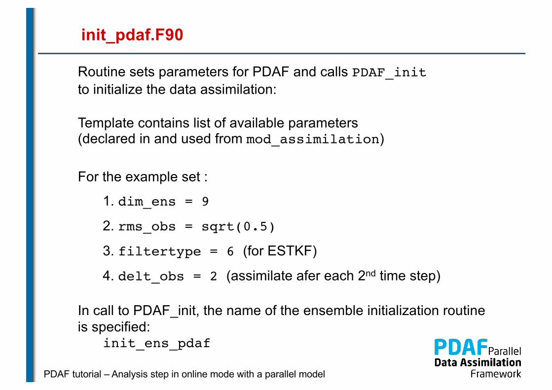
init_pdaf.F90
Routine sets parameters for PDAF and calls PDAF_initto initialize the data assimilation:
Template contains list of available parameters(declared in and used from mod_assimilation)
For the example set :
1. dim_ens = 9
2. rms_obs = sqrt(0.5)
3. filtertype = 6 (for ESTKF)
4. delt_obs = 2 (assimilate afer each 2nd time step)
In call to PDAF_init, the name of the ensemble initialization routine is specified:
init_ens_pdaf
PDAF tutorial – Analysis step in online mode with a parallel model
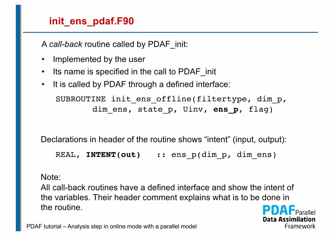
init_ens_pdaf.F90
A call-back routine called by PDAF_init:
• Implemented by the user
• Its name is specified in the call to PDAF_init
• It is called by PDAF through a defined interface:
SUBROUTINE init_ens_offline(filtertype, dim_p, dim_ens, state_p, Uinv, ens_p, flag)
Declarations in header of the routine shows “intent” (input, output):
REAL, INTENT(out) :: ens_p(dim_p, dim_ens)
Note:
All call-back routines have a defined interface and show the intent of
the variables. Their header comment explains what is to be done in
the routine.

PDAF tutorial – Analysis step in online mode with a parallel model
init_ens_pdaf.F90 (2)
Initialize ensemble matrix ens_p for the start time of the assimilation
1. Include nx, ny, nx_p with use mod_model
2. Declare and allocate real :: field(ny, nx)
3. Loop over ensemble files (i=1,dim_ens)
for each file:
• read ensemble state into field
• store local part of field in column i of ens_p(columns nx_p*mype_model+1 : nx_p*mype_model+nx_p)
4. Deallocate field
Note: Columns of ens_p are state vectors. Store following
storage of field in memory (column-wise in Fortran)

PDAF tutorial – Analysis step in online mode with a parallel model
The forecast phase
At this point the initialization of PDAF is complete:
• Initial Ensemble of model states is initialized
• Filter algorithm and its parameters are chosen
Next:
• Implement user-routines for forecast phase
• All are call-back routines:
Ø User-written, but called by PDAF
Note:
Some variables end with _p.
It means that the variable is specific for a process
(its values are different for each process)
PDAF tutorial – Analysis step in online mode with a parallel model
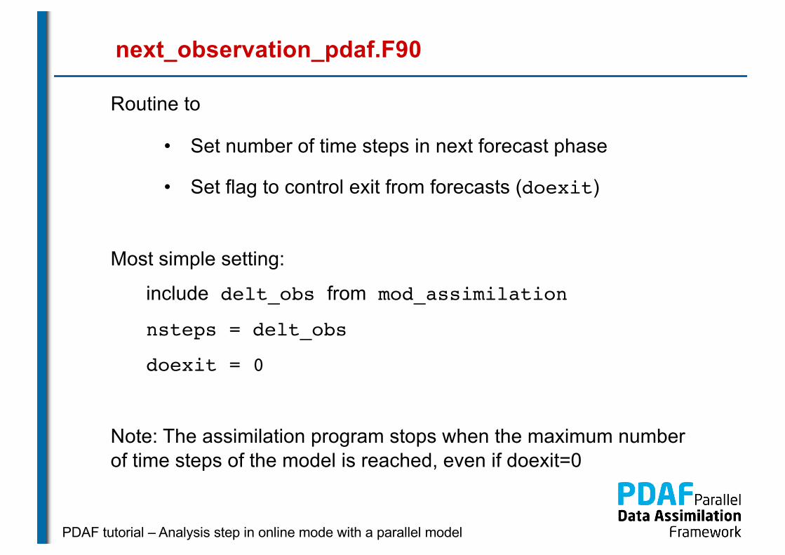
next_observation_pdaf.F90
Routine to
• Set number of time steps in next forecast phase
• Set flag to control exit from forecasts (doexit)
Most simple setting:
include delt_obs from mod_assimilation
nsteps = delt_obs
doexit = 0
Note: The assimilation program stops when the maximum number of time steps of the model is reached, even if doexit=0
PDAF tutorial – Analysis step in online mode with a parallel model
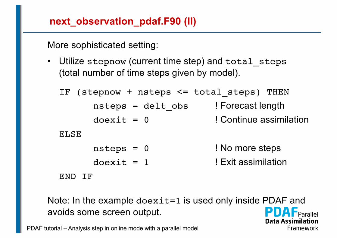
next_observation_pdaf.F90 (II)
More sophisticated setting:
• Utilize stepnow (current time step) and total_steps(total number of time steps given by model).
IF (stepnow + nsteps <= total_steps) THENnsteps = delt_obs ! Forecast length
doexit = 0 ! Continue assimilation
ELSEnsteps = 0 ! No more steps
doexit = 1 ! Exit assimilation
END IF
Note: In the example doexit=1 is used only inside PDAF and avoids some screen output.

PDAF tutorial – Analysis step in online mode with a parallel model
distribute_state_pdaf.F90
Routine to
• Initialize model fields from a state vector
• Routine is provided with the state vector vector_p
For the example:
1. Access nx_p, ny and field_p with use mod_model
2. Initialize model field from state vector:
DO j = 1, nx_p
field_p(1:ny, j) = state_p(1+(j-1)*ny : j*ny)
END DO
PDAF tutorial – Analysis step in online mode with a parallel model
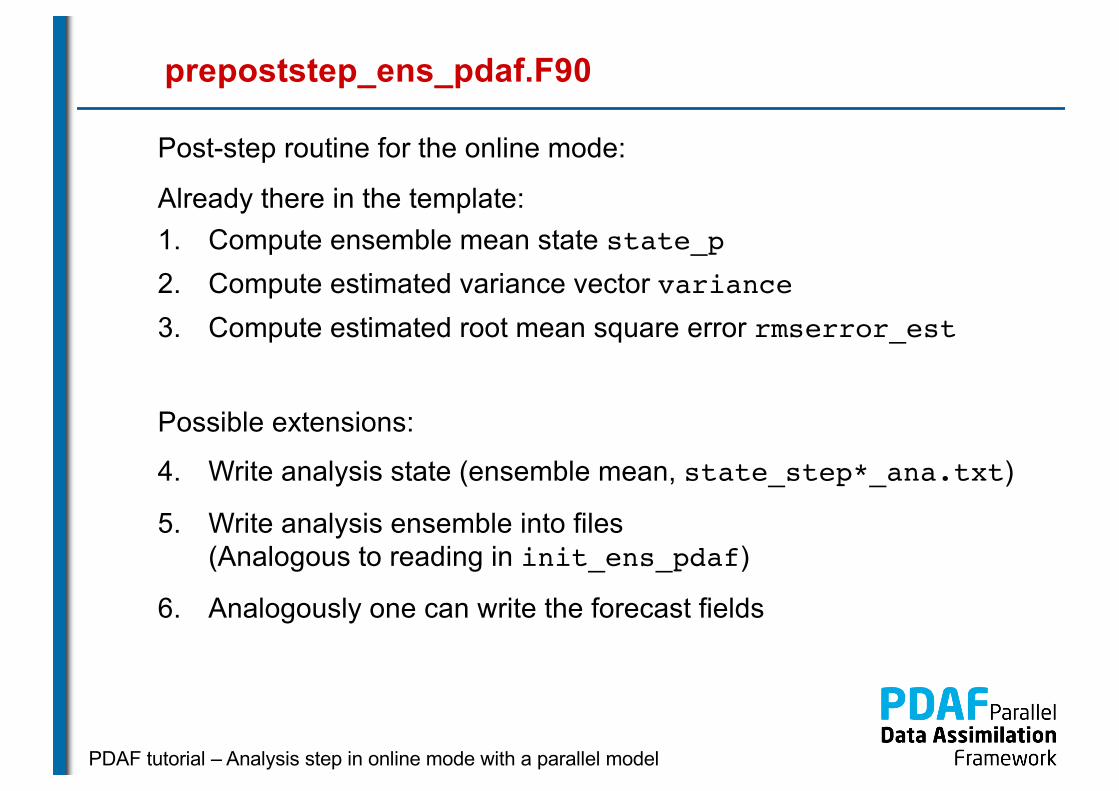
prepoststep_ens_pdaf.F90
Post-step routine for the online mode:
Already there in the template:1. Compute ensemble mean state state_p2. Compute estimated variance vector variance3. Compute estimated root mean square error rmserror_est
Possible extensions:
4. Write analysis state (ensemble mean, state_step*_ana.txt)
5. Write analysis ensemble into files (Analogous to reading in init_ens_pdaf)
6. Analogously one can write the forecast fields
PDAF tutorial – Analysis step in online mode with a parallel model
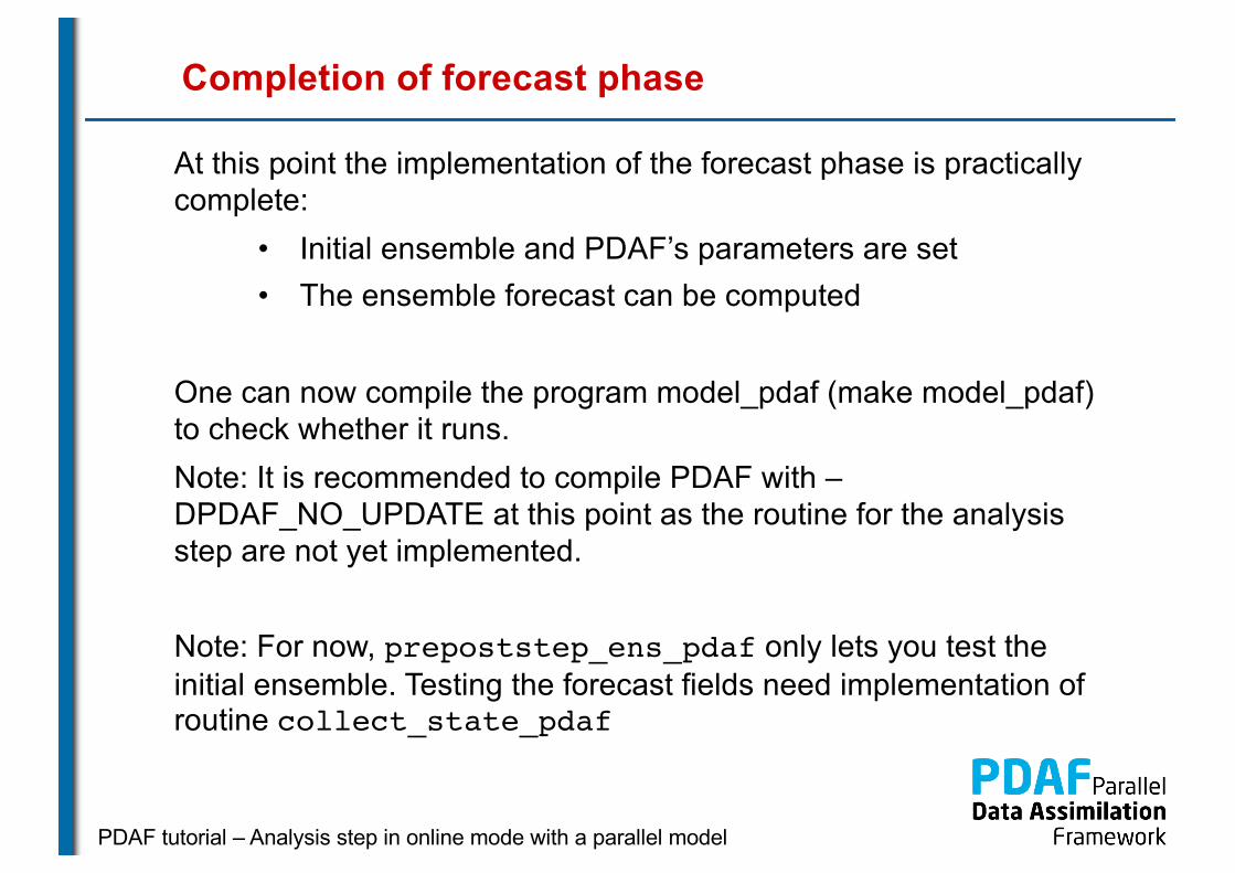
Completion of forecast phase
At this point the implementation of the forecast phase is practically complete:
• Initial ensemble and PDAF’s parameters are set• The ensemble forecast can be computed
One can now compile the program model_pdaf (make model_pdaf) to check whether it runs. Note: It is recommended to compile PDAF with –DPDAF_NO_UPDATE at this point as the routine for the analysis step are not yet implemented.
Note: For now, prepoststep_ens_pdaf only lets you test the initial ensemble. Testing the forecast fields need implementation of routine collect_state_pdaf
PDAF tutorial – Analysis step in online mode with a parallel model
1a) Global filter
PDAF tutorial – Analysis step in online mode with a parallel model
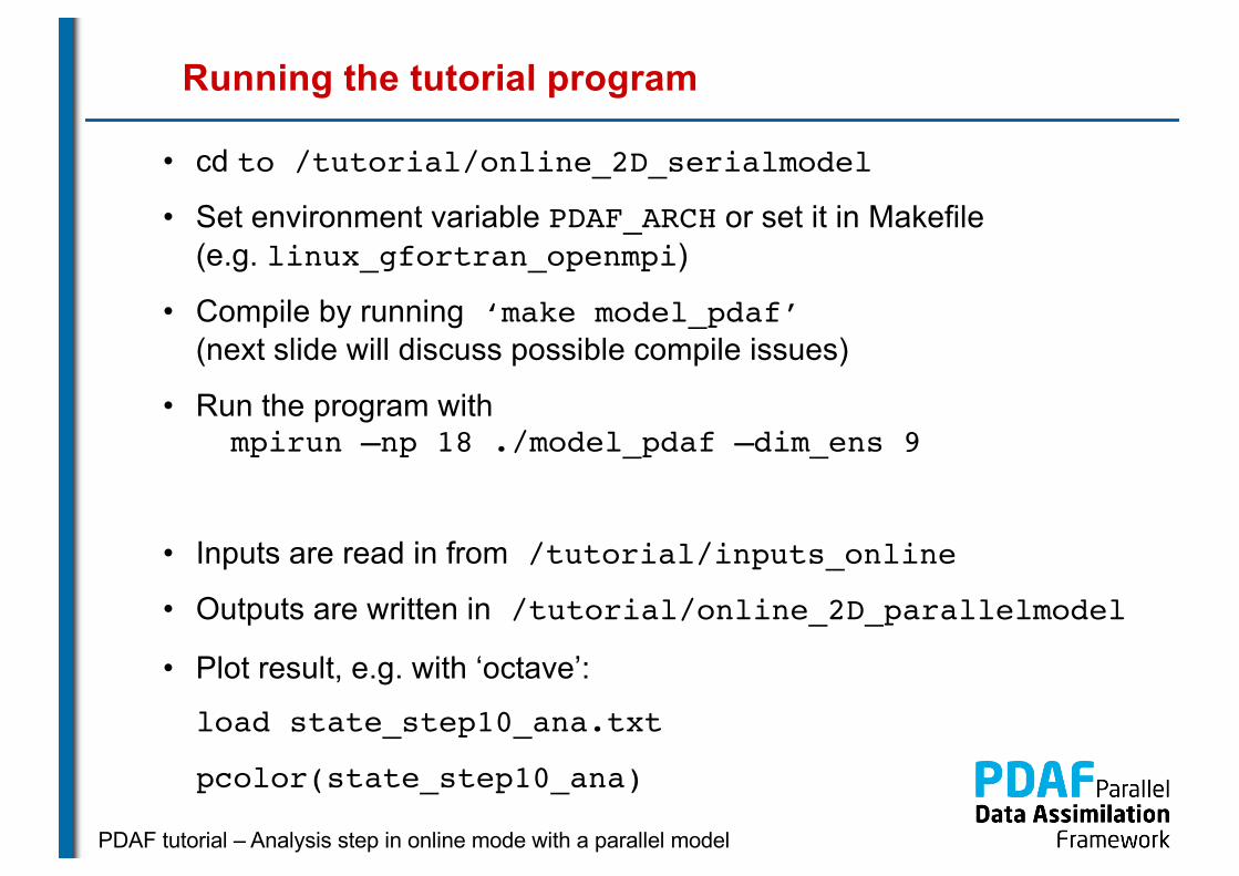
Running the tutorial program
• cd to /tutorial/online_2D_serialmodel
• Set environment variable PDAF_ARCH or set it in Makefile
(e.g. linux_gfortran_openmpi)
• Compile by running ‘make model_pdaf’(next slide will discuss possible compile issues)
• Run the program with
mpirun –np 18 ./model_pdaf –dim_ens 9
• Inputs are read in from /tutorial/inputs_online
• Outputs are written in /tutorial/online_2D_parallelmodel
• Plot result, e.g. with ‘octave’:
load state_step10_ana.txt
pcolor(state_step10_ana)
PDAF tutorial – Analysis step in online mode with a parallel model
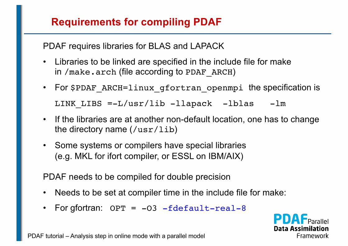
Requirements for compiling PDAF
PDAF requires libraries for BLAS and LAPACK
• Libraries to be linked are specified in the include file for make in /make.arch (file according to PDAF_ARCH)
• For $PDAF_ARCH=linux_gfortran_openmpi the specification is
LINK_LIBS =-L/usr/lib -llapack -lblas -lm
• If the libraries are at another non-default location, one has to change the directory name (/usr/lib)
• Some systems or compilers have special libraries (e.g. MKL for ifort compiler, or ESSL on IBM/AIX)
PDAF needs to be compiled for double precision
• Needs to be set at compiler time in the include file for make:
• For gfortran: OPT = -O3 -fdefault-real-8
PDAF tutorial – Analysis step in online mode with a parallel model
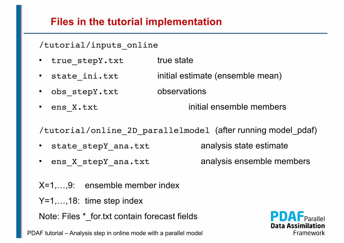
Files in the tutorial implementation
/tutorial/inputs_online
• true_stepY.txt true state
• state_ini.txt initial estimate (ensemble mean)
• obs_stepY.txt observations
• ens_X.txt initial ensemble members
/tutorial/online_2D_parallelmodel (after running model_pdaf)
• state_stepY_ana.txt analysis state estimate
• ens_X_stepY_ana.txt analysis ensemble members
X=1,…,9: ensemble member index
Y=1,…,18: time step index
Note: Files *_for.txt contain forecast fields

PDAF tutorial – Analysis step in online mode with a parallel model
Result of the global assimilation
For example, at step 10
• The analysis state (center) is closer to the true field than without assimilation (left)
• Truth and analysis are nearly identical (right)
PDAF tutorial – Analysis step in online mode with a parallel model
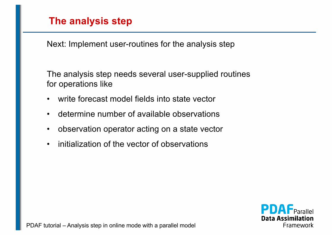
The analysis step
Next: Implement user-routines for the analysis step
The analysis step needs several user-supplied routinesfor operations like
• write forecast model fields into state vector
• determine number of available observations
• observation operator acting on a state vector
• initialization of the vector of observations
PDAF tutorial – Analysis step in online mode with a parallel model
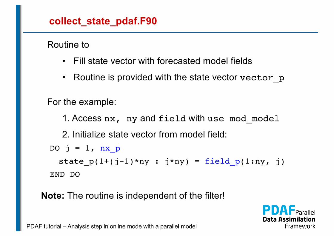
collect_state_pdaf.F90
Routine to
• Fill state vector with forecasted model fields
• Routine is provided with the state vector vector_p
For the example:
1. Access nx, ny and field with use mod_model
2. Initialize state vector from model field:DO j = 1, nx_pstate_p(1+(j-1)*ny : j*ny) = field_p(1:ny, j)
END DO
Note: The routine is independent of the filter!
PDAF tutorial – Analysis step in online mode with a parallel model
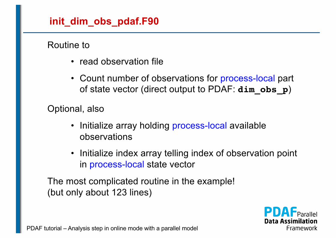
init_dim_obs_pdaf.F90
Routine to
• read observation file
• Count number of observations for process-local part of state vector (direct output to PDAF: dim_obs_p)
Optional, also
• Initialize array holding process-local available observations
• Initialize index array telling index of observation point in process-local state vector
The most complicated routine in the example!(but only about 123 lines)
PDAF tutorial – Analysis step in online mode with a parallel model
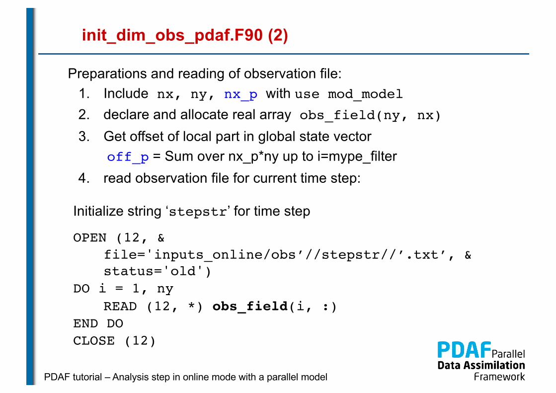
init_dim_obs_pdaf.F90 (2)
Preparations and reading of observation file:1. Include nx, ny, nx_p with use mod_model2. declare and allocate real array obs_field(ny, nx)3. Get offset of local part in global state vector
off_p = Sum over nx_p*ny up to i=mype_filter4. read observation file for current time step:
Initialize string ‘stepstr’ for time step
OPEN (12, &file='inputs_online/obs’//stepstr//’.txt’, &status='old')
DO i = 1, nyREAD (12, *) obs_field(i, :)
END DOCLOSE (12)
PDAF tutorial – Analysis step in online mode with a parallel model
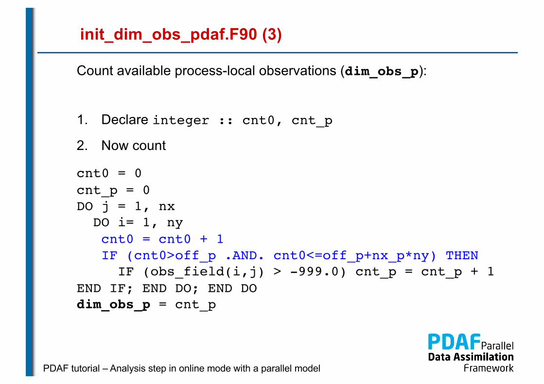
init_dim_obs_pdaf.F90 (3)
Count available process-local observations (dim_obs_p):
1. Declare integer :: cnt0, cnt_p
2. Now count
cnt0 = 0cnt_p = 0DO j = 1, nx
DO i= 1, nycnt0 = cnt0 + 1 IF (cnt0>off_p .AND. cnt0<=off_p+nx_p*ny) THEN
IF (obs_field(i,j) > -999.0) cnt_p = cnt_p + 1END IF; END DO; END DOdim_obs_p = cnt_p
PDAF tutorial – Analysis step in online mode with a parallel model
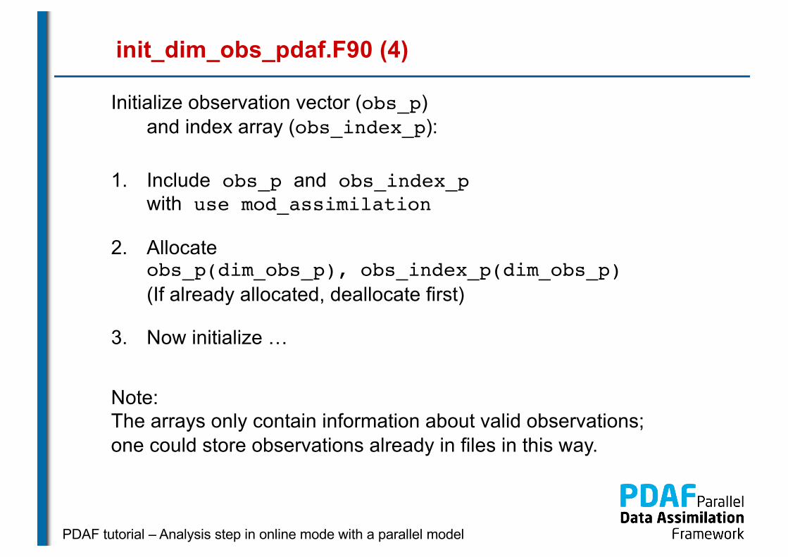
init_dim_obs_pdaf.F90 (4)
Initialize observation vector (obs_p) and index array (obs_index_p):
1. Include obs_p and obs_index_pwith use mod_assimilation
2. Allocate obs_p(dim_obs_p), obs_index_p(dim_obs_p)(If already allocated, deallocate first)
3. Now initialize …
Note: The arrays only contain information about valid observations; one could store observations already in files in this way.

PDAF tutorial – Analysis step in online mode with a parallel model
init_dim_obs_pdaf.F90 (5)
Initialize obs and obs_index
cnt0 = cnt_p = cnt0_p = 0 ! Count grid pointsDO j = 1, nx
DO i= 1, nycnt0 = cnt0 + 1IF (cnt0>off_p .AND. &
cnt0<=off_p+nx_p*ny) THENcnt0_p = cnt0_p + 1
IF (obs_field(i,j) > -999.0) THENcnt_p = cnt_p + 1obs_index_p(cnt_p) = cnt0_p ! Indexobs_p(cnt_p) = obs_field(i, j) ! observations
END IF; END IFEND DO
END DO

PDAF tutorial – Analysis step in online mode with a parallel model
obs_op_pdaf.F90
Implementation of observation operator acting one some state vector
Input: state vector state_p
Output: observed state vector m_state_p
1. Include obs_index_p by use mod_assimilation
2. Select observed grid points from state vector:
DO i = 1, dim_obs_pm_state_p(i) = state_p(obs_index_p(i))
END DO
Note:dim_obs_p is an input argument of the routine

PDAF tutorial – Analysis step in online mode with a parallel model
init_obs_pdaf.F90
Fill PDAF’s observation vector
Output: vector of observations observation_p
1. Include obs_p with use mod_assimilation
2. Initialize observation_p:
observation_p = obs_p
Note:This is trivial, because of the preparations in init_dim_obs_pdaf!(However, the operations needed to be separate, because PDAF allocates observations_p after the call to init_dim_obs_pdaf)

PDAF tutorial – Analysis step in online mode with a parallel model
prodrinva_pdaf.F90
Compute the product of the inverse observation error covariance matrix with some other matrix
• Input: Matrix A_p(dim_obs_p, rank)• Output: Product matrix C_p(dim_obs_p, rank)
(rank is typically dim_ens-1)
1. Declare and initialize inverse observation error variance ivariance_obs = 1.0 / rms_obs**2
2. Compute product:
DO j = 1, rankDO i = 1, dim_obs_p
C_p(i, j) = ivariance_obs * A_p(i, j)END DO
END DO
PDAF tutorial – Analysis step in online mode with a parallel model
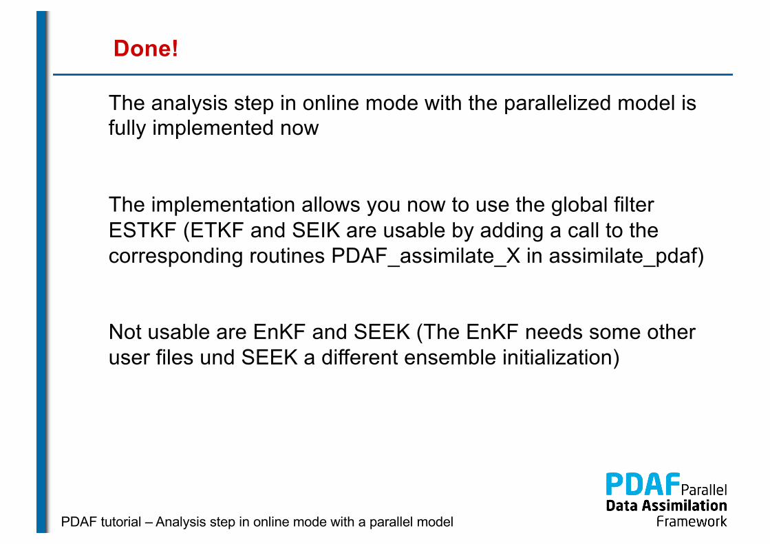
Done!
The analysis step in online mode with the parallelized model is fully implemented now
The implementation allows you now to use the global filter ESTKF (ETKF and SEIK are usable by adding a call to the corresponding routines PDAF_assimilate_X in assimilate_pdaf)
Not usable are EnKF and SEEK (The EnKF needs some other user files und SEEK a different ensemble initialization)

PDAF tutorial – Analysis step in online mode with a parallel model
A complete analysis step
We now have a fully functional analysis step
- if no localization is required!
Possible extensions for a real application:
Adapt routines for
Ø Multiple model fields
➜ Store full fields consecutively in state vector
Ø Third dimension
➜ Extend state vector
Ø Different observation types
➜ Store different types consecutively in observation vector
Ø Other file type (e.g. binary or NetCDF)
➜ Adapt reading/writing routines

PDAF tutorial – Analysis step in online mode with a parallel model
Differences between online and offline modes
For the analysis step in online mode:
collect_state_pdaf - additional routine for online mode
init_dim_obs_pdaf - read from file for current time step; include nx, ny from mod_model
instead of mod_assimilate
obs_op_pdaf - identical in online and offline modes
init_obs_pdaf - identical in online and offline modes
prodrinva_pdaf - identical in online and offline modes
PDAF tutorial – Analysis step in online mode with a parallel model
1b) Local filter with parallelized model

PDAF tutorial – Analysis step in online mode with a parallel model
Localization
Localization is usually required for high-dimensional systems
• Update small regions (S)(e.g. single grid points, single vertical columns)
• Consider only observations within cut-off distance (D)
• Weight observations according to distance from S
PDAF tutorial – Analysis step in online mode with a parallel model
The FULL observation vector
• A single local analysis at S (single grid point) need observations
from domain D
• A loop of local analyses over all S needs all observations
• This defines the full observation vector
• Why distinguish full and all observations?
➜ They can be different in case of parallelization!
• Example:
Ø Split domain in left and right halves
Ø Some of the analyses in left half
need observations from the right side.
Ø Depending on localization radius not all observations from
the right side might be needed for the left side analyses
PDAF tutorial – Analysis step in online mode with a parallel model
Running the tutorial program
• Compile as for the global filter• Run the program with
mpirun –np 18 ./model_pdaf –dim_ens 9 OPTIONS
• OPTIONS are always of type –KEYWORD VALUE• Possible OPTIONS are
-filtertype 7 (select LESTKF if not set in init_pdaf)-local_range 5.0 (set localization radius, 0.0 by default, any
positive value should work)-locweight 2 (set weight function for localization, default=0
for constant weight of 1; possible are integer values 0 to 4; see init_pdaf)
Note: You can run the model e.g. using 18 MPI-processes even on most computers with only 2 processor cores. However, to see a speedup in computing time, you need more physical processors

PDAF tutorial – Analysis step in online mode with a parallel model
Result of the local assimilation
mpirun –np 9./model_pdaf –dim_ens 9 -filtertype 7
• Default: zero localization radius (local_range=0.0)
• Change only at observation locations

PDAF tutorial – Analysis step in online mode with a parallel model
Result of the local assimilation (2)
… -filtertype 7 -local_range 10.0
• All local analysis domains are influenced (all see observations)
• Up to 16 observations in a single local analysis (average 9.6)
Note: The set up of the experiment favors the global filter because of the shape of the ensemble members
PDAF tutorial – Analysis step in online mode with a parallel model
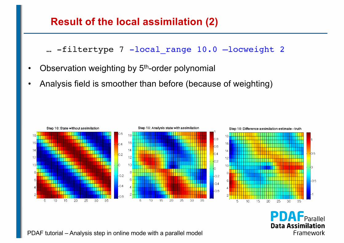
Result of the local assimilation (2)
… -filtertype 7 -local_range 10.0 –locweight 2
• Observation weighting by 5th-order polynomial
• Analysis field is smoother than before (because of weighting)
PDAF tutorial – Analysis step in online mode with a parallel model
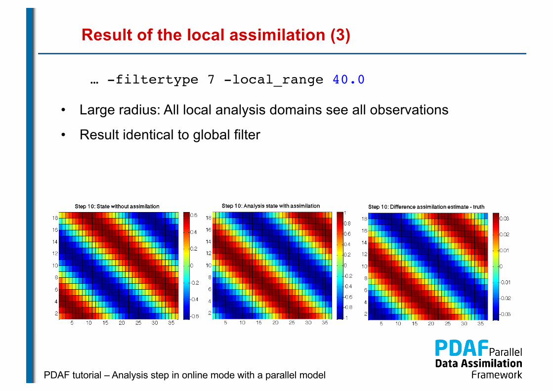
Result of the local assimilation (3)
… -filtertype 7 -local_range 40.0
• Large radius: All local analysis domains see all observations
• Result identical to global filter
PDAF tutorial – Analysis step in online mode with a parallel model
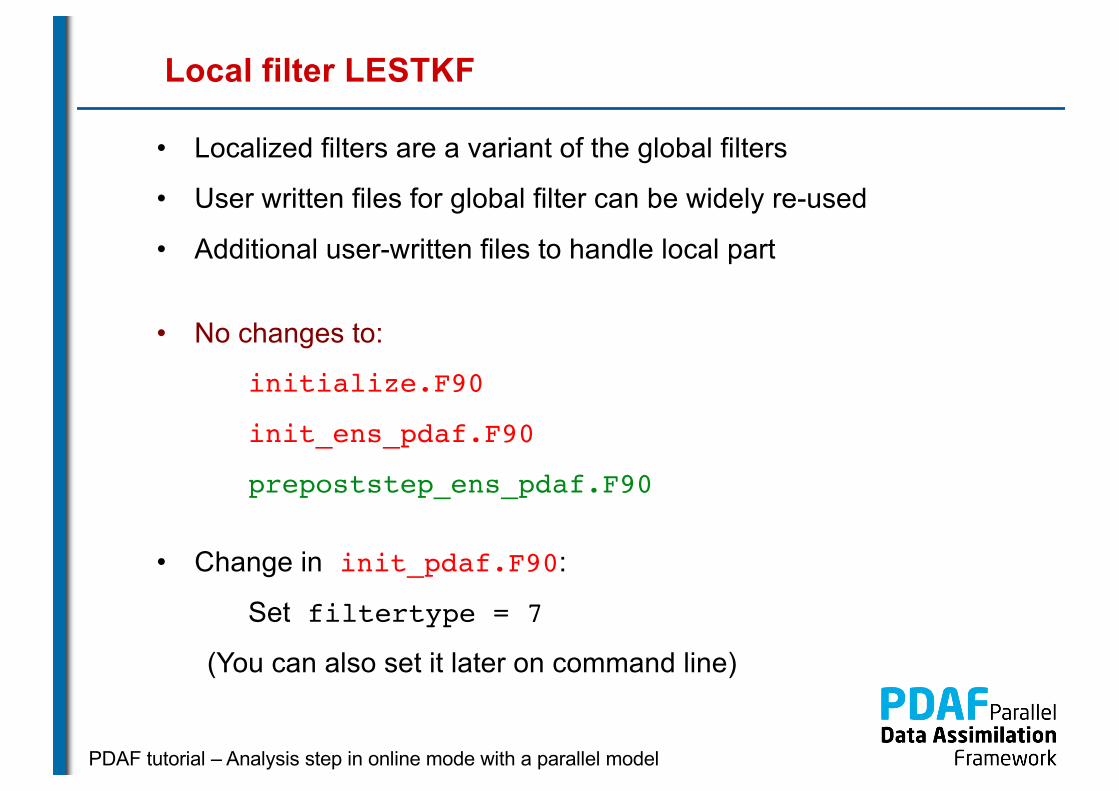
Local filter LESTKF
• Localized filters are a variant of the global filters
• User written files for global filter can be widely re-used
• Additional user-written files to handle local part
• No changes to:
initialize.F90
init_ens_pdaf.F90
prepoststep_ens_pdaf.F90
• Change in init_pdaf.F90:
Set filtertype = 7
(You can also set it later on command line)

PDAF tutorial – Analysis step in online mode with a parallel model
Local filter LESTKF (2)
Adapt files from global analysis
init_dim_obs_pdaf.F90 � init_dim_obs_f_pdaf.F90obs_op_pdaf.F90 � obs_op_f_pdaf.F90init_obs_pdaf.F90 � init_obs_f_pdaf.F90prodrinva_pdaf.F90 � prodrinva_l_pdaf
Naming scheme:
_f_ “full”: operate on all required observations (without parallelization these are all observations)
_l_ “local”: operation in local analysis domain or correspondinglocal observation domain

PDAF tutorial – Analysis step in online mode with a parallel model
Local filter LESTKF (3)
Additional files for local analysis step
init_n_domains_pdaf.F90init_dim_l_pdaf.F90init_dim_obs_l_pdaf.F90g2l_state_pdaf.F90g2l_obs_pdaf.F90init_obs_l_pdaf.F90l2g_state_pdaf.F90
Discuss now the files in the order they are called
PDAF tutorial – Analysis step in online mode with a parallel model
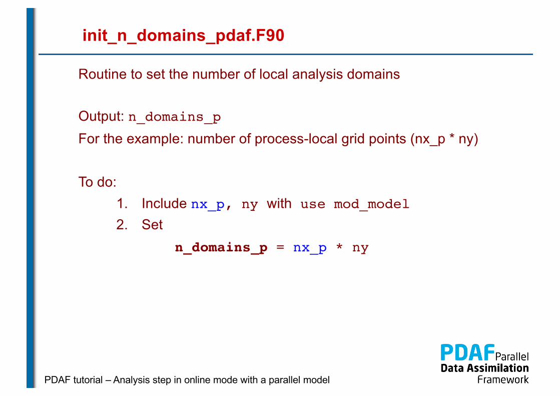
init_n_domains_pdaf.F90
Routine to set the number of local analysis domains
Output: n_domains_pFor the example: number of process-local grid points (nx_p * ny)
To do:1. Include nx_p, ny with use mod_model2. Set
n_domains_p = nx_p * ny
PDAF tutorial – Analysis step in online mode with a parallel model
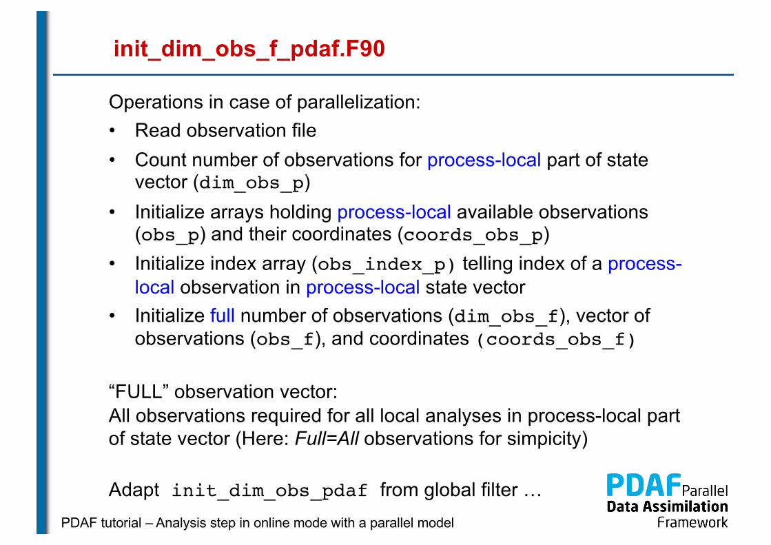
init_dim_obs_f_pdaf.F90
Operations in case of parallelization:• Read observation file• Count number of observations for process-local part of state
vector (dim_obs_p)• Initialize arrays holding process-local available observations
(obs_p) and their coordinates (coords_obs_p)• Initialize index array (obs_index_p) telling index of a process-
local observation in process-local state vector• Initialize full number of observations (dim_obs_f), vector of
observations (obs_f), and coordinates (coords_obs_f)
“FULL” observation vector:All observations required for all local analyses in process-local part of state vector (Here: Full=All observations for simpicity)
Adapt init_dim_obs_pdaf from global filter …
PDAF tutorial – Analysis step in online mode with a parallel model
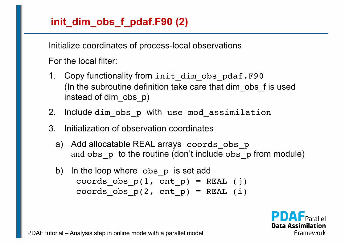
init_dim_obs_f_pdaf.F90 (2)
Initialize coordinates of process-local observations
For the local filter:
1. Copy functionality from init_dim_obs_pdaf.F90(In the subroutine definition take care that dim_obs_f is used instead of dim_obs_p)
2. Include dim_obs_p with use mod_assimilation
3. Initialization of observation coordinates
a) Add allocatable REAL arrays coords_obs_pand obs_p to the routine (don’t include obs_p from module)
b) In the loop where obs_p is set addcoords_obs_p(1, cnt_p) = REAL (j)coords_obs_p(2, cnt_p) = REAL (i)
PDAF tutorial – Analysis step in online mode with a parallel model
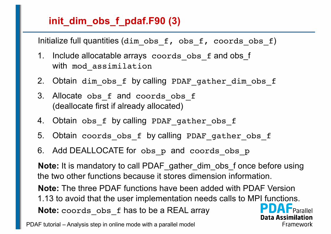
init_dim_obs_f_pdaf.F90 (3)
Initialize full quantities (dim_obs_f, obs_f, coords_obs_f)
1. Include allocatable arrays coords_obs_f and obs_fwith mod_assimilation
2. Obtain dim_obs_f by calling PDAF_gather_dim_obs_f
3. Allocate obs_f and coords_obs_f(deallocate first if already allocated)
4. Obtain obs_f by calling PDAF_gather_obs_f
5. Obtain coords_obs_f by calling PDAF_gather_obs_f
6. Add DEALLOCATE for obs_p and coords_obs_p
Note: It is mandatory to call PDAF_gather_dim_obs_f once before using the two other functions because it stores dimension information.Note: The three PDAF functions have been added with PDAF Version 1.13 to avoid that the user implementation needs calls to MPI functions.Note: coords_obs_f has to be a REAL array
PDAF tutorial – Analysis step in online mode with a parallel model
obs_op_f_pdaf.F90
Implementation of observation operator for full observation domain
Difficulty:
• The state vector state_p is local to each process
• Full observed vector goes beyond process boundary
Implement two steps:
1. Initialize process-local observed state
2. Gather full observed state vector using MPI
PDAF tutorial – Analysis step in online mode with a parallel model
obs_op_f_pdaf.F90 (2)
1. Initialize process-local observed state m_state_p
a) Include dim_obs_p and obs_index_pwith use mod_assimilation
b) Declare real allocatable array m_state_p(:)
c) Allocate m_state_p(dim_obs_p)
d) Fill the array
DO i = 1, dim_obs_pm_state_p(i) = state_p(obs_index_p(i))
END DO
PDAF tutorial – Analysis step in online mode with a parallel model
obs_op_f_pdaf.F90 (3)
2. Get full observed state vector
a) Add variable INTEGER :: status
b) Add call to PDAF_gather_obs_f:
CALL PDAF_gather_obs_f(m_state_p, m_state_f, status)
c) Deallocate m_state_p
Note: It is mandatory to call PDAF_gather_dim_obs_f once before using the two other functions because it stores dimension information. Usually this was already done in init_dim_obs_f_pdaf
PDAF tutorial – Analysis step in online mode with a parallel model
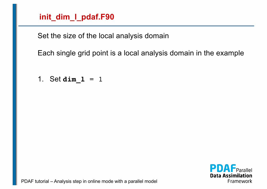
init_dim_l_pdaf.F90
Set the size of the local analysis domain
Each single grid point is a local analysis domain in the example
1. Set dim_l = 1
PDAF tutorial – Analysis step in online mode with a parallel model
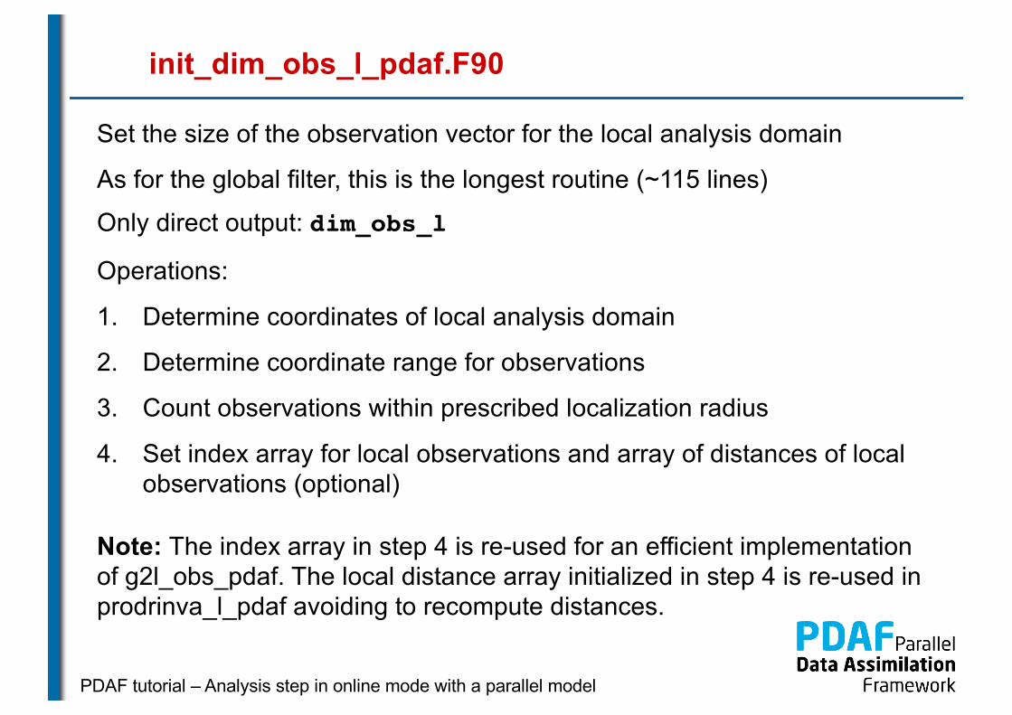
init_dim_obs_l_pdaf.F90
Set the size of the observation vector for the local analysis domain
As for the global filter, this is the longest routine (~115 lines)
Only direct output: dim_obs_l
Operations:
1. Determine coordinates of local analysis domain
2. Determine coordinate range for observations
3. Count observations within prescribed localization radius
4. Set index array for local observations and array of distances of local observations (optional)
Note: The index array in step 4 is re-used for an efficient implementation of g2l_obs_pdaf. The local distance array initialized in step 4 is re-used in prodrinva_l_pdaf avoiding to recompute distances.

PDAF tutorial – Analysis step in online mode with a parallel model
init_dim_obs_l_pdaf.F90 (2)
1. Determine coordinates of local analysis domain
1. Compute offset:
off_p = Sum over nx_p*ny up to i=mype_filter
2. Declare real :: coords_l(2)
3. Include nx, ny, nx_p with use mod_model
4. Compute coords_l from nx, ny:
coords_l(1) = real(ceiling(real(domain_p + off_p)/real(ny)))
coords_l(2) = real(domain_p + off_p) - (coords_l(1)-1)*ny
Note: With parallelization the domain numbering begins with 1 for each process. For the coordinates we also need to count the domains from processes with lower process rank using off_p

PDAF tutorial – Analysis step in online mode with a parallel model
init_dim_obs_l_pdaf.F90 (3)
2. Determine coordinate range for local observations
1. Declare real :: limits_x(2), limits_y(2)2. Include local_range with use mod_assimilation3. Set lower and upper limits. E.g. for x-direction
limits_x(1) = coords_l(1) - local_rangeif (limits_x(1) < 1.0) limits_x(1) = 1.0limits_x(2) = coords_l(1) + local_rangeif (limits_x(2) > real(nx)) limits_x(2) = real(nx)
(analogous for y-direction)
Note: Using limits_x, limits_y is not strictly required, but it makes the search for local observations more efficient.If the localization is only based on grid point indices, the coordinates could be handled as integer values

PDAF tutorial – Analysis step in online mode with a parallel model
init_dim_obs_l_pdaf.F90 (4)
3. Count local observations (within distance local_range)dim_obs_l = 0
DO i = 1, dim_obs_f
IF (“coords_obs_f(:,i) within coordinate limits”) THENCompute distance between coords_obs and coords_l
IF (distance <= local_range) &
dim_obs_l = dim_obs_l + 1
END IF
END DO
Note:For efficiency, we only compute distance for observations within coordinate limits limits_x, limits_y. Valid local observations reside within circle of radius local_range.
PDAF tutorial – Analysis step in online mode with a parallel model
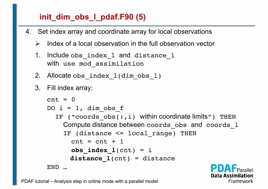
init_dim_obs_l_pdaf.F90 (5)
4. Set index array and coordinate array for local observations
Ø Index of a local observation in the full observation vector
1. Include obs_index_l and distance_lwith use mod_assimilation
2. Allocate obs_index_l(dim_obs_l)
3. Fill index array:
cnt = 0DO i = 1, dim_obs_f
IF (“coords_obs(:,i) within coordinate limits”) THENCompute distance between coords_obs and coords_lIF (distance <= local_range) THEN
cnt = cnt + 1obs_index_l(cnt) = idistance_l(cnt) = distance
END …

PDAF tutorial – Analysis step in online mode with a parallel model
g2l_state_pdaf.F90
Initialize state vector for local analysis domain from global state vector
Ø Here the local state is just one element of the global state vector
Input: state_p(1:dim_p)
Output: state_l(1:dim_l)
1. Setstate_l = state_p(domain_p)
Note:dim_l = 1 in the example
PDAF tutorial – Analysis step in online mode with a parallel model
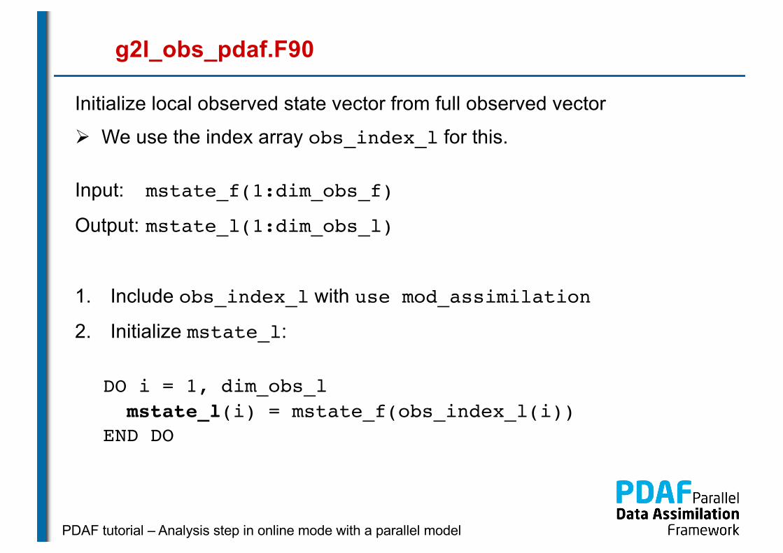
g2l_obs_pdaf.F90
Initialize local observed state vector from full observed vector
Ø We use the index array obs_index_l for this.
Input: mstate_f(1:dim_obs_f)
Output: mstate_l(1:dim_obs_l)
1. Include obs_index_l with use mod_assimilation
2. Initialize mstate_l:
DO i = 1, dim_obs_lmstate_l(i) = mstate_f(obs_index_l(i))
END DO
PDAF tutorial – Analysis step in online mode with a parallel model
init_obs_l_pdaf.F90
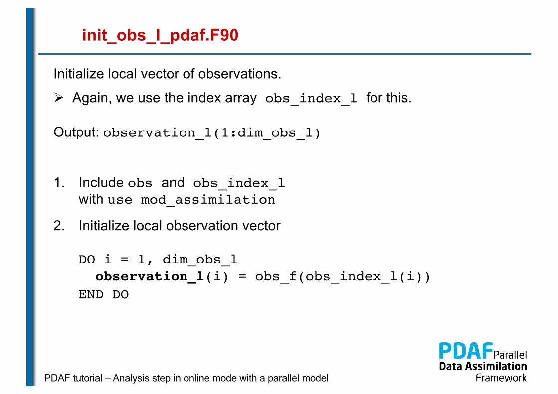
Initialize local vector of observations.
Ø Again, we use the index array obs_index_l for this.
Output: observation_l(1:dim_obs_l)
1. Include obs and obs_index_lwith use mod_assimilation
2. Initialize local observation vector
DO i = 1, dim_obs_lobservation_l(i) = obs_f(obs_index_l(i))
END DO

PDAF tutorial – Analysis step in online mode with a parallel model
prodrinva_l_pdaf.F90
Compute the product of the inverse observation error covariance matrix with some other matrix+ apply observation localization (weighting)
Ø The weighting and the product are fully implemented for a diagonal observation error covariance matrix with constant variance
When we re-use the array distance_l initialized in init_dim_obs_l_pdaf, no changes are required here.

PDAF tutorial – Analysis step in online mode with a parallel model
l2g_state_pdaf.F90
Initialize global state vector from state vector for local analysis domain
Ø Here the local state is just one element of the global state vector
Input: state_l(1:dim_l)
Output: state_p(1:dim_p)
1. Implement inverse operation to that in g2l_state_pdaf.F90
state_p(domain_p) = state_l
Note: The implementation utilizes that dim_l = 1

PDAF tutorial – Analysis step in online mode with a parallel model
Done!
Now, the analysis step for local ESKTF in offline mode is fully implemented.
The implementation allows you now to use the local filter LESTKF (LETKF, LSEIK can be used after adding calls to PDAF_assimilate_X)
Not usable are EnKF and SEEK (PDAF does not have localization for these filters)
For testing one can vary localization parameters:
local_range – the localization radius
locweight – the weighting method
Default are local_range=0.0 (observation at single grid point) and locweight=1 (uniform weight)
PDAF tutorial – Analysis step in online mode with a serial model
2) Hints for adaptions for real models

PDAF tutorial – Analysis step in online mode with a parallel model
Implementations for real models
• Tutorial demonstrates implementation for simple model
• You can base your own implementation on the tutorial implementation or the templates provided with PDAF
• Need to adapt most routines, e.g.
• Specify model-specific state vector and its dimension
• Adapt distribute_state and collect_state
• Adapt routines handling observations
• Further required changes
• Adapt file output (usually only want to write ensemble mean state in prepoststep_pdaf; sometimes possible to use output routines from model)
PDAF tutorial – Analysis step in online mode with a parallel model
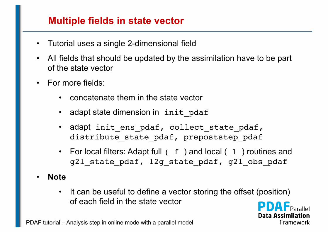
Multiple fields in state vector
• Tutorial uses a single 2-dimensional field
• All fields that should be updated by the assimilation have to be part of the state vector
• For more fields:
• concatenate them in the state vector
• adapt state dimension in init_pdaf
• adapt init_ens_pdaf, collect_state_pdaf, distribute_state_pdaf, prepoststep_pdaf
• For local filters: Adapt full (_f_) and local (_l_) routines and g2l_state_pdaf, l2g_state_pdaf, g2l_obs_pdaf
• Note
• It can be useful to define a vector storing the offset (position) of each field in the state vector
PDAF tutorial – Analysis step in online mode with a parallel model
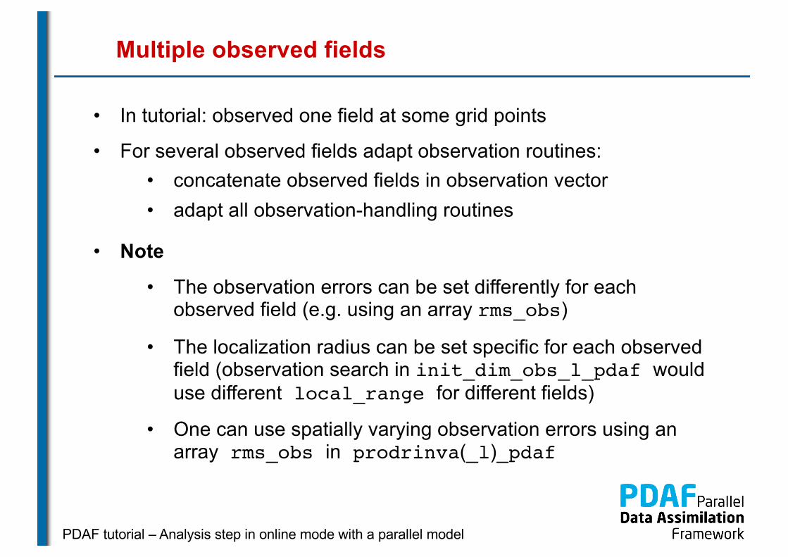
Multiple observed fields
• In tutorial: observed one field at some grid points
• For several observed fields adapt observation routines:• concatenate observed fields in observation vector• adapt all observation-handling routines
• Note
• The observation errors can be set differently for each observed field (e.g. using an array rms_obs)
• The localization radius can be set specific for each observed field (observation search in init_dim_obs_l_pdaf would use different local_range for different fields)
• One can use spatially varying observation errors using an array rms_obs in prodrinva(_l)_pdaf
PDAF tutorial – Analysis step in online mode with a parallel model
The End!
Tutorial described example implementations
• Online mode of PDAF
• Simple 2D model with parallelization
• Parallelization over ensemble members at the model itself
• Square root filter ESTKF
• global and with localization
• Extension to more realistic cases possible with limited coding
• Applicable also for large-scale problems
For full documentation of PDAF and the user-implemented routines
see http://pdaf.awi.de