PCRD-R-4 What Is Rural and What Is Urban in Indiana? · publication explains the commonly used rural/urban classifications and what ... What Is Rural and What Is Urban in Indiana?

PCRD-R-4

Brigitte S. Waldorf

Department of Agricultural Economics

Purdue University

West Lafayette, Indiana

To the PointWhat is urban and what is rural is a topic of continuing debate. This

publication explains the commonly used rural/urban classifications and what they mean for Indiana. It argues that these classifications suffer from serious shortcomings, most notably the “threshold trap,” which in the extreme is an “all or nothing” grouping. As an alternative, this report introduces the Index of Relative Rurality. The index shifts emphasis away from often ill-defined categories of rural and urban. Instead of answering the question “Is it rural, or not?” it answers the question “How rural is it?” As such, the Index of Relative Rurality promises to shed new light on issues ranging from rural poverty to economic growth in urban and rural areas.

Regional Development for Local Success

What Is Rural and What Is Urban in Indiana?

Purdue Center for Regional Development

CRDP

IntroductionDid you know that Ohio County in Southeastern Indiana is as “urban” as

Marion County? Even more surprising, it is as “urban” as the most densely populated counties of the East Coast megalopolis. This is true at least when using the so-called “rural-urban continuum code” that was developed by USDA/ERS.

The rural-urban continuum code is just one of many schemes used to categorize U.S. counties and give shape to the important yet vague concept of rurality. Other schemes include the urban/rural distinction defined by the U.S. Census Bureau; the metropolitan, micropolitan, and noncore county classification of the Office of Management and Budget; and the rural-urban density typology recently introduced by Andrew Isserman.

Why does having a good definition of rurality matter? Although rurality is a vague concept that defies a straightforward definition, policy makers need a clear delineation of rurality when designing policies and development strategies. The problem is that, depending on the classification scheme used, a county may or may not be a beneficiary of rural policies. An example is the recently published strategic plan for rural Indiana (RISE 2020), which starts with the very important decision to define rural Indiana as the group of “non-metropolitan counties.” This decision implies, for example, that Benton County, with its low population density and small population size, is not part of rural Indiana as defined in RISE 2020 because it belongs to the Lafayette Metropolitan Area.

This report pursues two aims. First, it explains the commonly used schemes to distinguish between rural and urban. A critical evaluation of these schemes


�

shows that they use somewhat arbitrary thresholds to distinguish between rural and urban places and thus fall into the “threshold trap.” The report places special emphasis on what this means for the classification of Indiana counties.

Second, the report introduces a new measure of rurality, the Index of Relative Rurality. This index assesses counties’ degree of rurality on a continuous scale and thus does not rely on arbitrary thresholds. Mapping the Index of Relative Rurality shows that—compared to the nation as a whole—most Indiana counties have a medium level of rurality. Extreme rurality is absent from Indiana. Finally, the report also outlines the advantages of the new index when designing development policies.

Classification Scheme I: Urban Areas as Defined by the U.S. Census Bureau

The U.S. Census Bureau does not categorize counties as urban or rural. Instead, it defines urban areas on the basis of census blocks. An urban area can thus include an entire county or parts of a county. More precisely, an urban area is a contiguous area of census blocks or block groups that has, at its core, a population density of at least 1,000 persons per square mile and a total population of 2,500 or more residents.1 Two types of urban areas are distinguished: urbanized areas and urban clusters (Figure 1).

• An urbanized area has at least 50,000 residents.

• An urban cluster has at least 2,500 residents but fewer than 50,000 residents.

All territory outside of urban areas is defined as rural. All persons residing in an urban area are referred to as urban residents. All persons residing outside an urban area are referred to as rural.

Table 1 shows that 79% of the U.S. population lived in urban areas in the year 2000, compared to only 70.8% in Indiana. Ten years earlier, the share of the population living in urban areas was about 4 percentage points lower in the U.S. and 5 percentage points lower in Indiana. However, when comparing the 2000 data to the 1990 data, it is important to keep in mind that the 1990 and 2000 definitions of “urban” are slightly different.

� Note, this is a simplified representation of the delineation of urban areas. In particular, there are a variety of additional criteria that define the core and the outer boundaries of urban areas and additional criteria that ensure the contiguity of an urbanized area (that is, an urban area is not allowed to contain “holes”). For the detailed definition and criteria of urban areas see: http://www.census.gov/geo/www/ua/uafedreg031502.pdf

Figure 1. Definition of Urban Areas

�


CRDP

Figure 2. Definition of Core Based Statistical Areas

Inside Indiana, the percentage of urban residents varied widely across the 92 counties. For half of all Indiana counties, the percentage of urban residents was less than 45% in 2000. In nine counties, the percentage exceeded the national percentage. These counties included Allen, Floyd, Hamilton, Johnson, Lake, Marion, St. Joseph, Tippecanoe, and Vanderburgh counties. At the other extreme, nine counties had no urban population in 2000. These included Benton, Brown, Crawford, Ohio, Owen, Spencer, Switzerland, Union, and Warren counties.

Compared to 1990, all but 17 counties had increased their share of urban residents. The increase was most pronounced in some suburban counties, such as Floyd, Hendricks, Hancock, Hamilton, and Johnson counties. Floyd, Hamilton, and Johnson counties also stand out because they did not exceed the national percentage in 1990, but did so in 2000. A pronounced increase of the urban population also occurred in counties along the major interstates, such as Bartholomew and Jennings counties along I-65 in Southern Indiana; Jasper, Porter, and White counties along I-65 in Northern Indiana; and Henry and Wayne along I-70. Owen County had the most pronounced decline in the percentage of urban residents: from 15.1% in 1990 to 0% in 2000. However, this remarkable change in numbers is misleading. It reflects the Census Bureau’s definitional changes of what constitutes an urban area rather than a decline in the county’s population size or population density. In fact, Owen County’s population grew from 17,281 in 1990 to 21,786 in 2000.

Classification Scheme II: Core Based Statistical Area as Defined by OMB

Core Based Statistical Areas (CBSA) are defined by the Office of Management and Budget (OMB).2 They consist of one or more counties that jointly form a contiguous area. Two types of counties are distinguished (Figure 2). First, central counties are counties in which at least 50% of the population lives in an urban area of 10,000 residents or more. Every CBSA must have at least one central county. For example, Tippecanoe County qualifies as a central county of a CBSA: in the year 2000, it had an urban population of 125,738 residents that accounted for 84% of its total population.

� See http://www.whitehouse.gov/omb/bulletins/b03-04.html

Table 1. Percentage of Urban and Rural Population in the U.S. and Indiana, 1990 and 2000

United States1990 2000

Indiana1990 2000

Urban 75.2% 79.0% 64.9% 70.8%

Rural 24.8% 21.0% 35.1% 29.2%

Source: U.S. Census Data(http://factfinder.census.gov/servlet/DatasetMainPageServlet?_program=DEC&_lang=en)


�

Second, outlying counties are counties that are added to the CBSA because they have strong commuting ties with the central counties of the CBSA. Specifically, in an outlying county at least 25% of the employed residents must work in the central county (counties), or at least 25% of its labor force must reside in the central county (counties). For example, Benton County is an outlying county. In 2000, it had 9,421 residents and no urban area at all. However, 1,586 or 25% of its employed residents commuted to work in Tippecanoe County, which is a central county. In contrast, Warren County is not an outlying county or a central county. It had no urban population whatsoever and thus does not qualify as a central county. A good portion of its residents commuted to work in Tippecanoe County, but not enough to exceed the 25% threshold to qualify as an outlying county. Moreover, the number of workers who commuted from Tippecanoe County to Warren County was very small and accounted for less than 1% of Warren County’s workforce.

Two types of CBSAs are distinguished. First, CBSAs that include an urban area with at least 50,000 residents are called “metropolitan statistical areas” (MSA). Sixteen MSAs are located entirely or partly

Table 2. Indiana’s Metropolitan Statistical Areas (MSA), 2003

Name Principal Cities Indiana CountiesAnderson, IN MSA Anderson Madison

Bloomington, IN MSA Bloomington Greene, Monroe, Owen

Chicago-Naperville-Joliet, IL-IN-WI MSA (includes the Gary, IN Metropolitan Division)

Chicago, IL; Naperville, IL; Joliet, IL; Gary, IN; Elgin, IL; Arlington Heights, IL; Schaumburg, IL; Evanston, IL; Skokie, IL; Des Plaines, IL

Jasper, Lake, Newton, Porter

Cincinnati-Middletown, OH-KY-IN MSA

Cincinnati, OH; Middletown, OH Dearborn, Franklin, Ohio

Columbus, IN MSA Columbus Bartholomew

Elkhart-Goshen, IN MSA Elkhart, Goshen Elkhart

Evansville, IN-KY MSA Evansville, IN Gibson, Posey, Vanderburgh, Warrick

Fort Wayne, IN MSA Fort Wayne Allen, Wells, Whitley

Indianapolis, IN MSA Indianapolis a) b) Boone, Brown, Hamilton, Hancock, Hendricks, Johnson, Marion, Morgan, Putnam, Shelby

Kokomo, IN MSA Kokomo Howard, Tipton

Lafayette, IN MSA Lafayette Benton, Carroll, Tippecanoe

Louisville, KY-IN MSA Louisville, KY Clark, Floyd, Harrison, Washington

Michigan City-La Porte, IN MSA

Michigan City, La Porte La Porte

Muncie, IN MSA Muncie Delaware

South Bend-Mishawaka, IN-MI MSA

South Bend, IN; Mishawaka, IN St. Joseph

Terre Haute, IN MSA Terre Haute Clay, Sullivan, Vermillion, Vigo

a) Indianapolis (balance) refers to the portion of the consolidated government of Indianapolis city and Marion County minus the separately incorporated places of Clermont, Crows Nest, Cumberland, Homecroft, Meridian Hills, North Crows Nest, Rocky Ripple, Spring Hill, War-ren Park, Williams Creek, and Wynnedale within the consolidated city. It excludes the cities of Beech Grove, Lawrence, Southport, and Speedway, which are within Marion County, but are not part of the consolidated city (http://www.whitehouse.gov/omb/bulletins/fy05/b05-02_appendix.pdf).b) Since December 2005, Carmel also qualifies as a principal city, and the official title of the metro area has now changed to Indianapolis-Carmel, IN Metropolitan Statistical Area (http://www.whitehouse.gov/omb/bulletins/fy2006/b06-01.pdf).

�


CRDPwithin Indiana’s state boundaries, and 46 of Indiana’s 92 counties belong to these MSAs. Table 2 lists the 16 MSAs, their principal cities, and their Indiana counties. Principal cities include the largest city of the CBSA plus additional cities that meet specified size criteria. Core Based Statistical Areas are named after their principal city (cities).

Second, CBSAs that include an urban area with at least 10,000 urban residents but fewer than 50,000 are labeled “micropolitan statistical areas” (MiSA). Indiana has 25 MiSAs. All but one of Indiana’s MiSAs consist of one central county only. The exception is the Jasper, IN Micropolitan Statistical Area, which includes Dubois and Pike counties. Indiana’s MiSAs and their principal cities and counties are listed in Table 3.

Table 3. Indiana’s Micropolitan Statistical Areas (MiSA), 2003

Name Principal Cities Indiana Counties

Angola, IN Micropolitan Statistical Area Angola Steuben

Auburn, IN Micropolitan Statistical Area Auburn De Kalb

Bedford, IN Micropolitan Statistical Area Bedford Lawrence

Connersville, IN Micropolitan Statistical Area Connersville Fayette

Crawfordsville, IN Micropolitan Statistical Area Crawfordsville Montgomery

Decatur, IN Micropolitan Statistical Area Decatur Adams

Frankfort, IN Micropolitan Statistical Area Frankfort Clinton

Greensburg, IN Micropolitan Statistical Area Greensburg Decatur

Huntington, IN Micropolitan Statistical Area Huntington Huntington

Jasper, IN Micropolitan Statistical Area Jasper Dubois, Pike

Kendallville, IN Micropolitan Statistical Area Kendallville Noble

Logansport, IN Micropolitan Statistical Area Logansport Cass

Madison, IN Micropolitan Statistical Area Madison Jefferson

Marion, IN Micropolitan Statistical Area Marion Grant

New Castle, IN Micropolitan Statistical Area New Castle Henry

North Vernon, IN Micropolitan Statistical Area North Vernon Jennings

Peru, IN Micropolitan Statistical Area Peru Miami

Plymouth, IN Micropolitan Statistical Area Plymouth Marshall

Richmond, IN Micropolitan Statistical Area Richmond Wayne

Scottsburg, IN Micropolitan Statistical Area Scottsburg Scott

Seymour, IN Micropolitan Statistical Area Seymour Jackson

Vincennes, IN Micropolitan Statistical Area Vincennes Knox

Wabash, IN Micropolitan Statistical Area Wabash Wabash

Warsaw, IN Micropolitan Statistical Area Warsaw Kosciusko

Washington, IN Micropolitan Statistical Area Washington Daviess


�

Twenty Indiana counties belong to neither a metropolitan nor a micropolitan statistical area. These counties are referred to as “noncore” counties. Figure 3 shows a map of Indiana counties, categorized as MSA county, MiSA county, or Noncore county. Most noticeable are the clusters of MSA counties in the center of the state, along the lake shore, and around Evansville, Louisville, and Cincinnati. Clusters of noncore counties are interspersed among the metropolitan and micropolitan counties.

Noncore counties cover an area of 7,262 square miles, or slightly more than a quarter of Indiana’s total area. But they house only about 6% of Indiana’s population (Table 4). Although the population in the noncore counties increased since 1990, its growth was slower than that of the metropolitan and micropolitan populations. Thus, since 1990 the noncore population share slightly diminished. In contrast, the 46 counties that make up the metropolitan statistical areas covered over half of Indiana’s total area, housed a large and increasingly larger share of Indiana’s population, and experienced ever-increasing population densities since 1990. In fact, in 2004 the MSA counties were more than five times as densely populated as the noncore area. The 26 counties making up the Micropolitan Statistical Areas took on a middle position, with medium population growth and medium population densities.

Table 4 also shows the percentage and share of the urban3 population across the three types of counties. The noncore counties are not entirely composed of rural residents and are also home to slightly more than 2% of the urban population. In 1990, one out of five noncore residents was classified as urban. In 2000, one out of four residents was classified as an urban resident. Similarly, the metropolitan counties are not entirely urban. Although the metropolitan counties housed the vast majority (over 85%) of the urban population, over 20% of their residents were classified as rural residents.

This seeming contradiction is due to the definition of metropolitan areas. Metropolitan areas do not simply single out the most urbanized areas but also include primarily rural counties that are functionally linked—through commuter flows—with the highly urbanized central counties of the MSA. Similarly, there are several noncore counties that have a substantial portion of urban residents but barely miss the required thresholds to become a micropolitan county. As the Office of Management Budget states: “The CBSA classification does not equate to an urban-rural classification; Metropolitan and Micropolitan Statistical Areas and many counties outside CBSAs contain both urban and rural populations” (Office of Management and Budget 2000, p. 82236).

� As defined by the U.S. Census Bureau (see classification scheme I).

Figure 3. Indiana’s Metropolitan, Micropolitan, and Noncore Counties in 2004

�


CRDPTable 4. Demographic Characteristics of Indiana’s MSAs, MiSAs and Noncore Counties

Counties in the 2003 MSAs

Counties in the 2003 MiSAs

Counties in the 2003 Noncore Areas

Number of CountiesArea [sq miles]Share of State Area

46 26 2018,309 10,296 7,26251.05% 28.71% 20.25%

Population

1990 4,232,268 965,910 345,978

2000 4,686,372 1,028,340 365,7732004 4,836,641 1,033,409 367,519

Share of Indiana Population

1990 76.34% 17.42% 6.24%2000 77.07% 16.91% 6.02%2004 77.54% 16.57% 5.89%

Average Annual Population Change

1990-2000

4,5410 6,243 1,980

2000-2004

3,7567 1,267 437

Average Annual % Population Change

1990-2000

1.07% 0.65% 0.57%

2000-2004

0.80% 0.12% 0.12%

Population Density[persons per sq mile]

1990 231 94 482000 256 100 502004 264 100 51

Urban Population1990 3,107,496 417,977 72,6262000 3,685,620 523,774 94,617

Share of Urban Population1990 86.36% 11.61% 2.02%2000 85.63% 12.17% 2.20%

Urban Population as a % of Total Population

1990 73.42% 43.27% 21.00%2000 78.65% 50.93% 25.87%

Average Annual Change in Urban Population

1990-2000

57,812 10,580 2,199

Average Annual % Change in Urban Population

1990-2000

1.86% 2.53% 3.03%

Classification Scheme III: The Rural-Urban Continuum Code as Defined by USDA/ERS

Although the tri-part classification of counties into metropolitan, micropolitan, and noncore counties is not intended to mirror a grouping of counties as urban or rural, it is nevertheless used as the foundation for the “rural-urban continuum code” (RUCC) developed by the Economic Research Service of the U.S. Department of Agriculture. The RUCC allocates counties to nine categories. It does so in three steps (Figure 4).


�

• First step: Counties are distinguished by whether or not they belong to a metropolitan statistical area (MSA).

• Second step:

• Metropolitan counties are further differentiated into three groups using the size of the MSA to which they belong as the distinguishing criterion;

• Non-metropolitan counties are further differentiated into six groups using the size of their urban4 population and adjacency to a metropolitan area as the distinguishing criteria.

• Third step: Numerical values (from 1 to 9) are assigned to the nine categories, with categories 1 to 3 representing metropolitan counties, and categories 4 to 9 representing non-metropolitan counties.

Table 5 shows the definition of the rural-urban continuum code and the allocation of Indiana counties to these codes. The name (Rural-Urban Continuum Code) as well as the numeric coding suggest a smooth increase of rurality on a nine-point scale. That is, the RUCC suggests that these nine types of counties can be ordered according to increasing rurality:

• The lowest rural-urban continuum code of 1 is assigned to counties in metropolitan areas with more than 1 million residents.

• The highest rural-urban continuum code of 9 is assigned to counties that are not located in or adjacent to a metropolitan area and whose urban population is less than 2,500 residents.

However, this suggestion may actually be a dangerous deception because it hides the initial distinction between metro (code 1 to 3) and non-metro counties (code 4 to 9). As a result, similar counties may be classified as different, whereas counties that are very dissimilar may be grouped together in the same category. For example, Marion County has a population of over 800,000. In contrast, Ohio County has a small population of less than 6,000, and its biggest town, Rising Sun, has fewer than 2,500 residents. However, because both Marion County and Ohio County are part of large metropolitan areas (the Indianapolis and Cincinnati MSAs, respectively) they are both assigned a rural-urban continuum code of 1. Ohio County and Marion County thus become indistinguishable on the RUCC scale.

On the other hand, Benton County and Warren County are actually quite similar—both being small and entirely rural counties located West of Tippecanoe County. However, they are assigned different

� The distinction between “urban” and “rural” is based on the definition of urban areas as provided by the U.S. Census Bureau. http://www.census.gov/geo/www/ua/ua_2k.html

Figure 4. Categorization of U.S. Counties by the Rural-Urban Continuum Code

�


CRDP

rural-urban continuum codes. Compared to Warren County, Benton County has a slightly stronger commuter flow into Tippecanoe County and thus becomes an outlying county within the Lafayette Metropolitan Statistical Area. Therefore, it is assigned an RUCC of 3. Warren County, on the other hand, misses the commuter threshold of 25% and thus remains a noncore county with an RUCC of 8.

Classification Scheme IV: The Rural-Urban Density Typology as Defined by Isserman (2005)

To address the shortcomings outlined above, Isserman (2005) recently offered an alternative classification system, the so called “Rural-Urban Density Typology.” It assigns counties to one of four categories. The distinction between categories is based on four criteria:

• Percentage of urban residents• Total number of urban residents• Population density• Population size of the county’s largest urban area

Table 6 shows the four categories and their defining thresholds.

According to the Rural-Urban Density Typology, the very dissimilar Ohio and Marion counties now fall into different categories. Ohio County is appropriately categorized as a rural county, whereas Marion County is categorized as an urban county. Moreover, the very similar Benton and

Table 5. Definition of Rural-Urban Continuum Codes and Allocation of Rural-Urban Continuum Codes to Indiana Counties

RUCC Definition Indiana Counties

1 Counties in metro areas of 1 million population or more

Boone, Brown, Clark, Dearborn, Floyd, Franklin, Hamilton, Hancock, Harrison, Hendricks, Jasper, Johnson, Lake, Marion, Morgan, Newton, Ohio, Porter, Putnam, Shelby, Washington

2 Counties in metro areas of 250,000 to 1 million population

Allen, Gibson, Posey, St. Joseph, Vanderburgh, Warrick, Wells, Whitley

3 Counties in metro areas of fewer than 250,000 population

Bartholomew, Benton, Carroll, Clay, Delaware, Elkhart, Greene, Howard, La Porte, Madison, Monroe, Owen, Sullivan, Tippecanoe, Tipton, Vermillion, Vigo

4 Urban population of 20,000+, adjacent to a metro area

Cass, De Kalb, Grant, Henry, Jackson, Knox, Kosciusko, Lawrence

5 Urban population of 20,000+, not adjacent to a metro area

Wayne

6 Urban population of 2,500 to 19,999, adjacent to a metro area

Adams, Blackford, Clinton, Decatur, Fountain, Huntington, Jay, Jefferson, Jennings, LaGrange, Marshall, Martin, Miami, Montgomery, Noble, Orange, Parke, Perry, Pike, Pulaski, Randolph, Ripley, Rush, Scott, Starke, Wabash, White

7 Urban population of 2,500 to 19,999, not adjacent to a metro area

Daviess, Dubois, Fayette, Fulton, Steuben

8 Completely rural or less than 2,500 urban population, adjacent to a metro area

Crawford, Spencer, Switzerland, Union, Warren

9 Completely rural or less than 2,500 urban population, not adjacent to a metro area

—


10

Table 6. The Rural-Urban Density Typology

Population Density (persons per square mile)

% Urban Population Size of Largest Urban Area

Total Number of Urban Residents

Rural <500 < 10% < 10,000Urban 500+ 90% + 50,000 +

Counties meeting neither the rural nor the urban criteria are classified as mixed. A population density criterion is used to differentiate between ‘mixed rural and ‘mixed urban’. Mixed Mixed Rural <320 Not applicable

Mixed Urban 320+

Warren counties are both categorized as rural counties. However, the two mixed categories include a wide variety of counties that differ greatly in the degree of rurality.

For example, Carroll, Harrison, and Parke counties are mixed rural counties. They each have less than 20% of their population living in urbanized areas. Yet Tippecanoe and Monroe counties are also classified as mixed rural, although each has more than three quarters of its populations living in urban areas and the total urban population of each county exceeds 90,000. In contrast, Elkhart County, which has a lower percentage of urban residents but a slightly higher population density than Tippecanoe County, is categorized as mixed urban. This example shows that the reliance on thresholds makes the Rural-Urban Density Typology susceptible—although not as severely as the rural-urban continuum code—to treating vastly similar counties (Tippecanoe and Elkhart, for example) as dissimilar and vastly dissimilar counties (Tippecanoe and Pike, for example) as similar.

An Alternative: The Index of Relative RuralityAs argued above, the “threshold trap” creates artificial similarities and artificial separations. To

address this shortcoming, I propose an alternative measure, called the “Index of Relative Rurality” (IRR). The index takes several dimensions of rurality into account and measures the degree of rurality on a scale from 0 to 1, with “0” indicating extremely low rurality and “1” indicating extremely high rurality. Specifically, the index simultaneously incorporates four dimensions of rurality:

• Population size: other things being equal, a county with a larger population size is considered less rural than a county with a smaller population size;

• Population density: other things being equal, a county with a higher population density is considered less rural than a county with a lower population density;

• Percentage of urban residents: other things being equal, a county with a higher percentage of urban residents (as defined by the U.S. Census Bureau) is considered less rural than a county with a lower percentage of urban residents;

• Distance to metropolitan areas: other things being equal, a county in close proximity to a metropolitan area is considered less rural than a remote county far away from a metropolitan area.

These four dimensions are expressed on compatible scales and subsequently linked so that a score of 0 is assigned to the least rural (most urban) county and a score of 1 is assigned to the most rural county.5 The calibration of the index is based on 3,108 counties of the continental U.S., and the results are displayed in Figure 5. Not surprising, the lowest rurality scores are found along the coasts as well

� More precisely, the index uses four variables: population density (log), population size (log), % urban, straight-line dis-tance to the closest to Metropolitan Statistical Area. Each variable is re-scaled from 0 to 1, and the unweighted average of the rescaled variables is chosen as the link function. A more technical description is provided in Waldorf (2006).

11


CRDP

as around the urban centers along the Great Lakes. Particularly interesting is the upward trend in rurality scores as one moves from the Midwest to the Great Plains.

Taking a closer look at the IRR for Indiana counties shows that the majority of Indiana counties have a medium rurality level between 0.4 and 0.7 (Figure 6, Appendix). In fact, half of Indiana counties have a rurality index greater than 0.44, but no county has a rurality index greater than 0.64. Thus, the extreme rurality that is so prevalent in the Great Plains is absent from Indiana. The rural counties in Indiana are Crawford, Switzerland, and Union counties in Southern Indiana, and Benton and Warren counties located west of Lafayette. At the other end of the scale are Indiana’s most urban counties. Not surprisingly, Marion County is the most urban county in Indiana, with a rurality index of only 0.09. In a nationwide comparison, Marion County is the 31st most urban county, sandwiched between Allegheny County, PA (Pittsburgh) and San Diego County, CA. At the state level, Marion County is followed by St. Joseph, Lake, Vanderburgh, Hamilton, and Tippecanoe counties.

Comparing the 2000 rurality scores with those of 1990 shows that most counties keep their position within the nation’s urban hierarchy. That is, for most counties the Index or Relative Rurality does not change or slightly decreases, suggesting that Indiana counties have become a little bit more urban. Not surprisingly, three of Indianapolis’ suburban counties—Hendricks, Hamilton,

Figure 5. Index of Rurality (IRR) for Counties of the Continental U.S., 2000

Map produce d b y I. Kuma r (PCRD )

Figure 6. Index of Relative Rurality (IRR) for Indiana Counties, 2000


1�

and Hancock—have the most pronounced drop in rurality level. For example, the rurality index of Hendricks Country drops from 0.42 to 0.30 between 1990 and 2000. There are only two counties that became slightly more rural during the 1990s. Whitley County’s rurality score increased from 0.48 to 0.50, and that of Owen increased from 0.55 to 0.58.

Policy ImplicationsRural policy makers need a good understanding of what is rural. The discussion above shows that

the rural classifications currently in use, namely the metropolitan/non-metropolitan distinction and the rural-urban continuum code, are inadequate to identify and delineate rural America. The rural-urban density typology is a major improvement. Yet its reliance on thresholds continues to create artificial separations and artificial similarities.

Shifting the focus from the question of “Is it rural?” to the question of “How rural is it?” offers major advantages. The Index of Relative Rurality is a measure that allows us to make such a shift. As such, the index offers a more nuanced perspective on rurality, improves our understanding of rurality, and promises to ultimately lead to sounder foundations for rural policies.

The Index of Relative Rurality offers several advantages over existing rural/urban classifications. First, rurality becomes a relative concept that can be used to investigate the trajectories of rurality over time. This opens new avenues for understanding relationships between rurality, poverty, unemployment, and the social /cultural fabric of rural America. For example, we can now address questions such as: “As the degree of rurality changes, how do poverty rates, educational attainment levels, and occupational structure change?”

Second, the Index of Relative Rurality is a continuous measure that is responsive to the multi-faceted nature of rurality, namely population density and size, and remoteness. As such, it is sensitive to even small changes in one or several of the defining variables.

Third, the Index or Relative Rurality is not confined to a particular spatial scale, such as counties. Instead, it can also be applied to groups of counties or regions as well as to smaller scales such as townships or census tracts. This is an important advantage over traditional classifications and will be particularly beneficial for designing and evaluating regional development strategies. Development efforts increasingly recognize that a regional perspective offers substantial advantages over local initiatives.

For example, to facilitate regional development efforts, Indiana was recently divided into 11 Economic Growth Regions. Each Economic Growth Region is composed of several counties. These growth regions are not homogeneous and often include metropolitan as well as non-metropolitan counties. Thus, assessing a region’s rurality will be difficult if not impossible with the traditional rural/urban classifications. For example, the rural-urban continuum of the counties in EGR 8 ranges from 1 (Brown County) to 7 (Daviess County), and assigning an average rural-urban continuum code for the entire region is impossible. How rural a region is can, however, be assessed with the Index of Relative Rurality.6 Table 7 exemplifies the classifications for the counties of Economic Growth Region 8, located to the southwest of Indianapolis.

Figure 7 shows the Index of Relative Rurality for the 11 Economic Growth Regions in 1990 and 2000. The most rural region is EGR 9, which also experienced the most pronounced decline in rurality between 1990 and 2000. At the other end of the scale are EGR1, which includes the Indiana portion of the Chicago-Naperville-Joliet Metro Area, and EGR5, which includes a good deal of the

� A quick approach, as shown in Table 7, simply assigns each region the population-weighted average of each county’s IRR. A more sophisticated calibration of the IRR at the regional level begins with an aggregation of the defining variables (i.e., % urban, population density, population size, and proximity to metropolitan areas) and subsequently re-scaling and calculating the Index for all regions of the nation.

1�


CRDPTable 7. Rurality Classifications for EGR8 Counties

County RUCC(scale from 1=least rural to 9=most rural)

Rural-Urban Density Typology

Index of Relative Rurality 2000

Brown 1 Rural 0.59Daviess 7 Mixed Rural 0.48Greene 3 Mixed Rural 0.47Lawrence 4 Mixed Rural 0.43Martin 6 Mixed Rural 0.56Monroe 3 Mixed Rural 0.25Orange 6 Mixed Rural 0.53Owen 3 Rural 0.58

EGR8 ? ? 0.49

Indianapolis Metropolitan Statistical Area. Interestingly, compared to EGR1, the degree of rurality in EGR5 dropped more substantially, an indication that the Indianapolis area is well on its way of solidifying its urban primacy within the state.

ConclusionThe Index of Relative Rurality introduced in this publication promises to make a valuable

contribution to the debate on what is rural and what is urban. Three properties of the index will be particularly beneficial for both research and policy:

• Sensitivity to temporal changes;

• Sensitivity to small changes in one of the defining variables;

• Applicability to different spatial scales.

The shift away from often ill-defined categories of rural and urban to measuring the degree of rurality promises to shed new light on a wide array of rural issues, ranging from rural poverty to economic growth.

Figure 7. Index of Rurality (IRR) in Indiana’s Economic Growth Regions (EGR), 1990 and 2000


1�

ReferencesEconomic Research Service. Measuring Rurality. ERS Briefing http://www.ers.usda.gov/Briefing/

Rurality/ (accessed 01/14/06)

Isserman, A. M. 2005. In the National Interest: Defining Rural and Urban Correctly in Research and Public Policy. International Regional Science Review 28(4): 465–499.

Office of Management and Budget 2003. Revised Definitions of Metropolitan Statistical Areas, New Definitions of Micropolitan Statistical Areas and Combined Statistical Areas, and Guidance on Uses of the Statistical Definitions of These Areas. OMB Bulletin 03–04.

Office of Management and Budget 2000. Standards for Defining Metropolitan and Micropolitan Statistical Areas; Notice. Federal Register 65, No. 249, pp. 82228–82238. http://www.census.gov/population/www/estimates/00–32997.pdf

RISE 2020 - Rural Indiana Strategy for Excellence: The spirit and quality of place: a 2020 vision for the Indiana Countryside. Draft report. March 2006. http://www.purdue.edu/dp/pcrd/rise/report/Cover%20TOC.pdf

Waldorf, B. 2006. A Continuous Multi-dimensional Measure of Rurality: Moving Beyond Threshold Measures. Selected Paper, Annual Meetings AAEA, Long Beach, CA, July 2006. http://agecon.lib.umn.edu/cgi-bin/pdf_view.pl?paperid=21522&ftype=.pdf

1�


CRDP

Classification Scheme I

Classi-fication Scheme II

Classi-fication Scheme III

Classification Scheme IV

Index of Relative Rurality

% Urban 1=MSA2=MiSA3=noncore

Coding(see Table 5)

1=urban2=mixed urban3=mixed rural4=rural

Index varies from 0 (most urban) to 1 (most rural)

County 1990 2000 2003 2003 1990 2000 1990 2000

Adams 0.39 0.44 2 6 3 3 0.43 0.41Allen 0.83 0.87 1 2 2 2 0.22 0.20Bartholomew 0.51 0.68 1 3 3 3 0.35 0.29Benton 0.00 0.00 1 3 4 4 0.58 0.57Blackford 0.51 0.50 3 6 3 3 0.42 0.40Boone 0.46 0.55 1 1 3 3 0.41 0.37Brown 0.00 0.00 1 1 4 4 0.55 0.54Carroll 0.13 0.20 1 3 3 3 0.51 0.49Cass 0.44 0.53 2 4 3 3 0.42 0.38Clark 0.74 0.76 1 1 3 3 0.30 0.28Clay 0.31 0.38 1 3 3 3 0.45 0.42Clinton 0.48 0.50 2 6 3 3 0.41 0.39Crawford 0.00 0.00 3 8 4 4 0.59 0.58Daviess 0.39 0.41 2 7 3 3 0.46 0.44Dearborn 0.41 0.37 1 1 3 3 0.41 0.41Decatur 0.39 0.42 2 6 3 3 0.44 0.42De Kalb 0.49 0.58 2 4 3 3 0.40 0.36Delaware 0.75 0.77 1 3 3 3 0.27 0.25Dubois 0.42 0.47 2 7 3 3 0.44 0.42Elkhart 0.67 0.78 1 3 2 2 0.28 0.23Fayette 0.60 0.66 2 7 3 3 0.40 0.37Floyd 0.64 0.79 1 1 2 2 0.32 0.26Fountain 0.35 0.34 3 6 3 3 0.47 0.46Franklin 0.17 0.21 1 1 3 3 0.51 0.49Fulton 0.32 0.36 3 7 3 3 0.49 0.47Gibson 0.34 0.47 1 2 3 3 0.45 0.40Grant 0.61 0.72 2 4 3 3 0.35 0.31Greene 0.28 0.35 1 3 3 3 0.47 0.44Hamilton 0.69 0.88 1 1 3 2 0.30 0.22Hancock 0.39 0.62 1 1 3 3 0.41 0.33Harrison 0.09 0.12 1 1 4 3 0.51 0.49Hendricks 0.36 0.71 1 1 3 3 0.40 0.29Henry 0.37 0.55 2 4 3 3 0.42 0.36Howard 0.71 0.78 1 3 3 3 0.29 0.26Huntington 0.46 0.48 2 6 3 3 0.42 0.40Jackson 0.49 0.56 2 4 3 3 0.41 0.37

AppendixSummary of Classification Results for Indiana Counties


1�

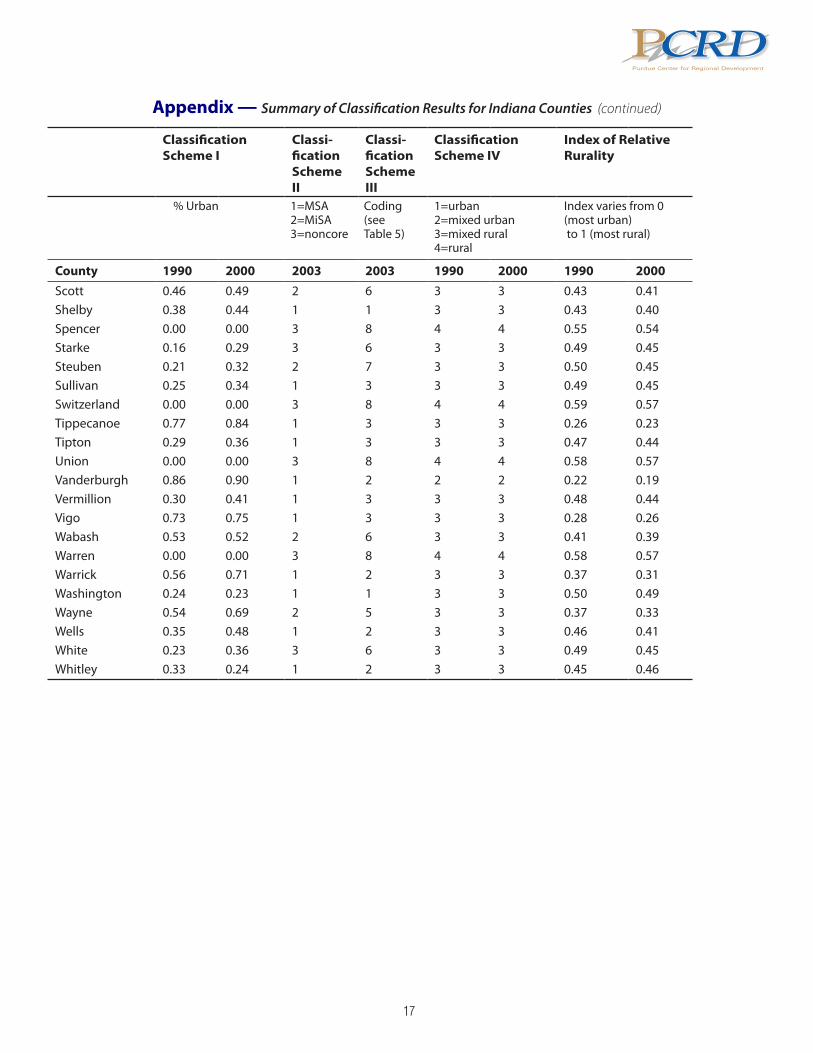
Appendix — Summary of Classification Results for Indiana Counties (continued)







Coding(see Table 5)



County 1990 2000 2003 2003 1990 2000 1990 2000Jasper 0.20 0.39 1 1 3 3 0.51 0.45Jay 0.42 0.43 3 6 3 3 0.44 0.43Jefferson 0.52 0.54 2 6 3 3 0.42 0.40Jennings 0.22 0.41 2 6 3 3 0.48 0.42Johnson 0.75 0.83 1 1 3 2 0.30 0.26Knox 0.58 0.64 2 4 3 3 0.41 0.38Kosciusko 0.27 0.47 2 4 3 3 0.44 0.38Lagrange 0.00 0.09 3 6 4 4 0.53 0.49Lake 0.95 0.95 1 1 1 1 0.20 0.19La Porte 0.57 0.65 1 3 3 3 0.32 0.29Lawrence 0.43 0.44 2 4 3 3 0.41 0.40Madison 0.67 0.76 1 3 3 3 0.29 0.25Marion 1.00 0.99 1 1 1 1 0.13 0.12Marshall 0.31 0.37 2 6 3 3 0.44 0.41Martin 0.28 0.26 3 6 3 3 0.52 0.51Miami 0.46 0.51 2 6 3 3 0.41 0.38Monroe 0.69 0.77 1 3 3 3 0.29 0.25Montgomery 0.39 0.44 2 6 3 3 0.44 0.41Morgan 0.31 0.46 1 1 3 3 0.43 0.38Newton 0.00 0.03 1 1 4 4 0.57 0.55Noble 0.30 0.34 2 6 3 3 0.45 0.42Ohio 0.00 0.00 1 1 4 4 0.58 0.56Orange 0.19 0.33 3 6 3 3 0.53 0.48Owen 0.15 0.00 1 3 3 4 0.51 0.53Parke 0.18 0.18 3 6 3 3 0.52 0.51Perry 0.42 0.48 3 6 3 3 0.46 0.43Pike 0.00 0.20 3 6 4 3 0.57 0.51Porter 0.67 0.78 1 1 3 2 0.30 0.26Posey 0.28 0.30 1 2 3 3 0.46 0.44Pulaski 0.00 0.19 3 6 4 3 0.58 0.52Putnam 0.30 0.28 1 1 3 3 0.47 0.46Randolph 0.32 0.36 3 6 3 3 0.46 0.43Ripley 0.16 0.18 3 6 3 3 0.51 0.49Rush 0.31 0.40 3 6 3 3 0.49 0.46St. Joseph 0.87 0.92 1 2 2 1 0.21 0.18

1�


CRDPAppendix — Summary of Classification Results for Indiana Counties (continued)







Coding(see Table 5)



County 1990 2000 2003 2003 1990 2000 1990 2000Scott 0.46 0.49 2 6 3 3 0.43 0.41Shelby 0.38 0.44 1 1 3 3 0.43 0.40Spencer 0.00 0.00 3 8 4 4 0.55 0.54Starke 0.16 0.29 3 6 3 3 0.49 0.45Steuben 0.21 0.32 2 7 3 3 0.50 0.45Sullivan 0.25 0.34 1 3 3 3 0.49 0.45Switzerland 0.00 0.00 3 8 4 4 0.59 0.57Tippecanoe 0.77 0.84 1 3 3 3 0.26 0.23Tipton 0.29 0.36 1 3 3 3 0.47 0.44Union 0.00 0.00 3 8 4 4 0.58 0.57Vanderburgh 0.86 0.90 1 2 2 2 0.22 0.19Vermillion 0.30 0.41 1 3 3 3 0.48 0.44Vigo 0.73 0.75 1 3 3 3 0.28 0.26Wabash 0.53 0.52 2 6 3 3 0.41 0.39Warren 0.00 0.00 3 8 4 4 0.58 0.57Warrick 0.56 0.71 1 2 3 3 0.37 0.31Washington 0.24 0.23 1 1 3 3 0.50 0.49Wayne 0.54 0.69 2 5 3 3 0.37 0.33Wells 0.35 0.48 1 2 3 3 0.46 0.41White 0.23 0.36 3 6 3 3 0.49 0.45Whitley 0.33 0.24 1 2 3 3 0.45 0.46


1�

Notes

1�


CRDP


�0


CRDP

3/07

Regional Development for Local Success

It is the policy of Purdue University that all persons shall have equal opportunity and access to the

programs and facilities without regard to race, color, sex, religion, national origin, age, marital status, parental status, sexual orientation, or disability.

Purdue University is an Affirmative Action institution.

Learn more about the Purdue Center for Regional Development, and find online versions of this and forthcoming publications at: http://www.purdue.edu/pcrd/

Documents

PCRD-R-4 What Is Rural and What Is Urban in Indiana? · publication explains the commonly used rural/urban classifications and what ... What Is Rural and What Is Urban in Indiana?