Embed Size (px)
Citation preview

Jurgen A. Doornik and David F. Hendry
Empirical Econometric Modelling
PcGiveTM 14 Volume I
OxMetrics 7
Published by Timberlake Consultants Ltdwww.timberlake.co.uk
www.timberlake-consultancy.comwww.oxmetrics.net, www.doornik.com

Empirical Econometric Modelling – PcGiveTM 14: Volume ICopyright c©2013 Jurgen A Doornik and David F Hendry
First published by Timberlake Consultants in 1998
Revised in 1999, 2001, 2006, 2009, 2013
All rights reserved. No part of this work, which is copyrighted, may be reproduced
or used in any form or by any means – graphic, electronic, or mechanical, including
photocopy, record taping, or information storage and retrieval systems – without the
written consent of the Publisher, except in accordance with the provisions of the
Copyright Designs and Patents Act 1988.
Whilst the Publisher has taken all reasonable care in the preparation of this book, the
Publisher makes no representation, express or implied, with regard to the accuracy
of the information contained in this book and cannot accept any legal responsability
or liability for any errors or omissions from the book, or from the software, or the
consequences thereof.
British Library Cataloguing-in-Publication DataA catalogue record of this book is available from the British Library
Library of Congress Cataloguing-in-Publication DataA catalogue record of this book is available from the Library of Congress
Jurgen A Doornik and David F Hendry
p. cm. – (Empirical Econometric Modelling – PcGiveTM 14: Vol I)
ISBN ISBN 978-0-9571708-3-4
Published byTimberlake Consultants Ltd
Unit B3, Broomsleigh Business Park 842 Greenwich Lane
London SE26 5BN, UK Union, NJ 07083-7905, U.S.A.
http://www.timberlake.co.uk http://www.timberlake-consultancy.com
Trademark noticeAll Companies and products referred to in this book are either trademarks or regis-
tered trademarks of their associated Companies.

Contents
Front matter iii
Contents v
List of Figures xiii
List of Tables xv
Preface xvii
I PcGive Prologue 1
1 Introduction to PcGive 31.1 The PcGive system . . . . . . . . . . . . . . . . . . . . . . . . . 31.2 Single equation modelling . . . . . . . . . . . . . . . . . . . . . 41.3 The special features of PcGive . . . . . . . . . . . . . . . . . . . 51.4 Documentation conventions . . . . . . . . . . . . . . . . . . . . 91.5 Using PcGive documentation . . . . . . . . . . . . . . . . . . . . 101.6 Citation . . . . . . . . . . . . . . . . . . . . . . . . . . . . . . . 111.7 World Wide Web . . . . . . . . . . . . . . . . . . . . . . . . . . 111.8 Some data sets . . . . . . . . . . . . . . . . . . . . . . . . . . . 11
II PcGive Tutorials 13
2 Tutorial on Cross-section Regression 152.1 Starting the modelling procedure . . . . . . . . . . . . . . . . . . 152.2 Formulating a regression . . . . . . . . . . . . . . . . . . . . . . 172.3 Cross-section regression estimation . . . . . . . . . . . . . . . . 18
2.3.1 Simple regression output . . . . . . . . . . . . . . . . . 202.4 Regression graphics . . . . . . . . . . . . . . . . . . . . . . . . 232.5 Testing restrictions and omitted variables . . . . . . . . . . . . . 242.6 Multiple regression . . . . . . . . . . . . . . . . . . . . . . . . . 26
v
vi CONTENTS
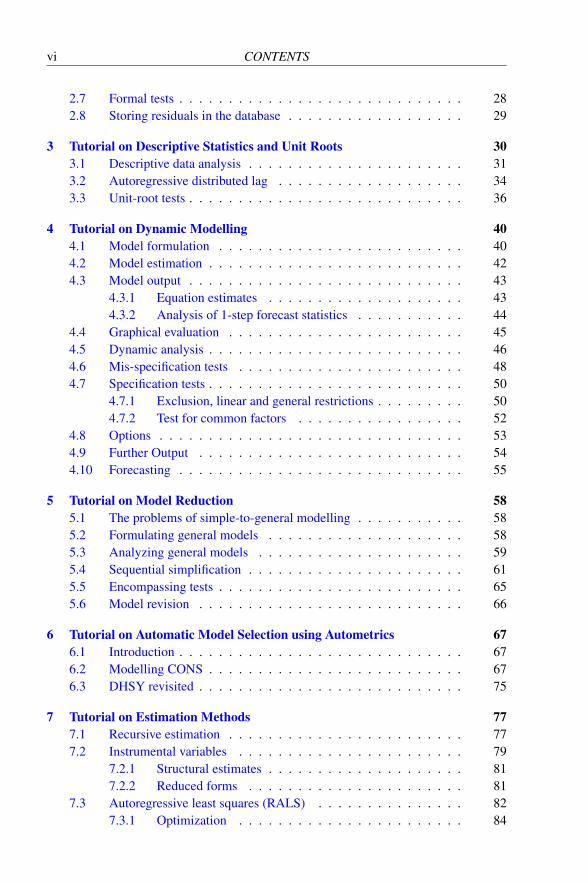
2.7 Formal tests . . . . . . . . . . . . . . . . . . . . . . . . . . . . . 282.8 Storing residuals in the database . . . . . . . . . . . . . . . . . . 29
3 Tutorial on Descriptive Statistics and Unit Roots 303.1 Descriptive data analysis . . . . . . . . . . . . . . . . . . . . . . 313.2 Autoregressive distributed lag . . . . . . . . . . . . . . . . . . . 343.3 Unit-root tests . . . . . . . . . . . . . . . . . . . . . . . . . . . . 36
4 Tutorial on Dynamic Modelling 404.1 Model formulation . . . . . . . . . . . . . . . . . . . . . . . . . 404.2 Model estimation . . . . . . . . . . . . . . . . . . . . . . . . . . 424.3 Model output . . . . . . . . . . . . . . . . . . . . . . . . . . . . 43
4.3.1 Equation estimates . . . . . . . . . . . . . . . . . . . . 434.3.2 Analysis of 1-step forecast statistics . . . . . . . . . . . 44
4.4 Graphical evaluation . . . . . . . . . . . . . . . . . . . . . . . . 454.5 Dynamic analysis . . . . . . . . . . . . . . . . . . . . . . . . . . 464.6 Mis-specification tests . . . . . . . . . . . . . . . . . . . . . . . 484.7 Specification tests . . . . . . . . . . . . . . . . . . . . . . . . . . 50
4.7.1 Exclusion, linear and general restrictions . . . . . . . . . 504.7.2 Test for common factors . . . . . . . . . . . . . . . . . 52
4.8 Options . . . . . . . . . . . . . . . . . . . . . . . . . . . . . . . 534.9 Further Output . . . . . . . . . . . . . . . . . . . . . . . . . . . 544.10 Forecasting . . . . . . . . . . . . . . . . . . . . . . . . . . . . . 55
5 Tutorial on Model Reduction 585.1 The problems of simple-to-general modelling . . . . . . . . . . . 585.2 Formulating general models . . . . . . . . . . . . . . . . . . . . 585.3 Analyzing general models . . . . . . . . . . . . . . . . . . . . . 595.4 Sequential simplification . . . . . . . . . . . . . . . . . . . . . . 615.5 Encompassing tests . . . . . . . . . . . . . . . . . . . . . . . . . 655.6 Model revision . . . . . . . . . . . . . . . . . . . . . . . . . . . 66
6 Tutorial on Automatic Model Selection using Autometrics 676.1 Introduction . . . . . . . . . . . . . . . . . . . . . . . . . . . . . 676.2 Modelling CONS . . . . . . . . . . . . . . . . . . . . . . . . . . 676.3 DHSY revisited . . . . . . . . . . . . . . . . . . . . . . . . . . . 75
7 Tutorial on Estimation Methods 777.1 Recursive estimation . . . . . . . . . . . . . . . . . . . . . . . . 777.2 Instrumental variables . . . . . . . . . . . . . . . . . . . . . . . 79
7.2.1 Structural estimates . . . . . . . . . . . . . . . . . . . . 817.2.2 Reduced forms . . . . . . . . . . . . . . . . . . . . . . 81
7.3 Autoregressive least squares (RALS) . . . . . . . . . . . . . . . 827.3.1 Optimization . . . . . . . . . . . . . . . . . . . . . . . 84

CONTENTS vii
7.3.2 RALS model evaluation . . . . . . . . . . . . . . . . . . 877.4 Non-linear least squares . . . . . . . . . . . . . . . . . . . . . . 88
8 Tutorial on Batch Usage 938.1 Introduction . . . . . . . . . . . . . . . . . . . . . . . . . . . . . 938.2 Generating and running Batch code . . . . . . . . . . . . . . . . 938.3 Generating and running Ox code . . . . . . . . . . . . . . . . . . 95
9 Non-linear Models 989.1 Introduction . . . . . . . . . . . . . . . . . . . . . . . . . . . . . 989.2 Non-linear modelling . . . . . . . . . . . . . . . . . . . . . . . . 989.3 Maximizing a function . . . . . . . . . . . . . . . . . . . . . . . 999.4 Logit and probit estimation . . . . . . . . . . . . . . . . . . . . . 1009.5 Tobit estimation . . . . . . . . . . . . . . . . . . . . . . . . . . . 1059.6 ARMA estimation . . . . . . . . . . . . . . . . . . . . . . . . . 1089.7 ARCH estimation . . . . . . . . . . . . . . . . . . . . . . . . . . 110
III The Econometrics of PcGive 113
10 An Overview 115
11 Learning Elementary Econometrics Using PcGive 11811.1 Introduction . . . . . . . . . . . . . . . . . . . . . . . . . . . . . 11811.2 Variation over time . . . . . . . . . . . . . . . . . . . . . . . . . 11911.3 Variation across a variable . . . . . . . . . . . . . . . . . . . . . 12011.4 Populations, samples and shapes of distributions . . . . . . . . . 12211.5 Correlation and scalar regression . . . . . . . . . . . . . . . . . . 12311.6 Interdependence . . . . . . . . . . . . . . . . . . . . . . . . . . 12611.7 Time dependence . . . . . . . . . . . . . . . . . . . . . . . . . . 12711.8 Dummy variables . . . . . . . . . . . . . . . . . . . . . . . . . . 12911.9 Sample variability . . . . . . . . . . . . . . . . . . . . . . . . . 13111.10 Collinearity . . . . . . . . . . . . . . . . . . . . . . . . . . . . . 13111.11 Nonsense regressions . . . . . . . . . . . . . . . . . . . . . . . . 133
12 Intermediate Econometrics 13512.1 Introduction . . . . . . . . . . . . . . . . . . . . . . . . . . . . . 13512.2 Linear dynamic equations . . . . . . . . . . . . . . . . . . . . . 136
12.2.1 Stationarity and non-stationarity . . . . . . . . . . . . . 13612.2.2 Lag polynomials . . . . . . . . . . . . . . . . . . . . . 136
12.2.2.1 Roots of lag polynomials . . . . . . . . . . . . 13812.2.2.2 Long-run solutions . . . . . . . . . . . . . . . 13812.2.2.3 Common factors . . . . . . . . . . . . . . . . 139
12.3 Cointegration . . . . . . . . . . . . . . . . . . . . . . . . . . . . 13912.4 A typology of simple dynamic models . . . . . . . . . . . . . . . 143

viii CONTENTS
12.4.1 Static regression . . . . . . . . . . . . . . . . . . . . . . 14512.4.2 Univariate autoregressive processes . . . . . . . . . . . 14512.4.3 Leading indicators . . . . . . . . . . . . . . . . . . . . 14612.4.4 Growth-rate models . . . . . . . . . . . . . . . . . . . . 14612.4.5 Distributed lags . . . . . . . . . . . . . . . . . . . . . . 14712.4.6 Partial adjustment . . . . . . . . . . . . . . . . . . . . . 14712.4.7 Autoregressive errors or COMFAC models . . . . . . . . 14812.4.8 Equilibrium-correction mechanisms . . . . . . . . . . . 14912.4.9 Dead-start models . . . . . . . . . . . . . . . . . . . . . 151
12.5 Interpreting linear models . . . . . . . . . . . . . . . . . . . . . 15112.5.1 Interpretation 1: a regression equation . . . . . . . . . . 15112.5.2 Interpretation 2: a (linear) least-squares approximation . 15212.5.3 Interpretation 3: an autonomous contingent plan . . . . . 15212.5.4 Interpretation 4: derived from a behavioural relationship 152
12.6 Multiple regression . . . . . . . . . . . . . . . . . . . . . . . . . 15312.6.1 Estimating partial adjustment . . . . . . . . . . . . . . . 15412.6.2 Heteroscedastic-consistent standard errors . . . . . . . . 15512.6.3 Specific-to-general . . . . . . . . . . . . . . . . . . . . 15612.6.4 General-to-specific (Gets) . . . . . . . . . . . . . . . . . 15912.6.5 Automatic model selection using Autometrics . . . . . . 16012.6.6 Time series . . . . . . . . . . . . . . . . . . . . . . . . 16212.6.7 Equilibrium correction . . . . . . . . . . . . . . . . . . 16212.6.8 Non-linear least squares, COMFAC, and RALS . . . . . 163
12.7 Econometrics concepts . . . . . . . . . . . . . . . . . . . . . . . 16612.7.1 Innovations and white noise . . . . . . . . . . . . . . . 16612.7.2 Exogeneity . . . . . . . . . . . . . . . . . . . . . . . . 16712.7.3 Constancy and invariance . . . . . . . . . . . . . . . . . 16812.7.4 Congruent models . . . . . . . . . . . . . . . . . . . . . 17012.7.5 Encompassing rival models . . . . . . . . . . . . . . . . 170
12.8 Instrumental variables . . . . . . . . . . . . . . . . . . . . . . . 17212.9 Inference and diagnostic testing . . . . . . . . . . . . . . . . . . 17312.10 Model selection . . . . . . . . . . . . . . . . . . . . . . . . . . . 175
12.10.1 Three levels of knowledge . . . . . . . . . . . . . . . . 17512.10.2 Modelling criteria . . . . . . . . . . . . . . . . . . . . . 17612.10.3 Implicit model design . . . . . . . . . . . . . . . . . . . 17612.10.4 Explicit model design . . . . . . . . . . . . . . . . . . . 177
13 Statistical Theory 17913.1 Introduction . . . . . . . . . . . . . . . . . . . . . . . . . . . . . 17913.2 Normal distribution . . . . . . . . . . . . . . . . . . . . . . . . . 17913.3 The bivariate normal density . . . . . . . . . . . . . . . . . . . . 180
13.3.1 Marginal and conditional normal distributions . . . . . . 18013.3.2 Regression . . . . . . . . . . . . . . . . . . . . . . . . . 181
13.4 Multivariate normal . . . . . . . . . . . . . . . . . . . . . . . . . 182

CONTENTS ix
13.4.1 Multivariate normal density . . . . . . . . . . . . . . . . 18213.4.2 Multiple regression . . . . . . . . . . . . . . . . . . . . 18313.4.3 Functions of normal variables: χ2, t and F distributions . 184
13.5 Likelihood . . . . . . . . . . . . . . . . . . . . . . . . . . . . . 18513.6 Estimation . . . . . . . . . . . . . . . . . . . . . . . . . . . . . 186
13.6.1 The score and the Hessian . . . . . . . . . . . . . . . . 18613.6.2 Maximum likelihood estimation . . . . . . . . . . . . . 18713.6.3 Efficiency and Fisher’s information . . . . . . . . . . . . 18813.6.4 Cramer–Rao bound . . . . . . . . . . . . . . . . . . . . 18913.6.5 Properties of Fisher’s information . . . . . . . . . . . . 18913.6.6 Estimating Fisher’s information . . . . . . . . . . . . . 190
13.7 Multiple regression . . . . . . . . . . . . . . . . . . . . . . . . . 19013.7.1 The multiple regression model . . . . . . . . . . . . . . 19113.7.2 Ordinary least squares . . . . . . . . . . . . . . . . . . . 19113.7.3 Distributional results . . . . . . . . . . . . . . . . . . . 19313.7.4 Subsets of parameters . . . . . . . . . . . . . . . . . . . 19413.7.5 Partitioned inversion . . . . . . . . . . . . . . . . . . . 19613.7.6 Multiple correlation . . . . . . . . . . . . . . . . . . . . 19713.7.7 Partial correlation . . . . . . . . . . . . . . . . . . . . . 19813.7.8 Maximum likelihood estimation . . . . . . . . . . . . . 19913.7.9 Recursive estimation . . . . . . . . . . . . . . . . . . . 199
14 Advanced Econometrics 20114.1 Introduction . . . . . . . . . . . . . . . . . . . . . . . . . . . . . 20114.2 Dynamic systems . . . . . . . . . . . . . . . . . . . . . . . . . . 20114.3 Data density factorizations . . . . . . . . . . . . . . . . . . . . . 204
14.3.1 Innovations and white noise . . . . . . . . . . . . . . . 20414.3.2 Weak exogeneity . . . . . . . . . . . . . . . . . . . . . 205
14.4 Model estimation . . . . . . . . . . . . . . . . . . . . . . . . . . 20614.5 Model evaluation . . . . . . . . . . . . . . . . . . . . . . . . . . 20714.6 Test types . . . . . . . . . . . . . . . . . . . . . . . . . . . . . . 20914.7 An information taxonomy . . . . . . . . . . . . . . . . . . . . . 210
14.7.1 The relative past . . . . . . . . . . . . . . . . . . . . . . 21014.7.2 The relative present . . . . . . . . . . . . . . . . . . . . 21114.7.3 The relative future . . . . . . . . . . . . . . . . . . . . . 21114.7.4 Theory information . . . . . . . . . . . . . . . . . . . . 21214.7.5 Measurement information . . . . . . . . . . . . . . . . . 21214.7.6 Rival models . . . . . . . . . . . . . . . . . . . . . . . 21314.7.7 The theory of reduction . . . . . . . . . . . . . . . . . . 214
14.8 Automatic model selection . . . . . . . . . . . . . . . . . . . . . 21514.8.1 Introduction . . . . . . . . . . . . . . . . . . . . . . . . 21514.8.2 Modelling strategies . . . . . . . . . . . . . . . . . . . . 21614.8.3 Models and the local DGP . . . . . . . . . . . . . . . . 21614.8.4 Costs of inference and costs of search . . . . . . . . . . 218
x CONTENTS
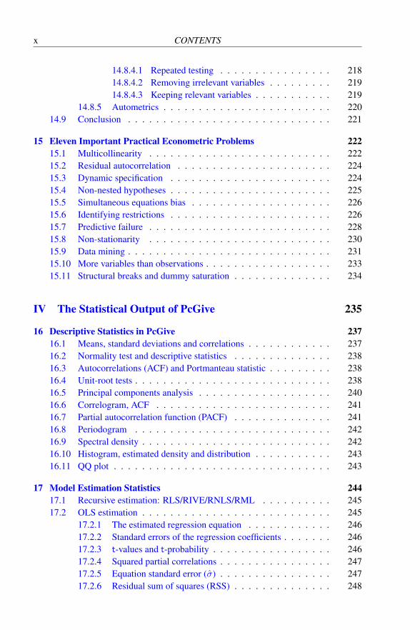
14.8.4.1 Repeated testing . . . . . . . . . . . . . . . . 21814.8.4.2 Removing irrelevant variables . . . . . . . . . 21914.8.4.3 Keeping relevant variables . . . . . . . . . . . 219
14.8.5 Autometrics . . . . . . . . . . . . . . . . . . . . . . . . 22014.9 Conclusion . . . . . . . . . . . . . . . . . . . . . . . . . . . . . 221
15 Eleven Important Practical Econometric Problems 22215.1 Multicollinearity . . . . . . . . . . . . . . . . . . . . . . . . . . 22215.2 Residual autocorrelation . . . . . . . . . . . . . . . . . . . . . . 22415.3 Dynamic specification . . . . . . . . . . . . . . . . . . . . . . . 22415.4 Non-nested hypotheses . . . . . . . . . . . . . . . . . . . . . . . 22515.5 Simultaneous equations bias . . . . . . . . . . . . . . . . . . . . 22615.6 Identifying restrictions . . . . . . . . . . . . . . . . . . . . . . . 22615.7 Predictive failure . . . . . . . . . . . . . . . . . . . . . . . . . . 22815.8 Non-stationarity . . . . . . . . . . . . . . . . . . . . . . . . . . 23015.9 Data mining . . . . . . . . . . . . . . . . . . . . . . . . . . . . . 23115.10 More variables than observations . . . . . . . . . . . . . . . . . . 23315.11 Structural breaks and dummy saturation . . . . . . . . . . . . . . 234
IV The Statistical Output of PcGive 235
16 Descriptive Statistics in PcGive 23716.1 Means, standard deviations and correlations . . . . . . . . . . . . 23716.2 Normality test and descriptive statistics . . . . . . . . . . . . . . 23816.3 Autocorrelations (ACF) and Portmanteau statistic . . . . . . . . . 23816.4 Unit-root tests . . . . . . . . . . . . . . . . . . . . . . . . . . . . 23816.5 Principal components analysis . . . . . . . . . . . . . . . . . . . 24016.6 Correlogram, ACF . . . . . . . . . . . . . . . . . . . . . . . . . 24116.7 Partial autocorrelation function (PACF) . . . . . . . . . . . . . . 24116.8 Periodogram . . . . . . . . . . . . . . . . . . . . . . . . . . . . 24216.9 Spectral density . . . . . . . . . . . . . . . . . . . . . . . . . . . 24216.10 Histogram, estimated density and distribution . . . . . . . . . . . 24316.11 QQ plot . . . . . . . . . . . . . . . . . . . . . . . . . . . . . . . 243
17 Model Estimation Statistics 24417.1 Recursive estimation: RLS/RIVE/RNLS/RML . . . . . . . . . . 24517.2 OLS estimation . . . . . . . . . . . . . . . . . . . . . . . . . . . 245
17.2.1 The estimated regression equation . . . . . . . . . . . . 24617.2.2 Standard errors of the regression coefficients . . . . . . . 24617.2.3 t-values and t-probability . . . . . . . . . . . . . . . . . 24617.2.4 Squared partial correlations . . . . . . . . . . . . . . . . 24717.2.5 Equation standard error (σ) . . . . . . . . . . . . . . . . 24717.2.6 Residual sum of squares (RSS) . . . . . . . . . . . . . . 248

CONTENTS xi
17.2.7 R2: squared multiple correlation coefficient . . . . . . . 24817.2.8 F-statistic . . . . . . . . . . . . . . . . . . . . . . . . . 24817.2.9 R2: Adjusted R2 . . . . . . . . . . . . . . . . . . . . . . 24917.2.10 Log-likelihood . . . . . . . . . . . . . . . . . . . . . . 24917.2.11 Mean and standard error of dependent variable . . . . . . 24917.2.12 *Information criteria . . . . . . . . . . . . . . . . . . . 25017.2.13 *Heteroscedastic-consistent standard errors (HCSEs) . . 25017.2.14 *R2 relative to difference and seasonals . . . . . . . . . 25017.2.15 *Correlation matrix of regressors . . . . . . . . . . . . . 25117.2.16 *Covariance matrix of estimated parameters . . . . . . . 25117.2.17 1-step (ex post) forecast analysis . . . . . . . . . . . . . 25117.2.18 Forecast test . . . . . . . . . . . . . . . . . . . . . . . . 25217.2.19 Chow test . . . . . . . . . . . . . . . . . . . . . . . . . 25317.2.20 t-test for zero forecast innovation mean (RLS only) . . . 253
17.3 IV estimation . . . . . . . . . . . . . . . . . . . . . . . . . . . . 25317.3.1 *Reduced form estimates . . . . . . . . . . . . . . . . . 25417.3.2 Structural estimates . . . . . . . . . . . . . . . . . . . . 25417.3.3 Specification χ2 . . . . . . . . . . . . . . . . . . . . . . 25517.3.4 Testing β = 0 . . . . . . . . . . . . . . . . . . . . . . . 25517.3.5 Forecast test . . . . . . . . . . . . . . . . . . . . . . . . 255
17.4 RALS estimation . . . . . . . . . . . . . . . . . . . . . . . . . . 25517.4.1 Initial values for RALS . . . . . . . . . . . . . . . . . . 25617.4.2 Final estimates . . . . . . . . . . . . . . . . . . . . . . 25717.4.3 Analysis of 1-step forecasts . . . . . . . . . . . . . . . . 25717.4.4 Forecast tests . . . . . . . . . . . . . . . . . . . . . . . 258
17.5 Non-linear modelling . . . . . . . . . . . . . . . . . . . . . . . . 25817.5.1 Non-linear least squares (NLS) estimation . . . . . . . . 25817.5.2 Maximum likelihood (ML) estimation . . . . . . . . . . 25917.5.3 Practical details . . . . . . . . . . . . . . . . . . . . . . 260
18 Model Evaluation Statistics 26318.1 Graphic analysis . . . . . . . . . . . . . . . . . . . . . . . . . . 26318.2 Recursive graphics (RLS/RIVE/RNLS/RML) . . . . . . . . . . . 26418.3 Dynamic analysis . . . . . . . . . . . . . . . . . . . . . . . . . . 266
18.3.1 Static long-run solution . . . . . . . . . . . . . . . . . . 26618.3.2 Analysis of lag structure . . . . . . . . . . . . . . . . . 267
18.3.2.1 Tests on the significance of each variable . . . 26718.3.2.2 Tests on the significance of each lag . . . . . . 268
18.3.3 Tests on the significance of all lags . . . . . . . . . . . . 26818.3.4 COMFAC tests . . . . . . . . . . . . . . . . . . . . . . 26818.3.5 Lag weights . . . . . . . . . . . . . . . . . . . . . . . . 268
18.4 Dynamic forecasting . . . . . . . . . . . . . . . . . . . . . . . . 26918.5 Diagnostic tests . . . . . . . . . . . . . . . . . . . . . . . . . . . 273
18.5.1 Introduction . . . . . . . . . . . . . . . . . . . . . . . . 273

xii CONTENTS
18.5.2 Residual autocorrelations (ACF), Portmanteau and DW . 27418.5.2.1 Durbin–Watson statistic (DW) . . . . . . . . . 275
18.5.3 Error autocorrelation test (not for RALS, ML) . . . . . . 27518.5.4 Normality test . . . . . . . . . . . . . . . . . . . . . . . 27618.5.5 Heteroscedasticity test using squares (not for ML) . . . . 27718.5.6 Heteroscedasticity test using squares and cross-products
(not for ML) . . . . . . . . . . . . . . . . . . . . . . . . 27718.5.7 ARCH test . . . . . . . . . . . . . . . . . . . . . . . . . 27718.5.8 RESET (OLS only) . . . . . . . . . . . . . . . . . . . . 27818.5.9 Parameter instability tests (OLS only) . . . . . . . . . . 27818.5.10 Diagnostic tests for NLS . . . . . . . . . . . . . . . . . 278
18.6 Linear restrictions test . . . . . . . . . . . . . . . . . . . . . . . 27818.7 General restrictions . . . . . . . . . . . . . . . . . . . . . . . . . 27918.8 Test for omitted variables (OLS) . . . . . . . . . . . . . . . . . . 27918.9 Progress: the sequential reduction sequence . . . . . . . . . . . . 27918.10 Encompassing and ‘non-nested’ hypotheses tests . . . . . . . . . 280
V Appendices 281
A1 Algebra and Batch for Single Equation Modelling 283A1.1 General restrictions . . . . . . . . . . . . . . . . . . . . . . . . . 283A1.2 Non-linear models . . . . . . . . . . . . . . . . . . . . . . . . . 284
A1.2.1 Non-linear least squares . . . . . . . . . . . . . . . . . . 284A1.2.2 Maximum likelihood . . . . . . . . . . . . . . . . . . . 284
A1.3 PcGive batch language . . . . . . . . . . . . . . . . . . . . . . . 285
A2 PcGive Artificial Data Set (data.in7/data.bn7) 292
A3 Numerical Changes From Previous Versions 294A3.1 From version 12 to 13 . . . . . . . . . . . . . . . . . . . . . . . 294A3.2 From version 9 to 10 . . . . . . . . . . . . . . . . . . . . . . . . 294A3.3 From version 8 to 9 . . . . . . . . . . . . . . . . . . . . . . . . . 295A3.4 From version 7 to 8 . . . . . . . . . . . . . . . . . . . . . . . . . 295
References 297
Author Index 309
Subject Index 311

Figures
2.1 Cross-plot of CONS against INC . . . . . . . . . . . . . . . . . . 202.2 Goodness-of-fit graphs for bivariate model of CONS . . . . . . . 242.3 Goodness-of-fit graphs for extended model of CONS . . . . . . . 27
3.1 Time-series plot of CONS and DCONS . . . . . . . . . . . . . . 303.2 Histogram and estimated density plot of CONS and DCONS . . . 343.3 Sample autocorrelation function of CONS and DCONS . . . . . . 34
4.1 Graphical evaluation of CONS model . . . . . . . . . . . . . . . 464.2 Lag weights from CONS model . . . . . . . . . . . . . . . . . . 484.3 Static and dynamic forecasts from CONS model . . . . . . . . . 56
5.1 Graphical statistics for the final model with 12 forecasts . . . . . 65
7.1 Recursive least squares graphical constancy statistics . . . . . . . 797.2 Autoregressive least squares grids . . . . . . . . . . . . . . . . . 867.3 Autoregressive least squares graphical statistics . . . . . . . . . . 877.4 Recursive non-linear least squares constancy statistics . . . . . . 92
9.1 Finney’s data . . . . . . . . . . . . . . . . . . . . . . . . . . . . 1019.2 Log-likelihoods, probabilities and outcomes for the logit model . 1039.3 Comparison of the probit and logit models . . . . . . . . . . . . . 1059.4 Comparison of fitted values from OLS and Tobit . . . . . . . . . 1079.5 Graphical analysis of ARMA(2,2) model . . . . . . . . . . . . . 1109.6 Graphical analysis for ARCH model using scaled actual and fitted 112
11.1 Time-series graphs of cons and inc . . . . . . . . . . . . . . . . . 11911.2 Histograms of cons and inc . . . . . . . . . . . . . . . . . . . . . 12011.3 Histograms and densities for cons and inc . . . . . . . . . . . . . 12111.4 QQ plots for cons and inc . . . . . . . . . . . . . . . . . . . . . 12211.5 Scatter plots for cons and inc . . . . . . . . . . . . . . . . . . . . 12311.6 Lagged scatter plots for cons and inc . . . . . . . . . . . . . . . . 12711.7 Sample ACF for cons and inc . . . . . . . . . . . . . . . . . . . 128
xiii

xiv LIST OF FIGURES
11.8 Relating time series and cross-plots using dummy variables . . . . 13011.9 Changing regression lines . . . . . . . . . . . . . . . . . . . . . 131
12.1 Goodness-of-fit measures for partial adjustment model . . . . . . 15712.2 Goodness-of-fit measures for ADL . . . . . . . . . . . . . . . . . 16112.3 Goodness-of-fit measures for EqCM . . . . . . . . . . . . . . . . 16412.4 Goodness-of-fit measures for RALS . . . . . . . . . . . . . . . . 16612.5 Mis-specified EqCM with near white-noise residuals . . . . . . . 16712.6 Recursive constancy statistics for EqCM . . . . . . . . . . . . . . 16912.7 Recursive constancy statistics for marginal, and invariance compari-
son . . . . . . . . . . . . . . . . . . . . . . . . . . . . . . . . . 17012.8 Recursive constancy statistics for IV estimation . . . . . . . . . . 174
14.1 From DGP to models . . . . . . . . . . . . . . . . . . . . . . . . 217

Tables
12.1 Model Typology . . . . . . . . . . . . . . . . . . . . . . . . . . 144
18.1 Empirical size of normality tests . . . . . . . . . . . . . . . . . . 276
A1.1 Batch language syntax summary . . . . . . . . . . . . . . . . . . 285
xv


Preface
PcGive for Windows is the latest in a long line of descendants of the original GIVEprogram. Over its life, many scholars, researchers and students have contributed to itspresent form. We are grateful to them all for their help and encouragement.
The current version, 14, has been designed to work with OxMetrics 7. This versionextends the automatic model selection to multivariate modelling. Version 13 offeredmore convenient access to the many econometric procedures in the program; version12 incorporated Autometrics for automatic model selection. It also introduced the auto-matic generation of Ox code in the background. PcGive remains almost entirely writtenin Ox. This complete rewrite for Ox was achieved with version 10.
The original mainframe ancestor was written in Fortran, PC versions in a mixtureof Fortran with some C and Assembly. Version 7 was a complete rewrite in C (with thegraphics in Assembly). Version 9 was a mixture of C and C++, while versions 10 andlater are written in Ox, with a small amount of code still in C.
Sections of code in PC-GIVE 6 were contributed by Neil Ericsson, Giuseppe Maz-zarino, Adrian Neale, Denis Sargan, Frank Srba and Juri Sylvestrowicz, and their im-portant contributions are gratefully acknowledged. Despite the algorithms having beenrewritten in C, their form and structure borrows from the original source. In particular,Adrian Neale’s code for graphics from PC-NAIVE was incorporated in PC-GIVE 6.0and much of that was carried forward to PcGive 7 and 8. The interface of PcGive 7 and8 was based on D-FLAT, developed by Al Stevens for Dr. Dobb’s Journal. Version 9relied on the Microsoft Foundation Class for its interface, for version 10 the interfaceis provided by OxPack. We are grateful to Bernard Silverman for permission to includehis code for density estimation.
Many people made the development of the program possible by giving their com-ments and testing out β-versions of version 10 and earlier versions. With the risk offorgetting some, we wish to thank Willem Adema, Peter Boswijk, Gunnar Bardsen,Mike Clements, Neil Ericsson, Bernd Hayo, Hans-Martin Krolzig, Bent Nielsen, Mar-ius Ooms, Jaime Marquez, and Neil Shephard for their help. We are also grateful tothe Oxford Institute of Economics and Statistics, especially to Gillian Coates, CandyWatts, and Alison Berry for help with earlier versions. We also wish to thank MaureenBaker and Nuffield College.
The documentation for GIVE has evolved dramatically over the years. We are in-debted to Mary Morgan and Frank Srba for their help in preparing the first (mainframe)
xvii

xviii PREFACE
version of a manual for GIVE. Our thanks also to Manuel Arellano, Giorgio Bodo, Pe-ter Boswijk, Julia Campos, Mike Clements, Neil Ericsson, Carlo Favero, Chris Gilbert,Andrew Harvey, Vivien Hendry, Søren Johansen, Siem Jan Koopman, Adrian Neale,Marius Ooms, Robert Parks, Jean-Francois Richard, Neil Shephard, Timo Terasvirtaand Giovanni Urga for their many helpful comments on the documentation for PC-GIVE 6 and later versions.
MikTeX in combination with Scientific Word and OxEdit eased the developmentof the documentation in LaTeX, further facilitated by the more self-contained nature ofrecent PcGive versions and the in-built help system.
Over the years, many users and generations of students have written with helpfulsuggestions for improving and extending PcGive, and while the current version willundoubtedly not yet satisfy all of their wishes, we remain grateful for their commentsand hope that they will continue to write with good ideas (and report any bugs!).
DFH owes a considerable debt to Evelyn and Vivien during the time he has spent onthis project: their support and encouragement were essential, even though they couldbenefit but indirectly from the end product. In a similar fashion, JAD is delighted tothank Kate for her support and encouragement.
We wish you enjoyable and productive use of
PcGive for Windows

Part I
PcGive Prologue


Chapter 1
Introduction to PcGive
1.1 The PcGive system
PcGive is an interactive menu-driven program for econometric modelling. PcGive ver-sion 14, to which this documentation refers, runs under Windows, Linux and OS X.PcGive originated from the AUTOREG Library (see Hendry and Srba, 1980, Hendry;Hendry, 1986b, 1993, Doornik and Hendry, 1992, and Doornik and Hendry, 1994), andis part of the OxMetrics family.
The econometric techniques of the PcGive system can be organized by the type ofdata to which they are (usually) applied. The documentation comprises three volumes,and the overview below gives in parenthesis whether the method is described in VolumeI, II or III. Volume IV refers to the PcNaive book.• Models for cross-section data
– Cross-section Regression (I)• Models for discrete data
– Binary Discrete Choice (III): Logit and Probit– Multinomial Discrete Choice (III): Multinomial Logit– Count data (III): Poisson and Negative Binomial
• Models for financial data– GARCH Models (III): GARCH in mean, GARCH with Student-t, EGARCH,
Estimation with Nelson&Cao restrictions• Models for panel data
– Static Panel Methods (III): within groups, between groups– Dynamic Panel Methods (III): Arellano-Bond GMM estimators
• Models for time-series data– Single-equation Dynamic Modelling (I), optionally using Autometrics– Multiple-equation Dynamic Modelling (II): VAR, cointegration, simultaneous
equations analysis– Regime Switching Models (III): Markov-switching– ARFIMA Models (III): exact maximum likelihood, modified-profile likelihood
3
4 Chapter 1 Introduction to PcGive
or non-linear least squares– Seasonal adjustment using X12Arima (III): regARIMA modelling, Automatic
model selection, Census X-11 seasonal adjustment.• Monte Carlo
– AR(1) Experiment using PcNaive (IV)– Static Experiment using PcNaive (IV)– Advanced Experiment using PcNaive & Ox Professional (IV)
• Other models– Nonlinear Modelling (I)– Descriptive Statistics (I):∗ Means, standard deviations and correlations∗ Normality tests and descriptive statistics∗ Autocorrelations (ACF) and Portmanteau statistic∗ Unit-root tests∗ Principal component analysis
PcGive uses OxMetrics for data input and graphical and text output. OxMetrics isdescribed in a separate book (Doornik and Hendry, 2013d). Even though PcGive islargely written in Ox (Doornik, 2013), it does not require Ox to function.
1.2 Single equation modellingThis book describes the single equation modelling features of PcGive. This part ofPcGive is designed for modelling economic data when the precise formulation of therelationship is not known a priori. The present version is for individual equations withjointly determined, weakly or strongly exogenous, predetermined, and lagged endoge-nous variables. A wide range of individual equation estimation methods is available.Particular features of the program are its ease of use, edit facilities, flexible data han-dling, extensive set of preprogrammed diagnostic tests, its focus on recursive methods,supported by powerful graphics, and the availability of automatic model selection. Sys-tem estimation methods are incorporated in PcGive, but described in a separate volume.
The documentation aims to provide an operational approach to econometric mod-elling using the most sophisticated yet easy-to-use software available. Thus, this book isespecially extensive to fully explain the econometric methods, the modelling approach,and the techniques used, as well as bridge the gap between econometric theory andempirical practice. It transcends the old ideas of ‘textbooks’ and ‘computer manuals’by linking the learning of econometric methods and concepts to the outcomes achievedwhen they are applied by the user at the computer. Because the program is so easyto learn and use, the main focus is on its econometrics and application to data anal-ysis. Detailed tutorials in Chapters 2–9 teach econometric modelling by walking theuser through the program in organized steps. This is supported by clear explanations ofeconometrics in Chapters 10–15. The material spans the level from introductory to fron-tier research, with an emphatic orientation to practical modelling. The exact definitionsof all statistics calculated by PcGive are described in Chapters 16–18. The context-

1.3 The special features of PcGive 5
sensitive help system supports this approach by offering help on both the program andthe econometrics.
This chapter discusses the special features of PcGive, describes how to use the doc-umentation, provides background information on data storage, interactive operation,help, results storage, and filenames, then outlines the basics of using the program (oftenjust point-and-click with a mouse).
1.3 The special features of PcGive
1. Ease of use• PcGive is user friendly, being a fully interactive and menu-driven approach
to econometric modelling: pull-down menus offer available options, and dialogboxes provide access to the available functions.
• PcGive has a high level of error protection, making it suitable for students ac-quiring experience in econometrics on computers, for live teaching in the class-room, or fraught late-night research.
• PcGive provides an extensive context-sensitive help system explaining both theprogram usage and the econometrics.
• High quality screen presentations in edit windows allow documentation ofresults as analysis proceeds, with easy review of previous results and cuttingand pasting within or between windows.
• Both text and graphics can be controlled by a mouse, allowing powerful andflexible editing, rapid menu and dialog access, and easy documentation ofgraphs.
• Estimation options can be set to automatically activate or inhibit model eval-uation procedures, set the format for results presentation and control the detailand sophistication of the output.
2. Advanced graphics• OxMetrics provides easy adjustment of graph types, layout and colours.• As many as 36 graphs can be shown simultaneously, with easy user control or
automatic selection.• Graphs can be documented and edited via direct screen access with reading
from the graph.• Time series and cross-plots are supported with flexible adjustment and scaling
options, including several bivariate linear regression lines with joint presentationof reverse regressions, or non-parametric fits, as well as spectra, correlograms,histograms and data densities.
• Descriptive results, recursive statistics, diagnostic tests, likelihood projec-tions and forecasts can be graphed in many combinations.
3. Flexible data handling in OxMetrics• The data handling system provides convenient storage of large data sets with
easy loading to PcGive either as a unit, or for subsamples or subsets of variables.

6 Chapter 1 Introduction to PcGive
• Excel and Lotus spreadsheet files can be loaded directly, or using ‘cut andpaste’ facilities.• Large data sets can be analyzed, with with as many variables and observations
as memory allows.• Database variables can be transformed by a calculator, or by entering mathe-
matical formulae in an editor with easy storage for reuse; the database is easilyviewed, incorrect observations are simple to revise, and variables can be docu-mented on-line.• Appending across data sets is simple, and the data used for estimation can be
any subset of the data in the database.• Several data sets can be open simultaneously, with easy switching between the
database.4. Efficient modelling sequence• The underlying Ox algorithms are fast, efficient, accurate and carefully
tested; all data are stored in double precision.• PcGive is designed specifically for modelling time-series data, and creates lags,
and analyzes dynamic responses and long-run relations with ease; it is simpleto change sample, or forecast, periods or estimation methods: models are re-tained for further analysis, and general-to-specific sequential simplifications aremonitored for reduction tests.• The structured modelling approach is fully discussed in this book, and guides
the ordering of menus and dialogs, but application of the program is completelyat the user’s control.• The estimators supported include least squares, instrumental variables, error
autocorrelation, non-linear least squares, and non-linear maximum likelihood:powerful numerical optimization algorithms are embedded in the program witheasy user control and most methods can be calculated recursively over the avail-able sample.• PcGive incorporates Autometrics for automatic model selection.• PcGive offers powerful preprogrammed testing facilities for a wide range
of hypotheses of interest to econometricians and economists undertaking sub-stantive empirical research, including tests for unit roots, dynamic specification,cointegration, linear restrictions and common factors.• PcGive is also applicable to cross-section data and most of its facilities and
tests are available for such analyses.• Large models can be formulated, with no restrictions on size, apart from those
imposed by available memory.• A Batch language allows automatic estimation and evaluation of models, and
can be used to prepare a PcGive session for teaching.5. Thorough evaluation• Equation mis-specification tests are automatically provided, including resid-
ual autocorrelation, autoregressive conditional heteroscedasticity (ARCH), het-eroscedasticity, functional form, parameter constancy, and normality (with

1.3 The special features of PcGive 7
residual density functions), as well as a complete set of encompassing tests.• The recursive estimators provide easy graphing of coefficients and residu-
als with their confidence intervals, or ‘t’-values: parameter constancy statisticsscaled by selected nominal significance levels are also calculated.
• All estimators provide graphs of fitted/actual values, residuals, and forecastsagainst outcomes with 1-step error bars.
6. Output• Graphs can be saved in several file formats including for later recall, further
editing, and printing, or for importing into many popular word processors, aswell as directly by ‘cut and paste’
• Results window information can be saved as an ASCII (human readable) doc-ument for input to most word processors, or directly input by ‘cut and paste’.
• Model residuals and recursive output can be stored in the database for addi-tional graphs or evaluation.
We now consider some of these special features in greater detail.
Advanced graphics• Users have full control over screen and graph colours. The colour, type (solid,
dotted, dashed etc.) and thickness of each line in a graph can be set; graphs can bedrawn inside boxes, and with or without grids; axis values can be automatic or userdefined; areas highlighted as desired; and so on.
• Up to 36 different graphs can be shown simultaneously on-screen, which is espe-cially valuable for graphical evaluation of equations and recursive methods. Com-binations of graphs displaying different attributes of data can be shown simultane-ously — examples are reported below.
• Once on-screen, text can be entered for graph documentation, or a mouse used tohighlight interesting features during live presentations. Graphs can be both rapidlysaved and instantly recalled. Coordinates can be read from each graph, howevermany are displayed at once.
• Much of PcGive’s output is provided in graphical form which is why it is writtenas an interactive (and not a batch) program. Dozens of time series can be graphedtogether using a wide range of adjustment and prescaling options. Two variablescan be cross-plotted as points or joined by lines (to show historical evolution), withleast-squares lines for subsamples, selected recursively (so growing in size) or se-quentially (a fixed % of the whole sample), showing projections of points from thelines; alternatively, both bivariate regression lines and/or a non-parametric regres-sion can be drawn. Or they can be plotted by the values of a third variable. Spectraldensities, correlograms, histograms and interpolated data densities and distributionsalso can be graphed in groups of up to 36.
• The option to see multiple graphs allows for more efficient evaluation of largeamounts of information. Blocks of graphs can simultaneously incorporate descrip-tive results (fitted and actual values, scaled residuals and forecasts etc.) and diag-nostic test information; or show many single-parameter likelihood grids.

8 Chapter 1 Introduction to PcGive
Efficient modelling sequence• Dynamic econometrics involves creating and naming lagged variables, controlling
the available sample and forecast period etc., and assigning the appropriate statusto all variables, so such operations are either automatic or very easy. The basic Pc-Give operator is a lag polynomial. Long-run solutions, unit-root tests, cointegrationtests, the significance of lagged variables (or groups of lags), the choice betweendeterministic or stochastic dynamics, roots of lag polynomials, tests for commonfactors etc. are all calculated. If the recommended general-to-specific approach tomodel construction is adopted, the sequence of reductions is monitored and F-tests,information criteria etc. are reported.
• This extensive program book seeks to bridge the gap between econometric theoryand empirical modelling: the tutorials walk the user through every step from in-putting data to the final selected econometric model of the variables under analysis.The econometrics chapters explain the theory and methods with reference to theprogram with detailed explanations of all the estimators and tests. The statisticaloutput chapters carefully define all the estimators and tests used by PcGive.
• The ordering of the menus and dialogs is determined by the theory: first estab-lish a data coherent, constant parameter model, investigate cointegration, reducethe model to a stationary, near orthogonal and simplified representation and finallycheck for parsimonious encompassing of the system: see Hendry and Ericsson(1991) and Hendry (1993), Hendry (1995a) for further details. Nevertheless, theapplication and sequence of the program’s facilities remain completely under theuser’s control.
• Estimation methods currently supported include ordinary and recursive leastsquares, two-stage least squares, instrumental variables and recursive instrumen-tal variables, rth-order autoregressive least squares, non-linear least squares andrecursive non-linear least squares and maximum likelihood. models are easily re-vised, transformed and simplified; up to 15 models are remembered for easy recalland progress evaluation.
• Powerful testing facilities for a wide range of specification hypotheses of interestto econometricians and economists undertaking substantive empirical research arepreprogrammed for automatic calculation. Available tests include dynamic specifi-cation, lag length, cointegration, and tests of reduction or parsimonious encompass-ing. Wald tests of linear restrictions are easily conducted.
• Automatic model selection is a recent advance in computational usage of econo-metrics. Starting from a general unrestricted model (denoted GUM), PcGive canimplement the model reduction for you–usually outperforming even expert econo-metricians. There are facilities for building models when there are more candidatevariables than observations.
Thorough evaluation• Evaluation tests can either be automatically calculated, calculated in a block as
a summary test option, or implemented singly or in sets merely by selecting therelevant dialog option. A comprehensive and powerful range of mis-specification

1.4 Documentation conventions 9
tests is offered to sustain the methodological recommendations about model evalua-tion. Equation mis-specification tests include residual autocorrelation, ARCH, het-eroscedasticity, functional form mis-specification and normality. Constancy testscan be computed automatically or via recursive procedures. A range of encompass-ing tests can be undertaken (just by a single keystroke or click!) once two rivalmodels have been estimated.
• Graphical diagnostic information includes plots of residual autocorrelation func-tions, residual density functions and histograms, and QQ plots.
• Much of the power of PcGive resides in its extensive use of recursive estimators.These provide voluminous output (coefficients, standard errors, t-values, residualsums of squares, 1-step residuals and their standard errors, constancy tests etc. atevery sample size), but recursive statistics can be graphed for easy presentation (upto 36 graphs simultaneously). The size of models is only restricted by the availablememory, as long as fewer than 100 variables are involved.
• All estimators provide graphs of residuals, fitted and actual values and their cross-plots, as well as 1-step forecasts or forecast errors with 95% confidence intervalsshown by error bars.
• Full graphics facilities can be applied to any or all of these graphs (e.g., addingregression lines etc.)
Considerable experience has demonstrated the practicality and value of using Pc-Give as an operational complement to learning econometrics and conducting empir-ical studies. It is also easy and helpful to run PcGive live in classroom teaching asan adjunct to theoretical derivations. On the research side, the incisive recursive esti-mators, the wide range of preprogrammed tests, and the powerful automatic selectionalgorithms make PcGive the most powerful interactive econometric modelling programavailable; Chapter 15 discusses its application to a range of important practical econo-metrics problems. These roles are enhanced by the flexible and informative graphicsoptions provided.
1.4 Documentation conventionsThe convention for instructions that you should type is that they are shown inTypewriter font. Capitals and lower case are only distinguished as the names ofvariables in the program and the mathematical formulae you type. Once OxMetricshas started, then from the keyboard, the Alt key accesses line menus (at the top of thescreen); from a mouse, click on the item to be selected using the left button. Commoncommands have a shortcut on the toolbar, the purpose of which can be ascertained byplacing the mouse on the relevant icon. Icons that can currently operate are highlighted.Commands on menus, toolbar buttons, and dialog items (buttons, checkboxes etc.) areshown in Sans Serif font.
Equations are numbered as (chapter.number); for example, (8.1) refers to equation8.1, which is the first equation in Chapter 8. References to sections have the form§chapter.section, for example, §8.1 is Section 8.1 in Chapter 8. Tables and Figures are
10 Chapter 1 Introduction to PcGive
shown as Figure chapter.number (e.g.) Figure 5.2 for the second figure in Chapter 5.Multiple graphs are numbered from left to right and top to bottom, so (b) is the top-rightgraph of four, and (c) the bottom left.
1.5 Using PcGive documentationThe documentation comes in five main parts: Part I comprises this introductory chapter,and instructions on starting the program. Part II then has six extensive tutorials on allaspects of econometric modelling, emphasizing the data analytic facilities over simplyprogram usage. Part III has six chapters discussing the econometrics of PcGive from in-troductory to advanced levels. Part IV offers a detailed description of the statistical andeconometric output of PcGive. Finally, Part V contains appendices. The documenta-tion ends with references and a subject index. As discussed above, the aim is to providea practical textbook of econometric modelling, linking the econometrics of PcGive toempirical modelling through tutorials which implement applied modelling exercises. Inmore detail:1. A separate book explains and documents the companion program OxMetrics which
records the output and provides data loading and graphing facilities.2. The Prologue discusses the main feature provided by PcGive, sketches how to use
the program and illustrates some of its output. In particular, Chapter 2 provides aquick start for the PcGive system.
3. The Tutorials in Chapters 2 to 9 are specifically designed for joint learning ofeconometric analysis and use of the programs. They describe using the editor, datainput, graphics control, dynamic model formulation, estimation and evaluation; dy-namic analysis; econometric modelling; and advanced features. By implementingempirical research exercises, they allow rapid mastery of PcGive and an understand-ing of how the associated econometric theory operates in practice.
4. The Econometric overview in Chapter 10 briefly reviews the background econo-metrics of PcGive.
5. Chapters 11–15 explain the Econometrics at all levels from elementary, throughintermediate to advanced, including Chapter 13 covering statistical theory, as wellas a chapter on important practical problems.
6. The Statistical Output in Chapters 16 to 18 explain in detail the econometric andstatistical calculations of PcGive.
7. Chapter A1 gives information about PcGive languages. The on-line help systemdocuments the menu structure and dialogs. Most dialogs are easy to understand, butthe on-line help can be accessed at any time if required.The appropriate sequence is to first install PcGive on your system. Next, read the
remainder of this introduction, then follow the step-by-step guidance given in the tuto-rials to get familiar with the operation of PcGive. Part III explains the required econo-metrics, starting at an elementary level and building up to advanced tools.
To use the documentation, either check the index for the subject, topic, menu or di-alog that seems relevant; or look up the part relevant to your current activity (for exam-

1.6 Citation 11
ple, econometrics, tutorials or description) in the Contents, and scan for the most likelykeyword. The references point to relevant publications which analyze the methodologyand methods embodied in PcGive.
1.6 CitationTo facilitate replication and validation of empirical findings, PcGive should be cited inall reports and publications involving its application. The appropriate form is to citePcGive in the list of references.
1.7 World Wide WebConsult www.doornik.com or www.oxmetrics.net pointers to additional informa-tion relevant to the current and future versions of PcGive. Upgrades are made availablefor downloading if required, and a demonstration version is also made available.
1.8 Some data setsThe data used in Hendry (1995a) is provided in the files ukm1.in7/ukm1.bn7. TheDHSY data (see Davidson, Hendry, Srba, and Yeo, 1978) is supplied in the filesdhsy.in7/dhsy.bn7. An algebra file, dhsy.alg, contains code to create variablesused in the paper. A batch file, dhsy.fl, loads the data, executes algebra code, andestimates the two final equations reported in the paper.
For the data sets used in Hendry and Morgan (1995), consult:www.nuff.ox.ac.uk/users/hendry.
Data sets accompanying Hendry and Nielsen (2007) can be found atwww.nuff.ox.ac.uk/users/nielsen/EconometricModeling.


Part II
PcGive Tutorials

Chapter 2
Tutorial on Cross-section Regression
2.1 Starting the modelling procedure
The purpose of this tutorial is to explain the use of PcGive for estimating linear regres-sion equations. The background to regression and least squares estimation methods isexplained in Chapters 11 and 12. If you are unfamiliar with regression, proceed withthis chapter till you feel lost, then read Chapter 11 and return here later. Our startingpoint is cross-section regression, because that has fewer options than dynamic regres-sion, making it easier to use.
Start OxMetrics, and load the data.in7 and data.bn7 files in OxMetrics as ex-plained in the OxMetrics book. If you have used this data set in a previous session, youcan right-click on the Data folder in the workspace, and look under Open Recent Data
File in the context menu. We assume that you’ve made yourself somewhat familiar withOxMetrics first, for example by reading the getting started chapters in the OxMetricsbook.
You can start modelling with PcGive from OxMetrics in three ways:• By clicking on the Model entry under Modules in the workspace on the left-hand
side.• Via Model on the Model menu.• Using the Model toolbar button:
Once started, the databases loaded in OxMetrics are accessible from PcGive.The modelling dialog gives access to all the modelling features of the OxMetrics
modules, including PcGive:
15
16 Chapter 2 Tutorial on Cross-section Regression
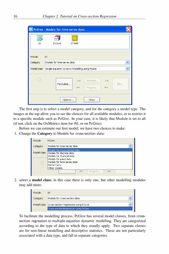
The first step is to select a model category, and for the category a model type. Theimages at the top allow you to see the choices for all available modules, or to restrict itto a specific module such as PcGive. In your case, it is likely that Module is set to all(if not, click on the OxMetrics item for All, or on PcGive).
Before we can estimate our first model, we have two choices to make:1. Change the Category to Models for cross-section data:
2. select a model class; in this case there is only one, but other modelling modulesmay add more:
To facilitate the modelling process, PcGive has several model classes, from cross-
section regression to multiple-equation dynamic modelling. They are categorizedaccording to the type of data to which they usually apply. Two separate classesare for non-linear modelling and descriptive statistics. These are not particularlyassociated with a data type, and fall in separate categories.

2.2 Formulating a regression 17
2.2 Formulating a regression
Selecting the cross-section regression using PcGive class, and pressing the Formulate
button takes you to the Model Formulation dialog:
This is a dialog which you will use often, so, at the risk of boring you, we consider itin detail. At the bottom are the two familiar OK and Cancel buttons, while the remainderis grouped in three columns. On the right are the variables that can be added to themodel and the databases that are open in OxMetrics. In the middle are buttons formoving between the database and the selection (i.e. the model). For dynamic models,the lag length is also there. On the left is current selection, options to change status, andthe possibility to recall previous models.
The following actions can be taken in this dialog:• Mark a variable by clicking on it with the mouse. To select several variables, use
the Ctrl key with the mouse, to select a range, use Shift plus the mouse.• Press >> to add selected variables to the model.• Double click to add a database variable to the model.• Remove a model variable by pressing >> or double clicking.• Empty the entire model formulation by pressing Clear>>.• The box immediately below the database contains the so-called ‘special’ variables.
These are made available even when not present in the database, and are added tothe selection in the same way as database variables.

18 Chapter 2 Tutorial on Cross-section Regression
• Below that, still on the database side, is the option to change databases, if more thanone are open in OxMetrics. But the model only works on one database.• On the left-hand side, below the selection (the model formulation), is a drop-down
box to change the status of selected variables. It becomes active when a selectionvariable is selected. For the cross-section regression there are three types:Y the endogenous (dependent) variable, by default the first,Z regressor, the default for all other variables,A an additional instrument (for instrumental variables estimation, considered in
Ch. 7),S an optional variable to select observations by.To change status, select one or more variables, then a status type, and click on Set.It is also possible to change status by right-clicking on a variable.
• Finally, the last drop-down box below the selection allows the recall of a previouslyformulated model (none as yet).
Select CONS and INC, and add the marked variables to the model, as shown in thecapture below:
The marked variable that is highest in the database becomes the dependent variable,because it is the first to enter the model. A two-step procedure might be required tomake a lower variable into the dependent variable: first mark and add the dependentvariable, then add the remaining variables.
Note that a Constant is automatically added, but can be deleted if the scale of thevariables lets a regression through the origin have meaning. CONS is marked with a Yto show that it is an endogenous (here, the dependent) variable. The other variables donot have a status letter, and default to regressor (Z).
2.3 Cross-section regression estimation
Pressing the OK button in the Model Formulation dialog immediately jumps to theEstimation dialog.

2.3 Cross-section regression estimation 19
Other ways of activating the Estimation dialog from OxMetrics are the short-cut keyAlt+l, in which the l stands for least squares; however, the toolbar button (the second:the blocks put together) will be the most convenient way of activating the dialog.
This style of dialog is used througout PcGive. It presents a list of options: checkboxes, edit fields, radio buttons etc. To change a value, click on the item with the mouse.A check box and radio button changes immediately; for an edit field the value can bechanged in the edit box. From the keyboard use the arrow up and down buttons to movebetween items, and the space bar to change the value. Pressing the return key has thesame effect as clicking the OK button, unless the caret is in an edit field.
Under cross-section regression, the only available option is estimation by ordinaryleast squares (OLS) (unless the model has more than one endogenous variable — ad-ditional estimation methods are discussed in Chapter 7).
The dialog allows selection of the sample period: by default the full sample is usedafter deleting observations which have missing values (as we shall discuss later, thesample can also be selected by a variable).
Press the OK button (or Enter) to estimate the model.The equation we fitted is:
CONSi = a+ bINCi + ui
where a and b are selected to minimize the sum of squares of the ui. The resultingestimated values for a and b are written a and b.
20 Chapter 2 Tutorial on Cross-section Regression
2.3.1 Simple regression output
The regression results are written to the Results window. As you may already know, thiswindow does not reside in PcGive, but in OxMetrics. After estimation, focus switchesautomatically to the Results window in OxMetrics. The output is:
EQ( 1) Modelling CONS by OLS-CSThe dataset is: .\OxMetrics7\data\data.in7The estimation sample is: 1953(1) - 1992(3)
Coefficient Std.Error t-value t-prob Part.R^2Constant -181.270 30.03 -6.04 0.000 0.1884INC 1.18563 0.03367 35.2 0.000 0.8876
sigma 4.5537 RSS 3255.58444R^2 0.887596 F(1,157) = 1240 [0.000]**Adj.R^2 0.88688 log-likelihood -465.639no. of observations 159 no. of parameters 2mean(CONS) 875.94 se(CONS) 13.5393
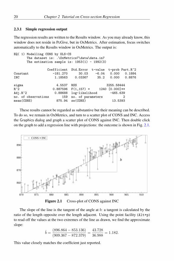
These results cannot be regarded as substantive but their meaning can be described.To do so, we remain in OxMetrics, and turn to a scatter plot of CONS and INC. Accessthe Graphics dialog and graph a scatter plot of CONS against INC. Then double clickon the graph to add a regression line with projections: the outcome is shown in Fig. 2.1.
CONS × INC
870 875 880 885 890 895 900 905 910
860
870
880
890
b
CONS × INC
Figure 2.1 Cross-plot of CONS against INC
The slope of the line is the tangent of the angle at b: a tangent is calculated by theratio of the length opposite over the length adjacent. Using the point facility (Alt+p)to read off the values at the two extremes of the line as drawn, we find the approximateslope:
b =(896.864− 853.136)
(909.367− 872.379)=
43.728
36.988= 1.182.
This value closely matches the coefficient just reported.

2.3 Cross-section regression estimation 21
The intercept is the value of CONS when INC equals zero, or more usefully, usingan overbar − to denote the mean value, a is given by:
a = CONS− b× INC.
To calculate the mean values, set focus to the data.in7 database in OxMetrics,and select Summary statistics from the View menu. The results from the descriptivestatistics are (we deleted the minimum and maximum):
Database: Data.in7Sample: 1953 (1) to 1992 (3) (159 observations)Variables: 4Variable leading sample #obs #miss mean std.devCONS 1953( 1)-1992( 3) 159 0 875.94 13.497INC 1953( 1)-1992( 3) 159 0 891.69 10.725INFLAT 1953( 1)-1992( 3) 159 0 1.7997 1.2862OUTPUT 1953( 1)-1992( 3) 159 0 1191.1 10.974
Substituting the means of the variables into our formula, we obtain:
a = 875.94− 1.182× 891.69 = −178.
Thus, the regression coefficients simply show the values of the slope and interceptneeded to draw the line in Figure 2.1. Their interpretation is that a unit increase in INCis associated with a 1.18 unit increase in CONS. If the data purport to be consumptionexpenditure and income, we should be suspicious of such a finding taken at face value.However, there is nothing mysterious about regression: it is simply a procedure forfitting straight lines to data. Once we have estimated the regression coefficients a andb, we can compute the fitted values:
CONSi = a+ b INCi,
and the residualsui = CONSi − CONSi.
The fitted values correspond to the straight line in Fig. 2.1, and the residuals to the ver-tical distance between the observed CONS values and the line (as drawn in the graph).
Next, the standard errors (SEs) of the coefficients reflect the best estimate of thevariability likely to occur in repeated random sampling from the same population: thecoefficient ±2SE provides a 95% confidence interval. When that interval does notinclude zero, the coefficient is often called ‘significant’ (at the 5% level). The number 2
derives from the assumption that β has a student-t distribution with n− k = 159− 2 =
157 degrees of freedom. This, in turn, we know to be quite close to a standard normaldistribution, and: P (|Z| > 2) ≈ 95% where Z ∼ N (0, 1).
The t-value of b is the ratio of the estimated coefficient to its standard error:
tb =b
SE(b) =
1.18563
0.03367= 35.2.

22 Chapter 2 Tutorial on Cross-section Regression
This can be used to test the hypothesis that b is zero (expressed as H0 : b = 0). Underthe current assumptions we reject the hypothesis if tb > 2 or tb < −2 (again, usinga 95% confidence interval, in other words, a 5% significance level), so values with|t| > 2 are significant. Here, the non-random residuals manifest in Figure 2.1 make theinterpretation of the SEs suspect (in fact, they are downwards biased here, and hencethe reported ‘t’-values are artificially inflated – despite that, they are so large that eventhe ‘correct’ SEs would yield t-values greater than 2 in absolute value).
The last statistic in the regression array is the partial r2. This is the squared correla-tion between the relevant explanatory variable and the dependent variable (often calledregressor and regressand respectively), holding all other variables fixed. For the regres-sion of CONS on INC, there are no other variables (after all, the Constant is not calledthat for nothing!), so the partial r2 equals the simple correlation squared (shown abovein the descriptive statistics output). As can be seen, that is also the value of the coeffi-cient of multiple correlation squared, R2, which measures the correlation between theactual values CONSi and the fitted values CONSi, and is reported immediately belowthe regression output. When there are several regressors, r2 and R2 differ.
Moving along the R2 row of output, the F-test is a test of R2 = 0. For a bivariateregression, that corresponds precisely to a test of b = 0 and can be checked usingthe fact that t2(k) = F(1, k). Here, (35.21)2 = 1239.74 which is close for a handcalculation. The next item [0.000] is the probability that F = 0, and the ∗∗ denotes thatthe outcome is significant at the 1% level or less.
The value of σ is the standard deviation of the residuals, usually called the equationstandard error:
σ =
√√√√ 1
n− k
n∑t=1
u2i ,
for n observations and k estimated parameters (regressors). Since the errors are as-sumed to be drawn independently from the same distribution with mean zero and con-stant variance σ, an approximate 95% confidence interval for any one error is 0 ± 2σ.That represents the likely interval from the fitted regression line of the observations.When σ = 4.55, the 95% interval is a huge 18.2% of CONS – the government wouldnot thank you for a model that poor, as it knows that consumers’ expenditure rarelychanges by more than 5% from one year to the next even without your model. We learnthat not all regressions are useful. RSS is the acronym from residual sum of squares,namely
∑nt=1 u
2i , which can be useful for hand calculations of tests between different
equations for the same variable.Finally, the last line gives the mean and variance of the dependent variable. The
variance corresponds to the squared standard deviation:1
CONS =1
n
n∑i=1
CONSi, [se(CONS)]2 = σ2y =
1
n− 1
n∑i=1
(CONSi − CONS
)2.
1Note that the column labelled std.dev in the summary statistics uses n in the denominatorgiving 13.497 for CONS. The regression output reports se(CONS)=13.5393, because it uses n−1.Also see §17.2.11.

2.4 Regression graphics 23
2.4 Regression graphics
Of course, there are other ways to represent the findings, and one of the more useful isa time-series graph of the fitted values, namely CONSi, with the outcomes, a cross-plotof the same two variables, and the scaled residuals:
ui =
(CONSi − CONSi
)σ
.
Select the Test menu in OxMetrics; again there are three ways Alt+t, Model/Test
or the Test toolbar button. Check Graphic analysis:
Press sf OK. The Graphic analysis dialog lets you plot and/or cross-plot the actualand fitted values, the residuals scaled by σ, the forecasts if any were assigned, and avariety of graphical diagnostics to which we return below. Mark Actual and fitted
values, Cross plot of actual and fitted, and Residuals (scaled) as shown here:
Accepting produces Figure 2.2 in OxMetrics. Any graphs can be saved, edited orprinted.

24 Chapter 2 Tutorial on Cross-section Regression
CONS Fitted
1955 1960 1965 1970 1975 1980 1985 1990
860
880
900CONS Fitted
CONS × Fitted
850 855 860 865 870 875 880 885 890 895 900
860
880
900CONS × Fitted
r:CONS (scaled)
1955 1960 1965 1970 1975 1980 1985 1990
-2
0
2
r:CONS (scaled)
Figure 2.2 Goodness-of-fit graphs for bivariate model of CONS
The first plot shows the ‘track’ of the outcome by the fitted model as time series.The overall tracking is fair, but is not very precise. This is perhaps easier to see herefrom the cross-plot, where two groups of scatters can be seen on either side of 875: theoutcome would be a straight line for a perfect fit. Finally, the scaled residuals do notlook very random: when the value is high in one period, you can see that it is morelikely to be high again in the next period, and similarly low (that is, large negative)values are followed by other low values.
2.5 Testing restrictions and omitted variablesWe will only compute two tests in this part of the tutorial: the first is for a subset of theregressors being zero. With only one actual variable, there is not much scope, but wecan check that the test yields the same outcome as the (squared) t-test already reported.Select the Test menu, Exclusion restrictions, and mark INC. Now accept to produce:
Test for excluding: INCSubset F(1,157) = 1239.8 [0.0000]**
This is identical to the F-test value above.The same test can be made through Test/Linear Restrictions. In this case restrictions
are entered in the formRβ = r,
where β is the k×1 coefficient vector, R the s×k restrictions matrix when s restrictionsare imposed, and r the desired value of the summation, an s × 1 vector. For a single

2.5 Testing restrictions and omitted variables 25
restriction in our simple model:
(R11 R12
)( a
b
)= r1.
Specifically, to test that b is zero:
(0 1
)( a
b
)= 0.
Access Test/Linear Restrictions and enter 0 1 0 in the edit field. The format is R
followed by r, so the leading 0 1 are the elements of R, and the final zero is r:
Further examples are given in the next chapter. Press OK to see:
Test for linear restrictions (Rb=r):R matrix
Constant INC0.00000 1.0000
r vector0.00000
LinRes F(1,157) = 1239.8 [0.0000]**
As a second test, we consider adding a variable to the existing model. SelectTest/Omitted variables and mark INFLAT as in:

26 Chapter 2 Tutorial on Cross-section Regression
This dialog offers a choice of lag length, provided that the lagged variables match theestimation sample (so no lags can be added here ). Accept to obtain:
Omitted variables test: F(1,156) = 149.072 [0.0000] **Added variables:[0] = INFLAT
This result strongly suggests that INFLAT has an important impact on the relationbetween CONS and INC, as the hypothesis that the effect is zero would essentiallynever produce such a large test outcome by chance.
2.6 Multiple regressionThat last result suggests using a multiple explanatory variable model, with both INCand INFLAT as regressors. From a methodological viewpoint, expanding a model inresponse to test rejections is not a good way to do research: we could have found 10different flaws with the first regression, and where we finally ended up would dependcritically on the order in which we ‘fixed’ them. However, in a tutorial on the use ofthe program, we can claim some poetic licence and proceed to the more interestingstage of a multiple regression by adding INFLAT to the set of regressors. Select Model,Formulate using the toolbar button, or the ‘hot-key’ Alt+y (remember yi is usually thesymbol for the dependent variable in econometrics since Koopmans, 1950).
Double click on INFLAT to add it to the model. Click on OK – then OK (or theEnter key) again at the Estimation dialog to obtain:

2.6 Multiple regression 27
EQ( 2) Modelling CONS by OLS-CSThe dataset is: .\OxMetrics7\data\data.in7The estimation sample is: 1953(1) - 1992(3)
Coefficient Std.Error t-value t-prob Part.R^2Constant -147.390 21.72 -6.79 0.000 0.2279INC 1.15263 0.02431 47.4 0.000 0.9351INFLAT -2.47468 0.2027 -12.2 0.000 0.4886
sigma 3.26673 RSS 1664.75821R^2 0.942522 F(2,156) = 1279 [0.000]**Adj.R^2 0.941785 log-likelihood -412.319no. of observations 159 no. of parameters 3mean(CONS) 875.94 se(CONS) 13.5393
Normality test: Chi^2(2) = 3.2519 [0.1967]Hetero test: F(4,154) = 0.26558 [0.8997]Hetero-X test: F(5,153) = 0.24667 [0.9409]RESET23 test: F(2,154) = 44.116 [0.0000]**
The added variable is apparently highly significant (but we shall see that we cannottrust in the standard errors reported).
The square of the t-test on INFLAT is precisely the Omitted variable F-test. Other-wise, the INC coefficient is not greatly altered, and still exceeds unity, but σ is some-what smaller, allowing a 95% confidence around the line of about 13% of CONS, whichremains too large for the model to be useful.
CONS Fitted
1960 1970 1980 1990
860
870
880
890
900 CONS Fitted
850 860 870 880 890 900
860
870
880
890
900
Fitted
CO
NS
rCONS (scaled)
1960 1970 1980 1990
-2
0
2rCONS (scaled) rCONS N(0,1)
-3 -2 -1 0 1 2 3
0.1
0.2
0.3
0.4
0.5 DensityrCONS N(0,1)
Figure 2.3 Goodness-of-fit graphs for extended model of CONS
The partial r2 for INC has risen relative to the simpler regression despite addingINFLAT: in fact INC only has a correlation of−0.11 with INFLAT. Nevertheless, some

28 Chapter 2 Tutorial on Cross-section Regression
of the explanation of CONS is being spread across the two regressor variables althoughmore is being explained in total. Replot the graphical output, this time marking theoptions for Actual and fitted values, Cross plot of actual and fitted, Residuals (scaled),and finally, Residual density and Histogram. The graphs now appear as in Figure 2.3.
The improvement in the fit over Figure 2.1 should be clear. The new plot is thehistogram with an interpolation of the underlying density. This lets us see the extent towhich the residuals are symmetric around zero, or have outliers etc.; more generally, itsuggests the form of the density. It is drawn together with the normal density (standard-ized, because the standardized residuals were used in the histogram and density).
2.7 Formal tests
Econometricians have constructed formal tests of such hypotheses as serial correlationor normality, and these are easily implemented in PcGive. A table of some of these testsis printed by default, starting with the normality test. To repeat this test for normality ofthe errors, select the Test... command from the Test menu and the Test dialog appears.Mark Normality as shown below, and accept.
The output comprises the first four moments of the residuals and a χ2 test for thesebeing from a normal distribution:
Normality test for ResidualsObservations 159Mean 0.00000Std.Devn. 3.2358Skewness -0.32415Excess Kurtosis -0.083166Minimum -9.0491Maximum 8.6025Asymptotic test: Chi^2(2) = 2.8303 [0.2429]Normality test: Chi^2(2) = 3.2519 [0.1967]
Note that the mean of the residuals is zero by construction when an intercept is in-cluded, and the standard deviation is the equation standard error (but uses the wrongdegrees of freedom, as it divides by n, rather than n− k). The skewness statistic mea-sures the deviation from symmetry, and the excess kurtosis measures how ‘fat’ the tailsof the distribution are: fat tails mean that outliers or extreme values are more common
2.8 Storing residuals in the database 29
than in a normal distribution. Finally, the largest and smallest values are reported. Here,the normality χ2 test does not reject: the probability of such a value or larger is 0.1967.
The data that are used here are time-series data, so we would really wish to includea test for the temperal assumptions as well. Further discussion of testing will appear inlater chapters.
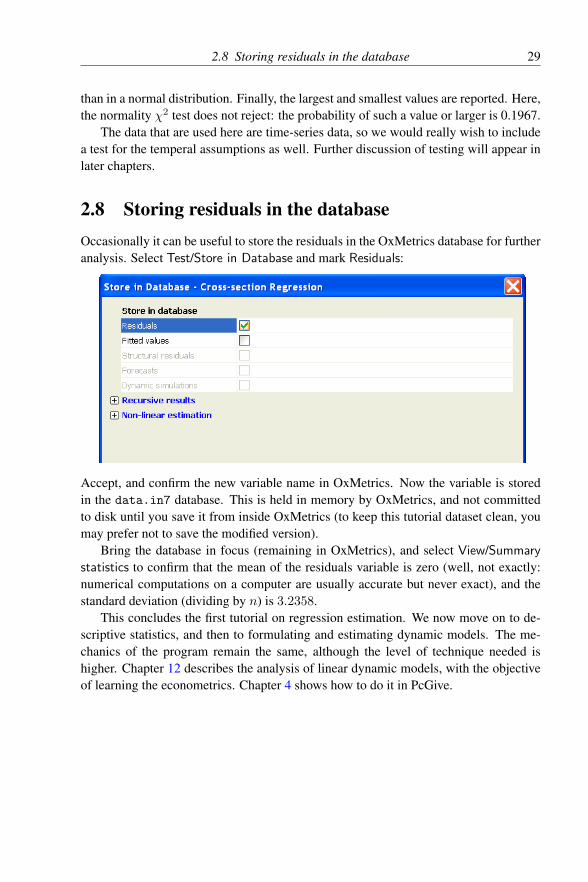
2.8 Storing residuals in the databaseOccasionally it can be useful to store the residuals in the OxMetrics database for furtheranalysis. Select Test/Store in Database and mark Residuals:
Accept, and confirm the new variable name in OxMetrics. Now the variable is storedin the data.in7 database. This is held in memory by OxMetrics, and not committedto disk until you save it from inside OxMetrics (to keep this tutorial dataset clean, youmay prefer not to save the modified version).
Bring the database in focus (remaining in OxMetrics), and select View/Summary
statistics to confirm that the mean of the residuals variable is zero (well, not exactly:numerical computations on a computer are usually accurate but never exact), and thestandard deviation (dividing by n) is 3.2358.
This concludes the first tutorial on regression estimation. We now move on to de-scriptive statistics, and then to formulating and estimating dynamic models. The me-chanics of the program remain the same, although the level of technique needed ishigher. Chapter 12 describes the analysis of linear dynamic models, with the objectiveof learning the econometrics. Chapter 4 shows how to do it in PcGive.

Chapter 3
Tutorial on Descriptive Statistics andUnit Roots
The previous tutorial introduced the econometrics of PcGive for a simple bivariate re-gression, and explained the mechanics of operating PcGive. We have mastered theskills to start the program, access menus and operate dialogs, load, save and transformdata, use graphics, including saving and printing and estimate simple regression mod-els. And remember, there is always help available if you get stuck: just press F1. Nowwe’re ready to move to more substantial activities. Usually, a data analysis starts by ex-ploring the data and transforming it to more interpretable forms. These activities are thesubject of this chapter. The OxMetrics book describes the ‘Calculator’ and ‘Algebra.’
If you’re not inside PcGive at the moment, restart and load the tutorial data setdata.in7/data.bn7 into OxMetrics.
Use the OxMetrics calculator to create DCONS as the first difference of CONS(in the calculator, mark CONS in the database list box, then press the Diff button andaccept lag length one to get the expression diff(CONS,1) in the calculator display,finally press the = button to accept DCONS). Fig. 3.1 shows how different CONS andDCONS appear when graphed.
CONS
1960 1970 1980 1990
860
870
880
890
CONS DCONS
1960 1970 1980 1990
-5.0
-2.5
0.0
2.5
5.0DCONS
Figure 3.1 Time-series plot of CONS and DCONS
30

3.1 Descriptive data analysis 31
3.1 Descriptive data analysis
In OxMetrics, select Model from the Model menu (or click on the Model toolbar icon).In the modelling dialog, select Other models as the category, and Descriptive Statistics
using PcGive for the model class:
Press the Formulate button to bring up the data selection dialog. This dialog is similarto that discussed in the previous section. Select CONS and DCONS:
In the next dialog, select means, standard deviations and correlations as shown here (theunit-root tests are described in §3.3):

32 Chapter 3 Tutorial on Descriptive Statistics and Unit Roots
Press OK, and OK again in the next dialog to accept the maximum sample size:
First listed in the output are the means and standard deviations, followed by thecorrelation matrix:
Means, standard deviations and correlations (using data.in7)The sample is: 1953(2) - 1992(3)Means
CONS DCONS875.85 -0.21341
Standard deviations (using T-1)CONS DCONS
13.533 2.2101Correlation matrix:
CONS DCONSCONS 1.0000 0.098638DCONS 0.098638 1.0000
The sample standard deviation of a variable x is defined here as
x =1
T
T∑t=1
xt, s =
√√√√ 1
T − 1
T∑t=1
(xt − x)2.
The sample correlation between two variables x and y is:
rxy =
∑Tt=1 (xt − x) (yt − y)√∑T
t=1 (xt − x)2∑T
t=1 (yt − y)2. (3.1)
CONS is hardly correlated with its difference, matching its high correlation with itsown one-lagged value (as we shall see later).

3.1 Descriptive data analysis 33
Now repeat, selecting Normality tests and descriptive statistics. The normality testoutput consists of the first four moments, extrema and a test statistic. The output is thesame as §2.7, but applied to CONS and DCONS instead of the model residuals:
Normality tests and descriptive statisticsThe dataset is: .\OxMetrics7\data\data.in7The sample is: 1953(2) - 1992(3)
Normality test for CONSObservations 158Mean 875.85Std.Devn. 13.490Skewness -0.17195Excess Kurtosis -1.6251Minimum 853.50Maximum 896.83Asymptotic test: Chi^2(2) = 18.165 [0.0001]**Normality test: Chi^2(2) = 52.808 [0.0000]**
Normality test for DCONSObservations 158Mean -0.21341Std.Devn. 2.2031Skewness -0.11208Excess Kurtosis -0.55302Minimum -5.4897Maximum 4.7393Asymptotic test: Chi^2(2) = 2.3442 [0.3097]Normality test: Chi^2(2) = 2.2958 [0.3173]
For a standard normal distribution (denoted by N(0, 1)) the numbers would be:
mean 0 skewness 0
standard deviation 1 excess kurtosis 0
Note the difference between the standard deviation of CONS under the normalitytest and under correlations. This can be explained by:
σ =
√√√√ 1
T
T∑t=1
(xt − x)2 versus s =
√√√√ 1
T − 1
T∑t=1
(xt − x)2.
The normality test reports the former:
13.490×√
158
157= 13.533.
The normality test statistic is a function of the skewness and excess kurtosis. Thevalue of the test for CONS is 52.81. The probability of getting a number at least as largeif CONS would really have a normal distribution is given between the square brackets.It is zero (not exactly, but so close to zero that we need not bother how close). Thetwo stars indicate that the test is significant at the 1% level, in other words it tells us

34 Chapter 3 Tutorial on Descriptive Statistics and Unit Roots
that 0% (the p-value) < 1%. It is extremely unlikely that CONS was generated by anormal distribution. DCONS is another picture, as we can see in Fig. 3.2: its shape isnot significantly different from an N(−0.21, (2.2)2) distribution.
CONS N(s=13.5)
850 860 870 880 890 900 910
0.02
0.04 CONS N(s=13.5) DCONS N(s=2.2)
-7.5 -5.0 -2.5 0.0 2.5 5.0 7.5
0.1
0.2DCONS N(s=2.2)
Figure 3.2 Histogram and estimated density plot of CONS and DCONS
3.2 Autoregressive distributed lag
ACF-CONS
0 5 10
0.5
1.0ACF-CONS ACF-DCONS
0 5 10
0
1ACF-DCONS
Figure 3.3 Sample autocorrelation function of CONS and DCONS
Figure 3.3 shows the sample autocorrelation function (ACF) of CONS and DCONS.CONS is highly correlated with its own lags, but not much autocorrelation is presentin DCONS, the distribution of which resembled an independent normal distribution inFig. 3.2b. Both graphs in Fig. 3.3 indicate approximate significance under the assump-tion that the data constitutes an independent sample from the normal distribution asabsolute values in excess of:
2
T 1/2=
2√159≈ 0.16
for the first graph (the second has T = 158, because one observation is lost when takingthe first difference).
From this, we could entertain the hypothesis that CONS is appropriately describedby a first-order autoregressive process, denoted by AR(1). In mathematical form:
yt = α+ βyt−1 + εt, t = 1, . . . , T. (3.2)

3.2 Autoregressive distributed lag 35
The coefficient α is the intercept. If β were zero, yt would be perturbed by a randomdisturbance around a constant. When β = 1, then ∆yt is random. Assumptions aboutthe error term are that it has mean 0 and variance which is constant over time:
E [εt] = 0, V [εt] = E [εt − E [εt]]2
= E[ε2t]
= σ2.
Autoregressions are a subset of autoregressive-distributed lag (ADL) models, andare easily estimated in PcGive using the techniques of the previous chapter. The onlydifference is that we need to estimate a dynamic model. Therefore, select the Models for
time-series data/Single-equation Dynamic Modelling menu to formulate a regressionof CONS on a Constant and CONS 1 (the first lag of CONS). The dialog is only slightlydifferent from before: a default lag length will be set (the initial default is one but canbe changed). After selecting one lag:
In the next screen, select ordinary least squares (the default), and then accept thedefault full sample period.
The estimation results from the AR(1) model are:
EQ( 3) Modelling CONS by OLSThe dataset is: .\OxMetrics7\data\data.in7The estimation sample is: 1953 (2) to 1992 (3)
Coefficient Std.Error t-value t-prob Part.R^2CONS_1 0.989378 0.01308 75.6 0.000 0.9734Constant 9.09221 11.46 0.793 0.429 0.0040

36 Chapter 3 Tutorial on Descriptive Statistics and Unit Roots
sigma 2.21251 RSS 763.648214R^2 0.97344 F(1,156) = 5717 [0.000]**Adj.R^2 0.973269 log-likelihood -348.658no. of observations 158 no. of parameters 2mean(CONS) 875.848 se(CONS) 13.5326
The output from simple regression was already discussed in §2.3.1. The col-umn marked coefficients gives β and α. Next to that are their estimated stan-dard errors, from which we could derive a rough 95% confidence interval, for β:(0.9894± 2× 0.01308). The number 2 derives from the assumption that β has astudent-t distribution with T − k = 158 − 2 = 156 degrees of freedom. This, in turn,we know to be quite close to a standard normal distribution. Soon we shall see that thisassumption might not be valid; if so, the confidence interval will change. Alternatively,we could use the t-value of β:
tβ =β
SE(β) =
0.9894
0.01308= 75.6
to test the hypothesis that β is zero (expressed as H0 : β = 0). Under the currentassumptions we reject the hypothesis if tβ > 2 or tβ < −2 (again, using a 95% confi-dence interval, in other words, a 5% significance level). The observed value of 75.6 isvery much larger than 2, making it highly unlikely that β is zero.
3.3 Unit-root testsIt is more interesting to test whether β equals one, H0 : β − 1 = 0. The t-value iscomputed as
0.9894− 1
0.01308= −0.8.
It is convenient to rewrite (3.2) by subtracting yt−1 from both sides:
yt − yt−1 = α+ βyt−1 − yt−1 + εt,
or:∆yt = α+ (β − 1) yt−1 + εt. (3.3)
With DCONS in the database, we can check whether (3.3) is identical to (3.2).Reformulate the model of the previous section as a regression of DCONS on a Constantand CONS 1. The result should be:EQ( 4) Modelling DCONS by OLS
The dataset is: .\OxMetrics7\data\data.in7The estimation sample is: 1953 (2) to 1992 (3)
Coefficient Std.Error t-value t-prob Part.R^2Constant 9.09221 11.46 0.793 0.429 0.0040CONS_1 -0.0106221 0.01308 -0.812 0.418 0.0042
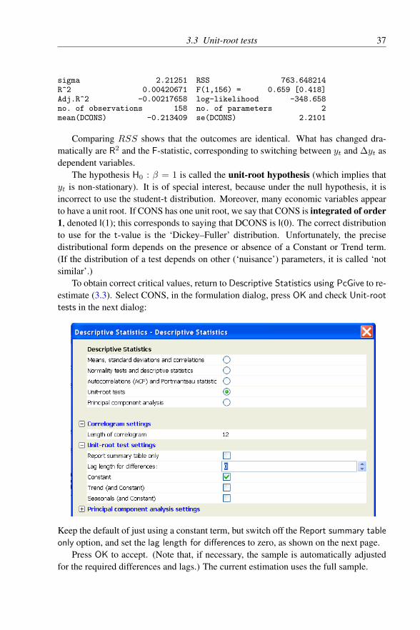
3.3 Unit-root tests 37
sigma 2.21251 RSS 763.648214R^2 0.00420671 F(1,156) = 0.659 [0.418]Adj.R^2 -0.00217658 log-likelihood -348.658no. of observations 158 no. of parameters 2mean(DCONS) -0.213409 se(DCONS) 2.2101
Comparing RSS shows that the outcomes are identical. What has changed dra-matically are R2 and the F-statistic, corresponding to switching between yt and ∆yt asdependent variables.
The hypothesis H0 : β = 1 is called the unit-root hypothesis (which implies thatyt is non-stationary). It is of special interest, because under the null hypothesis, it isincorrect to use the student-t distribution. Moreover, many economic variables appearto have a unit root. If CONS has one unit root, we say that CONS is integrated of order1, denoted I(1); this corresponds to saying that DCONS is I(0). The correct distributionto use for the t-value is the ‘Dickey–Fuller’ distribution. Unfortunately, the precisedistributional form depends on the presence or absence of a Constant or Trend term.(If the distribution of a test depends on other (‘nuisance’) parameters, it is called ‘notsimilar’.)
To obtain correct critical values, return to Descriptive Statistics using PcGive to re-estimate (3.3). Select CONS, in the formulation dialog, press OK and check Unit-root
tests in the next dialog:
Keep the default of just using a constant term, but switch off the Report summary table
only option, and set the lag length for differences to zero, as shown on the next page.Press OK to accept. (Note that, if necessary, the sample is automatically adjusted
for the required differences and lags.) The current estimation uses the full sample.

38 Chapter 3 Tutorial on Descriptive Statistics and Unit Roots
Unit-root testsThe dataset is: .\OxMetrics7\data\data.in7The sample is: 1953(2) - 1992(3)
Augmented Dickey-Fuller test for CONS; regression of DCONS on:Coefficient Std.Error t-value
CONS_1 -0.010622 0.013085 -0.81180Constant 9.0922 11.464 0.79309
sigma = 2.21251 DW = 1.598 DW-CONS = 0.02639 ADF-CONS = -0.8118Critical values used in ADF test: 5%=-2.88, 1%=-3.473RSS = 763.6482142 for 2 variables and 158 observations
DW is the Durbin-Watson statistic of the OLS regression residuals, whereas DW-CONS is the Durbin-Watson of CONS (see Chapter 16). ADF-CONS is the t-statisticwe computed earlier. The 5% critical value for the Dickey–Fuller test is reported as−2.88. The negative number is given, because the interesting alternative hypothesis isthat β < 1; β > 1 corresponds to an exploding process, which we tend not to see ineconomic variables. The critical values are based on response surfaces in MacKinnon(1991); 5% significance is marked by *, 1% by **. Here we can not reject the hypothesisthat β − 1 = 0: CONS appears to have a unit root (is I(1)). As with all statisticaltests, some caution is required. It can be seen in the time-series graph of CONS inFig. 3.1a that it has a break around 1975, and it has been found that a break can causeI(0) variables to appear I(1) in DF tests.
The augmented Dickey–Fuller (ADF) test derives from the DF test by adding laggeddifferences, for example, for the ADF(1) test:
∆yt = α+ (β − 1) yt−1 + γ∆yt−1 + εt,
or more generally for the ADF(s):
∆yt = α+ (β − 1) yt−1 +
s∑i=1
γi∆yt−i + εt.
ADF(0) corresponds to the DF test. The purpose of these additional lags is to ‘whiten’the residuals, reducing their autocorrelation.
Tip The null hypothesis is that of a unit root. A significant test statistic would rejectthat hypothesis and suggest stationarity.
To facilitate the computation of ADF tests, and the decision about the lag length, Pc-Give can be instructed to print a summary table of ADF tests. Select Model/Descriptive
Statistics, mark INFLAT and CONS, and select Unit-root tests. The default isthe summary table starting from lag 4. The output consists of the sequence ofADF(4). . . ADF(0) tests:

3.3 Unit-root tests 39
Unit-root tests (using data.in7)The sample is 1954 (2) - 1992 (3)
CONS: ADF tests (T=154, Constant; 5%=-2.88 1%=-3.47)D-lag t-adf beta Y_1 sigma t-DY_lag t-prob AIC F-prob4 -1.466 0.98058 2.157 1.268 0.2068 1.5763 -1.308 0.98278 2.161 1.450 0.1492 1.573 0.20682 -1.135 0.98512 2.169 1.712 0.0889 1.574 0.15941 -0.9463 0.98759 2.183 2.491 0.0138 1.581 0.08740 -0.6500 0.99139 2.220 1.608 0.0135
INFLAT: ADF tests (T=154, Constant; 5%=-2.88 1%=-3.47)D-lag t-adf beta Y_1 sigma t-DY_lag t-prob AIC F-prob4 -5.095** 0.85178 0.3534 0.5232 0.6016 -2.0423 -5.340** 0.85784 0.3526 1.078 0.2829 -2.053 0.60162 -5.354** 0.86932 0.3527 1.090 0.2774 -2.058 0.49101 -5.363** 0.87997 0.3530 11.40 0.0000 -2.063 0.45770 -2.398 0.92835 0.4799 -1.456 0.0000
The first column is the number of lagged differences, so the first line gives theresults for the ADF(4) test. The second column is the t-value, which is the ADF teststatistic, the third column is the coefficient on yt−1 (the coefficient used in t-adf), thenext column gives the equation standard error. The next two columns, t-DY lag andt-prob, give the t-value of the longest lag (of γs, s = 4, 3, 2, 1), followed by the p-valueof that lag. The suggested strategy is to select the highest swith a significant last γs (thedistribution of γs is the conventional student-t distribution). So for both INFLAT andCONS we use an ADF(1) test. The only place where it makes a difference is in usingADF(1) or ADF(0) for INFLAT. Using the lag criterion we conclude that INFLAT isstationary, so if we did not check for the importance of lagged values of INFLAT, wemight mistakenly think that it is non-stationary. Note that all tests used the same sampleperiod, which explains why the table lists ADF-CONS(0)= −0.65, while we previouslyfound −0.81. We deleted the column labelled AIC; the last column, labelled F-prob, isthe p-value of the F-tests on all lags dropped up to that point.
We have avoided the issue of including a constant, or a constant and trend. Theimplications are as follows:
β = 1 β < 1
∆yt = (β − 1) yt−1 + εt zero growth mean zero∆yt = α+ (β − 1) yt−1 + εt trend in yt non-zero mean∆yt = α+ (β − 1) yt−1 + µt+ εt quadratic trend in yt trend in yt
Few variables have quadratic trends, but it is often advisable to include t in case thevariable is stationary around a linear trend. Equally, include an intercept unless it isclear that the variable has a zero mean. Technically, including a polynomial in time oforder n (for example, having α and µt corresponds to n = 1) makes the test similardespite the presence of the nuisance parameters of a polynomial of order n− 1.
Some variables could be thought to be I(2). Then you could start with checkingwhether the second differences are I(0). If so, move on to the first differences.
That concludes the data description. The PcGive unit-root test and issues of cointe-gration are discussed in §12.6.

Chapter 4
Tutorial on Dynamic Modelling
Dynamic modelling normally consists of a cycle of three steps: formulation or re-formulation, estimation and evaluation. The modelling process takes place within theModel and the Test menus described in the previous tutorials, but we reproduce severaldialogs here for convenience. This tutorial will guide you through a simple model se-quence based on the artificial data set. Hopefully you will agree at the end that PcGivecombines sophistication with great simplicity.
Before we start, a brief digression on lags is called for. PcGive names lagged vari-ables by appending an underscore and then the lag length. So CONS 1 is CONS oneperiod lagged. PcGive uses this naming scheme to keep track of the lag length. Sup-pose the database holds both a CONS and a CONS 1 variable. Then, when formulatinga model involving the first lag of CONS, PcGive will use CONS, to create that lag. Sothe database CONS 1 variable is never used. When CONS 1 is the only CONS variablein the database, PcGive will start using it.
4.1 Model formulation
Load data.in7 in OxMetrics, if you are starting this tutorial afresh. Then click onthe Model icon (or use Model on the Model menu or Alt+y). Change the Category toModels for time series data and the Model class to Single-equation dynamic modelling
using PcGive:
40
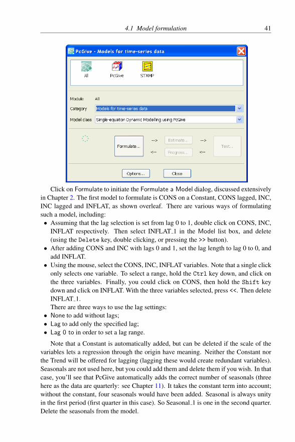
4.1 Model formulation 41
Click on Formulate to initiate the Formulate a Model dialog, discussed extensivelyin Chapter 2. The first model to formulate is CONS on a Constant, CONS lagged, INC,INC lagged and INFLAT, as shown overleaf. There are various ways of formulatingsuch a model, including:• Assuming that the lag selection is set from lag 0 to 1, double click on CONS, INC,
INFLAT respectively. Then select INFLAT 1 in the Model list box, and delete(using the Delete key, double clicking, or pressing the >> button).
• After adding CONS and INC with lags 0 and 1, set the lag length to lag 0 to 0, andadd INFLAT.
• Using the mouse, select the CONS, INC, INFLAT variables. Note that a single clickonly selects one variable. To select a range, hold the Ctrl key down, and click onthe three variables. Finally, you could click on CONS, then hold the Shift keydown and click on INFLAT. With the three variables selected, press <<. Then deleteINFLAT 1.There are three ways to use the lag settings:
• None to add without lags;• Lag to add only the specified lag;• Lag 0 to in order to set a lag range.
Note that a Constant is automatically added, but can be deleted if the scale of thevariables lets a regression through the origin have meaning. Neither the Constant northe Trend will be offered for lagging (lagging these would create redundant variables).Seasonals are not used here, but you could add them and delete them if you wish. In thatcase, you’ll see that PcGive automatically adds the correct number of seasonals (threehere as the data are quarterly: see Chapter 11). It takes the constant term into account;without the constant, four seasonals would have been added. Seasonal is always unityin the first period (first quarter in this case). So Seasonal 1 is one in the second quarter.Delete the seasonals from the model.

42 Chapter 4 Tutorial on Dynamic Modelling
4.2 Model estimation
Estimation methods are discussed in Chapter 12; Chapter 17 reviews the statistical out-put reported following estimation. Here we only need OLS; examples of the otherestimation methods are given in the next chapter. Pressing OK after model formulationbrings up the model settings dialog. Select the default of OLS:
The next step is the the Estimation dialog where the sample period can be set. Theshort-cut key for model estimation is Alt+l, in which the l stands for least squares.However, pressing OK in the Model Settings dialog takes us directly to the Estimation
dialog.

4.3 Model output 43
The dialog also allows you to retain some data for static forecasting. The sampleperiod can be adjusted, but the one shown is always admissible and will either be themaximum available or the one used in the previous model. Please verify that the samplesize on your screen corresponds to the one shown here, the full sample: 1953 (2) – 1992(3). Retain eight observations for parameter constancy using the Less forecasts textentry field (the default is none, and the maximum is determined by the sample size):
Tip It is easy to refit models to subsamples and hence conduct tests of constancy basedon the residual sums of squares. The recursive estimation option allows testing overthe entire set of subsamples.
4.3 Model output
4.3.1 Equation estimates
The estimated equation has the form:
yt = x′tβ + εt, t = 1, . . . , T,
where xt contains a ‘1’ for the intercept, yt−1 for the lagged dependent variable, aswell as the other regressors. Assumptions about the error term are that it has mean 0and variance which is constant over time:
E [εt] = 0, V [εt] = E [εt − E [εt]]2
= E[ε2t]
= σ2.
We can write the estimated autoregressive-distributed lag (ADL) model in more detailas:
CONSt = a1CONSt−1 + c+ b0INCt + b1INCt−1 + γINFLATt + εt. (4.1)
The equation estimation results are written to the OxMetrics Results window wherefurther editing is easy. We assume that you have the default options setting, whichgenerates the minimum number of statistics. Section 4.8 discusses the options. The re-ported results include coefficient estimates; standard errors; t-values; the squared partial

44 Chapter 4 Tutorial on Dynamic Modelling
correlation of every regressor with the dependent variable; the squared multiple corre-lation coefficient (denoted R2); an F-test on R2 equalling zero; the equation standarderror (σ); the Residual Sum of Squares (RSS); these were all introduced in §2.3.1.EQ( 1) Modelling CONS by OLS (using data.in7)
The estimation sample is: 1953(2) - 1990(3)
Coefficient Std.Error t-value t-prob Part.R^2CONS_1 0.809091 0.02548 31.8 0.000 0.8743Constant -18.5178 8.726 -2.12 0.036 0.0301INC 0.506687 0.02882 17.6 0.000 0.6807INC_1 -0.296493 0.03560 -8.33 0.000 0.3236INFLAT -0.992567 0.08618 -11.5 0.000 0.4777
sigma 1.07598 RSS 167.872396R^2 0.993693 F(4,145) = 5712 [0.000]**Adj.R^2 0.993519 log-likelihood -221.283no. of observations 150 no. of parameters 5
1-step (ex post) forecast analysis 1990(4) - 1992(3)Parameter constancy forecast tests:Forecast Chi^2(8) = 9.3241 [0.3157]Chow F(8,145) = 1.1500 [0.3337]
The sample period was automatically adjusted for the lags created on CONS andINC. The figure in [·] after the F (·) value is the probability of obtaining that value froma central F-distribution with the degrees of freedom shown. Should it be desired, theoutput can also be printed in LATEX or equation format, as shown in §4.8.
4.3.2 Analysis of 1-step forecast statistics
The forecast tests are a Chow test and a forecast Chi2 (8) which is an index of numericalparameter constancy. For H forecasts, values > 2H imply poor ex ante accuracy.The χ2 value always exceeds that of H times the Chow test. Later, we will graph theoutcomes, forecasts and the error bars for ±2 standard errors of the 1-step forecasts.The forecast tests are reported with the regression output. To see the full results, selectTest/Further Output, and select Static (1-step) forecasts:

4.4 Graphical evaluation 45
1-step forecasts for CONS (SE with parameter uncertainty)Horizon Forecast SE Actual Error t-value1990-4 862.235 1.097 861.484 -0.751532 -0.6851991-1 862.136 1.090 864.444 2.30801 2.1171991-2 863.237 1.085 862.750 -0.487490 -0.4491991-3 860.146 1.091 859.413 -0.732399 -0.6711991-4 862.243 1.106 860.480 -1.76260 -1.5941992-1 860.796 1.092 860.002 -0.793439 -0.7271992-2 856.477 1.113 855.908 -0.568310 -0.5111992-3 856.995 1.089 856.731 -0.264312 -0.243
mean(Error) = -0.38151 RMSE = 1.1616SD(Error) = 1.0972 MAPE = 0.11126
The RMSE and MAPE are discussed in §4.10.
4.4 Graphical evaluation
The next major step is to evaluate the estimated model. Select the Graphic Analysis
dialog from the Test menu (or press the toolbar button), and mark the first six items:
The dialog lets you plot or cross-plot the actual and fitted values for the wholesample, the residuals scaled by σ, so that values outside the range [−2,+2] suggestoutlier problems, the forecasts, and some graphical diagnostic information about theresiduals (their spectrum, correlogram, histogram, density and cumulative distribution).The forecast period start is marked by a vertical line (see Figure 4.1). Notice the goodfit: the earlier high R2, and good Chow test are consistent with this. As before, anygraphs can be saved for later recall, editing and printing.
Accept the dialog, and the graphs appear in the PcGive Graphics window in Ox-Metrics, as in Figure 4.1. There are two new graphs. The first is the correlogram, whichextends the idea behind the DW test to plot the correlations between successive laggedresiduals (that is, the correlation of εt with εt−1, then with εt−2, εt−3 and so on up toεt−12). A random (independent) residual would have most such correlations close tozero: visually, the dependence between successive residuals is small. The second plotsthe forecasts which we printed earlier, with the error bands changed to error fans.

46 Chapter 4 Tutorial on Dynamic Modelling
CONS Fitted
1960 1970 1980 1990
860
880
900CONS Fitted CONS × Forecasts
CONS × Fitted
860 870 880 890
860
880
900
CONS × Forecasts CONS × Fitted
rCONS (scaled) forc.error
1960 1970 1980 1990
-2
0
2rCONS (scaled) forc.error 1-step Forecasts CONS
1990 1991 1992 1993855
860
865 1-step Forecasts CONS
rCONS N(0,1)
-3 -2 -1 0 1 2 3 4
0.2
0.4Density
rCONS N(0,1) ACF-rCONS
0 5 10
0
1ACF-rCONS
Figure 4.1 Graphical evaluation of CONS model
Tip If you wish to use a non-default sample size, adjust the area in OxMetrics.
4.5 Dynamic analysisNext, activate Dynamic Analysis from the Test menu. Select Static long-run solution,Lag structure analysis, and both Graph normalized weights and Graph cumulative
normalized weights, as shown:
The dynamic analysis commences with the long-run solution. Chapter 12 providesan explanation. The solved long-run model (or static solution) is calculated, togetherwith the relevant standard errors as follows. Write the dynamic equation as
a (L) yt = b (L)xt + εt,

4.5 Dynamic analysis 47
where L is the lag operator so that Lxt = xt−1 and b(L) =∑ni=0 biL
i is a scalarpolynomial in L of order n, the longest lag length. Similarly, a(L) =
∑ni=0 aiL
i, witha0 = −1. With a(1) =
∑ni=0 ai (that is, a(L) evaluated at L = 1), then if a(1) 6= 0
the long run is:
y =b (1)
a (1)x = Kx.
Under stationarity (or cointegration inducing a stationary linear relation), standard er-rors for derived coefficients like K can be calculated from those of a (·) and b (·). Herethe long-run coefficients are well determined, and the null that they are all zero (exclud-ing the constant term) is rejected.
Solved static long run equation for CONSCoefficient Std.Error t-value t-prob
Constant -96.9979 40.68 -2.38 0.018INC 1.10102 0.04534 24.3 0.000INFLAT -5.19917 0.5558 -9.35 0.000Long-run sigma = 5.63611
ECM = CONS + 96.9979 - 1.10102*INC + 5.19917*INFLAT;WALD test: Chi^2(2) = 824.782 [0.0000] **
Next, the lag polynomials are analyzed, listing the individual coefficients a0, a1,etc. (normalized so that a0 = −1), followed by their sum a(1), b(1), etc. and theirstandard errors (remember that the standard error of the sum is not simply the sum ofthe standard errors!):
Analysis of lag structure, coefficients:Lag 0 Lag 1 Sum SE(Sum)
CONS -1 0.809 -0.191 0.0255Constant -18.5 0 -18.5 8.73INC 0.507 -0.296 0.21 0.0313INFLAT -0.993 0 -0.993 0.0862
This is followed by the F-tests of the joint significance of each variable’s lag poly-nomial:
Tests on the significance of each variableVariable F-test Value [ Prob] Unit-root t-testCONS F(1,145) = 1008.5 [0.0000]** -7.4931**Constant F(1,145) = 4.503 [0.0355]*INC F(2,145) = 155.67 [0.0000]** 6.7226INFLAT F(1,145) = 132.64 [0.0000]** -11.517
Tests on the significance of each lagLag 1 F(2,145) = 617.11 [0.0000]**
The hypothesis that a(1) = 0 can be rejected, with a PcGive unit-root test value of−7.49 (or −0.191/0.0255 from the previous output). The two stars mark significance,suggesting cointegration between the variables in the model in levels (see Banerjee,Dolado, Galbraith, and Hendry, 1993, or Johansen, 1995). Finally, tests on the sig-nificance of each lag length are provided (here we deleted three columns with zeros):
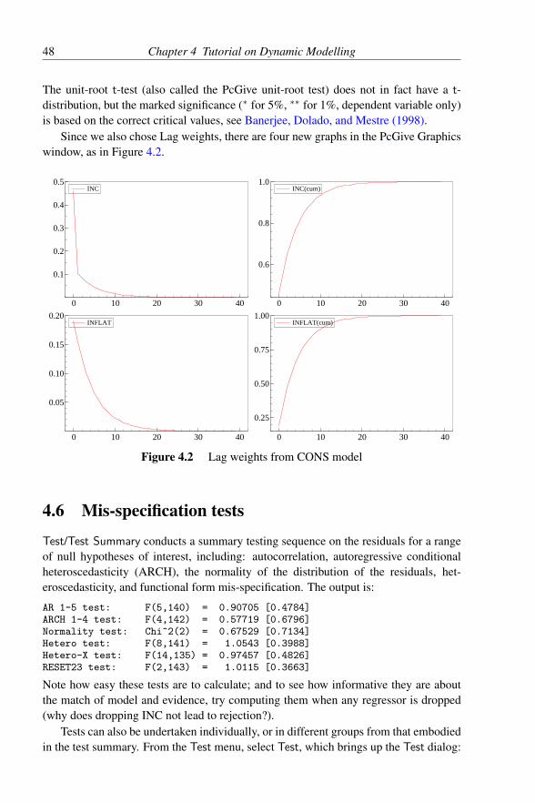
48 Chapter 4 Tutorial on Dynamic Modelling
The unit-root t-test (also called the PcGive unit-root test) does not in fact have a t-distribution, but the marked significance (∗ for 5%, ∗∗ for 1%, dependent variable only)is based on the correct critical values, see Banerjee, Dolado, and Mestre (1998).
Since we also chose Lag weights, there are four new graphs in the PcGive Graphicswindow, as in Figure 4.2.
INC
0 10 20 30 40
0.1
0.2
0.3
0.4
0.5INC INC(cum)
0 10 20 30 40
0.6
0.8
1.0INC(cum)
INFLAT
0 10 20 30 40
0.05
0.10
0.15
0.20INFLAT INFLAT(cum)
0 10 20 30 40
0.25
0.50
0.75
1.00INFLAT(cum)
Figure 4.2 Lag weights from CONS model
4.6 Mis-specification tests
Test/Test Summary conducts a summary testing sequence on the residuals for a rangeof null hypotheses of interest, including: autocorrelation, autoregressive conditionalheteroscedasticity (ARCH), the normality of the distribution of the residuals, het-eroscedasticity, and functional form mis-specification. The output is:
AR 1-5 test: F(5,140) = 0.90705 [0.4784]ARCH 1-4 test: F(4,142) = 0.57719 [0.6796]Normality test: Chi^2(2) = 0.67529 [0.7134]Hetero test: F(8,141) = 1.0543 [0.3988]Hetero-X test: F(14,135) = 0.97457 [0.4826]RESET23 test: F(2,143) = 1.0115 [0.3663]
Note how easy these tests are to calculate; and to see how informative they are aboutthe match of model and evidence, try computing them when any regressor is dropped(why does dropping INC not lead to rejection?).
Tests can also be undertaken individually, or in different groups from that embodiedin the test summary. From the Test menu, select Test, which brings up the Test dialog:

4.6 Mis-specification tests 49
Any or all available tests can be selected.Tip The default values for the lag length of the AR and ARCH tests are based on the
data frequency and the sample size. Different lag lengths can be selected in the Test
dialog.The output is rather more extensive than with batch tests. For example, the error auto-correlation test (or AR test) and ARCH test produce:
Error autocorrelation coefficients in auxiliary regression:Lag Coefficient Std.Error
1 0.054381 0.09092 0.071683 0.089873 -0.088316 0.087684 0.12258 0.088565 -0.051648 0.0885
RSS = 162.605 sigma = 1.16146
Testing for error autocorrelation from lags 1 to 5Chi^2(5) = 4.7067 [0.4527] and F-form F(5,140) = 0.90705 [0.4784]
ARCH coefficients:Lag Coefficient Std.Error
1 -0.065174 0.083992 -0.077844 0.083883 0.063463 0.083944 0.034848 0.08416
RSS = 345.559 sigma = 1.55997
Testing for error ARCH from lags 1 to 4ARCH 1-4 test: F(4,142) = 0.57719 [0.6796]
The DW -statistic (Durbin–Watson) was part of the standard output of PcGive up toversion 12. Now DW can be printed from the first entry on the Test dialog. But note

50 Chapter 4 Tutorial on Dynamic Modelling
that the assumptions needed to justify the application of the DW test in economics arerarely satisfied.
Similarly, the normality test leads to the low-order moments being reported. Thedensity of the scaled residuals was shown in Figure 4.1 and revealed slight skewnessand somewhat fatter tails than the standard normal distribution. These mis-specificationtest outcomes are satisfactory, consistent with the equation being a congruent model, sowe now consider some specification tests.
Note that you can use Test/Store to store residuals and fitted values from the regres-sion in the OxMetrics database.
4.7 Specification tests
4.7.1 Exclusion, linear and general restrictions
First, we test whether a subset of the coefficients is zero. Choose Exclusion Restrictions
from the Test menu to test whether one or more coefficients are zero. At the dialog markINC and INC 1 and accept:
Before looking at the subset test result, we shall also do a linear restrictions test onhomogeneity of CONS with respect to INC. This time, select Linear Restrictions. Tocomplete, edit the restrictions as follows:

4.7 Specification tests 51
This formulates one restriction. The last element is the r vector, specifying whatthe restriction should add up to. In terms of (4.1) the restrictions are:
(1 0 1 1 0)
a1
c
b0b1γ
= a1 + b0 + b1 = 1.
One further way of implementing this test is in the form of general restrictions.These are expressed as f(θ) = 0. Complete the dialog as follows, and accept:
The results of the three tests are:Test for excluding:[0] = INC[1] = INC_1Subset F(2,145) = 155.67 [0.0000]**
Test for linear restrictions (Rb=r):R matrix
CONS_1 Constant INC INC_1 INFLAT1.0000 0.00000 1.0000 1.0000 0.00000
r vector1.0000
LinRes F(1,145) = 4.0348 [0.0464]*
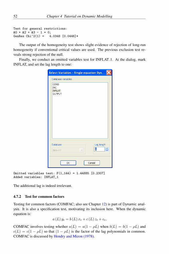
52 Chapter 4 Tutorial on Dynamic Modelling
Test for general restrictions:&0 + &2 + &3 - 1 = 0;GenRes Chi^2(1) = 4.0348 [0.0446]*
The output of the homogeneity test shows slight evidence of rejection of long-runhomogeneity if conventional critical values are used. The previous exclusion test re-veals strong rejection of the null.
Finally, we conduct an omitted variables test for INFLAT 1. At the dialog, markINFLAT, and set the lag length to one:
Omitted variables test: F(1,144) = 1.44885 [0.2307]Added variables: INFLAT_1
The additional lag is indeed irrelevant.
4.7.2 Test for common factors
Testing for common factors (COMFAC; also see Chapter 12) is part of Dynamic anal-
ysis. It is also a specification test, motivating its inclusion here. When the dynamicequation is:
a (L) yt = b (L)xt + c (L) zt + εt,
COMFAC involves testing whether a(L) = a(1 − ρL) when b(L) = b(1 − ρL) andc(L) = c(1 − ρL) so that (1 − ρL) is the factor of the lag polynomials in common.COMFAC is discussed by Hendry and Mizon (1978).

4.8 Options 53
To select COMFAC tests, the minimum lag length must be unity for all non-redundant variables (variables that are redundant when lagged can occur without lags:PcGive notices the Constant and Trend if such terms occur). First, we must revise themodel to have one lag on INFLAT: select the Model Formulation dialog, mark INFLATin the database, and add it to the model using a lag length of one. PcGive notices thatcurrent INFLAT is already in the model and doesn’t add it a second time. Estimateover the previously selected sample (the full sample, with 8 forecasts). Now select Dy-
namic analysis, and mark Test for common factors. Since the lag polynomials arefirst-order, only the Wald test of one common-factor restriction is presented followingthe roots of the lag polynomials. Here the restriction is rejected so the dynamics do nothave an autoregressive error representation, matching the very different roots of the lagpolynomials. The output is:
COMFAC Wald test table, COMFAC F(2,144) = 51.3999 [0.0000] **Order Cumulative tests Incremental tests1 Chi^2(2) = 102.8 [0.0000]** Chi^2(2) = 102.8 [0.0000]**
The remainder of this chapter uses the model without lagged INFLAT, so re-estimatethe previous model (still with 8 static forecasts).
4.8 Options
The Options entry on the OxMetrics Model dialog allow you to control the settingsfor iterative maximization (which we have not used yet), and select additional outputoptions.
The options related to maximization appear in the top part of the dialog:
Increasing the amount of iteration output could be useful if you wish to find out whya iterative maximization goes wrong.
Clicking on Additional reporting in the Options dialog expands the remainder ofthe dialog:

54 Chapter 4 Tutorial on Dynamic Modelling
The Test Summary is switched on by default (and can be switched off here if youdo not wish that), all the others are switched off. Marking any of these items will resultin the output automatically appearing after estimation. All Options settings are savedbetween runs of PcGive. Note however, that all these items are also available on demandfrom the Test menu.
4.9 Further OutputOther output formats may prove more convenient for direct inclusion in final reports.To make PcGive write the output in equation format, for example, activate the Further
Output, (on the Test menu) and mark as shown:
Reporting only the equation format, this produces:CONS = 0.8091*CONS_1 - 18.52 + 0.5067*INC - 0.2965*INC_1 - 0.9926*INFLAT(SE) (0.0255) (8.73) (0.0288) (0.0356) (0.0862)

4.10 Forecasting 55
4.10 Forecasting
To end this chapter, we briefly compare dynamic and static forecasts for this model.When we started, 8 observations were kept for static (1-step) forecasts, and these werelisted in §4.3.2 and graphed in Fig. 4.1d.
To replicate the results of §4.3.2, activate Test/Forecast (or click on the forecasticon on the toolbar). In the subsequent dialog, select the h-step forecasts radio button(keeping h = 1). Also set Forecast standard errors to use With parameter uncertainty:
The output appears in the in Forecasts graphics window, as well as the OxMetricsresults window. The latter matches that listed in §4.3.2; for the summary measures:
mean(Error) = -0.38151 RMSE = 1.1616SD(Error) = 1.0972 MAPE = 0.11129
The numbers are as before, but two additional statistics are reported. The first is theRoot Mean Square Error:
RMSE =
[1
H
H∑t=1
(yt − ft)2
]1/2
,
where the forecast horizon is H (8 here), yt the actual values, and ft the forecasts. The
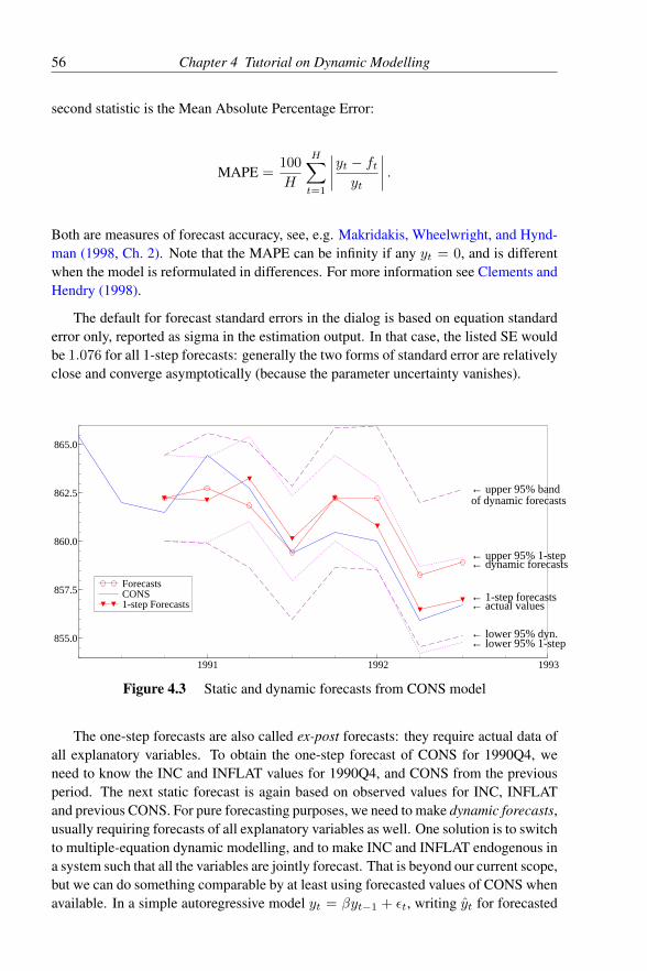
56 Chapter 4 Tutorial on Dynamic Modelling
second statistic is the Mean Absolute Percentage Error:
MAPE =100
H
H∑t=1
∣∣∣∣yt − ftyt
∣∣∣∣ .Both are measures of forecast accuracy, see, e.g. Makridakis, Wheelwright, and Hynd-man (1998, Ch. 2). Note that the MAPE can be infinity if any yt = 0, and is differentwhen the model is reformulated in differences. For more information see Clements andHendry (1998).
The default for forecast standard errors in the dialog is based on equation standarderror only, reported as sigma in the estimation output. In that case, the listed SE wouldbe 1.076 for all 1-step forecasts: generally the two forms of standard error are relativelyclose and converge asymptotically (because the parameter uncertainty vanishes).
Forecasts CONS 1-step Forecasts
1991 1992 1993
855.0
857.5
860.0
862.5
865.0
← actual values← 1-step forecasts
← upper 95% bandof dynamic forecasts
← lower 95% dyn.← lower 95% 1-step
← dynamic forecasts← upper 95% 1-step
Forecasts CONS 1-step Forecasts
Figure 4.3 Static and dynamic forecasts from CONS model
The one-step forecasts are also called ex-post forecasts: they require actual data ofall explanatory variables. To obtain the one-step forecast of CONS for 1990Q4, weneed to know the INC and INFLAT values for 1990Q4, and CONS from the previousperiod. The next static forecast is again based on observed values for INC, INFLATand previous CONS. For pure forecasting purposes, we need to make dynamic forecasts,usually requiring forecasts of all explanatory variables as well. One solution is to switchto multiple-equation dynamic modelling, and to make INC and INFLAT endogenous ina system such that all the variables are jointly forecast. That is beyond our current scope,but we can do something comparable by at least using forecasted values of CONS whenavailable. In a simple autoregressive model yt = βyt−1 + εt, writing yt for forecasted

4.10 Forecasting 57
values, and assuming that T + 1 is the first forecast period:
Forecast horizon Static Forecast Dynamic ForecastT + 1 yT+1 = βyT yT+1 = βyTT + 2 yT+2 = βyT+1 yT+2 = βyT+1
T + 3 yT+3 = βyT+2 yT+3 = βyT+2
The first forecast is the same, but thereafter the forecasts differ.
In the next chapter we consider strategies for model reduction, and the facilities thatPcGive offers to the applied modeller. This is followed by a chapter on automatic modelreduction — an important new addition to our toolbox and a major time-saving device.

Chapter 5
Tutorial on Model Reduction
5.1 The problems of simple-to-general modellingWhile the models used above were mainly selected as illustrations of the use of PcGive,they actually highlighted four important issues:1. Powerful tests can reveal model inadequacies: it is not sensible to skip testing in the
hope that the model is valid.2. A reject outcome on any test invalidates all earlier inferences, rendering useless the
time spent up to then – empirical research becomes highly inefficient if done thatway.
3. Once a problem is revealed by a test, how do you proceed? It is a dangerous nonsequitur to adopt the alternative hypothesis of the test which rejected: did you nearlydo this with residual autocorrelation, by assuming it was error autoregression andlooking for Cochrane–Orcutt [that is, RALS here]?
4. What can be done if two or more statistics reject? Which has caused what? Do bothor only one need to be corrected? Or should third factors be sought?As discussed in Chapters 12 and 14, the whole paradigm of postulating a simple
model and seeking to generalize it in the light of test rejections or anomalies is suspect,and in fact makes sub-optimal use of PcGive’s structure and functioning. Let us nowswitch to its mode of general-to-specific modelling.
5.2 Formulating general modelsWe wish to start this chapter with a clean modelling sheet. So exit PcGive and re-enterif you want your model numbering to coincide with the output presented in this chapter.
Turn to the formulation dialog to create a completely new, general specification. Insubstantive research, the starting point should be based on previous empirical researchevidence (to test in due course that earlier findings are parsimoniously encompassed),economic (or other relevant subject matter) theory, institutional knowledge, the datafrequency – and common sense. Here, we base the initial model on Davidson, Hendry,
58

5.3 Analyzing general models 59
Srba, and Yeo (1978) (denoted DHSY below) and begin by formulating an equationwith CONS, INC, INFLAT and Constant as its basic variables (you could add in OUT-PUT too if you like, but logic suggests it should be irrelevant given income).
Choose CONS, INC, and INFLAT with two lags each: please note that we are stillonly illustrating – in practice, five lags would be a better initial lag length for quarterlydata, but in a tutorial, the mass of detail could swamp the principles if we reported allthe numbers for a long lag length. Do not retain any forecasts for this run and select fullsample OLS:
EQ( 1) Modelling CONS by OLS (using data.in7)The estimation sample is: 1953(3) - 1992(3)
Coefficient Std.Error t-value t-prob Part.R^2CONS_1 0.823338 0.08223 10.0 0.000 0.4038CONS_2 -0.0315462 0.07151 -0.441 0.660 0.0013Constant -20.7434 9.070 -2.29 0.024 0.0341INC 0.500117 0.02922 17.1 0.000 0.6643INC_1 -0.295872 0.05568 -5.31 0.000 0.1602INC_2 0.0255575 0.04471 0.572 0.568 0.0022INFLAT -0.844115 0.2521 -3.35 0.001 0.0704INFLAT_1 -0.0801516 0.4348 -0.184 0.854 0.0002INFLAT_2 -0.137750 0.2633 -0.523 0.602 0.0018
sigma 1.09027 RSS 175.92662R^2 0.993857 F(8,148) = 2993 [0.000]**Adj.R^2 0.993524 log-likelihood -231.708no. of observations 157 no. of parameters 9mean(CONS) 875.78 se(CONS) 13.5487
Scan the output, noting the coefficient estimates en route (e.g. four t-values aresmall). Select the dynamic analysis to compute the static long-run solution:
Solved static long run equation for CONSCoefficient Std.Error t-value t-prob
Constant -99.6282 38.05 -2.62 0.010INC 1.10372 0.04237 26.0 0.000INFLAT -5.10074 0.5484 -9.30 0.000Long-run sigma = 5.23645
ECM = CONS + 99.6282 - 1.10372*INC + 5.10074*INFLAT;WALD test: Chi^2(2) = 981.088 [0.0000] **
Note the coefficient values (for example, INC is close to unity, INFLAT to −5) andtheir small standard errors (so INC is apparently significantly different from unity).
5.3 Analyzing general modelsThe analysis of the lag structure is now more interesting: the unit-root t-tests showthat the three basic variables matter as long-run levels (less so if very long lags wereselected initially), which rejects a lack of cointegration. The F-tests on the (whole)lag polynomials show that each also matters dynamically. However, lag length 2 is

60 Chapter 5 Tutorial on Model Reduction
irrelevant, whereas the first lag cannot be removed without a significant deterioration infit.
Analysis of lag structure, coefficients:Lag 0 Lag 1 Lag 2 Sum SE(Sum)
CONS -1 0.823 -0.0315 -0.208 0.0322Constant -20.7 0 0 -20.7 9.07INC 0.5 -0.296 0.0256 0.23 0.038INFLAT -0.844 -0.0802 -0.138 -1.06 0.132
Tests on the significance of each variableVariable F-test Value [ Prob] Unit-root t-testCONS F(2,148) = 306.93 [0.0000]** -6.4716**Constant F(1,148) = 5.2302 [0.0236]*INC F(3,148) = 102.74 [0.0000]** 6.0458INFLAT F(3,148) = 32.254 [0.0000]** -8.039
Tests on the significance of each lagLag 2 F(3,148) = 0.17158 [0.9155]Lag 1 F(3,148) = 38.745 [0.0000]**
Tests on the significance of all lags up to 2Lag 2 - 2 F(3,148) = 0.17158 [0.9155]Lag 1 - 2 F(6,148) = 207.76 [0.0000]**
These four perspectives on the model highlight which reductions are consistent withthe data, although they do not tell you in what order to simplify. That issue can beresolved in part by more experienced researchers (for one example see the discussionin Hendry, 1987). For the moment, we will follow a sequential simplification route,although generally it is better to transform to near orthogonality prior to simplification.
Can we trust the tests just viewed? The natural attack on that issue is to test all ofthe congruency requirements listed in the Help: so test using the test summary. Manyof these tests will already have been conducted during earlier tutorials. The residualplot looks normal, and no test rejects, although either of the autocorrelation or RESETtests suggests a possible problem may be lurking in the background (the former optiongives significant negative autocorrelation possibly owing to overfitting – keep an eyeon how that evolves as simplification proceeds). COMFAC accepts that one commonfactor can be extracted (matching the insignificant 2nd order lag, which would implythat the common factor had a coefficient of zero) but strongly rejects extracting two.The omitted variables test reveals that OUTPUT is indeed irrelevant. And the linearrestrictions test confirms that long-run homogeneity of CONS with respect to INC isrejected at the 5% level. Tentatively, therefore, we accept the general or statisticalmodel as data-congruent, with no need for the second lag.
AR 1-5 test: F(5,143) = 2.1861 [0.0589]ARCH 1-4 test: F(4,149) = 1.0123 [0.4030]Normality test: Chi^2(2) = 1.6495 [0.4384]Hetero test: F(16,140) = 0.74629 [0.7425]Hetero-X test: F(44,112) = 0.80959 [0.7843]RESET23 test: F(2,146) = 2.3183 [0.1021]
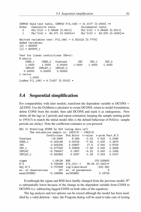
5.4 Sequential simplification 61
COMFAC Wald test table, COMFAC F(4,148) = 21.0177 [0.0000] **Order Cumulative tests Incremental tests2 Chi^2(2) = 0.39429 [0.8211] Chi^2(2) = 0.39429 [0.8211]1 Chi^2(4) = 84.071 [0.0000]** Chi^2(2) = 83.676 [0.0000]**
Omitted variables test: F(2,146) = 0.252122 [0.7775]Added variables:[0] = OUTPUT[1] = OUTPUT_1
Test for linear restrictions (Rb=r):R matrix
CONS_1 CONS_2 Constant INC INC_1 INC_21.0000 1.0000 0.00000 1.0000 1.0000 1.0000INFLAT INFLAT_1 INFLAT_2
0.00000 0.00000 0.00000r vector
1.0000LinRes F(1,148) = 4.71427 [0.0315] *
5.4 Sequential simplification
For comparability with later models, transform the dependent variable to DCONS =
∆CONS. Use the OxMetrics calculator to create DCONS, return to model formulation,delete CONS from the model, then add DCONS and mark it as endogenous. Nowdelete all the lags at 2 periods and repeat estimation, keeping the sample starting pointto 1953(3) to match the initial model (this is the default behaviour of PcGive: sampleperiods are sticky). Note the coefficient estimates as you proceed:
EQ( 2) Modelling DCONS by OLS (using data.in7)The estimation sample is: 1953(3) - 1992(3)
Coefficient Std.Error t-value t-prob Part.R^2Constant -19.9390 8.584 -2.32 0.022 0.0345CONS_1 -0.202149 0.02725 -7.42 0.000 0.2670INC 0.500235 0.02857 17.5 0.000 0.6700INC_1 -0.277320 0.03808 -7.28 0.000 0.2599INFLAT -0.784047 0.1857 -4.22 0.000 0.1056INFLAT_1 -0.262993 0.2057 -1.28 0.203 0.0107
sigma 1.08126 RSS 176.538482R^2 0.765599 F(5,151) = 98.64 [0.000]**Adj.R^2 0.757838 log-likelihood -231.981no. of observations 157 no. of parameters 6mean(DCONS) -0.189886 se(DCONS) 2.19724
Eventhough the sigma and RSS have hardly changed from the previous model, R2
is substantially lower because of the change in the dependent variable from CONS toDCONS (i.e. subtracting lagged CONS on both sides of the equation).
The lag analysis and test options can be reused although the model has been mod-ified by a valid deletion – later, the Progress dialog will be used to take care of testing

62 Chapter 5 Tutorial on Model Reduction
the validity of reductions. Using test summaries, few keystrokes or mouse clicks areneeded to completely re-estimate, regraph and retest the simplified model. Now theapparent residual autocorrelation has gone, suggesting that the earlier interpretation ofoverfitting was valid. RESET, too, is a little better. After testing whatever hypothesesare desired, select Progress on the OxMetrics Model dialog. A dialog appears, listingall the estimated models:
To offer a default sequence, PcGive decides that model A could be nested in modelB if the following conditions hold:• model A must have a lower log-likelihood (i.e. higher RSS),• model A must have fewer parameters,• model A and B must have the same sample period and database.
PcGive does not check if the same variables are involved, because transformations couldhide this. As a consequence PcGive does not always get the correct nesting sequence,and it is the user’s responsability to ensure nesting.
There are two options on the dialog:• Mark Specific to General
Marks more general models, finding a nesting sequence with strictly increasing log-likelihood.• Mark General to Specific
Marks all specific models that have a lower log-likelihood.The default selection is found by first setting the most recent model as specific, and thensetting the general model that was found as the general model. In this case, PcGive hasmarked both models,
Press OK to see the progress output:

5.4 Sequential simplification 63
Progress to dateModel T p log-likelihood SC HQ AICEQ( 1) 157 9 OLS -231.70831 3.2415 3.1375 3.0663EQ( 2) 157 6 OLS -231.98086 3.1484< 3.0790< 3.0316<
Tests of model reduction(please ensure models are nested for test validity)EQ( 1) --> EQ( 2): F(3,148) = 0.17158 [0.9155]
T is the number of observations, and p the number of esstimated parameters. This isfollowed by the estimation procedure (OLS here) and the log-likelihood. Finally, threeinformation criteria are listed: SC (Schwarz criterion), HQ (Hannan–Quinn) and AIC(Akaike information criterion). The F-test is the likelihood-ratio test for deleting all2-lagged variables.
Next, we will transform the model to a more interpretable specification, similar toDHSY. Bring up the calculator to transform the variables to sustain a new model of theform:
∆CONSt = β0 + β1∆INCt + β2(INC− CONS)t−1 + β3INFLATt
+β4INCt−1 + β5INFLATt−1.
Create (INC-CONS) by subtracting CONS from INC; call it SAVING, These new vari-ables need to be added to the model: add DINC and SAVING with one lag. Then INC,current SAVING and CONS 1 (or INC 1) must be deleted. Note that it is exactly thesame model as model 2 but with a different parametrization and hence a different extentof collinearity (see Chapter 15). Therefore, there is no need to re-estimate this model.But note in the previous output that INFLAT 1 is insignificant, so delete INFLAT 1to retain only DCONS, Constant, DINC, SAVING 1, INFLAT and INC 1 (that is, 5regressors). Estimate over the same sample period as previous models, to get model 3:EQ( 3) Modelling DCONS by OLS (using data.in7)
The estimation sample is: 1953(3) - 1992(3)
Coefficient Std.Error t-value t-prob Part.R^2Constant -19.6232 8.598 -2.28 0.024 0.0331DINC 0.507352 0.02808 18.1 0.000 0.6823SAVING_1 0.188689 0.02519 7.49 0.000 0.2696INC_1 0.0205447 0.009459 2.17 0.031 0.0301INFLAT -0.994858 0.08552 -11.6 0.000 0.4710
sigma 1.08352 RSS 178.449873R^2 0.763061 F(4,152) = 122.4 [0.000]**no. of observations 157 no. of parameters 5
Test as before and return to check the reduction sequence (again acceptable). Note thegreater interpretability of the regression parameters in this differences and levels form;also note that the effect of INC 1 is small, but matching the earlier static long run, issignificantly different from zero when conventional critical values are used (but see,for example, Banerjee, Dolado, Galbraith, and Hendry, 1993 for an analysis). In fact,the DGP for CONS does have a long-run coefficient of unity for INC, so we will next

64 Chapter 5 Tutorial on Model Reduction
delete that variable (albeit anticipating a ‘significant’ reduction this time: in fact, INC isendogenous here, and given the number of tests we planned to use, a 1% level for eachwould be sensible so the deletion is not deleterious). Thus, delete INC 1, and go backthrough estimation and testing (note the greatly improved precision of the coefficientsestimates in exchange for the cost of an increase in the residual standard error). Againselect the nesting sequence in the Progress dialog.
All the diagnostic tests are acceptable from the test summary, and the Progressreport is:
Progress to dateModel T p log-likelihood SC HQ AICEQ( 1) 157 9 OLS -231.70831 3.2415 3.1375 3.0663EQ( 2) 157 6 OLS -231.98086 3.1484 3.0790 3.0316EQ( 3) 157 5 OLS -232.82621 3.1270 3.0692< 3.0296<EQ( 4) 157 4 OLS -235.22574 3.1253< 3.0791 3.0475
Tests of model reductionEQ( 1) --> EQ( 2): F(3,148) = 0.17158 [0.9155]EQ( 1) --> EQ( 3): F(4,148) = 0.53068 [0.7134]EQ( 1) --> EQ( 4): F(5,148) = 1.3565 [0.2441]
EQ( 2) --> EQ( 3): F(1,151) = 1.6349 [0.2030]EQ( 2) --> EQ( 4): F(2,151) = 3.1863 [0.0441]*
EQ( 3) --> EQ( 4): F(1,152) = 4.7180 [0.0314]*
At the 5% level, Model 4 is ‘significantly’ worse than both models 2 and 3 but notthan model 1; however, its SC is smaller (log T ≈ 5.0 here, so SC falls for all valuesof F less than about 5) and hence model selection depends in this sample on the choiceof criterion and the level of significance. All further reductions by elimination will besignificant, although other transformations plus reductions might prove successful: tryusing the ECM which imposes the long-run inflation coefficient as well.
Finally, the resulting model can be re-estimated by RLS to test recursively for pa-rameter constancy (actually, the above model is not fully congruent, and the anomalousresults are reflections of that, although the estimates are quite close to those used in theDGP, see Appendix A2). Figure 5.1 shows the graphical analysis of this final model,re-estimated with 12 forecasts.
Tip Until a data set is saved, all changes within a run are transient; thus, changes willnot be kept if you exit prior to saving your data. This is important if new transfor-mations have been created and so automatically added to the database. OxMetricswill enquire as you exit if you wish to save the data. If you forget to save the trans-formed data, you will still have a record of the transformations in the results file.You could then paste the code of the transformations to the Algebra editor, saveit and then load the algebra file to transform on each run. This economizes on
disk space for data storage, and if you alter the base data, transformed variables areeasily recreated.

5.5 Encompassing tests 65
DCONS Fitted
1960 1970 1980 1990-5
0
5 DCONS Fitted DCONS × Forecasts DCONS × Fitted
-5.0 -2.5 0.0 2.5 5.0
-5
0
5DCONS × Forecasts DCONS × Fitted
rDCONS (scaled) forc.error
1960 1970 1980 1990-2.5
0.0
2.5 rDCONS (scaled) forc.error DCONS 1-step Forecasts
1989 1990 1991 1992 1993-5
0
5DCONS 1-step Forecasts
rDCONS N(0,1)
-2 0 2 4
0.2
0.4
DensityrDCONS N(0,1) ACF-rDCONS
0 5 10
0
1ACF-rDCONS
Figure 5.1 Graphical statistics for the final model with 12 forecasts
5.5 Encompassing tests
The final necessary condition is to ensure that the empirical model which was obtainedin the previous section is in the set of useful contenders, i.e. it is not dominated byany other model. More stringently, one might desire that no other model (M2 say)explained features of the data which one’s own model (M1) could not. This idea willbe formalized in §12.7.5 by encompassing (also see §14.7.6). We end this tutorial witha test for encompassing, which necessitates two non-nested models.
Start by regressing DCONS on CONS 1, INC, INC 1 and INFLAT 1, keeping thesample as before: 1953 (3) to 1992 (3). For the next model, delete INFLAT 1, addingINFLAT instead, and estimate. Then select Encompassing from the Test/Test dialog.The output comprises:
Encompassing test statistics: 1953(3) - 1992(3)
M1 is: DCONS onConstant CONS_1 INC INC_1 INFLAT_1
M2 is: DCONS onConstant CONS_1 INC INC_1 INFLAT
Instruments used:Constant CONS_1 INC INC_1 INFLAT_1INFLAT
sigma[M1] = 1.13957 sigma[M2] = 1.08352 sigma[Joint] = 1.08126
Test Model 1 vs. Model 2 Model 2 vs. Model 1

66 Chapter 5 Tutorial on Model Reduction
Cox N(0,1) = -5.039 [0.0000]** N(0,1) = -1.382 [0.1670]Ericsson IV N(0,1) = 4.407 [0.0000]** N(0,1) = 1.312 [0.1895]Sargan Chi^2(1) = 16.057 [0.0001]** Chi^2(1) = 1.6281 [0.2020]Joint Model F(1,151) = 17.835 [0.0000]** F(1,151) = 1.6349 [0.2030]
All the tests listed are automatically computed; none rejects model 2 and all rejectmodel 1 (see Chapter 12 for details). How many hours would that have taken with an-other program? And we have many tools yet untried to dig deeper into the performanceof econometric equations. Naturally you can extend, contract, transform or abandonyour model, switch sample period or estimation methods, save the model’s predictions,etc.
5.6 Model revisionIf you have made it this far, you can manage on your own for a bit. We hope youenjoyed doing empirical econometrics using PcGive and found it easy, powerful andfriendly to use. It is well worth reading through the econometrics Chapters 11–15. Youwill learn a great deal about the inadequacy of conventional methods when you seewhat you can investigate about claimed models. Indeed, you could now test your skillsagainst PcGive’s automatic selection algorithm discussed in the next chapter. Or readthe final tutorial chapter to delve further into non-linear models.

Chapter 6
Tutorial on Automatic Model Selectionusing Autometrics
6.1 IntroductionWe now turn to what is perhaps the most useful part of PcGive: automatic model selec-tion using Autometrics. The objective is to let the computer do a large part of what wasdone by hand in the previous chapter. PcGive will be able to find a model much quickerthan we can. Of course, there is always the option to do the model selection by hand —but it will be quite a challenge to beat Autometrics.
Autometrics is a computer implementation of general-to-specific modelling. Addi-tional information is provided in §12.6.5, §14.8, §15.10 and §15.11.
The starting point for Autometrics is a model formulated in the normal way. Thisinitial model is called the general unrestricted model or GUM. It should be a well-specified model, able to capture the salient features of the dependent variable and passall diagnostic tests. Following the GUM, the main decision is the significance level forreduction. This determines at what significance regressors are removed. It also specifiesthe extent to which we accept a deterioration in information relative to the GUM.
6.2 Modelling CONSIn §5.2 we shied away from using 5 lags to keep the model simple. Now we can be moreambitious, allowing for lags up to 5. Since the data is quarterly, we also add seasonals.In the previous chapter it was noted that OUTPUT should not matter. To investigatethis, we add it to the model as well. Finally, we add a trend, so that the formulated
67

68 Chapter 6 Tutorial on Automatic Model Selection using Autometrics
model is as follows:
Accept, then mark Autometrics, which activates the remainder of the dialog:• Target size
This is the significance level that is used for reduction. Change this to 0.05.• Outlier detection
Keep this at None. Alternative options are: Large residuals to automatically createdummies for large residuals in the GUM, and Dummy saturation to create dummiesfor all observations.
• Pre-search lag reduction
Pre-search lag reduction is switched on by default.• Advanced Autometrics settings
offers an additional dialog with advanced settings.• Use final model in next formulation dialog
When this is switched on (the default) the selected model will be the model for thenext formulation dialog. Otherwise it will be the GUM. The latter can be usefulwhen experimenting with different Autometrics settings.Note, however, that all actions in the Test menu relate to the final reduced model asfound by Autometrics. The choice here only applies to the default that is offered forthe next model.

6.2 Modelling CONS 69
Keep the remaining settings as shown here:
Press OK, and again in the next dialog which is unchanged from before (check thatyou’re using the full sample). Automatic model selection is quick, but generates moreoutput.• Initial GUM
First the GUM is printed. The output below is not how PcGive shows it. Instead wehave sorted the regressors by t-prob,1 i.e. by decreasing significance:
GUM( 1) Modelling CONS by OLSThe dataset is: .\OxMetrics7\data\data.in7The estimation sample is: 1954(2) - 1992(3)
Coefficient Std.Error t-value t-prob Part.R^2CONS_1 0.833937 0.08599 9.70 0.0000 0.4274CONS_2 0.0497580 0.1101 0.452 0.6522 0.0016CONS_3 -0.150692 0.1090 -1.38 0.1693 0.0149CONS_4 0.197144 0.1103 1.79 0.0762 0.0247CONS_5 -0.132990 0.07766 -1.71 0.0893 0.0227Constant -20.7235 22.88 -0.906 0.3667 0.0065INC 0.511109 0.03237 15.8 0.0000 0.6643INC_1 -0.312776 0.05848 -5.35 0.0000 0.1850INC_2 -0.0507675 0.06353 -0.799 0.4258 0.0050INC_3 0.120765 0.06381 1.89 0.0607 0.0276INC_4 -0.0396864 0.06536 -0.607 0.5448 0.0029INC_5 -0.00320849 0.05006 -0.0641 0.9490 0.0000INFLAT -0.766260 0.3703 -2.07 0.0405 0.0329INFLAT_1 0.113980 0.5978 0.191 0.8491 0.0003INFLAT_2 -0.511191 0.6022 -0.849 0.3975 0.0057INFLAT_3 -0.332742 0.5959 -0.558 0.5776 0.0025INFLAT_4 0.675374 0.5832 1.16 0.2490 0.0105INFLAT_5 -0.0770788 0.3298 -0.234 0.8156 0.0004OUTPUT -0.00695063 0.03279 -0.212 0.8324 0.0004OUTPUT_1 -0.00637418 0.05040 -0.126 0.8996 0.0001OUTPUT_2 -0.0247968 0.05115 -0.485 0.6287 0.0019
1 This can be done easily by selecting the column using the right mouse button, then right-clicking inside the selection, and using Sort.

70 Chapter 6 Tutorial on Automatic Model Selection using Autometrics
OUTPUT_3 0.0514746 0.05177 0.994 0.3220 0.0078OUTPUT_4 0.0398924 0.05253 0.759 0.4490 0.0046OUTPUT_5 -0.0542604 0.04381 -1.24 0.2178 0.0120Seasonal 0.234970 0.2676 0.878 0.3815 0.0061Seasonal_1 0.213602 0.2768 0.772 0.4418 0.0047Seasonal_2 0.190405 0.2738 0.696 0.4880 0.0038Trend -0.000643632 0.004692 -0.137 0.8911 0.0001
sigma 1.08642 RSS 148.719356R^2 0.994754 F(27,126) = 884.8 [0.000]**Adj.R^2 0.993629 log-likelihood -215.83no. of observations 154 no. of parameters 28mean(CONS) 875.591 se(CONS) 13.6115
AR 1-5 test: F(5,121) = 0.66157 [0.6533]ARCH 1-4 test: F(4,146) = 1.6523 [0.1643]Normality test: Chi^2(2) = 2.3692 [0.3059]Hetero test: F(51,102)= 0.97127 [0.5369]Chow test: F(45,81) = 1.2000 [0.2354] for break after 1981(2)
The first four form the core model we have worked with so far. The remaining 24appear to be insignificant at 5%, but some may well survive into the final model. TheGUM is followed by the output of the diagnostic tests that are used by Autometrics.• Dimensions
Next is some information regarding the size of the problem:---------- Autometrics: dimensions of initial GUM ----------no. of observations 154 no. of parameters 28no. free regressors (k1) 28 no. free components (k2) 0no. of equations 1 no. diagnostic tests 5
• 0.2 Pre-search lag reductionThe first stage of the automatic model selection is the pre-search lag reduction:[0.2] Presearch reduction of initial GUM
Starting closed lag reduction at 0.33365Removing lags(#regressors): none
Starting common lag reduction at 0.33365Removing lags(#regressors): 2(4)
Starting common lag reduction at 0.33365 (excluding lagged y’s)Removing lags(#regressors): 5(3) 4(3)
Presearch reduction in opposite order
Starting common lag reduction at 0.33365 (excluding lagged y’s)Removing lags(#regressors): 4(3) 2(3) 5(3)
Starting common lag reduction at 0.33365Removing lags(#regressors): 2(1)
Starting closed lag reduction at 0.33365Removing lags(#regressors): none

6.2 Modelling CONS 71
Encompassing test against initial GUM (iGUM) removes: none
Presearch reduction: 10 removed, LRF_iGUM(10) [0.8430]Presearch removed:[0] = CONS_2[1] = INC_2[2] = INC_4[3] = INC_5[4] = INFLAT_2[5] = INFLAT_4[6] = INFLAT_5[7] = OUTPUT_2[8] = OUTPUT_4[9] = OUTPUT_5
The pre-search lag reduction is done in two sequences. Only lags that are insignif-icant in both (at a reduced level) are removed from the initial GUM. All tests areF-tests, derived from the likelihood-ratio (LR) test — they are the standard F-tests.Lag 2, which has four variables (seasonals are not treated as lags), is the least signif-icant with a p-value of 79%. In this case, both sequences remove exactly the sameregressors, so 10 terms are removed in the pre-search, leaving 18 coefficients.The advanced options make it possible to print the full trace output. This tends tobe very long. For the lag presearch it would print:[0.2] Presearch reduction of initial GUM
Starting closed lag reduction at 0.33365Trying all at lag 5 LRF( 4) [0.0700] kept
Starting common lag reduction at 0.33365Testing all at lag 5 LRF( 4) [0.0700]Testing all at lag 4 LRF( 4) [0.1711]Testing all at lag 3 LRF( 4) [0.1942]Testing all at lag 2 LRF( 4) [0.7912]Testing all at lag 1 LRF_min [0.0000]Testing all at lag 0 LRF_min [0.0000]Trying all at lag 2 LRF( 4) [0.7912] 4 removed
Starting common lag reduction at 0.33365 (excluding lagged y’s)Testing all at lag 5 LRF( 3) [0.7033] LRF_iGUM( 7)[0.8751]Testing all at lag 4 LRF( 3) [0.6496] LRF_iGUM( 7)[0.8524]Testing all at lag 3 LRF( 3) [0.1177] LRF_iGUM( 7)[0.3784]Testing all at lag 1 LRF_min [0.0000]Testing all at lag 0 LRF_min [0.0000]Trying all at lag 5 LRF( 3) [0.7033] LRF_iGUM( 7)[0.8751] 3 removedTrying all at lag 4 LRF( 3) [0.4596] LRF_iGUM(10)[0.8430] 3 removed
Presearch reduction in opposite order
Starting common lag reduction at 0.33365 (excluding lagged y’s)Testing all at lag 5 LRF( 3) [0.6377]Testing all at lag 4 LRF( 3) [0.6657]Testing all at lag 3 LRF( 3) [0.1172]Testing all at lag 2 LRF( 3) [0.6603]
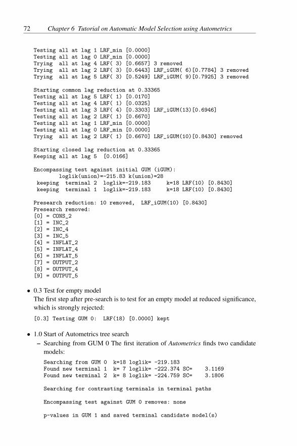
72 Chapter 6 Tutorial on Automatic Model Selection using Autometrics
Testing all at lag 1 LRF_min [0.0000]Testing all at lag 0 LRF_min [0.0000]Trying all at lag 4 LRF( 3) [0.6657] 3 removedTrying all at lag 2 LRF( 3) [0.6443] LRF_iGUM( 6)[0.7784] 3 removedTrying all at lag 5 LRF( 3) [0.5249] LRF_iGUM( 9)[0.7925] 3 removed
Starting common lag reduction at 0.33365Testing all at lag 5 LRF( 1) [0.0170]Testing all at lag 4 LRF( 1) [0.0325]Testing all at lag 3 LRF( 4) [0.3303] LRF_iGUM(13)[0.6946]Testing all at lag 2 LRF( 1) [0.6670]Testing all at lag 1 LRF_min [0.0000]Testing all at lag 0 LRF_min [0.0000]Trying all at lag 2 LRF( 1) [0.6670] LRF_iGUM(10)[0.8430] removed
Starting closed lag reduction at 0.33365Keeping all at lag 5 [0.0166]
Encompassing test against initial GUM (iGUM):loglik(union)=-215.83 k(union)=28
keeping terminal 2 loglik=-219.183 k=18 LRF(10) [0.8430]keeping terminal 1 loglik=-219.183 k=18 LRF(10) [0.8430]
Presearch reduction: 10 removed, LRF_iGUM(10) [0.8430]Presearch removed:[0] = CONS_2[1] = INC_2[2] = INC_4[3] = INC_5[4] = INFLAT_2[5] = INFLAT_4[6] = INFLAT_5[7] = OUTPUT_2[8] = OUTPUT_4[9] = OUTPUT_5
• 0.3 Test for empty modelThe first step after pre-search is to test for an empty model at reduced significance,which is strongly rejected:
[0.3] Testing GUM 0: LRF(18) [0.0000] kept
• 1.0 Start of Autometrics tree search– Searching from GUM 0 The first iteration of Autometrics finds two candidate
models:Searching from GUM 0 k=18 loglik= -219.183Found new terminal 1 k= 7 loglik= -222.374 SC= 3.1169Found new terminal 2 k= 8 loglik= -224.759 SC= 3.1806
Searching for contrasting terminals in terminal paths
Encompassing test against GUM 0 removes: none
p-values in GUM 1 and saved terminal candidate model(s)

6.2 Modelling CONS 73
GUM 1 terminal 1 terminal 2CONS_1 0.00000000 0.00000000 0.00000000CONS_4 0.02277320 0.02115435 0.02428157CONS_5 0.00375999 0.00183605 0.01389229Constant 0.34209071 0.04299342 .INC 0.00000000 0.00000000 0.00000000INC_1 0.00000000 0.00000000 0.00000000INFLAT 0.02066361 0.00000000 .INFLAT_1 0.34251808 . 0.00000000OUTPUT_1 0.39200132 . 0.00004627OUTPUT_3 0.45148458 . 0.01234609k 10 7 8parameters 10 7 8loglik -221.84 -222.37 -224.76AIC 3.0109 2.9789 3.0228HQ 3.0910 3.0350 3.0869SC 3.2081 3.1169 3.1806
=======
– Searching from GUM 1, terminationGUM 1 is the starting point for the next search. This does not produce any newterminal candidates:Searching from GUM 1 k=10 loglik= -221.840 LRF_GUM0(8)[0.7792]Recalling terminal 1 k= 7 loglik= -222.374 SC= 3.1169Recalling terminal 2 k= 8 loglik= -224.759 SC= 3.1806
Searching for contrasting terminals in terminal paths
• 2.0 Selection of final model from terminal candidates: terminal 1Because there were no new models when searching from GUM 1, the table headed‘p-values in Final GUM and terminal model(s)’ is the same as that reported aftersearching from GUM 0, except that now the column of terminal one is marked. Theselected model has the lowest Schwarz Criterion (SC), which is terminal 1 here.Before printing the final model, the output includes the coefficients, diagnostic testsand a summary of the search:
coeffs and diagnostic p-values in Final GUM and terminal model(s)Final GUM terminal 1 terminal 2
CONS_1 0.79408 0.80973 0.77254CONS_4 0.12045 0.11861 0.12052CONS_5 -0.12270 -0.12922 -0.10247Constant -14.021 -17.144 .INC 0.50462 0.50414 0.50407INC_1 -0.27529 -0.28567 -0.25909INFLAT -0.71889 -1.0022 .INFLAT_1 -0.35764 . -1.1672OUTPUT_1 -0.026912 . -0.083022OUTPUT_3 0.021618 . 0.055266k 10 7 8parameters 10 7 8loglik -221.84 -222.37 -224.76sigma 1.0567 1.0495 1.0695AR(5) 0.82830 0.80906 0.69804

74 Chapter 6 Tutorial on Automatic Model Selection using Autometrics
ARCH(4) 0.23096 0.30509 0.12389Normality 0.50458 0.60556 0.40183Hetero 0.53356 0.65103 0.50246Chow(70%) 0.23208 0.19159 0.30902
=======
p-values of diagnostic checks for model validityInitial GUM cut-off Final GUM cut-off Final model
AR(5) 0.65329 0.01000 0.82830 0.01000 0.80906ARCH(4) 0.16430 0.01000 0.23096 0.01000 0.30509Normality 0.30587 0.01000 0.50458 0.01000 0.60556Hetero 0.53688 0.01000 0.53356 0.01000 0.65103Chow(70%) 0.23543 0.01000 0.23208 0.01000 0.19159
Summary of Autometrics searchinitial search space 2^28 final search space 2^10no. estimated models 119 no. terminal models 2test form LR-F target size Default:0.05outlier detection no presearch reduction lagsbacktesting GUM0 tie-breaker SCdiagnostics p-value 0.01 search effort standardtime 0.48 Autometrics version 1.5e
The final model, which differs from the one of the previous chapter, has lags fourand five of CONS (with almost opposite coefficients), as additional variables. Given 28variables in the GUM, at 5% significance one might expect one or two to be retainedby chance; a 1% level would reduce that ‘spurious’ retention rate to about one variableevery three times that such a selection exercise was conducted. Any actions on the Test
menu now relate to this model. For example, testing that the coefficients on CONS 4and CONS 5 sum to zero using Test/Linear Restrictions:
This is accepted with a p-value of 63%. Therefore, the long-run is not greatlychanged from that reported in §5.2:Solved static long-run equation for CONS
Coefficient Std.Error t-value t-probConstant -85.3400 37.66 -2.27 0.0249INC 1.08753 0.04200 25.9 0.0000INFLAT -4.98868 0.5069 -9.84 0.0000Long-run sigma = 5.22436

6.3 DHSY revisited 75
6.3 DHSY revisited
The DHSY model (Davidson, Hendry, Srba, and Yeo, 1978) is an equilibrium-correction model for the logarithm of consumption, ct, where the equilibrium correctionis the gap between consumption and income, yt, with an additional price term, ∆4pt.The DHSY model is seasonal: it uses fourth differences (the data are quarterly), and theequilibrium is towards the gap from a year ago. There is a dummy, Dbudget, for budgeteffects in 1968: +1 in 1968(1) and −1 in 1968(2), and a dummy, DVAT, for the intro-duction of VAT: +1 in 1973(1) and −1 in 1973(2). DHSY use DVt = Dbudget + DVAT
in their model:
∆4ct = −0.09(c− y)t−4 + 0.48∆4yt − 0.12∆4pt−0.23∆1∆4yt − 0.31∆1∆4pt + 0.006∆4DVt.
Load the DHSY.in7 data file from the OxMetrics7\data folder, and run DHSY.algwhich is in the algebra folder. Formulate the GUM with LC as the dependent variable,with up to 5 lags of LC, LY and D4LPC as explanatory variables. The constant isalready there, add the differenced dummy D4DV without further lags, and finally addthe seasonals. Estimation is over the sample period 1959(2)–1975(4).
Autometrics at 5% with pre-search lag reduction finds three terminal models:
Final GUM terminal 1 terminal 2 terminal 3LC_4 0.00000000 0.00000000 0.00000000 0.00000000Constant 0.25080661 . 0.07892034 .LY 0.00000000 0.00000000 0.00000000 0.00000000LY_1 0.00001040 0.00001130 0.00004104 0.00000567LY_4 0.12185243 0.00481955 . .LY_5 0.00005534 0.00000006 0.00003951 0.00000000D4LPC 0.00019983 0.00020981 0.00000000 0.00001474D4LPC_1 0.03371598 0.01494571 . 0.00933580D4DV 0.00190637 0.00201634 0.00059359 0.00027128Seasonal 0.04210896 . 0.00741163 .Seasonal_1 0.01466068 . 0.00017796 0.01432980Seasonal_2 0.07091657 . 0.01482352 .k 12 8 10 8parameters 12 8 10 8loglik 257.41 253.24 252.66 252.12AIC -7.3256 -7.3205 -7.2437 -7.2872HQ -7.1693 -7.2163 -7.1135 -7.1830SC -6.9307 -7.0573 -6.9147 -7.0239
=======
The selected model is very similar to that found by Davidson, Hendry, Srba, and

76 Chapter 6 Tutorial on Automatic Model Selection using Autometrics
Yeo (1978) (after much less effort than theirs!):
ct = 0.92(0.0284)
ct−4 + 0.268(0.0375)
yt + 0.194(0.0404)
yt−1
− 0.135(0.0462)
yt−4 − 0.246(0.0396)
yt−5 − 0.376(0.0951)
∆4pt
+ 0.252(0.101)
∆4pt−1 + 0.00695(0.00215)
∆4DVt
σ = 0.59%

Chapter 7
Tutorial on Estimation Methods
Three main groups of single equation dynamic modelling estimation methods will beexplained. The first is recursive estimation where we describe recursive least squaresin detail. Next, we examine instrumental variables estimation, then turn to estimatingmodels with autoregressive errors. That provides a convenient introduction to non-linear optimization and the tutorial concludes by considering non-linear least squaresmethods, which is a separate model class. Maximum likelihood estimation, which isalso is part of the non-linear modelling class, is considered in Chapter 9.
7.1 Recursive estimationFormulate a model consisting of CONS on Constant, CONS 1, INC and INC 1, asexplained in the previous chapter. Keep ordinary least squares in the Model Settings
dialog. Move to the model estimation dialog, set the maximum possible estimationsample, and keep 8 observations for forecasting. Now tick the Recursive estimation
box. Chapter 13 explains the algebra of recursive estimation; the logic is simply to fitthe model to an initial sample of M − 1 points and then fit the equation to samples ofM, M + 1, ... up to T observations. The main output will be graphs of coefficients, σetc. over the sample. This is a powerful way to study parameter constancy (especiallyin its absence!).
The number of observations for initialization (the M − 1 above) is set to 15 (to bechanged from the default of 10). Press the OK button to estimate. In a trice, all T −Mestimates and associated statistics are computed. The final (full sample) estimates areshown in the Results window.
The one new statistic reported to the Results window is for the mean of the innova-tions being zero. Here we have:1-step (ex post) forecast analysis 1990(4) - 1992(3)Parameter constancy forecast tests:Forecast Chi^2(8) = 7.505 [0.4833]Chow F(8,146) = 0.90149 [0.5171]CUSUM t(7) = -1.317 [0.2292] (zero forecast innovation mean)
77

78 Chapter 7 Tutorial on Estimation Methods
so that this test does not detect any non-constancy. Interestingly, neither do the insta-bility statistics (based on Hansen, 1992): select Test/Test and mark Instability tests forthe reported outcomes (significance would be marked by one or two stars):
Instability tests:variance 0.36720joint 1.0166Individual instability tests:CONS_1 0.21030Constant 0.20566INC 0.21021INC_1 0.21033
The main new option on the Test menu is the Recursive Graphics dialog. Activatethis:
The right column has all the variables to be plotted in beta coefficients and betat-values. Select the statistics which are to be plotted: beta coefficients, beta t-values,1-step residuals, and all three Chow tests. First, the graph of the coefficient of CONS 1over the sample in Figure 7.1 shows that after 1978, βt lies outside of the previousconfidence interval which an investigator pre-1974 would have calculated as the basisfor forecasting. Other coefficients are also non-constant. Further, the 1-step residualsshow major outliers around 1974.
The 1-step residuals are ut = yt − x′tβt and they are plotted with ±2σt shown oneither side of zero. Thus ut which are outside of the error bars are either outliers or areassociated with changes in σ. Note the increase in σt around 1974 (the oil crisis ...).The 1-step Chow tests amply reflects this. A further summary graph is the break-pointChow test graph. Each point is the value of the Chow F-test for that date against thefinal period, here 1990(3), scaled by its 1% critical value (which becomes the line atunity), so the forecast horizon N is decreasing from left to right (hence the name Ndntests). Figure 7.1 illustrates: the critical value can be set at any desired probability level.
Peruse other options as you wish: see how the standardized innovations often high-light the outliers, or how the residual sums of squares confirm that a break occurred

7.2 Instrumental variables 79
CONS_1 × +/-2SE
1960 1980
0.50
0.75
1.00
1.25CONS_1 × +/-2SE Constant × +/-2SE
1960 1980
-100
0
100
200Constant × +/-2SE INC × +/-2SE
1960 1980
0.4
0.6
0.8
1.0INC × +/-2SE
INC_1 × +/-2SE
1960 1980
-0.6
-0.4
-0.2INC_1 × +/-2SE t: CONS_1
1960 1980
10
20
30
40t: CONS_1 t: Constant
1960 1980
-1
0
1
2t: Constant
t: INC
1960 1980
7.5
10.0
12.5 t: INC t: INC_1
1960 1980
-10.0
-7.5
-5.0 t: INC_1 Res1Step
1960 1980
-2.5
2.5Res1Step
1up CHOWs 1%
1960 1980
1
2
31up CHOWs 1% Ndn CHOWs 1%
1960 1980
0.5
1.0
1.5Ndn CHOWs 1% Nup CHOWs 1%
1960 1980
0.25
0.50
0.75
1.00Nup CHOWs 1%
Figure 7.1 Recursive least squares graphical constancy statistics
in 1974. Any of these graphs can be edited and printed, or saved for later recall andprinting.
Next, select the Graphic analysis dialog and look at the full sample residuals:
ut = yt − x′tβT
where βT is the usual full-sample OLS estimate. The full-sample estimates somewhatsmooth the outliers evident in the recursive figures, so now the largest is not much morethan 3.5 standard errors (partly because σ increased by about 50% over the sample).
That completes RLS. Note that RLS can be used to check the constancy of pre-tests such as (Augmented) Dickey–Fuller tests for the order of integration of a timeseries, and the recursive graphs may help to discriminate between genuine unit rootsand autoregressive coefficients driven towards unity by a failure to model a regimeshift.
7.2 Instrumental variablesIn many situations it may not be legitimate to treat all regressors as valid conditioningvariables, hence instrumental variables (IV) (which for extraneous reasons are known tobe valid) must be used. Reselect Model/Formulate as a first step towards the IV option.To compute instrumental variables, PcGive needs to know the status (dependent – ornormalized – variable, endogenous, and exogenous or lagged) that you wish to assign toeach variable. Given the present model, with a predefined dependent variable (CONS),known lags (CONS 1, INC 1) and a known status for the Constant (exogenous, as it is

80 Chapter 7 Tutorial on Estimation Methods
deterministic), only INC needs a status. Thus, make INC endogenous: right click on itand select Y: endogenous as shown:
Next, the instruments must be selected. The lag polynomial choices for additionalinstruments must be sufficient to identify the equation: add OUTPUT with one lag tothe model. Highlight both in the model, and select A: additional instrument in thedrop-down box below the model, and press the Set button to mark these as Additionalinstruments. The model is now as shown above.
OK to accept and bring up the Model Settings dialog, if it is not already the default,switch to Instrumental variables, and press OK again. The available estimation methodis two-stage least squares (TSLS). Keep 8 observations for static forecasting.

7.2 Instrumental variables 81
7.2.1 Structural estimates
The structural estimates from the IV estimation appear in OxMetrics:
EQ( 3) Modelling CONS by IVE (using data.in7)The estimation sample is: 1953(2) - 1990(3)
Coefficient Std.Error t-value t-probINC Y 0.373349 0.1025 3.64 0.000CONS_1 1.01559 0.03633 28.0 0.000INC_1 -0.407460 0.07771 -5.24 0.000Constant 16.6558 14.38 1.16 0.249
sigma 1.53761 RSS 345.179245Reduced form sigma 2.0505no. of observations 150 no. of parameters 4no. endogenous variables 2 no. of instruments 5mean(CONS) 876.685 se(CONS) 13.3658Additional instruments:[0] = OUTPUT[1] = OUTPUT_1
Specification test: Chi^2(1) = 14.883 [0.0001]**Testing beta = 0: Chi^2(3) = 10986. [0.0000]**
1-step (ex post) forecast analysis 1990(4) - 1992(3)Forecast test: Chi^2(8) = 6.5087 [0.5904]
The specification χ2-test is for the validity of the instruments – and strongly rejects.Did you anticipate that? If so, which variables are the culprits? The χ2 (3) testingβ = 0 is the analogue of the OLS F-test of R2 equal to zero (so testing whether all thecoefficients except the constant term are zero). Note how the coefficient of CONS 1 islarger than unity. All of these counter indicators suggest serious mis-specification.
Next we test the model for other problems, similar to the approach and methodsused for least squares. The test summary produces:
AR 1-5 test: F(5,141) = 7.2440 [0.0000]**ARCH 1-4 test: F(4,142) = 7.5340 [0.0000]**Normality test: Chi^2(2) = 5.0900 [0.0785]Hetero test: F(6,143) = 1.1672 [0.3272]Hetero-X test: F(9,140) = 1.1480 [0.3334]
Note the significant residual autocorrelation, invalidating most of the inferences youmay have been tempted to make en route. The use of instrumental variables may correcta simultaneity or measurement error problem, but the basic model specification must besound before their use.
7.2.2 Reduced forms
The reduced form estimates are the regressions of each endogenous variable on theinstruments alone, so there are two equations (for CONS and INC). Select Test/Further
Output and mark Reduced form estimates. Press OK to see:

82 Chapter 7 Tutorial on Estimation Methods
Reduced form estimatesURF coefficients
CONS INCCONS_1 1.0171 0.023619INC_1 -0.079785 0.72756Constant 6.2285 -58.808OUTPUT 0.20994 0.26855OUTPUT_1 -0.16812 -0.032723
URF coefficient standard errorsCONS INC
CONS_1 0.046472 0.064342INC_1 0.050468 0.069875Constant 25.118 34.777OUTPUT 0.053144 0.073581OUTPUT_1 0.054809 0.075885
URF equation standard errorsCONS INC
2.0505 2.8390
correlation of URF residualsCONS INC
CONS 1.0000INC 0.73243 1.0000
If these reduced form equations fit badly (in terms of their σs), the IV estimateswill be poorly determined later. Note that these equations are unrestricted; once thestructural model (here CONS on CONS 1, INC, INC 1 and a Constant) is estimated, thereduced form equation for INC can be used to eliminate it from the structural equationto produce a restricted reduced form for CONS. Thus, a comparison of the unrestrictedand restricted reduced forms allows a test for the validity of the instruments (see Sargan,1964). This was shown with the structural estimates above: could you expect a good orbad outcome on such a test from what you have seen here?
Dynamic forecasting is not available for IVE. Instead, build a simultaneous equa-tions model using the multiple equation class, which allows dynamic forecasting fromsuch a model.
7.3 Autoregressive least squares (RALS)In this section we require the first difference of CONS. If you do not have this in thedatabase yet, switch to OxMetrics, and use the Calculator to create DCONS (or useAlgebra: DCONS = diff(CONS,1); ).
The following assumes that ∆CONS is the dependent variable and that the regres-sors are only Constant, CONS 1, INC and INC 1: if you do not wish to create DCONS,simply add unity to the coefficient of CONS 1 below; if any INFLAT variables remain,delete these.
To access RALS (rth order autoregressive least squares), check the Autoregressive
least squares option in the model settings dialog:

7.3 Autoregressive least squares (RALS) 83
You can also change the start and end lag order, but here we only estimate first order,which is the default. There is only one estimation option, Non-linear Estimation:
As usual, PcGive offers the sample period for your approval in the next dialog. Setit to 1953(3) - 1992(3), which is the maximum available sample, and use 8 forecasts.RALS requires lagged information for estimation. Here, one observation additionalis required: 1953(2); however, if you do not change the sample, PcGive will do itautomatically.
There is also a choice whether to do automatic estimation or not. Automatic max-imization will estimate the model directly, and is usually adequate. Non-automaticmaximization offers a dialog to control the iterative estimation process or for a gridsearch. Uncheck automatic maximization to see:

84 Chapter 7 Tutorial on Estimation Methods
The initial values for RALS are provided by OLS. The parameters are the coefficientsfrom OLS estimation, followed by an nth-order autoregressive error process (initializedby an LM-test, the order being set at the frequency+1, or the maximum lag length,whichever is smaller) and the function is minus the residual sum of squares divided bythe sample size T .
7.3.1 Optimization
The available options are:1. Choose the orders (s, r) of the error process:
ut =
r∑j=s
αjut−j + εt
This must be done in the model settings dialog.2. Coefficient values can be set to any particular desired value by double clicking on
the coefficient in the list box.3. Reset the initial values to those at dialog entry.4. Estimate, to optimize the objective function starting from the listed coefficient val-
ues.5. Press Options to control the maximization process:• Change the maximum number of iterations (that is, steps in which the function
value reduces); if this number is reached, the optimization process will abort,despite not finding the minimum yet.• Specify how often (if at all) iteration output is printed; and• Set the convergence criterion.
6. Conduct a Grid search over the model parameters, most importantly for the αi (la-belled Uhat 1,. . .Uhat p in the dialog).

7.3 Autoregressive least squares (RALS) 85
Begin with a grid, to view the graph of the function against the first-order autore-gressive parameter. The dialog allows you to select the region for the grid search, aswell as the resolution of the search. Press Grid, and select Uhat 1 in the parameter box.The grid center is automatically set to the current value of the parameter, 0.33045 . . .
here. Change the grid center to 0, the step size to 0.1, and select Maximize:
Set the Grid Options to Max: maximize over remaining parameters. With this option,we can read the actual maximum from the graph (and it is fast enough to use). PressNext Grid for a second grid, again for Uhat 1, but now centred on 0.9, in steps of 0.01.Press OK to compute and graph the grids.
The results are in Figure 7.2. There is a local maximum around 0.4, but the linegoes up again after 0.8. The second graph inspects the rightmost section of the grid:centred at 0.9. Use the point facility when the graph is on the screen (View/Point): amaximum of about −1.86 seems to be around 0.97. We can also do a more accurategrid around 0.4 and read the maximum off the screen. Centre the grid around 0.4 andselect a step length of 0.01. Here we find a minimum of −1.87 around 0.43 to 0.44.The optimum appears to be at 0.97, but the two minima have similar function values.
On completion of the grid, the RALS estimation dialog reappears. Now selectAlt+e for estimation. Note that iterations can be interrupted (for example, if too slowor diverging), but here convergence is achieved very rapidly. After convergence, theOK button lights up. Press OK to write the RALS output to the Results window.EQ( 1) Modelling DCONS by RALS (using data.in7)
The estimation sample is: 1953(3) - 1990(3)Coefficient Std.Error t-value t-prob Part.R^2
Constant -11.2824 18.52 -0.609 0.543 0.0026CONS_1 -0.101503 0.05330 -1.90 0.059 0.0246INC 0.505354 0.03716 13.6 0.000 0.5623INC_1 -0.393064 0.05540 -7.09 0.000 0.2590Uhat_1 0.436339 0.09860 4.43 0.000 0.1197

86 Chapter 7 Tutorial on Estimation Methods
Uhat_1 MaxGrid
-1.0 -0.8 -0.6 -0.4 -0.2 0.0 0.2 0.4 0.6 0.8 1.0
-5
-4
-3
-2 Uhat_1 MaxGrid
Uhat_1 MaxGrid
0.80 0.82 0.84 0.86 0.88 0.90 0.92 0.94 0.96 0.98 1.00
-1.925
-1.900
-1.875
-1.850Uhat_1 MaxGrid
Figure 7.2 Autoregressive least squares grids
sigma 1.39231 RSS 279.147933no. of observations 149 no. of parameters 5mean(DCONS) -0.164562 se(DCONS) 2.19476
NLS using analytical derivatives (eps1=0.0001; eps2=0.005):Strong convergenceRoots of error polynomial:
real imag modulus0.43634 0.00000 0.43634
1-step (ex post) forecast analysis 1990(4) - 1992(3)Forecast test: Chi^2(8) = 0.97324 [0.9984]Chow test: F(8,143) = 0.95324 [0.4751]
Return to the RALS estimation dialog through Model/Estimate. Double click onUhat 1 in the parameters list box and type in the desired new value (0.97 here, whichwe read off Figure 7.2). In this way the iteration can be recommenced from any pointto check for multiple maxima – note what happens here:
EQ( 3) Modelling DCONS by RALS (using data.in7)The estimation sample is: 1953(3) - 1990(3)
Coefficient Std.Error t-value t-prob Part.R^2Constant 209.681 60.39 3.47 0.001 0.0773CONS_1 -0.645411 0.08478 -7.61 0.000 0.2869INC 0.505128 0.03635 13.9 0.000 0.5728INC_1 -0.107236 0.05425 -1.98 0.050 0.0264Uhat_1 0.962562 0.02605 36.9 0.000 0.9046
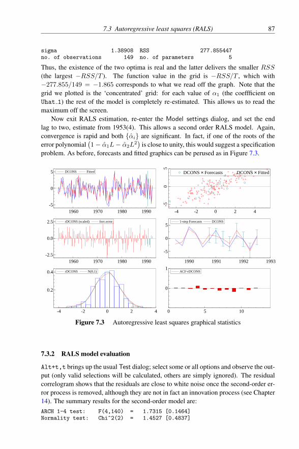
7.3 Autoregressive least squares (RALS) 87
sigma 1.38908 RSS 277.855447no. of observations 149 no. of parameters 5
Thus, the existence of the two optima is real and the latter delivers the smaller RSS(the largest −RSS/T ). The function value in the grid is −RSS/T , which with−277.855/149 = −1.865 corresponds to what we read off the graph. Note that thegrid we plotted is the ‘concentrated’ grid: for each value of α1 (the coeffficient onUhat 1) the rest of the model is completely re-estimated. This allows us to read themaximum off the screen.
Now exit RALS estimation, re-enter the Model settings dialog, and set the endlag to two, estimate from 1953(4). This allows a second order RALS model. Again,convergence is rapid and both αi are significant. In fact, if one of the roots of theerror polynomial
(1− α1L− α2L
2)
is close to unity, this would suggest a specificationproblem. As before, forecasts and fitted graphics can be perused as in Figure 7.3.
DCONS Fitted
1960 1970 1980 1990-5
0
5 DCONS Fitted DCONS × Forecasts DCONS × Fitted
-4 -2 0 2 4
-50
5
DCONS × Forecasts DCONS × Fitted
rDCONS (scaled) forc.error
1960 1970 1980 1990-2.5
0.0
2.5 rDCONS (scaled) forc.error 1-step Forecasts DCONS
1990 1991 1992 1993
-5
0
51-step Forecasts DCONS
rDCONS N(0,1)
-4 -2 0 2 4
0.2
0.4 rDCONS N(0,1) ACF-rDCONS
0 5 10
0
1ACF-rDCONS
Figure 7.3 Autoregressive least squares graphical statistics
7.3.2 RALS model evaluation
Alt+t,t brings up the usual Test dialog; select some or all options and observe the out-put (only valid selections will be calculated, others are simply ignored). The residualcorrelogram shows that the residuals are close to white noise once the second-order er-ror process is removed, although they are not in fact an innovation process (see Chapter14). The summary results for the second-order model are:ARCH 1-4 test: F(4,140) = 1.7315 [0.1464]Normality test: Chi^2(2) = 1.4527 [0.4837]

88 Chapter 7 Tutorial on Estimation Methods
Hetero test: F(6,141) = 0.29588 [0.9380]Hetero-X test: F(9,138) = 0.89207 [0.5342]
The estimated coefficients are (using the Equation format option from Test/Further
results):DCONS = -4.532 - 0.1544*CONS_1 + 0.5154*INC - 0.3586*INC_1 +(SE) (24.9) (0.0817) (0.0365) (0.0687)
0.3743*Uhat_1 + 0.2786*Uhat_2(0.116) (0.0913)
7.4 Non-linear least squaresWe now turn to non-linear least squares (NLS) estimation. This method is shown sep-arately on the Category list under Other models since it applies to any type of data. Italso requires a different method of equation formulation.
PcGive expects us to define a variable called ‘actual’ and a variable called ‘fitted’,expressed in Algebra code. The program can then go ahead to minimize the sum ofsquares (more precisely, PcGive maximizes −RSS/T , see Chapter 17):
min
T∑t=1
ε2t ,
with ε2t defined as:εt = actual− fitted,
and fitted is fitted evaluated at the current parameter values. Parameters are written as&0, &1, . . . , although the numbering does not have to be consecutive. Starting valuesmust always be provided with the code.
We have already considered one method requiring non-linear optimization, namelyRALS. The principles behind NLS are similar except that the flexibility needed in for-mulation to cover a wide class of possible models makes the initial specification morecomplex. We are cheating here initially and have simply set up a linear-least squaresequation.
To facilitate the model formulation, first do OLS of CONS on a Constant, CONS 1,INC and INC 1 over 1953 (2) to 1992 (3) less 8 forecasts. Then use the Non-linear
model format option from Test/Further results) to write the following Algebra code toOxMetrics:actual=CONS;fitted=&0*CONS[-1] + &1 + &2*INC + &3*INC[-1];// starting values:&0=0.9854; &1=5.841; &2=0.5039; &3=-0.4961;
Then bring up the Non-linear model formulation dialog by selecting the Non-linear
modelling Model Class menu and pressing the Formulate button. Copy and paste the
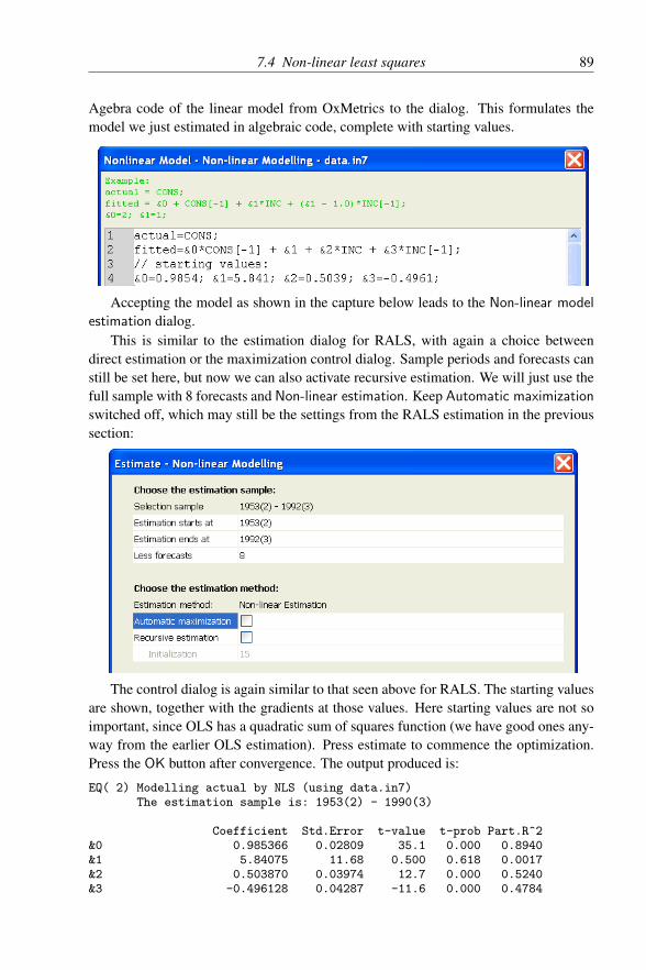
7.4 Non-linear least squares 89
Agebra code of the linear model from OxMetrics to the dialog. This formulates themodel we just estimated in algebraic code, complete with starting values.
Accepting the model as shown in the capture below leads to the Non-linear model
estimation dialog.This is similar to the estimation dialog for RALS, with again a choice between
direct estimation or the maximization control dialog. Sample periods and forecasts canstill be set here, but now we can also activate recursive estimation. We will just use thefull sample with 8 forecasts and Non-linear estimation. Keep Automatic maximization
switched off, which may still be the settings from the RALS estimation in the previoussection:
The control dialog is again similar to that seen above for RALS. The starting valuesare shown, together with the gradients at those values. Here starting values are not soimportant, since OLS has a quadratic sum of squares function (we have good ones any-way from the earlier OLS estimation). Press estimate to commence the optimization.Press the OK button after convergence. The output produced is:
EQ( 2) Modelling actual by NLS (using data.in7)The estimation sample is: 1953(2) - 1990(3)
Coefficient Std.Error t-value t-prob Part.R^2&0 0.985366 0.02809 35.1 0.000 0.8940&1 5.84075 11.68 0.500 0.618 0.0017&2 0.503870 0.03974 12.7 0.000 0.5240&3 -0.496128 0.04287 -11.6 0.000 0.4784

90 Chapter 7 Tutorial on Estimation Methods
sigma 1.48378 RSS 321.435502R^2 0.987924 F(3,146) = 3981 [0.000]**log-likelihood -270.003 DW 1.34no. of observations 150 no. of parameters 4mean(actual) 876.685 var(actual) 177.453
Standard errors based on information matrixBFGS/warm-up using numerical derivatives (eps1=0.0001; eps2=0.005):Strong convergence
1-step (ex post) forecast analysis 1990(4) - 1992(3)Parameter constancy forecast tests:Forecast Chi^2(8) = 7.5050 [0.4833]Chow F(8,146) = 0.90149 [0.5171]
Now we return to undertake a more interesting non-linear estimation, namely mim-icking RALS. Reselect non-linear estimation, which will show the model we had be-fore. This time, restrict the coefficients of the dynamic relation to satisfy the autore-gressive error (that is, COMFAC) restriction for a static regression of CONS on INC:
CONSt = αCONSt−1 + µ+ βINCt − αβINCt−1 + εt,
referring to the previous Algebra code, this imposes &3 = −&0 ∗&2:
actual=CONS;fitted=&0*CONS[-1] + &1 + &2*INC - &0 * &2 * INC[-1];// starting values:&0=0.9854; &1=5.841; &2=0.5039;
Delete the starting value for &3, and accept this formulation; then in the estimation di-alog, check recursive estimation and set the initialization number to 50. OK to move tothe Non-linear estimation dialog. Press Estimate to estimate, and OK to start recursiveestimation.
This is a rather time-consuming computation, which can be interrupted by clickingon the moving icon in the model dialog, to the left of the Formulate button. If youabort, no estimation results will be available.
EQ(4) Modelling actual by NLSThe dataset is: D:\OxMetrics7\data\data.in7The estimation sample is: 1953(2) - 1990(3)
Coefficient Std.Error t-value t-prob Part.R^2&0 0.985760 0.01426 69.1 0.0000 0.9701&1 6.00301 6.077 0.988 0.3248 0.0066&2 0.503653 0.03733 13.5 0.0000 0.5533
sigma 1.47873 RSS 321.436087R^2 0.987865 F(2,147) = 5983 [0.000]**Adj.R^2 0.9877 log-likelihood -270.003no. of observations 150 no. of parameters 3mean(actual) 876.685 se(actual) 13.3658
Standard errors based on information matrix
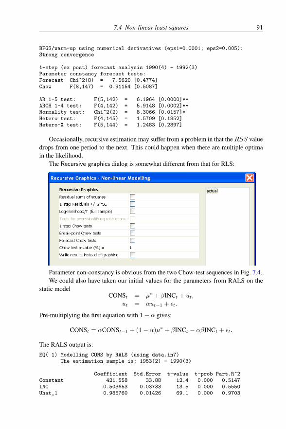
7.4 Non-linear least squares 91
BFGS/warm-up using numerical derivatives (eps1=0.0001; eps2=0.005):Strong convergence
1-step (ex post) forecast analysis 1990(4) - 1992(3)Parameter constancy forecast tests:Forecast Chi^2(8) = 7.5620 [0.4774]Chow F(8,147) = 0.91154 [0.5087]
AR 1-5 test: F(5,142) = 6.1964 [0.0000]**ARCH 1-4 test: F(4,142) = 5.9148 [0.0002]**Normality test: Chi^2(2) = 8.3066 [0.0157]*Hetero test: F(4,145) = 1.5709 [0.1852]Hetero-X test: F(5,144) = 1.2483 [0.2897]
Occasionally, recursive estimation may suffer from a problem in that theRSS valuedrops from one period to the next. This could happen when there are multiple optimain the likelihood.
The Recursive graphics dialog is somewhat different from that for RLS:
Parameter non-constancy is obvious from the two Chow-test sequences in Fig. 7.4.We could also have taken our initial values for the parameters from RALS on the
static modelCONSt = µ∗ + βINCt + ut,
ut = αut−1 + εt.
Pre-multiplying the first equation with 1− α gives:
CONSt = αCONSt−1 + (1− α)µ∗ + βINCt − αβINCt + εt.
The RALS output is:
EQ( 1) Modelling CONS by RALS (using data.in7)The estimation sample is: 1953(2) - 1990(3)
Coefficient Std.Error t-value t-prob Part.R^2Constant 421.558 33.88 12.4 0.000 0.5147INC 0.503653 0.03733 13.5 0.000 0.5550Uhat_1 0.985760 0.01426 69.1 0.000 0.9703

92 Chapter 7 Tutorial on Estimation Methods
RSS
1965 1970 1975 1980 1985 1990
100
200
300RSS Res1Step
1965 1970 1975 1980 1985 1990-5.0
-2.5
0.0
2.5
Res1Step
1up CHOWs 1%
1965 1970 1975 1980 1985 1990
1
2
1up CHOWs 1% Ndn CHOWs 1%
1965 1970 1975 1980 1985 1990
0.5
1.0
Ndn CHOWs 1%
Figure 7.4 Recursive non-linear least squares constancy statistics
sigma 1.47873 RSS 321.436087no. of observations 150 no. of parameters 3
but note the difference in the intercept: in RALS this is µ∗ so is much larger than thevalue for µ = (1−α)µ∗ in the NLS formulation we have adopted. Which form is usedcan substantially affect convergence when α is close to unity. Indeed, if you want tocreate a very badly behaved problem, alter the definition of the intercept to µ/(1 − α)
and plot the grid over a wide range! Great care is needed in formulating the functionto be minimized. Note also the huge time advantage of specifically programmed meth-ods (e.g. RALS) over doing the equivalent in a generic NLS algorithm. Finally, thealternative specification of the constant term ((1−α)µ∗) will lead to different recursivebehaviour: the constant in the former vanishes when α becomes one. If this happens inthe RNLS estimation, this parameter will not be able to get away from 1.
This concludes our tutorial on estimation methods. There are many others to beexplored, and the disk provides several .ALG files for formulating some of the morecommon non-linear models. Further examples are given in Chapter 9.

Chapter 8
Tutorial on Batch Usage
8.1 IntroductionIn this book, the emphasis is very much on interactive use of PcGive. Sometimes, com-mand driven operation can be useful, e.g. as a method of documenting research, or forpreparation of a teaching session. For this purpose, PcGive supports a batch language.As with many other facilities, batch mode operates in cooperation with OxMetrics. Itis in OxMetrics that the batch commands are issued. OxMetrics then decides whetherit can handle the command (e.g. data loading and saving, algebra, database selection).If not, the command is passed on to the active module (use the module command toswitch between e.g. PcGive and STAMP when both are open).
Starting from OxMetrics 5, it is also possible to automatically generate the Oxcode that can rerun the estimations. This Ox code can be run when Ox Professionalor OxMetrics Enterprise (which includes Ox Professional) are available. This allowsfor much more general manipulations of the model inputs or outputs, which can beuseful, e.g., if many models need to be estimated routinely.
8.2 Generating and running Batch codeTo see an example, estimate the familiar model of CONS on a Constant, CONS 1,INC, INC 1, and INFLAT, using the maximum sample with 8 forecasts. Then switch toOxMetrics, and Tools/Batch Editor or use the toolbar button to activate the batch editor.The edit dialog appears, with the current model already formulated in the PcGive batchlanguage, as shown here:
93

94 Chapter 8 Tutorial on Batch Usage
Add some algebra code to create DCONS and DINC, replace CONS and INC in themodel by the first differences, and add the testsummary command, as shown in thecode below:
package("PcGive", "Single-equation");usedata("data.in7");algebra
DCONS = diff(CONS, 1);DINC = diff(INC, 1);
system
Y = DCONS;Z = Constant, CONS_1, DINC, INC_1, INFLAT;
estimate("OLS", 1953, 2, 1992, 3, 8);testsummary;
Press Run to execute the batch file. Once saved to disk, a batch file can also be rundirectly using File/Open, or even by double clicking on the batch file in the Exploreror File Manager. Batch files have the .fl extension, which originally stood for FimlLanguage.
As a last example, use Test/Further Output to write the non-linear model code.Then activate Model/Non-linear modelling to re-estimate the model using NLS. Finally,activate the Batch editor in OxMetrics. Again, an outline batch file has already beenwritten by OxMetrics:

8.3 Generating and running Ox code 95
package("PcGive", "non-linear");usedata("data.in7");nonlinear
actual=DCONS;fitted=&0 + &1*CONS[-1] + &2*DINC + &3*INC[-1] + &4*INFLAT;// starting values:&0=-18.52; &1=-0.1909; &2=0.5067; &3=0.2102; &4=-0.9926;
estimate("NLS", 1953, 2, 1992, 3, 8);
Chapter A1 documents the PcGive batch commands for single equation modelling, andgives a further example.
8.3 Generating and running Ox code
We start by rerunning the Autometrics model selection for the DHSY GUM, at the endof Chapter 6. Then, in OxMetrics, select Model/Ox Batch Code:
The first choice offered is to generate the code for the most recent model, whichis self-evident. The remaining choices are to generate code for all estimated modelsfor any module that was run. Select most recent model, and the code is opened inOxMetrics. If this is the first time you use it in this session, the file will be calledOxBatch 1.ox:
#include <oxstd.h>#import <packages/PcGive/pcgive_ects>
main()// This program requires a licenced version of PcGive Professional.
//--- Ox code for EQ( 2)decl model = new PcGive();
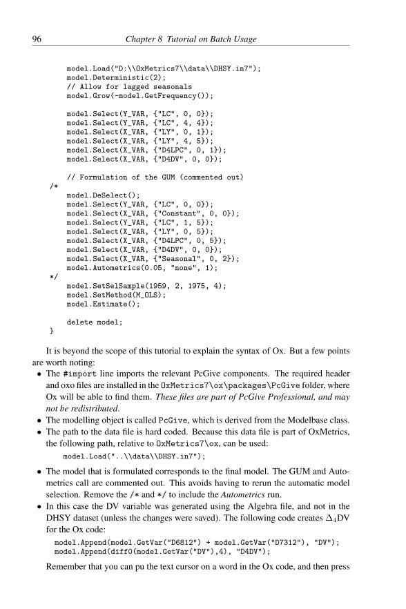
96 Chapter 8 Tutorial on Batch Usage
model.Load("D:\\OxMetrics7\\data\\DHSY.in7");model.Deterministic(2);// Allow for lagged seasonalsmodel.Grow(-model.GetFrequency());
model.Select(Y_VAR, "LC", 0, 0);model.Select(Y_VAR, "LC", 4, 4);model.Select(X_VAR, "LY", 0, 1);model.Select(X_VAR, "LY", 4, 5);model.Select(X_VAR, "D4LPC", 0, 1);model.Select(X_VAR, "D4DV", 0, 0);
// Formulation of the GUM (commented out)/*
model.DeSelect();model.Select(Y_VAR, "LC", 0, 0);model.Select(X_VAR, "Constant", 0, 0);model.Select(Y_VAR, "LC", 1, 5);model.Select(X_VAR, "LY", 0, 5);model.Select(X_VAR, "D4LPC", 0, 5);model.Select(X_VAR, "D4DV", 0, 0);model.Select(X_VAR, "Seasonal", 0, 2);model.Autometrics(0.05, "none", 1);
*/model.SetSelSample(1959, 2, 1975, 4);model.SetMethod(M_OLS);model.Estimate();
delete model;
It is beyond the scope of this tutorial to explain the syntax of Ox. But a few pointsare worth noting:• The #import line imports the relevant PcGive components. The required header
and oxo files are installed in the OxMetrics7\ox\packages\PcGive folder, whereOx will be able to find them. These files are part of PcGive Professional, and maynot be redistributed.
• The modelling object is called PcGive, which is derived from the Modelbase class.• The path to the data file is hard coded. Because this data file is part of OxMetrics,
the following path, relative to OxMetrics7\ox, can be used:model.Load("..\\data\\DHSY.in7");
• The model that is formulated corresponds to the final model. The GUM and Auto-metrics call are commented out. This avoids having to rerun the automatic modelselection. Remove the /* and */ to include the Autometrics run.
• In this case the DV variable was generated using the Algebra file, and not in theDHSY dataset (unless the changes were saved). The following code creates ∆4DVfor the Ox code:model.Append(model.GetVar("D6812") + model.GetVar("D7312"), "DV");model.Append(diff0(model.GetVar("DV"),4), "D4DV");
Remember that you can pu the text cursor on a word in the Ox code, and then press

8.3 Generating and running Ox code 97
F1 for context sensitive help.• For Ox Batch code generation other than the most recent model, the estimated mod-
els are in separate functions, as follows:#include <oxstd.h>#import <packages/PcGive/pcgive_ects>
run_1()
// ...run_2()
// ...main()
run_1();run_2();
The completed program is included in the batch folder as DHSY.ox, and can berun as any other Ox program. More information on Ox programming and running Oxprograms can be found in Doornik and Ooms (2006) and the Ox documentation.

Chapter 9
Non-linear Models
9.1 Introduction
The emphasis of this book is mainly on interactive econometric modelling, primarilyusing OLS, IVE or RALS. However, the non-linear modelling option allows for a wideclass of additional models to be estimated. In the remainder of this chapter we shallfocus on advanced estimation, using the non-linear model option. Both time-series andcross-section examples will be considered. We assume you are familiar with precedingtutorials, especially with the material in Chapters 3 and 7. Note that all models in thischapter can also be estimated using the appropriate packages (discussed in Volume III).This would be more robust, and often gives additional flexibility. However, for teachingpurposes, it is often useful to also implement the model using the non-linear modellingoption.
9.2 Non-linear modelling
Several examples of non-linear least squares estimation were given in Chapter 7. Inparticular, we saw that a linear model can be set up as a non-linear model, but thatdirect estimation by OLS is much more efficient. Estimating RALS and NLS modelsconfronted us with some of the potential problems of estimating non-linear models:1. choosing bad starting values;2. multiple optima;3. for recursive NLS: RSS which is not monotonically increasing with sample size;4. optima which are hard to locate, maybe resulting in failure to converge;5. choosing a ‘difficult’ parametrization (for example, maximizing a concentrated like-
lihood might be easier than the original likelihood).We can add to that:1. programming errors, as we have to program the function ourselves (just try revers-
ing the sign of the ‘loglik’ function);
98

9.3 Maximizing a function 99
2. reaching a region of the parameter space where the function is not defined (such astaking the logarithm of a negative number);
3. failure to compute numerical first derivatives (these are essential for finding an up-ward direction);
4. upon convergence: failure to compute numerical second derivatives (these providestandard errors);
The following four precautions could make the difference between a diverging andconverging estimation:1. scale the parameters, so that they fall between 0.1 and 1 (as a rule of thumb: scale
the explanatory variables to be in the range 0.1–1);2. find good starting values, maybe solving a closely related problem which can be
estimated by OLS;3. use a careful implementation, e.g. take the absolute value (or square) of parameters
that must be positive (such as variances);4. in case of divergence, estimate first with fewer parameters.All these problems have to be taken into account, making non-linear estimation anoption for the advanced user. But it is a powerful feature, and a lot of fun to experimentwith. Many examples are given below.
Sometimes we can show that the log-likelihood is concave, in which case there isonly one maximum. This makes it easier to locate the maximum, and if we find one,we know that it’s the only one. Some things can still go wrong, in the case where thestarting values are too far away from the maximum, or when reaching an area where thefunction is numerically flat. Numerical issues must be considered throughout: e10000
does exist, but our computer cannot handle such a large number.
9.3 Maximizing a functionThe second non-linear estimation method (following NLS) is called ML, which standsfor maximum likelihood. This option maximizes a function of the parameters. Thisdoes not need to be a likelihood function. Consider, for example, minimizing the so-called Rosenbrock function (see Fletcher, 1987):
f(α, β) = 100 ∗(β − α2
)2+ (1− α)
2.
No data are involved. It is easily seen that the minimum is at (1, 1) with functionvalue 0. The contours are rather banana-shaped. To estimate, create a database of justtwo observations in OxMetrics; in that database create a variable with two non-missingvalues. Then in OxMetrics select Other models/Non-linear Modelling and load thetutorial file TutRosen.alg:actual=1; fitted=1;loglik= -100 * (&2 - &1^2)^2 - (1 - &1)^2;&1=0; &2=0;
The variables labelled ‘actual’ and ‘fitted’ are required by PcGive, but serve no otherpurpose here (they are used in the graphic analysis). The ‘loglik’ variable is summed

100 Chapter 9 Non-linear Models
over the sample size, and this sum is minimized. Non-linear modelling requires usto provide starting values, here we choose zero. Accept, select Non-linear estimation
(dialog), accepting the default sample size of two observations. This leads to the Non-
linear Estimation dialog; the top line says ‘Press Estimate to start iterating’, becausethe maximization has not started yet. Push the Estimate button, leading to convergencequickly (the message changes to ‘Strong convergence’). Choosing OK gives the output:EQ( 4) Modelling actual by ML (using Data3)
The estimation sample is: 1 to 2
Coefficient Std.Error t-value t-prob&1 0.999999 0.5000 2.00 0.000&2 0.999999 1.001 0.999 0.000loglik = -9.172049474e-013 for 2 parameters and 2 observations
Standard errors based on numerical second derivativesBFGS/warm-up using numerical derivatives (eps1=0.0001; eps2=0.005):Strong convergence
The output also has a message ‘Warning: invertgen: singular matrix’, which youcan safely ignore here.
9.4 Logit and probit estimationA discrete choice model is one where the dependent variable is discrete, and denotes acategory. In this section we use this type of model to do maximum likelihood estimationin PcGive. Note that these types of models are also directly available in PcGive, seeVolume III (Doornik and Hendry, 2013a). Examples of categorical dependent variablesare:
yi = 0 if household i owns no car,yi = 1 otherwise,
oryi = 0 if individual i travels to work by car,yi = 1 if i travels to work by bike,yi = 2 otherwise.
The first example is a binary choice problem (two categories), the second is multino-mial. Here we restrict ourselves to the former: the dependent variable is a dummy. Witha discrete dependent variable, interest lies in modelling the probabilities of observing acertain outcome. Write
pi = P yi = 1 .
To illustrate this method we use the data from Finney (1947), provided in thefiles Finney.in7 and Finney.bn7. This data set holds 39 observations on the oc-currence of vaso-constriction (the dummy variable, called ‘vaso’) in the skin of thefingers after taking a single deep breath. The dose is measured by the volume ofair inspired (‘volume’) and the average rate of inspiration (‘rate’). Load the dataset into PcGive. A graphical inspection is provided by Figure 9.1. Figure 9.1(a)

9.4 Logit and probit estimation 101
rate × volume × vaso
0.50 0.75 1.00 1.25 1.50 1.75 2.00 2.25 2.50 2.75 3.00 3.25 3.50 3.75
1
2
3
4
11
1
1
11
0
0
000
001
1
1 110
100 0 0
10 10
01 1
0
01 1
1
00 1
rate × volume × vaso
Lrate × Lvolume × vaso
-0.8 -0.6 -0.4 -0.2 0.0 0.2 0.4 0.6 0.8 1.0 1.2
-2
0 111
111
00
000
0 0 11
1 11 010 0 0 0 10 10
01 1
0
01 11
00 1Lrate × Lvolume × vaso
vaso × Lvolume
-0.8 -0.6 -0.4 -0.2 0.0 0.2 0.4 0.6 0.8 1.0 1.20.0
0.5
1.0 vaso × Lvolume
Figure 9.1 Finney’s data
shows a cross-plot of volume and rate by vaso; a 1 indicates the occurrence of vaso-constriction. This graph suggests that response is determined by the product of rateand volume. The next graph uses log(rate) and log(volume). The point inside thecircle appears to be an outlier. The data are taken from the table in Finney (1947),which has a typing error for observation 32. The correct value is (presumably) 0.3instead of 0.03 (0.3 corresponds to the graph in the paper). The straight line in Fig.9.1(c) shows what regressing vaso on log(volume) would lead to; the hand-drawn lineshows a better approach, corresponding to a cumulative distribution function. Apply-ing the straight line (that is, OLS) has several disadvantages here. First, it doesn’tyield proper probabilities, as it is not restricted to lie between 0 and 1 (OLS is calledthe linear probability model: pi = x′iβ). Secondly, the disturbances cannot be nor-mally distributed, as they only take on two values: εi = 1 − pi or εi = 0 − pi.Finally, they are also heteroscedastic: E[εi] = (1 − pi)pi + (0 − pi)(1 − pi) = 0,E[ε2i ] = (1− pi)2pi + (0− pi)2(1− pi) = (1− pi)pi.
A simple solution is to introduce an underlying continuous variable y∗i , which is notobserved. Observed is:
yi =
0 if y∗i < 0,
1 if y∗i ≥ 0.(9.1)
Now we can introduce explanatory variables:
y∗i = x′iβ − εi.
and writepi = P yi = 1 = P x′iβ − εi ≥ 0 = Fε (x′iβ) .

102 Chapter 9 Non-linear Models
Observations with yi = 1 contribute pi to the likelihood, observations with yi = 0
contribute 1− pi:L (β | X) =
∏yi=0
(1− pi)∏yi=1
pi,
and the log-likelihood becomes:
` (β | X) =
N∑i=1
[(1− yi) log (1− pi) + yi log pi] .
The choice of Fε determines the method. Using the logistic distribution:
Fε (z) =ez
1 + ez
leads to logit. Logit has a linear log-odds ratio:
log
(pi
1− pi
)= x′iβ.
The standard normal gives probit. As we can multiply y∗i by any non-zero constantwithout changing the outcome, the scale of these distributions is fixed: the logistic hasvariance π2/3, the standard normal has variance equal to 1. The corresponding Algebracode for our application is:actual = vaso;xbeta = &0 + &1 * Lrate + &2 * Lvolume;fitted = 1 / (1 + exp(-xbeta));loglik = actual * log(fitted) + (1 - actual) * log(1 - fitted);// starting values:&0 = -0.744; &1 = 1.346; &2 = 2.303;
and for probit:actual = vaso;xbeta = &0 + &1 * Lrate + &2 * Lvolume;fitted = probn(xbeta);loglik = actual * log(fitted) + (1-actual) * log(tailn(xbeta));// starting values:&0 = -0.465; &1 = 0.842; &2 = 1.439;
The starting values for both problems were obtained from an OLS regression ofvaso on a constant, Lrate and Lvolume, and then transforming the parameters followingAmemiya (1981) as:
constant restlogit 4 (αOLS − 0.5) 4βOLSprobit 2.5 (αOLS − 0.5) 2.5βOLS
First estimate the binary logit model: load the Finney data set in OxMetrics, inPcGive type Alt+m,l to activate Model/Non-linear modelling. Change database to

9.4 Logit and probit estimation 103
finney.in7, then load TutLogit.alg, accept (if you get the message ‘vaso not found indatabase’ you forgot to change to the finney database) and accept again. In the Non-
linear estimation dialog press Estimate to start estimating, and OK to accept the resultafter convergence. The results are:EQ( 1) Modelling actual by ML (using Finney.in7)
The estimation sample is: 1 - 39
Coefficient Std.Error t-value t-prob&0 -2.87555 1.321 -2.18 0.036&1 4.56176 1.838 2.48 0.018&2 5.17939 1.865 2.78 0.009loglik = -14.61368766 for 3 parameters and 39 observations
Standard errors based on numerical second derivativesBFGS/warm-up using numerical derivatives (eps1=0.0001; eps2=0.005):Strong convergence
vaso plogit liklogit
0 5 10 15 20 25 30 35 40
-2.5
-2.0
-1.5
-1.0
-0.5
0.0
0.5
1.0
liklogit = log(p) if observation has vaso=1 log(1-p) if observation has vaso=0plogit = P(vaso = 1) = p
0.5
vaso plogit liklogit
Figure 9.2 Log-likelihoods, probabilities and outcomes for the logit model
A graphic analysis which will use the variables ‘actual’ and ‘fitted’ as we definedthem is not so interesting here. Better is Figure 9.2. Select Test/Store in database,expand non-linear estimation, click on click on select, and select fitted in the drop-down list. In OxMetrics, rename fitted to plogit. Repeat the same procedure for loglik,renaming it to liklogit. Next, switch to OxMetrics and graph vaso, plogit and liklogit.This graph looks different from 9.2, which is sorted by ‘liklogit’. This is achieved bysorting the whole database by the ‘liklogit’ variable using Algebra; enter:index = trend();_sortallby(liklogit);

104 Chapter 9 Non-linear Models
in the Algebra editor and execute. The index variable allows us to undo the sorting op-eration (but a more simple method is to use the Undo button in OxMetrics). The ‘plogit’variable is pi, whereas ‘liklogit’ is the log-likelihood contribution of observation i: thelog of the probability of being in the observed state. Ideally, we predict a probabilityof one, corresponding to a likelihood of 0. So as we move from left to right, the ‘fit’improves. From the top part of the graph we see that if for pi > 0.5 we would classifythe outcome as a 1, then the misclassifications are on the left.
To see whether the typo in observation 32 matters much, move it to the end of thedatabase through:deselect = (index == 32);_sortallby(deselect);
deselect will be 1 for observation 32 and 0 otherwise, and sorting all variables by des-elect moves number 32 to the bottom. Do a logit model over the sample 1–38: there ishardly any difference at all.
The index variable corresponds to the original observation index, so to restore theoriginal order in the database, execute:_sortallby(index);
and turn to the probit estimation using TutProbit.alg:EQ( 2) Modelling actual by ML (using Finney.in7)
The estimation sample is: 1 - 39Coefficient Std.Error t-value t-prob
&0 -1.50440 0.6375 -2.36 0.024&1 2.51233 0.9365 2.68 0.011&2 2.86200 0.9081 3.15 0.003loglik = -14.64353075 for 3 parameters and 39 observations
Although the coefficients of logit and probit are quite different, this is mainly ow-ing to the choice of scaling parameter. It is more useful to compare probabilities (orderivatives of probabilities with respect to explanatory variables). Sorting the databaseagain, and combining logit and probit results, gives Figure 9.3. Here we see that thedifferences between the results are very small indeed: there is no reason to prefer oneover the other (also see Chambers and Cox, 1967).
As an illustration of the possibilities and drawbacks of PcGive’s ML option wedid a multinomial logit with 4 states (numbered 0,1,2,3), 1700 observations and 24parameters. The probabilities of observation i to be in state j are defined as:
pij =ex
′iβj∑3
j=0 ex′iβj
, j = 0, . . . , 3, with β0 = 0.
The code rearranges this somewhat, to provide a numerically more stable calculation,see MNLOGIT.ALG. On a 90 Mhz Pentium this takes 10 minutes to converge (withstrong convergence tolerance of 0.001), plus nearly 5 minutes to evaluate the variancenumerically. When using the Limited dependent package within PcGive, which em-ploys Newton’s method with analytical first and second derivatives convergence takes4 seconds. Most of the penalty comes out of having to evaluate the algebra code overand over again, rather than being able to use the hard-coded function.

9.5 Tobit estimation 105
vaso plogit liklogit pprobit likprobit
0 5 10 15 20 25 30 35 40
-2.5
-2.0
-1.5
-1.0
-0.5
0.0
0.5
1.0
0.5
vaso plogit liklogit pprobit likprobit
Figure 9.3 Comparison of the probit and logit models
9.5 Tobit estimationIn the standard tobit model (see, for example, Amemiya, 1985, Chapter 10, or Cramer,1986, Chapter 11), the observations on the dependent variable are censored: the positivevalues are observed, but instead of negative values, we see only zeros. The analogue to(9.1) is:
yi =
0 if y∗i ≤ 0,
y∗i if y∗i > 0,
usingy∗i = x′iβ + εi, with εi ∼ IN
(0, σ2
).
Now Py∗i ≤ 0 = P(x′iβ + εi ≤ 0) = 1 − Fε(x′iβ) (Fε is symmetric). The log-likelihood can be seen to consist of a probit part and an OLS part:
` (β | X) =∑yi=0
log (1− Fε (x′iβ)) +∑yi>0
log (fε (yi − x′iβ)) .
Using (13.102):
` (β | X) =∑yi=0
log (1− Fε (x′iβ)) + c+∑yi>0
[log(σ−1
)− 1
2
(yi − x′iβ)2
σ2
]Write Φ for the standard normal cdf:
1− Fε(x′iβ) = 1− Φ (x′iβ/σ) .

106 Chapter 9 Non-linear Models
Using the indicator function I(·) to indicate whether the outcome was observed,`i(β|xi), the likelihood for individual i may be written as:
I (yi = 0) log [1− Φ (x′iβ/σ)] + I (yi > 0)[
12 log
(σ−1
)− 1
2 (yi/σ − x′iβ/σ)2].
It is convenient to scale by σ, writing α = β/σ, so that `i(α|xi) is:
I (yi = 0) log [1− Φ (x′iα)] + I (yi > 0)[
12 log
(σ−1
)− 1
2 (yi/σ − x′iα)2].
The data set is TutTobit.in7, which holds data on expenditure on clothing for 150individuals, with income and age. In algebra code, the likelihood is expressed as (thecode is given in the file TutTobit.alg):actual = expen; // yfitted = &0 + &1 * inc/1000 + &2 * age/10; // x’alphaloglik = (actual <= 0)
? log( max(1.e-20, tailn(fitted)) ) // probit part: log(fabs(&3)) - 0.5 * (actual * fabs(&3) - fitted)^2;
&0=-3.3; &1=1.3; &2=2.3; &3=0.022; // starting valuesfitted = fitted/&3;// undo scaling, fitted is no longer needed
First of all, scaling of the parameters is important, preferably so that they fall be-tween 0.1 and 1. Without that, the numerical derivatives are much more likely to fail.Also use good starting values (here based on OLS). Secondly, &3 is σ−1, and the re-maining parameters estimate α = β/σ. More importantly, we take the absolute valueof &3, reducing the singularity to a small region around 0. Consequently, it is possi-ble to find a negative value for &3; in that case restart at the optimum, but with theabsolute value of &3, which converges immediately. Finally, we don’t allow 1− Fε toget smaller than 10−20. This helps with bad starting values, but should not make anydifference close to the optimum.
The starting values were found from a full-sample OLS estimation:Coefficient Std.Error t-value t-prob Part.R^2
Constant -151.482 48.56 -3.12 0.002 0.0621inc 0.0608239 0.01710 3.56 0.001 0.0792age 10.4385 3.113 3.35 0.001 0.0711
sigma 46.3493 RSS 315793.427R^2 0.23024 F(2,147) = 21.98 [0.000]**
So: &0 = −151.48/46.3439, &1 = (1000 × 0.060824)/46.3439, &2 = (100 ×10.439)/46.3439, &3 = 1/46.3439.
The final results are:EQ( 3) Modelling actual by ML (using TutTobit.in7)
The estimation sample is: 1 to 150
Coefficient Std.Error t-value t-prob&0 -4.78177 1.207 -3.96 0.000&1 1.27797 0.4053 3.15 0.002

9.5 Tobit estimation 107
&2 2.67282 0.7653 3.49 0.001&3 0.0122297 0.001167 10.5 0.000loglik = -374.9303539 for 4 parameters and 150 observations
Figure 9.4 gives a plot of the fitted values from the Tobit model and from OLS inthe upper half, and expenditure in the lower half (both after sorting the database byexpenditure, and for the same expenditure, by income).
OlsFit TobitFit
0 20 40 60 80 100 120 140
-50
0
50
100 OlsFit TobitFit
expen
0 20 40 60 80 100 120 140
100
200
300expen
Figure 9.4 Comparison of fitted values from OLS and Tobit
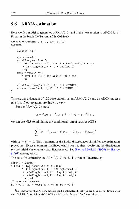
108 Chapter 9 Non-linear Models
9.6 ARMA estimation
Here we fit a model to generated ARMA(2, 2) and in the next section to ARCH data.1
First run the batch file TutArma.fl in OxMetrics:
database("tutarma", 1, 1, 120, 1, 1);algebra
ranseed(-1);
eps = rann();arma22 = year() >= 3
? -1.4 * lag(arma22,1) - .5 * lag(arma22,2) + eps- .2 * lag(eps,1) - .1 * lag(eps,2): 0;
arch = year() >= 3? sqrt(1 + 0.6 * lag(arch,1)^2) * eps: 0;
arma22 = insample(1, 1, 17, 1) ? MISSING;arch = insample(1, 1, 17, 1) ? MISSING;
This creates a database of 120 observations on an ARMA(2, 2) and an ARCH process(the first 17 observations are thrown away).
For the ARMA(2, 2) model
yt = θ0yt−1 + θ1yt−2 + εt + θ2εt−1 + θ3εt−2,
we can use NLS to mimimize the conditional sum of squares (CSS):
T∑t=3
(yt − θ0yt−1 − θ1yt−2 − θ2εt−1 − θ3εt−2)2
with ε1 = ε2 = 0. This treatment of the initial disturbances simplifies the estimationprocedure. Exact maximum likelihood estimation requires specifying the distributionfor the initial observations and disturbances. See Box and Jenkins (1976) or Harvey(1993) among others.The code for estimating the ARMA(2, 2) model is given in TutArma.alg:
actual = arma22;fitted = (lag(actual,2) != MISSING)
? &1*lag(actual,1) + &2*lag(actual,2)+ &3*(lag(actual,1) - lag(fitted,1))+ &4*(lag(actual,2) - lag(fitted,2))
: actual;// starting values:&1 = -1.4; &2 = -0.5; &3 = -0.2; &4 = -0.1;
1Note however, that ARMA models can be estimated directly under Models for time-series
data/ARFIMA models and GARCH models under Models for financial data.
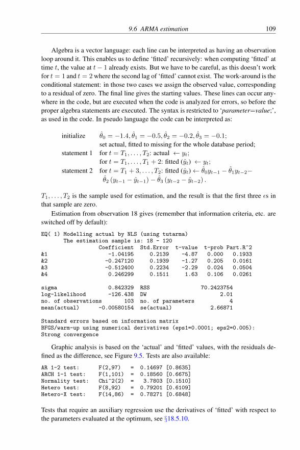
9.6 ARMA estimation 109
Algebra is a vector language: each line can be interpreted as having an observationloop around it. This enables us to define ‘fitted’ recursively: when computing ‘fitted’ attime t, the value at t− 1 already exists. But we have to be careful, as this doesn’t workfor t = 1 and t = 2 where the second lag of ‘fitted’ cannot exist. The work-around is theconditional statement: in those two cases we assign the observed value, correspondingto a residual of zero. The final line gives the starting values. These lines can occur any-where in the code, but are executed when the code is analyzed for errors, so before theproper algebra statements are executed. The syntax is restricted to ‘parameter=value;’,as used in the code. In pseudo language the code can be interpreted as:
initialize θ0 = −1.4, θ1 = −0.5, θ2 = −0.2, θ3 = −0.1;
set actual, fitted to missing for the whole database period;statement 1 for t = T1, . . . , T2: actual ← yt;
for t = T1, . . . , T1 + 2: fitted (yt) ← yt;
statement 2 for t = T1 + 3, . . . , T2: fitted (yt)← θ0yt−1 − θ1yt−2−θ2 (yt−1 − yt−1)− θ3 (yt−2 − yt−2) .
T1, . . . , T2 is the sample used for estimation, and the result is that the first three εs inthat sample are zero.
Estimation from observation 18 gives (remember that information criteria, etc. areswitched off by default):
EQ( 1) Modelling actual by NLS (using tutarma)The estimation sample is: 18 - 120
Coefficient Std.Error t-value t-prob Part.R^2&1 -1.04195 0.2139 -4.87 0.000 0.1933&2 -0.247120 0.1939 -1.27 0.205 0.0161&3 -0.512400 0.2234 -2.29 0.024 0.0504&4 0.246299 0.1511 1.63 0.106 0.0261
sigma 0.842329 RSS 70.2423754log-likelihood -126.438 DW 2.01no. of observations 103 no. of parameters 4mean(actual) -0.00580154 se(actual) 2.66871
Standard errors based on information matrixBFGS/warm-up using numerical derivatives (eps1=0.0001; eps2=0.005):Strong convergence
Graphic analysis is based on the ‘actual’ and ‘fitted’ values, with the residuals de-fined as the difference, see Figure 9.5. Tests are also available:
AR 1-2 test: F(2,97) = 0.14697 [0.8635]ARCH 1-1 test: F(1,101) = 0.18560 [0.6675]Normality test: Chi^2(2) = 3.7803 [0.1510]Hetero test: F(8,92) = 0.79201 [0.6109]Hetero-X test: F(14,86) = 0.78271 [0.6848]
Tests that require an auxiliary regression use the derivatives of ‘fitted’ with respect tothe parameters evaluated at the optimum, see §18.5.10.

110 Chapter 9 Non-linear Models
actual Fitted
20 30 40 50 60 70 80 90 100 110 120-5
0
5 actual Fitted
r:actual (scaled)
20 30 40 50 60 70 80 90 100 110 120
-2
0
2r:actual (scaled)
r:actual N(0,1)
-4 -3.5 -3 -2.5 -2 -1.5 -1 -0.5 0 0.5 1 1.5 2 2.5 3 3.5
0.2
0.4
0.6 Densityr:actual N(0,1)
Figure 9.5 Graphical analysis of ARMA(2,2) model
9.7 ARCH estimation
Specify an ARCH(q) model as:
yt = x′tβ + ut, with ut = σtεt, and σ2t = α0 +
q∑j=1
αju2t−j .
See, for example, Engle (1982) or Bollerslev, Chou, and Kroner (1992). Assuming εt ∼IN(0, 1) gives ut|ut−1 · · ·ut−q ∼ N(0, σ2
t ). So conditional on the past, the model isnormal but heteroscedastic. The log-likelihood for observation t follows from (13.103)
`t (θ|It−1) = c− 12 log
(σ2t
)− 1
2
(yt − x′tβ)2
σ2t
.
Fitting an ARCH(1) model to the generated data, with only a constant in the mean (thatis, the only x is the intercept), is achieved by formulating (see TutArch.alg):
actual = arch;fitted = &0;res = actual - fitted;condv = fabs(&1 + &2 * lag(res,1)^2);loglik = -0.5 * (log(condv) + res^2/condv);&0 = -0.05; &1 = 1.47; &2 = 0.56; // starting values
with β0 = &0, α0 = &1, α1 = &2. The fabs() function takes the absolute value of itsargument. This forces the variance to be positive, and improves the numerical behaviour

9.7 ARCH estimation 111
of the optimization process considerably. The starting values are the coefficients fromthe ARCH test on the residuals from regressing the arch variable on a constant. Theestimated model is, using 8 forecasts:EQ( 3) Modelling actual by ML (using tutarma)
The estimation sample is: 19 - 112
Coefficient Std.Error t-value t-prob&0 -0.0303475 0.1021 -0.297 0.767&1 0.760838 0.1687 4.51 0.000&2 0.543200 0.2150 2.53 0.013loglik = -57.97159729 for 3 parameters and 94 observations
Standard errors based on numerical second derivativesBFGS/warm-up using numerical derivatives (eps1=0.0001; eps2=0.005):Strong convergence
Graphic analysis and some tests are available, but this is not very helpful here be-cause of the definition of ‘actual’ and ‘fitted’: the latter is only a constant. The result isthat ARCH effects are not removed from ‘actual’–‘fitted’, as seen from the test:ARCH 1-1 test: F(1,92) = 17.638 [0.0001]**Normality test: Chi^2(2) = 16.413 [0.0003]**
More useful information is obtained from actual values yt/σt and fitted valuesx′tβ/σt. Re-estimate adding the following to lines at the bottom of the algebra code:actual = arch / sqrt(condv);fitted = &0 / sqrt(condv);
The ARCH test has become insignificant:ARCH 1-1 test: F(1,92) = 0.050393 [0.8229]Normality test: Chi^2(2) = 0.40563 [0.8164]
Some graphical results are in Figure 9.6.As in the ARMA case, it makes a difference how the initial values are treated. In the
ARCH algebra code, the first observations in the estimation use a value determined asactual–fitted when the algebra is run to determine the potential sample period, but leftuntouched during estimation (the value used in this case is 1.4714). It could be fixedby:
// loglik must already existcondv = lag(loglik,1) != MISSING && lag(res,1) != MISSING? fabs(&1 + &2 * lag(res,1)^2) : 1;
This finishes our discussion of non-linear estimation using PcGive. We are confidentthat you can now experiment successfully with your own models.

112 Chapter 9 Non-linear Models
actual Fitted
20 30 40 50 60 70 80 90 100 110 120
-2
0
2 actual Fitted
actual × Forecasts actual × Fitted
-0.018 -0.017 -0.016 -0.015 -0.014 -0.013 -0.012 -0.011 -0.010 -0.009 -0.008 -0.007 -0.006 -0.005 -0.004
-2
0
2 actual × Forecasts actual × Fitted
actual 1-step Forecasts
111 112 113 114 115 116 117 118 119 120 121 122
-1
1 actual 1-step Forecasts
Figure 9.6 Graphical analysis for ARCH model using scaled actual and fitted

Part III
The Econometrics of PcGive


Chapter 10
An Overview
The purpose of Part III is to explain the concepts, models, methods and methodologyembodied in PcGive, and how to interpret its statistical and econometric output. Forcompleteness, we occasionally refer to the module for system modelling which is fullydescribed in Volume II, see Doornik and Hendry (2013c). The aim is to support thelearning of econometrics by using the software at a computer, applying methods todata while learning about those methods. PcGive offers excellent facilities for learn-ing econometrics at all levels from elementary courses, through intermediate stages toadvanced graduate standard. Its ease of use, menu interface and virtual uncrashabilitymake it a straightforward tool even for beginning economists and econometricians.
There are seven chapters on the econometrics of PcGive. First, we describeelementary-level material needed by both economists and econometricians, includingnotions of variation in data, the shape of distributions, measures of association, and timedependence, leading up to dummy variables, collinearity and nonsense regressions. Thethird ‘learning’ chapter is 12, which is at an intermediate level and considers the bulkof the features offered by PcGive. It provides an introductory explanation of econo-metrics, which also serves as a background to many of the features examined in thetutorials. The discussion is intuitive and discursive, and although mathematics is used,this is not at an advanced level. Topics addressed include linear dynamic models andtheir interpretation, multiple regression and instrumental variables, an introduction tomodelling methodology and key econometric concepts, and diagnostic testing. Chapter13 then describes the statistical theory of the normal distribution, of maximum likeli-hood estimation and of least squares, linking that to regression analysis (a distinctiondiscussed shortly).
These chapters establish the main econometric tools, leading in Chapter 14 to anoverview of the approach embodied in PcGive to sustain efficient econometric mod-elling. Chapter 15 considers nine important practical problems. The detailed discussionof the actual statistics reported in PcGive is in Chapters 16–17, relating respectively todata description and single-equation evaluation. As such, they are a reference to be usedas needed, rather than read throughout at a single sitting. Conversely, it is advisable to
115

116 Chapter 10 An Overview
read Chapters 12–14 prior to using PcGive for substantive research. The detailed ta-ble of contents is intended as a quick reference guide for locating explanations aboutany results obtained. References to sections are denoted by chapter.section, for exam-ple, §1.1, §2.4 etc. Equations are denoted by (chapter.number), for example, (12.17).Finally, figures are shown as chapter.number, for example, Figure 13.2.
The philosophy underlying PcGive is that economic time-series data are generatedby a process of immense generality and complexity owing to the interacting behavioursand conflicting objectives of millions of individuals. The outcomes produced by theeconomic mechanism are measured with varying degrees of accuracy, but rarely per-fectly, and sometimes not very well. The combination of the mechanism (the processesof production, transaction and consumption) and the measurement system is called thedata generation process (DGP). The econometrician seeks to model the main features ofthe DGP in a simplified representation based on a small set of observable variables usu-ally related to prior economic theory. Since many important data features are inevitablyassumed absent in any economic theory, empirical models have to be developed inter-actively to characterize the data while being consistent with the theory. For example,a theory model might assume white-noise errors, whereas aggregation and the lack ofa mapping of theory-decision periods to data-observation intervals may mean that theestimated model manifests substantial residual serial correlation (perhaps of a seasonalform). Equally, the ‘deep’ parameters of the theory may correspond to model coeffi-cients which are not empirically constant over time. PcGive is designed to facilitatethe process of model design, reveal problems with potential models, and test models tohighlight their strengths and weaknesses.
Current research suggests that an important component of any modelling exercise isto estimate the most general model that it is reasonable to entertain a priori: see, for ex-ample, Hoover and Perez (1999), and Hendry (2000a, Ch 20). Thus, PcGive facilitatesformulating general linear dynamic models, while still offering protection against thepossibility that the initial generality is in fact too specific to adequately characterize theavailable data. This approach corresponds loosely to a constructive aspect of empiricalmodelling. Both aspects of model construction and testing to destruction are analyzedin Chapter 14.
Many econometrics packages focus on the estimation of economic models of vary-ing degrees of complexity assuming that their qualitative characteristics are known be-forehand, but the numerical values of their parameters need calibration from empiricalevidence. While estimation represents a necessary ingredient in econometrics research,it is far from sufficient for practical empirical modelling. PcGive has been developedto aid the process of discovering ‘good’ models by offering a wide range of evalua-tion tools, some of which are sophisticated estimation methods reoriented to highlightpotential model weaknesses. There is no royal road to developing good models, butsome considerations which have proved helpful in related studies are discussed below,including an analysis of the criteria by which empirical models might be judged. Amore extensive discussion is provided in Hendry (1993), Hendry (2000a) and Hendry(1995a).

117
Just as there is no ‘best’ way to drive a car, but many obviously bad ways (for exam-ple, with your eyes closed), so there are many necessary, but no sufficient, conditionsfor model validity. Delineating these necessary conditions, and analyzing the links be-tween them, the available information and statistics for evaluating model adequacy isthe focus for the discussion in Chapter 14. Here, we begin with data description as thefirst step towards mastering modern econometrics.
Hendry and Nielsen (2007) provide a useful alternative text book, complementingthe material here, and making extensive use of PcGive.

Chapter 11
Learning Elementary EconometricsUsing PcGive
11.1 Introduction
This chapter explains how to use OxMetrics and PcGive to introduce students to econo-metrics, and as a complement to conventional elementary econometrics textbooks.Chapters 14–17 of this manual will be referenced frequently as they have been struc-tured to complement and extend the ideas in the present chapter.
The chapter assumes that the reader has sufficient knowledge to operate PCs run-ning under Windows, and is familiar with OxMetrics/PcGive in terms of its menus,mouse and keyboard. The Tutorials in Part II explain the mechanics of using the pro-gram. On-line, context-sensitive help about the program usage and the econometricsis always available. To load the data used in this chapter, access PCGTUT1.IN7 andPCGTUT1.BN7.
The chapter is also designed to help instructors in teaching econometrics. It isassumed that the instructor has prepared an appropriate data set in an .IN7 + .BN7format: the PCGTUT data set used below is derived from data.in7, data.bn7. Also,it is obvious that the teacher must have explained enough of the usage of PcGive andthe rudiments of Windows so that students can use the program. An overhead computerprojection panel can be linked to a PC for classroom displays. The authors have foundthis to be an admirable and easy vehicle for illustrating econometrics concepts, models,and methods at all levels. As PcGive is essentially uncrashable and models can beformulated in batch files in advance of exercises as required, there is little risk of aserious problem developing — and should the worst happen, it can be turned into asalutory lesson on some of the real difficulties the students will face in undertakingempirical research!
As an initial small data set, we have selected 30 observations on the two variablescons and inc, which are artificial (computer-generated) data interpreted as aggregateconsumers’ expenditure and income in constant prices. First we view the data in the
118
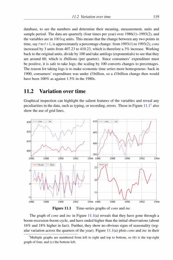
11.2 Variation over time 119
database, to see the numbers and determine their meaning, measurement, units andsample period. The data are quarterly (four times per year) over 1986(1)–1993(2), andthe variables are in 100 log units. This means that the change between any two points intime, say t to t+1, is approximately a percentage change: from 1993(1) to 1993(2), consincreased by 3 units from 407.23 to 410.23, which is therefore a 3% increase. Workingback to the original units, divide by 100 and take antilogs (exponentials) to see that theyare around 60, which is £billions (per quarter). Since consumers’ expenditure mustbe positive, it is safe to take logs; the scaling by 100 converts changes to percentages.The reason for taking logs is to make economic time series more homogenous: back in1900, consumers’ expenditure was under £1billion, so a £1billion change then wouldhave been 100% as against 1.5% in the 1980s.
11.2 Variation over timeGraphical inspection can highlight the salient features of the variables and reveal anypeculiarities in the data, such as typing, or recording, errors. Those in Figure 11.11 alsoshow the use of grid lines.
cons inc
1986 1988 1990 1992 1994
400
410
420
430 cons inc cons inc
1986 1988 1990 1992 1994
395
400
405
410 cons inc
Dcons Dinc
1986 1988 1990 1992 1994
-5
0
5
Dcons Dinc
1986 1988 1990 1992 1994
15
20
25sav sav
Figure 11.1 Time-series graphs of cons and inc
The graph of cons and inc in Figure 11.1(a) reveals that they have gone through aboom-recession-boom cycle, and have ended higher than the initial observations (about16% and 18% higher in fact). Further, they show no obvious signs of seasonality (reg-ular variation across the quarters of the year). Figure 11.1(a) plots cons and inc in their
1Multiple graphs are numbered from left to right and top to bottom, so (b) is the top-rightgraph of four, and (c) the bottom left.

120 Chapter 11 Learning Elementary Econometrics Using PcGive
original units, whereas Figure 11.1(b) matches them by means and ranges to maximizetheir apparent visual closeness: this helps reveal whether or not the two series move inthe general way.
Now copy cons to a new variable, then revise the observation in 1987(1) from401.41 to 301.41; it can be hard to notice this error in the database – and would bevery hard amongst 500 data points – but a glance at its graph makes such an error clear.Remember to change the mistake back if you did not use a copy of cons.
Time-series graphs of the differences of, or changes in, each variable highlight theperiods of positive and negative growth and show any synchrony between the series.Let ∆cons and ∆inc denote the changes from quarter to quarter (the Greek symbol∆ is often used in that sense in econometrics). Figure 11.1(c) shows that changes inthese two series, unmatched, are clearly very close. Finally, Figure 11.1(d) plots thedifference inc–cons which is called sav (actually, this is 100 times the savings ratio).
395 400 405 410
2.5
5.0
7.5cons
410 415 420 425 430 435
2
4
6inc
-4 -2 0 2 4 6
2
4
6Dcons
-5 0 5 10
2.5
5.0
7.5 Dinc
Figure 11.2 Histograms of cons and inc
11.3 Variation across a variable
It is also useful to summarize data in terms of their distributional shape and low-ordermoments, and we illustrate this feature using the OxMetrics graphics. Click the graph-
ics option and select cons, inc and their changes, then select Distribution/Frequencies
as graph type. This leads to the outcomes in Figure 11.2(a)–(d). Here, there are too fewdata points to make the shape of the distributions very clear other than near symmetry,but we comment on several aspects in the next section.
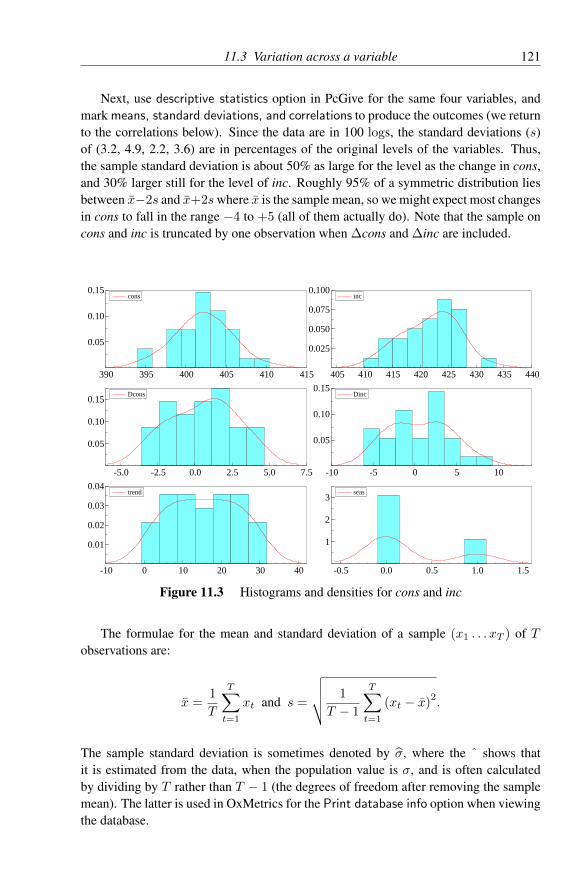
11.3 Variation across a variable 121
Next, use descriptive statistics option in PcGive for the same four variables, andmark means, standard deviations, and correlations to produce the outcomes (we returnto the correlations below). Since the data are in 100 logs, the standard deviations (s)of (3.2, 4.9, 2.2, 3.6) are in percentages of the original levels of the variables. Thus,the sample standard deviation is about 50% as large for the level as the change in cons,and 30% larger still for the level of inc. Roughly 95% of a symmetric distribution liesbetween x−2s and x+2swhere x is the sample mean, so we might expect most changesin cons to fall in the range −4 to +5 (all of them actually do). Note that the sample oncons and inc is truncated by one observation when ∆cons and ∆inc are included.
cons
390 395 400 405 410 415
0.05
0.10
0.15cons inc
405 410 415 420 425 430 435 440
0.025
0.050
0.075
0.100inc
Dcons
-5.0 -2.5 0.0 2.5 5.0 7.5
0.05
0.10
0.15Dcons Dinc
-10 -5 0 5 10
0.05
0.10
0.15Dinc
trend
-10 0 10 20 30 40
0.01
0.02
0.03
0.04trend seas
-0.5 0.0 0.5 1.0 1.5
1
2
3seas
Figure 11.3 Histograms and densities for cons and inc
The formulae for the mean and standard deviation of a sample (x1 . . . xT ) of Tobservations are:
x =1
T
T∑t=1
xt and s =
√√√√ 1
T − 1
T∑t=1
(xt − x)2.
The sample standard deviation is sometimes denoted by σ, where the ˆ shows thatit is estimated from the data, when the population value is σ, and is often calculatedby dividing by T rather than T − 1 (the degrees of freedom after removing the samplemean). The latter is used in OxMetrics for the Print database info option when viewingthe database.

122 Chapter 11 Learning Elementary Econometrics Using PcGive
11.4 Populations, samples and shapes of distributions
Next, we relate the sample of data that was observed to the population of possibleoutcomes that might have occurred. We can use interpolated data densities to show theunderlying shapes of the distributions (the estimated density and histogram graph type).As Figure 11.3 reveals, cons is unimodal and close to a normal distribution whereas∆cons (the first difference) is nearer to a uniform distribution; inc and ∆inc are moreerratic – and the latter is nearly bimodal. The figure also shows other densities: theseasonal (called seas) is clearly bimodal, with one bump much larger than the other,and the trend is nearly uniform (can you explain these last two outcomes?).2
cons × normal
397.5 400.0 402.5 405.0 407.5
395
400
405
410 cons × normal inc × normal
412.5 415.0 417.5 420.0 422.5 425.0 427.5 430.0
415
420
425
430
435inc × normal
Dcons × normal
-2 0 2 4
-2.5
0.0
2.5
5.0Dcons × normal Dinc × normal
-5.0 -2.5 0.0 2.5 5.0 7.5
-5
0
5
Dinc × normal
Figure 11.4 QQ plots for cons and inc
The (cumulative) distribution function is one of the most basic concepts in prob-ability, as it contains all the information about the probability behaviour of a randomvariable. Plot these for the same six variables (note that the normal is plotted auto-matically as well) and compare: the OxMetrics book discusses creating densities anddistributions for the standard statistical distributions. So-called QQ plots offer a pictureof the closeness to normality of a variable: those in Figure 11.4 show the transformedcumulative distribution of the sample data with that for the normal (which is a straightline). There are departures in the tails, but otherwise little evidence against normality.
2To create these indicator variables in the database, use the algebra code: one = 1; trend =trend(); seas = season();. Note that they are automatically provided when estimating a model.
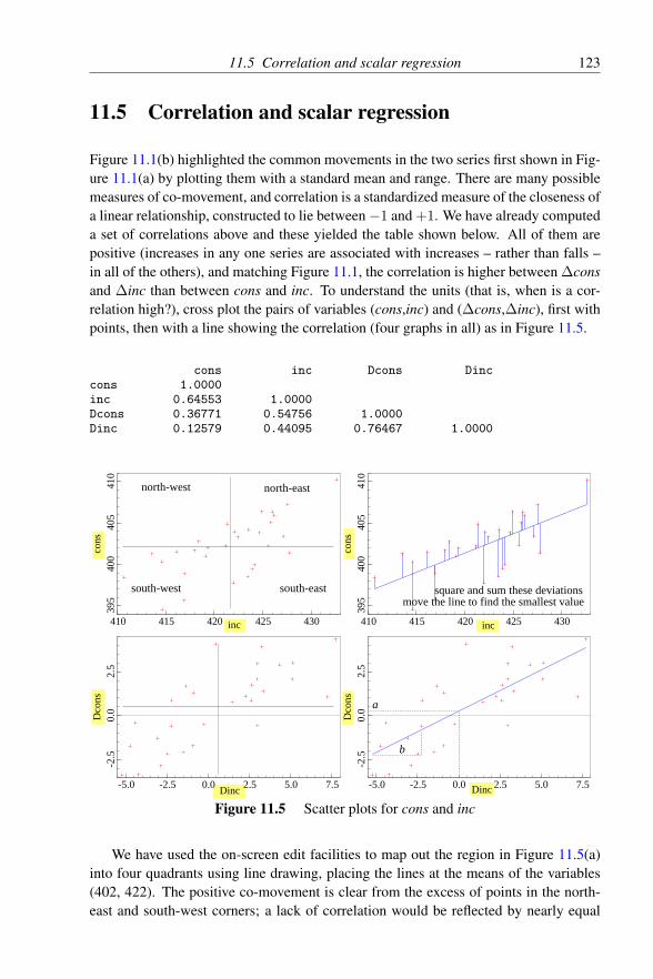
11.5 Correlation and scalar regression 123
11.5 Correlation and scalar regression
Figure 11.1(b) highlighted the common movements in the two series first shown in Fig-ure 11.1(a) by plotting them with a standard mean and range. There are many possiblemeasures of co-movement, and correlation is a standardized measure of the closeness ofa linear relationship, constructed to lie between−1 and +1. We have already computeda set of correlations above and these yielded the table shown below. All of them arepositive (increases in any one series are associated with increases – rather than falls –in all of the others), and matching Figure 11.1, the correlation is higher between ∆consand ∆inc than between cons and inc. To understand the units (that is, when is a cor-relation high?), cross plot the pairs of variables (cons,inc) and (∆cons,∆inc), first withpoints, then with a line showing the correlation (four graphs in all) as in Figure 11.5.
cons inc Dcons Dinccons 1.0000inc 0.64553 1.0000Dcons 0.36771 0.54756 1.0000Dinc 0.12579 0.44095 0.76467 1.0000
410 415 420 425 430
395
400
405
410
inc
cons
north-west north-east
south-west south-east
410 415 420 425 430
395
400
405
410
inc
cons
square and sum these deviationsmove the line to find the smallest value
-5.0 -2.5 0.0 2.5 5.0 7.5
-2.5
0.0
2.5
Dinc
Dco
ns
-5.0 -2.5 0.0 2.5 5.0 7.5
-2.5
0.0
2.5
Dinc
Dco
ns
b
a
Figure 11.5 Scatter plots for cons and inc
We have used the on-screen edit facilities to map out the region in Figure 11.5(a)into four quadrants using line drawing, placing the lines at the means of the variables(402, 422). The positive co-movement is clear from the excess of points in the north-east and south-west corners; a lack of correlation would be reflected by nearly equal
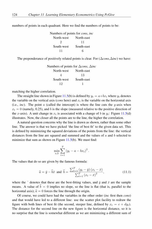
124 Chapter 11 Learning Elementary Econometrics Using PcGive
numbers of points in each quadrant. Here we find the numbers of points to be:
Numbers of points for cons, incNorth-west
2
North-east11
South-west11
South-east6
The preponderance of positively related points is clear. For (∆cons,∆inc) we have:
Numbers of points for ∆cons, ∆incNorth-west
4
North-east13
South-west12
South-east1
matching the higher correlation.The straight line shown in Figure 11.5(b) is defined by yt = a+bxt where yt denotes
the variable on the vertical axis (cons here) and xt is the variable on the horizontal axis(i.e., inc). The point a (called the intercept) is where the line cuts the y-axis whenxt = 0 (namely, 0.25), and b is the slope (measured relative to the positive direction ofthe x-axis). A unit change in xt is associated with a change of b in yt: Figure 11.5(d)illustrates. Now, the closer all the points are to the line, the higher the correlation.
A natural question concerns why the line is drawn as shown, rather than some otherline. The answer is that we have picked ‘the line of best fit’ to the given data set. Thisis defined by minimizing the squared deviations of the points from the line: the verticaldistances from the line are squared and summed and the values of a and b selected tominimize that sum as shown on Figure 11.5(b). We must find:
mina,b
T∑t=1
(yt − a− bxt)2.
The values that do so are given by the famous formula:
a = y − bx and b =
∑Tt=1 (yt − y) (xt − x)∑T
t=1 (xt − x)2
, (11.1)
where the ˆ denotes that these are the best-fitting values, and y and x are the samplemeans. A value of b = 0 implies no slope, so the line is flat (that is, parallel to thehorizontal axis); a = 0 forces the line through the origin.
Of course, we could have had the variables in the other order (inc first then cons)and that would have led to a different line: use the scatter plot facility to redraw thefigure with both lines of best fit (the second, steeper line, defined by xt = c + dyt).The distance for the second line on the new figure is the horizontal distance, so it isno surprise that the line is somewhat different as we are minimizing a different sum of

11.5 Correlation and scalar regression 125
squared deviations. Indeed:
c = x− dy and d =
∑Tt=1 (xt − x) (yt − y)∑T
t=1 (yt − y)2
. (11.2)
These two possible lines are closely related to the correlation coefficient, which wedenote by r:
r =
∑Tt=1 (xt − x) (yt − y)√∑T
t=1 (xt − x)2∑T
t=1 (yt − y)2. (11.3)
From (11.1) and (11.2), it can be seen that bd = r2. When r = 1 (or −1) the two linescoincide; when r = 0, they are both parallel to their respective axes, so are at rightangles to each other.
Using PcGive, it is easy to calculate the outcomes from fitting the line shown in thegraph. The procedure is often called regression (somewhat loosely as we will see later).Access the Cross-section regression option and select cons as dependent (yt) and inc asexplanatory (xt), leading to:
EQ( 1) Modelling cons by OLS (using PcgTut1.in7)The estimation sample is: 1986 (1) to 1993 (2)
Coefficient Std.Error t-value t-prob Part.R^2Constant 206.006 40.36 5.10 0.000 0.4820inc 0.465140 0.09571 4.86 0.000 0.4576
sigma 2.58918 RSS 187.707974R^2 0.457558 F(1,28) = 23.62 [0.000]**log-likelihood -27.5054 DW 0.317no. of observations 30 no. of parameters 2mean(cons) 402.148 var(cons) 11.5347
The important information for the present is that the intercept (called Constant) is a =
206 and the slope b = 0.465. The numbers denoted Std.Error are the standard errors,or the standard deviations, of the estimated coefficients of the intercept and slope, so±2× 0.09571 is an approximate 95% confidence interval around the central value b =
0.4651. The symbol Rˆ2 is just the square of r = 0.676 and sigma (for σ) denotes thestandard deviation of the residuals about the line, where the residuals are:
ut = yt − a− bxt so σ =
√√√√ 1
T − 2
T∑t=1
u2t . (11.4)
Thus, the line is picked to yield the smallest value of σ. RSS denotes the residual sumof squares, namely:
RSS =
T∑t=1
u2t .
The symbol F is a test of whether the correlation is zero, and ∗∗ denotes that it isdefinitely not (the probability is essentially zero of getting the value 23.62 for F whenr = 0 – shown as [0.0000]).
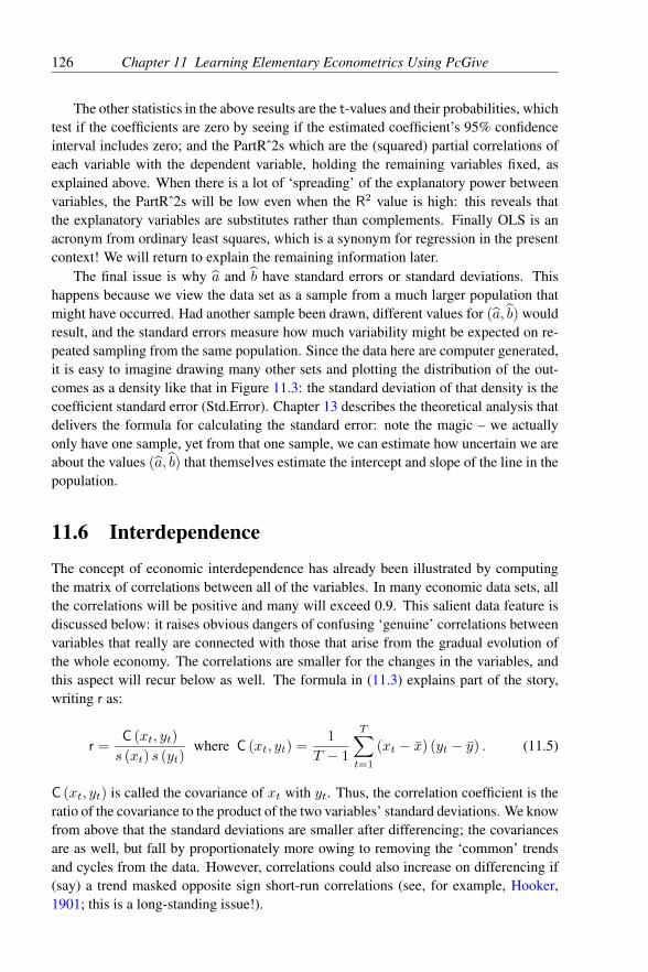
126 Chapter 11 Learning Elementary Econometrics Using PcGive
The other statistics in the above results are the t-values and their probabilities, whichtest if the coefficients are zero by seeing if the estimated coefficient’s 95% confidenceinterval includes zero; and the PartRˆ2s which are the (squared) partial correlations ofeach variable with the dependent variable, holding the remaining variables fixed, asexplained above. When there is a lot of ‘spreading’ of the explanatory power betweenvariables, the PartRˆ2s will be low even when the R2 value is high: this reveals thatthe explanatory variables are substitutes rather than complements. Finally OLS is anacronym from ordinary least squares, which is a synonym for regression in the presentcontext! We will return to explain the remaining information later.
The final issue is why a and b have standard errors or standard deviations. Thishappens because we view the data set as a sample from a much larger population thatmight have occurred. Had another sample been drawn, different values for (a, b) wouldresult, and the standard errors measure how much variability might be expected on re-peated sampling from the same population. Since the data here are computer generated,it is easy to imagine drawing many other sets and plotting the distribution of the out-comes as a density like that in Figure 11.3: the standard deviation of that density is thecoefficient standard error (Std.Error). Chapter 13 describes the theoretical analysis thatdelivers the formula for calculating the standard error: note the magic – we actuallyonly have one sample, yet from that one sample, we can estimate how uncertain we areabout the values (a, b) that themselves estimate the intercept and slope of the line in thepopulation.
11.6 Interdependence
The concept of economic interdependence has already been illustrated by computingthe matrix of correlations between all of the variables. In many economic data sets, allthe correlations will be positive and many will exceed 0.9. This salient data feature isdiscussed below: it raises obvious dangers of confusing ‘genuine’ correlations betweenvariables that really are connected with those that arise from the gradual evolution ofthe whole economy. The correlations are smaller for the changes in the variables, andthis aspect will recur below as well. The formula in (11.3) explains part of the story,writing r as:
r =C (xt, yt)
s (xt) s (yt)where C (xt, yt) =
1
T − 1
T∑t=1
(xt − x) (yt − y) . (11.5)
C (xt, yt) is called the covariance of xt with yt. Thus, the correlation coefficient is theratio of the covariance to the product of the two variables’ standard deviations. We knowfrom above that the standard deviations are smaller after differencing; the covariancesare as well, but fall by proportionately more owing to removing the ‘common’ trendsand cycles from the data. However, correlations could also increase on differencing if(say) a trend masked opposite sign short-run correlations (see, for example, Hooker,1901; this is a long-standing issue!).

11.7 Time dependence 127
11.7 Time dependence
Correlations (or dependencies) between successive values of the same variable oftenoccur in economic time series. These are called serial (or auto) correlations. FromFigure 11.1, when cons was high, the next value was also high, and when low, so wasthe next value. In general, we denote the current value of a variable by yt and itsprevious (or lagged) value by yt−1. The difference is then ∆yt = yt − yt−1.
395.0 397.5 400.0 402.5 405.0 407.5
395
400
405
410
const−1
cons
t
412.5 415.0 417.5 420.0 422.5 425.0 427.5
415
420
425
430
435
inct−1
inc t
-3 -2 -1 0 1 2 3 4
-2.5
0.0
2.5
∆const−1
∆con
s t
-5.0 -2.5 0.0 2.5 5.0 7.5
-50
5
∆inct−1
∆inc
t
Figure 11.6 Lagged scatter plots for cons and inc
Figure 11.1 also revealed that ∆cons jumped around considerably: high values werenot followed by other high values very often. By simple algebra, when ∆yt is indepen-dent over time (so is not related to ∆yt−1), then yt ' yt−1 and hence yt is seriallycorrelated.
A useful way to see time dependence is to cross plot yt against yt−1, and ∆ytagainst ∆yt−1 with a least-squares line (as in Figure 11.6). You may need to create thelagged values using the calculator (shown as cons1 etc.). It is clear that cons and incare both highly correlated with their own lagged values (Figure 11.6(a) and 11.6(b)),whereas ∆cons and ∆inc are nearly unrelated (horizontal regression lines).
This idea can be generalized to two-period relations, namely the correlation of ytwith yt−2. To summarize all such correlations at once, we plot a correlogram (or auto-correlation function, ACF) with the correlations rj = corr(yt, yt−j) on the vertical axisand j on the horizontal, illustrated for four terms (j = 1, . . . , 4) in Figure 11.7. Thisidea relates back to the salient feature of serial dependence of the time-series graphsof the variables in Figure 11.1, and provides a quantitative measurement of that aspect.Here, the correlograms for cons and inc have several large positive terms, whereas those

128 Chapter 11 Learning Elementary Econometrics Using PcGive
for ∆cons and ∆inc are nearly zero at all lags. The values of r1 reflect the slopes ofthe plots in Figure 11.6. The horizontal dashed lines are rj ± 2SE for the estimatedautocorrelations, assuming the population value is zero: thus r1 is unlikely to be zerofor cons and inc.
ACF-cons
0 1 2 3 4 5 6
-0.5
0.0
0.5
1.0ACF-cons ACF-inc
0 1 2 3 4 5 6
0.25
0.50
0.75
1.00ACF-inc
ACF-Dcons
0 1 2 3 4 5 6
-0.5
0.0
0.5
1.0ACF-Dcons ACF-Dinc
0 1 2 3 4 5 6
-0.5
0.0
0.5
1.0ACF-Dinc
Figure 11.7 Sample ACF for cons and inc
We are in fact implicitly using regression, and can compute the slope coefficientfor yt on yt−1, called a first-order autoregression (‘regression on itself’), using thatmethod. Select the Single-equation dynamic modelling option for cons, choose onelag, and accept to obtain (the last three lines are omitted):
EQ( 2) Modelling cons by OLS (using PcgTut1.in7)The estimation sample is: 1986 (2) to 1993 (2)
Coefficient Std.Error t-value t-prob Part.R^2cons_1 0.764263 0.1282 5.96 0.000 0.5684Constant 95.2765 51.51 1.85 0.075 0.1125
sigma 2.13872 RSS 123.501614R^2 0.568417 F(1,27) = 35.56 [0.000]**
By now the statistics should be becoming more familiar: the intercept is 95.28 and theslope (i.e., the autoregressive coefficient) is 0.7643 which is approximately equal to theautocorrelation of r1 = 0.754 (i.e., the square root of R2). The value of r1 is, therefore,just that of the correlation coefficient calculated as in (11.3) for cons and cons1, andshows the slope of the regression line in the graph of that variable against its laggedvalue. Try to prove these connections for a first-order autoregression.
Returning to the correlogram rj, a new idea occurs: we know corr (yt, yt−1) and

11.8 Dummy variables 129
corr (yt, yt−2) but part of each of these may be owing to the other – can we sort outthe ‘net’ contributions of the one and two period lags? One notion might be to use theresiduals from the first-order autoregression and correlate these with yt−2; this approachgets close, but on reflection, you can probably see that it takes out too much of yt−1 atthe first step (that is, it also takes out the bit of yt−2 in yt−1). We believe the easiestway to understand the notion is to fit the regression of yt on both yt−1 and yt−2 whichis simple to perform in PcGive. Select the Single-equation dynamic modelling optionfor cons again but this time choose two lags and accept to obtain:
EQ( 3) Modelling cons by OLS (using PcgTut1.in7)The estimation sample is: 1986 (3) to 1993 (2)
Coefficient Std.Error t-value t-prob Part.R^2cons_1 0.747621 0.2129 3.51 0.002 0.3304cons_2 -0.0295917 0.2015 -0.147 0.884 0.0009Constant 113.896 62.50 1.82 0.080 0.1173
sigma 2.20625 RSS 121.688116R^2 0.490759 F(2,25) = 12.05 [0.000]**
The first slope coefficient is almost the same as that obtained when yt−1 alone was used,and consistent with that, the second is close to zero. We learn that most of corr (yt, yt−2)
is due to the effect of yt−1, and no ‘net’ 2-period lag operates. This is important in un-derstanding the pattern we observed in the correlogram. The generalization we havedeveloped is called the partial autocorrelation. The first slope coefficient shows thechange in yt from a change in yt−1 when yt−2 does not change: the second slope coef-ficient shows the change in yt from a change in yt−2 when yt−1 does not change. Eachshows the net effect of its variable – together they show the total effect. A great ad-vantage of regression methods is this ease of generalization to any number of variables,where each coefficient measures the effects on the dependent variable of changing thatexplanatory variable when all other variables are held fixed. Chapter 13 describes thenecessary algebra.
11.8 Dummy variables
Dummy variables are artificial creations with their non-zero values determined by us,rather than by nature. They are often called indicator variables as they indicate thepresence of some state. We have already met three, namely the Constant, Trend andSeasonal (where the first does not vary, so indicates the constant state!). The Seasonalindicator variable (for non-annual data) is automatically created by PcGive to be unityin the first period of the year and zero elsewhere. PcGive only needs one seasonal fromwhich the remaining seasonals for other periods are created by lagging: Seasonal 2 isSeasonal two periods lagged, and so has a unity in the third period of each year. Usingthe calculator or algebra, other dummies are easily created in a variety of forms forimpulse effects (a ‘blip’ which is zero except for perhaps a couple of quarters where itis unity, often called a zero-one dummy); and step changes where the dummy is zero

130 Chapter 11 Learning Elementary Econometrics Using PcGive
until a certain date and unity thereafter. Note that the scale of measurement of a dummyis ordinal (‘on’ differs from ‘off’) in that the ‘on’ effect can bear any relation to the ‘off’.It is dangerous to create a dummy which takes three or more values (for example, somezeros, some unities and some twos) unless you are certain that the effect of the third istwice that of the second. However, we will do just that – for a specific purpose. Use thealgebra to create the variable qrtr=period(); and using scatter plot, graph cons, incand qrtr (after Next choose graph, select two series by a third). The figure will showthe points as 1,2,3,4 depending on the quarter of the year, so the relation of cons to incin each quarter can be viewed. For the present data, the picture in Figure 11.8a is nottoo informative, but see Davidson, Hendry, Srba, and Yeo (1978) for a clearer example.
Next, graph cons and the trend over time, match for mean and range; then also crossplot them with the points joined; finally cross-plot them again, and insert a regressionline as in Figure 11.8. The first cross plot (Figure 11.8c) shows precisely the time-series plot of cons; whereas the second cross plot shows the best-fitting trend line,which clearly differs from that obtained by just matching means and ranges (which isalmost inevitably too steep).
Finally, note that a complete set of indicator variables is never needed (for example,a dummy for ‘on’ and a second dummy for ‘off’) and is said to be perfectly collinear.Try to compute a regression of cons on the quarterly seasonal with three lags: contrastthe outcome with what happens when you use only two lags, where a constant is alwaysincluded.
410 415 420 425 430
395
400
405
410
inc
cons
12
34
12
3
41
234
123
4
1
2
3 4
12
341
23
41
2cons trend
1985 1990
395
400
405
410 cons trend
0 5 10 15 20 25 30
395
400
405
410
trend
cons
0 5 10 15 20 25 30
395
400
405
410
trend
cons
Figure 11.8 Relating time series and cross-plots using dummy variables

11.9 Sample variability 131
11.9 Sample variability
Histograms and densities showed the data variability; this section focuses on the vari-ability in the sample statistics. Use the zoom sample check box to cross plot consagainst inc with a single regression line for the first half of the data only (to 1989(3)),then for the second half only. Now redo the cross plot for the whole sample periodtwice, but first fit two sequential lines then two recursive lines. The outcome is shownin Figure 11.9. The regression lines for the two subsamples clearly differ in slope andintercept, as Figure 11.9c makes clear (compute these numerically using the Single-
equation dynamic modelling option to check). Nevertheless, as Figure 11.9d reveals,the first sample line is close to that obtained for the whole period.
Try fitting a number of sequential lines (four, for example) and consider the out-come, perhaps using several trend lines, to show growth-rate changes. This exerciseshould clarify the need to report coefficient standard errors.
415.0 417.5 420.0 422.5 425.0 427.5
395
398
401
404
407
inc
cons
410 415 420 425 430
400
403
406
409
412
inc
cons
410 415 420 425 430
395
400
405
410
inc
cons
410 415 420 425 430
395
400
405
410
inc
cons
Figure 11.9 Changing regression lines
11.10 Collinearity
Perfect linear dependence was shown in §11.8 above; this item relates to ‘near lineardependence’ between regressors – a more rigorous analysis is provided in §15.1. Weintroduced multiple regression above using the example of partial autocorrelation, andnow use a finite distributed lag to show the effects of adding xt−1 to the regression ofyt on xt. This is called a distributed lag model because the lag coefficients on x show

132 Chapter 11 Learning Elementary Econometrics Using PcGive
the distribution of the response of y over time (and when they are all positive, the coef-ficients can be normalized to add to unity, and hence are like a probability distribution).When xt is highly autoregressive, a large increase in coefficient uncertainty usually re-sults as the ‘explanation’ of yt gets spread between xt and xt−1 rather than concentratedon the former. Choose cons for yt and inc for xt and use the Single-equation dynamic
modelling option with one lag on inc to produce:
EQ( 4) Modelling cons by OLS (using PcgTut1.in7)The estimation sample is: 1986 (2) to 1993 (2)
Coefficient Std.Error t-value t-prob Part.R^2Constant 202.060 44.39 4.55 0.000 0.4435inc 0.301206 0.1352 2.23 0.035 0.1602inc_1 0.173896 0.1432 1.21 0.235 0.0537
sigma 2.46474 RSS 157.948781R^2 0.448039 F(2,26) = 10.55 [0.000]**
The standard error of the coefficient of xt has increased by over 40% from the simpleregression: this effect is often called collinearity, and is viewed as deriving from thehigh correlation between xt and xt−1 when both are used to explain yt.
At a somewhat more advanced level, instead of xt−1, add ∆xt to the regression ofyt on xt and consider the new output:
EQ( 5) Modelling cons by OLS (using PcgTut1.in7)The estimation sample is: 1986 (2) to 1993 (2)
Coefficient Std.Error t-value t-prob Part.R^2Constant 202.060 44.39 4.55 0.000 0.4435inc 0.475102 0.1053 4.51 0.000 0.4392Dinc -0.173896 0.1432 -1.21 0.235 0.0537
sigma 2.46474 RSS 157.948781R^2 0.448039 F(2,26) = 10.55 [0.000]**
A glance establishes that all the regression statistics R2, s, F etc. are identical to the ear-lier distributed lag estimates, and apart from the sign, so is the coefficient and standarderror of ∆inc. Only the coefficient and standard error of inc have altered (the formerto the sum of the coefficients in the distributed lag), both close to those found in thesimple regression of cons on inc. In fact, these last two models are actually equivalent,as is easily seen algebraically:
d1xt + d2xt−1 ≡ (d1 + d2)xt − d2 (xt − xt−1) .
The differences in the standard errors between the two equivalent parametrizationsare owing to the relatively low correlation between xt and ∆xt, which must happenwhen xt and xt−1 are highly correlated. This highlights the advantages of orthogonalparametrizations (ones where explanatory variables are not correlated) where these arefeasible.
An alternative way to create collinearity is to add yt−1 to the regression of yt on xt;again use cons and inc to obtain:

11.11 Nonsense regressions 133
EQ( 6) Modelling cons by OLS (using PcgTut1.in7)The estimation sample is: 1986 (2) to 1993 (2)
Coefficient Std.Error t-value t-prob Part.R^2cons_1 0.634611 0.09665 6.57 0.000 0.6238Constant 16.5568 40.59 0.408 0.687 0.0064inc 0.310060 0.06184 5.01 0.000 0.4916
sigma 1.55403 RSS 62.7904156R^2 0.780575 F(2,26) = 46.25 [0.000]**
This time, despite the correlation between the explanatory variables, there is almost noincrease in the standard error of the coefficient of inc (in fact cons lagged and inc areonly correlated 0.27). Notice the counterbalancing effects of the improvement in fitfrom the added variable against its interrelation with the previously-included variable.Contrast the outcomes in this section with those found from (say) regressing ∆yt on∆xt (or that with ∆yt−1 added).
11.11 Nonsense regressions
Even at an elementary level, a critical appreciation of econometric evidence is essential,especially for time-series econometrics. The issue of invalidly ‘inferring causes fromcorrelations’ must be discussed: high (low) correlations do not by themselves confirm(refute) causal links. Rather, theory-models with well-defined causality links can betested from data by checking on the presence and/or absence of certain correlationspredicted by those models. Models which fail must be rejected, or at a minimum re-vised; models that are not rejected are consistent with the theory. This is a deductiveexercise. Rigorously-tested, yet acceptable, models are then used in later analyticalwork, but causes are never inferred from correlations.
The most extreme cases of misleading correlations arise in what is known as thenonsense regressions problem. From an early date, economists discovered high corre-lations between what ought to be unrelated time-series variables and puzzled over these(for example, a high positive correlation between the murder rate and membership ofthe Church of England!: an early analysis is Yule, 1926, so again this is a long-standingissue). We have regularly challenged our econometrics classes to select any two vari-ables from a large data set (being careful to exclude dummies other than constant andtrend), and guarantee to produce a correlation of over 0.95 between the two chosenvariables after at most one transformation on each variable selected. If the variables aretrend free, we use the option to integrate (or cumulate) the two series chosen; otherwisewe take the (trending) series as selected. Now a cross plot, or even a time-series graphwith the ranges matched, shows the obviously high correlation, which can be confirmedusing the Descriptive statistics calculations. A similar effect is achievable by addingtrends to both series. In economics, one is unlikely to lose this challenge.
The underlying statistical problem was analyzed by Yule (1926) arising from either:1. integrated, but mutually-independent, time series (nonsense regressions); or

134 Chapter 11 Learning Elementary Econometrics Using PcGive
2. variables depending on common third factors (spurious regressions).In the former, the high level of serial correlation in each series individually is sufficientto ensure that it is highly correlated with other similarly integrated series; §12.2 presentsthe relevant concepts. Hendry and Morgan (1995) trace the history of the analysis.3
The latter is more obvious, especially when both variables depend on a linear trend.Econometrics is a powerful body of knowledge precisely because one can (for example)predictably create nonsense regressions outcomes, as in Hendry (1980). Already wehave moved towards an intermediate level where we can apply PcGive to a further rangeof topics. An exciting route lies ahead if you pursue the subject to a more advanced levelwhere you will learn how to detect, and hence counter, such problems (see e.g. Hendry,1995a). This requires an investment in some econometric theory to understand both theproblems and their solutions, and Ch. 13 addresses that need.
3All the historical data sets used in their study, and that in Hendry (1995a) can be downloadedin PcGive format from the web: www.nuff.ox.ac.uk/users/hendry.

Chapter 12
Intermediate Econometrics
12.1 Introduction
The level envisaged in this chapter corresponds to a course involving inter alia,the properties of dynamic models, an introduction to unit roots and cointegration,model types (see §12.2–§12.4), interpreting linear equations (§12.5), multiple regres-sion (§12.6, which builds on the algebra in Chapter 13), time-series concepts (§12.6.6),instrumental-variables estimation (§12.8), and inference and diagnostic testing (§12.9),leading on to model selection issues (§12.10).1 Throughout, the econometric theory isto be illustrated by empirical applications which seek to highlight and explain how toresolve some of the central problems of econometrics. As might be anticipated in abook on a computer program, our emphasis is on practical procedures and solutions.Chapter 15 is devoted to an analysis of the last of these; this section concentrates on theother aspects. In fact, at an intermediate level where formal proofs are usually possi-ble only for restrictive special cases (such as fixed regressors), Monte Carlo is almostcertainly a better adjunct to theory derivations than empirical examples.2 Nevertheless,an easy-to-use regression package also has an important role for illustrating concepts,methods and problems. To reiterate an earlier point, the discussion herein is intendedto complement, and not substitute for, formal derivations of estimators, tests and theirdistributions. Chapter 13 provides the necessary background statistical material; an in-troduction to the basic notion of fitting by least squares was provided in the previouschapter.
1PcGive also provides multiple-equation software for empirically analyzing linear dynamicsystems, but the estimation and identification of simultaneous equations systems and vector au-toregressions, including cointegration, as well as forecasting, are all considered in Volume II: seeDoornik and Hendry (2013c).
2PcNaive was released in 1991 as a Monte Carlo program specifically oriented to teachingeconometrics: see Hendry and Neale (1987), and Hendry, Neale, and Ericsson (1991). It is nowpart of PcGive, and described in a separate volume, Doornik and Hendry (2013b).
135

136 Chapter 12 Intermediate Econometrics
12.2 Linear dynamic equations
This section describes the forms of linear dynamic single equation models that occurfrequently in time-series econometrics. A typology of possible equation forms is thenanalyzed in §12.4. Chapter 14 briefly generalizes the analysis to dynamic systems.First, however, we need to introduce the idea of stationarity.
12.2.1 Stationarity and non-stationarity
A variable yt is said to be weakly stationary if its first two moments are finite andconstant over time, and its correlogram rs is finite and independent of t for all s. Wedenote the expected value of yt by E[yt] and its second moment by E
[y2t
], so these must
both be constant as a necessary condition to satisfy stationarity; otherwise the processis non-stationary.
There are many reasons why economics variables (like inflation, income etc.) maynot be stationary (technical progress; policy regime changes etc.), which is bound tomake it difficult to model their behaviour, since their means and variances may changefrom period to period. Thus, much econometric theory has assumed stationarity. Ifthat is not a realistic characterization of economic data, then any resulting empiricalanalyses must be hazardous.
Consequently, recent effort has been devoted to developing models applicable tonon-stationary data: a recent discussion is Hendry and Juselius (2000). The analy-sis below allows for some forms of non-stationarity, which we believe can be treatedin an intermediate-level course. Notice that the final section of the previous chapterconcerned one pernicious consequence of analyzing non-stationary processes as if theywere stationary.
12.2.2 Lag polynomials
The class of models basic to PcGive is that of linear dynamic equations. The analysis ofthese follows from the use of a lag operator (denoted by L) such that Lrxt = xt−r forany variable xt. Notice that a difference, such as ∆yt = yt−yt−1, becomes (1− L) yt.More generally, scalar polynomials in L are denoted by:
d (L) = dmLm + dm+1L
m+1 + · · ·+ drLr =
n∑r=m
drLr,
where dm = 1 is often imposed to normalize the polynomial. Usually, m = 0 andn ≥ 1, and we assume that in the following, with d0 = 1. The sum of the coefficientsis important and is denoted by d (1):
d (1) =
(n∑r=0
drLr
)cL=1
=
n∑r=0
dr.

12.2 Linear dynamic equations 137
Using the sum, the polynomial can be rewritten as (using n = 2 to illustrate, andminimize the algebra):
d0 + d1L+ d2L2 = (d0 + d1 + d2)− d1 (1− L)− d2 (1− L) (1 + L)
= d (1)− d∗ (L) (1− L) ,
where:d∗ (L) = (d1 + d2) + d2L.
In general, we can always write:
d (L) = d (1)− d∗ (L) ∆ (12.1)
which will prove important below.Returning to dynamic models, the impact of d (L) on xt is given by:
d (L)xt =
n∑r=0
drLrxt =
n∑r=0
drxt−r.
Lag polynomials like d (L) define autoregressions when the equation is of the form:
a (L) yt =
n∑r=0
aryt−r = εt (12.2)
and εt is a serially-uncorrelated error (that is, white noise), often taken to be normal andindependently distributed, with mean zero and constant variance:
εt ∼ IN[0, σ2
ε
].
Alternatively, d (L) defines a finite distributed lag when the model has the form:
yt = b (L)xt + εt =
p∑r=0
brxt−r + εt. (12.3)
The autoregressive-distributed lag (ADL) class is given by:
c (L) yt = b (L)xt + εt orn∑j=0
cjyt−j =
p∑r=0
brxt−r + εt. (12.4)
Many different xs may be used conjointly if required in models like (12.4), in whichcase the equation is written in a more convenient notation as:
b0 (L) yt =
k∑i=1
bi (L)xit + εt (12.5)
when there are k explanatory variables (x1,t . . . xk,t). Of course, each xi,t will alsoexhibit some autoregressive behaviour in general.

138 Chapter 12 Intermediate Econometrics
12.2.2.1 Roots of lag polynomials
Many important properties of the dynamic model (12.4) are determined by the polyno-mials a (L), b (L) and c (L). First, any polynomial of degree n has n (real or complex)roots λi, and can be expressed as the product of its roots:
d (L) =
n∑r=0
drLr =
n∏i=1
(1− λiL) . (12.6)
An important consequence of (12.6) is that:
d (1) =
n∏i=1
(1− λi) . (12.7)
The values of the roots determine the dynamic properties of the variables. For example,the model in (12.4) is a stable dynamic process if all the roots λi of the polynomial c (L)
satisfy |λi| < 1 (PcGive will calculate these roots).3 Equally, the process in (12.2) isweakly stationary when all |λi| < 1 for a (L). However, if in (12.2), a root of a (L) isequal to unity, then from (12.7) a (1) = 0 so a (L) = a∗ (L) ∆, so that:
a (L) yt = a∗ (L) ∆yt = εt,
and the first difference of yt is weakly stationary. Thus, yt itself is non-stationary, andis said to be integrated of order 1, denoted I (1), as it needs to be differenced to removethe unit root and become weakly stationary.4 We now have one case where a process isnon-stationary, but can be reduced to stationarity (here, by differencing).
12.2.2.2 Long-run solutions
Another important property, most relevant for c (L) in (12.4), is when c (1) 6= 0, inwhich case it is possible to solve for the long-run outcome of the process. From (12.4):
c (L) yt − b (L)xt = εt,
so that, using (12.1):
c (1) yt − b (1)xt = c∗ (L) ∆yt − b∗ (L) ∆xt + εt. (12.8)
When both ∆yt and ∆xt are stationarity, then E [∆yt] = µy and E [∆xt] = µx will beconstant over time. Thus, if we take the expectation of both sides of (12.8):
E [c(1)yt − b(1)xt] = E [c∗(L)∆yt − b∗(L)∆xt + εt] = c∗(1)µy − b∗(1)µx = K0,
3The actual roots of a (L) = 0 are the inverse of the λi, and the term root here is ashorthand for eigenroot, where a (L) is viewed as a scalar matrix polynomial, for consistencywith eigenroots of dynamic systems below.
4If r roots of a (L) are equal to unity in absolute value, then yt is said to be integrated of orderr, denoted I (r), as it needs to be differenced r times to remove the unit roots.

12.3 Cointegration 139
or:
E
[yt −
b (1)
c (1)xt −K0
]= E [yt −K1xt −K0] = 0. (12.9)
Then (12.9) is the long-run average solution to (12.4). Clearly, (12.9) requires thatc (1) 6= 0 in order to be well defined, and b (1) 6= 0 to be non-trivial. In particular,when (yt, xt) are jointly weakly stationarity, then we can also write (12.9) as:
E [yt] = K0 +K1E [xt] . (12.10)
If c (1) 6= 0 and b (1) 6= 0 in (12.4) when yt and xt are both I(1), yetyt −K1xt −K0 is I(0), then yt and xt are said to be cointegrated (the literatureis vast: see inter alia, Engle and Granger, 1987, Granger, 1986, Hendry, 1986a, Baner-jee and Hendry, 1992, Banerjee, Dolado, Galbraith, and Hendry, 1993, Hendry, 1995a,and Johansen, 1995): section 12.3 provides greater detail. Thus, cointegration is theproperty that linear combinations of variables also remove the unit roots. The solutionin (12.9) remains valid in the cointegrated case. Section 12.4 assumes that xt is I(1) andthat yt and xt are cointegrated. Empirical evidence suggests that many economic timeseries are better regarded as integrated process than as stationary.
12.2.2.3 Common factors
Thirdly, (12.4) has common factors (denoted COMFAC) if some of the roots of c (L)
coincide with roots of b (L). For example, when:
c (L) = (1− ρL) c∗ (L) = ρ (L) c∗ (L) ,
and at the same time:b (L) = ρ (L) b∗ (L) ,
then (12.5) can be written as:
ρ (L) c∗ (L) yt = ρ (L) b∗ (L)xt + εt,
or dividing both sides by ρ (L):
c∗ (L) yt = b∗ (L)xt + ut where ut = ρut−1 + εt. (12.11)
The error ut is, therefore, an autoregressive process, and is generated from the com-mon factor in the original lag polynomials c (L) and b (L) (see Sargan, 1980b, and§12.4.7).
12.3 CointegrationOnce it is granted that economic time-series data are usually non-stationary, five issuesarise:1. how important is the assumption of stationarity for modelling and inference?

140 Chapter 12 Intermediate Econometrics
2. what are the effects of incorrectly assuming stationarity?3. what are the sources of non-stationarity?4. can the analysis be transformed back to one where stationarity is a valid assump-
tion?5. if not, with what assumptions do we replace stationarity?
Essentially, the answers are ‘very’; ‘potentially hazardous’; ‘many and varied’;‘sometimes, but it depends on the source of non-stationarity’; and ‘several possibili-ties’. We expand on all of these below.
The issue in 1. was described under the heading of nonsense regressions in theprevious chapter: the absence of stationarity can be crucially important in some settings,but matters less in others.
To answer 2., consider the following two simple random-walk processes:
∆yt = εt where εt ∼ IN[0, σ2
ε
](12.12)
∆xt = νt where νt ∼ IN[0, σ2
ν
](12.13)
setting y0 = 0, x0 = 0, with:E [εtνs] = 0 ∀t, s. (12.14)
An economic equation of interest linking yt and zt is postulated to be:
yt = β0 + β1xt + ut (12.15)
where β1 is to represent the derivative of yt with respect to zt, namely:
∂yt∂xt
= β1.
When estimated by OLS, equations like (12.15) implicitly assume ut is an IID processindependent of xt. A t-test of H0: β1 = 0, namely dividing the estimated coefficient bythe standard error:
tβ1=0 =β1
SE[β1
] (12.16)
where:
β1 =
(T∑t=1
x2t
)−1 T∑t=1
xtyt, (12.17)
is usually assumed to satisfy:
P (|tβ1=0| ≥ 2.0 | H0) = 0.05. (12.18)
In fact, serious over-rejection occurs using (12.18) with the conventional critical valueof 2.
Why does such a large distortion occur? First, because β1 is zero, then the modelimplies that ut = yt: but from (12.12), yt has a unit root, so ut exhibits dramatic serialcorrelation: this downwards biases the estimated standard error of β1, SE[β1], which

12.3 Cointegration 141
is the denominator in (12.16). Secondly, and partly offsetting the first problem, β1 isan unbiased estimator of β1, so E[β1] = 0, since the zt process is strongly exogenous,and can be taken as given, despite its non-stationary characteristics. Thus, ‘on average’the numerator is zero. Thirdly, the non-stationarity induced by cumulating past errorscauses the second moments of the data to grow much faster than in a stationary process(which grows at the sample size T ). Instead, the processes in (12.28) and (12.29) growat a rate proportional to T 2, since at each point:
yt =
t∑j=1
εj
Consequently, one might expect SE[β1] to decline very rapidly, because:
SE[β1
]=
σu√∑x2t
= T−1 σu√T−2
∑x2t
,
where the denominator is now ‘well behaved’. Unfortunately, the error variance issimultaneously rapidly increasing in T . If we ignore the effect of estimating β1 and setut = ut, then:
σ2u =
1
T − 2
T∑t=1
u2t ' T
(T−2
T∑t=1
u2t
).
Thus, SE[β1] in fact decreases as 1/√T and so:
tβ1=0 =β1
SE[β1
] ' √T β1.
The dispersion of β1 is huge: its actual variance V[β1] is extremely large, so althoughthe distribution is symmetric around zero, big positive and negative values both occur,inducing many big t-values.
The importance of this result is twofold:(i) Although β1 = 0, tβ1=0 diverges to infinity as T increases, and requires to be
standardized by 1/√T to yield a well-behaved limiting distribution;
(ii) The resulting limiting distribution is non-standard, so that conventionally-calculatedcritical values are incorrect, even for the standardized distribution of tβ1=0/
√T .
Consequently, processes with unit roots cannot be treated ‘as if’ they were stationary.Concerning 3., there are many possible sources of non-stationarity, of which unit
roots are just one. Non-stationarity seems endemic in economic life: legislative changeis one obvious source of non-stationarity, often inducing structural breaks in time se-ries, but it is far from the only one. We now consider a simple case where economicbehaviour might induce a root (see Hendry and Juselius, 2000). If changes to long-runinterest rates (Rl) were predictable, and Rl > Rs (the short-term rate) – as usuallyholds, to compensate lenders for tying up their money – one could create a money ma-chine. Just predict the forthcoming change in Rl, and borrow at Rs to buy bonds if you
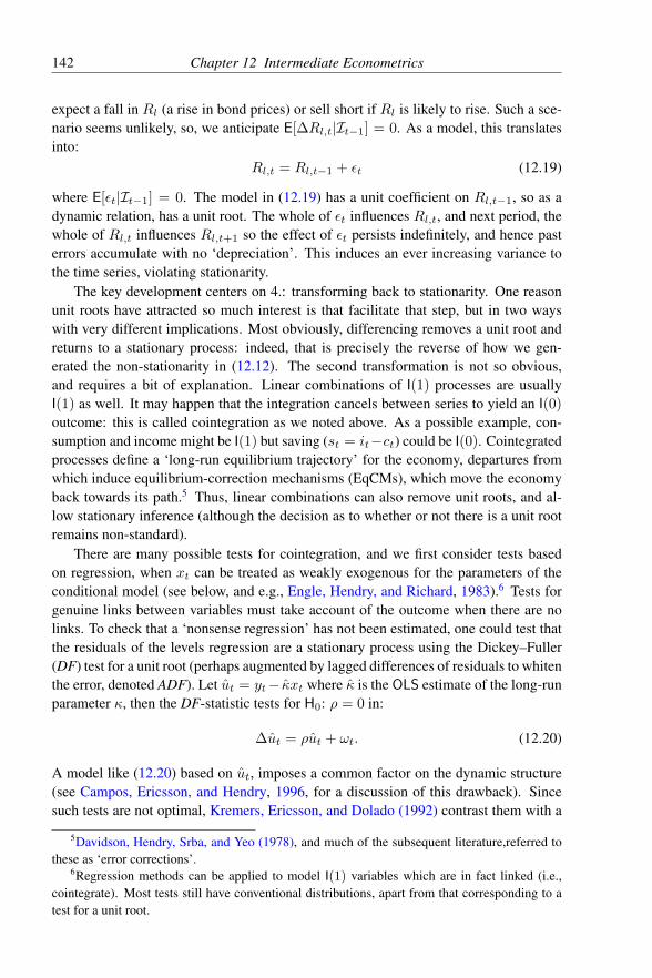
142 Chapter 12 Intermediate Econometrics
expect a fall in Rl (a rise in bond prices) or sell short if Rl is likely to rise. Such a sce-nario seems unlikely, so, we anticipate E[∆Rl,t|It−1] = 0. As a model, this translatesinto:
Rl,t = Rl,t−1 + εt (12.19)
where E[εt|It−1] = 0. The model in (12.19) has a unit coefficient on Rl,t−1, so as adynamic relation, has a unit root. The whole of εt influences Rl,t, and next period, thewhole of Rl,t influences Rl,t+1 so the effect of εt persists indefinitely, and hence pasterrors accumulate with no ‘depreciation’. This induces an ever increasing variance tothe time series, violating stationarity.
The key development centers on 4.: transforming back to stationarity. One reasonunit roots have attracted so much interest is that facilitate that step, but in two wayswith very different implications. Most obviously, differencing removes a unit root andreturns to a stationary process: indeed, that is precisely the reverse of how we gen-erated the non-stationarity in (12.12). The second transformation is not so obvious,and requires a bit of explanation. Linear combinations of I(1) processes are usuallyI(1) as well. It may happen that the integration cancels between series to yield an I(0)
outcome: this is called cointegration as we noted above. As a possible example, con-sumption and income might be I(1) but saving (st = it−ct) could be I(0). Cointegratedprocesses define a ‘long-run equilibrium trajectory’ for the economy, departures fromwhich induce equilibrium-correction mechanisms (EqCMs), which move the economyback towards its path.5 Thus, linear combinations can also remove unit roots, and al-low stationary inference (although the decision as to whether or not there is a unit rootremains non-standard).
There are many possible tests for cointegration, and we first consider tests basedon regression, when xt can be treated as weakly exogenous for the parameters of theconditional model (see below, and e.g., Engle, Hendry, and Richard, 1983).6 Tests forgenuine links between variables must take account of the outcome when there are nolinks. To check that a ‘nonsense regression’ has not been estimated, one could test thatthe residuals of the levels regression are a stationary process using the Dickey–Fuller(DF) test for a unit root (perhaps augmented by lagged differences of residuals to whitenthe error, denoted ADF). Let ut = yt− κxt where κ is the OLS estimate of the long-runparameter κ, then the DF-statistic tests for H0: ρ = 0 in:
∆ut = ρut + ωt. (12.20)
A model like (12.20) based on ut, imposes a common factor on the dynamic structure(see Campos, Ericsson, and Hendry, 1996, for a discussion of this drawback). Sincesuch tests are not optimal, Kremers, Ericsson, and Dolado (1992) contrast them with a
5Davidson, Hendry, Srba, and Yeo (1978), and much of the subsequent literature,referred tothese as ‘error corrections’.
6Regression methods can be applied to model I(1) variables which are in fact linked (i.e.,cointegrate). Most tests still have conventional distributions, apart from that corresponding to atest for a unit root.
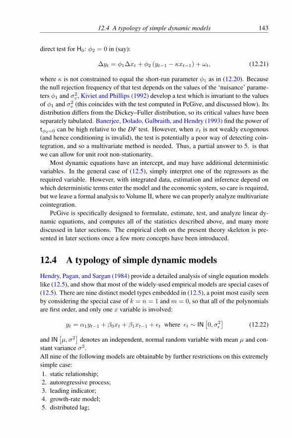
12.4 A typology of simple dynamic models 143
direct test for H0: φ2 = 0 in (say):
∆yt = φ1∆xt + φ2 (yt−1 − κxt−1) + ωt, (12.21)
where κ is not constrained to equal the short-run parameter φ1 as in (12.20). Becausethe null rejection frequency of that test depends on the values of the ‘nuisance’ parame-ters φ1 and σ2
v , Kiviet and Phillips (1992) develop a test which is invariant to the valuesof φ1 and σ2
v (this coincides with the test computed in PcGive, and discussed blow). Itsdistribution differs from the Dickey–Fuller distribution, so its critical values have beenseparately tabulated. Banerjee, Dolado, Galbraith, and Hendry (1993) find the power oftφ2=0 can be high relative to the DF test. However, when xt is not weakly exogenous(and hence conditioning is invalid), the test is potentially a poor way of detecting coin-tegration, and so a multivariate method is needed. Thus, a partial answer to 5. is thatwe can allow for unit root non-stationarity.
Most dynamic equations have an intercept, and may have additional deterministicvariables. In the general case of (12.5), simply interpret one of the regressors as therequired variable. However, with integrated data, estimation and inference depend onwhich deterministic terms enter the model and the economic system, so care is required,but we leave a formal analysis to Volume II, where we can properly analyze multivariatecointegration.
PcGive is specifically designed to formulate, estimate, test, and analyze linear dy-namic equations, and computes all of the statistics described above, and many morediscussed in later sections. The empirical cloth on the present theory skeleton is pre-sented in later sections once a few more concepts have been introduced.
12.4 A typology of simple dynamic modelsHendry, Pagan, and Sargan (1984) provide a detailed analysis of single equation modelslike (12.5), and show that most of the widely-used empirical models are special cases of(12.5). There are nine distinct model types embedded in (12.5), a point most easily seenby considering the special case of k = n = 1 and m = 0, so that all of the polynomialsare first order, and only one x variable is involved:
yt = α1yt−1 + β0xt + β1xt−1 + εt where εt ∼ IN[0, σ2
ε
](12.22)
and IN[µ, σ2
]denotes an independent, normal random variable with mean µ and con-
stant variance σ2.All nine of the following models are obtainable by further restrictions on this extremelysimple case:1. static relationship;2. autoregressive process;3. leading indicator;4. growth-rate model;5. distributed lag;

144 Chapter 12 Intermediate Econometrics
6. partial adjustment;7. autoregressive-error model (COMFAC);8. equilibrium-correction mechanism (EqCM);9. dead-start model.Equation (12.22) is a specialization of the special case of a linear, single-equation dy-namic model, with the apparently restrictive assumption that εt is a white-noise pro-cess. Yet most widely-used model types are schematically represented in (12.22), andthe typology highlights their distinct characteristics, strengths and weaknesses.
To clarify the approach, we consider the nine cases in turn, deriving each via re-strictions on the parameter vector:
θ′ = (α1, β0, β1)
of (12.22), noting that an intercept and an error variance can be included without alter-ing the implications in all models, and are omitted for simplicity of exposition. Four ofthe cases impose two restrictions on θ and five impose one, and these will be referredto respectively as one and two parameter models since σ2 is common to all stochasticmodels. Table 12.1 lists the outcomes.
Table 12.1 Model TypologyType of Model θ′ Entailed Restrictions on (12.22)static regression (0, β0, 0) α1 = β1 = 0 no dynamicsautoregressive process (α1, 0, 0) β0 = β1 = 0 no covariatesleading indicator (0, 0, β1) α1 = β0 = 0 no contemporaneitygrowth rate (1, β0,−β0) α1 = 1, no levels
β1 = −β0
distributed lag (0, β0, β1) α1 = 0 finite lagspartial adjustment (α1, β0, 0) β1 = 0 no lagged xautoregressive error (α1, β0,−α1β0) β1 = −α1β0 one common factor
error correction (α1, β0,K) K =β0 + β11− α1
long-run responsedead-start (α1, 0, β1) β0 = 0 lagged variables
Three important issues must be clarified before proceeding: the status of xt; thedependence of the model’s properties on the data properties; and whether each modeltype is being treated as correctly specified or as an approximation to a more generalDGP such as (12.5). These three problems arise in part because the analysis has notcommenced from the most general system needed to characterize the observed data ad-equately, and in part because the DGP is unknown in practice, so we do not know whichdata properties to take as salient features in an analytical treatment (not to mention inempirical studies). A system formulation is offered in Chapter 14.
For the present, we treat xt as if it were (weakly) exogenous for the parametersof interest in θ (see Engle, Hendry, and Richard, 1983, and §14.7.2). Heuristically,weak exogeneity ensures that we can take the conditioning variables as valid, and so

12.4 A typology of simple dynamic models 145
analyze the conditional equation (12.22) without loss of any relevant information aboutθ, despite not also modelling the process determining xt: this would be false if themodel of xt depended on θ. When xt in (12.22) is weakly exogenous for θ, then ifany member of the typology is valid, so must be every less restricted, but identifiable,member. That statement has profound implications not only for the general methodol-ogy of modelling, but also for such major issues of current contention as the practice of‘allowing for residual autocorrelation’, the validity of analyzing over-identified simul-taneous systems (the Sims critique: see Sims, 1980, and Hendry and Mizon, 1993), andthe imposition of restrictions based on prior theory, including the Lucas critique (seeLucas, 1976, Favero and Hendry, 1992, and Ericsson and Irons, 1995).
As noted earlier, xt is assumed to be I(1), and for convenience, we take ∆xt tobe a stationary process. This determines the answer to the second issue; but since someeconomic time series seem to be I(0) (e.g., unemployment), the case xt ∼ I (0) remainsrelevant. If xt and yt are cointegrated, then ut = (yt −Kxt) ∼ I (0), but such a beliefmay be false, and the case ut ∼ I (1) ∀K must be noted. The typology treats each casein turn, as if it were the correct specification, but notes both the historical success ofsuch an assumption, and the likely consequences when it is incorrect.
12.4.1 Static regression
Equations of the formyt = b0xt + ut
(with b0 and xt vectors in general) have played a large role in many macro-econometricsystems as erstwhile ‘structural’ equations (i.e., embodying the fundamental parame-ters of the behaviour of economic agents). In practice, ut has usually been highlyautocorrelated (reminiscent of nonsense correlations – see Yule, 1926), so that conven-tional inference about b0 is invalid (see, for example, Granger and Newbold, 1974, andPhillips, 1986). However, static equations reappeared as part of a two-stage strategyfor investigating cointegration, with the focus on testing whether or not ut was I(1)against the alternative that it was I(0) (see Engle and Granger, 1987). Then, b0 wouldbe a direct estimator of K in (12.9). Even so, the success of such an estimator in finitesamples has been questioned (see Banerjee, Dolado, Hendry, and Smith, 1986), and isdependent on the mean lag between y and x, noting that a static equation imposes thatmean lag at zero. Alternatively, the strategy of removing the autocorrelation in ut byfitting an autoregressive process is considered in §12.4.7. Finally, viewed as a structuralequation, all of the restrictions on dynamics and covariates are testable against (12.5),as are the implicit restrictions highlighted in §14.7.
12.4.2 Univariate autoregressive processes
The equationyt = a1yt−1 + et
serves as our representative of univariate time-series models (see Box and Jenkins,1976). If yt is I(1), a1 = 1, inducing a random walk when et is white noise. Autore-
146 Chapter 12 Intermediate Econometrics
gressive equations are widely used for ex ante forecasting, and have proved a powerfulchallenger to econometrics systems in that domain (see, for example, Nelson, 1972, andthe vector analogues in Doan, Litterman, and Sims, 1984; see Clements and Hendry;Clements and Hendry, 1998, 1999, for an explanation based on other sources of non-stationarity than unit roots). In economics, the interdependence of economic decisions(for example, one person’s income is another’s expenditure) entails that univariate au-toregressions must be derived, and hence are not autonomous processes – where anequation for yt is autonomous if changes in the process generating xt do not alter it.Here, the autoregression is obtained by eliminating, or marginalizing with respect to,xt. For example, let xt = xt−1 + νt where νt ∼ IN
[0, σ2
t
]when in fact α1 = 1
and β1 = −β0 in (12.22), then yt = yt−1 + εt + β0νt has a non-constant varianceσ2ε + β2
0σ2t . Consequently, econometric models should both fit better than autoregres-
sions (or else they are at least dynamically mis-specified), and should forecast better (orelse the constancy of the econometric model must be suspect).
That both these requirements are sometimes not satisfied is owing in part to theinappropriateness of some current empirical methodological practices. A major objec-tive of PcGive is to offer an alternative approach which circumvents such difficultiesby commencing from a general dynamic specification that automatically embeds therelevant special cases.
12.4.3 Leading indicators
Models of the formyt = c1xt−1 + vt
can be used in forecasting if x leads y with sufficient reliability (for example, ordersarrive ahead of output). In the absence of a sound behavioural theory, however, c1 neednot be constant. If it is not, that will lead to poor forecasting, especially in periodsof change when good forecasts are most needed. Moreover, there seems no good rea-son for excluding lagged ys, and if a general dynamic model is postulated, then theeconometric considerations in §14.5, §14.7, §14.6 and §14.8.2 apply: see Emerson andHendry (1996) and Clements and Hendry (1998).
12.4.4 Growth-rate models
The evolutionary and trend-like behaviour of many economic time series led earlierinvestigators to recommend differencing data prior to statistical analysis. One exampleis Granger and Newbold (1977) although, as argued in Hendry and Anderson (1977),there are other transformations (such as ratios) which potentially could also removetrends. That leads on to the concept of cointegration discussed in §12.4.8.
Growth-rate models have the form
∆yt = d0∆xt + ηt.
Such models successfully avoid nonsense regressions problems in I(1) data, and fromthe transformed dependent variable, a useful measure of goodness of fit can be calcu-lated. Nevertheless, if the variance of ∆xt is large relative to that of ∆yt, d0 must be
12.4 A typology of simple dynamic models 147
small even if yt and xt are cointegrated withK = 1 (this is the permanent income issuein one guise: see Davidson, Hendry, Srba, and Yeo, 1978). Further, although yt = Kxtimplies ∆yt = K∆xt, the converse is false in a stochastic world owing to integratingthe error.
Alternatively, there are no a priori grounds for excluding levels from economicrelationships since initial disequilibria cannot be assumed to be irrelevant: that is, thetime path of ∆yt for a given sequence ∆xt may depend on the relationship between y0
and x0. Two further insights into the drawbacks of growth-rate models are discussedbelow in §12.4.7 and §12.4.8.
On the methodological level, a mistake sometimes committed in applied economicsis to begin with a linear approximation to a steady-state theory of the form: yt =
f (xt), fit a static model thereto, discover severe residual autocorrelation and ‘correct’that, either by differencing, or by using ‘Cochrane–Orcutt’ (but see their 1949 article,Cochrane and Orcutt, 1949, which does not recommend that procedure, as noted byGilbert, 1989) but finding an autoregressive parameter near unity. While the goodnessof fit may not be greatly worsened by imposing differencing, dynamic responses can besubstantially distorted, and ignoring long-run feedbacks may distort policy strategies.
12.4.5 Distributed lags
Although using only one lag makes the resulting model highly schematic, but neverthe-less the equation
yt = f0xt + f1xt−1 + ξt,
is representative of the class of finite distributed lags. Such models remain open tothe objections noted in §12.4.1 above, are highly dependent on whether xt is weakly,or strongly, exogenous unless ξt is white noise (which in practice it rarely is in thisclass), and tend to suffer from collinearity owing to the inappropriate parametrizationof including many levels of the regressor (see Chapter 15). Imposing so-called a priorirestrictions on the lag coefficients to reduce the profligate parametrization has little torecommend it, although such restrictions are at least potentially testable. It is hard tosee any theoretical grounds for excluding lagged ys, given that they are another wayof representing a distributed lag relationship; and as shown in §12.4.7, considerabledangers exist in arbitrarily removing any residual autocorrelation from ξt.
12.4.6 Partial adjustment
The equationyt = g0xt + g1yt−1 + ζt
occurs regularly in empirical macro-economics, and can be derived from assuming along-run desired target of the form yt = Kxt subject to quadratic adjustment costs(see, for example, Eisner and Strotz, 1963, and Nickell, 1985). While such a modeltype seems reasonable in principle, it does not entail that the y and x variables whichagents use in their decision rules are precisely the levels analyzed by the economist.

148 Chapter 12 Intermediate Econometrics
For example, agents may use the (log of the) consumption-income ratio as their yt, andthe growth rate of income as their xt, rather than the levels of both.7 The resultingeconometric specification, however, is wholly different despite the common element ofpartial adjustment.
Even when yt and xt are cointegrated in levels, the partial adjustment model haslittle to recommend it unless it happens to coincide with the DGP. The mean lag isg1/ (1− g1) whereas the median lag (the number of periods to reach the half-way stagetowards equilibrium) is zero for g0 ≤ 1
2 and is − log (2g1) / log (g1) for g0 > 12 , so
that a skewed distribution is imposed irrespective of the data (see, for example, Hendry,1995a, for the derivation of these formulae). When g1 is near unity, both measuresentail extremely slow adjustment, exacerbated by any untreated positive residual auto-correlation. Further, xt and yt−1 are usually highly correlated, so again an unfortunateparametrization is being selected. Since there are no good arguments for a priori ex-cluding all the lagged xs, and plenty of empirical evidence to show that they do matterin many cases, this model type again seems suspect.8
12.4.7 Autoregressive errors or COMFAC models
As noted in §12.2, some of the roots of a (L) and b (L) in (12.4) may be equal, allowingcancellation. In the case of (12.22) with β0 6= 0, we can write the equation as:
(1− α1L) yt = β0
(1 +
β1
β0L
)xt + εt.
Thus, if and only if α1 = −β1/β0 or β1 + α1β0 = 0, then on dividing both sides by(1− α1L), the equation can be rewritten as:
yt = β0xt +εt
(1− α1L),
or letting ρ = α1:
yt = β0xt + ut where ut = ρut−1 + εt, (12.23)
yielding a static model with an autoregressive error. The term (1− α1L) is a factor(in this simple case, the only factor) of a (L) and similarly (1 + (β1/β0)L) is a factorof b (L), so that when these are equal there is a factor in common in a (L) and b (L)
(leading to the name COMFAC). The converse that (12.23) induces a common factor isobvious, so there is an isomorphism between autoregressive errors and common factorsin the lag polynomials: if you believe one, you must believe the other. Since (12.23)imposes restrictions on (12.22), these are testable, and rejection entails discarding thesupposed reduction to (12.23) (see Hendry and Mizon, 1978). Thus, the ADL classincludes all models with autoregressive errors.
7The latter anyway seems suspect since few consumers appear to suffer great adjustment costsin response to increases in their expenditure when income has risen.
8Lags would arise naturally in the postulated model if the agents’ y and x were not the levelsthe economist selects.
12.4 A typology of simple dynamic models 149
Perhaps the greatest non sequitur in the history of econometrics is the assumptionthat autocorrelated residuals entail autoregressive errors, as is entailed in ‘correctingserial correlation using Cochrane–Orcutt’. Dozens of mis-specifications in time-seriesdata will induce residual autocorrelation without corresponding to common factors inthe lag polynomials of the underlying general model (12.4). Indeed, the order of testingis incorrect: to estimate any models like (12.23) first necessitates establishing the valid-ity of (12.4), then showing that a (L) and b (L) have common factors, and finally testingH0: ρ = 0. Showing that ρ 6= 0 in equations like (12.23) does not prove that there arevalid common-factor restrictions. PcGive offers algorithms for testing common-factorrestrictions in equations like (12.5) using the Wald-test approach in Sargan (1980b). Ifsuch restrictions are accepted, generalizations of (12.23) are estimable using the RALSestimator described in Chapter 17.
Two points of importance from (12.23) are that: (a) it imposes a zero mean lagirrespective of the actual lag responses, since the short-run and long-run responses areforced to be equal by the choice of model type; and (b) the growth-rate model of §12.4.4can be reinterpreted as imposing a common factor then setting ρ to unity. We concurwith the advice in the title of the paper by Mizon (1995).
12.4.8 Equilibrium-correction mechanisms
The issue of appropriate reparametrizations of θ has arisen on several occasions above,and many alternatives are conceivable. One natural choice follows from rearranging(12.22) as:
∆yt = (α1 − 1) yt−1 + β0∆xt + (β1 + β0)xt−1 + εt= β0∆xt + (α1 − 1) (yt−1 −Kxt−1) + εt,
(12.24)
where K = (β0 + β1) / (1− α1) is the long-run response in (12.9) above whenα1 6= 1. The new parameters in f (θ) = ψ = (β0, (1− α1) ,K)
′ correspond to the im-pact effect, the feedback effect and the long-run response: no restrictions are imposed inthis transformation. The term (y −Kx)t−1 was called an error-correction mechanism(EqCM) in Davidson, Hendry, Srba, and Yeo (1978) since it reflected the deviation fromthe long-run equilibrium outcome, with agents correcting (1− α1) of the resulting dis-equilibrium each period. However, such a mechanism does not error correct betweenequilibria, so equilibrium-correction mechanism is more apposite – and has the sameacronym (but is more often written EqCM). Sargan (1964) provides a real-wage exam-ple, and Hendry and Anderson (1977) considered some non-unit EqCMs. The specialcase K = 1 is of interest in econometrics as it corresponds to long-run proportionality(or homogeneity in log-linear models), but EqCMs are well defined for K 6= 1, al-though usually K will then need to be estimated. As Hendry, Pagan, and Sargan (1984)note, logistic formulations or more general functions may be necessary to model agents’behaviour if they adjust more or less rapidly depending on the extent of disequilibrium(see Escribano, 1985).
Engle and Granger (1987) establish an isomorphism between EqCMs and coin-tegrated processes: if yt and xt are each I(1) and are cointegrated, then there exists

150 Chapter 12 Intermediate Econometrics
an EqCM of the form (y −Kx) and conversely. The former does not entail that theEqCM necessarily enters the yt equation, rather than the xt equation, and may enterboth (which would violate weak exogeneity: see Hendry and Mizon (1993) for an ex-ample).
In our simple typology, the only EqCM case to impose any restrictions on (12.24) isK = 1 or α1 + β0 + β1 = 1, revealing that all long-run proportionality theories can bereproduced in static equilibrium by an appropriate EqCM. Here, this restriction yields:
∆yt = γ0∆xt − γ1 (y − x)t−1 + ωt. (12.25)
Thus, another interpretation of the growth-rate model §12.4.4 is revealed, namely, itcorresponds to imposing long-run homogeneity (α1 + β0 + β1 = 1) and the absenceof feedback from the level (1− α1 = 0), which together entail a unit root. Conse-quently, small values of γ0 are compatible with long-run proportionality. Since partialadjustment corresponds to the special case where x = y∗ (the desired target), it imposesγ0 = −γ1 to exclude the lagged x.
The parametrization in (12.25) has several advantages beyond being more inter-pretable: the regressors ∆xt and (y − x)t−1 will not usually be highly correlated, be-ing a current change and a lagged disequilibrium; and proportionality is easily tested byadding xt−1 as a (relatively non-collinear) regressor (however, such a test must allowfor the possibility that xt may be I (1)). Further, a less strong lag shape is being im-posed, since the mean lag is (1− γ0) /γ1, which depends on both parameters, and canbe small even if (1− γ1) is around 0.9, whereas the median lag is zero for γ0 ≥ 1
2 andis − log 2 (1− γ0) / log (1− γ1) for γ0 <
12 .
When the EqCM is the correct specification, the partial adjustment model may suf-fer from severe biases, and possibly residual autocorrelation, since it omits xt−1 whichis highly correlated with xt: because the coefficients of xt and xt−1 are of similarmagnitudes but opposite signs, this will drive the coefficient of xt in the partial adjust-ment model close to zero (a common empirical problem), so that g0 ' 1 − g1 results.Note that β1 < 0 in (12.22) need not entail any negative weights wi in the solvedrepresentation:
yt =
∞∑i=0
wixt−i + ut.
Thus, do not delete lagged xs because their coefficients appear to have ‘wrong signs’,since on a reparametrization they may have the correct sign.
Finally, EqCMs can be confused with COMFAC models despite their very differentimplications for lag responses. This arises because COMFAC is an EqCM with therestriction that long-run and short-run responses are equal, as can be seen by rewriting(12.23) in the form:
yt = β0xt + ρ (yt−1 − β0xt−1) + εt,
or:∆yt = β0∆xt + (ρ− 1) (y − β0x)t−1 + εt. (12.26)

12.5 Interpreting linear models 151
Thus, the degree of mis-specification of (12.26) for (12.24) depends on the extent towhich (α1 − 1) (K − β0) 6= 0, which could be small even if K = 1 and, for example,β0 = 0.4. Nevertheless, despite (12.24) and (12.26) having similar goodness of fit, themean lag in (12.24) when K = 1 could be large at the same time as (12.26) imposes itat zero.
12.4.9 Dead-start models
The main consideration arising for this type of model is its exclusion of contemporane-ous information. This could be because:
yt = α1yt−1 + β1xt−1 + εt (12.27)
is structural, and hence is a partial adjustment type. Alternatively, (12.27) could be aderived form, from which xt has been eliminated, in which case (12.27) is unlikely tobe autonomous, and its parameters would be susceptible to alter with changes in thebehaviour of the xt process. In this second case, the coefficients are not interpretablesince they are (unknown) functions of the correlations between xt and (yt−1, xt−1).
Care is obviously required in selecting an appropriate type of model to characterizeboth a given theory and the associated data; some of the methodological considerationsdiscussed below help clarify that choice.
12.5 Interpreting linear modelsThe notation for the linear model is the same as that in Chapter 13:
yt =
k∑i=1
βixi,t + εt = β′xt + εt with εt ∼ IN[0, σ2
ε
], (12.28)
where β is k × 1 and E [xtεt] = 0. Grouping all the T observations:
y = Xβ + ε with ε ∼ N[0, σ2
ε IT]
(12.29)
where y,X, ε are respectively T × 1, T × k and T × 1.First, we discuss the four distinct interpretations of (12.28), see Richard (1980) or
Hendry, Pagan, and Sargan (1984):
12.5.1 Interpretation 1: a regression equation
A regression is the conditional expectation of yt given xt (denoted by E [yt|xt]). Takingthe conditional expectation in (12.28):
E [yt | xt] = β′xt (12.30)
where β is a parameter of interest. Sufficient conditions to sustain that interpretationof (12.28) are a jointly stationary, multivariate-normal distribution for (yt,xt) with xt

152 Chapter 12 Intermediate Econometrics
weakly exogenous for β. (A formal derivation of a conditional equation in a bivariatenormal distribution is provided in Chapter 13. The properties of regression estimatorsare also discussed in that chapter: for example, that V [yt − β′xt] is minimized by thechoice of β). Notice that the minimal conditions which needed to justify (12.30) arenot sufficient to sustain E [y|X] = Xβ, which is used in Chapter 13, as that involvesconditioning past ys on future xs.
12.5.2 Interpretation 2: a (linear) least-squares approximation
Here, the approximation is to a postulated general function:
yt = f (xt) + et,
chosen on the criteria that: (a) (12.28) is linear in xt; and (b)∑Tt=1 ε
2t is to be min-
imized. Graphically, β in (12.28) is not ∂f/∂x′ (the tangent), owing to the secondcriterion, but must be a chord. If εt is non-normal, the regression would not be lin-ear, whereas a linear approximation must be, so §12.5.1 and §12.5.2 are distinct. If,in practice, f is non-linear then (12.28) may be a poor approximation, εt could beautocorrelated, and forecasts could be poor (since ∂f/∂x′t need not be constant). Ofcourse, a quadratic or even a higher-order approximation to f (x) could be used. White(1980) provides a formal analysis of this case.
12.5.3 Interpretation 3: an autonomous contingent plan
In this interpretation:ypt = x′tβ,
is the planned value and:yt = ypt + ut,
is the outcome, which deviates randomly from the plan (see Marschak, 1953, Bentzeland Hansen, 1955, and Hendry and Richard, 1983). Thus, (12.28) characterizes howagents form plans, and β is an invariant parameter (see Frisch, 1938). Since ut neednot have a joint normal distribution, §12.5.3 and §12.5.1 are different; and f (x) mightbe approximated by a non-linear function of xt, so §12.5.2 and §12.5.3 also differ. Forexample, autoregressive-conditional heteroscedastic (ARCH) errors (so the variance attime t depends on the variance at time t − 1) would be one instance where ut is notjointly normal, in which case, E [y|X] 6= Xβ need not hold although (12.28) could stillbe correct.
12.5.4 Interpretation 4: derived from a behavioural relationship
The final interpretation is:
E [yt | It−1] = β′E [xt | It−1] ,
or:ypt = β′xet ,

12.6 Multiple regression 153
where It−1 denotes the universe of information available to agents at the time theirplans are formulated. Here, the distinction is drawn between a plan (which is madeabout a variable that the relevant agent controls), and an expectation (which is formedabout an uncontrolled variable). Let νt = xt − xet and ηt = yt − ypt be the vector ofexpectational errors and the departure of the outcome from the plan respectively, withE [νt|It−1] = 0 and E [ηt|It−1] = 0, then:
yt = β′xt + εt with εt = ηt − β′νt,
so that E [εt|It−1] = 0 but E [εt|xt] 6= 0 owing to their sharing the common componentνt. In this setting, regression is inconsistent (and biased) for the parameter of interestβ, and may deliver non-constant estimates even when β is invariant when the processdetermining xt alters. Clearly, §12.5.4 is distinct from §12.5.1–§12.5.3.
Merely asserting yt = β′xt + εt is not an adequate basis for econometric analysis,given the four distinct interpretations of equation (12.28) just described. Although thefour interpretations happen to coincide in stationary, linear models with normal errors,the distinctions in §12.5.1–§12.5.4 are not formal: in practice, which one is valid entailsquite different prognoses for the success (or failure) of any empirical study. When the xtprocess varies enough, some discrimination is possible owing to the non-constancy ofβ, and this is both the usual situation and that in which discrimination actually matters.
12.6 Multiple regressionThe algebra of least-squares estimation is established in matrix notation in Chap-ter 13, and we merely record some of the most relevant formulae here. First, theOLS coefficient estimates and their estimated variances are:
β = (X′X)−1
X′y withV[β]
= σ2ε (X′X)
−1.
Also the error variance estimate and the residual sum of squares are:
σ2ε =
RSS
(T − k)when RSS =
(y −Xβ
)′ (y −Xβ
).
Further, M = IT−X (X′X)−1
X′ is a symmetric, idempotent matrix which annihilatesX, so MX = 0 implying My = Mε = u (the vector of residuals y −Xβ). Tests ofH0: β = 0, or components thereof, are developed in Chapter 13. A simple empiricalexample with a constant and two other regressors is presented in §11.10.
It is a brave (foolhardy?) investigator who deems their model to coincide with theDGP, and most econometricians consider the possibility of various mis-specificationswhen appraising empirical research. A number of possibilities can be shown alge-braically, such as omitting a relevant regressor. Denoting the OLS estimator of the mis-specified model by , partition X = (Xa : Xb), and conformably let β = (β′a : β′b)
′
which are ka × 1 and kb × 1 so that ka + kb = k. Then:
β = (X′aXa)−1
X′ay and˜
V[βa
]= σ2
ε (X′aXa)−1 when σ2
ε =y′May
(T − ka),

154 Chapter 12 Intermediate Econometrics
and Ma has the same form as M but using only Xa. Partitioned inversion of (X′X)
leads to the important numerical identity that:
βa ≡ βa + Bβb where B = (X′aXa)−1
X′aXb.
If xt is a stationary stochastic process, then:
E[σ2ε
]≥ E
[σ2ε
],
since there is a component of xb,t in the residual. Both the bias in βa and in the errorvariance were illustrated by the comparative regression results in §11.10. Tests for thesignificance of omitted variables can be undertaken from the Test menu; what wouldyou conclude after getting significant test results for two different choices?
Despite a high correlation between xa,t and x, it is possible that:
V[β]<
˜V[βa
],
owing to the reduction in σ2ε from σ2
ε when xb,t is added to the regression of yt on xa,t.A more extensive treatment of collinearity is provided in Chapter 15.
12.6.1 Estimating partial adjustment
All these issues can be illustrated empirically, and we do so using the artificial dataset called data.in7 and data.bn7, with the four variables CONS, INC, INFLAT andOUTPUT. The first regression is of CONS on INC and CONS lagged (that is, a partialadjustment form) which yields:9
EQ(1) Modelling CONS by OLS (using data.in7)The estimation sample is: 1953 (2) to 1992 (3)
Coefficient Std.Error t-value t-prob Part.R^2CONS_1 0.823870 0.03300 25.0 0.000 0.8008Constant -45.6043 14.65 -3.11 0.002 0.0589INC 0.223975 0.04158 5.39 0.000 0.1577
sigma 2.03715 RSS 643.24383R^2 0.977627 F(2,155) = 3387 [0.000]**Adj.R^2 0.977339 log-likelihood -335.103no. of observations 158 no. of parameters 3mean(CONS) 875.848 se(CONS) 13.5326
AR 1-5 test: F(5,150) = 14.442 [0.0000]**ARCH 1-4 test: F(4,150) = 20.581 [0.0000]**Normality test: Chi^2(2) = 4.2396 [0.1201]Hetero test: F(4,153) = 2.7848 [0.0286]*Hetero-X test: F(5,152) = 2.2154 [0.0556]RESET23 test: F(2,153) = 4.0817 [0.0188]*
At first sight, the coefficients seem well determined, and the long-run effect of INC onCONS is close to unity. However, the test summary indicates problems. We will returnto testing the specification in the next section.
9The exact form of the output depends on the options settings.

12.6 Multiple regression 155
12.6.2 Heteroscedastic-consistent standard errors
Since residual autocorrelation and residual heteroscedasticity both bias estimated co-efficient standard errors, corrections have been developed. These can be computed inPcGive by selecting Test, Further output, which yields:
Heteroscedasticity consistent standard errorsCoefficients SE HACSE HCSE JHCSE
CONS_1 0.82387 0.033004 0.048736 0.032659 0.033110Constant -45.604 14.647 19.361 13.642 13.778INC 0.22398 0.041582 0.062002 0.040992 0.041563
Coefficients t-SE t-HACSE t-HCSE t-JHCSECONS_1 0.82387 24.962 16.905 25.226 24.883Constant -45.604 -3.1135 -2.3554 -3.3428 -3.3100INC 0.22398 5.3864 3.6124 5.4638 5.3889
The column above labelled HCSE denotes heteroscedastic-consistent standard er-rors (see Eicker, 1967, and White, 1980). Relative to the usual standard errors reportedfor regression estimation, HCSEs reflect any heteroscedasticity in the residuals whichis related to the regressors. Consider OLS estimation in (12.28) when εt ∼ IN
[0, σ2
t
]with E [xtεs] = 0 ∀t, s,but we mistakenly believe that:
εt hIN[0, σ2
ε
],
whereh
denotes ‘is hypothesized to be distributed as’. To estimate β, we set to zero:
T∑t=1
xtεt = 0. (12.31)
Then, to derive the variance, we would analytically calculate:
E
T∑t=1
xtεt
(T∑t=1
xtεt
)′ = E
[T∑t=1
T∑s=1
xtεtεsx′s
]=
T∑t=1
σ2t xtx
′t,
from which the variance of β is given by:
V = V[β]
= (X′X)−1
(T∑t=1
σ2t xtx
′t
)(X′X)
−1. (12.32)
This involves a weighted average of the xs with weights σ2t proportional to the het-
eroscedastic error variances. The conventional variance estimator is:
V[β]
= σε
(T∑t=1
xtx′t
)−1
.
When the weights σ2t in (12.32) are not constant, the conventional variance estimator
does not correctly reflect the estimation uncertainty.

156 Chapter 12 Intermediate Econometrics
Surprisingly, the correct variance formula in (12.32) can be estimated from the sam-ple by replacing the unknown σ2
t by ε2t (see White, 1980):
V = (X′X)−1
(T∑t=1
ε2txtx′t
)(X′X)
−1. (12.33)
V is consistent for V (see White, 1980) and the conventional estimator of V ariseswhen all
σ2t
are constant. The square roots of the diagonal of V are the HCSEs
above. When these are close to the OLS SEs, there is little evidence of distortion ofinference from untreated heteroscedasticity. The JHCSEs denote Jackknife corrections(see MacKinnon and White, 1985).
Similarly, generalizations to allow for error autocorrelation have been obtained, andare reported above as HACSEs (see Newey and West, 1987 and Andrews, 1991). How-ever, in both cases in must be remembered that residual autocorrelation and residualheteroscedasticity may derive from dozens of causes, unrelated to the errors. In thesecommon cases, the various forms of HCSE, HACSE etc. will not be useful – theymerely serve to camouflage model mis-specification, not improve inference.
All reported statistics depend on assumptions about how well the model describesthe data, and until these assumptions are established as valid, the interpretation ofany empirical output is unclear. In the previous chapter, we considered the many as-sumptions made to derive the distribution of ‘t’-tests : the assumptions for HCSEs areweaker, but nonetheless strong – as just seen. As a first pass, we use Test, Graphical
analysis to visually investigate the fit, the residuals, the residual correlogram, and thedensity of the residuals. The outcome is shown in Figure 12.1 and reveals a fair fit, butdistinct residual autocorrelation, as well as a major group of ‘outliers’ in the residualsaround 1973–4 (does this historical period ring any warning bells?).
More formal mis-specification tests will be considered shortly, but the graph showssubstantial residual autocorrelation. How to proceed now?
12.6.3 Specific-to-general
To test a specification, investigators often add extra variables, so we first include laggedINC to obtain:
EQ(2) Modelling CONS by OLS (using data.in7)The estimation sample is: 1953 (2) to 1992 (3)
Coefficient Std.Error t-value t-prob Part.R^2CONS_1 0.985875 0.02762 35.7 0.000 0.8922Constant 2.51140 11.39 0.220 0.826 0.0003INC 0.495844 0.03797 13.1 0.000 0.5255INC_1 -0.484913 0.04103 -11.8 0.000 0.4756
sigma 1.47998 RSS 337.313361R^2 0.988268 F(3,154) = 4324 [0.000]**Adj.R^2 0.988039 log-likelihood -284.107no. of observations 158 no. of parameters 4mean(CONS) 875.848 se(CONS) 13.5326

12.6 Multiple regression 157
CONS Fitted
1960 1970 1980 1990
860
880
900CONS Fitted CONS × Fitted
860 870 880 890
860
880
900CONS × Fitted
r:CONS (scaled)
1960 1970 1980 1990
-2.5
0.0
2.5 r:CONS (scaled) r:CONS N(0,1)
-4 -2 0 2 4
0.2
0.4
Densityr:CONS N(0,1)
ACF-r:CONS
0 5 10
0
1ACF-r:CONS r:CONS
-4 -2 0 2 4
-2.5
0.0
2.5
5.0 Distributionr:CONS
Figure 12.1 Goodness-of-fit measures for partial adjustment model
The added variable is highly significant, and so invalidates the first partial-adjustmentmodel. The standard errors of both CONS and INC have fallen, despite adding thecollinear variable INC 1, mainly because s has fallen markedly. Consistent with thatfeature, the partial r2 values have increased.
Unfortunately, the model appears to have a common factor of unity suggesting thatCONS and INC are not cointegrated (the lagged dependent variable coefficient is nearunity, and the coefficients on INC and INC lagged are equal magnitude opposite sign).Three formal tests are possible, assuming the model is a good data description. First,we test for a common factor (Dynamic analysis, Test for common factors) to obtain:
COMFAC Wald test statistic table, COMFAC F(1,154) = 0.0306861 [0.8612]Order Cumulative tests Incremental tests1 Chi^2(1) = 0.030686 [0.8609] Chi^2(1) = 0.030686 [0.8609]
The test easily accepts, so the model is now COMFAC rather than partial adjustment.The calculated values of the roots are also shown, and these are close to unity. Thus,we next test for a unit root by seeing if all the coefficients (other than the constant) addto unity: the linear restrictions test yields:
Test for linear restrictions (Rb=r):R matrix
CONS_1 Constant INC INC_11.0000 0.00000 1.0000 1.0000
r vector1.0000
LinRes F(1,154) = 0.0648135 [0.7994]

158 Chapter 12 Intermediate Econometrics
This too accepts with ease. This suggests it is worth conducting the PcGive unit-roottest (see Banerjee and Hendry, 1992) (from the Test menu, Dynamic analysis, reportedonly in part here):
Tests on the significance of each variableVariable F-test Value [ Prob] Unit-root t-testCONS F(1,154) = 1274.1 [0.0000]** -0.51143Constant F(1,154) = 0.048588 [0.8258]INC F(2,154) = 97.321 [0.0000]** 0.31073
Finally, the solved long run is badly determined and the unit-root test does not reject.All the evidence meshes: CONS and INC do not cointegrate.
Solved static long run equation for CONSCoefficient Std.Error t-value t-prob
Constant 177.794 1022. 0.174 0.862INC 0.773850 1.159 0.667 0.505Long-run sigma = 104.775
ECM = CONS - 177.794 - 0.77385*INC;WALD test: Chi^2(1) = 0.445497 [0.5045]
Again one must ask: how valid are these tests? A glance at the graphical diagnostics(corresponding to Figure 12.1) shows that the residual autocorrelation has not improved,so none of the SEs is reliable. More formal mis-specification tests are provided in theTest summary, and yield:
AR 1-5 test: F(5,149) = 7.8187 [0.0000]**ARCH 1-4 test: F(4,150) = 6.2829 [0.0001]**Normality test: Chi^2(2) = 7.6549 [0.0218]*Hetero test: F(6,151) = 1.0948 [0.3681]Hetero-X test: F(9,148) = 1.0733 [0.3859]RESET23 test: F(2,152) = 2.9783 [0.0539]
There is indeed significant residual autocorrelation, and apparently autoregressive con-ditional heteroscedasticity (ARCH) as well (see Engle, 1982). However, the latter couldbe caused by the former (see Engle, Hendry, and Trumbull, 1985), and merely shows thedifficulty of interpreting outcomes when several tests reject. If we test for the omissionfrom the equation of the remaining two variables in the database, we obtain:
Omitted variables test: F(2,152) = 67.5992 [0.0000] **Added variables:[0] = INFLAT[1] = OUTPUT
Both seem to matter! All previous results are invalidated: how to proceed now? Doesthis explain the earlier problems? – or do they explain the latest results? or do further‘untreated problems’ lurk unseen?
12.6 Multiple regression 159
12.6.4 General-to-specific (Gets)
It is precisely conundrums of the form just encountered that have led us to suggestan alternative approach to modelling. If at some stage you intend to investigate therelevance of a given phenomenon (for example, lagged INC, or INFLAT), include itin the model from the outset if sample size allows: this leads to general-to-specificmodelling (or Gets), discussed in greater detail in Chapter 15.
The initial general model should contain all the effects likely to be relevant, in-cluding sufficient lags to ensure no residual autocorrelation, then be tested for its va-lidity. Once that has been established, further testing can proceed in confidence thatconflicts will not arise. To illustrate, consider as an initial starting point a model involv-ing CONS, INC, and INFLAT, adding their one-period lags:
EQ( 3) Modelling CONS by OLS (using data.in7)The estimation sample is: 1953 (2) to 1992 (3)
Coefficient Std.Error t-value t-prob Part.R^2CONS_1 0.798310 0.02716 29.4 0.000 0.8504Constant -20.2695 8.526 -2.38 0.019 0.0358INC 0.498937 0.02833 17.6 0.000 0.6711INC_1 -0.276105 0.03788 -7.29 0.000 0.2590INFLAT -0.793095 0.1840 -4.31 0.000 0.1090INFLAT_1 -0.250612 0.2031 -1.23 0.219 0.0099
sigma 1.07836 RSS 176.753411R^2 0.993852 F(5,152) = 4915 [0.000]**Adj.R^2 0.99365 log-likelihood -233.053no. of observations 158 no. of parameters 6mean(CONS) 875.848 se(CONS) 13.5326
The standard errors are much smaller than any previous results, and partial R2 arehigher, although the correlations between the regressors are quite large:
Correlation matrixCONS CONS_1 INC INC_1 INFLAT
CONS 1.000CONS_1 0.9866 1.000INC 0.9422 0.9310 1.000INC_1 0.9144 0.9414 0.9510 1.000INFLAT -0.3511 -0.2756 -0.1271 -0.07332 1.000INFLAT_1 -0.4174 -0.3405 -0.1953 -0.1124 0.9266
Seven correlations exceed 0.9, yet every coefficient in the regression is well determined,although some are small. For example, the longest lag on INFLAT is irrelevant andcould be eliminated. The goodness of fit as measured by s is 50% less than for the firstequation, so the general model provides a usable baseline.
Next we test for a common factor:
COMFAC Wald test statistic table, COMFAC F(2,152) = 53.1042 [0.0000] **Order Cumulative tests Incremental tests1 Chi^2(2) = 106.21 [0.0000]** Chi^2(2) = 106.21 [0.0000]**
Roots of lag polynomials:

160 Chapter 12 Intermediate Econometrics
real imag modulusCONS 0.79831 0.00000 0.79831INC 0.55339 0.00000 0.55339INFLAT -0.31599 0.00000 0.31599
The COMFAC test strongly rejects, and the roots are now well below unity in absolutevalue.10 Correspondingly, the long run is well determined, and the unit-root test rejectsthe null, so cointegration is obtained between CONS, INC and INFLAT:
Solved static long run equation for CONSCoefficient Std.Error t-value t-prob
Constant -100.498 37.53 -2.68 0.008INC 1.10482 0.04185 26.4 0.000INFLAT -5.17480 0.5224 -9.91 0.000Long-run sigma = 5.3466
ECM = CONS + 100.498 - 1.10482*INC + 5.1748*INFLAT;WALD test: Chi^2(2) = 962.504 [0.0000] **
Tests on the significance of each variableVariable F-test Value [ Prob] Unit-root t-testCONS F(1,152) = 863.96 [0.0000]** -7.4261**Constant F(1,152) = 5.6515 [0.0187]*INC F(2,152) = 159.04 [0.0000]** 6.8393INFLAT F(2,152) = 69.037 [0.0000]** -11.1
The model satisfies all the statistics in the diagnostic test summary, and Figure 12.2shows the improved graphical performance: with a little experience, a glance at Figure12.1 shows a failed model, whereas Figure 12.2 is fine. Hopefully, your experience isgrowing rapidly.
12.6.5 Automatic model selection using Autometrics
Automatic model selection is a recent addition to the toolkit of the applied econometri-cian. When the initial model is large, general-to-specific modelling (Gets), as describedin the previous section, can be very time consuming. There may be many paths thatprovide a valid reduction. At the same time it is necessary to keep checking the validityof each reduction (i.e. to maintain congruency, see §12.10.2). The computer implemen-tation of Gets provides a convenient solution. The modeller only needs to specify theinitial model and the significence level at which to reduce the model. The algorithmthen does the rest. In PcGive, the automatic model selection facilities are provided byAutometrics.
The initial model is called the general unrestriced model or GUM. This providesthe initial information set, and should be designed to be congruent. The choosen sig-nificance level, say 100pa = 5%, then determines the criteria for removing regressors.
10Neil Ericsson pointed out to us that, being a Wald test of non-linear restrictions, COMFACis susceptible to how it is formulated (see e.g., Gregory and Veale, 1985): if the order of thevariables was CONS, INFLAT, INC, the test statistic would have been χ2(2) = 76.71 [0.000]∗∗.The test still strongly rejects here, but has a much smaller value.

12.6 Multiple regression 161
Fitted CONS
1960 1970 1980 1990
860
880
900Fitted CONS CONS × Fitted
860 870 880 890
860
880
900CONS × Fitted
Residual
1960 1970 1980 1990
-2
0
2Residual CONS
0 5 10
0
1 CorrelogramCONS
Residual
-3 -2 -1 0 1 2 3 4
0.2
0.4Density
Residual Residual
-3 -2 -1 0 1 2 3 4
-2.5
0.0
2.5
5.0 DistributionResidual
Figure 12.2 Goodness-of-fit measures for ADL
It also specifies the extent to which we accept a deterioration in information: no jointreduction is allowed to be significant at 5% or less. Provided that the GUM satisfies thedefault set of diagnostic tests, each reduction will also pass the tests. As with manualmodel selection we have to accept the possibility of mistakes which are a consequenceof statistical modelling. Variables that are only borderline significant will often bemissed, and irrelevant variables will sometimes be included (with K irrelevant vari-ables we should expect to keep Kpa). So we may wish to set pa = 0.01 when theGUM is large. More detail is provided in §14.8.
Autometrics will follow many reduction paths (not all, as there are 2k paths for kregressors). In general, there will be more then one terminal models. These are all validreductions, and Autometrics uses the Schwarz criterion (see §17.2.12) as a tie-breaker.
Note that, when reducing at pa, there could be some regressors in the model that areinsignificant at pa. This could be because deletion would invalidate a diagnostic test, orbecause they are jointly significant with other terms (i.e. removal would be an invalidreduction from the GUM).
Returning to the tutorial dataset, we may wish to specify a GUM with 8 lags (twoyears) of CONS, INC and INFLAT, with seasonals and a trend. This GUM has 31regressors. Autometrics finds only one terminal model when using a 5% significancelevel. Autometrics reports the significance as:
p-values in Final GUM and terminal model(s)Final GUM terminal 1
CONS_1 0.00000000 0.00000000CONS_4 0.02349818 0.02349818CONS_5 0.00223414 0.00223414
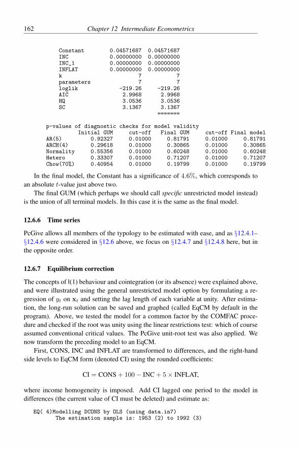
162 Chapter 12 Intermediate Econometrics
Constant 0.04571687 0.04571687INC 0.00000000 0.00000000INC_1 0.00000000 0.00000000INFLAT 0.00000000 0.00000000k 7 7parameters 7 7loglik -219.26 -219.26AIC 2.9968 2.9968HQ 3.0536 3.0536SC 3.1367 3.1367
=======
p-values of diagnostic checks for model validityInitial GUM cut-off Final GUM cut-off Final model
AR(5) 0.92327 0.01000 0.81791 0.01000 0.81791ARCH(4) 0.29618 0.01000 0.30865 0.01000 0.30865Normality 0.55356 0.01000 0.60248 0.01000 0.60248Hetero 0.33307 0.01000 0.71207 0.01000 0.71207Chow(70%) 0.40954 0.01000 0.19799 0.01000 0.19799
In the final model, the Constant has a significance of 4.6%, which corresponds toan absolute t-value just above two.
The final GUM (which perhaps we should call specific unrestricted model instead)is the union of all terminal models. In this case it is the same as the final model.
12.6.6 Time series
PcGive allows all members of the typology to be estimated with ease, and as §12.4.1–§12.4.6 were considered in §12.6 above, we focus on §12.4.7 and §12.4.8 here, but inthe opposite order.
12.6.7 Equilibrium correction
The concepts of I(1) behaviour and cointegration (or its absence) were explained above,and were illustrated using the general unrestricted model option by formulating a re-gression of yt on xt and setting the lag length of each variable at unity. After estima-tion, the long-run solution can be saved and graphed (called EqCM by default in theprogram). Above, we tested the model for a common factor by the COMFAC proce-dure and checked if the root was unity using the linear restrictions test: which of courseassumed conventional critical values. The PcGive unit-root test was also applied. Wenow transform the preceding model to an EqCM.
First, CONS, INC and INFLAT are transformed to differences, and the right-handside levels to EqCM form (denoted CI) using the rounded coefficients:
CI = CONS + 100− INC + 5× INFLAT,
where income homogeneity is imposed. Add CI lagged one period to the model indifferences (the current value of CI must be deleted) and estimate as:
EQ( 4)Modelling DCONS by OLS (using data.in7)The estimation sample is: 1953 (2) to 1992 (3)

12.6 Multiple regression 163
Coefficient Std.Error t-value t-prob Part.R^2Constant 18.1489 1.726 10.5 0.000 0.4180DINC 0.489427 0.02704 18.1 0.000 0.6802DINFLAT -0.709203 0.1826 -3.88 0.000 0.0892CI_1 -0.195899 0.01848 -10.6 0.000 0.4218
sigma 1.0962 RSS 185.054987R^2 0.758689 F(3,154) = 161.4 [0.000]**Adj.R^2 0.753988 log-likelihood -236.679no. of observations 158 no. of parameters 4mean(DCONS) -0.213409 se(DCONS) 2.2101
The outcome is a restricted, I(0), version of the ADL model, and all the coefficientestimates are well determined. The s value confirms that the restrictions are acceptable.Testing using the test summary yields:
AR 1-5 test: F(5,149) = 1.4037 [0.2262]ARCH 1-4 test: F(4,150) = 1.3152 [0.2669]Normality test: Chi^2(2) = 0.17211 [0.9175]Hetero test: F(6,151) = 0.55048 [0.7690]Hetero-X test: F(9,148) = 0.79076 [0.6253]RESET23 test: F(2,152) = 0.93003 [0.3968]
Thus, there is no evidence of mis-specification against the historical sample informa-tion. Figure 12.3 shows the goodness of fit and graphical statistics: we have added aregression line to the cross plot both to show its 45o angle, and to remind you that thesegraphs can be modified as flexibly as desired.
This concludes the EqCM analysis, except that the static regression in the next sec-tion both illustrates the Engle and Granger (1987) approach of OLS estimation of acointegrating model (but see Banerjee, Dolado, Hendry, and Smith, 1986), and showsthe effects of ‘correcting for residual autocorrelation’.
12.6.8 Non-linear least squares, COMFAC, and RALS
As an alternative to direct estimation of the EqCM, return to the general model in§12.6.4 (formulate a model, recall), but delete all the lagged variables, and estimatethe resulting static regression (from 1953(2)). If the variables were I(1), this might bethe first step of the Engle-Granger procedure.
EQ( 5) Modelling CONS by OLS (using data.in7)The estimation sample is: 1953 (2) to 1992 (3)
Coefficient Std.Error t-value t-prob Part.R^2Constant -147.330 22.00 -6.70 0.000 0.2244INC 1.15256 0.02462 46.8 0.000 0.9340INFLAT -2.47521 0.2051 -12.1 0.000 0.4845
sigma 3.27725 RSS 1664.75407R^2 0.942098 F(2,155) = 1261 [0.000]**Adj.R^2 0.941351 log-likelihood -410.224no. of observations 158 no. of parameters 3mean(CONS) 875.848 se(CONS) 13.5326

164 Chapter 12 Intermediate Econometrics
Fitted DCONS
1960 1970 1980 1990-5
0
5 Fitted DCONS DCONS × Fitted
-5.0 -2.5 0.0 2.5 5.0
-5
0
5DCONS × Fitted
Residual
1960 1970 1980 1990
-2
0
2Residual DCONS
0 5 10
0
1 CorrelogramDCONS
Residual
-3 -2 -1 0 1 2 3
0.2
0.4
DensityResidual Residual
-3 -2 -1 0 1 2 3
-2.5
0.0
2.5
5.0 DistributionResidual
Figure 12.3 Goodness-of-fit measures for EqCM
RALS denotes rth-order autoregressive least squares, and is for estimating equa-tions with valid common factors, so that their dynamics can be appropriately simplifiedto an autoregressive error. The residual sum of squares function for RALS is non-linearin the parameters, so an analytic formula for the optimum does not exist, although nu-merical methods can be used to locate it. In fact, one could always use numerical meth-ods, even for OLS where an exact form does exist, although it might be a little slow. Toillustrate this principle, we first re-fit the static OLS regression by numerical optimiza-tion, and compare the outcome with the result found by the analytical formula. Accessthe Nonlinear modelling choice on the Model menu, and formulate the instructions asfollows:
actual = CONS;fitted = &0 + &1*INC + &2*INFLAT;&0 = -147.3301;&1 = 1.152563;&2 = -2.475206;
Estimate from 1953 (2); convergence is fast and the outcomes are almost identical (eventhough standard errors are calculated numerically, not from the variance formula): inparticular, the RSS values match precisely.
EQ( 6) Modelling actual by NLS (using data.in7)The estimation sample is: 1953 (2) to 1992 (3)
Coefficient Std.Error t-value t-prob Part.R^2&0 -147.33 22.00 -6.70 0.000 0.2244&1 1.1526 0.02462 46.8 0.000 0.9340

12.6 Multiple regression 165
&2 -2.4752 0.2051 -12.1 0.000 0.4845
sigma 3.27725 RSS 1664.75407R^2 0.942098 F(2,155) = 1261 [0.000]**no. of observations 158 no. of parameters 3
Standard errors based on information matrixBFGS/warm-up using numerical derivatives (eps1=0.0001; eps2=0.005):Strong convergence
Following the route at the end of the previous section, for the static model of CONSon INC and INFLAT, the value of the DW statistic suggests a high degree of residualautocorrelation. This ‘problem’ might be ‘corrected’ by removing the autocorrelation,so we consider that possibility next. Recall the static model, and estimate from 1953(2)using Autoregressive Least Squares (RALS), with a first-order error process. At theRALS estimation dialog, use Grid to graph the log-likelihood as a function of the first-order autoregressive error parameter.11 Multiple optima are quite common in RALS,and can be revealed by this procedure. Here, you will find that the optimum is onthe boundary at unity – not an auspicious start. Use Estimate to start the numericaloptimization, and OK to conclude.
EQ( 7) Modelling CONS by RALS (using data.in7)The estimation sample is: 1953 (2) to 1992 (3)
Coefficient Std.Error t-value t-prob Part.R^2Constant 403.491 34.87 11.6 0.000 0.4651INC 0.519878 0.03548 14.7 0.000 0.5823INFLAT -0.724649 0.2449 -2.96 0.004 0.0538Uhat_1 0.988354 0.01450 68.2 0.000 0.9679
sigma 1.43855 RSS 318.693176no. of observations 158 no. of parameters 4
NLS estimation using analytical derivatives (eps1=0.0001; eps2=0.005):Strong convergenceRoots of error polynomial:
real imag modulus0.98835 0.00000 0.98835
Consider these results in the light of §12.4.7, and use the RSS value to calculatea likelihood ratio test of COMFAC against the unrestricted dynamic model in §12.6(RSScomfac(4) = 318.69 and RSSunrest(6) = 176.75):
FK1−K2
T−K1=
(318.69− 176.75)× 152
176.75× 2= 61.
The evidence fits like a glove: the DGP is not COMFAC, but EqCM. Figure 12.4 showsthe RALS graphical output.
11This is the concentrated (or profile) likelihood: for each autoregressive value the likelihoodis maximized.

166 Chapter 12 Intermediate Econometrics
Fitted CONS
1960 1970 1980 1990
860
880
900Fitted CONS CONS × Fitted
860 870 880 890
860
880
900CONS × Fitted
Residual
1960 1970 1980 1990
-2.5
0.0
2.5 Residual CONS
0 5 10
0
1 CorrelogramCONS
Residual
-4 -3 -2 -1 0 1 2 3
0.2
0.4
DensityResidual Residual
-4 -3 -2 -1 0 1 2 3
-2.5
0.0
2.5
5.0 DistributionResidual
Figure 12.4 Goodness-of-fit measures for RALS
12.7 Econometrics concepts
12.7.1 Innovations and white noise
It is possible to obtain a significant value on a COMFAC test, yet the residuals of theresulting RALS model be white noise according to the residual correlogram (Portman-teau) statistic; such an outcome illustrates a non-innovation white-noise process. Theformer outcome (i.e., COMFAC rejects) entails that a better model can be developed onthe same information set (that is, a model which does not impose COMFAC) – so theerror is not an innovation. The latter outcome shows that the same error is white noise(not serially correlated).
An alternative illustration of that distinction can be created by dropping the EqCMterm from the model in §12.6. The correlogram statistic can be insignificant, but theomitted-variable test option shows that the EqCM term still matters, so that the resid-uals are not an innovation against lagged levels information (see Davidson, Hendry,Srba, and Yeo, 1978, and Hendry and von Ungern-Sternberg, 1981, for empirical ex-amples). Delete the equilibrium-correction term from the model in §12.6.7, and add inthe 1-period lags of the three differences (so the resulting model has no long-run levelssolution) to produce:
EQ( 8) Modelling DCONS by OLS (using data.in7)The estimation sample is: 1953 (3) to 1992 (3)
Coefficient Std.Error t-value t-prob Part.R^2DCONS_1 0.260429 0.07369 3.53 0.001 0.0764Constant -0.0644508 0.1042 -0.619 0.537 0.0025

12.7 Econometrics concepts 167
DINC 0.527350 0.03262 16.2 0.000 0.6338DINFLAT -0.529530 0.2883 -1.84 0.068 0.0218DINC_1 -0.00786886 0.04963 -0.159 0.874 0.0002DINFLAT_1 -0.744058 0.2822 -2.64 0.009 0.0440
sigma 1.29654 RSS 253.831609R^2 0.662972 F(5,151) = 59.41 [0.000]**no. of observations 157 no. of parameters 6
Figure 12.5 reports the corresponding graphical information: the correlogram is fairlyflat and close to that of a white-noise process even though the errors contain the omittedEqCM, which would have a t-value of about 10 if entered directly in the model. Anappropriate test for autocorrelated errors would reject, however. Also see the discussionin Hendry (1995a), and in §15.2 and §15.3.
Fitted DCONS
1960 1970 1980 1990
-5
0
5Fitted DCONS DCONS × Fitted
-4 -2 0 2 4
-5
0
5DCONS × Fitted
Residual
1960 1970 1980 1990-2.5
0.0
2.5 Residual DCONS
0 5 10
0
1 CorrelogramDCONS
Residual
-3 -2 -1 0 1 2 3 4
0.2
0.4
DensityResidual Residual
-3 -2 -1 0 1 2 3 4
-2.5
0.0
2.5
5.0 DistributionResidual
Figure 12.5 Mis-specified EqCM with near white-noise residuals
12.7.2 Exogeneity
This analytic notion is described in §14.7.2, and recurs in §15.5: for a fuller treatmentsee Engle, Hendry, and Richard (1983). To illustrate, it happens that, in the presentdata set, there is no valid consumption function with income weakly exogenous forinvariant parameters of interest (CONS and INC are simultaneously determined); thisis not easily tested at an intermediate level: however, instrumental variables methods(discussed below) could be used to investigate such a difficulty.
The comparison of §12.5.3 and §12.5.4 is illuminating since xt is not weakly ex-ogenous for β in the latter. The required exogeneity condition is that β can be learned

168 Chapter 12 Intermediate Econometrics
from the conditional model alone, without loss of information. Thus, the xt variablescan be taken as given, or ‘determined outside the model under consideration’. That thiscondition fails here is clear from the construction of the DGP in the Appendix. It alsofollows on the ‘conventional’ notion of exogeneity, since E [xtεt] 6= 0 in §12.5.4. Nev-ertheless, the ‘conventional’ notion of exogeneity is flawed, as we now explain. Whenthe DGP is stationary, regressing yt on xt will deliver a coefficient vector α (say) withthe property that E [yt|xt] = α′xt, and so there exists a model yt = α′xt + ξt whereE [xtξt] = 0. Apparently, xt is now ‘exogenous’! Indeed, xt is weakly exogenousfor α in that model, but α is, of course, not the parameter of interest, β. However,the two parameters are related, which we illustrate by letting xt = Γxt−1 + νt, soE [xt|xt−1] = Γxt−1, and E [νtν
′t] = Ω. In §12.5.4, we saw that E [νtηs] = 0 ∀t, s
was not sufficient for xt to be weakly exogenous for β. Under stationarity, lettingΦ = E [xtx
′t], then:
α = (E [xtx′t])−1
(E [xtyt]) =(Ik −Φ−1Ω
)β,
and so depends on Γ and Ω. Thus, β cannot be obtained from α without knowledge of(Γ, Ω), which are the parameters of the xt process, showing that the requirementsfor weak exogeneity are not satisfied: the parameter of interest can be obtained onlyby modelling xt. This case is most easily derived for a scalar x-process, whereΦ = Ω/
(1− Γ2
)and α = Γ2β. This outcome is closely related to errors-in-variables
models, such as permanent income.Finally, the presence or absence of xt in the equation is not germane to its weak
exogeneity status. To show that, §12.5.4 entails that yt = β′Γxt−1 + εt + β′νt andhence E [yt|xt−1] = β′Γxt−1 is a valid specification for regression. However, β canbe obtained from β′Γ only if Γ is known, which necessitates estimating the marginalmodel for xt. That example reveals that xt need not be weakly exogenous for theparameter of interest even when xt is absent from the equation analyzed.
Importantly, non-stationarity is the more usual state for economic time series, inwhich case Γ and Ω are likely to be non-constant, inducing non-constancy in α evenwhen β is constant. Thus, we turn to investigating that issue.
12.7.3 Constancy and invariance
Recursive-estimation techniques are discussed formally in Chapter 13, but PcGive em-bodies graphical options which make parameter constancy, or its absence, easy to illus-trate. The basic idea is straightforward. A tedious way to see if parameters are constantwould be to fit the model to the first M > k observations for k parameters, then tofit it to M + 1, M + 2 etc. up to T , yielding T −M + 1 estimates of each coeffi-cient and its standard error over the sample. Plotting these would reveal any changesrelative to the standard error measures. Fortunately, there are clever ways of doing sobuilt into PcGive and we merely have to choose recursive estimation to obtain all therequired statistics and associated tests. Use the same model as the final one for DCONSin §12.6.7, and estimate by RLS. Figure 12.6 illustrates the graphical output.

12.7 Econometrics concepts 169
Constant
1960 1970 1980 1990
10
20
30Constant DINC
1960 1970 1980 1990
0.4
0.6
0.8DINC
DINFLAT
1960 1970 1980 1990-2
-1
0DINFLAT CI_1
1960 1970 1980 1990
-0.3
-0.2
-0.1
0.0CI_1
Res1Step
1960 1970 1980 1990-2.5
0.0
2.5 Res1Step
Ndn CHOWs 1%
1960 1970 1980 1990
0.5
1.0
Ndn CHOWs 1%
Figure 12.6 Recursive constancy statistics for EqCM
The first four plots are of the coefficient estimates at each point in the sample to-gether with their approximate 95% confidence intervals (±2SE shown on either side);for most of the data set, the estimates are significantly different from zero, and are rel-atively constant over the sample once past the initial estimation. The fifth plot is ofthe 1-step ahead residuals (forecast errors) also with an approximate 95% confidenceinterval; the confidence bands are again reasonably constant, but increase somewhataround 1974. However, the final plot of the break-point Chow test (see Chow, 1960)shows that constancy is rejected at the 1% level over the oil-crisis period, and lookingmore carefully at the coefficient plots, the change in the coefficient of DINFLAT isnoticeable.
Invariance is more complex to illustrate, so the artificial data set is helpful. (TheAppendix shows the DGP for the tutorial data set.) Consider a sine wave – it is non-constant, but invariant to other changes. Above, we found that α was constant understationarity, but not invariant to changes in the process generating x. Thus, the twoconcepts are distinct. To test for invariance in a regression model, one must first findchanges in the processes generating the regressors, then check if any regression param-eters shift at the same time: that would refute a claim of invariance. Here, a modelof INFLAT on OUTPUT and INFLAT 1 is highly non-constant following 1973(3) (seeFigure 12.7). This is precisely the point at which the coefficient of DINFLAT showeda shift in the conditional EqCM model, EQ(4), consistent with non-invariance of theinflation coefficient: see the last panel Figure 12.7. The common omitted factor in bothmodels is the Oil-price jump. A more realistic case of invariance analysis is describedin Hendry (1988).

170 Chapter 12 Intermediate Econometrics
INFLAT_1 × +/-2SE
1960 1970 1980 1990
0.8
1.0
INFLAT_1 × +/-2SE Constant × +/-2SE
1960 1970 1980 1990
-100
-50
0 Constant × +/-2SE
OUTPUT × +/-2SE
1960 1970 1980 19900.00
0.05
0.10 OUTPUT × +/-2SE Res1Step
1960 1970 1980 1990
0
1Res1Step
Ndn CHOWs 1%
1960 1970 1980 1990
1
2Ndn CHOWs 1% DINFLAT × +/-2SE from EQ(4)
1960 1970 1980 1990-2
0
2DINFLAT × +/-2SE from EQ(4)
Figure 12.7 Recursive constancy statistics for marginal, and invariance comparison
12.7.4 Congruent models
We have now seen a variety of criteria that a model might reasonably be required tosatisfy, such as white-noise, innovation errors, homoscedasticity, constant parametersthat appear invariant to important historical and policy changes, and weakly exogenousconditioning variables for the parameters of interest. The first three relate to the abil-ity of a model to characterize the past; the middle two, to its ability to describe thefuture; and the last to its validity in the present. A model which shows no departuresfrom the data on any of the evaluation criteria is said to be congruent with the evidence.Non-congruent models can always be dominated by a model that explains the previousmis-match; and the DGP is clearly congruent with the data, so congruent models havemuch to recommend them. However, a sequence of congruent models of any given phe-nomenon could be developed, each explaining more by augmenting the information setappropriately. Thus, we need a further criterion to choose between them, as discussedin the next section.
12.7.5 Encompassing rival models
Encompassing is easy to illustrate in PcGive, so we first explain the concept and itsproperties. Consider two rival explanations of a given variable denoted by M1 and M2.The question at issue is whether the M2 model can explain features of the data whichthe M1 model cannot. This is a test of M1, with M2 providing the alternative, to seewhether M2 captures any specific information not embodied in M1. The converse iswhether M1 can account for all the results found by M2, and that idea is formalized

12.7 Econometrics concepts 171
in the notion of encompassing (see Hendry and Richard; Hendry and Richard, 1982,1989, Mizon, 1984, and Mizon and Richard, 1986). A congruent undominated modelshould encompass (that is, account for) previous empirical findings claimed to explainthe given dependent variable(s). Encompassing is denoted by E so if the relevant mod-els are M1 and M2, then M1 EM2 reads as ‘M1 encompasses M2’. Notice that variancedominance (fitting better on the basis of error variance) is not sufficient for encompass-ing (the other model could still explain part of what the first did not), but is necessary(as the better-fitting model clearly explains some aspects better than the other).
The ease of handling general models allows embedding approaches to be almostautomatic in PcGive. Encompassing and non-nested hypothesis tests are offered forOLS and instrumental variables (IV), based on Cox (1961), Pesaran (1974) and Eric-sson (1983), allowing pairs of single equation models to be tested directly. As arguedin Hendry and Richard (1989), encompassing essentially requires a simple model toexplain a more general one within which it is nested (often the union of the simplemodel with its rivals); this notion is called parsimonious encompassing and is denotedby Ep. An important property of parsimonious encompassing is that it defines a partialordering over models, since Ep is transitive, reflexive, and anti-symmetric. Since someaspects of inference must go wrong when a model is non-congruent, encompassing testsshould only be conducted with respect to a ‘baseline’ congruent model; and is anywayunnecessary otherwise since non-congruence already demonstrates inadequacies (for aformal analysis, see Bontemps and Mizon, 2003).
To apply encompassing procedures, we need to have two non-nested models ofinterest. For the first, use the ADL (1 lag) of CONS on INC and INFLAT; and for thesecond CONS on OUTPUT with two lags of each, both from 1953(3). Formulate andestimate them in that order, then from the Test menu, select Encompassing to produce:
Encompassing test statistics: 1953 (3) to 1992 (3)
M1 is: CONS onConstant CONS_1 INC INC_1 INFLAT INFLAT_1
M2 is: CONS onCONS_1 CONS_2 Constant OUTPUT OUTPUT_1 OUTPUT_2
Instruments used:Constant CONS_1 INC INC_1 INFLATINFLAT_1 CONS_2 OUTPUT OUTPUT_1 OUTPUT_2
sigma[M1] = 1.08126 sigma[M2] = 2.03616 sigma[Joint] = 1.09367
Test Model 1 vs. Model 2 Model 2 vs. Model 1Cox N(0,1) = 0.1961 [0.8445] N(0,1) = -46.16 [0.0000]**Ericsson IV N(0,1) = -0.1929 [0.8471] N(0,1) = 24.69 [0.0000]**Sargan Chi^2(4) = 0.60786 [0.9622] Chi^2(4) = 108.59 [0.0000]**Joint Model F(4,147) = 0.14861 [0.9634] F(4,147) = 94.099 [0.0000]**
The tests produced are those due to Cox (1961), (distributed asymptotically as N[0, 1]
on the null of encompassing; Ericsson (1983) (an IV-based test with the same limitingdistribution), another IV test developed by Sargan (1959), distributed as χ2 with thedegrees of freedom shown, and the F-test for each model being a valid simplification of

172 Chapter 12 Intermediate Econometrics
the linear union of the two models under test. The second model clearly does not en-compass the first on any of the tests, whereas the first is not rejected by the second. Weconclude that the second is inferentially redundant and the first remains undominated.Since empirical models can be designed to satisfy a range of criteria (see §12.10), en-compassing tests against models designed by other investigators offer a useful checkagainst spurious findings.
12.8 Instrumental variablesThe method of instrumental variables was developed to handle endogenous regressorsin models, but using limited information. It may happen that in the linear equation(12.28), E [yt|xt] 6= x′tβ so that E [xtεt] 6= 0. An example is a behavioural model.Then OLS estimation is not consistent for β (try proving this claim). Assume there is ak × 1 vector zt such that:
E [yt | zt] = E [xt | zt]′ β (12.34)
so E [z′tεt] = 0. The role of zt is purely instrumental in estimating β, and its use leads toinstrumental variables estimators (IVE) as follows (the case of more than k instrumentsis handled automatically by PcGive, but β is not estimable when there are fewer than kinstruments).
We only consider the case where E [Z′ε] = 0 but in y = Xβ + ε, E [X′ε] 6= 0.Premultiply (12.29) by Z′:
Z′y = Z′Xβ + Z′ε (12.35)
When rank(T−1Z′X
)= k, so that the matrix is invertible (which is also sufficient to
identify β: see White, 1984) then rank(T−1Z′Z
)= k. Thus, setting Z′ε = 0,,which it
should be on average:β = (Z′X)
−1Z′y (12.36)
which is the instrumental variables estimator. In large samples, its variance matrix isestimated by:
σ2ε
[X′Z (Z′Z)
−1Z′X
]−1
(12.37)
where:
ε = y −Xβ and σ2ε =
ε′ε
T − k. (12.38)
Check that the formulae collapse to the OLS outcomes when Z = X. However, statis-tics like R2 are not so easily defined.
The fourth case of §12.5 can be compared to the third when the IVs are vari-ables in It−1. When §12.5.3 holds with εt being an innovation against It−1, thenE [yt|xt] = x′tβ implies that E [yt|It−1] = β′E [xt|It−1] also. The converse does nothold, however, otherwise types §12.5.3 and §12.5.4 would coincide. Check that you canprove this claim. Since the failure of OLS is owing to the xt process being informa-tive about the parameter of interest, the analysis of exogeneity above is directly relevantto clarifying when regression can be used.

12.9 Inference and diagnostic testing 173
The EqCM model of CONS in fact has INC endogenous owing to contemporaneousfeedback, so we now estimate it by IV, using 1-lagged values of DCONS and DINC asinstruments, as well as the other regressors (DINFLAT and the CI 1). The full sampleestimates and test statistics are:
EQ( 9) Modelling DCONS by IVE (using data.in7)The estimation sample is: 1953 (3) to 1992 (3)
Coefficient Std.Error t-value t-probDINC Y 0.440453 0.1323 3.33 0.001Constant 18.5348 1.884 9.84 0.000DINFLAT -0.618109 0.2714 -2.28 0.024CI_1 -0.200159 0.02026 -9.88 0.000
sigma 1.11086 RSS 188.804732Reduced form sigma 1.9202no. of observations 157 no. of parameters 4no. endogenous variables 2 no. of instruments 5
Additional instruments:[0] = DCONS_1[1] = DINC_1
Specification test: Chi^2(1) = 0.5315 [0.4660]Testing beta = 0: Chi^2(3) = 155.66 [0.0000]**
As can be seen by comparing with the earlier OLS results, the coefficients of INC andINFLAT are smaller, and their standard errors much larger. The EqCM coefficient issomewhat larger. The value of s is not much altered, but the much larger value of the‘reduced form’ s (which measures the fit from regressing CONS on the instruments)shows the importance of contemporaneous information. The specification χ2 tests forthe independence of the instruments and the errors (see §17.3.3 and Sargan, 1958) doesnot reject, and the diagnostic tests yield similar outcomes to OLS. We conclude thissection with the recursive statistics graphs (no equivalent of the Chow tests is providedfor IV) shown in Figure 12.8. The parameters are reasonably constant, although thatfor INFLAT still shows signs of changing around the oil crisis.
12.9 Inference and diagnostic testingMany aspects of inference and testing have occurred above, so a preliminary knowl-edge was implicitly assumed throughout. Formal derivations will not be presented (seeGodfrey, 1988) but the intuition behind the Lagrange Multiplier (LM)-test for residualautocorrelation, ARCH etc. is useful. These statistics are essentially extrapolating fromthe likelihood function value when a parameter has been restricted (usually to zero) towhat the likelihood value would be when the parameter was estimated. When the like-lihood is quadratic, the score is linear and the extrapolation is completely successful(that is, the outcome is the same as a likelihood-ratio test). Asymptotically, as likeli-hoods are quadratic, LM-tests become fully powerful for the correct size (null rejectionfrequency).
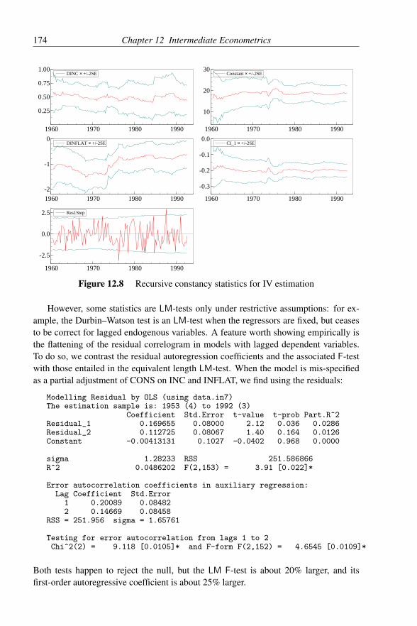
174 Chapter 12 Intermediate Econometrics
DINC × +/-2SE
1960 1970 1980 1990
0.25
0.50
0.75
1.00DINC × +/-2SE Constant × +/-2SE
1960 1970 1980 1990
10
20
30Constant × +/-2SE
DINFLAT × +/-2SE
1960 1970 1980 1990
-2
-1
0DINFLAT × +/-2SE CI_1 × +/-2SE
1960 1970 1980 1990
-0.3
-0.2
-0.1
0.0CI_1 × +/-2SE
Res1Step
1960 1970 1980 1990
-2.5
0.0
2.5 Res1Step
Figure 12.8 Recursive constancy statistics for IV estimation
However, some statistics are LM-tests only under restrictive assumptions: for ex-ample, the Durbin–Watson test is an LM-test when the regressors are fixed, but ceasesto be correct for lagged endogenous variables. A feature worth showing empirically isthe flattening of the residual correlogram in models with lagged dependent variables.To do so, we contrast the residual autoregression coefficients and the associated F-testwith those entailed in the equivalent length LM-test. When the model is mis-specifiedas a partial adjustment of CONS on INC and INFLAT, we find using the residuals:
Modelling Residual by OLS (using data.in7)The estimation sample is: 1953 (4) to 1992 (3)
Coefficient Std.Error t-value t-prob Part.R^2Residual_1 0.169655 0.08000 2.12 0.036 0.0286Residual_2 0.112725 0.08067 1.40 0.164 0.0126Constant -0.00413131 0.1027 -0.0402 0.968 0.0000
sigma 1.28233 RSS 251.586866R^2 0.0486202 F(2,153) = 3.91 [0.022]*
Error autocorrelation coefficients in auxiliary regression:Lag Coefficient Std.Error
1 0.20089 0.084822 0.14669 0.08458
RSS = 251.956 sigma = 1.65761
Testing for error autocorrelation from lags 1 to 2Chi^2(2) = 9.118 [0.0105]* and F-form F(2,152) = 4.6545 [0.0109]*
Both tests happen to reject the null, but the LM F-test is about 20% larger, and itsfirst-order autoregressive coefficient is about 25% larger.

12.10 Model selection 175
A similar bias occurs even if there is no lagged dependent variable, but xt isGranger-caused by y (see Granger, 1969, and Hendry and Mizon, 1999): again thisis easy to demonstrate. Many other tests can be computed using PcGive, but in general,inference is better illustrated using Monte Carlo to simulate the actual distributions,sizes and powers. Nevertheless, the methodology of modelling is open to analysis atthis stage, of which mis-specification tests are one aspect, so we turn to consider that.
12.10 Model selectionSome discussion, and empirical illustration, of the issue of model selection is imperativeif econometrics is to find any practical use, even as a set of critical skills. Unfortunately,the topic is a vast one, often misunderstood (and subject to folklore, rather than fact),and so prone to disastrous outcomes in a teaching context. Nevertheless, we will firstdescribe a general framework, then consider model design.
12.10.1 Three levels of knowledge
It is useful to distinguish between the three levels of knowledge potentially available ina theoretical analysis. Write the data set as X1
T = (x1 . . .xT ) and denote the DGP bythe joint data density DX
(X1T |θ). Then:
1. Both DX (·) and θ being known corresponds to a probability theory course: that is,given DX (·|θ), what xs will be observed, and with what probabilities of lying invarious regions? The analyses in the first two sections above are examples of thislevel of knowledge.
2. DX (·) known and θ unknown corresponds to an estimation and inference course,that is, given X1
T and knowledge of DX (·), how should one estimate θ? This routeleads on to likelihood, maximum likelihood estimation etc., and characterizes thestate of knowledge implicit in Chapter 13.
3. Both DX (·) and θ unknown corresponds to a modelling course: that is, given onlyX1T how do we discover, design or develop useful models of the observables, and
what criteria characterize ‘useful’ etc.?Since (3) is the realistic situation in empirical econometrics, §12.6 discussed a num-
ber of the background issues. The illustrations above fell in an intermediate state, as weknew the DGP, but did not use that knowledge except to explain the observed outcomes– and the reader did not necessarily know the DGP.
Two important issues arise once the limited knowledge of (3) is granted: first, thepostulated likelihood function for an empirical model need not coincide with the actualdensity function of the observables; and secondly, models will inevitably be simpli-fications, not facsimiles of the economic mechanism. Both issues highlight that it iscrucial to test empirical claims rigorously – and that feature is certainly built into Pc-Give. More fundamentally, we must first address the selection of the criteria by whichto judge models, and the problems deriving from our ability to design empirical modelsto achieve such pre-specified criteria, even when the DGP does not satisfying those cri-

176 Chapter 12 Intermediate Econometrics
teria. The former was briefly addressed above in the context of congruency, so we turnto the latter.
12.10.2 Modelling criteria
Sections 14.5 and 14.7 will consider more rigorously the range of relevant criteria formodel selection in terms of necessary conditions for congruence. As noted earlier, amodel is congruent when it matches the available evidence in all the dimensions exam-ined (for example, has innovation, homoscedastic errors, constant parameters etc.). Tocheck whether or not a model does match the evidence is a ‘destructive’ application ofinference (testing in order to reject), and that destructive, or evaluation, aspect has beencovered (in part) already in §12.6 above (see Baba, Hendry, and Starr, 1992, for an ex-ample analyzing US M1 demand). We now seek more constructive criteria, always withthe caveat that corroboration is not definitive (see e.g. Ericsson and Hendry, 1999).
Information criteria, which penalize for additional parameters more just than thedegrees of freedom adjustment to σ, are often used – but assume that many of thenecessary criteria for congruence are already satisfied. They are related to the use ofR2, R2 and σ2 as model-selection criteria, and in finite samples seem preferable tothose. PcGive provides three, namely the Schwarz, Hannan–Quinn, and final predictionerror criteria (see Chapter 17), and uses the Schwarz criterion in general-to-specificmodelling for selecting between congruent simplifications. However, within a classof models under comparison, nothing justifies the ‘best’ of these by any informationcriterion when they are all badly mis-specified – which emphasizes the prior need tohave established the ‘goodness’ of the class as a data description. Thus, we come backto the need to develop congruent models, then select between these by encompassing.
That approach involves two stages: first formulate and test the general model; thensimplify it to a parsimonious, undominated relation (model reduction). The first step iswhen we use mis-specification tests to evaluate the congruence of the general model;the use of diagnostic tests at later stages (during simplification) is merely as an aidto revealing invalid reductions. The statistical problems concern the probabilities ofthe mis-specification tests (which is relatively easy in technical terms, and could beresolved by a single ‘portmanteau’ test), and the consequences of ‘revising the modelin the light of test rejections’. The latter is only amenable to general discussion, since ifthe revision chanced to lead to specifying the DGP, the consequences would be brilliant– but that seems unlikely. Thus, we next consider the problem of ‘covert’, or implicit,design of models specifically to render insignificant any mis-specification tests.
12.10.3 Implicit model design
The reinterpretation of RALS estimation, following a significant residual autocorrela-tion test, as covert, or implicit, design should now be clear. Irrespective of the causeof the residual autocorrelation, a high enough order autoregressive error process fittedto the residuals can remove residual autocorrelation – and hence ‘designs’ the modelaccording to a white-noise selection criterion. In the discussion of COMFAC, we noted

12.10 Model selection 177
that the order of hypothesis testing was incorrect. One must first establish the congru-ence of the general dynamic relation, then test for common factors in the dynamics,and finally test their significance when they the provide a valid reduction. More gener-ally, we saw the problems with unstructured searches such as simple-to-general at thestart of this chapter. A simple model of a complicated process can be made to ‘work’by selecting a particular criterion (for example, white-noise residuals) and an associ-ated test statistic, then successively correcting the problem until the test is insignificant.However, a second test (for example, COMFAC, or constancy) may still reject, forcingthe entire exercise up to that point to be discarded, or lead to an unfounded strategy ofpatching the next mistake. Rejection means that all previous inferences were invalid,including even the existence of the initial problem. Thus, simple-to-general is an inef-ficient research strategy. Apparent residual autocorrelation (say) could derive from thewrong functional form (linear instead of log), or even parameter change: ‘fixing’ resid-ual autocorrelation is then valueless. Also, alternative routes begin to multiply becausesimple-to-general is a divergent branching process – there are many possible solutionsto each rejection, but the model evolves differently depending on which is selected, andin what order. Moreover, when should you stop testing or correcting previous rejec-tions? There are obvious dangers in stopping at the first non-rejection (see the analysisof selecting the order of an autoregressive process in Anderson, 1971).
Conversely, with a pre-defined stopping point (that is, a general model in the back-ground), a more coherent strategy is possible. The ordering of hypothesis tests is oftenclearer, rejections do not lead to a loss of previous work, and the tests are nested. Oncethe initial general model is rigorously tested for congruence, later tests are of reduc-tions, not of model validity. Further, it is clear when to stop: when the selected modelparsimoniously encompasses the initial general model, but fails to do so on further sim-plification. Of course, if the initial model is non-congruent, there is no alternative toa generalization, but that is not a telling argument against general-to-simple (denotedGets below): a simpler starting point would fare even less well.
12.10.4 Explicit model design
Consequently, PcGive is easiest to use for sequential simplification following the test-ing for congruence of the initial general model (often called the statistical model: seeSpanos, 1986). Why simplify? We consider that parsimony is essential for test powerand for interpretability, and is often found to sustain parameter constancy. Collinearityis not the driving force behind simplification: we saw above that models can be de-signed to have orthogonal parameters, however many regressors there are. On the otherhand, orthogonality is useful for robustness and for testing for the marginal significanceof each variable in isolation (that is, without strong ceteris paribus assumptions), aswell as for interpretability. Thus, we aim to conclude with parsimonious models whichhave orthogonal regressors, as well as satisfying the necessary conditions for both con-gruence and encompassing.
Models can also be designed to be consistent with the available economic theory,which leads to the concept of an econometric model (which again must be congruent

178 Chapter 12 Intermediate Econometrics
and should parsimoniously encompass the statistical model). Section 14.7.7 discussessequential simplification in the theory of reduction (the Progress menu tracks explicitdesigns). Although it may seem to be useful to retain a subset of data throughout (forexample, by initially loading only a time subset of the available data), since Neyman–Pearson testing for quality control can then be undertaken at the end of the analysis,what would you do next if this led to rejection after six months’ work?
The process of model simplification can be surprisingly time consuming, so we havedeveloped an automated procedure called Autometrics, see Doornik (2009), Doornik(2008). This follows on from Hendry and Krolzig (1999) and Hoover and Perez (1999).There is now considerable Monte Carlo simulation evidence that Gets performs well,selecting a model from an initial general specification almost as often as the same cri-teria would when applied to the DGP (since test size leads to false rejections, and non-unit power to false acceptances of the null even when the analysis commences from the‘truth’). Chapter 14 discusses this in more detail.
A vast number of other aspects of model design could be illustrated, but we hopethat the flavour of econometric modelling is now both well established and has provedinteresting. Chapter 14 discusses the theory of reduction, model concepts, the informa-tion taxonomy, and modelling more formally, building on Hendry (1987). An overviewis presented in Hendry and Richard (1983), and Hendry (1993), Hendry (2000a) pro-vides a collection of papers on modelling methodology (see especially, Hendry, 2000b).Hendry and Doornik (1994) and Hendry, Neale, and Srba (1988) extend the analysis tolinear systems modelling, including recursive estimation of simultaneous systems andVARs. Hendry (1988) considers the refutability of the Lucas critique for models withcurrent-dated expectations variables using such techniques. On the rapidly developingsubject of cointegration, many of the currently proposed estimators and tests are easilycalculated (see Engle and Granger, 1987, and Phillips, 1987 among others). The Jo-hansen (1988) procedure is implemented in the system procedures discussed in VolumeII. Monte Carlo is also useful as an illustrative tool, given the difficulty of analyticalderivations of sampling distributions; but that is the subject of a separate program (seethe companion book on Ox as well as Hendry, Neale, and Ericsson, 1991).

Chapter 13
Statistical Theory
13.1 IntroductionWe will review three main statistical tools: regression, maximum likelihood, and leastsquares. To explain these closely related methods of estimating unknown parameters,we first introduce the normal distribution for one variable, then the bivariate normaldistribution, and finally a multivariate normal. A regression is a conditional relationand arises when looking at the conditional distribution of one random variable, denotedY , given values of another, denoted Z (capital letters here denote random variables,and lower case their realizations). In a bivariate normal, the regression is linear, so hasthe form E[Y |z] = α + βz when Z = z, which provides an introductory case. Ina multivariate normal, the regression remains linear, but involves several variables (k,say), denoted by a vector z = (z1 . . . zk)
′.Such regressions are defined in terms of unknown parameters, like α and β, and
these require estimation from sample data. When samples are randomly drawn from acommon population, and the linear regression holds for that population, then maximumlikelihood or least squares will deliver ‘good’ estimates in general. These methods aredescribed in §13.5 and §13.7.
13.2 Normal distribution
The normal, or Gaussian, density fx(x|µx, σ2
x
)of a random variable X is defined by:
fx(x | µx, σ2
x
)=(2πσ2
x
)− 12 exp
[− (x− µx)
2
2σ2x
](13.1)
where |µx| < ∞ and 0 < σ2x < ∞ for x ∈ R. The normal density function reaches
a maximum at x = µx and is symmetric about µx which is the mean: E[X] = µx.Its spread increases with σ2
x which is the variance: E[(X − µx)2] = σ2
x; the squareroot σx =
√σ2x is the standard deviation. The normal distribution is denoted by X ∼
179

180 Chapter 13 Statistical Theory
N[µx, σ
2x
], and read as: X is distributed as a normal random variable with mean µx
and variance σ2x.
Let Y = (X − µx) /σx so that X = σxY + µx. This linear transform from X toY alters the density to:
fy (y | ·) =(2πσ2
x
)− 12 exp
[− 1
2 y2]σx = (2π)
− 12 exp
[− 1
2 y2]. (13.2)
This is the standardized form of the density, denoted by Y ∼ N [0, 1]. Note that fx (x) ≥0 since the exponential function is always positive, and that the density integrates tounity: ∫ ∞
−∞(2π)
− 12 exp
[− 1
2 y2]
dy = 1.
13.3 The bivariate normal density
Consider two random variables denoted X and W . The correlation corr [X,W ] = ρ
between X and W is defined by:
ρ =E [(X − µx) (W − µw)]√
E[(X − µx)
2]
E[(W − µw)
2] =
σxwσxσw
where σxw is the covariance. It can be shown that −1 ≤ ρ ≤ 1. When X and W aredistributed according to a standardized bivariate normal distribution, the formula forfx,w (x,w | ρ) is:
fx,w (x,w | ρ) =(
2π√
(1− ρ2))−1
exp
[−(x2 − 2ρxw + w2
)2 (1− ρ2)
]. (13.3)
Since exp [·] has a non-positive argument, its value is positive but less than unity, andhence: (
2π√
(1− ρ2))−1
≥ fx,w (x,w) ≥ 0. (13.4)
For the standardized bivariate normal distribution, the covariance E[XW ] = σxw = ρ,and ρ = 0 is necessary and sufficient to ensure independence between X and W .
Linear combinations of jointly normal variables are also normal. The proof is basedon deriving the distribution of the random variables (aX + bW : W ) where (X : W )
is bivariate normal and a 6= 0.
13.3.1 Marginal and conditional normal distributions
The marginal distribution of W is normal, and from it we can obtain the conditionaldistribution of X given W denoted fx|w (x|w). By definition, the marginal density ofW is:
fw (w) =
∫ ∞−∞
fx,w (x,w) dx. (13.5)

13.3 The bivariate normal density 181
Calculating that expression for the standardized bivariate normal yields:∫ ∞−∞
(2π√
(1− ρ2))−1
exp
[−(x2 − 2ρxw + w2
)2 (1− ρ2)
]dx. (13.6)
The term in [·] can be rewritten as[(x− ρw)
2+(1− ρ2
)w2]
(a result of use below).
Since exp (a+ b) = exp (a) exp (b), then∫∞−∞ fx,w (x,w)dx is:
(2π√
(1− ρ2))−1
∫ ∞−∞
exp
[− (x− ρw)
2
2(1− ρ2
)] · exp
[−(1− ρ2
)w2
2(1− ρ2
) ] dx
= (2π)− 1
2 exp(− 1
2w2) ∫ ∞
−∞
(2π(1− ρ2
))− 12 · exp
[− (x− ρw)
2
2(1− ρ2
)] dx.(13.7)
The term inside the integral is the density of a normal random variable with meanρw and standard deviation
√(1− ρ2) and hence the integral is unity. Thus, the
marginal distribution of W is the term before the integral, and so is N [0, 1]. Note that(X − ρW ) /
√(1− ρ2) and W are independent standardized normal random variables
since they have zero means, unit variances, are jointly normal, and have a covarianceof:
E
[W (X − ρW )√
(1− ρ2)
]= 0 (13.8)
which checks the density factorization.
13.3.2 Regression
The term inside the integral in (13.7) is the conditional density since it is also true that:
fx,w (x,w) = fx|w (x | w) fw (w) . (13.9)
Thus:(X |W = w) ∼ N
[ρw,
(1− ρ2
)].
The conditional expectation, E [X|W = w] = ρw, considered as a function of w, is theregression function, and ρ is the regression coefficient. The conditional mean is a linearfunction of w. Because the random variables are standardized, ρ is also the correlationcoefficient (matching the requirement |ρ| ≤ 1) but in general, the regression coefficientwill not be ρ itself as shown below. The other conditional moments can be definedin a similar way, so that V[X|W = w] is the conditional variance function. For thenormal distribution, V[X|W = w] = (1−ρ2) does not depend on w, so the conditionalvariance is said to be homoscedastic (literally, constant variance).
Reverting to the unstandardized variables, fy,z(y, z) is:
1
2πσyσz
√1− ρ2
exp
[− (y − µy)
2
2 (1− ρ2)σ2y
+ρ (y − µy) (z − µz)
(1− ρ2)σyσz− (z − µz)
2
2 (1− ρ2)σ2z
](13.10)

182 Chapter 13 Statistical Theory
The marginal distribution of Z is N[µz, σ2z ], and by an equivalent factorization to (13.7)
since ρ = σyz/σyσz and σ2y
[1− ρ2
]= σ2
y − (σyz)2/σ2
z :
(Y | Z = z) ∼ N[α+ βz, ω2
](13.11)
where:
α = (µy − βµz) , β =
(σzyσ2z
)and ω2 =
(σ2y −
σ2yz
σ2z
).
In general, therefore, β = ρσy/σz . There are four important aspects of (13.11). First,for the normal distribution E [Y |Z = z] is a linear function of z. Unlike the nor-mal distribution, many other distributions do not have linear regression functions, soE [Y |Z = z] may depend on higher powers of z. Secondly, the parameters of the con-ditional distribution, namely
(α, β, ω2
)depend on all the moments µy , µz , σ2
y , σzy andσ2z of fy,z (y, z). However, the parameter sets
(α, β, ω2
)and
(µz, σ
2z
)are variation
free, in that for any given values of the second, the first set can freely take any values.Further, since σ2
yz/σ2z is non-negative, the variance of the conditional distribution is
smaller than that of the unconditional distribution: that is, ω2 ≤ σ2y . Finally, we have
already commented on homoscedasticity which still holds.
13.4 Multivariate normal
13.4.1 Multivariate normal density
Going beyond the bivariate distribution necessitates matrix formulations, but in manyrespects these simplify the formulae. Denote the k-dimensional multivariate normaldensity of a random vector V of length k by V ∼ Nk [µ,Σ] where E [V] = µ isthe vector of means (that is, for the ith element E [Vi] = µi), and Σ is the variance-covariance matrix of rank k:
E[(V − µ) (V − µ)
′]= Σ (13.12)
(that is, for the (i, j)th element E [(Vi − µi) (Vj − µj)] = σij). The multivariate normal
density function is:
fv (v) =[(2π)
k |Σ|]− 1
2
exp[− 1
2 (v − µ)′Σ−1 (v − µ)
](13.13)
where |Σ| is the determinant of Σ. When k = 2, (13.13) specializes to the bivariatecase above. If all elements of V are independently and identically distributed (IID),having a normal distribution with mean µ and variance σ2, we can write this as V ∼Nk[µι, σ2I
], in which ι is the k × 1 vector of ones, and I is the k × k identity matrix.
An alternative way of writing this is: Vi ∼ IN[µ, σ2
], i = 1, . . . , k.

13.4 Multivariate normal 183
13.4.2 Multiple regression
To obtain multiple regression, partition v,µ and Σ conformably into:
v =
(y
z
), µ =
(µyµz
)and Σ =
(σyy σzyσyz Σzz
)(13.14)
where the sub-vector z is (k − 1) × 1, and σzy = σ′yz . The conditional distributionof Y given Z = z is derived by factorizing the joint distribution. It is common ineconometrics to adopt a shorthand where the lower-case letters denote both the outcomeand the random variable (when no confusion is likely – but does sometimes ensue), andwe will do so henceforth. The marginal distribution of Z is a special case of the generalformula in (13.13):
fz (z) =[(2π)
(k−1) |Σzz|]− 1
2
exp[− 1
2 (z− µz)′Σ−1zz (z− µz)
]. (13.15)
To derive the conditional distribution fy|z (y|z) of Y given z, express fv (·) in thetransformed space of (y|z) and z. From §13.7.5, using partitioned inversion (see §13.7.5below, or e.g., Hendry, 1995a, if this idea is unfamiliar):
Σ−1 =
(σ−1yy·z −σ−1
yy·zσyzΣ−1zz
−Σ−1zz σzyσ
−1yy·z Σ−1
zz
(Ik−1 + σzyσ
−1yy·zσyzΣ
−1zz
) )where σyy·z=(σyy − σyzΣ−1
zz σzy) and:
|Σ| = |Σzz|∣∣σyy − σyzΣ−1
zz σzy∣∣ = |Σzz| |σyy·z| .
Letting β′ = σyzΣ−1zz , then (v − µ)
′Σ−1 (v − µ) can be factorized as:
(y − µy)2σ−1yy·z − 2 (z− µz)′ βσ−1
yy·z (y − µy)
+ (z− µz)′ βσ−1yy·zβ
′ (z− µz) + (z− µz)′Σ−1zz (z− µz) ,
since (y−µy)σ−1yy·zβ
′(z−µz) is a scalar and so equals its transpose; or on rearranging:
(y − µy − β′ (z− µz))2σ−1yy·z + (z− µz)′Σ−1
zz (z− µz)
Substituting these results in fv (·), then fy|z (y|z) is:
[2πσyy·z]− 1
2 exp
[− 1
2
(y − α− β′z)2
σyy·z
](13.16)
where α = µy − β′µz , or:
(Y | Z = z) ∼ N [α+ β′z, σyy·z] . (13.17)
The same four important points noted above hold for (13.17). Now, however,E [Y |Z = z] is a linear function of the vector z, (α,β, σyy·z) depend on all the mo-ments of fv (·), and as σyzΣ−1
zz σzy is non-negative, σyy·z ≤ σyy .

184 Chapter 13 Statistical Theory
13.4.3 Functions of normal variables: χ2, t and F distributions
Three important functions of normally distributed random variables are distributed asthe χ2, t, and F distributions. First, we define these three distributions, then considergeneralizations. Let Z ∼ N [0, 1] then:
Z2 ∼ χ2 (1) ,
where χ2 (1) is the chi-squared distribution with one degree of freedom. For a set of kindependent random variables Zi ∼ IN [0, 1]:
k∑i=1
Z2i ∼ χ2 (k) , (13.18)
where χ2 (k) is the χ2-distribution with k degrees of freedom.Next, let X ∼ N
[µx, σ
2x
]and let η (k) be a χ2 (k) independently distributed from
X then:
τ =(X − µx)
√k
σx√η (k)
∼ t (k)
where t (k) is Student’s t-distribution with k degrees of freedom.Thirdly, let η1 (k1) and η2 (k2) be two independent chi-squareds of k1 and k2 de-
grees of freedom, then:
φ =[η1 (k1) /k1]
[η2 (k2) /k2]∼ F (k1, k2)
where F(k1, k2) is the F-distribution with k1 and k2 degrees of freedom. Note thatt(k)2 ∼ F(1, k) by using these three results. All of these distributions have been tab-ulated (in more modern terms, programmed into computer packages), and occur fre-quently in empirical research, in the sense that an underlying normal distribution isoften assumed.
In the context of the multivariate normal, let V ∼ Nk [µ,Σ], then:
η (k) = (V − µ)′Σ−1 (V − µ) ∼ χ2 (k) . (13.19)
This result follows from the definition of a χ2 by noting that any positive definite matrixΣ can be written as Σ = HH′ where H is a non-singular lower triangular matrix, sothat:
H−1 (V − µ) = ζ ∼ Nk [0, I] , (13.20)
and hence from (13.19):
η (k) = ζ′ζ =
k∑i=1
ζ2i ∼ χ2 (k) . (13.21)
Partition ζ′ into the k1 and k2 independent components (ζ′1 : ζ′2), each of which isnormal, then for k1 + k2 = k:
η1 (k1) = ζ′1ζ1 ∼ χ2 (k1) and η2 (k2) = ζ′2ζ2 ∼ χ2 (k2) (13.22)
are also independent.

13.5 Likelihood 185
13.5 LikelihoodAssume we have a sample x1 . . . xT , generated by a sequence of scalar random vari-ables X1 . . . XT distributed with multivariate density fX(x1 . . . xT |θ) which is indexedby one unknown parameter θ ∈ Θ ⊆ R. In empirical research, the underlying parame-ter(s) are unknown, and need to be estimated from the observed outcomes of the randomprocesses. A major tool for accomplishing this is the likelihood function L (·) definedin terms of the density function of the sample, but exchanging the roles of variables andparameters:
fX (x1 . . . xT | θ) ∝ L (θ | x1 . . . xT ) for θ ∈ Θ. (13.23)
fX (·|θ) maps from RT to R+, whereas L (θ|x1 . . . xT ) maps from R to R+, so theyare linked by a function ϕ (x) which does not depend on θ. Any monotonic transfor-mation of L (·) is also admissible, and this feature is useful when working with thelog-likelihood function, and its first derivative. We set ϕ (x) to unity so that the integralof the likelihood function is unity for a single random variable x:∫ ∞
−∞L (θ | x) dx = 1. (13.24)
The density function fX (·|θ) describes the mechanism generating observations onthe random variables. (In other chapters, this mechanism is called the data generationprocess (DGP), and the joint density is then written as DX (·).) For an independent sam-ple x1 . . . xT of T observations on the random variable X , since the joint probability isthen the product of the individual probabilities:
fX (x1 . . . xT | θ) =
T∏t=1
fx (xt | θ) . (13.25)
For a given value of θ, the outcomes differ owing to random variation which is charac-terized by the form of fx (·): for example, the location, spread, and shape of the distri-bution of a random sample (x1 . . . xT ) are determined by fx (·). At different points inthe parameter space, the distribution also differs, so when the impact of distinct valuesof θ on fx (·) is sufficiently marked, we might hope to infer what the value of θ is, takinginto account the randomness arising from fx (·).
For example, when X ∼ IN [µx, 1] and µx = 0, then |xt| < 2 will occur roughly95% of the time, whereas when µx = 5, almost every observed x-value will exceed 2.Thus, the data on X yield information on µx, and from a sufficiently large sample, wemay be able to determine the unknown parameter value precisely.
Since fX (x) ≥ 0 for all x = (x1 . . . xT ), we can take the logarithm of fX (x|θ) andhence of L (θ|·), which is denoted by ` (θ|·):
` (θ | x1 . . . xT ) = log L (θ | x1 . . . xT ) . (13.26)
For an independent sample of T observations on X , using (13.25):
` (θ | x1 . . . xT ) = log
T∏t=1
fx (xt | θ) =
T∑t=1
` (θ | xt) . (13.27)

186 Chapter 13 Statistical Theory
Thus, the log-likelihood of an independent sample is the sum of the individual log-likelihoods.
13.6 Estimation
Maximum likelihood estimation (MLE) locates the value θ of θ which produces thehighest value of the log-likelihood:
θ = argmaxθ∈Θ ` (θ | x) = argmaxθ∈Θ
T∑t=1
` (θ | xt) (13.28)
where the second equality holds for independent Xs. Since we are considering thesample realization X = x, ` (θ|x) is written with the realization as an argument, but isthought of as a function of the random variable X as in (13.29) below. Thus, it makessense to take the expectation of ` (θ|x), to consider the large sample distribution offunctions of ` (θ|x) etc.
The form of any MLE depends on fX (·). If the Xt are IID with a univariate normaldistribution, θ is a two dimensional vector denoted by θ′ =
(µx, σ
2x
)and so:
` (θ | xt) = − 12 log (2π)− log (σx)− (xt − µx)
2
2σ2x
= `t. (13.29)
Hence, for an independent sample (x1 . . . xT ):
` (θ | x) = −T2 log (2π)− T log (σx)− 2σ−2x
∑Tt=1 (xt − µx)
2
= −T2(
log (2π) + log(σ2x
)+ σ−2
x
[σ2x + (µx − µx)
2]) (13.30)
where µx = T−1∑Tt=1 xt and σ2
x = T−1∑Tt=1 (xt − µx)
2. All the sample infor-mation is ‘concentrated’ in (µx, σ
2x), so these statistics are sufficient for
(µx, σ
2x
), in
that the second line of (13.30) no longer depends explicitly on the xt. From (13.30),` (θ|x) is maximized by minimizing [σ2
x + (µx − µx)2]/σ2
x. Setting µx = µx achievesthe smallest value of the second component, and as σ2
x corresponds to the smallest valueof the sum of squares, σ2
x = σ2x lowers the remaining term to unity. The next section
derives the MLE more formally.
13.6.1 The score and the Hessian
When the log-likelihood is differentiable, ` (θ|x) can be maximized by differentiatingwith respect to θ and equating to zero (a necessary condition for a maximum). The firstderivative of ` (·) with respect to θ is the score, denoted by:
q (θ | x) =∂` (θ|x)
∂θ=
T∑t=1
∂`t (θ|x)
∂θ=
T∑t=1
qt (θ | x) (13.31)

13.6 Estimation 187
where the second and third equalities hold for independent Xs. Solving for θ such thatq(θ) = 0 yields the MLE (when the second derivative is negative). In the case of thenormal distribution illustration (remember that we differentiate with respect to σ2, notσ):
q (θ | x) =
(q (µx|x)
q(σ2x|x) ) =
(T (µx − µx) /σ2
x
− 12Tσ
−2x
[1−
σ2x + (µx − µx)
2/σ2
x
] ) .(13.32)
Then q(θ|x) = 0 occurs at θ′ =(µx, σ
2x
), where, as before:
µx = T−1T∑t=1
Xt and σ2x = T−1
T∑t=1
(Xt − µx)2 (13.33)
which are the sample mean and (unadjusted) variance. At the maximum θ:
`(θ | x
)= − 1
2 T(log (2π) + log
(σ2x
)+ 1). (13.34)
The second derivative of ` (θ|x) with respect to θ is the Hessian of the likelihood,and evaluated at θ can be shown to be negative. Differentiate q (θ|x) with respect to θonce more:
H (θ | x) =∂2` (θ|x)
∂θ∂θ′=
T∑t=1
∂2`t (θ|x)
∂θ∂θ′=
T∑t=1
Ht (θ | x) (13.35)
where the last two equalities hold for independent Xs. Thus, for the example from(13.32):
H (θ | x) =
(−T/σ2
x −T (µx − µx) /σ4x
−T (µx − µx) /σ4x −Tσ−6
x σ2x + (µx − µx)
2+ 12Tσ
−4x
)(13.36)
and when evaluated at θ:
H(θ | x
)=
(−T σ−2
x 0
0 − 12T σ
−4x
),
which is negative definite, shows that the parameter estimates are uncorrelated, and thattheir precisions both depend inversely on σx and directly on T .
13.6.2 Maximum likelihood estimation
The justification for maximum likelihood is that the principle is general, and when theform of the data density is known and the sample size is sufficiently large, MLE usuallyyields estimators of θ that are as good as can be obtained. We now demonstrate thatclaim in a simple setting.

188 Chapter 13 Statistical Theory
13.6.3 Efficiency and Fisher’s information
Subject to reasonable regularity conditions, which ensure that the required derivativesexist etc., maximum likelihood estimators are consistent, and also tend to be efficientin large samples, such that no other method dominates MLE. This last claim can beproved to hold in finite samples for the special class of unbiased estimators defined byE[θ] = θ ∀θ ∈ Θ, and this section outlines the proof in a scalar case. To simplifynotation, we drop the reference to x in the arguments. The population value of theparameter is denoted by θp.
Five steps are required in the proof when ` (θ) is a quadratic function of θ so thatq(θ) is linear in θ. Hence E[q(θp)
2] = H(θp) = H is constant, and higher-orderderivatives vanish: such a condition provides a good approximation in large samples.1. Expand q(θp) around q(θ) in a Taylor series:
q (θp) = q(θ)
+dq (θ)
dθ cθ
(θp − θ
)+ 1
2
d2q (θ)
dθ2 cθ
(θp − θ
)2
. (13.37)
Since q(θ) = 0 and d2q (θ) /dθ2 = 0 because H is constant:
q (θp) = H ·(θp − θ
)(13.38)
so that: (θ − θp
)= −H−1q (θp) . (13.39)
Consequently, the MLE θ differs from θp by a linear function of q (θp). That last ex-pression holds generally, but only as an approximation when H (θ) is not constant,needing iterative solution.
2. Next, E[q(θp)] = 0. Since we solve q(θ) = 0 to obtain θ, it is important that onaverage E[q(θp)] is indeed zero. Taking expectations in (13.38), for linear scorefunctions q(θp), E[θ] = θp, so the MLE is unbiased under our assumptions.
3. Since E[q(θp)] = 0, the variance of q(θp) is E[q(θp)2] = I(θp) which is Fisher’s
information. The key result is that:
E[q (θp)
2]
= I (θp) = −E [H (θp)] ,
and hence Fisher’s information is the negative of the Hessian (` (θ|x) must beequated with Dx (x|θ) in such derivations, although ` (θ|x) is specified by the in-vestigator and Dx (x|θ) by nature, so take care in practice).
4. The variance of θ can be obtained from its definition as E[(θ− θp)2] and the Taylor-series expansion of q(θp) around q(θ). With constant H , from (13.39):
E
[(θ − θp
)2]
= E[H (θp)
−1q (θp)
2H (θp)
−1]
= H−1IH−1 = I−1 (13.40)
using (1) and (3). Thus, V[θ] is the inverse of Fisher’s information. This result is ofsufficient importance to merit a separate section, which then solves the fifth step.

13.6 Estimation 189
13.6.4 Cramer–Rao bound
(5) Let α be any other unbiased estimator of θ so that E [α] = θp with varianceE[(α − θp)
2] = V . We now show that V ≥ I−1 which proves that the MLEis the minimum-variance unbiased estimator here. First, a surprising intermediateresult: E[q(θp)α] = 1 ∀α such that E [α] = θp. All unbiased estimators have acovariance of unity with the score. This is most easily seen with θ as the unbiasedestimator, using the results in (1), (2) and (4). Now the squared correlation betweenq(θp) and α is:
r2 =(E [q (θp) α])
2
V · I=
1
V I. (13.41)
Since a squared correlation must be between 0 and 1, V · I ≥ 1 so that V ≥ I−1.This result is the Cramer–Rao bound, and shows that no unbiased estimator α canhave a smaller variance than I(θp)
−1; since the unbiased MLE had that variance, itis not dominated by any other α. More generally, the Cramer–Rao bound holds formost MLEs as T →∞.
13.6.5 Properties of Fisher’s information
Several other properties of Fisher’s information merit note. First, since under indepen-dence q (θp) =
∑Tt=1 qt (θp):
E[q (θp)
2]
= E
[(∑Tt=1 qt (θp)
)2]
= E[∑T
s=1
∑Tt=1 qt (θp) qs (θp)
]=
∑Ts=1
∑Tt=1 E [qt (θp) qs (θp)] .
(13.42)Under independence, E[qt(θp)qs(θp)] = 0, but otherwise is non-zero – which will poseproblems for estimation and inference.
Secondly, when E[qt(θp)qs(θp)] = 0, (13.42) becomes:
E[q (θp)
2]
=
T∑t=1
E[qt (θp)
2]
=
T∑t=1
It (θp) = I(T ) (θp) . (13.43)
Thus, Fisher’s information is additive for independent random variables. WhenE[qt(θp)
2] is constant over t, then I(T )(θp) = TI0(θp) where I0(θp) is Fisher’s in-formation for a single sample point. From the fact that I(T )(θp) is TI0(θp), we see thatinformation increases linearly with sample size in this setting. Conversely, when It(θp)is not constant, inference difficulties may again ensue: see the discussion of HCSEs inChapter 12.
When It(θp) is constant over t, V[q(θp)] = TI0(θp), so when q(θp) is a linearfunction of θp for a normally distributed random variable (as in (13.30) when σ2
x isknown):
q (θp) ∼ N [0, TI0 (θp)] so that√Tq (θp) ∼ N [0, I0 (θp)] . (13.44)

190 Chapter 13 Statistical Theory
From (13.39), (θ − θp) is a linear function of q(θp), so:
√T(θ − θp
)∼ N
[0, I0 (θp)
−1]. (13.45)
This result is dependent on many strong assumptions which can be weakened.Finally, when there is a set of sufficient statistics g (X), since h (x) does not depend
on θ, q (θ; x) is a function of g (x), and hence so is I (·). Thus, the MLE retains all ofthe available information.
13.6.6 Estimating Fisher’s information
Having established the MLE θ of θ and how to solve for it from q(θ) = 0, wenow consider how to estimate V[θ] = TI0(θp)
−1. The first way uses the result thatTI0(θp) = −E[H(θp)], which holds more generally than the quadratic log-likelihoodconsidered above. On replacing θp by θ:
V[θ]
= −H(θ)−1
. (13.46)
Since θ converges on θp as T → ∞ owing to consistency, whereas from (13.45),√T (θ − θp) has a well-defined distribution, then −T [H(θ)−1] tends to I0(θp)
−1.
However, q(θ)2 cannot be used as an estimator of V[θ] since q(θ) = 0. Nevertheless,since q(θ) =
∑Tt=1 qt(θ), and qt(θ) 6= 0 ∀t, the estimator:
V[θ]
=
T∑t=1
qt
(θ)2
(13.47)
is feasible. Later, we confront the issues which arise when modelling data, since inany realistic application, the form of fX (x|θ) is unknown, and one cannot be sure thatthe postulated likelihood function is proportional to the actual data density. Many ofthe above results depend on that identity, and important practical issues arise when it isinvalid.
13.7 Multiple regression
Since linear models play a major role in econometrics, we consider the empirical coun-terpart of regression. This section formulates the conditional multiple regression modelin §13.7.1, and the least squares estimator of its parameters in §13.7.2, followed by dis-tributional results in §13.7.3. Parameter subset estimation is developed in §13.7.4, andpartitioned inversion in §13.7.5. Finally, multiple and partial correlation are discussedin §13.7.6 and §13.7.7.

13.7 Multiple regression 191
13.7.1 The multiple regression model
The notation adopted for the linear regression model, viewed as the mechanism whichgenerated the observed data, is:
yt = β′xt + ut with ut ∼ IN[0, σ2
u
](13.48)
where β = (β1 . . . βk)′ ∈ Rk is the k × 1 parameter vector of interest and xt =
(x1t . . . xkt)′. Then β′xt =
∑ki=1 βixit. One of the elements in xt is unity with
the corresponding parameter being the intercept in (13.48). We interpret (13.48) as aregression equation, based on a joint normal distribution for (yt : x′t) conditional on xtso that from above:
E [yt | xt] = β′xt with E [xtut] = 0.
Hence E[(yt−γ′xt)2] is minimized at σ2u by the choice of γ = β. Chapter 14 considers
the conditions necessary to sustain a factorization of a joint density into a conditionalmodel of yt given xt, and a marginal model for xt which is then ignored, and Chapter12 considers other interpretations of linear equations like (13.48) and their implications.
Grouping the observations, so that y′ = (y1 . . . yT ) and X′ = (x1 . . .xT ), whichis a T × k matrix with rank(X) = k and u′ = (u1 . . . uT ):
y = Xβ + u with u ∼ NT[0, σ2
uI]. (13.49)
To simplify the derivations, we assume that E [y|X] = Xβ, and hence E [X′u] = 0.Although conditioning on X is too strong to be justifiable in economics, and essentiallyentails an experimental setting, most of the results hold in large samples under weakerassumptions. The assumptions about u are almost equally strong, but less objectionablein practice given the discussion in Chapter 14.
13.7.2 Ordinary least squares
The algebra of what is conventionally called ordinary least squares (OLS) estimationcan now be established: the OLS estimator is also the MLE under our present assump-tions (see §13.6.2). However, the following algebraic results do not depend on theactual statistical status of X, and hold even when conditioning is invalid. Naturally, anystatistical results do depend on the status of X, and the assumptions about u.
OLS estimation seeks to find the value β of β which minimizes the quadratic func-tion:
h (β) = (y −Xβ)′(y −Xβ) . (13.50)
Either by differentiating h (β) with respect to β and solving the resulting expressionequated to zero, or using the sample analogue of E [X′u] = 0, namely X′(y−Xβ) = 0,the best value is given by:
β = (X′X)−1
X′y. (13.51)
It can be verified that the value β of β in (13.51) minimizes h (β) in (13.50).

192 Chapter 13 Statistical Theory
To determine the properties of β as an estimator of β substitute for y from (13.49):
β = β + (X′X)−1
X′u (13.52)
then taking expectations conditional on X:
E[(β − β
)| X]
= E[(X′X)
−1X′u | X
]= (X′X)
−1X′E [u] = 0. (13.53)
Next, V[β] is given by:
E
[(β − β
)(β − β
)′| X]
= E[(X′X)
−1X′uu′X (X′X)
−1 | X]
= (X′X)−1
X′E [uu′] X (X′X)−1
= σ2u (X′X)
−1.
(13.54)
Further, letting u = (y − Xβ), σ2u can be estimated by (note that the least-squares
estimate of the variance is scaled by T − k, whereas the maximum-likelihood estimateof (13.33) is scaled by T ):
σ2u =
u′u
(T − k)(13.55)
when u′u =RSS (an acronym for residual sum of squares). In turn, V[β] can be esti-mated by:
V[β]
= σ2u (X′X)
−1. (13.56)
From (13.49)–(13.54), since β is a linear function of the normally distributed vector u:
β ∼ Nk[β, σ2
u (X′X)−1]. (13.57)
Consequently, from (13.57):
η1 =
(β − β
)′(X′X)
(β − β
)σ2u
∼ χ2 (k) . (13.58)
Let M = IT −X (X′X)−1
X′, which is a symmetric and idempotent T ×T matrix,such that M = M′, M = M2 and M (IT −M) = 0. From (13.58) and (13.51):
σ2uη1 =
[u′X (X′X)
−1]
(X′X)[(X′X)
−1X′u
]= u′X (X′X)
−1X′u
= u′ (I−M) u.
(13.59)
Further, M annihilates X since MX = 0, so that:
My = y −X (X′X)−1
X′y = y −Xβ = u = Mu, (13.60)

13.7 Multiple regression 193
where the last equality follows from premultiplying (13.49) by M. Consequently:
RSS = y′My = u′Mu. (13.61)
Since M is real and symmetric, let M = HΛH′ where Λ is the diagonal matrixof eigenvalues and H is the non-singular matrix of eigenvectors with H′H = IT . Byidempotency:
M2 = HΛH′HΛH′ = HΛ2H′ = M = HΛH′
so Λ2 = Λ and all the eigenvalues of M are either zero or unity. Thus, rank(M) =
tr (M) = tr (Λ) so:
rank (M) = tr(IT −X (X′X)
−1X′)
= tr (IT )− tr(
(X′X)−1
X′X)
= (T − k)
(13.62)There are (T − k) unit and k zero eigenvalues, and M is singular of rank (T − k).
13.7.3 Distributional results
Since u ∼ NT [0, σ2uI], then u′u/σ2
u ∼ χ2 (T ). Because M is singular, we cannot applythe theorems of §13.4.3 on the distributions of functions of normal variables to Mu oru′Mu. An alternative route is nevertheless feasible. Collect all of the unit eigenvaluesof M in the first (T − k) diagonal elements of Λ, with the last k diagonal elementsbeing zeros. Let:
ν = H′u ∼ NT[0, σ2
uH′H]
= NT[0, σ2
uI]
and consider the quadratic form:
u′Mu = u′HΛH′u = ν′Λν = ν′1ν1, (13.63)
where ν′ = (ν′1 : ν′2) and ν1 and ν2 correspond to the unit and zero roots respectivelyin Λ, so that ν1 denotes the first (T − k) elements of ν corresponding to the unit eigen-values of M. Then ν1 ∼ NT−k[0, σ2
uI], and since ν ∼ NT [0, σ2uI], ν1 and ν2 are
distributed independently. Hence:
η2 =u′Mu
σ2u
=ν′1ν1
σ2u
∼ χ2 (T − k) . (13.64)
This result shows that an idempotent quadratic form in standardized normal variables isdistributed as a χ2 with degrees of freedom equal to the rank of the idempotent matrix.Also:
η2 =(T − k) σ2
u
σ2u
so that σ2u ∼
σ2u
(T − k)χ2 (T − k) . (13.65)
The properties of σ2u can be calculated from this last result using the χ2-distribution.
As η2 ∼ χ2 (T − k), then E [η2] = T − k and V [η2] = 2 (T − k). Since (IT −M) =
H (IT −Λ) H′:u′ (IT −M) u = ν′ (IT −Λ)ν = ν′2ν2,
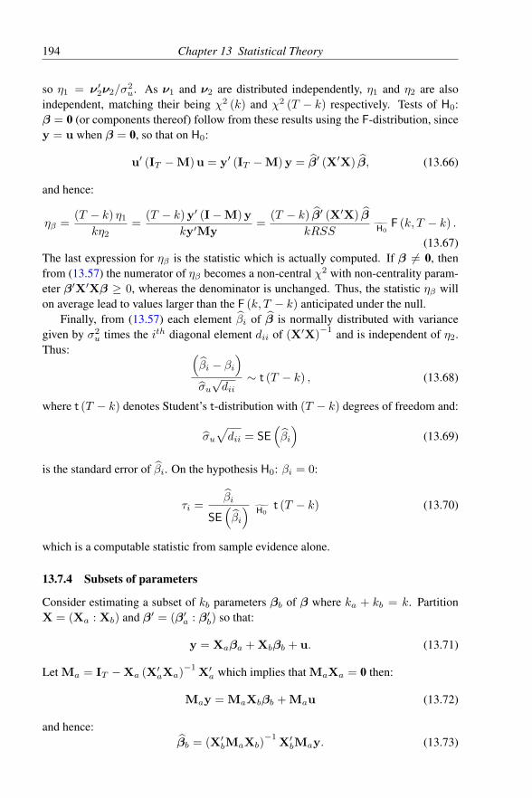
194 Chapter 13 Statistical Theory
so η1 = ν′2ν2/σ2u. As ν1 and ν2 are distributed independently, η1 and η2 are also
independent, matching their being χ2 (k) and χ2 (T − k) respectively. Tests of H0:β = 0 (or components thereof) follow from these results using the F-distribution, sincey = u when β = 0, so that on H0:
u′ (IT −M) u = y′ (IT −M) y = β′ (X′X) β, (13.66)
and hence:
ηβ =(T − k) η1
kη2=
(T − k) y′ (I−M) y
ky′My=
(T − k) β′ (X′X) β
kRSS H0F (k, T − k) .
(13.67)The last expression for ηβ is the statistic which is actually computed. If β 6= 0, thenfrom (13.57) the numerator of ηβ becomes a non-central χ2 with non-centrality param-eter β′X′Xβ ≥ 0, whereas the denominator is unchanged. Thus, the statistic ηβ willon average lead to values larger than the F (k, T − k) anticipated under the null.
Finally, from (13.57) each element βi of β is normally distributed with variancegiven by σ2
u times the ith diagonal element dii of (X′X)−1 and is independent of η2.
Thus: (βi − βi
)σu√dii
∼ t (T − k) , (13.68)
where t (T − k) denotes Student’s t-distribution with (T − k) degrees of freedom and:
σu√dii = SE
(βi
)(13.69)
is the standard error of βi. On the hypothesis H0: βi = 0:
τi =βi
SE(βi
)H0
t (T − k) (13.70)
which is a computable statistic from sample evidence alone.
13.7.4 Subsets of parameters
Consider estimating a subset of kb parameters βb of β where ka + kb = k. PartitionX = (Xa : Xb) and β′ = (β′a : β′b) so that:
y = Xaβa + Xbβb + u. (13.71)
Let Ma = IT −Xa (X′aXa)−1
X′a which implies that MaXa = 0 then:
May = MaXbβb + Mau (13.72)
and hence:βb = (X′bMaXb)
−1X′bMay. (13.73)

13.7 Multiple regression 195
Consequently, βb can be calculated by first regressing Xb on Xa and saving the resid-uals (MaXb), then regressing y on those residuals. Notice that the regressors need‘corrected’, but the regressand does not. Thus, procedures for ‘detrending’ (for exam-ple), can be justified as equivalent to adding a trend to the model (see Frisch and Waugh,1933, who first proved this famous result). From (13.72) and (13.73):
βb = βb + (X′bMaXb)−1
X′bMau (13.74)
so thatV[βb
]= σ2
u (X′bMaXb)−1. (13.75)
Thus:βb ∼ Nkb
[βb, σ
2u (X′bMaXb)
−1]. (13.76)
Hypothesis tests about βb follow analogously to the previous section. In particular,from §13.7.3 and (13.76):
ηb =
(βb − βb
)′(X′bMaXb)
(βb − βb
)kbσ2
u
∼ F (kb, T − k) . (13.77)
When kb = 1, this matches (13.70) under H0: βb = 0, and when kb = k, (13.77)reproduces (13.67) under H0: β = 0. A useful case of (13.77) is kb = (k − 1) andXa = ι (a T × 1 vector of ones), so all coefficients other than the intercept are tested.
If, instead of estimating (13.71), Xa is omitted from the model in the incorrectbelief that βa = 0, the equation to be estimated becomes:
y = Xbβb + e (13.78)
The resulting estimator of βb, denoted by βb = (X′bXb)−1
X′by, confounds the effectsof Xa and Xb:
βb = (X′bXb)−1
X′b (Xaβa + Xbβb + u)
= Bbaβa + βb + (X′bXb)−1
X′bu(13.79)
where Bba = (X′bXb)−1
X′bXa. Thus:
E[βb
]= Bbaβa + βb, (13.80)
which equals βb if and only if Bbaβa = 0. Moreover, let Mb have the same form asMa but using Xb then:
V[βb
]= σ2
u (X′bXb)−1 where σ2
u =y′Mby
(T − kb)=
u′u
(T − kb)(13.81)
when u = y −Xbβb and:
E[σ2u
]= σ2
u +β′aX
′aMbXaβa
(T − kb)≥ σ2
u. (13.82)

196 Chapter 13 Statistical Theory
Conventionally, βb is interpreted as a biased estimator of βb with bias given by Bbaβa.The estimated variance matrix in (13.81) may exceed, or be less than, that given bythe relevant sub-matrix of (13.56), in the sense that the difference could be positive ornegative semi-definite.
The sign of an estimated coefficient from (13.78) can be the same as, or the oppositeto, that expected from prior theoretical reasoning, and the latter is sometimes called a‘wrong sign’. We interpret the outcome in (13.80) as delivering a different coefficientγb = Bbaβa + βb than βb, consonant with the following argument. First:
Xa ≡MbXa + (IT −Mb) Xa = MbXa + XbBba. (13.83)
Consequently, from (13.71):
y = (MbXa + XbBba)βa + Xbβb + u
= Xbγb + (u + MbXaβa)
= Xbγb + v
(13.84)
where E [v] = MbXaβa 6= 0, but since MbXb = 0:
E [X′bv] = E [X′bu] + X′bMbXaβa = 0. (13.85)
Thus, the model is implicitly reparametrized by omitting Xa, and OLS is an unbiasedestimator of γb despite E [v] 6= 0. Under more general assumptions, a related large-sample result holds.
13.7.5 Partitioned inversion
The results on estimating subsets of parameters can be obtained by partitioned inversionof (X′X). Consider the matrix (X′X)
−1. Let H = (X′bMaXb) and G = (X′aMbXa),then:(
X′aXa X′aXb
X′bXa X′bXb
)−1
=
((X′aMbXa)
−1 − (X′aMbXa)−1
B′ba−Bab (X′bMaXb)
−1(X′bMaXb)
−1
)(13.86)
where Bab = (X′aXa)−1
X′aXb. Further, X′y can be partitioned conformably as:(X′ay
X′by
)(13.87)
and multiplication of (13.87) by (13.86) delivers (13.73) together with correspondingexpressions for estimating βa; the coefficient variance matrix follows from (13.86).
Alternatively, when (X′X)−1 is given by:(
(X′aMbXa)−1 − (X′aMbXa)
−1B′ba
−Bba (X′aMbXa)−1
(X′bXb)−1
+ Bba (X′aMbXa)−1
B′ba
)(13.88)
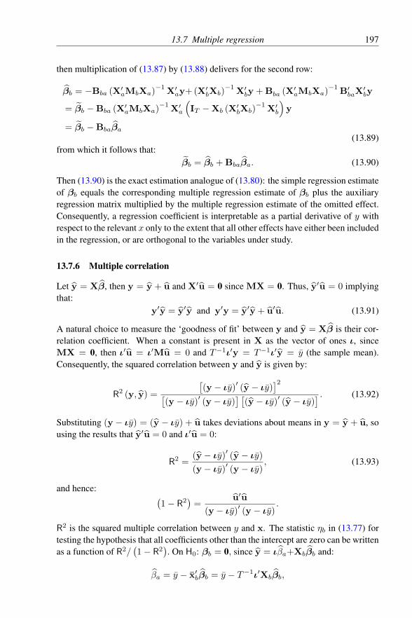
13.7 Multiple regression 197
then multiplication of (13.87) by (13.88) delivers for the second row:
βb = −Bba (X′aMbXa)−1
X′ay+ (X′bXb)−1
X′by + Bba (X′aMbXa)−1
B′baX′by
= βb −Bba (X′aMbXa)−1
X′a
(IT −Xb (X′bXb)
−1X′b
)y
= βb −Bbaβa(13.89)
from which it follows that:βb = βb + Bbaβa. (13.90)
Then (13.90) is the exact estimation analogue of (13.80): the simple regression estimateof βb equals the corresponding multiple regression estimate of βb plus the auxiliaryregression matrix multiplied by the multiple regression estimate of the omitted effect.Consequently, a regression coefficient is interpretable as a partial derivative of y withrespect to the relevant x only to the extent that all other effects have either been includedin the regression, or are orthogonal to the variables under study.
13.7.6 Multiple correlation
Let y = Xβ, then y = y + u and X′u = 0 since MX = 0. Thus, y′u = 0 implyingthat:
y′y = y′y and y′y = y′y + u′u. (13.91)
A natural choice to measure the ‘goodness of fit’ between y and y = Xβ is their cor-relation coefficient. When a constant is present in X as the vector of ones ι, sinceMX = 0, then ι′u = ι′Mu = 0 and T−1ι′y = T−1ι′y = y (the sample mean).Consequently, the squared correlation between y and y is given by:
R2 (y, y) =
[(y − ιy)
′(y − ιy)
]2[(y − ιy)
′(y − ιy)
] [(y − ιy)
′(y − ιy)
] . (13.92)
Substituting (y − ιy) = (y − ιy) + u takes deviations about means in y = y + u, sousing the results that y′u = 0 and ι′u = 0:
R2 =(y − ιy)
′(y − ιy)
(y − ιy)′(y − ιy)
, (13.93)
and hence: (1− R2
)=
u′u
(y − ιy)′(y − ιy)
.
R2 is the squared multiple correlation between y and x. The statistic ηb in (13.77) fortesting the hypothesis that all coefficients other than the intercept are zero can be writtenas a function of R2/
(1− R2
). On H0: βb = 0, since y = ιβa+Xbβb and:
βa = y − x′bβb = y − T−1ι′Xbβb,

198 Chapter 13 Statistical Theory
then:y = ιy − T−1ιι′Xbβb+Xbβb = ιy + MaXbβb,
as Ma =(IT − ι (ι′ι)
−1ι′)
=(IT − T−1ιι′
), so that:
ηb =(T − k) β
′
bX′bMaXbβb
(k − 1) u′u=
(T − k) (y − ιy)′(y − ιy)
(k − 1) u′u=
(T − k) R2
(k − 1) (1− R2).
(13.94)As R2 → 1, highly ‘significant’ results are bound to occur independently of their sub-stance.
13.7.7 Partial correlation
The notion of a partial correlation, or a partial regression coefficient, is fundamental tointerpreting econometric evidence. For empirical modelling, equations like (13.48) areusually formulated with the implicit assumption that:
∂yt∂xit
= βi for i = 1, . . . , k. (13.95)
OLS estimates βi are then interpreted as if they had the same properties. When i = b,βb is a scalar so that Xb is a vector xb, and the marginal distribution of βb is given in(13.76). Then the partial correlation rby·a between y and xb having removed the linearinfluence of Xa (assumed to contain ι) is the correlation between May and Maxb:
rby·a =y′Maxb√
(y′May) (x′bMaxb)=βb√
(x′bMaxb)√(y′May)
. (13.96)
Note that May and Maxb have zero means and that:
r2by·a =
βb (x′bMaxb) βby′May
. (13.97)
The numerator of (1− r2by·a) is y′May − βb (x′bMaxb) βb = y′M∗y where:
M∗ = Ma −Maxb (x′bMaxb)−1
x′bMa
= Ma
[IT −Maxb (x′bMaxb)
−1x′bMa
]Ma
(13.98)
so M∗ = M. This last equality follows from applying (13.86) since [·] annihilatesMaxb. As a check, by suitable rearrangement of the order of regressors, M∗X =
M∗ (Xa : xb) = 0 = MX. From the earlier formula for τi when i = b:
τ2b =
(T − k) r2by·a(
1− r2by·a
) , (13.99)
In the special case that k = 2 and xa = ι, (13.94) coincides with (13.99).

13.7 Multiple regression 199
When Xa includes ι and kb > 1, (13.98) holds in the form:
M = Ma −MaXb (X′bMaXb)−1
X′bMa,
so that:
y′My = y′May − y′MaXb (X′bMaXb)−1
X′bMay = y′May − β′
bX′bMaXbβb.
(13.100)Substituting (13.100) in (13.77):
ηb =(T − k) (y′May − y′My)
kbu′u=
(T − k) (u′u− u′u)
kbu′u=
(T − k)
kb
(dσ2u
σ2u
− 1
)(13.101)
where d = (T − ka) / (T − k). Thus, when σ2u = σ2
u, ηb = 1 and when σ2u > σ2
u,ηb < 1. Deleting kb regressors when the F-test for the significance of their coefficientsis less than unity will lower the estimated residual standard error. For kb = 1, deletinga single variable with τ2
b < 1 will lower the estimated residual standard error.
13.7.8 Maximum likelihood estimation
As noted, OLS is also the MLE here. When u ∼ NT [0, σ2uI], the conditional log-
likelihood function is:
`(β,σ2
u | X; y)
= −T2
log (2π)− T
2log(σ2u
)− (y −Xβ)
′(y −Xβ)
2σ2u
(13.102)
so the MLE minimizes the last term, which yields OLS. From above:
`(β,σ2
u | X; y)
= −T2
log (2π)− T
2log(σ2u
)−
(β − β
)′X′X
(β − β
)2σ2
u
− u′u
2σ2u
(13.103)From (13.103), (β, σ2
u) are jointly sufficient for(β,σ2
u
), and by independence, the joint
distribution of β and σ2u factorizes into the products of their marginals.
13.7.9 Recursive estimation
To understand the basis of recursive estimation, denote the specified equation by:
yt = β′xt + ut (13.104)
where β is asserted to be constant, E [xtut] = 0∀t, E(u2t
)= σ2
u, and E (utus) = 0
if t 6= s. Let the complete sample period be (1, . . . , T ), and consider the least-squaresoutcome on a subsample up to t− 1 (for t > k when there are k regressors in xt−1):
βt−1 =(X′t−1Xt−1
)−1X′t−1yt−1, (13.105)
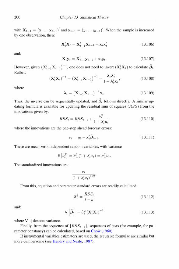
200 Chapter 13 Statistical Theory
with Xt−1 = (x1 . . .xt−1)′ and yt−1 = (y1 . . . yt−1)
′. When the sample is increasedby one observation, then:
X′tXt = X′t−1Xt−1 + xtx′t (13.106)
and:X′tyt = X′t−1yt−1 + xtyt. (13.107)
However, given(X′t−1Xt−1
)−1, one does not need to invert (X′tXt) to calculate βt.
Rather:
(X′tXt)−1
=(X′t−1Xt−1
)−1 − λtλ′t
1 + λ′txt, (13.108)
whereλt =
(X′t−1Xt−1
)−1xt. (13.109)
Thus, the inverse can be sequentially updated, and βt follows directly. A similar up-dating formula is available for updating the residual sum of squares (RSS) from theinnovations given by:
RSSt = RSSt−1 +ν2t
1 + λ′txt(13.110)
where the innovations are the one-step ahead forecast errors:
νt = yt − x′tβt−1. (13.111)
These are mean zero, independent random variables, with variance
E[ν2t
]= σ2
u (1 + λ′txt) = σ2uωt.
The standardized innovations are:
νt
(1 + λ′txt)1/2
.
From this, equation and parameter standard errors are readily calculated:
σ2t =
RSStt− k
(13.112)
and:V[βt
]= σ2
t (X′tXt)−1 (13.113)
where V [·] denotes variance.Finally, from the sequence of RSSt−1, sequences of tests (for example, for pa-
rameter constancy) can be calculated, based on Chow (1960).If instrumental variables estimators are used, the recursive formulae are similar but
more cumbersome (see Hendry and Neale, 1987).
Chapter 14
Advanced Econometrics
14.1 IntroductionThis chapter offers an overall description of the class of dynamic models handled byPcGive, the most frequently used concepts and modelling strategies, and the estima-tion and evaluation procedures available. The class of single-equation dynamic linearmodels analyzed by PcGive, including a model typology and distinctions between in-terpretations of linear models, were described in Chapter 12. Here we discuss dynamicsystems in §14.2. The crucial concept of weak exogeneity is described in §14.3.2 as thebasis for valid inference in single-equation conditional models which are neverthelesspart of a dynamic economic system. That section also introduces several factorizationsof data density functions, and relates these to such concepts as white noise and innova-tions. Following a brief overview of estimation techniques in §14.4 the discussion thenturns to model evaluation in §14.5, the types of test used in §14.6, and an informationtaxonomy for model evaluation and design in §14.7. Finally, section 14.8 considersmodelling strategies with an emphasis on automatic model selection.
14.2 Dynamic systemsThe class of models basic to PcGive is that of linear dynamic single equations. Chap-ter 12 discussed the formulation and properties of such equations, their forms (in thetypology), and their different interpretations. In economics, however, equations cannotbe viewed in isolation: they are inherently part of a system. Here we note the structureof such systems, and lay the ground for determining when a single-equation analysis islikely to be valid despite the system context. Volume II (Doornik and Hendry, 2013c)analyzes linear dynamic systems qua systems, but PcGive provides single-equationmethods that are applicable when one equation is the focus of interest from a system thatotherwise is rather loosely specified. Dynamic systems are more extensively describedin Volume II. For completeness, we give a brief overview here.
201
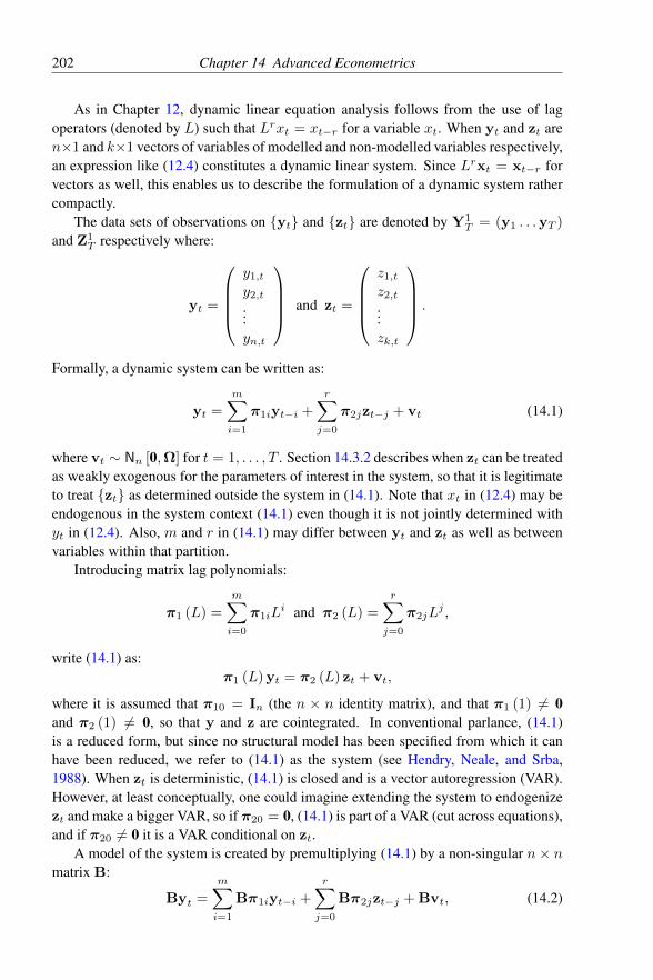
202 Chapter 14 Advanced Econometrics
As in Chapter 12, dynamic linear equation analysis follows from the use of lagoperators (denoted by L) such that Lrxt = xt−r for a variable xt. When yt and zt aren×1 and k×1 vectors of variables of modelled and non-modelled variables respectively,an expression like (12.4) constitutes a dynamic linear system. Since Lrxt = xt−r forvectors as well, this enables us to describe the formulation of a dynamic system rathercompactly.
The data sets of observations on yt and zt are denoted by Y1T = (y1 . . .yT )
and Z1T respectively where:
yt =
y1,t
y2,t
...yn,t
and zt =
z1,t
z2,t
...zk,t
.
Formally, a dynamic system can be written as:
yt =
m∑i=1
π1iyt−i +
r∑j=0
π2jzt−j + vt (14.1)
where vt ∼ Nn [0,Ω] for t = 1, . . . , T . Section 14.3.2 describes when zt can be treatedas weakly exogenous for the parameters of interest in the system, so that it is legitimateto treat zt as determined outside the system in (14.1). Note that xt in (12.4) may beendogenous in the system context (14.1) even though it is not jointly determined withyt in (12.4). Also, m and r in (14.1) may differ between yt and zt as well as betweenvariables within that partition.
Introducing matrix lag polynomials:
π1 (L) =
m∑i=0
π1iLi and π2 (L) =
r∑j=0
π2jLj ,
write (14.1) as:π1 (L) yt = π2 (L) zt + vt,
where it is assumed that π10 = In (the n × n identity matrix), and that π1 (1) 6= 0and π2 (1) 6= 0, so that y and z are cointegrated. In conventional parlance, (14.1)is a reduced form, but since no structural model has been specified from which it canhave been reduced, we refer to (14.1) as the system (see Hendry, Neale, and Srba,1988). When zt is deterministic, (14.1) is closed and is a vector autoregression (VAR).However, at least conceptually, one could imagine extending the system to endogenizezt and make a bigger VAR, so if π20 = 0, (14.1) is part of a VAR (cut across equations),and if π20 6= 0 it is a VAR conditional on zt.
A model of the system is created by premultiplying (14.1) by a non-singular n× nmatrix B:
Byt =
m∑i=1
Bπ1iyt−i +
r∑j=0
Bπ2jzt−j + Bvt, (14.2)

14.2 Dynamic systems 203
or switching notation:
B (L) yt = C (L) zt + ut with ut ∼ INn [0,Σ] . (14.3)
The system is said to be complete if B is non-singular. Let A be the matrix of all thecoefficients:
A = (B0 : B1 : · · · : Bm : −C0 : · · · : −Cr)
and xt the column vector of all the variables (yt . . .yt−m : zt . . . zt−r) then (14.3) canbe written neatly as:
Axt = ut ∼ INn [0,Σ] .
The matrix A must be restricted if the Bi,Ci are to be unique: otherwise, afurther non-singular multiplication of (14.2) would produce a different model, yet onewhich looked exactly like (14.3), thereby destroying uniqueness. The rank and orderconditions for identification apply: both are fully discussed in Volume II. The mainissue of relevance to PcGive is that in any equation containing p right-hand side en-dogenous variables, the system of which it is part must contain at least p non-modelledvariables not included in that equation: this is the order condition. When the sample ofT observations on these p endogenous variables is just denoted by Y and the sampleon the excluded but available non-modelled variables is Z, then:
rank (Y′Z) = p,
is both necessary and sufficient for identification: this is the rank condition (see White,1984).
All of the model types of §12.4 could occur within (14.3), and if A is over-identified,the imposed restrictions are testable. When developing a model of a system, it is sensi-ble to commence from the unrestricted representation (14.1), test its validity, and thenreduce the system to the model. All of the attributes needed for the model to match theevidence are called congruency (see §14.7) and these can be tested, but care is requiredin modelling integrated data. As a first step, cointegration tests can be conducted toestablish the dimension of the cointegrating space, and the relevant set of cointegrationrestrictions and differences can be imposed to reduce the data to I(0). This order will fa-cilitate later testing, since conventional limiting distributions can be used: see Phillips(1991) and Hendry and Mizon (1993) for discussions of modelling cointegrated pro-cesses, Johansen (1988) and Johansen and Juselius (1990) for analyses of the maximumlikelihood estimator, and Hendry, Neale, and Srba (1988) for an approach to structuralsystem modelling in I(0) processes. Such a methodology implements the general-to-specific notion in the system context, and contrasts with the alternative of specifying astructural model at the outset and testing its restrictions against the (derived) reducedform. Since the latter may be invalid, it provides an unreliable benchmark for any tests.Techniques for estimating models, as well as general derivations of standard errors etc.,are considered in §14.4 below; further detail on systems and models thereof is providedin Volume II, which includes the implementation of a complete modelling exercise ona dynamic cointegrated system.

204 Chapter 14 Advanced Econometrics
Prior to proceeding, we note that since (14.1) is a model of itself, and there arelikely to be valid parsimonious representations of the system (14.1), the critique in Sims(1980) lacks force. Specifying a model in structural form corresponds to imposing non-linear restrictions across functions of the πs in (14.1), and there are no a priori groundsfor claiming that all possible restrictions are invalid. For example, if the response ofy1,t to y2,t is very rapid compared to that of y2,t to y1,t in a second equation, a struc-tural model of their joint representation can impose valid restrictions on the VAR. Theapplication of encompassing discussed in §14.7 will clarify this issue further. At theheart of the issue of conditional estimation is the role of weak exogeneity in modellingsingle equations, so we now discuss that issue (see Engle, Hendry, and Richard, 1983).
14.3 Data density factorizationsTo undertake valid inference using a single-equation approach, some conditions mustbe fulfilled such that the system dependence of conditioning variables can be neglectedwithout losing relevant information. These conditions are encapsulated in the conceptof weak exogeneity. First, we introduce joint data density functions, and extend thenotion of factorization introduced in Chapter 13.
14.3.1 Innovations and white noise
The data set of observations on yt and zt in (14.1) is denoted by X1T = (x1 . . .xT )
where x′t = (y′t : z′t). Thus:
X1T =
(y1 y2 · · · yTz1 z2 · · · zT
).
Denote the process generating X1T by DX
(X1T |θ1
T ,X0
)where X0 are the initial con-
ditions and θ1T ∈ Θ are the ‘parameters’ of the process, which may depend on the
historical time (hence the indexing by 1, . . . , T ). Since X1T = (x1 . . .xT ), the whole
sample data density DX (·) can be sequentially factorized as the product of terms likeDx
(xt|X1
t−1,θt,X0
)which is each time period’s density. This exploits the fact that if
P (a) denotes the probability of an event a, then P (ab) = P (a|b) P (b), and this canbe repeated starting at t, then t − 1, . . . , 1. Assume θt = θ ∀t (constancy is the topicof §14.7.3), and let Xt−1 =
(X1t−1,X0
)so that DX (·) at every t is Dx (xt|θ,Xt−1).
Then:
DX
(X1T | θ,X0
)=
T∏t=1
Dx (xt | θ,Xt−1) . (14.4)
Let:νt = xt − E [xt | Xt−1] ,
then by construction, νt is a mean innovation process since:
E [νt | Xt−1] = E [(xt − E [xt | Xt−1]) | Xt−1] = 0. (14.5)

14.3 Data density factorizations 205
Moreover, since lagged νs, denoted by Vt−1, can be derived from Xt−1 (by laggingtheir definition), they are also white noise:
E [νt | Vt−1] = 0. (14.6)
Thus, the DGP can be expressed without loss in an innovation-error representation.A well-known example is provided by the stationary first-order autoregressive pro-
cess:yt = µyt−1 + et,
when et is jointly normal and E [etes] = 0 ∀t 6= s. Then, DY
(y1 . . . yT |µ, σ2
e , y0
)is the multivariate normal density NT
[0, σ2
eΩ]
where Ω is a T × T symmetric matrixwith (i, j)
th element:µ|i−j|
(1− µ2).
The factorization of the joint density of (y1 . . . yT ) is:
DY
(y1 . . . yT | µ, σ2
e , y0
)=
T∏t=1
Dy
(yt | Yt−1;µ, σ2
e
)which yields a product of individual density terms like N
[µyt−1, σ
2e
]. Since νt =
yt − E (yt|Yt−1), then:
νt = yt − E [yt | yt−1] = yt − µyt−1 = et
is indeed the (mean) innovation (see e.g., Judge, Griffiths, Hill, Lutkepohl, and Lee,1985, Chapter 8).
14.3.2 Weak exogeneity
We can now formalize weak exogeneity. Its importance is that all current-dated re-gressors treated as conditioning variables must be weakly exogenous to sustain validand efficient inferences (see Engle, Hendry, and Richard, 1983). To relate the analysismore closely to that in Chapter 12, we only consider a bivariate system, where the twovariables are (yt : zt): the analysis generalizes by interpreting these as vectors.
First, note that the joint density Dx (xt|θ,Xt−1) is unaffected by 1-1 transforma-tions of its parameters θ to φ (say) where:
φ = f (θ) and φ ∈ Φ,
so that:Dx (xt | θ,Xt−1) = Dx (xt | φ,Xt−1) .
Secondly, we can partition into φ = (φ1 : φ2) to match the partition of xt into(yt : zt). Then, using the factorization in (14.4), if yt is to be conditioned on zt, we canfactorize Dx (·) into a conditional and a marginal distribution:
Dx (xt | θ,Xt−1) = Dy|z (yt | zt,Xt−1,φ1) Dz (zt | Xt−1,φ2) . (14.7)

206 Chapter 14 Advanced Econometrics
This does not impose any restrictions, and hence loses no information.Thirdly, some parameters, denoted µ, will be the focus of the econometric mod-
elling exercise, and these are called parameters of interest. To avoid information lossfrom only modelling the conditional relation in (14.7), it must be possible to learn aboutµ from the factor:
Dy|z (yt | zt,Xt−1,φ1) (14.8)
alone. Moreover, the resulting knowledge about µ must be equivalent to that whichcould have been gleaned from analyzing the joint density Dx (·). Two conditions ensurethat equivalence. First:1. all the parameters of interest µ can be obtained from φ1 alone; and2. φ1 and φ2 must be variation free (that is, impose no restrictions on each other):
(φ1 : φ2) ∈ Φ1 ×Φ2 where φ1 ∈ Φ1 and φ2 ∈ Φ2.
If so, zt is said to be weakly exogenous for µ, and only the conditional modelDy|z (yt|zt,Xt−1,φ1) needs to be estimated to determine µ, since the marginal modelDz (zt|Xt−1,φ2) contains no information about µ. For more extensive and expositorydiscussions, see Ericsson (1992) and Hendry (1995a).
14.4 Model estimation
Like many of the other aspects considered here, appropriate estimation is a necessary,rather than a sufficient, condition for developing useful models. Given a particularmodel form and a distributional assumption about the data, the log-likelihood functioncan be formulated, and is denoted ` (θ) where θ is the vector of unknown parametersof interest. Maximum likelihood (MLE) and least squares estimators are described inChapter 13. In some cases, the set of first-order conditions defining the MLE maybe non-linear and require iterative solution methods: this holds for any non-linear re-gression model. In large samples, for correctly specified problems, MLEs have manyexcellent statistical properties. Moreover, for models linear in both variables and pa-rameters, almost all other estimation methods can be obtained as approximate solutionsof the score equation based on choosing different initial values and selecting differentnumbers of iterative steps in alternative numerical methods. For example, simultaneousequations estimation is encapsulated in a simple formula called the estimator generatingequation (EGE: see Hendry, 1976, and Hendry, Neale, and Srba, 1988). Here we notethat OLS and IVE are special cases of the EGE when an individual equation is beingstudied (even if that equation is implicitly part of a system).
The standard errors of θ are usually calculated from the inverse of the informa-tion matrix or the negative inverse of the Hessian, although such a formula assumes acorrectly-specified error (that is, a homoscedastic innovation). In PcGive, autocorrela-tion and heteroscedastic-consistent standard errors can be computed for OLS, but anydifferences from the conventional SEs reveals non-congruence.
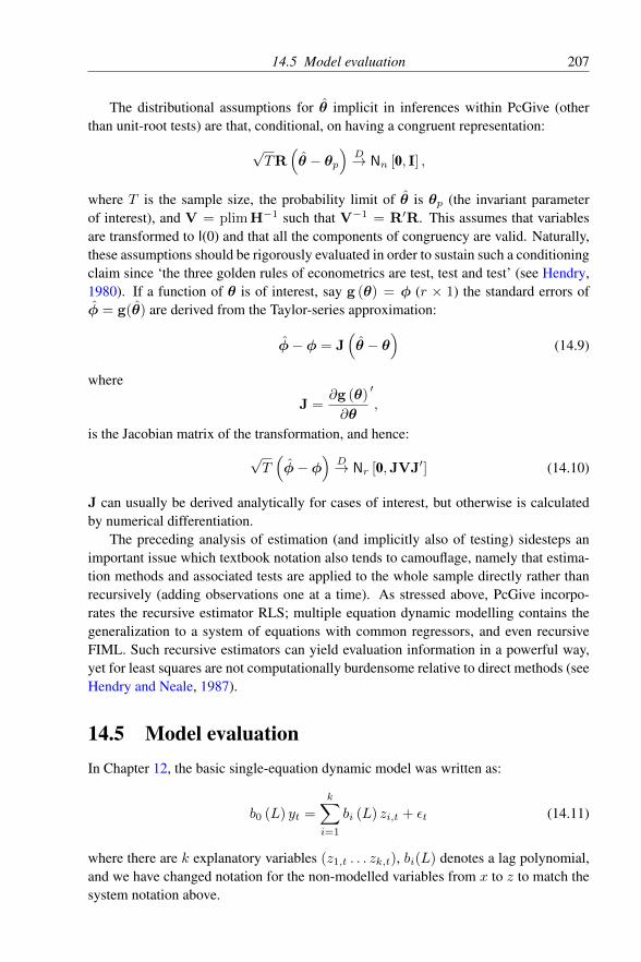
14.5 Model evaluation 207
The distributional assumptions for θ implicit in inferences within PcGive (otherthan unit-root tests) are that, conditional, on having a congruent representation:
√TR
(θ − θp
)D→ Nn [0, I] ,
where T is the sample size, the probability limit of θ is θp (the invariant parameterof interest), and V = plim H−1 such that V−1 = R′R. This assumes that variablesare transformed to I(0) and that all the components of congruency are valid. Naturally,these assumptions should be rigorously evaluated in order to sustain such a conditioningclaim since ‘the three golden rules of econometrics are test, test and test’ (see Hendry,1980). If a function of θ is of interest, say g (θ) = φ (r × 1) the standard errors ofφ = g(θ) are derived from the Taylor-series approximation:
φ− φ = J(θ − θ
)(14.9)
where
J =∂g (θ)
∂θ
′,
is the Jacobian matrix of the transformation, and hence:√T(φ− φ
)D→ Nr [0,JVJ′] (14.10)
J can usually be derived analytically for cases of interest, but otherwise is calculatedby numerical differentiation.
The preceding analysis of estimation (and implicitly also of testing) sidesteps animportant issue which textbook notation also tends to camouflage, namely that estima-tion methods and associated tests are applied to the whole sample directly rather thanrecursively (adding observations one at a time). As stressed above, PcGive incorpo-rates the recursive estimator RLS; multiple equation dynamic modelling contains thegeneralization to a system of equations with common regressors, and even recursiveFIML. Such recursive estimators can yield evaluation information in a powerful way,yet for least squares are not computationally burdensome relative to direct methods (seeHendry and Neale, 1987).
14.5 Model evaluationIn Chapter 12, the basic single-equation dynamic model was written as:
b0 (L) yt =
k∑i=1
bi (L) zi,t + εt (14.11)
where there are k explanatory variables (z1,t . . . zk,t), bi(L) denotes a lag polynomial,and we have changed notation for the non-modelled variables from x to z to match thesystem notation above.

208 Chapter 14 Advanced Econometrics
It is relatively easy to specify and analyze models such as those in (14.11), or anygeneralizations thereof, when they are regarded as mathematical formulations. Unfor-tunately, it is far more difficult to develop useful empirical relationships correspondingto these for a given time series on a set of variables. In particular, the orders of the laglengths of every polynomial b0 (L), b1 (L) etc. must be established, as must the rele-vance of any given variable, the constancy of the entities called parameters, the validityof conditioning, the required functional form, and the properties of the unmodelledterm. Indeed, this description begs the very issue of what defines the usefulness of aneconometric relationship.
At a general level, the utility of anything depends on the purposes for which it isbeing developed. Hence if a completely specified loss function existed for judging aparticular modelling exercise, it would seem natural to develop a model to optimizethat criterion. Two problems arise, however, neither of which can be sidestepped. First,it is rare in econometrics to be able to fully specify the loss function. Models are wantedfor prediction, for scenario or policy analyses, for testing economic hypotheses, and forunderstanding how the economy functions. Empirically, there often exist conflicts incriteria in selecting models to achieve such multiple objectives. For example, a modelwhich predicts well historically may yield no insight into how a market will behaveunder some change in regulations, the implementation of which will cause that modelto mispredict. Secondly, even assuming that a fully-specified loss function did exist andthat the optimal model could be selected, there remains the difficulty of establishinghow ‘good’ that best model is. For example, the best model that could be found maystill suffer from non-constant parameters and hence yield a low level of utility; worsestill, by not knowing this weakness, serious losses may accrue in the future. Thus,whatever the basis on which a model has been formulated or developed, there remainsan issue of assessment or evaluation.
PcGive operates easily and efficiently to implement this aspect. Since we do notknow how the economy works, we do not know the best way of studying it. Conse-quently, any model might correspond to reality, however unlikely its mode of creation;or unfortunately, it might transpire to be invalid, however clever and thorough its devel-opment. Nevertheless, taking a model as stated by its proprietor, a vast range of statesof the world will be excluded by that model, and thus it is open to evaluation against theavailable information (see Hendry, 1987, for a more extensive analysis). For example,because its residual process is white noise, a particular model may claim to explain agiven data set adequately; yet the residuals may not be an innovation process, so testingthat latter hypothesis might reveal an important model weakness (as in the COMFACprocedure discussed in §12.4). This is the destructive testing aspect of PcGive, andaccounts for its wide range of pre-programmed statistics for model evaluation.
Testing focuses on the empirical validity of assertions about a given model. Testsare statistics with a known distribution under a null hypothesis and some power againsta specific alternative. The tests below are designed to have (central) t, F or χ2 distri-butions under the null, and corresponding non-central distributions against some alter-native. Usually, they are invariant to the direction of the departure from the null for
14.6 Test types 209
a given class of alternatives, and only depend on the distance (that is, the overall ex-tent of the departure: this holds for t2, F and χ2 statistics). However, most tests alsohave some power to detect other alternatives, so rejecting the null does not entail ac-cepting the alternative, and in many instances, accepting the alternative would be a nonsequitur. Rejection reveals model invalidity, albeit with some chance of a type-I errorof incorrectly rejecting a valid null.
First, however, we need to delineate the relevant class of null hypotheses, and thenderive associated test statistics for reasonable alternatives. The former task is consid-ered in §14.7 in terms of a taxonomy of available information, and the latter in §14.6where the main test principles are briefly described.
14.6 Test types
Various test principles are commonly used in econometrics and the three main onesare Wald (W), Lagrange-multiplier (LM) and Likelihood-ratio (LR) tests (see Breuschand Pagan, 1980, and Engle, 1984). For example, the Chow (1960) test for parame-ter constancy is derivable from all three principles, whereas the test of over-identifyingrestrictions is LR, the portmanteau tests for autocorrelation in OLS are based on LM,and the COMFAC tests are Wald tests. In each instance, the choice of test type tendsto reflect computational ease. Under the relevant null hypothesis and for local alter-natives, the three test types are asymptotically equivalent; however, if equations aremis-specified in other ways than that under test, or the sample size is small, differentinferences can result.
Although LM tests conventionally come in the form TR2 (being distributed as χ2),research indicates that F-forms have more appropriate significance levels and that χ2
versions reject acceptable models too often (see Kiviet, 1987). (Incidentally, Kiviet’sresults also show that the Chow test and LM tests for autocorrelated residuals are ap-proximately independently distributed.) Thus, PcGive tends to report F-forms whenpossible. Pagan (1984) exposits testing in terms of residual diagnostic procedures. Fur-ther details on econometric testing can be found in Harvey (1981), Harvey (1990),Spanos (1986), Godfrey (1988), Hendry (1995a) or in relevant chapters of Grilichesand Intriligator (1984).
While a basic feature of PcGive is that most of the test statistics are calculated by asimple choice from a menu, others are inbuilt. For example, parameter constancy testsbased on Hansen (1992) can be automatically undertaken with OLS estimation; alter-natively, if the user initially specifies some post-sample observations, forecast-basedtests are computed. Similar considerations apply to tests for the validity of any givenchoice of instrumental variables (automatic), and to the significance of lagged variables(computed by selecting Dynamic analysis). Note that the options in the Options dialog
can be set to ensure automatic computation of the test summary, inter alia.

210 Chapter 14 Advanced Econometrics
14.7 An information taxonomy
A further division of the data set X1t = (x1 . . .xt) into:
X1T =
(X1t−1 : xt : Xt+1
T
)yields the trichotomy of the (past : present : future) relative to t. In addition, we allowfor theory information, measurement information, and the information in rival models(see Hendry and Richard; Hendry and Richard, 1982, 1983, and Gilbert, 1986, for ex-positions). Statistical tests can be constructed to evaluate a model against each elementof this six-fold taxonomy. Such tests require formulating both the appropriate null hy-pothesis for the relevant information set, and devising a reasonable class of alternativesagainst which the test should have power. The taxonomy clarifies the relevant null hy-potheses, and generally points up interesting alternatives against which to test modelvalidity.
The six major aspects of model evaluation are discussed next, followed by a briefanalysis of their relation to the theory of reduction.
14.7.1 The relative past
The residuals should be white noise and hence unpredictable from their own past asin (14.6). This entails that they should not be significantly autocorrelated. If they areautocorrelated, a better-fitting model can be developed by removing the autocorrela-tion, although this is not a recommended practice, since it may impose invalid commonfactors. PcGive provides valid tests and diagnostic information for residual autocorre-lation, including Lagrange-multiplier tests for a wide range of orders of autoregressiveerrors, as well as residual correlograms and autoregressions.
Further, the errors should not be explainable from the information set being used.Alternatively expressed, the errors should be an innovation process which is unpre-dictable from lagged functions of the available data as in (14.5). Being white noise isa necessary, but not sufficient, condition for being an innovation, as shown above. Agood example arises when removing autocorrelation by fitting, say, autoregressive er-ror processes, since that automatically ensures the white noise, but may impose invalidcommon-factor restrictions and hence does not entail an innovation error (see Sargan;Sargan, 1964, 1980a). This problem can be avoided by beginning with a general spec-ification like (14.11) and testing for valid common factors prior to imposing them. InPcGive, the COMFAC tests to check such restrictions are based on Sargan’s algorithms.
Neither white-noise errors nor innovations need be homoscedastic, so that the stan-dard errors of OLS estimators in PcGive can allow for residual heteroscedasticity (theHCSEs in Chapter 12: see White, 1980, and MacKinnon and White, 1985). Tests ofboth autoregressive conditional heteroscedasticity (ARCH: see Engle, 1982) and uncon-ditional heteroscedasticity are also provided. Similarly, tests for normality are includedto check on the distributional assumptions underlying finite-sample inference.

14.7 An information taxonomy 211
To summarize these aspects relating to the (relative) past of the process, namelyX1t−1, a reasonable null is that the unexplained component of a behavioural model
should be a homoscedastic innovation.
14.7.2 The relative present
As noted above, all current-dated conditioning variables should be at least weakly ex-ogenous (see Engle, Hendry, and Richard, 1983) to sustain valid and efficient infer-ences. While weak exogeneity is not easy to test directly, tests of estimation consistencybased on Engle (1984) can be calculated from stored regression predictions, using thefact that lagged variables are predetermined once the errors are innovations. Thesestatistics test for the overall model specification and need not detect all forms of weakexogeneity failure: see Hendry (1995b). However, valid conditioning in conjunctionwith other hypotheses may entail many testable hypotheses: for example, parameterconstancy in a structural equation, despite non-constancy in a reduced form or marginalprocesses, strongly supports weak exogeneity (see Favero and Hendry, 1992). Con-versely, parameters of current endogenous variables (other than the dependent variable)should be estimated using instrumental variables (IV), or full-information maximumlikelihood (FIML). Any instruments chosen must themselves be weakly exogenous forthe parameters of interest (see §12.8 for the algebra of IV estimation).
Thus, for the (relative) present, namely xt above, the crucial null hypothesis is thatthe conditioning variables (regressors or instruments) are valid.
14.7.3 The relative future
The parameters should be constant over time, where such ‘parameters’ are those entitieswhich are anticipated on a priori grounds to be the basic invariants of the model. Here,an invariant is a parameter which remains constant over a range of interventions orregime shifts in policy (or marginal) variables. If zt in (14.8) is weakly exogenousfor the parameters of interest µ, and φ1 is invariant to changes in the distribution ofzt, then zt is super exogenous for µ. In this formulation, constancy is necessary forinvariance.
PcGive calculates tests for parameter constancy based on Hansen (1992), and expost 1-step forecast confidence bands, as well as offering recursive least squares (RLS)(see Hendry and Neale, 1987). Various types of constancy tests based on Chow (1960)are available.
Much of the power of PcGive resides in its recursive procedures. These are a usefultool for investigating issues of invariance and super exogeneity by showing that the be-haviour of the zt process did actually alter without changing the parameters of interest.This is one way of testing assertions that parameters are liable to suffer from the Lucascritique (see Hendry, 1988, and Favero and Hendry, 1992). The algebra of recursiveestimation is described in Chapter 13. For recursive estimators, a large volume of out-put is generated, which can be analyzed graphically by plotting the recursive errors orcoefficients etc. against t. The systems estimator is similar in structure, except that yt

212 Chapter 14 Advanced Econometrics
becomes a vector of endogenous variables at time t.Thus, in this group of tests about the (relative) future, denoted above by Xt+1
T , thecrucial null is parameter constancy.
14.7.4 Theory information
Econometrics is essentially concerned with the mutual interplay of economic theoryand empirical evidence. Neither has precedence, and both are essential. It is difficult tocharacterize this information source in the abstract, partly because it is so pervasive, andpartly because it is itself often under scrutiny. The role that theory information playsdepends on the precise context, as is easily seen by contrasting exercises modelling thedemand for cheese with modelling either the supply of money or the determination ofan international exchange rate. Through national income accounts concepts, economicsaffects the measurement of the data variables, and theory models influence the choiceof the data to examine, and the classes of models and functional forms to use, as wellas suggesting the parametrizations of interest. Conversely, a major objective of a studyin economics may be to test the validity of some theoretical propositions.
Not all theories are equal, and indeed theories differ greatly in their level, some be-ing very low-level and well established (for example, those concerned with measuringthe output of apples or the volume of visible imports); some being medium level andwidely used but potentially open to revision as knowledge improves (for example, priceindices, or concepts of the capital stock), and yet others being high level and under test(for example, a rational expectations, inter-temporal substitution theory of labour sup-ply; or a surplus-rent theory of house price determination). Thus, that all observationsare theory laden does not entail that data-based studies are impossible or even mis-guided; rather, the respective roles of evidence and theory will vary with the reliabilityof each in the given context (for a more extensive discussion, see Hendry, 1995a).
To test any theory requires a baseline, so first one must determine the extent to whichthat baseline satisfies the evaluation criteria. Thus, we are led to distinguish betweenthe statistical model and the econometric model, where the former is the baseline andis judged on statistical criteria, and the latter is interpreted in the light of the economictheory, but tested against the former (see, for example, Spanos, 1986). This distinctionis at its clearest for the system and the model thereof in the system module, where atest of over-identifying restrictions is automatically calculated to check the coherencebetween the two.
Overall, one can do little better than state the need for an econometric model to beat least low-level theory consistent.
14.7.5 Measurement information
This too is not open to a general discussion, but relates to the issues of data accuracyand admissibility. The latter concerns whether or not a given model could logicallyhave generated the observed and future potential data. For example, the unemploymentrate must lie between zero and unity; a logit transformation ensures that, but a linear

14.7 An information taxonomy 213
model could generate negative unemployment (see White, 1990, for a critique). Therelevance of such considerations depends on the problem under study, but since (forexample) cointegration between the logarithms of any given set of I(1) variables neednot entail cointegration between the levels, choosing the appropriate functional formcan be vitally important.
The other key aspect is data measurement accuracy, and like apple pie, almost ev-eryone favours more accurate data. Again we can only reiterate the obvious point thateffort must be devoted to preparing the best available data, and to taking account of anyknown inaccuracies as well as the average level of their imprecision. Modelling the mis-measurement is sometimes possible (see Hendry, 1995a), and the use of instrumentalvariables rather than OLS is an example of doing so.
14.7.6 Rival models
The final necessary condition to ensure that an empirical model is in the set of usefulcontenders is that it is not dominated by any other model. More stringently, one mightdesire that no other model (M2, say) explained features of the data which one’s ownmodel (M1) could not. This idea was formalized in Chapter 12 by encompassing, andtesting whether other models captured specific information not embodied in the modelunder test (see Hendry and Richard; Hendry and Richard, 1982, 1989, Mizon, 1984,and Mizon and Richard, 1986). The contending model must encompass (denoted by E)previous empirical models of the dependent variable (in symbols M1 EM2).
Parsimonious encompassing (which is reflexive, antisymmetric and transitive) re-quires a congruent model to explain the results of a larger model within which it isnested. Let ⊂ denote nesting and Ep parsimonious encompassing: if M1 ⊂ M2 thenM1 Ep M2 is that requirement. Consider a sequence of congruent models:
M1 ⊂ M2 ⊂ M3.
When M1 Ep M2 and M2 Ep M3, then M1 Ep M3. This follows because when M1 Ep M2
and M2 EM1 (by virtue of nesting it), then M1 represents a limit to which M2 canbe validly reduced (although further reduction may be feasible as is entailed by thesequence M3 → M2 → M1). Since M2 is a valid reduction of M3 by hypothesis,then M1 must also be a valid reduction of M3. Indeed, despite encompassing initiallyarising as a distinct concept in a different research area, it is an intimate component ofthe theory of reduction discussed in §14.7.7, and a further major reason for adopting ageneral-to-specific approach (see Bontemps and Mizon, 2003).
Let Mm be the minimal nesting model of two non-nested models M1 and M2 (so thatneither M1 nor M2 is a special case of the other). Mm may be hard to synthesize, andmay not be unique without arbitrary restrictions, but this difficulty reflects the inherentproblems of any specific-to-general approach, and is not a difficulty for encompassingper se: the relevant issue of interest here is when M1 does or does not encompassM2, not the route by which the problem arose. If M1 Ep Mm, then M2 can contain nospecific information not already embodied in M1 (since otherwise Mm would reflectthat information, and M1 could not be a valid reduction). Conversely, if M1 EM2 then

214 Chapter 14 Advanced Econometrics
M1 Ep Mm. Thus, it should not matter whether M1 is tested against M2, M1∪M2 = Mm
or any combination thereof (including the orthogonal complement of Mm relative toM1). Tests which are invariant to such common variables consequently seem essential,and the F-test for model simplification has that property for linear models. Chapter 12provided an empirical illustration.
In the multi-equation context, the econometric model should encompass the sta-tistical system (usually a VAR or unrestricted reduced form), and this is the test forover-identifying restrictions noted above (see Hendry and Mizon, 1993).
Consequently, the crucial null hypothesis in this information set is that the econo-metric model should parsimoniously encompass the statistical system.
14.7.7 The theory of reduction
The key concept underpinning the above analysis is that models are reductions of theDGP, obtained by transforming the initial variables to those which are to be investi-gated; marginalizing with respect to the many variables deemed irrelevant (but perhapsincorrectly treated as such); sequentially factorizing as in §14.7.1; and conditioningon other variables deemed to be weakly exogenous (as in §14.7.2): see Hendry andRichard (1982) and Hendry (1987). Every reduction induces a transformation of theoriginal parameters λ of the DGP; consequently, invalid reductions may lead to the co-efficients of the resulting model not being constant or invariant – or even interpretable(as in so-called wrong signs). Thus, implicitly the analysis really begins with a farbigger set of variables W1
T (say) than the set X1T considered by the current group of
investigators, so, for example, W includes all the disaggregated variables which wereeliminated when only aggregate time series were retained for analysis. The process ofelimination or reduction then transforms λ into the θ1
T used above, although nothingguarantees that λ itself is constant.
The taxonomy of information sets §14.7.1–§14.7.6 arises naturally when consider-ing each possible reduction step, so that reduction theory is invaluable in the contextof model evaluation for delineating null hypotheses, and in the context of discovery forspecifying the relevant design criteria. It also offers insights into many of the centralconcepts of econometrics in terms of whether a reduction does or does not involve a lossof information. Thus, we can consider the reverse of the taxonomy by relating extantconcepts to associated reduction steps:1. the theory of sufficient statistics concerns when reduction by marginalizing with
respect to a subset of observations retains all of the information relevant to theparameters of interest, as in aggregation;
2. the concept of Granger non-causality concerns when there is no loss of informationfrom marginalizing with respect to the entire history of a subset of variables (forexample, the elements of Wt−1 which are not included in Xt−1): this concept isgermane to marginalizing and not to conditioning (contrast Sims, 1980, with Engle,Hendry, and Richard, 1983);
3. the concept of an innovation concerns when there is no information remaining inlagged data: as shown above, all models can be expressed with innovation errors

14.8 Automatic model selection 215
via sequential factorization; thus, all forms of autocorrelated-error representationare at best ‘convenient simplifications’;
4. the concept of weak exogeneity concerns when there is no loss from ignoring infor-mation in the marginal distributions of the conditioning variables;
5. the concept of invariance (or autonomy) concerns when the reduction sequence hassuccessfully isolated constant parameters of the DGP;
6. the concept of encompassing concerns when alternative models contain no addi-tional information about the variables being modelled, so that an encompassingmodel represents a limit (though not necessarily the final limit) to the set of feasiblereductions.The theory of reduction also clarifies and extends the theory of encompassing by
revealing that all models are comparable via the DGP. Indeed, the concept of reductionpoints up that model design is endemic, but because all models must arise as reductionsof the DGP, the pertinent issue is their validity, not how they were designed. Somedesigns are inadvertent (as when residual autocorrelation is removed), whereas othersare deliberate (as in general-to-specific). Thus, reduction theory even explains why the‘problems approach’ to econometric modelling arises: overly reduced empirical repre-sentations of the DGP will usually manifest all sorts of symptoms of mis-specification.However, badly-designed models will often result from sequentially correcting suchsymptoms by adopting the alternative hypothesis corresponding to every null hypothe-sis that is rejected (see Hendry, 1979).
Models that are satisfactory against all six of the above information sets are calledcongruent and undominated (given the available information). Succinctly, PcGive isdesigned for efficiently developing congruent encompassing models and for evaluatingexisting models for potential departures from congruency.
14.8 Automatic model selection
14.8.1 Introduction
The economic data generation process (DGP), which is the joint density of all the vari-ables in the given economy, is very complex, of high dimensionality, and evolving overtime. This complexity of economic processes necessitates selection. Furthermore, anytest followed by a decision is a selection, so selection is ubiquitous. Unfortunately,model selection theory is difficult: all statistics have interdependent distributions, al-tered by every modelling decision.
Computer implementation of model selection algorithms provides three services.First, it forces precise specification of all aspects of the procedure. Next, by formalizingthe procedure it provides an environment that allows operational studies of alternativestrategies. Finally, a successful algorithm quickly becomes an indispensable tool forempirical modelling. Indeed, although we postponed discussion to the advanced chap-ter, one could equally treat the automated procedure as a Black box, and discuss it atthe introductory or intermediate level.
216 Chapter 14 Advanced Econometrics
Below we will explain the approach known as automated Gets (General-to-specificmodelling) and introduce Autometrics, which is the computer implementation used inPcGive.
14.8.2 Modelling strategies
Turning now to constructive aspects of empirical research, since the DGP is unknown,any method of discovery might produce a Nobel-prize winning model, as illustrated bythe apocryphal tale of Archimedes’ ‘Eureka’ or Poincare’s memoirs (Poincare, 1905).Nevertheless, different research strategies are likely to have different efficiencies. Ifone needs to estimate ‘literally hundreds of regressions’ (as in Friedman and Schwartz,1982) to develop a single linear relationship between four or five variables, that strategywould seem to have a low level of efficiency relative to an approach which could locateat least as good a model in a couple of steps.
An important aspect of PcGive is that it facilitates general-to-specific model sim-plification approaches (see, for example, Mizon, 1977, and Hendry and Mizon, 1978).Unsurprisingly, these mimic the theory of reduction in §14.7.7. Thus, PcGive provideseasy ways of formulating polynomials like bi (L); solves for b0(1), b1(1) etc. (wherethe lag length n might be 8 for quarterly data), and provides associated standard er-rors; as well as tests for whether (zt−m . . . zt−n) as a group contribute to the model’sexplanatory power. For single equations, common factor (COMFAC) simplificationscan be checked, and long-run coefficients such as K1 in (12.9) are derived, togetherwith standard errors. All of the necessary conditions for model validity which werediscussed in §14.7 above can be checked.
Notably, PcGive provides facilities for automatic model selection when startingfrom a congruent initial model.
Naturally, a premium rests on a sensible specification of the initial general unre-stricted model, and that is where both economic theory and previous studies (to beencompassed in due course) play a major guiding role. Economic theories are power-ful at specifying long-run equilibria (such as (12.9) above) which delineate the menuof variables, and earlier work often indicates at least minimal lag-length requirements.Once formulated, the general model should be transformed to an interpretable (probablyorthogonal) parametrization and then simplified before rigorous testing. More detaileddiscussions are provided in Hendry (1986b), Hendry (1987), Hendry (1995a).
14.8.3 Models and the local DGP
Because the data generation process is impossible to model, there is a need to reduce theanalysis to a manageable size: economists only ever analyze a small subset of possiblevariables X1
T . The local DGP (LDGP) is the DGP in the space of those variables. Thetheory of reduction explains the derivation of the LDGP, and delineates a taxonomy ofevaluation information.
Models reflect the local DGP — they are not facsimiles. We cannot do better inmodelling than locate the LDGP, unless we choose to respecify X1
T (and so move the

14.8 Automatic model selection 217
goal posts). Empirical models of the LDGP are designed to satisfy various selectioncriteria. Congruent models match the LDGP in all measured attributes so encompass it(and conversely). ‘True’ models are in the class of congruent models. Congruence andencompassing are operational: they imply testable necessary conditions for structure.Successive congruent models must encompass earlier, thus generating a partial ordering(reflexive, anti-symmetric and transitive), and allowing for progress to be made in themodelling procedure.
General-to-specific modelling commences from a general statistical model (theGUM or general unrestricted model). The GUM embeds previous empirical findingsand available theory. The GUM should capture essential characteristics of the data toensure congruence and valid inferences.
Insignificant variables are eliminated from the GUM to reduce complexity; diag-nostic checks on the validity of these reductions ensures congruence of the final model.The process that allows us to move from the unknown DGP to the specific model issummarized in the following chart:1
Final terminal model
Specification of general model
Congruency i.e. GUM nests LDGP
Theory of Reduction
DGP
LDGP
The economic mechanism that operates in the real world
DGP for locally relevant variables
GUM
SPECIFIC
AutomaticGets
Algorithm
Explicit model design mimics Theory of Reduction in practical setting
Figure 14.1 From DGP to models
It should be clear that the specification of the GUM drives the automatic modelselection procedure: the specific model will not be able to improve on a bad GUM.Therefore, the applied economist is not made redundant! Instead, Autometrics allowsher to concentrate on her area of expertise, while automating the modelling aspects thatcan be quite tedious.
There is a trade-off to be made in terms of the size of the GUM. A larger GUMincreases the probablity to retain more adventitious effects, while a smaller GUM maymean that key variables are omitted. Economic theory can play a central role in provid-ing ‘prior simplification’.
1We are grateful to Jennifer L. Castle for preparing the diagram

218 Chapter 14 Advanced Econometrics
Prior analysis is essential, as it can help to decide which are relevant variables,what functional form is required, and which economic events may need the additionof indicator variables (such as dummies for oil shocks or VAT changes). Orthogonalityhelps the model selection procedure — the less orthogonal, the harder it is to disentanglethe various effects (but ad hoc orthogonalization mixes all the effects up, which is alsoundesirable, viz. impulse responses).
As Autometrics advances, it will gradually help users make more of these decisions,such as: lag length, functional form, structural breaks, and even super exogeneity.
Finally, we note that, although Autometrics conducts inferences for I(0), most selec-tion tests remain valid with integrated data, see Sims, Stock, and Watson (1990). Onlytests for a unit root need non-standard critical values. Most diagnostic tests also remainvalid, see Wooldridge (1999). Heteroscedasticity tests are an exception: powers of I(1)variables behave oddly.
14.8.4 Costs of inference and costs of search
This section briefly considers the theoretical aspects of model selection, see Hendry andKrolzig (2005) for more detail.
There are two costs of selection: the costs of inference and the costs of search. Theformer is inevitable if tests of non-zero size and non-unit power are used. They evenapply when starting from the DGP (which we could do in a Monte Carlo experiment).The costs of search are additional to the initial model being the DGP. The next two sub-sections consider how expensive it is to search, noting that automatic model selectionis labour saving, and is essential if there are very many potential candidate variables.
14.8.4.1 Repeated testing
The first question to consider is: Does ‘repeated testing’ distort selection? As thefollowing three cases show, there is no generic answer:1. Severe illness: more tests increase the probability of a correct diagnosis.2. Mis-specification tests: if r independent tests τj are conducted under null for a small
significance level η (critical value cη):
P(|τj | < cη | j = 1, . . . , r) = (1− η)r ' 1− rη.
So more tests do increase the probability of false rejection here, corresponding tothe issue of ‘repeated testing’. This suggests using a significance level η of 1% ortighter when using four or five tests.
3. Repeated diagnostic tests: the probabilities are unaltered.Next, consider a perfectly orthogonal regression model:
yt = β′zt + εt (14.12)
where E[ztz′t] = Λ is n × n diagonal. Order the n t2-statistics testing H0 : βj = 0:
t2(n) ≥ t2
(n+1) ≥ · · · ≥ t2(1). The cut-off k between included and excluded variables

14.8 Automatic model selection 219
is t2(k) ≥ cα ≥ t2
(k+1). All larger values are retained and all others eliminated, soonly one decision is needed. ‘Repeated testing’ does not occur. Path searching whenthe variables are not orthogonal gives the impression of repeated testing. However, themain objective is to find the cut-off between the variables that are in the model andthose that are not.
14.8.4.2 Removing irrelevant variables
Irrelevant variables have a t-value of zero in the LDGP. It is the nature of statisticalinference that some irrelevant variables are retained.
As an example, consider the probabilities of rejecting the null (i.e. keeping the vari-able) in t-testing for K = 3 irrelevant regressors at significance level α (with corre-sponding critical value cα):
event probability number retainedP (| ti| < cα, ∀i = 1, . . . 3) (1− α)
30
P (| ti| ≥ cα | | tj | < cα, ∀j 6= i) 3α (1− α)2
1
P (| ti| < cα | | tj | ≥ cα, ∀j 6= i) 3 (1− α)α2 2
P (| ti| ≥ cα, ∀i = 1, . . . 3) α3 3
The average number of variables retained, k, for K = 3 is:
k = 3× α3 + 2× 3 (1− α)α2 + 3α (1− α)2
= 3α.
In general, k = Kα irrelevant variables are kept in the model. Then α = 0.05 andK = 3 imply k = 0.15. Consequently, few spurious variables are ever retained.
This suggests choosing a small α when K is large, for example α = 0.01 whenK = 100. Setting α = 1/K ensures that only one irrelevant variable is retained bychance (on average).
14.8.4.3 Keeping relevant variables
On the other hand, the smaller α, the harder it is to keep relevant variables.Relevant variables have a non-zero t-value in the LDGP, and the more significant
they are (the higher their non-centrality), the easier it is to keep them in. As will be clearintuitively, when a coefficient has an absolute t-value of ψ0 in the population, and wechoose α such that cα = ψ0, we will only keep this variable 50% of the time. In otherwords, there is only a 50–50 chance of retaining a variable with an (absolute) t-value oftwo when testing at 5%.
The following table gives the approximate power if the hypothesis is tested onlyonce. The first column is the non-centrality, such that E[t2] = ψ2, and the third columnthe probability of retaining the variable. The final column is the probability of retaining

220 Chapter 14 Advanced Econometrics
all four relevant (but independently distributed) variables:
ψ α P (| t| ≥ cα) P (| t| ≥ cα)4
1 0.05 0.16 0.001
2 0.05 0.50 0.063
2 0.01 0.26 0.005
3 0.01 0.64 0.168
4 0.05 0.98 0.902
4 0.01 0.91 0.686
6 0.01 1.00 0.997
14.8.5 Autometrics
The pioneering work of Hoover and Perez (1999) has led to a surge of interest in au-tomatic econometric model selection. They revisited the experiments of Lovell (1983)and showed that a computer-based general-to-specific procedure does work well enoughto be useful. Prior to this ‘data-mining’ (also see §15.9) had become a pejorative termin econometrics, despite the fact that Lovell only considered three simple search meth-ods (forward selection, maximum R2, max-min t) on a very small annual data set (atleast from a current perspective). Hendry and Krolzig (1999) extended the algorithm ofHoover and Perez (1999) and created PcGets, a user-friendly computer program aimedat the empirical modeller (see Hendry and Krolzig, 2001).
Autometrics can be seen as the third generation, taking many features of the earlierimplementations, but also differing in some aspects.
The main features of Autometrics are (see Doornik, 2007, for more detail):• General unrestricted model
The GUM is the starting point for the model reduction procedure, see §14.8.3.• Presearch
PcGets added several presearches to the algorithm. However, the objective of Auto-metrics is to have almost the same operating characteristics without presearch. Bydefault, only lag-reduction presearch is switched on.
• Path searchHoover and Perez (1999) introduced the multiple-path search which was alsoadopted by PcGets. This, however, is an unstructured way of searching the modelspace. Autometrics considers the whole search space from the outset using a treesearch, discarding parts in a systematic way.
• Backtesting with respect to the GUMTermination of a path is not just when no more variable is insignificant, but alsowhen a backtest of the current reduction with respect to the GUM is rejected. Sincesuch backtesting is at a user-defined level, this stage is intended to limit the loss ofinformation (relative to the GUM) that is tolerated in the reduction.
• Diagnostic testingIn addition, every estimated model is subjected to a battery of diagnostic tests.When any test fails, the model is rejected, and the previous model is a terminal

14.9 Conclusion 221
model of the current path.• Iteration
Hendry and Krolzig (1999) introduced iteration: if there are several terminals aftera reduction pass, encompassed terminals are removed, and the union of remainingmodels forms the basis for another fresh reduction pass. Autometrics implementsthis more efficiently, remembering relevant models from one pass to the next.Autometrics defaults to backtesting w.r.t. GUM 0 (the initial GUM after lag pre-search) in subsequent iterations, while PcGets used the most recent GUM.
14.9 ConclusionPcGive explicitly embodies a methodical approach to econometric modelling whichseeks to reflect the practical realities confronting the investigation of economic time-series data. This chapter has sketched the principles on which it is based. The nextchapter, 15, confronts how PcGive might be used to handle a number of importantpractical problems.
Part IV completes the econometric discussion by explaining in detail the statisticsreported by PcGive. Chapter 16 notes descriptive statistics, and Chapters 17 and 18discuss statistics associated with single-equation modelling. These chapters could beread in a different order if desired, or left for later reference.

Chapter 15
Eleven Important PracticalEconometric Problems
Looking back over the sketch of the methodological approach underlying PcGive inChapters 11–14, it seems worth spelling out how to tackle some of the detailed prob-lems that confront practitioners in many time-series applications, and how the approachdiffers from that exposited in many econometrics textbooks. The eleven issues selectedbelow comprise: §15.1 multicollinearity, §15.2 residual autocorrelation, §15.3 dynamicspecification, §15.4 non-nested hypotheses, §15.5 simultaneous equations bias, §15.6identifying restrictions, §15.7 predictive failure, §15.8 non-stationarity, §15.9 data min-ing, §15.10 more variables than observations, §15.11 structural breaks and dummy sat-uration.
This is not an exhaustive list, but does cover some of the areas of current contentionas well as emphasizing the different approach built into PcGive.
15.1 Multicollinearity
The name multicollinearity was coined by Frisch (1934) (in his book on ConfluenceAnalysis) to denote the existence of several exact linear relationships connecting a setof theoretical variables: collinearity was the name for when there was only one depen-dency. As such, the concept was initially unconnected with the present notion of veryhigh correlations between observed variables (see Hendry and Morgan, 1989, for a his-tory of how the present connotations evolved). Perfect collinearity is when an exactlinear dependence exists between a set of variables (see §11.10), though more recently,‘collinearity’ is generally used to refer to a state of ‘near linear dependence’. For linearmodels, however, collinearity is not a property of the model itself, but of the way themodel is parametrized. Consider the equation:
E [yt | zt] = β′zt (15.1)
222

15.1 Multicollinearity 223
for k elements in β, expressed in model form as:
yt = β′zt + εt where εt ∼ IN[0, σ2
ε
]. (15.2)
Since the model is linear, it is invariant under non-singular linear transformations inthat all of its essential properties are unaffected. Let γ denote an arbitrary vector ofconstants, and A an arbitrary non-singular k × k matrix; both γ and A are chosen bythe investigator. Then (15.2) can be transformed linearly to:
yt − γ′zt =((β − γ)
′A−1
)Azt + εt, (15.3)
or:y∗t = β∗′z∗t + εt, (15.4)
where y∗t = yt − γ′zt, z∗t = Azt and β∗ = A−1′(β − γ), so that:
β = A′β∗ + γ. (15.5)
Transformations like (15.3) are used regularly in practice, as when moving fromlevels to either differences or differentials between variables. Since A is non-singular,either β∗ can be estimated and β derived, or vice versa: the β from least squares esti-mates of (15.2) is always identical to that derived from β∗, subject to possible numericalinaccuracies if the problem is extremely ill-conditioned in one parametrization. Directstandard errors of β (from (15.2)) or indirect from (15.5) will also be identical.
However, the supposed collinearity in the problem is not at all invariant. For exam-ple, let:
Q = T−1T∑t=1
ztz′t,
(the sample second moment of the regressors), and select as the A matrix the inverseof the matrix of eigenvectors of Q denoted H−1 so Q = HΛH′ where Λ is diagonal,then:1
Q∗ = T−1T∑t=1
z∗t z∗′t = AQA′ = H−1HΛH′H−1′ = Λ, (15.6)
which is, of course, diagonal (see the related analysis in Leamer, 1983). The eigenval-ues in Λ are not invariants of the model either, since other choices of A are admissible(compare Kuh, Belsley, and Welsh, 1980).
Thus, the important issue in a model is not the degree of correlation between thevariables, which is only loosely associated with the information content of the data,but the precision with which the parameters of interest (for example, β or β∗) can bedetermined.
1This corresponds to Principal Components analysis but is not recommended as a practicalprocedure: it is merely one of a class of possible illustrations of the fact that collinearity is not aproperty of a model, but of a parametrization of that model.

224 Chapter 15 Eleven Important Practical Econometric Problems
Interpretable parameters often correspond to relatively orthogonal variables (see, forexample, Davidson, Hendry, Srba, and Yeo, 1978), and linear combinations of the origi-nal variables which lack variability can be deleted for parsimony. Consequently, PcGiveadvises transforming from β to β∗ using information gained from previous studies andfrom theoretical analyses, rather than data-based transformations like Principal Com-ponents where the parameters will change if the sample is altered. Then β∗s whichare near zero (both in terms of statistical significance and economic importance) canbe eliminated without much altering the estimates of those retained. The sequence ofreductions and associated transformations is monitored by PcGive so that the validity ofany given simplifications can be checked. The final parsimonious, interpretable modelshould generally not manifest much collinearity (in the sense of high intercorrelationsof the z∗s), and can be tested against all the information sets described in §14.7.
15.2 Residual autocorrelation
It should be obvious by this stage how PcGive treats this issue! As discussed in §12.4(especially §12.4.7), the analysis should commence from a sufficiently general lag spec-ification such that the residuals should be close to white noise. If residual autocorrela-tion is discovered at any stage, it is taken as a symptom of poor model design, and thewhole specification process should be reviewed. It is never arbitrarily assumed to beerror autocorrelation, which was shown to correspond to residual autocorrelation onlywhen there are common factors in the dynamics. However, if COMFAC tests suggestthat valid common factors can be extracted, then a more parsimonious model with au-toregressive errors can be designed and estimated (see Hendry and Mizon, 1978). Boththe Wald tests based on Sargan (1980b), and the likelihood-ratio tests of RALS esti-mates against the general dynamic model, should be used prior to imposing commonfactors owing to the dependence of Wald tests on the formulation and potential multipleoptima in the RALS likelihood function.
15.3 Dynamic specification
This is the obverse of §15.2, given the intimate links between dynamic and stochasticspecification. PcGive assumes that general lag polynomials will be specified for everyvariable, so allows easy creation of any number of lags per variable. The theoreticalanalysis of the main single-equation dynamic models used in econometrics in §12.4 re-vealed the many weaknesses of arbitrarily assuming that one particular type happenedto apply to the specific measure of the variables used in the problem under study. Con-sequently, a large section of PcGive is devoted to analyzing the empirical results arisingfrom general dynamic models, in terms of long-run responses, roots of lag polynomi-als, etc. Simple procedures are offered for testing for unit roots, and for transformingto EqCMs.

15.4 Non-nested hypotheses 225
15.4 Non-nested hypotheses
Many economic phenomena have competing theoretical explanations, especially inmacro-economics. The traditional empirical approach in econometrics has been to for-mulate a model within the given theory framework and test its restrictions against data,corroborating or rejecting as the evidence is favourable or unfavourable. Unfortunately,the same data can corroborate conflicting models (as in Ahumada, 1985, for example).Moreover, if models are redesigned in the light of adverse test results (as happens inpractice), then rejection of theory-models rarely occurs. The outcome of such method-ologies is a proliferation of non-nested empirical models all claiming to be acceptable,despite being mutually inconsistent.
PcGive confronts this problem from two perspectives, both of which are implica-tions of the theory of reduction discussed in Chapter 14 (for greater detail, see Hendryand Richard, 1983). First, remember that all models are derived from the process thatactually generated the data, which is certainly a congruent representation, and henceare nested within that process. The model-based analogue is general-to-specific, whichwould eliminate many of the contending hypotheses if the initial general statisticalmodel was formulated so as to embed the contending explanations as special cases:this was discussed in §15.3. Secondly, the traditional ‘corroborate or reject’ strategy isaugmented by the requirement that an acceptable model should be able to account forthe results obtained by rival explanations of the same phenomena: this is the theory ofencompassing discussed in Chapter 14.7.6. Whether or not other hypotheses are non-nested with respect to the model under study ceases to matter in principle, althoughthere are always practical problems in finite samples. The models must share a com-mon probability framework, as well as seek to explain the same phenomena: the formermay not occur, but will do so for any investigators who either claim their models arecomplete, or who accept the need for models to be congruent.
Encompassing is closely related to the well-established class of procedures calledmis-specification analyses, where a data generation process (DGP) is assumed knownand the consequences of various specification mistakes are studied (such as omittedvariables). Since the DGP is indeed correct in such analyses, any specification errorspostulated will occur precisely as the analysis predicts. In encompassing, the DGPis not known, but a model (say M1) is implicitly claiming to represent it adequately.Other models (for example, M2) are, by implication, mis-specified hypotheses. Theencompassing question is whether or not M1 mimics the DGP by correctly predictingthe results of the mis-specified M2: that provides a basis for testing if M1 adequatelyrepresents the DGP. Failure to do so is a rejection of the adequacy of M1; successsuggests that M2 is inferentially redundant.
Several encompassing statistics are preprogrammed in PcGive to test such hypothe-ses, both to evaluate any given model stringently, and to help reduce the proliferationof competing explanations. For an exposition, see Hendry and Richard (1989).

226 Chapter 15 Eleven Important Practical Econometric Problems
15.5 Simultaneous equations biasThe simultaneous equations paradigm is so dominant in both econometrics textbooksand Walrasian equilibrium economics that the prevalence of models with contempora-neous conditioning variables in the earlier analyses needs some comment. First, thetheory of weak exogeneity described in §14.7 delineates those cases where contem-poraneous conditioning is valid from those where it is not. If weak exogeneity is notsustainable, but the parameters of interest are identifiable (see §15.6 following), thenthe joint density must be analyzed to ensure efficient inference. If yt depends on xtand xt on yt then conditioning will not yield the parameters of interest. However, inother situations, contemporaneous conditioning can be valid. One sufficient conditionis that agents form contingent plans, acting when the necessary information material-izes: since the actual joint density Dy,x (yt, xt|θ) thereby factorizes into Dy(yt|xt,φ1)
and Dx(xt|φ2), and the former captures the parameters of interest, then weak exogene-ity holds if the respective parameter spaces also satisfy the requirements for a cut, sothat φ1 and φ2 are variation free.
Consider a situation in which both yt and xt are interest rates to be modelled, yetyt is regressed on xt. At first sight, simultaneity bias seems likely. However, yt − xt (aspread) and xt (a level) equally (and perhaps even more sensibly) could be analyzed asfunctions of past information alone, without any possibility of simultaneity bias. Thus,unless the first regression actually delivers a coefficient larger than unity, it seems oddto categorize it as being biased from yt and xt being simultaneous (even though inthis example, yt and xt are indeed jointly determined). Thus, ‘simultaneity’ is anothercharacteristic that is not invariant under linear transformations.
A more potent analysis ensues if some of the data density parameters vary over thesample, perhaps because of regime shifts. When any coefficients are biased, their bias isdependent on the particular data correlations, and hence will alter as those data correla-tions change (see, for example, Hendry and Neale, 1988). Thus, no constant conditionalmodel can be obtained, and that is reasonably realistic of many macro-economic timeseries. Consequently, if a conditional model is constant, yet the marginal model forthe conditioning variables is known to vary, this is a strong counter-argument to anyclaim of simultaneity bias (see Favero and Hendry, 1992). The recursive procedures inPcGive provide a powerful tool for such analyses. Hendry (1988) extends this analysisto models with expectational variables.
15.6 Identifying restrictionsSims (1980) characterized as ‘incredible’ many of the over-identifying restrictions im-posed in large macro-econometric models, proposing as an alternative a vector autore-gression (VAR)-based methodology. The concepts and methods described above offerseveral insights into Sims’ assertions. Identification’ has three attributes, discussed inHendry (1997), namely ‘uniqueness’, ‘satisfying the required interpretation’, and ‘cor-respondence to the desired entity’. Clearly, a non-unique result is not identified, so the

15.6 Identifying restrictions 227
first attribute is necessary: the discussion in Koopmans, Rubin, and Leipnik (1950) ofconditions for the uniqueness of coefficients in simultaneous systems makes that clear.However, it is insufficient to sustain useful models, since uniqueness can be achievedsimply by imposing enough arbitrary restrictions (and that was indeed criticized bySims, 1980, inter alia). Secondly, there may exist a unique combination of several re-lationships which is incorrectly interpreted as just one of those equations: for example,a mix of supply and demand forces in a reduced form that has a positive price effect,but is wrongly interpreted as a supply relation. Finally, a unique, interpretable modelof a money-demand relation may in fact correspond to a Central Bank’s supply sched-ule, and this too is sometimes called ‘a failure to identify the demand relation’. Thus,Sims seems to be addressing the third aspect, and apparently claiming that the imposedrestrictions do not correspond to ‘reality’.
Taking that interpretation of Sims’ critique, the restrictions embodied in somemacro models have been both arbitrarily imposed and not tested. This could happenin practice from following a simple-to-general modelling strategy in which the restric-tions arose merely because they were not considered. We concur with that criticismunder this interpretation in those cases where it arises. Nevertheless, we propose analternative solution, which focuses on two issues:
1. which model isolates the actual invariants of the economic process (super exogene-ity)?
2. which if any model form (structural system or VAR) encompasses or accounts forthe others’ results?
Since VARs are derived, rather than autonomous, representations (relative to decision-making structures of economic agents), their constancy necessitates the constancy ofevery related parameter in the economic system, so they are unlikely to achieve (1).Conversely, their profligate parametrizations virtually ensure an excellent data fit, sothat they are challenging rivals for any structural model to encompass, noting that vari-ance dominance is necessary but not sufficient for encompassing here (see Hendry andMizon, 1993).
As before, DGPs where parameters change in some of the marginal processes al-low a more penetrating analysis of conditional models which claim to embody constantparameters of interest. Invalid restrictions on models in changing DGPs will generallylead to non-constant relationships, so that constant sub-systems against a backgroundof a changing mechanism offer strong support to any claim about valid specification.Whether or not constant parameters need occur in models is considered in §15.7 below.Constant sub-systems cannot be confounded with any of the changing equations (ex-cept by chance cancelling), and are therefore identified relative to them. This last pointderives from the analysis in Working’s consolidation of identification conditions (Work-ing, 1927). Finally, so-called identifying restrictions are no different in principle fromany other form of restriction such as exclusion, linearity, homogeneity etc. Since maxi-mum likelihood methods are equivariant to 1-1 transformations of the parameters (thatis, when θ is mapped to ψ = f(θ), then θ is mapped to ψ = f(θ)), estimating a struc-tural model is equivalent to estimating the reduced form subject to certain within- and

228 Chapter 15 Eleven Important Practical Econometric Problems
across-equation restrictions. It is well known that any just-identified model entails anunrestricted reduced form. Thus, unless Sims (1980) either denies the existence of anyvalid restrictions on reduced forms, which seems inconsistent with his ostensible viewson VAR modelling in Doan, Litterman, and Sims (1984), or denies that restrictions canever correspond to a structural parametrization, which would exclude proportionalitiesbetween reduced form parameters inter alia, then his critique lacks force as an issue ofprinciple, and becomes a practical concern as to whether specific structural models areindeed successful data reductions.
That introduces the topic of testing in simultaneous systems, and there are threerelated implications from Chapter 14. First, the conventional test of over-identifyingrestrictions is interpretable as a test of whether the structural model parsimoniously en-compasses the unrestricted reduced form, or system as it was denoted above. Secondly,the system must itself be a valid baseline for testing against, which was the thrust of thegeneral-to-specific notion as applied to modelling joint densities (see Hendry, Neale,and Srba, 1988). Thirdly, identifying restrictions on structural parameters are meaning-less if the claimed parameters are not constant. Consequently, a preferable modellingstrategy seems to be: first construct a congruent statistical system (which may well bea VAR), then simplify it via interpretable restrictions (which may be structural), andfinally test that the resulting econometric model both is congruent and parsimoniouslyencompasses the statistical system. This is precisely the strategy adopted in both Pc-Give for single equations and for systems.
15.7 Predictive failure
The prevalence of significant mispredictions and parameter changes in econometricmodels has been one of the greatest problems confronting applied econometricians(see, for example, Judd and Scadding, 1982, for a history of predictive failure in USmoney-demand modelling). However, views differ widely as to the explanation for theproblem and Baba, Hendry, and Starr (1992) propose one constant-parameter modelover the period to 1989. To PcGive users, the sheer existence of the phenomenon ofpredictive failure is important: model discrimination is easier in worlds of parameterchange than in constant processes. Next, it behoves modellers to check the historicalconstancy of any claimed relationship; all too often, public post-sample predictive fail-ures merely highlight previously untested within-sample non-constancies (see Hendry;Hendry, 1979, 1988): hence the easy-to-use recursive procedures and associated testsin PcGive. Third, the claim that certain predictive failures are owing to confoundingexpectations and behavioural dynamics (one aspect of the critique in Lucas, 1976) istestable (that is, potentially confirmable or refutable) by employing both encompassingand super exogeneity tests (see Hendry, 1988). Indeed, this point has been exploitedin both preceding sections. Finally, it has proved possible in practice to develop mod-els which have good track records over a decade or more (see, for example, Davidson,Hendry, Srba, and Yeo, 1978, and Hendry and Ericsson, 1991). Even so, since nothingcan guarantee the invariance of human behaviour, regular monitoring for innovation and

15.7 Predictive failure 229
change is wise. Models are a form of codified accumulated knowledge which progres-sively increase our understanding of economic behaviour, and consequently have to beadaptive to changing environments.
Some authors have argued for changing-parameter models as a better approximationthan constant-parameter models to a reality characterized by predictive failure. It isimportant to realize that these two types of model only reflect different assumptionsabout which parameters are constant, as the former do not avoid constancy assumptions.For example, consider the model:
yt = x′tβt + εt where εt ∼ IN[0, σ2
]and:
βt = Kβt−1 + νt with νt ∼ IN [0,Ω]
whereβ0
is given. Although the βt evolve, the new constancies are shown underlinedand include assumptions about constant error variances, constant (zero) serial correla-tion, constant distributional shape etc. Which set of constancies to adopt depends onthe specification of the xt as determinants of yt, the functional form linking yt to xt,and the constancies in the DGP. There are no principles favouring any particular type ofconstancy claim. What is important is that evidence should be presented on the actualconstancy (or otherwise) of whatever meta-parameters are taken to be the basic con-stancies of the process being modelled. Similarly, the ‘structural time-series models’ inHarvey and Shephard (1992) can be re-represented as a restricted ARMA model, withconstant parameters.
Predictive failure does not entail non-constant parameters in the initial model. Thismay seem paradoxical, but can be explained as follows: the definitions here are fromHendry (1995a), and the following analysis builds on Hendry (1996) and Hendry andDoornik (1997). A parameter θ ∈ Θ ⊆ Rk must be constant across realizations of thestochastic process it indexes, but need not be constant over time. It is constant over atime interval T = . . . ,−1, 0, 1, 2, . . . if θ takes the same value for all t ∈ T . Amodel is constant if all its parameters are. Even so, we have just seen that constantmodels can have time-varying coefficients, which are, in effect, latent variables thatdepend on more basic parameters that are constant.
All 1 − 1 transforms of parameters are valid, so zero can be a population value ofa parameter ψ in ψ = h (θ) ∈ Φ ⊆ Rk. Let the original parameters for the densityDy|z(yt|zt;θ) of yt over T1 be θ given a conditioning vector zt, where sequentialfactorization of the T1-sample joint density yields:
T1∏t=1
Dy|z (yt | zt;θ) . (15.7)
Consider a setting where to adequately characterize the whole T -sample requires anextended model with parameters ρ ⊆ RK (for K > k) given K variables xt:
T∏t=1
Dy|z (yt | xt;ρ) . (15.8)

230 Chapter 15 Eleven Important Practical Econometric Problems
In (15.8), we assume that ρ is constant.Prima facie, the model in (15.7) seems non-constant, but if there exists a 1 − 1
mapping from ρ to δ (say), such that:
δ = g (ρ) = (θ,0) , (15.9)
then the model is constant despite the apparent expansion. For example, when xt coin-cides with zt over the T1-sample, but is an alternative measure for the same constructover the forecast period, then (15.7) is:
T1∏t=1
Dy|z (yt | zt;θ) =
T1∏t=1
Dy|z (yt | xt;θ) , (15.10)
and appropriate transforms of (15.8) can re-express it as:
T∏t=1
Dy|z (yt | xt; δ) =
T∏t=1
Dy|z (yt | xt;θ) . (15.11)
An empirical example of this situation is when an outside interest rate rc is used asa measure of the opportunity cost of holding money over a period where the own ratero is zero; the introduction of a non-zero own rate can induce forecast failure, perhapscountered by adding ro to the model, thereby demonstrating apparent non-constancy.However, successfully replacing the previous measure by the differential rc − ro as thecorrect measure of opportunity cost, with the coefficient on the added variable becomingzero, then reduces the model back to the original dimension with unchanged parameters.
Constancy has not lost its operational content because of this possibility: (15.7)is not constant for all T in the space of (yt : zt). Moreover, there need be no g (·)which reproduces the original parameters augmented by zeroes. However, the resultdoes imply that there are no possible in-sample tests (up to T1) for later predictivefailure, since the observation of failure depends on how the model is extended, not onits within-sample properties.
At a practical level, the idea of designing models to have nearly orthogonalparametrizations offers some robustness to unmodelled changes since such changes getreflected in increased error variance rather than changing regression parameters.
15.8 Non-stationarityThree particular forms of non-stationarity have appeared in this book:1. I(1), or integrated behaviour, removable by suitable differencing or cointegration
transformations;2. parameter changes or regime shifts, removable for a subset of parameters of interest
by establishing the invariants; and3. inherent non-stationarity owing to innovative human behaviour or natural processes,
which as yet we do not know how to remove or model.
15.9 Data mining 231
Concerning (1), it must be stressed that differencing can only remove unit roots andcannot per se remove either of (2) or (3) (although it will also mitigate regime shifts indeterministic factors: see Clements and Hendry; Clements and Hendry, 1998, 1999).As noted in Chapter 12, however, analyzing only differences also removes all long-runor cointegrating information, and hence is not a sensible generic strategy. Conversely,long-run economic theoretic information should be tested as satisfying cointegration(see Engle and Granger, 1987, Granger, 1986, Johansen, 1988, Phillips, 1991, andBanerjee, Dolado, Galbraith, and Hendry, 1993 inter alia).
Concerning (2), the establishing of constant and invariant parameters to character-ize economic behaviour has been the main thrust of much of the earlier analysis. Manyimplications of constancy claims are testable and should be tested. Even though everymarginal relationship may be affected by structural breaks, linear combinations (per-haps corresponding to conditional relations) need not be, just as linear combinationsremoved unit roots when cointegration was found: this is called co-breaking in Hendry(1995c), and analyzed in Hendry and Massmann (2007).
Finally, (3) raises a number of interesting issues, most as yet unexplored. Can oneestablish whether or not a process is inherently non-stationary (in the sense of havingnon-constant unconditional first and second moments)? It is easy to invent complicatedmechanisms dependent on mixtures of unlikely but time-independent events, whichwould seem to be non-stationary, despite having constant unconditional moments. Howwell can learning and innovation themselves be modelled by constant parameter pro-cesses? Theoretical analyses of R&D, technical change, financial innovation etc. haveprogressed, so a constant meta-parametrization in a high dimensional non-linear mech-anism cannot be excluded a priori. This is especially important now that a theory foranalyzing integrated processes is available to deal with, for example the accumulationof knowledge and technique. Do the various forms of non-stationarity interact? Herewe are on slightly firmer ground – yes they do. A simple I(0) process with a large sus-tained shift will be quite well described as I(1) since differencing reduces the shift to aone-off blip (see Perron, 1989, and Hendry and Neale, 1991). For example, the artifi-cial data used above have no unit roots, but seem I(1) on conventional scalar unit-roottests. Note, again, that a recursive testing procedure for a unit root may help clarify therelevant state of nature. Alternatively, tests for technical progress changing must allowfor the distributional theory to be based on integrated and not on stationary processes.It would seem that lots of interesting findings await discovery in this area.
15.9 Data miningData mining has been characterized in many ways, with a common theme being thereuse of the same data to both estimate and revise a model. If that is the intendedmeaning of data mining, then in economics, either you must be omniscient or you willdata mine: unless a model emerges perfect on the first try, it must be revised in the lightof data evidence. Leamer (1978) offers an excellent treatment, commenting that his:
‘book is about “data mining”. It describes how specification searches can be

232 Chapter 15 Eleven Important Practical Econometric Problems
legitimately used to bring to the surface the nuggets of truth that may be buriedin a data set. The essential ingredients are judgment and purpose’.
Although the standpoint of PcGive is not Bayesian, much of the analysis, logic, andcommon sense are similar.
The tools relevant to this issue from Chapter 14 are:(a) a dichotomy between the contexts of discovery (where you will reuse data in the
process of model construction) and of evaluation (where one-off testing on gen-uinely new information allows valid model destruction);
(b) a theory of reduction to explain how empirical models are derived from the datagenerating mechanism and hence do not in general have autonomous errors;
(c) a typology of information sets which delineates the necessary conditions for a modelto be congruent;
(d) the concept of model design to achieve congruency in the context of discovery,allowing conditioning of later inferences on the congruent model specification asthe best representative of the DGP;
(e) a general-to-specific simplification approach to model design, mimicking reduc-tion, moving from a congruent statistical model to a parsimonious and interpretableeconometric model thereof, which is theory consistent and encompasses both thegeneral model and other competing models;
(f) the notion that the validity of the chosen model is a property that is intrinsic to themodel and not to the process of its discovery; later evaluation will sort the gold fromthe pyrites.As a consequence, data mining has to be viewed as an unstructured activity leading
some investigators to run ‘literally hundreds of regressions’ on data sets with fewer thanone hundred observations. In such an approach, masses of ore are mined and sifted topick out the bits of gold which appeal to the particular investigator. As remarked inHendry (1980), ‘econometric fool’s gold’ is often the result. Gilbert (1986) neatlycharacterizes the view PcGive takes of such mining: divide all of the output into twopiles, one consistent with (and encompassed by) the selected model and one inconsistentwith it. ‘Weak data mining’ is when the second pile has any members and ‘strong datamining’ is when the anomalous findings are not reported as caveats to the claimedmodel. A related weak form is deliberate non-testing for fear of unfavourable results,so the research assistant does the first pre-filter (or loses the initial sifting sets of runs)– for an interesting analysis of the general problem in science, see Kohn (1987).
Conversely, once a congruent model has been developed by a structured searchand rigorously tested, it is sensible to condition further inferences on that congruentmodel since by definition no better model is currently available. As an aside, all of thenumerical values of coefficients, standard errors etc. are the same irrespective of thenumber of steps in the simplification (or search) process: the only issue is whether theprecision recorded should in some sense be discounted because of the search process. Ifin fact the variances are too small owing to simplifying, over-rejection of such modelsoutside of sample would occur: to date, the evidence is rather the opposite since manyof the results seem surprisingly robust over long time periods (see Hendry, 1989).
15.10 More variables than observations 233
A major recent development that has thrown considerable light on ‘data mining’ asa critique of empirical modelling is the computer automation of Gets, noted in §14.8.Moving from the relatively poor performance of every model-selection method investi-gated by Lovell (1983), Hoover and Perez (1999) achieved significant progress towardsa viable Gets algorithm, which exhibited excellent simulation characteristics. Subse-quently, Hendry and Krolzig (1999) improved on this with PcGets. For example, con-sider experiment 8 of Hoover and Perez (1999), with T = 139, 3 relevant variables and37 irrelevant ones. A simplistic search procedure such as stepwise regression will findthe correct variables only 50% at the time, while for Autometrics this is almost 100%
(when running both at 1%). At the same time Autometrics includes fewer irrelevant vari-ables. Thus, the performance of the current generation of automatic general-to-specificalgorithms is excellent.
15.10 More variables than observationsModel building when there are more variables than observations has always been con-sidered as infeasible. Indeed, PcGive would refuse to run a regression in that case.Despite that, an empirical modeller may be confronted with such a situation: compa-nies collect a lot of (possibly) relevant information, which may lead to an infeasibleGUM, in particular when considering lags.
As an example, consider four groups of candidate variables xi,t, for i = 1, . . . , 4
ni << T but n = n1 + · · ·+ n4 > T . The DGP is:
yt =
4∑i=1
β′ixi,t + εt where εt ∼ IN[0, σ2
ε
], (15.12)
but βi contains many zeros, so k << T . One possible solution is to run Autometricson six ‘general models’ (i, j = 1, 4; i 6= j):
yt = γ′ixi,t + γ′jxj,t + u(i,j)t where u
(i,j)t c IN
[0, σ2
u(i,j)
]. (15.13)
So each combination of two blocks is reduced (from a GUM that can be estimated).The union of these six reductions then forms the GUM for the final stage.
This assumes that the sub-models are congruent against their own information, butif not, HAC standard errors could be used. The union of all resulting terminal modelsis the next GUM. When xi,t, xj,t are mutually orthogonal, this delivers the ‘correct’answer if initially using a loose significance, followed by stringent critical values at thefinal, combined, stage: see Hendry and Krolzig (2005).
For n1 = · · · = n4 = 50 << T = 150 and a 1% level: 2 irrelevant variables areretained on average despite n = 200.
When all xi,t and xj,t are positively correlated, the efficiency of selection is lowerthan the single stage method (if it were feasible). Another problem with this procedureis that, when some xi,t and xj,t are negatively correlated, each is required for the otherto be included. This is the same problem that stepwise and forward selection methodshave (although on a more fundamental scale than the block-wise selection).

234 Chapter 15 Eleven Important Practical Econometric Problems
The method just described is not the default method that Autometrics uses whenthere are more variables than observations. However, the insight that some model build-ing is feasible in this situation is exciting, and opens up many new possibilities.
15.11 Structural breaks and dummy saturationDummy saturation is the canonical application of more variables than observations: adummy variable is added for each observation. When there are no other regressors,this results in a perfect fit, and nothing is learned. Instead, add half of the indicatorvariables, select using Autometrics; then the other half and select again. Now combineterminal models and select as usual.
Hendry, Johansen, and Santos (2004) consider the theoretical properties of this esti-mator of the mean, and discuss a feasible algorithm. If x1, . . . , xT are IID
[µ, σ2
ε
], then
the estimator µ has the large sample distribution:
T 1/2 (µ− µ)→ N[0, σ2
εσ2µ
],
where σ2µ depends on the critical value cα, by truncating the residuals, and the form of
the distribution f (·) of x. They show αT impulses are retained by chance.

Part IV
The Statistical Output of PcGive


Chapter 16
Descriptive Statistics in PcGive
The Descriptive Statistics entry on the Model menu involves the formal calculationof statistics on database variables. Model-related statistics are considered in Chapters17 and 18. This chapter provides the formulae underlying the computations. A moreinformal introduction is given in the tutorial Chapter 3. PcGive will use the largestavailable sample by default, here denoted by t = 1, . . . , T . It is always possible tograph or compute the statistics over a shorter sample period.
16.1 Means, standard deviations and correlations
This reports sample means and standard deviations of the selected variables:
x =1
T
T∑t=1
xt, s =
√√√√ 1
T − 1
T∑t=1
(xt − x)2.
The correlation coefficient rxy between x and y is:
rxy =
∑Tt=1 (xt − x) (yt − y)√∑T
t=1 (xt − x)2∑T
t=1 (yt − y)2. (16.1)
The correlation matrix of the selected variables is reported as a symmetric matrix withthe diagonal equal to one. Each cell records the simple correlation between the two rel-evant variables. The same sample is used for each variable; observations with missingvalues are dropped.
237

238 Chapter 16 Descriptive Statistics in PcGive
16.2 Normality test and descriptive statisticsThis is the test statistic described in §18.5.4, which amounts to testing whether the skew-ness and kurtosis of the variable corresponds to that of a normal distribution. Missingvalue are dropped from each variable, so the sample size may be different for eachvariable.
16.3 Autocorrelations (ACF) and Portmanteau statisticThis prints the sample autocorrelation function of the selected variables, as described in§18.5.2. The same sample is used for each variable; observations with missing valuesare dropped.
16.4 Unit-root testsA crucial property of any economic variable influencing the behaviour of statistics ineconometric models is the extent to which that variable is stationary. If the autoregres-sive description
yt = α+
n∑i=1
γiyt−i + ut, (16.2)
has a root on the unit circle, then conventional distributional results are not applicableto coefficient estimates. As the simplest example, consider:
xt = α+ βxt−1 + εt where β = 1 and εt ∼ IN(0, σ2
ε
),
which generates a random walk (with drift if α 6= 0). Here, the autoregressive coeffi-cient is unity and stationarity is violated. A process with no unit or explosive roots issaid to be I(0); a process is I (d) if it needs to be differenced d times to become I(0) andis not I(0) if only differenced d− 1 times. Many economic time series behave like I(1),though some appear to be I(0) and others I(2).
The Durbin–Watson statistic for the level of a variable offers one simple character-ization of this integrated property:
DW (x) =
∑Tt=2 (xt − xt−1)
2∑Tt=1 (xt − x)
2. (16.3)
If xt is a random walk, DW will be very small. If xt is white noise, DW will be around 2.Very low DW values thus indicate that a transformed model may be desirable, perhapsincluding a mixture of differenced and disequilibrium variables.
An augmented Dickey–Fuller (ADF) test for I(1) against I(0) (see Dickey and Fuller,1981) is provided by the t-statistic on β in:
∆xt = α+ µt+ βxt−1 +
n∑i=1
γi∆xt−i + ut. (16.4)

16.4 Unit-root tests 239
The constant or trend can optionally be excluded from (16.4); the specification of thelag length n assumes that ut is white noise. The null hypothesis is H0: β = 0; re-jection of this hypothesis implies that xt is I(0). A failure to reject implies that ∆xtis stationary, so xt is I(1). This is a second useful description of the degree of in-tegratedness of xt. The Dickey–Fuller (DF) test has no lagged first differences on theright-hand side (n = 0). On this topic, see the Oxford Bulletin of Economics and Statis-tics (Hendry, 1986, Banerjee and Hendry, 1992), and Banerjee, Dolado, Galbraith, andHendry (1993). To test whether xt is I(1), commence with the next higher difference:
∆2xt = α+ µt+ β∆xt−1 + λxt−1 +
n∑i=1
γi∆xt−i + ut. (16.5)
Output of the ADF(n) test of (16.4) consists of:
coefficients α and µ (if included), β, γ1, . . . , γn,standard errors SE(α), SE(µ), SE(β), SE(γi),t-values tα, tµ, tβ , tγi ,σ as (17.10),DW (16.3) applied to ut,DW(x) (16.3) applied to xt,ADF(x) tβ ,Critical valuesRSS as (17.11).
Most of the formulae for the computed statistics are more conveniently presented in thenext section on simple dynamic regressions, but the t-statistic is defined (e.g., for α)as tα = α/SE(α), using the formula in (17.5). Critical values are derived from thereponse surfaces in MacKinnon (1991), and depend on whether a constant, or constantand trend, are included (seasonals are ignored). Under the null (β = 0), α 6= 0 entailsa trend in xt and µ 6= 0 implies a quadratic trend. However, under the stationaryalternative, α = 0 would impose a zero trend. Thus the test ceases to be similar if thepolynomial in time (1, t, t2 etc.) in the model is not at least as large as that in the datagenerating process (see, for example, Kiviet and Phillips, 1992). This problem suggestsallowing for a trend in the model unless the data is anticipated to have a zero meanin differences. The so-called Engle-Granger two-step method amounts to applying theADF test to residuals from a prior static regression (the first step). The response surfacesneed to be adjusted for the number of variables involved in the first step: see MacKinnon(1991).
The default of PcGive is to report a summary test output for the sequence ofADF(n). . .ADF(0) tests. The summary table lists, for j = n, . . . , 0:

240 Chapter 16 Descriptive Statistics in PcGive
D-lag j (the number of lagged differences),t-adf the t-value on the lagged level: tβ ,beta Y 1 the coefficient on the lagged level: β,σ as (17.10),t-DY lag t-value of the longest lag: tγj ,t-prob significance of the longest lag: 1− P
(|τ | ≤
∣∣tγj ∣∣),AIC Akaike criterion, see §17.2.12F-prob significance level of the F-test on the lags dropped up to that point,
Critical values are given, and significance of the ADF test is marked by asterisks: ∗
indicates significance at 5%, ∗∗ at 1%.
16.5 Principal components analysis
Principal components analysis (PCA) amounts to an eigenvalue analysis of the corre-lation matrix. Because the correlation matrix has ones on the diagonal, its trace equalsk when k variables are involved. Therefore, the sum of the eigenvalues also equals k.Moreover, all eigenvalues are non-negative.
The eigenvalue decomposition of the k × k correlation matrix C is:
C = HΛH′,
where λ is the diagonal matrix with the ordered eigenvalues λ1 ≥ . . . ≥ λk ≥ 0 on thediagonal, and H = (h1, . . . ,hk) the matrix with the corresponding eigenvectors in thecolumns, H′H = Ik. The matrix of eigenvectors diagonalizes the correlation matrix:
H′CH = Λ.
Let (x1, . . . ,xk) denote the variables selected for principal components analysis (aT × k matrix), and Z = (z1, . . . , zk) the standardized data (i.e. in deviation from theirmean, and scaled by the standard deviation). Then Z′Z/T = C. The jth principalcomponent is defined as:
pj = Zhj = z1h1j + . . .+ zkhkj ,
and accounts for 100λj/k% of the variation. The largest m principal components to-gether account for 100
∑mj=1 λj/k% of the variation.
Principal components analysis is used to capture the variability of the data in a smallnumber of factors. Using the correlation matrix enforces a common scale on the data(analysis in terms of the variance matrix is not invariant to scaling). Some examples ofthe use of PCA in financial applications are given in Alexander (2001, Ch.6).
PCA is sometimes used to reconstruct missing data on y in combination with datacondensation. Assume that T observations are available on y, but T + H on the re-

16.6 Correlogram, ACF 241
maining data, then two methods could be considered:
Step Data Sample Method Output1 y : X T PCA m,λ1, . . . , λm2 X T +H PCA p1, . . . ,pm3 P T +H − y1 = µ0 +
∑mi=1 λipi
1 X T +H PCA m,p1, . . . ,pm2 y : 1 : P T OLS β0, β1, . . . , βm3 1 : P T +H − y2 = β0 +
∑mi=1 βipi
More recently, PCA has become a popular tool for forecasting.
16.6 Correlogram, ACF
Define the sample autocovariances cj of a stationary series xt, t = . . . , T :
cj =1
T
T∑t=j+1
(xt − x) (xt−j − x) , j = 0, . . . , T − 1, (16.6)
using the full sample mean x = 1T
∑Tt=1 xt. The variance σ2
x corresponds to c0.The autocorrelation function (ACF) plots the series rj where rj is the sample
correlation coefficient between xt and xt−j . The length of the ACF is specified by theuser, leading to a figure which shows (r1, r2, . . . , rs) plotted against (1, 2, . . . , s) wherefor any j when x is any chosen variable:
rj = cj/c0, j = 0, . . . , T − 1. (16.7)
The first autocorrelation, r0, is equal to one, and omitted from the graphs.The asymptotic variance of the autocorrelations is 1/T , so approximate 95% error
bars are indicated at ±2T−1/2 (see e.g. Harvey, 1993, p.42).If a series is non-stationary, the usual definition of a correlation between succes-
sive lags is required: see Nielsen (2006a). This comment also applies to the partialautocorrelation function described in the next section.
16.7 Partial autocorrelation function (PACF)
Given the sample autocorrelation function rj, the partial autocorrelations are com-puted using Durbin’s method as described in Golub and Van Loan (1989, §4.7.2). Thiscorresponds to recursively solving the Yule–Walker equations. For example, with au-tocorrelations, r0, r1, r2, . . ., the first partial correlation is α0 = 1 (omitted from thegraphs). The second, α1, is the solution from(
r0r1
)=
(r0 r1r1 r0
)(α0
α1
),
242 Chapter 16 Descriptive Statistics in PcGive
et cetera.
16.8 Periodogram
The periodogram is defined as:
p (ω) = 12π∑T−1j=−T+1 c|j|e
−iωj = 12π∑T−1j=−T+1 c|j| cos (jω)
= c02π∑T−1j=−T+1 r|j| cos (jω) ,
for ω = 0, 2π/T, 4π/T, . . . , (int(T/2)2π)/T.
(16.8)
Note that p(0) = 0.When the periodogram is plotted, only frequencies greater than zero and up to π
are used. Moreover, the x-axis, with values 0, . . . , π, is represented as 0, . . . , 1. So,when T = 4 the x coordinates are 0.5, 1 corresponding to π/2, π. When T = 5, the xcoordinates are 0.4, 0.8 corresponding to 2π/5, 4π/5.
16.9 Spectral density
The estimated spectral density is a smoothed function of the sample autocorrelationsrj, defined as in (16.7). The sample spectral density is then defined as:
s (ω) =1
2π
T−1∑j=−(T−1)
K (j) r|j| cos (jω) , 0 ≤ ω ≤ π, (16.9)
where |·| takes the absolute value, so that, for example, r|−1| = r1. The K (·) functionis called the lag window. OxMetrics uses the Parzen window:
K (j) = 1− 6(jm
)2+ 6
∣∣ jm
∣∣3 , ∣∣ jm
∣∣ ≤ 0.5,
= 2(1−
∣∣ jm
∣∣)3 , 0.5 ≤∣∣ jm
∣∣ ≤ 1.0,
= 0,∣∣ jm
∣∣ > 1.
(16.10)
We have thatK(−j) = K(j), so that the sign of j does not matter (cos(x) = cos(−x)).The rjs are based on fewer observations as j increases. The window function attachesdecreasing weights to the autocorrelations, with zero weight for j > m. The parameterm is called the lag truncation parameter. In OxMetrics, this is taken to be the same asthe chosen length of the correlogram. For example, selecting s = 12 (the with length
setting in the dialog) results in m = 12. The larger m, the less smooth the spectrumbecomes, but the lower the bias. The spectrum is evaluated at 128 points between 0 andπ. For more information see Priestley (1981) and Granger and Newbold (1986).
16.10 Histogram, estimated density and distribution 243
16.10 Histogram, estimated density and distribution
Given a data set xt = (x1 . . . xT ) which are observations on a random variableX . The range of xt is divided into N intervals of length h with h defined below.Then the proportion of xt in each interval constitutes the histogram; the sum of theproportions is unity on the scaling that is used. The density can be estimated as asmoothed function of the histogram using a normal or Gaussian kernel. This can then besummed (‘integrated’) to obtain the estimated cumulative distribution function (CDF).
Denote the actual density of X at x by fx(x). A non-parametric estimate of thedensity is obtained from the sample by:
fx (x) =1
Th
T∑t=1
K
(x− xth
), (16.11)
where h is the window width or smoothing parameter, and K (·) is a kernel such that:∫ ∞−∞
K (z) dz = 1.
PcGive sets:h = 1.06σx/T
0.2
as a default, and uses the standard normal density for K (·):
K
(x− xth
)=
1√2π
exp
[− 1
2
(x− xth
)2]. (16.12)
fx(x) is usually calculated for 128 values of x, using a fast Fourier transform. Anexcellent reference on density function estimation is Silverman (1986).
16.11 QQ plotThe variable in a QQ plot would normally hold critical values which are hypothesizedto come from a certain distribution. The QQ plot function then draws a cross plot ofthese observed values (sorted), against the theoretical quantiles. The 45o line is drawnfor reference (the closer the cross plot to this line, the better the match).
The normal QQ plot includes the pointwise asymptotic 95% standard error bands,as derived in Engler and Nielsen (2009)) for residuals of regression models (possiblyautoregressive) with an intercept.

Chapter 17
Model Estimation Statistics
Single equation estimation is allowed by:
OLS-CS ordinary least squares (cross-section modelling)IVE-CS instrumental variables estimation (cross-section modelling)OLS ordinary least squaresIVE instrumental variables estimationRALS rth order autoregressive least squaresNLS non-linear least squaresML maximum likelihood estimation
Once a model has been specified, a sample period selected, and an estimationmethod chosen, the equation can be estimated. OLS-CS/IVE-CS and OLS/IVE onlydiffer in the way the sample period is selected. In the first, cross section, case, allobservations with missing values are omitted. Therefore, ‘holes’ in the database aresimply skipped. In cross-section mode it is also possible to specify a variable Sel bywhich to select the sample. In that case, observations where Sel has a 0 or missingvalues are omitted from the estimation sample (but, if data is available, included in theprediction set). In dynamic regression, the observations must be consecutive in time,and the maximum available sample is the leading contiguous sample. The followingtable illustrates the default sample when regressing y on a constant:
y Sel cross section dynamicdefault using Sel
1980 . 0
1981 . 0
1982 4 0 ∗ ∗1983 7 1 ∗ ∗ ∗1984 9 1 ∗ ∗ ∗1985 10 1 ∗ ∗ ∗1986 . 0
1987 12 0 ∗
244

17.1 Recursive estimation: RLS/RIVE/RNLS/RML 245
For ease of notation, the sample period is denoted t = 1, . . . , T +H , after allowingfor any lagged variables created where H is the forecast horizon. The data used forestimation are X = (x1 . . .xT ). TheH retained observations XH = (xT+1 . . .xT+H)
are used for static (1-step) forecasting and evaluating parameter constancy.This chapter discusses the statistics reported by PcGive following model estima-
tion. The next chapter presents the wide range of evaluation tools available followingsuccessful estimation. Sections marked with * denote information that can be shownor omitted on request. In the remainder there is no distinction between OLS/IVE andOLS-CS/IVE-CS.
17.1 Recursive estimation: RLS/RIVE/RNLS/RMLIn most cases, recursive estimation is available:
RLS recursive OLSRIVE recursive IVERNLS recursive NLSRML recursive ML
Recursive OLS and IV estimation methods are initialized by a direct estimationover t = 1, . . . ,M − 1, followed by recursive estimation over t = M, . . . , T . RLS andRIVE update inverse moment matrices (RLS formulae were given in §13.7.9). This isinherently somewhat numerically unstable, but, because it is primarily a graphical tool,this is not so important.
Recursive estimation of non-linear models is achieved by the brute-force method:first estimate for the full sample, then shrink the sample by one observation at a time.At each step the estimated parameters of the previous step are used as starting values,resulting in a considerably faster algorithm.
The final estimation results are always based on direct full-sample estimation, sounaffected whether recursive or non-recursive estimation is used. The recursive outputcan be plotted from the recursive graphics dialog.
17.2 OLS estimationThe algebra of OLS estimation is well established from previous chapters, see, forexample, §13.7 and §12.6. The model is:
yt = β′xt + ut, with ut ∼ IN(0, σ2
)t = 1, . . . , T,
or more compactly:
y = Xβ + u, with u ∼ NT(0, σ2I
). (17.1)
The vectors β and xt are k × 1. The OLS estimates of β are:
β = (X′X)−1
X′y, (17.2)

246 Chapter 17 Model Estimation Statistics
with residualsut = yt − yt = yt − x′tβ, t = 1, . . . , T, (17.3)
and estimated residual variance
σ2u =
1
T − k
T∑t=1
u2t . (17.4)
Forecast statistics are provided for the H retained observations (only if H 6= 0).For OLS, these are comprehensive 1-step ahead forecasts and tests, described below.
The estimation output is presented in columnar format, where each row lists infor-mation pertaining to each variable (its coefficient, standard error, t-value, etc.). Op-tionally, the estimation results can be printed in equation format,, which is of the formcoefficient × variable with standard errors in parentheses underneath.
17.2.1 The estimated regression equation
The first column of these results records the names of the variables and the second,the estimated regression coefficients β = (X′X)
−1X′y. PcGive does actually not
use this expression to estimate β. Instead it uses the QR decomposition with partialpivoting, which analytically gives the same result, but in practice is a bit more reliable(i.e. numerically more stable). The QR decomposition of X is X = QR, where Q isT × T and orthogonal (that is, Q′Q = I), and R is T × k and upper triangular. ThenX′X = R′R.
The following five columns give further information about each of the magnitudesdescribed below in §17.2.2 to §17.2.11.
17.2.2 Standard errors of the regression coefficients
These are obtained from the variance-covariance matrix:
SE[βi
]=
√V[βi
]= σu
√dii (17.5)
where dii is the ith diagonal element of (X′X)−1 and σu is the standard error of the
regression, defined in (17.4).
17.2.3 t-values and t-probability
These statistics are conventionally calculated to determine whether individual coeffi-cients are significantly different from zero:
t−value =βi
SE[βi
] (17.6)

17.2 OLS estimation 247
where the null hypothesis H0 is βi = 0. The null hypothesis is rejected if the probabilityof getting a t-value at least as large is less than 5% (or any other chosen significancelevel). This probability is given as:
t−prob = 1− Prob (|τ | ≤ |t−value|) (17.7)
in which τ has a Student t-distribution with T − k degrees of freedom. The t-probabilities do not appear when all other options are switched on.
When H0 is true (and the model is otherwise correctly specified in a stationaryprocess), a Student t-distribution is used since the sample size is often small, and weonly have an estimate of the parameter’s standard error: however, as the sample sizeincreases, τ tends to a standard normal distribution under H0. Large t-values reject H0;but, in many situations, H0 may be of little interest to test. Also, selecting variables in amodel according to their t-values implies that the usual (Neyman–Pearson) justificationfor testing is not valid (see, for example, Judge, Griffiths, Hill, Lutkepohl, and Lee,1985).
17.2.4 Squared partial correlations
The final column lists the squared partial correlations under the header Part.R^2. Thejth entry in this column records the correlation of the jth explanatory variable withthe dependent variable, given the other k − 1 variables, see §13.7.7. Adding furtherexplanatory variables to the model may either increase or lower the squared partialcorrelation, and the former may occur even if the added variables are correlated with thealready included variables. If the squared partial correlations fall on adding a variable,then that is suggestive of collinearity for the given equation parametrization: that is, thenew variable is a substitute for, rather than a complement to, those already included.
Beneath the columnar presentation an array of summary statistics is also providedas follows:
17.2.5 Equation standard error (σ)
The residual variance is defined as:
σ2u =
1
T − k
T∑t=1
u2t , (17.8)
where the residuals are defined as:
ut = yt − yt = yt − x′tβ, t = 1, . . . , T. (17.9)
The equation standard error (ESE) is the square root of (17.10):
σu =
[1
T − k
T∑t=1
u2t
]1/2
. (17.10)
This is labelled sigma in the regression output.

248 Chapter 17 Model Estimation Statistics
17.2.6 Residual sum of squares (RSS)
RSS =
T∑t=1
u2t . (17.11)
17.2.7 R2: squared multiple correlation coefficient
The variation in the dependent variable, or the total sum of squares (TSS), can bebroken up into two parts: the explained sum of squares (ESS) and the residual sum ofsquares (RSS). In symbols, TSS = ESS +RSS, or:
T∑t=1
(yt − y)2
=
T∑t=1
(yt − y)2
+
T∑t=1
u2t ,
and hence:
R2 =ESS
TSS=
∑Tt=1 (yt − y)
2∑Tt=1 (yt − y)
2= 1−
∑Tt=1 u
2t∑T
t=1 (yt − y)2
= 1− RSS
TSS,
assuming a constant is included (also see §13.7.6). Thus, R2 is the proportion of thevariance of the dependent variable which is explained by the variables in the regres-sion. By adding more variables to a regression, R2 will never decrease, and it mayincrease even if nonsense variables are added. Hence, R2 may be misleading. Also, R2
is dependent on the choice of transformation of the dependent variable (for example,y versus ∆y) – as is the F-statistic below. The equation standard error, σu, however,provides a better comparative statistic because it is adjusted by the degrees of freedom.Generally, σ can be standardized as a percentage of the mean of the original level of thedependent variable (except if the initial mean is zero) for comparisons across specifica-tions. Since many economic magnitudes are inherently positive, that standardization isoften feasible. If y is in logs, 100σ is the percentage standard error.
R2 is not reported if the regression does not have an intercept.
17.2.8 F-statistic
The formula was already given in (13.94):
ηβ =R2/ (k − 1)
(1− R2) / (T − k)∼ F (k − 1, T − k) (17.12)
Here, the null hypothesis is that the population R2 is zero, or that all the regressioncoefficients are zero (excluding the intercept). The value for the F-statistic is followedby its probability value between square brackets.

17.2 OLS estimation 249
17.2.9 R2: Adjusted R2
The adjusted R2 incorporates a penalty for the number of regressors:
R2 = R2 − k − 1
T − k(1− R2
),
assuming a constant is included. The adjusted R-squared can go down when the numberof variables increases. Nonetheless, there is no rationale to use it as a model selectioncriterion.
An alternative way to express it uses (17.8) and (17.13):
R2 = 1− σ2u
σ2y
,
so maximizing R2 corresponds to minimizing σ2u.
R2 is not reported if the regression does not have an intercept.
17.2.10 Log-likelihood
The log-likelihood for model (17.1) is:
`(β, σ2|y,X) = −T2 log 2π − T2 log σ2 − 1
2
u′u
σ2.
Next, we can concentrate σ2 out of the log-likelihood to obtain:
`c(β|y,X) = Kc − T2 log
u′u
T,
whereKc = −T2 (1 + log 2π).
The reported log-likelihood includes the constant, so corresponds to:
`c(β|y,X) = Kc − T2 log
RSS
T.
17.2.11 Mean and standard error of dependent variable
The final entries list the number of observations used in the regressor (so after allowingfor lags), and the number of estimated parameters. This is followed by the mean andstandard error of the dependent variable:
y =1
T
T∑t=1
yt, σy =
[1
T − 1
T∑t=1
(yt − y)2
]1/2
. (17.13)
Note that we use T − 1 in the denominator of σ2y , so this is what would be reported
as the equation standard error (17.10) when regressing the dependent variable on just aconstant.1
1The maximum likelihood estimate for a linear model gives 1/T , while regression on a con-stant using OLS produces an unbiased estimate of the variance using 1/(T − 1).

250 Chapter 17 Model Estimation Statistics
17.2.12 *Information criteria
The four statistics reported are the Schwarz criterion (SC), the Hannan–Quinn (HQ)criterion, the Final Prediction Error (FPE), and the Akaike criterion (AIC). Here:
SC = log σ2 + k (log T ) /T,
HQ = log σ2 + 2k (log (log T )) /T,
FPE = (T + k) σ2/ (T − k) ,
AIC = log σ2 + 2k/T.
(17.14)
using the maximum likelihood estimate of σ2:
σ2 =T − kT
σ2 =1
T
T∑t=1
u2t .
For a discussion of the use of these and related scalar measures to choose betweenalternative models in a class, see Judge, Griffiths, Hill, Lutkepohl, and Lee (1985),§12.10.2 and §18.9 below.
17.2.13 *Heteroscedastic-consistent standard errors (HCSEs)
These provide consistent estimates of the regression coefficients’ standard errors evenif the residuals are heteroscedastic in an unknown way, see (12.33). Large differ-ences between the corresponding values in §17.2.2 and §17.2.13 are indicative of thepresence of heteroscedasticity, in which case §17.2.13 provides the more useful mea-sure of the standard errors (see White, 1980). PcGive contains two methods of com-puting heteroscedastic-consistent standard errors: as described in White (1980) (la-belled HCSE), or the Jack-knife estimator from MacKinnon and White (1985) (labelledJHCSE; for which the code was initially provided by James MacKinnon).
The heteroscedasticity and autocorrelation consistent standard errors are reported inthe column labelled HACSE. This follows Newey and West (1987), also see Andrews(1991).
17.2.14 *R2 relative to difference and seasonals
The R2 is preceded by the seasonal means s of the first difference of the dependentvariable (∆y for annual data, four quarterly means for quarterly data, twelve monthlymeans for monthly data etc.).
The R2 relative to difference and seasonals is a measure of the goodness of fit rel-ative to
∑(∆yt − s)2 instead of
∑(yt − y)2 in the denominator of R2 (keeping
∑u2t
in the numerator), where s denotes the relevant seasonal mean. Despite its label, sucha measure can be negative: if it is, the fitted model does less well than a regression of∆yt on seasonal dummies.

17.2 OLS estimation 251
17.2.15 *Correlation matrix of regressors
This reports the sample means and sample standard deviations of the selected variables:
x =1
T
T∑t=1
xt, s =
√√√√ 1
T − 1
T∑t=1
(xt − x)2.
The correlation matrix of the selected variables is reported as a lower-triangular matrixwith the diagonal equal to one. Each cell records the simple correlation between thetwo relevant variables. The calculation of the correlation coefficient rxy between x andy is:
rxy =
∑Tt=1 (xt − x) (yt − y)√∑T
t=1 (xt − x)2∑T
t=1 (yt − y)2. (17.15)
17.2.16 *Covariance matrix of estimated parameters
The matrix of the estimated parameters’ variances is reported as lower triangular. Alongthe diagonal, we have the variance of each estimated coefficient, and off the diagonal,the covariances. The k × k variance matrix of β is estimated by:
V[β]
= σ2 (X′X)−1, (17.16)
where σ2 is the full-sample equation error variance. The variance-covariance matrix isonly shown when requested, in which case it is reported before the equation output.
The remaining statistics only appear if observations were withheld for forecastingpurposes:
17.2.17 1-step (ex post) forecast analysis
Following estimation over t = 1, . . . , T , 1-step forecasts (or static forecasts) are givenby:2
yt = x′tβ, t = T + 1, . . . , T +H, (17.17)
which requires the observations X′H = (xT+1, . . . ,xT+H). The 1-step forecast erroris the mistake made each period:
et = yt − x′tβ, t = T + 1, . . . , T +H, (17.18)
which can be written as:
et = x′tβ + ut − x′tβ = x′t
(β − β
)+ ut. (17.19)
2Dynamic forecasts are needed when the xs are also predicted for the forecast period. Dy-namic forecasts are also implemented, see §18.4, but the econometrics is discussed in Volume II(Doornik and Hendry, 2013c).

252 Chapter 17 Model Estimation Statistics
Assuming that E[β] = β, then E[et] = 0 and:
V [et] = E[e2t
]= E
[(x′t
(β − β
))2
+ u2t
]= σ2
ux′t (X′X)
−1xt + σ2
u. (17.20)
This corresponds to the results given for the innovations in recursive estimation, see§13.7.9. The whole vector of forecast errors is e = (eT+1, . . . , eT+H)
′. V[e] is derivedin a similar way:
V [e] = σ2IH + XHV[β]
X′H = σ2u
(IH + XH (X′X)
−1X′H
). (17.21)
Estimated variances are obtained after replacing σ2u by σ2
u.The columns respectively report the date for which the forecast is made, the realized
outcome (yt), the forecast (yt), the forecast error (et = yt − yt), the standard error ofthe 1-step forecast (SE (et) =
√V [et]), and a t-value (that is, the standardized forecast
error et/SE (et)).
17.2.18 Forecast test
A χ2 statistic follows the 1-step analysis, comparing within and post-sample residualvariances. Neither this statistic nor η3 below measure absolute forecast accuracy. Thestatistic is calculated as follows:
ξ1 =
T+H∑t=T+1
e2t
σ2u
app χ2 (H) on H0. (17.22)
The null hypothesis is ‘no structural change in any parameter between the sample andthe forecast periods’ (denoted 1 and 2 respectively), H0: β1 = β2; σ2
1 = σ22 . A
rejection of the null hypothesis of constancy by ξ3 below implies a rejection of themodel used over the sample period – so that is a model specification test – whereas theuse of ξ1 is more as a measure of numerical parameter constancy, and it should not beused as a model-selection device (see Kiviet, 1986). However, persistently large valuesfor this statistic imply that the equation under study will not provide very accurate exante predictions, even one step ahead. An approximate F-equivalent is given by:
η1 =1
Hξ1 app F (H,T − k) on H0. (17.23)
A second statistic takes parameter uncertainty into account, taking the denominatorfrom (17.20):
ξ2 =
T+H∑t=T+1
e2t
σ2u(1 + x′t (X′X)
−1xt)
app χ2 (H) on H0. (17.24)
This test is not reported in single-equation modelling, but individual terms of the sum-mation can be plotted in the graphical analysis.

17.3 IV estimation 253
17.2.19 Chow test
This is the main test of parameter constancy and has the form:
η3 =(RSST+H −RSST ) /H
RSST /(T − k)app F (H,T − k) on H0 (17.25)
where H0 is as for ξ1. For fixed regressors, the Chow (1960) test is exactly distributedas an F, but is only approximately (or asymptotically) so in dynamic models.
Alternatively expressed, the Chow test is:
η3 = H−1ξ3 = H−1e′(
V [e])−1
e. (17.26)
We can now see the relation between ξ3 and ξ1: the latter uses V [e] = σ2uI, obtained
by dropping the (asymptotically negligible) term V[β] in (17.21). In small samples, thedropped term is often not negligible, so ξ1 should not be taken as a test. The numericalvalue of ξ1 always exceeds that of ξ3: the difference indicates the relative increase inprediction uncertainty arising from estimating, rather than knowing, the parameters.
PcGive computes the Chow test efficiently, by noting that:
σ2ue′(
V [e])−1
e = e′(IH −XH (X′X + X′HXH)
−1X′H
)e. (17.27)
17.2.20 t-test for zero forecast innovation mean (RLS only)
The recursive formulae from §13.7.9 are applicable over the sample T + 1, . . . , T +H ,and under the null of correct specification and H0 of ξ1 above, then the standardizedinnovations νt/(ωt)1/2 in (13.111) are distributed as IN(0, σ2
u). Thus:
√H
1H
∑T+Ht=T+1 νt/(ωt)
1/2
σu∼ t (H − 1) on H0. (17.28)
This tests for a different facet of forecast inaccuracy in which the forecast errors have asmall but systematic bias. This test is the same as an endpoint CUSUM test of recursiveresiduals, but using only the forecast sample period (see Harvey and Collier, 1977).
17.3 IV estimationInstrumental variables estimation was considered in §12.8. Here we write the model as:
yt = β′0y∗t + β′1wt + εt, (17.29)
in which we have n− 1 endogenous variables y∗t and q1 non-modelled variables wt onthe right-hand side (the latter may include lagged endogenous variables). We assumethat we have q2 additional instruments, labelled w∗t . Write yt = (yt : y∗′t )′ for then×1 vector of endogenous variables. Let zt denote the set of all instrumental variables(non-endogenous included regressors, plus additional instruments): zt = (w′t : w∗′t )′,which is a vector of length q = q1 + q2.

254 Chapter 17 Model Estimation Statistics
17.3.1 *Reduced form estimates
The reduced form (RF) estimates are only printed on request. If Z′ = (z1 . . . zT ), andyt denotes all the n endogenous variables including yt at t with Y′ = (y1, . . . ,yT ),then the RF estimates are:
Π′ = (Z′Z)−1
Z′Y, (17.30)
which is q × n. The elements of Π′ relevant to each endogenous variable are written:
πi = (Z′Z)−1
Z′Yi, i = 1, . . . , n, (17.31)
with Y′i = (yi1, . . . , yiT ) the vector of observations on the ith endogenous variable.Standard errors etc. all follow as for OLS above (using Z, Yi for X,y in the relevantequations there).
17.3.2 Structural estimates
Generalized instrumental variables estimates for the k = n − 1 + q1 coefficients ofinterest β = (β′0 : β′1)′ are:
β =(X′Z (Z′Z)
−1Z′X
)−1
X′Z (Z′Z)−1
Z′y, (17.32)
using xt = (y∗′t : w′t)′, X′ = (x1 . . .xT ), y = (y1 . . . yT )′, which is the left-hand side
of (17.29), and Z is as in (17.30). This allows for the case of more instruments thanexplanatory variables (q > k), and requires rank(X′Z) = k and rank(Z′Z) = q. Ifq = k the equation simplifies to that of (12.36):
β = (Z′X)−1
Z′y. (17.33)
As for OLS, PcGive does not use expression (17.32) directly, but instead uses the QRdecomposition for numerically more stable computation. The error variance is given by
σε =ε′ε
T − k, where ε = y −Xβ. (17.34)
The variance of β is estimated by:
V[β]
= σ2ε
(X′Z (Z′Z)
−1Z′X
)−1
. (17.35)
Again the output is closely related to that reported for least squares except that thecolumns for HCSE, partial r2 and instability statistics are omitted. However, RSS,σ and DW are recorded, as is the reduced form σ (from regressing yt on zt, alreadyreported with the RF equation for yt). Additional statistics reported are :

17.4 RALS estimation 255
17.3.3 Specification χ2
This tests for the validity of the choice of the instrumental variables as discussed bySargan (1964). It is asymptotically distributed as χ2(q2−n+1) when the q2−n+1 over-identifying instruments are independent of the equation error. It is also interpretable asa test of whether the restricted reduced form (RRF) of the structural model (yt on xtplus xt on zt) parsimoniously encompasses the unrestricted reduced form (URF: yt onzt directly):
π′ (Z′Z) π − β′(X′Z (Z′Z)
−1Z′X
)β
ε′ε/T app χ2(q2 − n+ 1), (17.36)
with π = (Z′Z)−1
Z′y being the unrestricted reduced form estimates.
17.3.4 Testing β = 0
Reported is the χ2 test of β = 0 (other than the intercept) which has a crude correspon-dence to the earlier F-test. On H0: β = 0, the reported statistic behaves asymptoticallyas a χ2 (k − 1). First define
ξβ = β′(X′Z (Z′Z)
−1Z′X
)β. (17.37)
Then ξβ/σε app χ2(k) would test whether all k coefficients are zero (cf. equation(13.58)). To keep the intercept separate, we compute:
ξβ − T y2
σ2ε
app χ2(k − 1). (17.38)
This amounts to using the formula for β (eq. (17.32)) in ξβ with y − yι instead of y.
17.3.5 Forecast test
A forecast test is provided if H observations are retained for forecasting. For IVEthere are endogenous regressor variables: the only interesting issue is that of parameterconstancy and correspondingly the output is merely ξ1 of (17.22) using σε and:
et = yt − x′tβ, t = T + 1, . . . , T +H. (17.39)
Dynamic forecasts (which require forecasts of the successive xT+1, . . . ,xT+H)
could be obtained from multiple equation dynamic modelling, where the system as awhole is analyzed.
17.4 RALS estimationAs discussed in the typology in §12.4, if a dynamic model has common factors in itslag polynomials, then it can be re-expressed as having lower-order systematic dynam-ics combined with an autoregressive error process (called COMFAC: see model type

256 Chapter 17 Model Estimation Statistics
§12.4.7, and §12.6.8 ). If the autoregressive error is of rth order, the estimator is calledrth-order Autoregressive Least Squares or RALS, and it takes the form:
β0 (L) yt =
m∑i=1
βi (L) zit + ut with α (L)ut = εt, (17.40)
when:
α (L) = 1−r∑i=s
αiLi. (17.41)
This can be written as:
yt = x′tβ + ut, ut =
r∑i=s
αiut−i + εt, t = 1, . . . , T, (17.42)
with εt ∼ IN(0, σ2
ε
).
Maximizing:
f (β,α) = − 1T
T∑t=1
ε2t (17.43)
as a function of the (β,α) parameters yields a non-linear least squares problem neces-sitating iterative solution. However, conditional on values of either set of parameters,f (·) is linear in the other set, so analytical first and second derivatives are easy to ob-tain. There is an estimator-generating equation for this whole class (see Hendry, 1976,Section 7), but as it has almost no efficient non-iterative solutions, little is gained by itsexploitation. Letting θ denote all of the unrestricted parameters in β0 (·) , βi (·) andα (·), then the algorithm programmed in PcGive for maximizing f (·) as a function ofθ is a variant of the Gauss–Newton class. Let:
q (θ) =∂f
∂θand Q = E [qq′] , (17.44)
so that negligible cross-products are eliminated, then at the ith iteration:
θi+1 = θi − siQ−1i qi, i = 0, . . . , I, (17.45)
where si is a scalar chosen by a line search procedure to maximize f(θi+1|θi). Theconvergence criterion depends on q′iQ
−1i qi and on changes in θi between iterations.
The bi-linearity of f (·) is exploited in computing Q.
17.4.1 Initial values for RALS
Before estimating by RALS, OLS estimates of βi are calculated, as are LM-test val-ues of αi, where the prespecified autocorrelation order is ‘data frequency+1’ (for ex-ample, 5 for quarterly data). These estimates are then used to initialize θ. However, theαi can be reset by users. Specifically, for single-order processes, ut = αrut−r + εt,
17.4 RALS estimation 257
then αr can be selected by a prior grid search. The user can specify the maximum num-ber of iterations, the convergence tolerance, both the starting and ending orders of thepolynomial α (L) in the form:
ut =
r∑i=s
αiut−i + εt,
and whether to minimize f (·) sequentially over s, s + 1, . . . , r or merely the highestorder, r.
17.4.2 Final estimates
On convergence, the variances of the θs are calculated (from Q−1), as are the rootsof α (L) = 0. The usual statistics for σ, RSS (this can be used in likelihood-ratiotests between alternative nested versions of a model), t-values etc. are reported, as isT−1
∑(yt − y)2 in case a pseudo-R2 statistic is desired.
17.4.3 Analysis of 1-step forecasts
Rewrite the RALS model as:
yt = x′tβ +
r∑i=s
αiut−i + εt (17.46)
with:
yt = x′tβ +
r∑i=s
αiut−i (17.47)
where β and αi are obtained over 1, . . . , T . The forecast error is:
et = yt − yt = εt + x′t
(β − β
)+
r∑i=s
(αiut−i − αiut−i) (17.48)
or:
et = εt + x′t
(β − β
)+
r∑i=s
[(αi − αi) ut−i + αi (ut−i − ut−i)] . (17.49)
Now:
ut−i − ut−i =(yt−i − x′t−iβ
)−(yt−i − x′t−iβ
)= −x′t−i
(β − β
). (17.50)
Consequently:
et = εt +
(x′t −
r∑i=s
αix′t−i
)(β − β
)+
r∑i=s
(αi − αi) ut−i. (17.51)

258 Chapter 17 Model Estimation Statistics
Thus:
et = εt + x+′t
(β − β
)+ u′r (α− α) = εt + w′t
(θ − θ
), (17.52)
where we define x+′t = xt − Σrsαixt−i, u′r = (ut−s . . . ut−r), w′t =
(x+′t : u′r
),
and θ′ = (β′ : α′) when α′ = (αs . . . αr). E [et] ' 0 for a correctly-specified model.Finally, therefore (neglecting the second-order dependence of the variance of w′t(θ−θ)
on θ acting through wt):
V [et] = σ2 + w′tV[θ]
wt. (17.53)
V[θ] is the RALS variance-covariance matrix, and from the forecast-error covariancematrix, the 1-step analysis is calculated, as are parameter-constancy tests.
The output is as for OLS: the columns respectively report the date for which theforecast is made, the realized outcome (yt), the forecast (yt), the forecast error (et =
yt − yt), the standard error of the 1-step forecast (SE (et) =√
V [et]), and a t-value(that is, the standardized forecast error et/SE (et)).
17.4.4 Forecast tests
The RALS analogues of the forecast test ξ1 of (17.22), and of the Chow test η3 in(17.26), are reported. The formulae follow directly from (17.48) and (17.53).
17.5 Non-linear modelling
17.5.1 Non-linear least squares (NLS) estimation
The non-linear regression model is written as
yt = f (xt,θ) + ut, t = 1, . . . , T, with ut ∼ IN(0, σ2
u
). (17.54)
We take θ to be a k × 1 vector. For example:
yt = θ0 + θ1xθ2t + θ3z
1−θ2t + ut.
Note that for fixed θ2 this last model becomes linear; for example, for θ2 = 12 :
yt = θ0 + θ1x∗t + θ3z
∗t + ut, x∗t =
√xt, z
∗t =√zt,
which is linear in the transformed variables x∗t , z∗t . As for OLS, estimation proceeds
by minimizing the sum of squared residuals:
θ = argminθ
T∑t=1
u2t = argminθ
T∑t=1
(yt − f (xt,θ))2. (17.55)
In linear models, this problem has an explicit solution; for non-linear models the mini-mum has to be found using iterative optimization methods.
17.5 Non-linear modelling 259
Instead of minimizing the sum of squares, PcGive maximizes the sum of squaresdivided by −T :
θ = argmaxθ g (θ | yt,xt) = argmaxθ
− 1
T
T∑t=1
u2t
. (17.56)
As for RALS, an iterative procedure is used to locate the maximum:
θi+1 = θi + siQ (θi)−1
q (θi) , (17.57)
with q (·) the derivatives of g(·) with respect to θj (this is determined numerically),and Q (·)−1 a symmetric, positive definite matrix (determined by the BFGS methodafter some initial Gauss-Newton steps). Practical details of the algorithm are providedin §17.5.3; Volume II gives a more thorough discussion of the subject of numericaloptimization. Before using NLS you are advised to study the examples given in thetutorial Chapter 9, to learn about the potential problems.
Output is as for OLS, except for the instability tests and HCSEs which are notcomputed. The variance of the estimated coefficients is determined numerically, otherstatistics follow directly, for example:
σ2u =
1
T − k
T∑t=1
u2t , with ut = yt − f
(xt, θ
). (17.58)
Forecasts are computed and graphed, but the only statistic reported is the ξ1 test of(17.22), using 1-step forecast errors:
et = yt − f(xt, θ
), t = T + 1, . . . , T +H. (17.59)
17.5.2 Maximum likelihood (ML) estimation
Maximum likelihood estimation was established in Chapter 13. We saw in (13.28) thatfor an independent sample of T observations and k parameters θ:
θ = argmaxθ ` (θ | X) = argmaxθ
T∑t=1
` (θ | xt) . (17.60)
This type of model can be estimated with PcGive, which solves the problem:
maxθ
T∑t=1
` (θ | xt) . (17.61)
Models falling in this class are, for example, binary logit and probit, ARCH, GARCH,Tobit, Poisson regression. Extensive examples are given in tutorial Chapter 9. As anexample, consider the linear regression model. PcGive gives three ways of solving this:1. direct estimation (OLS);

260 Chapter 17 Model Estimation Statistics
2. numerical minimization of the residual sum of squares (NLS);3. numerical maximization of the likelihood function (ML).Clearly, the first method is to be preferred when available.
Estimation of (17.61) uses the same technique as NLS. The output is more concise,consisting of coefficients, standard errors (based on the numerical second derivative),t-values, t-probabilities, and ‘loglik’ which is
∑Tt=1 `(θ|xt). Forecasts are computed
and graphed, but no statistics are reported.
17.5.3 Practical details
Non-linear model are formulated in algebra code. NLS requires the definition of avariable called actual, and one called fitted. It uses these to maximize minus theresidual sum of squares divided by T:
− 1
T
T∑t=1
(actualt − fittedt)2.
An example for NLS is:actual = CONS;fitted = &0 + &1 * INC + &2 * lag(INC,1);&0 = 400;&1 = 0.8;&2 = 0.2;
This is just a linear model, and much more efficiently done using the normal options.Models can be estimated by maximum likelihood if they can be written as a sum
over the observations (note that the previous concentrated log-likehood cannot be writ-ten that way!). An additional algebra line is required, to define a variable called loglik.PcGive maximizes:
T∑t=1
loglikt.
Consider, for example, a binary logit model:actual = vaso;xbeta = &0 + &1 * Lrate + &2 * Lvolume;fitted = 1 / (1 + exp(-xbeta));loglik = actual * log(fitted) + (1-actual) * log(1-fitted);&0 = 0.74;&1 = 1.3;&2 = 2.3;
Here actual and fitted are not really that, but these variables define what is beinggraphed in the graphic analysis.
Note that algebra is a vector language without temporary variables, restricting theclass of models that can be estimated. Non-linear models are not stored for recall andprogress reports.
After correct model specification, the method is automatically set to Non-linear
model (using ML if loglik is defined, NLS/RNLS otherwise); in addition, the follow-ing information needs to be specified:

17.5 Non-linear modelling 261
1. Estimation sample.2. The number of forecasts; enter the number of observations you wish to withhold for
forecasting.3. Whether to use recursive estimation, and if so, the number of observations you wish
to use for initialization.
NLS and ML estimation (and their recursive variants RNLS and RML) require nu-merical optimization to maximize the likelihood log L (φ (θ)) = ` (φ (θ)) as a non-linear function of θ. PcGive maximization algorithms are based on a Newton scheme:
θi+1 = θi + siQ−1i qi (17.62)
with• θi parameter value at iteration i;• si step length, normally unity;• Qi symmetric positive-definite matrix (at iteration i);• qi first derivative of the log-likelihood (at iteration i) (the score vector);• δi = θi − θi−1 is the change in the parameters;
PcGive uses the quasi-Newton method developed by Broyden, Fletcher, Goldfarb,Shanno (BFGS) to update K = Q−1 directly. It uses numerical derivatives to com-pute ∂` (φ (θ)) /∂θi. However, for NLS, PcGive will try Gauss-Newton before startingBFGS. In this hybrid method, Gauss-Newton is used while the relative progress in thefunction value is 20%, then the program switches to BFGS.
Starting values must be supplied. The starting value for K consistes of 0s off-diagonal. The diagonal is the minimum of one and the inverse of the correspondingdiagonal element in the matrix consisting of the sums of the outer-products of the gra-dient at the parameter starting values (numerically evaluated).
RNLS works as follows: starting values for θ and K for the first estimation (T −1 observations) are the full sample values (T observations); then the sample size isreduced by one observation; the previous values at convergence are used to start with.
Owing to numerical problems it is possible (especially close to the maximum) thatthe calculated δi does not yield a higher likelihood. Then an si ∈ [0, 1] yielding ahigher function value is determined by a line search. Theoretically, since the directionis upward, such an si should exist; however, numerically it might be impossible to findone. When using BFGS with numerical derivatives, it often pays to scale the data sothat the initial gradients are of the same order of magnitude.
The convergence decision is based on two tests. The first uses likelihood elasticities(∂`/∂ log θ):
|qi,jθi,j | ≤ ε for all j when θi,j 6= 0,
|qi,j | ≤ ε for all j with θi,j = 0.(17.63)
The second is based on the one-step-ahead relative change in the parameter values:
|δi+1,j | ≤ 10ε |θi,j | for all j with θi,j 6= 0,
|δi+1,j | ≤ 10ε for all j when θi,j = 0.(17.64)
The status of the iterative process is given by the following messages:

262 Chapter 17 Model Estimation Statistics
1. No convergence!2. Aborted: no convergence!3. Function evaluation failed: no convergence!4. Maximum number of iterations reached: no convergence!5. Failed to improve in line search: no convergence!
The step length si has become too small. The convergence test (17.63) was notpassed, using tolerance ε = ε2.
6. Failed to improve in line search: weak convergenceThe step length si has become too small. The convergence test (17.63) was passed,using tolerance ε = ε2.
7. Strong convergenceBoth convergence tests (17.63) and (17.64) were passed, using tolerance ε = ε1.
The chosen default values for the tolerances are:
ε1 = 10−4, ε2 = 5× 10⁻³. (17.65)
You can:1. set the initial values of the parameters to zero or the previous values;2. set the maximum number of iterations;3. write iteration output;4. change the convergence tolerances ε1 and ε2. Care must be exercised with this:
the defaults are ‘fine-tuned’; some selections merely show the vital role of sensiblechoices!
NOTE 1: non-linear estimation can only continue after convergence.NOTE 2: Restarting the optimization process leads to a Hessian reset.

Chapter 18
Model Evaluation Statistics
18.1 Graphic analysisGraphic analysis focuses on graphical inspection of individual equations. Let yt, ytdenote respectively the actual (that is, observed) values and the fitted values of theselected equation, with residuals ut = yt− yt, t = 1, . . . , T . When H observations areretained for forecasting, then yT+1, . . . , yT+H are the 1-step forecasts. NLS/RNLS/MLuse the variables labelled ‘actual’ and ‘fitted’ for yt, yt.
Fourteen different graphs are available:1. Actual and fitted values
(yt, yt) over t. This is a graph showing the fitted (yt) and actual values (yt) of thedependent variable over time, including the forecast period.
2. Cross-plot of actual and fittedyt against yt, also including the forecast period.
3. Residuals (scaled)(ut/σ) over t, where σ2 = (T − k)−1RSS is the full-sample equation error vari-ance. As indicated, this graph shows the scaled residuals given by ut/σ over time.
4. Forecasts and outcomesThe 1-step forecasts can be plotted in a graph over time: yt and yt are shown witherror bars of ±2SE (et) centered on yt (that is, an approximate 95% confidenceinterval for the 1-step forecast); et are the forecast errors.
5. Residual density and histogramPlots the histogram of the standardized residuals ut/
√(T−1RSS), t = 1, . . . , T ,
the estimated density fu(·) and a normal distribution with the same mean and vari-ance (more details are in §16.10).
6. Residual autocorrelations (ACF)This plots the residual autocorrelations using ut as the xt variable in (18.13).
7. Residual partial autocorrelations (PACF)This plots the partial autocorrrelation function (see §11.7 and §16.6)–the same graphis used if the ACF is selected.
263

264 Chapter 18 Model Evaluation Statistics
8. Forecasts Chow testsIf available, the individual Chow χ2(1) tests (see Equation 17.24) are be plotted.
9. Residuals (unscaled)(ut) over t;
10. Residual spectrumThis plots the estimated spectral density (see §16.9) using ut as the xt variable.
11. Residual QQ plot against N(0,1)Shows a QQ plot of the residuals, see §16.11.
12. Residual densityThe non-parametrically estimated density fu(·) of the standardized residualsut/√
(T−1RSS), t = 1, . . . , T is graphed using the settings described in theOxMetrics book.
13. HistogramThis plots the histogram of the standardized residuals ut/
√(T−1RSS), t =
1, . . . , T–the same graph is used if the density is selected.14. Residual distribution (normal quantiles)
Plots the distribution based on the non-parametrically estimated density.
The residuals can be saved to the database for further inspection.
18.2 Recursive graphics (RLS/RIVE/RNLS/RML)
Recursive methods estimate the model at each t for t = M − 1, . . . , T . The outputgenerated by the recursive procedures is most easily studied graphically, possibly usingthe facility to view multiple graphs together on screen. The dialog has a facility to writethe output to the editor, instead of graphing it. The recursive estimation aims to throwlight on the relative future information aspect (that is, parameter constancy).
Let βt denote the k parameters estimated from a sample of size t, and yj − x′jβtthe residuals at time j evaluated at the parameter estimates based on the sample 1, . . . , t
(for RNLS the residuals are yj − f(xj , βt)).
We now consider the generated output:
1. Beta coefficient ±2 Standard ErrorsThe graph shows βit ± 2SE(βit) for each selected coefficient i (i = 1, . . . , k) overt = M, . . . , T.
2. Beta t-valueβit/SE(βit) for each selected coefficient i (i = 1, . . . , k) over t = M, . . . , T.
3. Residual sum of squaresThe residual sum of squares at each t is RSSt =
∑tj=1(yj − x′jβt)
2 for t =
M, . . . , T .4. 1-Step residuals ±2σt
The 1-step residuals yt − x′tβt are shown bordered by 0 ± 2σt over M, . . . , T .Points outside the 2 standard-error region are either outliers or are associated withcoefficient changes.

18.2 Recursive graphics (RLS/RIVE/RNLS/RML) 265
5. Standardized innovationsThe standardized innovations (or standardized recursive residuals) for RLS are:νt = (yt − x′tβt−1)/(ωt)
1/2 where ωt = 1 + x′t(X′t−1Xt−1
)−1xt for t =
M, . . . , T.
As pointed out in §13.7.9, σ2ωt is the 1-step forecast error variance of (17.20), andβM−1 are the coefficient estimates from the initializing OLS estimation.
6. 1-Step Chow tests1-step forecast tests are F (1, t− k − 1) under the null of constant parameters, fort = M, . . . , T . A typical statistic is calculated as:
(RSSt −RSSt−1) (t− k − 1)
RSSt−1=ν2t /ωtσ2t−1
. (18.1)
Normality of yt is needed for this statistic to be distributed as an F.7. Break-point Chow tests
Break-point F-tests are F (T − t+ 1, t− k − 1) for t = M, . . . , T . These are,therefore, sequences of Chow tests and are also called N ↓ because the numberof forecasts goes from N = T −M + 1 to 1. When the forecast period exceedsthe estimation period, this test is not necessarily optimal relative to the covariancetest based on fitting the model separately to the split samples. A typical statistic iscalculated as:
(RSST −RSSt−1) (t− k − 1)
RSSt−1(T − t+ 1). =
1T−t+1
∑Tm=t ν
2m/ωm
σ2t−1
. (18.2)
This test is closely related to the CUSUMSQ statistic in Brown, Durbin, and Evans(1975).
8. Forecast Chow testsForecast F-tests are F (t−M + 1,M − k − 1) for t = M, . . . , T , and are calledN↑ as the forecast horizon increases from M to T . This tests the model over 1 toM − 1 against an alternative which allows any form of change over M to T . Atypical statistic is calculated as:
(RSSt −RSSM−1) (M − k − 1)
RSSM−1(t−M + 1). (18.3)
The statistics in (18.1)–(18.3) are variants of Chow (1960) tests: they are scaled by1-off critical values from the F-distribution at any selected probability level as an ad-justment for changing degrees of freedom, so that the significant critical values becomea straight line at unity. Note that the first and last values of (18.1) respectively equal thefirst value of (18.3) and the last value of (18.2).
The Chow test statistics are not calculated for RIVE/RML; the recursive RSS is notavailable for RML.

266 Chapter 18 Model Evaluation Statistics
18.3 Dynamic analysisThe general class of models estimable in PcGive was discussed in Chapter 12 and canbe written in the form:
b0 (L) yt =
q∑i=1
bi (L) zit + εt (18.4)
where b0 (L) and the bi (L) are polynomials in the lag operator L. Now q + 1 is thenumber of distinct variables (one of which is yt), whereas k remains the number ofestimated coefficients. For simplicity we take all polynomials to be of length m:
bi (L) =
m∑j=0
bijLj , i = 0, . . . , q.
With b00 = 1 and using a(L) = −∑mj=1 b0jL
j−1 we can write (18.4) as:
yt = a (L) yt−1 +
q∑i=1
bi (L) zit + εt. (18.5)
Finally, we use a = (b01, . . . , b0m)′ and bi = (bi0, . . . , bim), i = 1, . . . , q.In its unrestricted mode of operation, PcGive can be visualized as analyzing the
polynomials involved, and it computes such functions as their roots and sums. Thisoption is available if a general model was initially formulated, and provided OLS orIVE was selected.
18.3.1 Static long-run solution
When working with dynamic models, concepts such as equilibrium solutions, steady-state growth paths, mean lags of response etc. are generally of interest. In the simplemodel:
yt = β0zt + β1zt−1 + α1yt−1 + ut, (18.6)
where all the variables are stationary, a static equilibrium is defined by:
E [zt] = z∗ for all t
in which case, E [yt] = y∗ will also be constant if |α1| < 1, and yt will converge to:
y∗ = Kz∗ where K =(β0 + β1)
(1− α1)(18.7)
(cf. §12.4.8). For non-stationary but cointegrated data, reinterpret expression (18.7) asE [yt −Kzt] = 0.
PcGive computes estimates of K and associated standard errors. These are calledstatic long-run parameters. If b0 (1) 6= 0, the general long-run solution of (18.4) isgiven by:
y∗ =
q∑i=1
bi (1)
b0 (1)z∗i =
q∑i=1
Kiz∗i . (18.8)

18.3 Dynamic analysis 267
The expression yt − ΣKizit is called the equilibrium-correction mechanism (ECM)and can be stored in the data set. If common-factor restrictions of the form bj (L) =
α (L) γj (L) , j = 0, . . . , q are imposed, then α (1) will cancel, hence enforced autore-gressive error representations have no impact on derived long-run solutions.
The standard errors of K =(K1 . . . Kq
)′are calculated from:
V[K]
= JV[β]J′ when J =
∂K
∂β′. (18.9)
PcGive calculates J analytically using the algorithm proposed by Bardsen (1989).PcGive outputs the solved static long-run equation, with standard errors of the co-
efficients. This is followed by a Wald test of the null that all of the long-run coefficients
are zero (except the constant term). The V[K] matrix is printed when ‘covariance matrixof estimated coefficients’ is checked under the model options.
18.3.2 Analysis of lag structure
The bi (L), i = 0, . . . , q of (18.4) and their standard errors are reported in tabular formwith the bi (1) (their row sums) and associated standard errors.
18.3.2.1 Tests on the significance of each variable
The first column contains F-tests of each of the q + 1 hypotheses:
Hv0 : a = 0; Hvi : bi = 0 for i = 1, . . . , q.
These test the significance of each basic variable in turn. The final column gives thePcGive unit-root tests:
Hui : bi (1) = 0 for i = 0, . . . , q.
If Hui: bi (1) = 0 cannot be rejected, there is no significant long-run level effectfrom zit; if Hvi: bi = 0 cannot be rejected, there is no significant effect from zit atany (included) lag. Significance is marked by ∗ for 5% and ∗∗ for 1%. Critical valuesfor the PcGive unit-root test (Hu0: b0 (1) = 0) are based on Ericsson and MacKinnon(2002). For the unit-root test, only significance of the dependent variable is reported(not the remaining variables!),
Conflicts between the tests’ outcomes are possible in small samples.Note that bi(1) = 0 and bi = 0 are not equivalent; testingKi = 0 is different again.
Using (18.6) we can show the relevant hypotheses:
significance of each variable Hv0 : α1 = 0; Hv1 : β0 = β1 = 0,
PcGive unit-root test Hu0 : α1 − 1 = 0,
Additional unit-root tests Hu1 : β0 + β1 = 0,
t-values from static long run Hl : (β0 + β1)/(1− α1) = 0.

268 Chapter 18 Model Evaluation Statistics
18.3.2.2 Tests on the significance of each lag
F-tests of each lag length are shown, beginning at the longest (m) and continuing downto 1. The test of the longest lag is conditional on keeping lags (1, . . . ,m− 1), that of(m− 1) is conditional on (1, . . . ,m− 2,m) etc.
18.3.3 Tests on the significance of all lags
Finally, F-tests of all lags up to m are shown, beginning at the longest (1, . . . ,m) andcontinuing further from (2, . . . ,m) down to (m, . . . ,m). These tests are conditional onkeeping no lags, keeping lag 1, down to keeping (1, . . . ,m− 1). Thus, they show themarginal significance of all longer lags.
18.3.4 COMFAC tests
COMFAC tests for the legitimacy of common-factor restrictions of the form:1
α (L) b∗0 (L) yt = α (L)
k∑i=1
b∗i (L)xit + ut (18.10)
where α (L) is of order r and ∗ denotes polynomials of the original order minus r. Thedegrees of freedom for the Wald tests for COMFAC are equal to the number of restric-tions imposed by α (L) and the Wald statistics are asymptotically χ2 with these degreesof freedom if the COMFAC restrictions are valid. It is preferable to use the incrementalvalues obtained by subtracting successive values of the Wald tests. These are χ2 also,with degrees of freedom given by the number of additional criteria. Failure to rejectcommon-factor restrictions does not entail that such restrictions must be imposed. Fora discussion of the theory of COMFAC, see Hendry and Mizon (1978) and §12.4.7,§12.6.8; for some finite-sample Monte Carlo evidence see Mizon and Hendry (1980).COMFAC is not available for RALS.
When the minimum order of lag length in the bi (L) is unity or larger (m say), theWald test sequence for 1, 2, . . . ,m common factors is calculated. Variables that areredundant when lagged (Constant, Seasonals, Trend) are excluded in conducting theWald test sequence since they always sustain a common-factor interpretation.
18.3.5 Lag weights
Consider the simple model:
(1− α1L) yt = (β0 + β1L) zt + ut. (18.11)
With |α1| < 1 this can be written as:
yt = w (L) zt + vt,
1Using Sargan’s Wald algorithm (see Hendry, Pagan, and Sargan, 1984 and Sargan, 1980b).Note that this non-linear Wald test is susceptible to formulation, so depends on the order of thevariables.

18.4 Dynamic forecasting 269
when:
w (L) = (β0 + β1L) / (1− α1L) = (β0 + β1L)(1 + α1L+ α2
1L2 + · · ·
).
Starting from an equilibrium z∗ at t = 0, a one-off increment of δ to z∗ has an impacton y∗ at t = 0, 1, 2, . . . of w0δ, w1δ, w2δ, w3δ, . . . with the ws defined by equatingcoefficients of powers of L as:
w0 = β0, w1 = β1 + β0α1, w2 = α1w1, w3 = α1w2, . . .
PcGive can graph the normalized lag weights w0/w (1), w1/w (1),. . ., ws/w (1)
and the cumulative normalized lag weights w0/w (1), (w0 + w1) /w (1),. . .,(w0 + · · ·+ ws) /w (1).
Lag weights are available for models estimated by OLS or IVE.
18.4 Dynamic forecastingStatic forecasts, §17.2.17, can only be made ex post: only observed data is used in theconstruction of the static forecasts. Genuine forecasts can be made ex ante, using pastdata only. In a dynamic model this means that the future values of the lagged dependentvariable are also forecasts. Moreover, other regressors must be known or extrapolatedinto the forecast period.
Suppose we estimated a simple autoregressive model with just a mean:
yt = αyt−1 + µ,
with the parameters estimated over the sample 1, ..., T . Then the first forecast is thesame as the static forecast:
yT+1|T = αyT + µ.
The second forecast is a dynamic forecast:
yT+2|T = αyT+1|T + µ.
When there are additional regressors in the model:
yt = αyt−1 + µ+ x′tβ,
the forecast at T + h needs xT+h. This is readily available for deterministic regressorssuch as the intercept, seasonals, and trend. Otherwise it has to be constructed, or themodel changed into a multivariate model that is entirely closed. The standard errors ofthe forecast need to take into account that the lagged dependent variables themselvesare forecasts. The econometrics of this is discussed in Volume II (Doornik and Hendry,2013c). Extensive treatments of forecasting can be found in Clements and Hendry(1998) and Clements and Hendry (2011).
If the dynamic forecasts are made ex post, lagged dependent variables remain fore-casted values (and not the actual values, eventhough they are known). However, in
270 Chapter 18 Model Evaluation Statistics
that case all other regressors are actual values. Moreover, forecast errors can then becomputed, with forecast accuracy expressed in terms of mean absolute percentage error(MAPE) and root mean square error (RMSE):
RMSE =
[1
H
H∑h=1
(yT+h − yT+h|T
)2]1/2
,
and
MAPE =100
H
H∑h=1
∣∣∣∣yT+h − yT+h|T
yT+h
∣∣∣∣ .Forecast type There is a choice between dynamic forecasts (the default) and staticforecasts. Static or 1-step forecasts can be obtained by selecting h-step forecasts andsetting h = 1. Selecting a larger h uses forecasted y’s up to lag h − 1, but actual ysfrom lag h onwards.
Forecast standard errors The default is to base the standard errors on the error vari-ance only, thus ignoring the contribution from the fact that the parameters are estimatedand so uncertain. It is possible to take the parameter uncertainty into account, but thisis usually small relative to the error uncertainty.
Hedgehog plots Hedgehog plots graph the forecasts starting from every point in theestimation sample. They are called hedgehog plots, because they often look like that,with all forecast paths spiking upwards (or downwards for an inverted hedgehog).
If H is the forecast horizon, then one forecast path is:
yt+1|t, yt+2|t, ..., yt+H|t,
starting at observation t + 1 and using the estimated parameters from the full sample1, ..., T . The hedgehog plot graphs all path for t = s, ..., T .
After recursive estimation, the hedgehog plot uses recursively estimated parameters.In that case the forecast path yt+1|t, ..., yt+H|t uses parameters estimated over 1, ..., t.
The hedgehog graphs are displayed in the Hedgehog window. If robust forecastsare requested, these will appear in Hedgehog - robust.
Start forecast later Optionally, a gap G can be specified to delay forecasting (thisdoes not affect the hedgehog graphs). For the simple AR(1) model:
yT+G+1|T = αyT+G + µ.
yT+G+2|T = αyT+G+1|T + µ.
When new data is available, we can now compare the existing model that starts fore-casting from the new data, to the re-estimated model that incorporates the new data.
18.4 Dynamic forecasting 271
Robust forecasts Robust forecasts take the differenced model, forecast, and then re-integrate. If the estimated model is:
yt = α(L)yt + µ+ x′tβ,
then after differencing:∆yt = α(L)∆yt + ∆x′tβ,
we obtain dynamic forecasts of the differences:
∆yT+1|T , ..., ∆yT+H|T .
Re-integration gives:
yrT+1|T = yt + ∆yT+1|T
yrT+2|T = yrT+1|T + ∆yT+2|T...
The estimated intercept disappears in the differencing, and instead we use the mostrecent level (similarly, a trend becomes an intercept, which is then reintegrated, etc.). Ifthere was a recent break in the mean, the forecasts using full sample mean will be lessaccurate than using the most recent level. Therefore the forecasts from the differencedmodel are robust to breaks, at least to some extent. The price to pay in the absence ofbreaks is that the forecasts will be more noisy.
Another form of robust forecasting is the double-differenced device (DDD). TheDDD is based on the observation that most economic time series do not continuouslyaccelerate. It amounts to setting the second differences (of the logarithms) to zero, sono estimation is involved. This can be achieved in PcGive by creating ∆∆yt in thedatabase, and then formulating an empty model for this. An alternative would be to use∆∆Syt when there is seasonality and the data frequency is S. More information is inClements and Hendry (2011).
Level forecasts Models for economic variables are often formulated in terms ofgrowth rates: denoting the level by Yt, the dependent variable is then the first differ-ence of the logarithm: yt = ∆ log Yt. The objective of the transformation is to model a(approximately) stationary representation of the dependent variable. But, when it comesto forecasting, it is often useful to be able to present the results in the original levels.
PcGive automatically recognizes the following dynamic transformations of the de-pendent variable:
∆yt,∆Syt,∆∆yt,∆∆Syt, yt (undifferenced),
where S is the frequency of the data. Lagged dependent variables are taken into account,as are ∆yt,∆Syt if they appear on the right-hand side in a model for a higher difference.
In addition, the following functional transformations are detected:
log Yt, logitYt = logYt
1− Yt, Yt (untransformed),

272 Chapter 18 Model Evaluation Statistics
together with an optional scale factor.If the model fits in this mould, the levels forecasts can be automatically generated
by PcGive. First, the dynamic transformations are substituted out to give forecasts
yT+1|T , ..., yT+H|T ,
with corresponding standard deviations
sT+1|T , ..., sT+H|T .
Because the differenced model assumes normality, these are still normally distributed.Removing one level of differences makes the standard errors grow linearly, etc.
There are two types of level forecasts, median and mean, which are identical if nofunctional transformation is used. They differ, however, for logarithmic transforma-tions:Median forecasts are easily derived from the inverse transformation:
yt = log Yt, then YT+h|T = exp yT+h|T ,
yt = logitYt, then YT+h|T =[1 + exp(−yT+h|T )
]−1.
Mean forecasts when log Yt is normally distributed, Yt is log-normal. Similarly, whenlogitYt is normally distributed, Yt has the logit-normal distribution. Both are dis-cussed by Johnson (1949).For the log-normal, when yT+h|T ∼ N[yT+h|T , s
2T+h|T ] then
E[YT+h|T ] = exp(yT+h|T + 12 s
2T+h|T ).
The equivalent expression for the logit-normal can be found in Johnson (1949,eqn.56) and is not quite so simple.2
The quantiles of the log and logistic-normal are simply derived from the inversedistribution. This is used in the plots for the 5% and 95% confidence bands:
yt = log Yt, then exp(yT+h|T ± 2sT+h|T
),
yt = logitYt, then[1 + exp
(−yT+h|T ∓ 2sT+h|T
)]−1.
These bands will not be symmetric around the mean (or median) forecasts.The standard errors of the level forecasts are also reported. In the log-normal case
these are:
sd[YT+h|T ] = exp(yT+h|T + 1
2 s2T+h|T
)(exp s2
T+h|T − 1)1/2
.
For the logit-normal distribution we refer to Johnson (1949, eqn.58).3
2PcGive uses this expression for sT+h|T > 1/3, otherwise a third order Taylor expansion isused. So we do not exactly follow Wallis (1987) who advocates a second order Taylor expansion.The first reason is that the Taylor expansion is highly inaccurate for sT+h|T > 1. The secondreason is that we also wish to report the standard error of the logit-normally distributed forecasts.
3The required derivative is computed using a simple finite difference approximation.

18.5 Diagnostic tests 273
Derived function OxMetrics Algebra expressions can be used for derived functions.E.g. the cum() function, together with the appropriate initial conditions maps back froma first difference, and exponents from logarithms. In this case, the forecast standarderrors are derived numerically.
18.5 Diagnostic tests
18.5.1 Introduction
Irrespective of the estimator selected, a wide range of diagnostic tests is offered, inti-mately related to the model evaluation criteria discussed in Chapter 14, also see §12.6and §12.9. Tests are available for residual autocorrelation, conditional heteroscedastic-ity, normality, unconditional heteroscedasticity/functional form mis-specification andomitted variables. Recursive residuals can be used if these are available. Tests for com-mon factors and linear restrictions are discussed in §18.3.4 and §18.6 below, encom-passing tests in §18.10. Thus, relating this section to the earlier information taxonomyin §14.7, the diagnostic tests of this section concern the past (checking that the errorsare a homoscedastic, normal, innovation process relative to the information available),whereas the forecast statistics discussed in Chapter 17 concern the future and encom-passing tests concern information specific to rival models.
Many test statistics in PcGive have either a χ2 distribution or an F distribution.F-tests are usually reported as:
F(num,denom) = Value [Probability] /*/**
for example:F(1, 155) = 5.0088 [0.0266] *
where the test statistic has an F-distribution with one degree of freedom in the numer-ator, and 155 in the denominator. The observed value is 5.0088, and the probability ofgetting a value of 5.0088 or larger under this distribution is 0.0266. This is less than5% but more than 1%, hence the star. Significant outcomes at a 1% level are shown bytwo stars. χ2 tests are also reported with probabilities, as for example:
Normality Chi^2(2) = 2.1867 [0.3351]
The 5% χ2 critical values with two degrees of freedom is 5.99, so here normality is notrejected (alternatively, Prob(χ2 ≥ 2.1867) = 0.3351, which is more than 5%). Detailson the computation of probability values and quantiles for the F and χ2 tests are givenunder the probf, probchi, quanf and quanchi functions in the Ox reference manual(Doornik, 2013).
Some tests take the form of a likelihood ratio (LR) test. If ` is the unrestricted, and`0 the restricted log-likelihood, then −2(`0 − `) has a χ2(s) distribution, with s thenumber of restrictions imposed (so model `0 is nested in `).
Many diagnostic tests are calculated through an auxiliary regression. For single-equation tests, they take the form of TR2 for the auxiliary regression so that they areasymptotically distributed as χ2 (s) under their nulls, and hence have the usual additiveproperty for independent χ2s. In addition, following Harvey (1990) and Kiviet (1986),

274 Chapter 18 Model Evaluation Statistics
F-approximations are calculated because they may be better behaved in small samples:
R2
1− R2.T − k − s
s∼ F (s, T − k − s) (18.12)
When the covariance matrix is block diagonal between regression and heteroscedas-ticity (or ARCH) function parameters, tests can take the regression parameters as given,see Davidson and MacKinnon (1993, Ch. 11):
R2
1− R2.T − ss∼ F (s, T − s) .
This may be slightly different if not all parameters are included in the test, or whenobservations are lost in the construction of the test.
18.5.2 Residual autocorrelations (ACF), Portmanteau and DW
The sample autocorrelation function (ACF) of a variable xt is the series rj where rjis the correlation coefficient between xt and xt−j for j = 1, . . . , s:4
rj =
∑Tt=j+1 (xt − x) (xt−j − x)∑T
t=1 (xt − x)2
. (18.13)
Here x = 1T
∑Tt=j xt is the sample mean of xt.
The residual correlogram is defined as above, but using the residuals from theeconometric regression, rather than the data. Thus, this reports the series rj of corre-lations between the residuals ut and ut−j . In addition, PcGive prints the partial auto-correlation function (PACF) (see the OxMetrics book).
It is possible to calculate a statistic based on ‘T ∗ (sum of s squared autocorrela-tions)’, with s the length of the correlogram, called the Portmanteau statistic:
LB (s) = T 2s∑j=1
r2j
T − j. (18.14)
This is corresponds to Box and Pierce (1970), but with a degrees of freedom correc-tion as suggested by Ljung and Box (1978). It is designed as a goodness-of-fit test instationary, autoregressive moving-average models. Under the assumptions of the test,LB(s) is asymptotically distributed as χ2(s− n) after fitting an AR(n) model. A valuesuch that LB(s) ≥ 2s is taken as indicative of mis-specification for large s. However,small values of such a statistic should be treated with caution since residual autocorre-lations are biased towards zero (like DW) when lagged dependent variables are includedin econometric equations. An appropriate test for residual autocorrelation is providedby the LM test in §18.5.3 below.
4 Old version of PcGive (version 9 and before) used the running mean in the denominator. Thedifference with the current definition tends to be small, and vanishes asymptotically, providedthe series is stationary. Nielsen (2006b) calls this version the correlogram, and the ACF thecovariogram. He argues that the correlogram provides a better discrimination between stationaryand non-stationary variables: for an autoregressive value of one (or higher), the correlogramdeclines more slowly than the ACF.

18.5 Diagnostic tests 275
18.5.2.1 Durbin–Watson statistic (DW)
This is a test for autocorrelated residuals and is calculated as:
DW =
∑Tt=2 (ut − ut−1)
2∑Tt=1 u
2t
. (18.15)
DW is most powerful as a test of ut being white noise against:
ut = ρut−1 + εt where εt ∼ IID(0, σ2
ε
).
If 0 < DW < 2, then the null hypothesis is H0: ρ = 0, that is, zero autocor-relation (so DW = 2) and the alternative is H1: ρ > 0, that is, positive first-orderautocorrelation.
If 2 < DW < 4, then H0: ρ = 0 and H1: ρ < 0, in which case DW ∗ = 4 −DWshould be computed.
The significance values of DW are widely recorded in econometrics’ textbooks.However, DW is a valid statistic only if all the xt variables are non-stochastic, or atleast strongly exogenous. If the model includes a lagged dependent variable, then DWis biased towards 2, that is, towards not detecting autocorrelation, and Durbin’s h-test(see Durbin, 1970) or the equivalent LM-test for autocorrelation in §18.5.3 should beused instead. For this reason, we largely stopped reporting the DW statistic. Also see§16.4 and §12.6.
18.5.3 Error autocorrelation test (not for RALS, ML)
This is the Lagrange-multiplier test for rth order residual autocorrelation, distributed asχ2 (r) in large samples, under the null hypothesis that there is no autocorrelation (thatis, that the errors are white noise). In standard usage, r ' 1
2s for s in §18.5.2 above,so this provides a type of Portmanteau test (see Godfrey, 1978). However, any ordersfrom 1 up to 12 can be selected to test against:
ut =
r∑i=p
αiut−i + εt where 0 ≤ p ≤ r.
As noted above, the F-form suggested by Harvey (1981, see Harvey, 1990) is the rec-ommended diagnostic test. Following the outcome of the F-test (and its p-value), theerror autocorrelation coefficients are recorded. For an autoregressive error of order r tobe estimated by RALS, these LM coefficients provide good initial values, from whichthe iterative optimization can be commenced. The LM test is calculated by regressingthe residuals on all the regressors of the original model and the lagged residuals forlags p to r (missing residuals are set to zero). The LM test χ2(r − p + 1) is TR2 fromthis regression (or the F-equivalent), and the error autocorrelation coefficients are thecoefficients of the lagged residuals. For an excellent exposition, see Pagan (1984).

276 Chapter 18 Model Evaluation Statistics
18.5.4 Normality test
Let µ, σ2x denote the mean and variance of xt, and write µi = E [xt − µ]
i, so thatσ2x = µ2. The skewness and kurtosis are defined as:
√β1 =
µ3
µ3/22
and β2 =µ4
µ22
. (18.16)
Sample counterparts are defined by
x =1
T
T∑t=1
xt, mi =1
T
T∑t=1
(xt − x)i,√b1 =
m3
m3/22
and b2 =m4
m22
. (18.17)
A normal variate will have√β1 = 0 and β2 = 3. Bowman and Shenton (1975) consider
the test:
e1 =T (√b1)
2
6+T (b2 − 3)
2
24a χ2 (2) , (18.18)
which subsequently was derived as an LM test by Jarque and Bera (1987). Unfortu-nately e1 has rather poor small sample properties:
√b1 and b2 are not independently
distributed, and the sample kurtosis especially approaches normality very slowly. Thetest reported by PcGive is based on Doornik and Hansen (1994), who employ a smallsample correction, and adapt the test for the multivariate case. It derives from Shentonand Bowman (1977), who give b2 (conditional on b2 > 1 + b1) a gamma distribution,and D’Agostino (1970), who approximates the distribution of
√b1 by the Johnson Su
system. Let z1 and z2 denote the transformed skewness and kurtosis, where the trans-formation creates statistics which are much closer to standard normal. The test statisticis:
e2 = z21 + z2
2 app χ2 (2) . (18.19)
Table 18.1 compares (18.19) with its asymptotic form (18.18). It gives the rejectionfrequencies under the null of normality, using χ2(2) critical values. The experimentsare based on 10 000 replications and common random numbers.
Table 18.1 Empirical size of normality tests
nominal probabilities of e2 nominal probabilities of (18.18)T 20% 10% 5% 1% 20% 10% 5% 1%
50 0.1734 0.0869 0.0450 0.0113 0.0939 0.0547 0.0346 0.0175100 0.1771 0.0922 0.0484 0.0111 0.1258 0.0637 0.0391 0.0183150 0.1845 0.0937 0.0495 0.0131 0.1456 0.0703 0.0449 0.0188250 0.1889 0.0948 0.0498 0.0133 0.1583 0.0788 0.0460 0.0180
PcGive reports the following statistics under the normality test option, replacing xt bythe residuals ut:

18.5 Diagnostic tests 277
mean x
standard deviation σx =√m2
skewness√b1
excess kurtosis b2 − 3
minimummaximumasymptotic test e1
normality testχ2 (2) e2
[P(χ2 (2) ≥ e2
)]18.5.5 Heteroscedasticity test using squares (not for ML)
This test is based on White (1980), and involves an auxiliary regression of u2t on
the original regressors (xit) and all their squares (x2it). The null is unconditional ho-
moscedasticity, and the alternative is that the variance of the ut process depends onxt and on the x2
it. The output comprises TR2, the F-test equivalent, the coefficientsof the auxiliary regression, and their individual t-statistics, to help highlight problemvariables. Variables that are redundant when squared are automatically removed, as areobservations that have a residual that is (almost) zero. Some additional information canbe found in Volume II.
18.5.6 Heteroscedasticity test using squares and cross-products (not for ML)
This test is that of White (1980), and only calculated if there is a large number ofobservations relative to the number of variables in the regression. It is based on anauxiliary regression of the squared residuals
(u2t
)on all squares and cross-products
of the original regressors (that is, on r = 12k (k + 1) variables). That is, if T >>
k (k + 1), the test is calculated; redundant variables are automatically removed, as areobservations that have a residual that is (almost) zero. The usual χ2 and F-values arereported; coefficients of the auxiliary regression are also shown with their t-statistics tohelp with model respecification. This is a general test for heteroscedastic errors: H0 isthat the errors are homoscedastic or, if heteroscedasticity is present, it is unrelated tothe xs.
In previous versions of PcGive this test used to be called a test for functional formmis-specification. That terminology was criticized by Godfrey and Orme (1994), whoshow that the test does not have power against omitted variables.
18.5.7 ARCH test
This is the ARCH (AutoRegressive Conditional Heteroscedasticity) test: see Engle,1982) which in the present form tests the hypothesis γ = 0 in the model:
E[u2t | ut−1, . . . , ut−r
]= c0 +
r∑i=1
γiu2t−i
where γ = (γ1, . . . , γr)′. Again, we have TR2 as the χ2 test from the regression of
u2t on a constant and u2
t−1 to u2t−r (called the ARCH test) which is asymptotically

278 Chapter 18 Model Evaluation Statistics
distributed as χ2 (r) on H0: γ = 0. The F-form is also reported. Both first-order andhigher-order lag forms are easily calculated (see Engle, 1982, and Engle, Hendry, andTrumbull, 1985).
18.5.8 RESET (OLS only)
The RESET test (Regression Specification Test) due to Ramsey (1969) tests the nullof correct specification of the original model against the alternative that powers of ytsuch as (y2
t , y3t . . .) have been omitted (PcGive only allows squares). This tests to see
if the original functional form is incorrect, by adding powers of linear combinations ofxs since by construction, yt = x
′
tβt.We use RESET23 for the test that uses squares and cubes, while RESET refers to
the test just using squares.
18.5.9 Parameter instability tests (OLS only)
Parameter instability statistics are reported for σ2, followed by the joint statistic for allthe parameters in the model (also see §18.5.9), based on the approach in Hansen (1992).Next, the instability statistic is printed for each parameter
(β1, . . . , βk, σ
2).
Large values reveal non-constancy (marked by ∗ or ∗∗), and indicate a fragile model.Note that this measures within-sample parameter constancy, and is computed if numer-ically feasible (it may fail owing to dummy variables), so no observations need bereserved. The indicated significance is only valid in the absence of non-stationary re-gressors.
18.5.10 Diagnostic tests for NLS
The LM tests for autocorrelation, heteroscedasticity and functional form require an aux-iliary regression involving the original regressors xit. NLS uses ∂f(xt,θ)/∂θi (evalu-ated at θ) instead. The auxiliary regression for the autocorrelation test is:
ut =
k∑i=1
βi
(∂f(xt,θ)
∂θi
)cθ
+
r∑i=p
αiut−i + εt. (18.20)
These three tests are not computed for models estimated using ML.
18.6 Linear restrictions testWriting the model in matrix form as y = Xβ + u, the null hypothesis of p linearrestrictions can be expressed as H0: Rβ = r, with R a (p × k) matrix and r a p ×1 vector. This test is well explained in most econometrics textbooks, and uses theunrestricted estimates (that is, it is a Wald test).
The subset form of the linear restrictions tests is: H0: βi = · · · = βj = 0: anychoice of coefficients can be made, so a wide range of specification hypothesis can betested.

18.7 General restrictions 279
18.7 General restrictions
Writing θ = β, with corresponding variance-covariance matrix V[θ], we can test for
(non-) linear restrictions of the form (see §A1.1 for the syntax):
f (θ) = 0.
The null hypothesis H0 : f(θ) = 0 will be tested against H1 : f(θ) 6= 0 through a Waldtest:
w = f(θ)′(
JV[θ]J′)−1
f(θ)
where J is the Jacobian matrix of the transformation: J = ∂f(θ)/∂θ′. PcGive com-putes J by numerical differentiation. The statistic w has a χ2(s) distribution, where sis the number of restrictions (that is, equations in f(·)). The null hypothesis is rejectedif we observe a significant test statistic.
18.8 Test for omitted variables (OLS)
Lag polynomials of any variable in the database can be tested for omission. Variablesthat would change the sample or are already in the model are automatically deleted.The model itself remains unchanged. If the model is written in matrix form as y =
Xβ + Zγ + u, then H0: γ = 0 is being tested. The test exploits the fact that on H0:
√T γ
D−→ Np(0, σ2 (Z′MXZ/T )
−1)
with MX = IT −X (X′X)−1
X′, (18.21)
then:γ′ (Z′MXZ) γ
σ2.T − k − p
p∼ F (p, T − k − p) (18.22)
for p added variables.Since (X′X)
−1 is precalculated, the F-statistic is easily computed by partitionedinversion. Computations for IVE are more involved.
18.9 Progress: the sequential reduction sequence
Finally, because of the methodological arguments advanced in Chapter 14, PcGivehas specific procedures programmed to operate when a general-to-specific mode isadopted.5 In PcGive, when a model is specified and estimated by least squares or in-strumental variables, then the general dynamic analysis is offered: see §18.3.
5Note that PcGive does not force you to use a general-to-specific strategy. However, we hopeto have given compelling arguments in favour of adopting such a modelling strategy.

280 Chapter 18 Model Evaluation Statistics
However, while the tests offered are a comprehensive set of Wald statistics on vari-ables, lags and long-run outcomes, a reduction sequence can involve many linear trans-formations (differencing, creating differentials etc.) as well as eliminations. Conse-quently, as the reduction proceeds, PcGive monitors its progress, which can be reviewedat the progress menu. The main statistics reported comprise:1. The number of parameters, the log-likelihood and the SC, HQ and AIC information
criteria for each model in the sequence.2. F-tests of each elimination conditional on the previous stage.
18.10 Encompassing and ‘non-nested’ hypotheses testsOnce appropriate data representations have been selected, it is of interest to see whetherthe chosen model can explain (that is, account for) results reported by other investiga-tors. Often attention has focused on the ability of chosen models to explain each other’sresidual variances (variance encompassing), and PcGive provides the facility for doingso using test statistics based on Cox (1961) as suggested by Pesaran (1974). Full de-tails of those computed by PcGive for OLS and IVE are provided in Ericsson (1983).Note that a badly-fitting model should be rejected against well-fitting models on suchtests, and that care is required in interpreting any outcome in which a well-fitting model(which satisfies all of the other criteria discussed in Chapter 14) is rejected against abadly-fitting, or silly, model (see Mizon, 1984, Mizon and Richard, 1986, and Hendryand Richard, 1989). The Sargan test is for the restricted reduced form parsimoniouslyencompassing the unrestricted reduced form, which is implicitly defined by projectingyt on all of the non-modelled variables. The F-test is for each model parsimoniouslyencompassing their union. This is the only one of these tests which is invariant to thechoice of common regressors in the two models.6 Thus, the F-test yields the same nu-merical outcome for the first model parsimoniously encompassing either the union ofthe two models under consideration, or the orthogonal complement to the first modelrelative to the union. In PcGive, tests of both models encompassing the other are re-ported.
6For example, if either the first or both models have the lagged dependent variable yt−1, thesame F-value is produced. However, a different value will result if only the second model hasyt−1.

Part V
Appendices

Appendix A1
Algebra and Batch for Single EquationModelling
PcGive is mostly menu-driven for ease of use. To add flexibility, certain functions canbe accessed through entering commands. The syntax of these commands, which can beseen as little computer languages, is described in this chapter.
Algebra is described in the OxMetrics manuals. Algebra commands are executed inOxMetrics, via the Calculator, the Algebra editor, or as part of a batch run.
A1.1 General restrictions
Restrictions have to be entered when testing for parameter restrictions and for imposingparameter constraints for estimation. The syntax is similar to that of algebra, albeitmore simple.
Restrictions code may consist of the following components:1. Comment2. Constants3. Arithmetic operatorsThese are all identical to algebra. In addition there are:(4) Parameter references
Parameters are referenced by an ampersand followed by the parameter number.Counting starts at 0, so, for example, &2 is the third parameter of the model. Whatthis parameter is depends on your model. Make sure that when you enter restric-tions through the batch language, you use the right order for the coefficients. In caseof IV estimation PcGive will reorder your model so that the endogenous variablescome first.Consider, for example, the following unconstrained model:
CONSt = β0CONS 1t + β1INCt + β2INC 1t + β3INFLATt + β4 + ut.
283

284 Appendix A1 Algebra and Batch for Single Equation Modelling
Then &0 indicates the coefficient on CONS 1, etc.Restrictions for testing are entered in the format: f(θ) = 0;. The following restric-
tions test the significance of the long-run parameters in this unconstrained model:(&1 + &2) / (1 - &0) = 0;
&3 / (1 - &0) = 0;
A1.2 Non-linear models
A1.2.1 Non-linear least squares
A non-linear model is formulated in Algebra code. The following extensions are used:1. parameter references
Parameters are referenced by an ampersand followed by the parameter number. Thenumbering does not have to be consecutive, so your model can use for example &1,&3 and &4.Consider, for example, the following specification of the fitted part:fitted = &0*lag(CONS,1) + &1*INC + &3*INFLAT + &4;
2. starting valuesStarting values are entered in the format: ¶meter=value;. For example:&0 = 0; &1 = 1; &3 = -1; &4 = 1;
The following two variables must be defined for NLS to work:1. actual
Defines the actual values (the y variable).2. fitted
Defines the fitted values (the y variable).Together, these formulate the whole non-linear model, as in the following example:
actual = CONS;fitted = &0 + &1*lag(CONS,1) + &2*INC - &1*&2*lag(INC,1);
You are advised to work through the examples in Chapters 7 and 9 before trying toestimate models by NLS or RNLS. Also see §17.5.1.
A1.2.2 Maximum likelihood
Maximum likelihood models are defined using the three variables:1. actual
2. fitted
3. loglik
Both actual and fitted only define the variables being used in the graphic anal-ysis and the residual based tests. The loglik variable defines the function to be maxi-mized. Parameters and starting values are as for NLS. See Chapter 9 and §17.5.2.

A1.3 PcGive batch language 285
A1.3 PcGive batch language
Table A1.1 Batch language syntax summary
adftest("var", lag, deterministic=1, summary=1);algebra . . .appenddata("filename", "group");appresults("filename");arorder(ar1, ar2);autometrics(pvalue, "outlier"="none", prelag=1);autometrics set("option", value);break;
chdir("path");command("command line");createinterventions . . .database(year1, period1, year2, period2, frequency);derived . . .dynamics;
encompassing;
estimate("method"=OLS, year1=-1, period1=0, year2=-1, period2=0, forc=0, init=0);exit;
forecast(nforc, hstep=0, setype=1, levels=0, robust=0, hegdehog=0, gap=0);loadalgebra("filename");loadbatch("filename");loadcommand("filename");loaddata("filename");module("name");nonlinear . . .print("text");println("text");option("option", argument);output("option");package("PcGive", "package");progress;
savedata("filename");saveresults("filename");setdraw("option", i1=0, i2=0, i3=0, i4=0, i5=0);store("name", "rename"="");system . . .test("test", lag1=0, lag2=0);testlinres . . .testgenres . . .testsummary;
usedata("databasename");
286 Appendix A1 Algebra and Batch for Single Equation Modelling
PcGive allows models to be formulated, estimated and evaluated through batchcommands. Such commands are entered in OxMetrics. Certain commands are inter-cepted by OxMetrics, such as those for loading and saving data, as well as blocks ofalgebra code. The remaining commands are then passed on to the active module, whichis PcGive in this case. This section gives an alphabetical list of the PcGive batch lan-guage statements. There are two types of batch commands: function calls (with orwithout arguments) terminated by a semicolon, and commands, which are followed bystatements between curly brackets.
Anything between /* and */ is considered comment. Note that this comment can-not be nested. Everything following // up to the end of the line is also comment.
OxMetrics allows you to save the current model as a batch file, and to rerun savedbatch files. If a model has been created interactively, it can be saved as a batch file forfurther editing or easy recall in a later session. This is also the most convenient way tocreate a batch file.
If an error occurs during processing, the batch run will be aborted and control re-turned to OxMetrics. A warning or out of memory message will have to be accepted bythe user (press Enter), upon which the batch run will resume.
In the following list, function arguments are indicated by words, whereas the ar-eas where statement blocks are expected are indicated by . . . . Examples follow thelist of descriptions. For terms in double quotes, the desired term must be substitutedand provided together with the quotes. A command summary is given in Table A1.1.For completeness, the Table A1.1 also contains the commands which are handled byOxMetrics. Consult the OxMetrics book for more information on those commands.adftest("var", lag, deterministic=1, summary=1);
The var argument specifies the variable for the ADF test, lag is the lag length to beused. The det argument indicates the choice of deterministic variables:
0 no deterministic variables,1 constant,2 constant and trend,3 constant and seasonals,4 constant, trend and seasonals.
Finally, the summary argument indicates whether a summary table is printed (1) orfull output (0).
arorder(ar1, ar2);Specifies the starting and ending order for RALS estimation. Note that the estima-tion sample must allow for the specified choice.
autometrics(pvalue, "outlier"="none", prelag=1);Indicates that Autometrics should be run at significance level pvalue. All optionsare set to their default values. The optional second argument specifies the outlierchoice, and is one of"none" nothing added;"large" adds an impulse dummy for large outliers;"IIS" (or "dummy") adds an impulse dummy for every observation: impulse indi-

A1.3 PcGive batch language 287
cator saturation (IIS);"SIS" or adds a step dummy (or level shift: one up to the date used in the variable
name) for every observation: step indicator saturation (SIS);"IIS+SIS" impulse and step saturation;"DIIS" adds a differenced impulse dummy for every observation (one, minus one,
rest zero);"DIIS+IIS" differences and impulse saturation.
The third argument specifies whether pre-search lag reduction should be run or not(1 or 0).
autometrics set("option", value);Changes an Autometrics option from its default value. The options are:
"pre-lag" 0, 1"pre-var" 0, 1"effort" 0, 1, 2, 3"backtesting" "none", "GUM0" , "current GUM"
"tie-breaker" "Union","AIC","HQ","SC","Min","Cp","Max""print" 0,1,2,3"pvalue tests" p-value"stderr" ”hcse”, ”hacse”"give rf" 0,1"block fraction" fraction"block method" 0,1,2,3"block max" size of largest block"test default" 0,1"test ar" 0,1"test arch" 0,1"test chow" 0,1"test hetero" 0,1"test heterox" 0,1"test normality" 0,1"test reset" 0,1"test portmanteau" 0,1"arg default" 0,1"arg ar" lag length"arg arch" lag length"arg chow" fraction"arg portmanteau" lag length
createinterventions . . .This PcGive batch function creates interventions in the current OxMetrics database.The argument inside the curly braces is a comma-separated list of names insidedouble quotes. The names uses the same format as Autometrics, e.g.createinterventions "I:1980(3)","S1:2009(8)","DI:1990(3)"
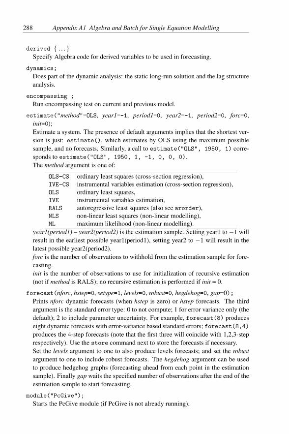
288 Appendix A1 Algebra and Batch for Single Equation Modelling
derived . . .Specify Algebra code for derived variables to be used in forecasting.
dynamics;
Does part of the dynamic analysis: the static long-run solution and the lag structureanalysis.
encompassing ;
Run encompassing test on current and previous model.
estimate("method"=OLS, year1=-1, period1=0, year2=-1, period2=0, forc=0,init=0);Estimate a system. The presence of default arguments implies that the shortest ver-sion is just: estimate(), which estimates by OLS using the maximum possiblesample, and no forecasts. Similarly, a call to estimate("OLS", 1950, 1) corre-sponds to estimate("OLS", 1950, 1, -1, 0, 0, 0).The method argument is one of:
OLS-CS ordinary least squares (cross-section regression),IVE-CS instrumental variables estimation (cross-section regression),OLS ordinary least squares,IVE instrumental variables estimation,RALS autoregressive least squares (also see arorder),NLS non-linear least squares (non-linear modelling),ML maximum likelihood (non-linear modelling).
year1(period1) – year2(period2) is the estimation sample. Setting year1 to −1 willresult in the earliest possible year1(period1), setting year2 to −1 will result in thelatest possible year2(period2).forc is the number of observations to withhold from the estimation sample for fore-casting.init is the number of observations to use for initialization of recursive estimation(not if method is RALS); no recursive estimation is performed if init = 0.
forecast(nforc, hstep=0, setype=1, levels=0, robust=0, hegdehog=0, gap=0);Prints nforc dynamic forecasts (when hstep is zero) or hstep forecasts. The thirdargument is the standard error type: 0 to not compute; 1 for error variance only (thedefault); 2 to include parameter uncertainty. For example, forecast(8) produceseight dynamic forecasts with error-variance based standard errors; forecast(8,4)produces the 4-step forecasts (note that the first three will coincide with 1,2,3-steprespectively). Use the store command next to store the forecasts if necessary.Set the levels argument to one to also produce levels forecasts; and set the robustargument to one to include robust forecasts. The hegdehog argument can be usedto produce hedgehog graphs (forecasting ahead from each point in the estimationsample). Finally gap waits the specified number of observations after the end of theestimation sample to start forecasting.
module("PcGive");
Starts the PcGive module (if PcGive is not already running).

A1.3 PcGive batch language 289
nonlinear . . .Formulates a non-linear model. The code between must conform to the syntaxof §A1.2.
output("option");Prints further output:
optioncorrelation print correlation matrix of variables,covariance print covariance matrix of coefficients,equation print the model equation format,forecasts print the static forecasts,HCSE Heteroscedasticity-consistent standard errorsinfcrit report information criteria,instability report instability tests,latex print the model in latex format,r2seasonals report R2 about seasonals,reducedform print the reduced form,sigpar significant digits for parameters (second argument),sigse significant digits for standard errors (second argument).
option("option", argument);The first set relates to maximization:
option argument valuemaxit maximum number of iterations default: 1000,print print every # iteration 0: do not print,compact compact or extended output 0 for off, 1 on,strong strong convergence tolerance default: 0.005,weak set weak convergence tolerance default: 0.0001,
The second set of options adds further output automatically:
option argument valueequation add equation format 0 for off, 1 on,infcrit report information criteria 0 for off, 1 on.instability report instability tests 0 for off, 1 on,HCSE Heteroscedasticity-consistent SEs 0 for off, 1 on,r2seasonals report R2 about seasonals 0 for off, 1 on,
package("PcGive", "package");Use this command to select the correct component (package) from PcGive:
package"Cross-section"
"Multiple-equation"
"Non-linear"
"Single-equation"
The package arguments can be shortened to 5 letters.
progress;

290 Appendix A1 Algebra and Batch for Single Equation Modelling
Reports the modelling progress.
store("name", "rename"="");Use this command to store residuals, etc. into the database, the default name isused. Note that if the variable already exists, it is overwritten without warning.The name must be one of: residuals, fitted, res1step, stdinn, rss, eqse,innov, loglik.The optional second argument replaces the default name. For exam-ple store("residuals") stores the residuals under the name Residual;store("residuals", "xyz") stores them under the name xyz.
system Y=. . . ; Z=. . . ; U=. . . ; A=. . . ; Specify the system, consisting of the following components:Y endogenous variables;A additional instruments (optional);Z non-modelled variables;U unrestricted variables (optional, treated as Z).
The variables listed are separated by commas, their base names (that is, name ex-cluding lag length) must be in the database. If the variable names are not a validtoken, the name must be enclosed in double quotes.The following special variables are recognized: Constant, Trend, Seasonal andCSeason.Note that when IVE/RIVE are used PcGive reorders the model as follows: the en-dogenous variables first and the additional instruments last. This reordering is rele-vant when specifying restrictions.
test("test", lag1=0, lag2=0);Performs a specific test using the specified lag lengths.
"ar" test for autocorrelated errors from lag1 to lag2;"arch" ARCH test up to order lag1;"comfac" test for common factor;"encompassing" tests the two most recent models for encompassing;"hetero" heteroscedasticity test (squares);"heterox" heteroscedasticity test (squares and cross products);"instability" instability tests;"normal" normality test;"rescor" residual correlogram up to lag lag1;"reset" Reset test using powers up to lag1.
testgenres . . .Used to test for general restrictions: specify the restrictions between , conform-ing to §A1.1.
testlinres . . .Test for linear restrictions. The content is the matrix dimensions followed by the(R : r) matrix.
testres . . .

A1.3 PcGive batch language 291
Test for exclusion restrictions. The content lists the variables to be tested for ex-clusion, separated by a comma (remember that variable names that are not propertokens must be enclosed in double quotes).
testsummary;
Do the test summary.
We finish with an annotated example using most commands. To run this file, weassume that OxMetrics is loaded with data.in7, and that PcGive has been started.
module("PcGive");package("PcGive", "Single-equation");usedata("data.in7");system
Y = CONS, INC; // endogenous variablesZ = CONS_1, INC_1, // non-modelled variables
Constant;A = OUTPUT, OUTPUT_1; // additional instruments, optional
estimate("IVE", 0, 0, 0, 0, 8);
// Estimate by IV over maximum sample:// 1953(2)-1992(3), use 8 forecasts
testsummary; // Do the test summary.dynamics; // Do dynamic analysis.store("residuals"); // store the residualstestgenres // Test for general restrictions.
&1 - &2 = 0; // coeff of CONS_1 - coeff of INC_1.testlinres // Test for linear restrictions. // same restriction
1 50 1 -1 0 0
testres // Test an exclusion restriction
CONS_1, INC_1
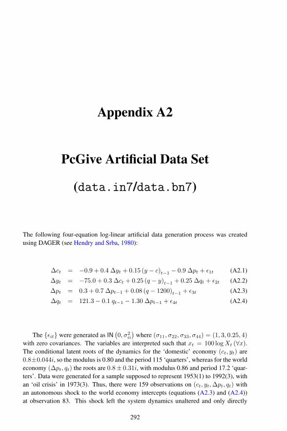
Appendix A2
PcGive Artificial Data Set
(data.in7/data.bn7)
The following four-equation log-linear artificial data generation process was createdusing DAGER (see Hendry and Srba, 1980):
∆ct = −0.9 + 0.4 ∆yt + 0.15 (y − c)t−1 − 0.9 ∆pt + ε1t (A2.1)
∆yt = −75.0 + 0.3 ∆ct + 0.25 (q − y)t−1 + 0.25 ∆qt + ε2t (A2.2)
∆pt = 0.3 + 0.7 ∆pt−1 + 0.08 (q − 1200)t−1 + ε3t (A2.3)
∆qt = 121.3− 0.1 qt−1 − 1.30 ∆pt−1 + ε4t (A2.4)
The εit were generated as IN(0, σ2
ii
)where (σ11, σ22, σ33, σ44) = (1, 3, 0.25, 4)
with zero covariances. The variables are interpreted such that xt = 100 logXt (∀x).The conditional latent roots of the dynamics for the ‘domestic’ economy (ct, yt) are0.8±0.044i, so the modulus is 0.80 and the period 115 ‘quarters’, whereas for the worldeconomy (∆pt, qt) the roots are 0.8± 0.31i, with modulus 0.86 and period 17.2 ‘quar-ters’. Data were generated for a sample supposed to represent 1953(1) to 1992(3), withan ‘oil crisis’ in 1973(3). Thus, there were 159 observations on (ct, yt,∆pt, qt) withan autonomous shock to the world economy intercepts (equations (A2.3) and (A2.4))at observation 83. This shock left the system dynamics unaltered and only directly
292

Appendix A2 PcGive Artificial Data Set (data.in7/data.bn7) 293
affected ∆pt and qt. The long-run equilibrium of the system was shifted from:
c = y − 6∆p− 6 [C = exp (−6∆p− 0.06)Y ]
y = q − 300 [Y = 0.05 Q]
with: ∆p = 1 [p = 1% per quarter]q = 1200 [Q = 162, 755]
to: ∆p = 2 [p = 2% per quarter]q = 1180 [Q = 133, 252]
Thus, ‘equilibrium’ inflation (p) doubled and world output fell by about 18%. Cor-rect modelling of the system necessitates different intercepts pre/post-1973(3) in equa-tions (A2.3) and (A2.4). The structural break was included so that issues of predictivefailure would be meaningful (see Hendry, 1979).
To ease recognition of the variables, they were respectively named CONS, INC,INFLAT and OUTPUT. Simultaneous equations estimation closely replicates these co-efficients of the DGP and the long-run solutions. Note that estimating (A2.2) by OLSyields a spectacular example of simultaneity bias and (A2.3) without the oil dummyshows massive predictive failure. Also, (A2.1) by RLS indicates evidence of parame-ter non-constancy owing to the change in the simultaneity bias at the oil crisis: mostmis-specifications also lead to predictive failure.

Appendix A3
Numerical Changes From PreviousVersions
A3.1 From version 12 to 13
• The degrees of freedom computation of some tests has changed:
PcGive ≤ 12 PcGive ≥ 13
ARCH test F(s, T − k − 2s) F(s, T − 2s)
Heteroscedasticity test F(s, T − s− 1− k) F(s, T − s− 1)
• Additional changes to the Heteroscedasticity test:– Observations that have a residual that is (almost) zero are removed.– When there are four or more equations, the vector Heteroscedasticity test is
based on the transformed residuals and omitting the cross-product. This keepsthe number of equations down to n (see Volume II).
– Unrestricted/fixed variables are now included in test (previously they were neverused in forming the squares or cross-products).
A3.2 From version 9 to 10
There are a only few minor changes: the RESET test now uses direct regression insteadof partioned inverse, resulting in small differences; the t-test for zero innovation meanis now implemented as in the documentation; NLS standard errors are now based on theinformation matrix; NLS AR test can be slightly different (as could the heteroscedas-ticity tests when degrees of freedom differ); RALS ARCH test degrees of freedom nowuse T after allowing for lagged residuals. The residual correlogram uses the more stan-dard textbook definition now (i.e. in deviation from the full sample mean, instead of therunning mean).
294

Appendix A3 Numerical Changes From Previous Versions 295
A3.3 From version 8 to 9The major change is the adoption of the QR decomposition with partial pivoting to com-pute OLS and IV estimates. There are also some minor improvements in accuracy, thefollowing tests are the most sensitive to such changes: encompassing, heteroscedastic-ity and RESET. The heteroscedasticity tests could also differ in the number of variablesremoved owing to singularity.
A3.4 From version 7 to 8The numerical results generated by PcGive version 8 are unchanged from version 7,apart from a marginal increase in accuracy of several diagnostic tests. Also, a newversion of the normality test is used now, which uses a small sample correction.


References
Ahumada, H. (1985). An encompassing test of two models of the balance of trade for Ar-gentina. Oxford Bulletin of Economics and Statistics 47, 51–70. [225]
Alexander, C. (2001). Market Models: A Guide to Financial Data Analysis. Chichester: JohnWiley and Sons. [240]
Amemiya, T. (1981). Qualitative response models: A survey. Journal of Economic Litera-ture 19, 1483–1536. [102]
Amemiya, T. (1985). Advanced Econometrics. Oxford: Basil Blackwell. [105]
Anderson, T. W. (1971). The Statistical Analysis of Time Series. New York: John Wiley &Sons. [177]
Andrews, D. W. K. (1991). Heteroskedasticity and autocorrelation consistent covariance ma-trix estimation. Econometrica 59, 817–858. [156, 250]
Baba, Y., D. F. Hendry, and R. M. Starr (1992). The demand for M1 in the U.S.A., 1960–1988.Review of Economic Studies 59, 25–61. [176, 228]
Banerjee, A., J. J. Dolado, J. W. Galbraith, and D. F. Hendry (1993). Co-integration, ErrorCorrection and the Econometric Analysis of Non-Stationary Data. Oxford: Oxford Uni-versity Press. [47, 63, 139, 143, 231, 239]
Banerjee, A., J. J. Dolado, D. F. Hendry, and G. W. Smith (1986). Exploring equilibriumrelationships in econometrics through static models: Some Monte Carlo evidence. OxfordBulletin of Economics and Statistics 48, 253–277. [145, 163]
Banerjee, A., J. J. Dolado, and R. Mestre (1998). Error-correction mechanism tests for coin-tegration in a single equation framework. Journal of Time Series Analysis 19, 267–283.[48]
Banerjee, A. and D. F. Hendry (Eds.) (1992). Testing Integration and Cointegration. OxfordBulletin of Economics and Statistics: 54. [139, 239]
Banerjee, A. and D. F. Hendry (1992). Testing integration and cointegration: An overview.Oxford Bulletin of Economics and Statistics 54, 225–255. [158]
Bardsen, G. (1989). The estimation of long run coefficients from error correction models.Oxford Bulletin of Economics and Statistics 50. [267]
Bentzel, R. and B. Hansen (1955). On recursiveness and interdependency in economic models.Review of Economic Studies 22, 153–168. [152]
Bollerslev, T., R. S. Chou, and K. F. Kroner (1992). ARCH modelling in finance – A reviewof the theory and empirical evidence. Journal of Econometrics 52, 5–59. [110]
Bontemps, C. and G. E. Mizon (2003). Congruence and encompassing. In B. P. Stigum (Ed.),Econometrics and the Philosophy of Economics, pp. 354–378. Princeton: Princeton Uni-versity Press. [171, 213]
297

298 REFERENCES
Bowman, K. O. and L. R. Shenton (1975). Omnibus test contours for departures from normal-ity based on
√b1 and b2. Biometrika 62, 243–250. [276]
Box, G. E. P. and G. M. Jenkins (1976). Time Series Analysis, Forecasting and Control. SanFrancisco: Holden-Day. First published, 1970. [108, 145]
Box, G. E. P. and D. A. Pierce (1970). Distribution of residual autocorrelations inautoregressive-integrated moving average time series models. Journal of the AmericanStatistical Association 65, 1509–1526. [274]
Breusch, T. S. and A. R. Pagan (1980). The Lagrange multiplier test and its applications tomodel specification in econometrics. Review of Economic Studies 47, 239–253. [209]
Brown, R. L., J. Durbin, and J. M. Evans (1975). Techniques for testing the constancy of re-gression relationships over time (with discussion). Journal of the Royal Statistical SocietyB 37, 149–192. [265]
Campos, J., N. R. Ericsson, and D. F. Hendry (1996). Cointegration tests in the presence ofstructural breaks. Journal of Econometrics 70, 187–220. [142]
Chambers, E. A. and D. R. Cox (1967). Discrimination between alternative binary responsemodels. Biometrika 54, 573–578. [104]
Chow, G. C. (1960). Tests of equality between sets of coefficients in two linear regressions.Econometrica 28, 591–605. [169, 200, 209, 211, 253, 265]
Clements, M. P. and D. F. Hendry (1998). Forecasting Economic Time Series. Cambridge:Cambridge University Press. [56, 146, 231, 269]
Clements, M. P. and D. F. Hendry (1999). Forecasting Non-stationary Economic Time Series.Cambridge, Mass.: MIT Press. [146, 231]
Clements, M. P. and D. F. Hendry (2011). Forecasting from misspecified models in the pres-ence of unanticipated location shifts. See Clements and Hendry (2011), pp. 271–314.[271]
Clements, M. P. and D. F. Hendry (Eds.) (2011). The Oxford Handbook of Economic Fore-casting. Oxford: Oxford University Press. [269, 298]
Cochrane, D. and G. H. Orcutt (1949). Application of least squares regression to relationshipscontaining auto-correlated error terms. Journal of the American Statistical Association 44,32–61. [147]
Cox, D. R. (1961). Tests of separate families of hypotheses. In Proceedings of the FourthBerkeley Symposium on Mathematical Statistics and Probability, Volume 1, Berkeley, pp.105–123. University of California Press. [171, 280]
Cramer, J. S. (1986). Econometric Applications of Maximum Likelihood Methods. Cambridge:Cambridge University Press. [105]
D’Agostino, R. B. (1970). Transformation to normality of the null distribution of g1.Biometrika 57, 679–681. [276]
Davidson, J. E. H., D. F. Hendry, F. Srba, and J. S. Yeo (1978). Econometric modelling ofthe aggregate time-series relationship between consumers’ expenditure and income in theUnited Kingdom. Economic Journal 88, 661–692. Reprinted in Hendry, D. F., Economet-rics: Alchemy or Science? Oxford: Blackwell Publishers, 1993, and Oxford UniversityPress, 2000; and in Campos, J., Ericsson, N.R. and Hendry, D.F. (eds.), General to SpecificModelling. Edward Elgar, 2005. [11, 59, 75, 76, 130, 142, 147, 149, 166, 224, 228]
Davidson, R. and J. G. MacKinnon (1993). Estimation and Inference in Econometrics. NewYork: Oxford University Press. [274]
Dickey, D. A. and W. A. Fuller (1981). Likelihood ratio statistics for autoregressive time serieswith a unit root. Econometrica 49, 1057–1072. [238]
REFERENCES 299
Doan, T., R. Litterman, and C. A. Sims (1984). Forecasting and conditional projection usingrealistic prior distributions. Econometric Reviews 3, 1–100. [146, 228]
Doornik, J. A. (2007). Autometrics. Mimeo, Department of Economics, University of Oxford.[220]
Doornik, J. A. (2008). Encompassing and automatic model selection. Oxford Bulletin of Eco-nomics and Statistics 70, 915–925. [178]
Doornik, J. A. (2009). Autometrics. In J. L. Castle and N. Shephard (Eds.), The Methodologyand Practice of Econometrics: Festschrift in Honour of David F. Hendry. Oxford: OxfordUniversity Press. [178]
Doornik, J. A. (2013). Object-Oriented Matrix Programming using Ox (7th ed.). London:Timberlake Consultants Press. [4, 273]
Doornik, J. A. and H. Hansen (1994). A practical test for univariate and multivariate normality.Discussion paper, Nuffield College. [276]
Doornik, J. A. and D. F. Hendry (1992). PCGIVE 7: An Interactive Econometric ModellingSystem. Oxford: Institute of Economics and Statistics, University of Oxford. [3]
Doornik, J. A. and D. F. Hendry (1994). PcGive 8: An Interactive Econometric ModellingSystem. London: International Thomson Publishing, and Belmont, CA: Duxbury Press.[3]
Doornik, J. A. and D. F. Hendry (2013a). Econometric Modelling using PcGive: Volume III(4th ed.). London: Timberlake Consultants Press. [100]
Doornik, J. A. and D. F. Hendry (2013b). Interactive Monte Carlo Experimentation in Econo-metrics Using PcNaive (3rd ed.). London: Timberlake Consultants Press. [135]
Doornik, J. A. and D. F. Hendry (2013c). Modelling Dynamic Systems using PcGive: VolumeII (5th ed.). London: Timberlake Consultants Press. [115, 135, 201, 251, 269]
Doornik, J. A. and D. F. Hendry (2013d). OxMetrics: An Interface to Empirical Modelling(7th ed.). London: Timberlake Consultants Press. [4]
Doornik, J. A. and M. Ooms (2006). Introduction to Ox (2nd ed.). London: Timberlake Con-sultants Press. [97]
Durbin, J. (1970). Testing for serial correlation in least squares regression when some of theregressors are lagged dependent variables. Econometrica 38, 410–421. [275]
Eicker, F. (1967). Limit theorems for regressions with unequal and dependent errors. In Pro-ceedings of the Fifth Berkeley Symposium on Mathematical Statistics and Probability,Volume 1, Berkeley, pp. 59–82. University of California. [155]
Eisner, R. and R. H. Strotz (1963). Determinants of Business Investment. Englewood Cliffs,N.J.: Prentice-Hall. [147]
Emerson, R. A. and D. F. Hendry (1996). An evaluation of forecasting using leading indicators.Journal of Forecasting 15, 271–291. Reprinted in T.C. Mills (ed.), Economic Forecasting.Edward Elgar, 1999. [146]
Engle, R. F. (1982). Autoregressive conditional heteroscedasticity, with estimates of the vari-ance of United Kingdom inflation. Econometrica 50, 987–1007. [110, 158, 210, 277, 278]
Engle, R. F. (1984). Wald, likelihood ratio, and Lagrange multiplier tests in econometrics. SeeGriliches and Intriligator (1984), Chapter 13. [209, 211]
Engle, R. F. and C. W. J. Granger (1987). Cointegration and error correction: Representation,estimation and testing. Econometrica 55, 251–276. [139, 145, 149, 163, 178, 231]
Engle, R. F., D. F. Hendry, and J.-F. Richard (1983). Exogeneity. Econometrica 51, 277–304. Reprinted in Hendry, D. F., Econometrics: Alchemy or Science? Oxford: BlackwellPublishers, 1993, and Oxford University Press, 2000; in Ericsson, N. R. and Irons, J. S.

300 REFERENCES
(eds.) Testing Exogeneity, Oxford: Oxford University Press, 1994; and in Campos, J.,Ericsson, N.R. and Hendry, D.F. (eds.), General to Specific Modelling. Edward Elgar,2005. [142, 144, 167, 204, 205, 211, 214]
Engle, R. F., D. F. Hendry, and D. Trumbull (1985). Small sample properties of ARCH esti-mators and tests. Canadian Journal of Economics 43, 66–93. [158, 278]
Engle, R. F. and H. White (Eds.) (1999). Cointegration, Causality and Forecasting. Oxford:Oxford University Press. [303, 307]
Engler, E. and B. Nielsen (2009). The empirical process of autoregressive residuals. Econo-metrics Journal 12, 367–381. [243]
Ericsson, N. R. (1983). Asymptotic properties of instrumental variables statistics for testingnon-nested hypotheses. Review of Economic Studies 50, 287–303. [171, 280]
Ericsson, N. R. (1992). Cointegration, exogeneity and policy analysis: An overview. Journalof Policy Modeling 14, 251–280. [206]
Ericsson, N. R. and D. F. Hendry (1999). Encompassing and rational expectations: How se-quential corroboration can imply refutation. Empirical Economics 24, 1–21. [176]
Ericsson, N. R. and J. S. Irons (1995). The Lucas critique in practice: Theory without measure-ment. In K. D. Hoover (Ed.), Macroeconometrics: Developments, Tensions and Prospects,pp. 263–312. Dordrecht: Kluwer Academic Press. [145]
Ericsson, N. R. and J. G. MacKinnon (2002). Distributions of error correction tests for coin-tegration. Econometrics Journal 5, 285–318. [267]
Escribano, A. (1985). Non-linear error correction: The case of money demand in the UK(1878–1970). Mimeo, University of California at San Diego. [149]
Favero, C. and D. F. Hendry (1992). Testing the Lucas critique: A review. Econometric Re-views 11, 265–306. [145, 211, 226]
Finney, D. J. (1947). The estimation from individual records of the relationship between doseand quantal response. Biometrika 34, 320–334. [100, 101]
Fletcher, R. (1987). Practical Methods of Optimization, (2nd ed.). New York: John Wiley &Sons. [99]
Friedman, M. and A. J. Schwartz (1982). Monetary Trends in the United States and the UnitedKingdom: Their Relation to Income, Prices, and Interest Rates, 1867–1975. Chicago:University of Chicago Press. [216]
Frisch, R. (1934). Statistical Confluence Analysis by means of Complete Regression Systems.Oslo: University Institute of Economics. [222]
Frisch, R. (1938). Statistical versus theoretical relations in economic macrodynamics. Mimeo-graph dated 17 July 1938, League of Nations Memorandum. Reproduced by University ofOslo in 1948 with Tinbergen’s comments. Contained in Memorandum ‘Autonomy of Eco-nomic Relations’, 6 November 1948, Oslo, Universitets Økonomiske Institutt. Reprintedin Hendry D. F. and Morgan M. S. (1995), The Foundations of Econometric Analysis.Cambridge: Cambridge University Press. [152]
Frisch, R. and F. V. Waugh (1933). Partial time regression as compared with individual trends.Econometrica 1, 221–223. [195]
Gilbert, C. L. (1986). Professor Hendry’s econometric methodology. Oxford Bulletin of Eco-nomics and Statistics 48, 283–307. Reprinted in Granger, C. W. J. (ed.) (1990), ModellingEconomic Series. Oxford: Clarendon Press. [210, 232]
Gilbert, C. L. (1989). LSE and the British approach to time-series econometrics. Oxford Re-view of Economic Policy 41, 108–128. [147]
Godfrey, L. G. (1978). Testing for higher order serial correlation in regression equations whenthe regressors include lagged dependent variables. Econometrica 46, 1303–1313. [275]

REFERENCES 301
Godfrey, L. G. (1988). Misspecification Tests in Econometrics. Cambridge: Cambridge Uni-versity Press. [173, 209]
Godfrey, L. G. and C. D. Orme (1994). The sensitivity of some general checks to omittedvariables in the linear model. International Economic Review 35, 489–506. [277]
Golub, G. H. and C. F. Van Loan (1989). Matrix Computations. Baltimore: The Johns HopkinsUniversity Press. [241]
Granger, C. W. J. (1969). Investigating causal relations by econometric models and cross-spectral methods. Econometrica 37, 424–438. [175]
Granger, C. W. J. (1986). Developments in the study of cointegrated economic variables. Ox-ford Bulletin of Economics and Statistics 48, 213–228. [139, 231]
Granger, C. W. J. and P. Newbold (1974). Spurious regressions in econometrics. Journal ofEconometrics 2, 111–120. [145]
Granger, C. W. J. and P. Newbold (1977). The time series approach to econometric modelbuilding. In C. A. Sims (Ed.), New Methods in Business Cycle Research, pp. 7–21. Min-neapolis: Federal Reserve Bank of Minneapolis. [146]
Granger, C. W. J. and P. Newbold (1986). Forecasting Economic Time Series, (2nd ed.). NewYork: Academic Press. [242]
Gregory, A. W. and M. R. Veale (1985). Formulating Wald tests of non-linear restrictions.Econometrica 53, 1465–1468. [160]
Griliches, Z. and M. D. Intriligator (Eds.) (1984). Handbook of Econometrics, Volume 2.Amsterdam: North-Holland. [209, 299, 303]
Hansen, B. E. (1992). Testing for parameter instability in linear models. Journal of PolicyModeling 14, 517–533. [78, 209, 211, 278]
Harvey, A. C. (1981). The Econometric Analysis of Time Series. Deddington: Philip Allan.[209]
Harvey, A. C. (1990). The Econometric Analysis of Time Series, (2nd ed.). Hemel Hempstead:Philip Allan. [209, 273, 275]
Harvey, A. C. (1993). Time Series Models, (2nd ed.). Hemel Hempstead: Harvester Wheat-sheaf. [108, 241]
Harvey, A. C. and P. Collier (1977). Testing for functional misspecification in regression anal-ysis. Journal of Econometrics 6, 103–119. [253]
Harvey, A. C. and N. G. Shephard (1992). Structural time series models. In G. S. Maddala,C. R. Rao, and H. D. Vinod (Eds.), Handbook of Statistics, Volume 11. Amsterdam:North-Holland. [229]
Hendry, D. F. (1976). The structure of simultaneous equations estimators. Journal of Econo-metrics 4, 51–88. Reprinted in Hendry, D. F., Econometrics: Alchemy or Science? Oxford:Blackwell Publishers, 1993, and Oxford University Press, 2000. [206, 256]
Hendry, D. F. (1979). Predictive failure and econometric modelling in macro-economics: Thetransactions demand for money. In P. Ormerod (Ed.), Economic Modelling, pp. 217–242.London: Heinemann. Reprinted in Hendry, D. F., Econometrics: Alchemy or Science?Oxford: Blackwell Publishers, 1993, and Oxford University Press, 2000; and in Campos,J., Ericsson, N.R. and Hendry, D.F. (eds.), General to Specific Modelling. Edward Elgar,2005. [215, 228, 293]
Hendry, D. F. (1980). Econometrics: Alchemy or science? Economica 47, 387–406. Reprintedin Hendry, D. F., Econometrics: Alchemy or Science? Oxford: Blackwell Publishers,1993, and Oxford University Press, 2000. [134, 207, 232]
Hendry, D. F. (Ed.) (1986). Econometric Modelling with Cointegrated Variables. Oxford Bul-letin of Economics and Statistics: 48. [239]

302 REFERENCES
Hendry, D. F. (1986a). Econometric modelling with cointegrated variables: An overview.Oxford Bulletin of Economics and Statistics 48, 201–212. Reprinted in R.F. Engle andC.W.J. Granger (eds), Long-Run Economic Relationships, Oxford: Oxford UniversityPress, 1991, 51–63. [139]
Hendry, D. F. (1986b). Using PC-GIVE in econometrics teaching. Oxford Bulletin of Eco-nomics and Statistics 48, 87–98. [3, 216]
Hendry, D. F. (1987). Econometric methodology: A personal perspective. In T. F. Bewley(Ed.), Advances in Econometrics, pp. 29–48. Cambridge: Cambridge University Press.Reprinted in Campos, J., Ericsson, N.R. and Hendry, D.F. (eds.), General to SpecificModelling. Edward Elgar, 2005. [60, 178, 208, 214, 216]
Hendry, D. F. (1988). The encompassing implications of feedback versus feedforward mech-anisms in econometrics. Oxford Economic Papers 40, 132–149. Reprinted in Ericsson,N. R. and Irons, J. S. (eds.) Testing Exogeneity, Oxford: Oxford University Press, 1994;and in Campos, J., Ericsson, N.R. and Hendry, D.F. (eds.), General to Specific Modelling.Edward Elgar, 2005. [169, 178, 211, 226, 228]
Hendry, D. F. (1989). Comment on intertemporal consumer behaviour under structuralchanges in income. Econometric Reviews 8, 111–121. [232]
Hendry, D. F. (1993). Econometrics: Alchemy or Science? Oxford: Blackwell Publishers. [3,8, 116, 178]
Hendry, D. F. (1995a). Dynamic Econometrics. Oxford: Oxford University Press. [8, 11, 116,134, 139, 148, 167, 183, 206, 209, 212, 213, 216, 229]
Hendry, D. F. (1995b). On the interactions of unit roots and exogeneity. Econometric Re-views 14, 383–419. [211]
Hendry, D. F. (1995c). A theory of co-breaking. Mimeo, Nuffield College, University of Ox-ford. [231]
Hendry, D. F. (1996). On the constancy of time-series econometric equations. Economic andSocial Review 27, 401–422. [229]
Hendry, D. F. (1997). On congruent econometric relations: A comment. Carnegie–RochesterConference Series on Public Policy 47, 163–190. [226]
Hendry, D. F. (2000a). Econometrics: Alchemy or Science? Oxford: Oxford University Press.New Edition. [116, 178, 302]
Hendry, D. F. (2000b). Epilogue: The success of general-to-specific model selection. SeeHendry (2000a), pp. 467–490. New Edition. [178]
Hendry, D. F. and G. J. Anderson (1977). Testing dynamic specification in small simultaneoussystems: An application to a model of building society behaviour in the United Kingdom.In M. D. Intriligator (Ed.), Frontiers in Quantitative Economics, Volume 3, pp. 361–383.Amsterdam: North Holland Publishing Company. Reprinted in Hendry, D. F., Economet-rics: Alchemy or Science? Oxford: Blackwell Publishers, 1993, and Oxford UniversityPress, 2000. [146, 149]
Hendry, D. F. and J. A. Doornik (1994). Modelling linear dynamic econometric systems. Scot-tish Journal of Political Economy 41, 1–33. [178]
Hendry, D. F. and J. A. Doornik (1997). The implications for econometric modelling of fore-cast failure. Scottish Journal of Political Economy 44, 437–461. Special Issue. [229]
Hendry, D. F. and N. R. Ericsson (1991). Modeling the demand for narrow money in the UnitedKingdom and the United States. European Economic Review 35, 833–886. [8, 228]
Hendry, D. F., S. Johansen, and C. Santos (2004). Selecting a regression saturated by indica-tors. Unpublished paper, Economics Department, University of Oxford. [234]

REFERENCES 303
Hendry, D. F. and K. Juselius (2000). Explaining cointegration analysis: Part I. Energy Jour-nal 21, 1–42. [136, 141]
Hendry, D. F. and H.-M. Krolzig (1999). Improving on ‘Data mining reconsidered’ by K.D.Hoover and S.J. Perez. Econometrics Journal 2, 202–219. Reprinted in J. Campos, N.R.Ericsson and D.F. Hendry (eds.), General to Specific Modelling. Edward Elgar, 2005.[178, 220, 221, 233]
Hendry, D. F. and H.-M. Krolzig (2001). Automatic Econometric Model Selection. London:Timberlake Consultants Press. [220]
Hendry, D. F. and H.-M. Krolzig (2005). The properties of automatic Gets modelling. Eco-nomic Journal 115, C32–C61. [218, 233]
Hendry, D. F. and M. Massmann (2007). Co-breaking: Recent advances and a synopsis of theliterature. Journal of Business and Economic Statistics 25, 33–51. [231]
Hendry, D. F. and G. E. Mizon (1978). Serial correlation as a convenient simplification, nota nuisance: A comment on a study of the demand for money by the Bank of England.Economic Journal 88, 549–563. Reprinted in Hendry, D. F., Econometrics: Alchemy orScience? Oxford: Blackwell Publishers, 1993, and Oxford University Press, 2000; andin Campos, J., Ericsson, N.R. and Hendry, D.F. (eds.), General to Specific Modelling.Edward Elgar, 2005. [52, 148, 216, 224, 268]
Hendry, D. F. and G. E. Mizon (1993). Evaluating dynamic econometric models by encom-passing the VAR. In P. C. B. Phillips (Ed.), Models, Methods and Applications of Econo-metrics, pp. 272–300. Oxford: Basil Blackwell. Reprinted in Campos, J., Ericsson, N.R.and Hendry, D.F. (eds.), General to Specific Modelling. Edward Elgar, 2005. [145, 150,203, 214, 227]
Hendry, D. F. and G. E. Mizon (1999). The pervasiveness of Granger causality in economet-rics. See Engle and White (1999), pp. 102–134. [175]
Hendry, D. F. and M. S. Morgan (1989). A re-analysis of confluence analysis. Oxford Eco-nomic Papers 41, 35–52. [222]
Hendry, D. F. and M. S. Morgan (1995). The Foundations of Econometric Analysis. Cam-bridge: Cambridge University Press. [11, 134]
Hendry, D. F. and A. J. Neale (1987). Monte Carlo experimentation using PC-NAIVE. InT. Fomby and G. F. Rhodes (Eds.), Advances in Econometrics, Volume 6, pp. 91–125.Greenwich, Connecticut: Jai Press Inc. [135, 200, 207, 211]
Hendry, D. F. and A. J. Neale (1988). Interpreting long-run equilibrium solutions in conven-tional macro models: A comment. Economic Journal 98, 808–817. [226]
Hendry, D. F. and A. J. Neale (1991). A Monte Carlo study of the effects of structural breaks ontests for unit roots. In P. Hackl and A. H. Westlund (Eds.), Economic Structural Change,Analysis and Forecasting, pp. 95–119. Berlin: Springer-Verlag. [231]
Hendry, D. F., A. J. Neale, and N. R. Ericsson (1991). PC-NAIVE, An Interactive Programfor Monte Carlo Experimentation in Econometrics. Version 6.0. Oxford: Institute of Eco-nomics and Statistics, University of Oxford. [135, 178]
Hendry, D. F., A. J. Neale, and F. Srba (1988). Econometric analysis of small linear systemsusing Pc-Fiml. Journal of Econometrics 38, 203–226. [178, 202, 203, 206, 228]
Hendry, D. F. and B. Nielsen (2007). Econometric Modeling: A Likelihood Approach. Prince-ton: Princeton University Press. [11, 117]
Hendry, D. F., A. R. Pagan, and J. D. Sargan (1984). Dynamic specification. See Griliches andIntriligator (1984), pp. 1023–1100. Reprinted in Hendry, D. F., Econometrics: Alchemyor Science? Oxford: Blackwell Publishers, 1993, and Oxford University Press, 2000;

304 REFERENCES
and in Campos, J., Ericsson, N.R. and Hendry, D.F. (eds.), General to Specific Modelling.Edward Elgar, 2005. [143, 149, 151, 268]
Hendry, D. F. and J.-F. Richard (1982). On the formulation of empirical models in dynamiceconometrics. Journal of Econometrics 20, 3–33. Reprinted in Granger, C. W. J. (ed.)(1990), Modelling Economic Series. Oxford: Clarendon Press and in Hendry D. F., Econo-metrics: Alchemy or Science? Oxford: Blackwell Publishers 1993, and Oxford UniversityPress, 2000; and in Campos, J., Ericsson, N.R. and Hendry, D.F. (eds.), General to SpecificModelling. Edward Elgar, 2005. [171, 210, 213, 214]
Hendry, D. F. and J.-F. Richard (1983). The econometric analysis of economic time series(with discussion). International Statistical Review 51, 111–163. Reprinted in Hendry,D. F., Econometrics: Alchemy or Science? Oxford: Blackwell Publishers, 1993, andOxford University Press, 2000. [152, 178, 210, 225]
Hendry, D. F. and J.-F. Richard (1989). Recent developments in the theory of encompassing. InB. Cornet and H. Tulkens (Eds.), Contributions to Operations Research and Economics.The XXth Anniversary of CORE, pp. 393–440. Cambridge, MA: MIT Press. Reprintedin Campos, J., Ericsson, N.R. and Hendry, D.F. (eds.), General to Specific Modelling.Edward Elgar, 2005. [171, 213, 225, 280]
Hendry, D. F. and F. Srba (1980). AUTOREG: A computer program library for dynamic econo-metric models with autoregressive errors. Journal of Econometrics 12, 85–102. Reprintedin Hendry, D. F., Econometrics: Alchemy or Science? Oxford: Blackwell Publishers,1993, and Oxford University Press, 2000. [3, 292]
Hendry, D. F. and T. von Ungern-Sternberg (1981). Liquidity and inflation effects on con-sumers’ expenditure. In A. S. Deaton (Ed.), Essays in the Theory and Measurement ofConsumers’ Behaviour, pp. 237–261. Cambridge: Cambridge University Press. Reprintedin Hendry, D. F., Econometrics: Alchemy or Science? Oxford: Blackwell Publishers,1993, and Oxford University Press, 2000. [166]
Hendry, D. F. and K. F. Wallis (Eds.) (1984). Econometrics and Quantitative Economics.Oxford: Basil Blackwell. [305, 306]
Hooker, R. H. (1901). Correlation of the marriage rate with trade. Journal of the Royal Sta-tistical Society 64, 485–492. Reprinted in Hendry, D. F. and Morgan, M. S. (1995), TheFoundations of Econometric Analysis. Cambridge: Cambridge University Press. [126]
Hoover, K. D. and S. J. Perez (1999). Data mining reconsidered: Encompassing and thegeneral-to-specific approach to specification search. Econometrics Journal 2, 167–191.[116, 178, 220, 233]
Jarque, C. M. and A. K. Bera (1987). A test for normality of observations and regressionresiduals. International Statistical Review 55, 163–172. [276]
Johansen, S. (1988). Statistical analysis of cointegration vectors. Journal of Economic Dynam-ics and Control 12, 231–254. Reprinted in R.F. Engle and C.W.J. Granger (eds), Long-RunEconomic Relationships, Oxford: Oxford University Press, 1991, 131–52. [178, 203, 231]
Johansen, S. (1995). Likelihood-based Inference in Cointegrated Vector Autoregressive Mod-els. Oxford: Oxford University Press. [47, 139]
Johansen, S. and K. Juselius (1990). Maximum likelihood estimation and inference on coin-tegration – With application to the demand for money. Oxford Bulletin of Economics andStatistics 52, 169–210. [203]
Johnson, N. L. (1949). Systems of frequency curves generated by methods of translation.Biometrika 36, 149–176. [272]
Judd, J. and J. Scadding (1982). The search for a stable money demand function: A survey ofthe post-1973 literature. Journal of Economic Literature 20, 993–1023. [228]

REFERENCES 305
Judge, G. G., W. E. Griffiths, R. C. Hill, H. Lutkepohl, and T.-C. Lee (1985). The Theory andPractice of Econometrics, (2nd ed.). New York: John Wiley. [205, 247, 250]
Kiviet, J. F. (1986). On the rigor of some mis-specification tests for modelling dynamic rela-tionships. Review of Economic Studies 53, 241–261. [252, 273]
Kiviet, J. F. (1987). Testing Linear Econometric Models. Amsterdam: University of Amster-dam. [209]
Kiviet, J. F. and G. D. A. Phillips (1992). Exact similar tests for unit roots and cointegration.Oxford Bulletin of Economics and Statistics 54, 349–367. [143, 239]
Kohn, A. (1987). False Prophets. Oxford: Basil Blackwell. [232]Koopmans, T. C. (Ed.) (1950). Statistical Inference in Dynamic Economic Models. Number 10
in Cowles Commission Monograph. New York: John Wiley & Sons. [26, 305]Koopmans, T. C., H. Rubin, and R. B. Leipnik (1950). Measuring the equation systems of
dynamic economics. See Koopmans (1950), Chapter 2. [227]Kremers, J. J. M., N. R. Ericsson, and J. J. Dolado (1992). The power of cointegration tests.
Oxford Bulletin of Economics and Statistics 54, 325–348. [142]Kuh, E., D. A. Belsley, and R. E. Welsh (1980). Regression Diagnostics. Identifying Influential
Data and Sources of Collinearity. Wiley Series in Probability and Mathematical Statistics.New York: John Wiley. [223]
Leamer, E. E. (1978). Specification Searches. Ad-Hoc Inference with Non-Experimental Data.New York: John Wiley. [231]
Leamer, E. E. (1983). Let’s take the con out of econometrics. American Economic Review 73,31–43. Reprinted in Granger, C. W. J. (ed.) (1990), Modelling Economic Series. Oxford:Clarendon Press. [223]
Ljung, G. M. and G. E. P. Box (1978). On a measure of lack of fit in time series models.Biometrika 65, 297–303. [274]
Lovell, M. C. (1983). Data mining. Review of Economics and Statistics 65, 1–12. [220, 233]Lucas, R. E. (1976). Econometric policy evaluation: A critique. In K. Brunner and A. Meltzer
(Eds.), The Phillips Curve and Labor Markets, Volume 1 of Carnegie-Rochester Con-ferences on Public Policy, pp. 19–46. Amsterdam: North-Holland Publishing Company.[145, 228]
MacKinnon, J. G. (1991). Critical values for cointegration tests. In R. F. Engle and C. W. J.Granger (Eds.), Long-Run Economic Relationships, pp. 267–276. Oxford: Oxford Uni-versity Press. [38, 239]
MacKinnon, J. G. and H. White (1985). Some heteroskedasticity-consistent covariance matrixestimators with improved finite sample properties. Journal of Econometrics 29, 305–325.[156, 210, 250]
Makridakis, S., S. C. Wheelwright, and R. C. Hyndman (1998). Forecasting: Methods andApplications (3rd ed.). New York: John Wiley and Sons. [56]
Marschak, J. (1953). Economic measurements for policy and prediction. In W. C. Hood andT. C. Koopmans (Eds.), Studies in Econometric Method, Number 14 in Cowles Commis-sion Monograph. New York: John Wiley & Sons. [152]
Mizon, G. E. (1977). Model selection procedures. In M. J. Artis and A. R. Nobay (Eds.),Studies in Modern Economic Analysis, pp. 97–120. Oxford: Basil Blackwell. [216]
Mizon, G. E. (1984). The encompassing approach in econometrics. See Hendry and Wallis(1984), pp. 135–172. [171, 213, 280]
Mizon, G. E. (1995). A simple message for autocorrelation correctors: Don’t. Journal ofEconometrics 69, 267–288. [149]

306 REFERENCES
Mizon, G. E. and D. F. Hendry (1980). An empirical application and Monte Carlo analysisof tests of dynamic specification. Review of Economic Studies 49, 21–45. Reprinted inHendry, D. F., Econometrics: Alchemy or Science? Oxford: Blackwell Publishers, 1993,and Oxford University Press, 2000. [268]
Mizon, G. E. and J.-F. Richard (1986). The encompassing principle and its application tonon-nested hypothesis tests. Econometrica 54, 657–678. [171, 213, 280]
Nelson, C. R. (1972). The prediction performance of the FRB-MIT-PENN model of the USeconomy. American Economic Review 62, 902–917. Reprinted in T.C. Mills (ed.), Eco-nomic Forecasting. Edward Elgar, 1999. [146]
Newey, W. K. and K. D. West (1987). A simple positive semi-definite heteroskedasticity andautocorrelation-consistent covariance matrix. Econometrica 55, 703–708. [156, 250]
Nickell, S. J. (1985). Error correction, partial adjustment and all that: An expository note.Oxford Bulletin of Economics and Statistics 47, 119–130. [147]
Nielsen, B. (2006a). Correlograms for non-stationary autoregressions. Journal of the RoyalStatistical Society, B 68, 707–720. [241]
Nielsen, B. (2006b). Correlograms for non-stationary autoregressions. Journal of the RoyalStatistical Society B 68, 707–720. [274]
Pagan, A. R. (1984). Model evaluation by variable addition. See Hendry and Wallis (1984),pp. 103–135. [209, 275]
Perron, P. (1989). The Great Crash, the oil price shock and the unit root hypothesis. Econo-metrica 57, 1361–1401. [231]
Pesaran, M. H. (1974). On the general problem of model selection. Review of Economic Stud-ies 41, 153–171. Reprinted in Campos, J., Ericsson, N.R. and Hendry, D.F. (eds.), Generalto Specific Modelling. Edward Elgar, 2005. [171, 280]
Phillips, P. C. B. (1986). Understanding spurious regressions in econometrics. Journal ofEconometrics 33, 311–340. [145]
Phillips, P. C. B. (1987). Time series regression with a unit root. Econometrica 55, 277–301.[178]
Phillips, P. C. B. (1991). Optimal inference in cointegrated systems. Econometrica 59, 283–306. [203, 231]
Poincare, H. (1905). Science and Hypothesis. New York: Science Press. [216]Priestley, M. B. (1981). Spectral Analysis and Time Series. London: Academic Press. [242]Ramsey, J. B. (1969). Tests for specification errors in classical linear least squares regression
analysis. Journal of the Royal Statistical Society B 31, 350–371. [278]Richard, J.-F. (1980). Models with several regimes and changes in exogeneity. Review of Eco-
nomic Studies 47, 1–20. [151]Sargan, J. D. (1958). The estimation of economic relationships using instrumental variables.
Econometrica 26, 393–415. [173]Sargan, J. D. (1959). The estimation of relationships with autocorrelated residuals by the use
of instrumental variables. Journal of the Royal Statistical Society B 21, 91–105. Reprintedas pp. 87–104 in Sargan J. D. (1988), Contributions to Econometrics, Vol. 1, Cambridge:Cambridge University Press. [171]
Sargan, J. D. (1964). Wages and prices in the United Kingdom: A study in econometricmethodology (with discussion). In P. E. Hart, G. Mills, and J. K. Whitaker (Eds.), Econo-metric Analysis for National Economic Planning, Volume 16 of Colston Papers, pp. 25–63. London: Butterworth Co. Reprinted as pp. 275–314 in Hendry D. F. and Wallis K. F.(eds.) (1984). Econometrics and Quantitative Economics. Oxford: Basil Blackwell, and

REFERENCES 307
as pp. 124–169 in Sargan J. D. (1988), Contributions to Econometrics, Vol. 1, Cambridge:Cambridge University Press. [82, 149, 210, 255]
Sargan, J. D. (1980a). The consumer price equation in the post-war British economy. Anexercise in equation specification testing. Review of Economic Studies 47, 113–135. [210]
Sargan, J. D. (1980b). Some tests of dynamic specification for a single equation. Economet-rica 48, 879–897. Reprinted as pp. 191–212 in Sargan J. D. (1988), Contributions toEconometrics, Vol. 1, Cambridge: Cambridge University Press. [139, 149, 224, 268]
Shenton, L. R. and K. O. Bowman (1977). A bivariate model for the distribution of√b1 and
b2. Journal of the American Statistical Association 72, 206–211. [276]Silverman, B. W. (1986). Density Estimation for Statistics and Data Analysis. London: Chap-
man and Hall. [243]Sims, C. A. (1980). Macroeconomics and reality. Econometrica 48, 1–48. Reprinted in
Granger, C. W. J. (ed.) (1990), Modelling Economic Series. Oxford: Clarendon Press.[145, 204, 214, 226, 227, 228]
Sims, C. A., J. H. Stock, and M. W. Watson (1990). Inference in linear time series models withsome unit roots. Econometrica 58, 113–144. [218]
Spanos, A. (1986). Statistical Foundations of Econometric Modelling. Cambridge: CambridgeUniversity Press. [177, 209, 212]
Wallis, K. F. (1987). Time series analysis of bounded economic variables. Journal of TimeSeries Analysis 8, 115–123. [272]
White, H. (1980). A heteroskedastic-consistent covariance matrix estimator and a direct testfor heteroskedasticity. Econometrica 48, 817–838. [152, 155, 156, 210, 250, 277]
White, H. (1984). Asymptotic Theory for Econometricians. London: Academic Press. [172,203]
White, H. (1990). A consistent model selection. In C. W. J. Granger (Ed.), Modelling Eco-nomic Series, pp. 369–383. Oxford: Clarendon Press. [213]
Wooldridge, J. M. (1999). Asymptotic properties of some specification tests in linear modelswith integrated processes. See Engle and White (1999), pp. 366–384. [218]
Working, E. J. (1927). What do statistical demand curves show? Quarterly Journal of Eco-nomics 41, 212–235. [227]
Yule, G. U. (1926). Why do we sometimes get nonsense-correlations between time-series? Astudy in sampling and the nature of time series (with discussion). Journal of the RoyalStatistical Society 89, 1–64. Reprinted in Hendry, D. F. and Morgan, M. S. (1995), TheFoundations of Econometric Analysis. Cambridge: Cambridge University Press. [133,145]


Author Index
Ahumada, H. 225Alexander, C. 240Amemiya, T. 102, 105Anderson, G. J. 146, 149Anderson, T. W. 177Andrews, D. W. K. 156, 250
Baba, Y. 176, 228Banerjee, A. 47, 48, 63, 139, 143, 145, 158,
163, 231, 239Belsley, D. A. 223Bentzel, R. 152Bera, A. K. 276Bollerslev, T. 110Bontemps, C. 171, 213Bowman, K. O. 276Box, G. E. P. 108, 145, 274Breusch, T. S. 209Brown, R. L. 265Bardsen, G. 267
Campos, J. 142Chambers, E. A. 104Chou, R. S. 110Chow, G. C. 169, 200, 209, 211, 253, 265Clements, M. P. 56, 146, 231, 269, 271Cochrane, D. 147Collier, P. 253Cox, D. R. 104, 171, 280Cramer, J. S. 105
D’Agostino, R. B. 276Davidson, J. E. H. 11, 59, 75, 76, 130, 142,
147, 149, 166, 224, 228Davidson, R. 274Dickey, D. A. 238Doan, T. 146, 228Dolado, J. J. 47, 48, 63, 139, 142, 143, 145,
163, 231, 239Doornik, J. A. 3, 4, 97, 100, 115, 135, 178,
201, 220, 229, 251, 269, 273, 276Durbin, J. 265, 275
Eicker, F. 155Eisner, R. 147
Emerson, R. A. 146Engle, R. F. 110, 139, 142, 144, 145, 149,
158, 163, 167, 178, 204, 205,209–211, 214, 231, 277, 278
Engler, E. 243Ericsson, N. R. 8, 135, 142, 145, 171, 176,
178, 206, 228, 267, 280Escribano, A. 149Evans, J. M. 265
Favero, C. 145, 211, 226Finney, D. J. 100, 101Fletcher, R. 99Friedman, M. 216Frisch, R. 152, 195, 222Fuller, W. A. 238
Galbraith, J. W. 47, 63, 139, 143, 231, 239Gilbert, C. L. 147, 210, 232Godfrey, L. G. 173, 209, 275, 277Golub, G. H. 241Granger, C. W. J. 139, 145, 146, 149, 163,
175, 178, 231, 242Gregory, A. W. 160Griffiths, W. E. 205, 247, 250
Hansen, B. 152Hansen, B. E. 78, 209, 211, 278Hansen, H. 276Harvey, A. C. 108, 209, 229, 241, 253, 273,
275Hendry, D. F. 3, 4, 8, 11, 47, 52, 56, 59, 60,
63, 75, 76, 100, 115–117, 130,134–136, 139, 141–152, 158, 163,166, 167, 169, 171, 175, 176, 178,183, 200–216, 218, 220–222,224–229, 231–234, 239, 251, 256,268, 269, 271, 278, 280, 292, 293,302
Hill, R. C. 205, 247, 250Hooker, R. H. 126Hoover, K. D. 116, 178, 220, 233Hyndman, R. C. 56
Irons, J. S. 145
309

310 AUTHOR INDEX
Jarque, C. M. 276Jenkins, G. M. 108, 145Johansen, S. 47, 139, 178, 203, 231, 234Johnson, N. L. 272Judd, J. 228Judge, G. G. 205, 247, 250Juselius, K. 136, 141, 203
Kiviet, J. F. 143, 209, 239, 252, 273Kohn, A. 232Koopmans, T. C. 227Kremers, J. J. M. 142Krolzig, H.-M. 178, 218, 220, 221, 233Kroner, K. F. 110Kuh, E. 223
Leamer, E. E. 223, 231Lee, T.-C. 205, 247, 250Leipnik, R. B. 227Litterman, R. 146, 228Ljung, G. M. 274Lovell, M. C. 220, 233Lucas, R. E. 145, 228Lutkepohl, H. 205, 247, 250
MacKinnon, J. G. 38, 156, 210, 239, 250,267, 274
Makridakis, S. 56Marschak, J. 152Massmann, M. 231Mestre, R. 48Mizon, G. E. 52, 145, 148–150, 171, 175,
203, 213, 214, 216, 224, 227, 268,280
Morgan, M. S. 11, 134, 222
Neale, A. J. 135, 178, 200, 202, 203, 206,207, 211, 226, 228, 231
Nelson, C. R. 146Newbold, P. 145, 146, 242Newey, W. K. 156, 250Nickell, S. J. 147Nielsen, B. 11, 117, 241, 243, 274
Ooms, M. 97Orcutt, G. H. 147Orme, C. D. 277
Pagan, A. R. 143, 149, 151, 209, 268, 275Perez, S. J. 116, 178, 220, 233Perron, P. 231Pesaran, M. H. 171, 280Phillips, G. D. A. 143, 239Phillips, P. C. B. 145, 178, 203, 231Pierce, D. A. 274Poincare, H. 216
Priestley, M. B. 242
Ramsey, J. B. 278Richard, J.-F. 142, 144, 151, 152, 167, 171,
178, 204, 205, 210, 211, 213, 214,225, 280
Rubin, H. 227
Santos, C. 234Sargan, J. D. 82, 139, 143, 149, 151, 171,
173, 210, 224, 255, 268Scadding, J. 228Schwartz, A. J. 216Shenton, L. R. 276Shephard, N. G. 229Silverman, B. W. 243Sims, C. A. 145, 146, 204, 214, 218,
226–228Smith, G. W. 145, 163Spanos, A. 177, 209, 212Srba, F. 3, 11, 59, 75, 76, 130, 142, 147,
149, 166, 178, 202, 203, 206, 224,228, 292
Starr, R. M. 176, 228Stock, J. H. 218Strotz, R. H. 147
Trumbull, D. 158, 278
Van Loan, C. F. 241Veale, M. R. 160von Ungern-Sternberg, T. 166
Wallis, K. F. 272Watson, M. W. 218Waugh, F. V. 195Welsh, R. E. 223West, K. D. 156, 250Wheelwright, S. C. 56White, H. 152, 155, 156, 172, 203, 210, 213,
250, 277Wooldridge, J. M. 218Working, E. J. 227
Yeo, J. S. 11, 59, 75, 76, 130, 142, 147, 149,166, 224, 228
Yule, G. U. 133, 145

Subject Index
* (significance at 5% level) 22** (significance at 1% level) 221-1 transformations 205, 2271-step residuals 264
actual (non-linear models) 284Adjusted R2 249Aggregation 116, 214Akaike criterion 240, 250Algebra 260
— editor 64ARCH 108, 110, 259
— test 277Augmented Dickey–Fuller (ADF) test 38,
79, 142, 238, 240Autocorrelated
— residuals 149Autocorrelation
— function 238, 241Autocovariance 241Automatic model selection 67, 160, 215, 220Autometrics 67, 160, 220
Dummy saturation 234Insignificant variables 161Integrated data 218More variables than observations 233Outlier detection 68Output 69Tie-breaker 161
Autonomous contingent plan 152AUTOREG Library 3Autoregression 128, 137Autoregressive
— -distributed lag (ADL) 34, 43, 137— errors 148, 224— least squares 82— moving average (ARMA) 108— process 34, 139, 205
Auxiliary regression 197, 273, 277
Batch 93, 285, 286— editor 93— file (.FL) 286
— restrictions 283Variable names 290
Batch (single equation) 285Bayesian 232Behavioural relationship 152BFGS 259, 261Bias 196, 226Bivariate normal distribution 180
Category 16Causality 133χ2-distribution 184, 273Chow
— test 169, 209, 2531-step — test 265Break-point — tests 265Forecast — tests 265
Cochrane-Orcutt 58, 147, 149Cointegration 139, 145
— space 203— test 142
Collinearity 131, 132, 147, 222, 247COMFAC 90, 148, 176Common factor 139, 142, 148, 149, 157,
267, 268Conditional
— distribution 180— model 191, 226
Congruency 60, 176, 203, 232Constant 125, 239Convergence 256, 261, 262Correlation 123, 180, 237, 251
— coefficient 32, 125, 126, 128, 181, 197,237, 251
— matrix 237, 251Adjusted squared multiple — 249Squared multiple — 22, 197, 248Squared partial — 247
Correlation coefficient 241Correlogram 127, 274Cross plot of actual and fitted 263Cross-section
— regression 15, 244
311
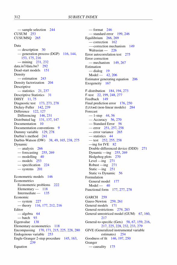
312 SUBJECT INDEX
— sample selection 244CUSUM 253CUSUMSQ 265
Data— description 30— generation process (DGP) 116, 144,
153, 175, 216— mining 231, 232
data.in7/data.bn7 292Dead-start models 151Density
— estimation 243Density factorization 204Descriptive
— statistics 21, 237Descriptive Statistics 31DHSY 11, 75Diagnostic test 173, 273, 278Dickey-Fuller 142, 239Difference 122, 127
Differencing 146, 231Distributed lag 131, 137, 147Documentation 10Documentation conventions 9Dummy variable 129, 278Durbin’s method 241Durbin-Watson (DW) 38, 49, 165, 238, 275Dynamic
— analysis 266— forecasting 255, 269— modelling 40— models 253— specification 224— systems 201
Econometric models 146Econometrics
Econometric problems 222Elementary — 118Intermediate — 135
Economic— system 227— theory 116, 177, 212, 216
Editor— algebra 64— batch 93
Eigenvalue 138Elementary econometrics 118Encompassing 170, 171, 215, 225, 228, 280Endogenous variable 253Engle-Granger 2-step procedure 145, 163,
239Equation
— format 246— standard error 199, 246
Equilibrium 266, 269— correction 162—-correction mechanism 149Walrasian — 226
Error autocorrelation test 275Error correction
— mechanism 149, 267Estimation
— dialog 19Model — 42, 206
Estimator generating equation 206Exogeneity 167
F-distribution 184, 194, 273F-test 22, 199, 248, 277Feedback 149Final prediction error 176, 250fitted (non-linear models) 284Forecast
— 1-step 44, 56— Accuracy 56, 270— Standard Error 56— error 251, 257, 258— error variance 265— statistics 44— test 252, 255, 258—ing for IVE 82Double-differenced device (DDD) 271Dynamic —ing 255, 269Hedgehog plots 270Level —ing 271Robust —ing 271Static —ing 251Static vs Dynamic 56
FormulationGeneral model 177Model — 40
Functional form 177, 277, 278
GARCH 259Gauss-Newton 259, 261General models 171General restrictions 279, 283General unrestriced model (GUM) 67, 160,
217General-to-specific (Gets) 58, 67, 159, 216,
217, 225, 228, 232, 233, 279GIVE (Generalized instrumental variable
estimates) 254Goodness of fit 146, 197, 250Granger
— causality 175

SUBJECT INDEX 313
— non-causality 214Graphic analysis 260, 263
Actual and fitted values 263Forecast Chow tests 264Forecasts and outcomes 263Residual autocorrelations (ACF) 263Residual density 264Residual density and histogram 263Residual histogram 264Residual QQ plot 264Residuals (scaled) 263Residuals (unscaled) 264
Grid search 84, 257Growth-rate models 146
Hannan–Quinn criterion 176, 250Hessian matrix 186
— reset 262Heteroscedasticity 155, 250
— and autocorrelation consistent standarderrors 156, 250
— test 277—-consistent standard errors 155, 250
Histogram 243, 263, 264Hypothesis
Null — 208
I(0) 37, 139, 145, 231, 238I(1) 37, 139, 145, 230, 231, 238I(2) 238Identification 203Identifying restrictions 226–228Inference 173Information
— criteria 63, 176, 250— matrix 206— set 210— taxonomy 210
Measurement — 212Relative future 211Relative past 210Relative present 211Rival models 213Theory — 212Theory of reduction 214
Contemporaneous — 151, 173Initial values 256, 262
— for RALS 256Innovation 166, 200, 204, 214Instability test 78, 278Instrument 82, 172, 253, 254Instrumental variables 167, 172, 255
— estimation (IVE) 79, 172, 253Interdependence 126
Intermediate econometrics 135Invariance 168, 169, 215
Jacobian matrix 207, 279
Kernel 243Normal — 243
Kurtosis 28, 33, 276, 277
Lag— length 268— operator 136— polynomial 136— weights 268Mean — 148–150Median — 148, 150Roots of — polynomials 138
Lagged— dependent variable 175, 275
Leading indicators 146Likelihood 185Line search 256, 261Linear
— combinations 180— dynamic equations 136— least-squares approximation 152— restrictions test 194, 278— systems modelling 178— transformations 180, 223
LM-test 173, 209, 256Local DGP (LDGP) 216Log-likelihood 186, 249
— function 185, 206Concentrated — 249
Log-normal distribution 272Log-t-normal distribution 272Logarithm 119Logit 100, 259, 260loglik (non-linear models) 284Long run 138, 231, 267
— equilibrium 149— solution 138, 266Static — 266
LR-test 63, 173, 209, 273Lucas critique 145, 178, 211, 228
Marginal— distribution 180, 183— model 168, 191, 226
Maximum likelihood estimation 186, 187,199, 260
Mean 121Mean Absolute Percentage Error (MAPE)
56, 270

314 SUBJECT INDEX
Measurement information 212ML 98, 259, 260, 284
Potential problems 98Tips 99
Model— design 116, 175–177, 224, 232— estimation 42, 206— evaluation 207, 263— formulation 40— output 43— reduction 58— revision 66— selection 175— tests 208Constant term 18, 41Lag selection 41Seasonals 41Typology 143, 144, 232
Model Category 16Model Class 16Modelling
— criteria 176— strategies 216— strategy 228, 279
Monte Carlo 135Multicollinearity 222Multiple
— correlation 197— regression 26, 153, 183, 190
Multivariate normal distribution 182
NLS 88, 98, 164, 258, 260, 284Potential problems 98Tips 99
Non-linear— least squares 88— modelling 98
Non-linear models 284Non-nested hypotheses 225Non-parametric
— density estimation 243Non-stationarity 230, 231Nonsense
— correlations 145— regression 133, 140
Normal— distribution 179, 186, 243— kernel 243
Normality— test 28, 33, 238, 276
Numerical— accuracy 99, 223— derivative 261, 279
— differentiation 207— optimization 84, 98, 164, 258, 261, 262— problems 261
OLS 126, 153, 172, 191, 196, 245Omitted variables 195, 225, 279Options 53Order condition 203Orthogonal
— parametrization 132, 224, 230Ox Batch Code 95OxMetrics 3, 20, 93, 286
Parameter— constancy 168, 200, 227, 252, 255,
258, 278— constancy test 258— instability 278Changing — 229Constant — 228Variation-free 206, 226
Parsimonious encompassing 171, 177, 213,228, 255, 280
Parsimony 177Partial
— adjustment 147, 151— autocorrelation 129— autocorrrelation function (PACF) 263,
274— correlations 22, 126, 198, 247
Partial autocorrelation function 241Parzen window 242PcGive Dialogs
Model 16PcGive dialogs
Estimate Model 42Forecast 55Formulate 17
Previous models 18Recall 18
Formulate Model 41Formulate Non-linear Model 88Further Output 44, 54Graphic analysis 23Model Settings 42Non-linear estimation control 89Options 53Recursive graphics 78
PcGive menusModel menu
Cross-section regression 244Descriptive Statistics 36Encompassing 65Formulate 77
SUBJECT INDEX 315
Non-linear modelling 260Options 53Progress 61
Test menu 23Dynamic analysis 46, 52Exclusion Restrictions 24, 50Forecast 55Further Output 54General Restrictions 51Graphic analysis 23, 45Linear Restrictions 24, 50Omitted Variables 26, 52Recursive graphics 78Test 48Test summary 48
PcGive unit-root test 48, 158, 267PcNaive 135Periodogram 242Poisson regression 259Population 122, 126, 188Portmanteau statistic 166, 274Predictive failure 228, 229Principal components 223, 224Principal components analysis 240Probit 100, 259Progress 61, 279
QQ plot 122, 243QR decomposition 246, 254Quasi Newton 261
R2 22, 197, 248, 249— Relative to difference and seasonals
250RALS 82, 149, 165, 176, 257
— estimation 255— grid 85— model evaluation 87Autoregressive least squares 256
Random walk 145, 238with drift 238
Rank condition 203Recursive
— estimation 77, 168, 199, 245— graphics 264
Reduced form 81— estimates 81, 254Restricted — 82, 280
Reduction 232— sequence 279
Regime shifts 211, 226, 230Regression
— coefficients 20, 246— equation 151, 191, 246
— estimates 20— graphics 23— output 21Coefficient standard error 21, 125Equation standard error 22, 125Fitted values 21Residuals 21Scalar — 123Standard error 199, 246, 247Static — 145
RESET 278RESET23 278Residual
— QQ plot 264— autocorrelation 145, 147, 224— autocorrelations 263, 274— density 263, 264— distribution 264— partial autocorrelations (PACF) 263,
274— spectrum 264— sum of squares 22, 125, 153, 192, 248,
264Store — in database 29, 50, 290
Restricted reduced form 82, 280Restrictions 227, 283Revision 212Rival models 170, 213RIVE 245, 264RLS 77, 168, 245, 264RML 245, 264RNLS 245, 258, 261, 264Root Mean Squared Error (RMSE) 55, 270Roots 138
Sample— period 119, 245— selection by a variable 244— variability 131
Scatter plot 123Schwarz criterion 161, 176, 250Score 186Seasonal 122
— means 250Selection issues
Model selection 175Sequential
— factorization 215— reduction 279— simplification 61, 177
Serial correlation 134, 149sigma 247Significance 273

316 SUBJECT INDEX
Similarity 37Sims critique 145, 226Simultaneous equations
— bias 226Single-equation Dynamic Modelling 35Skewness 28, 33, 276, 277Specific-to-general 58, 156, 177, 227Spectral density 242
Bias 242Spectrum 264Spurious regression 134Squared partial correlation 247Standard deviation 32, 121, 179, 277
Using T versus T − 1 22, 33, 249Standard error
Equation — 22, 247Standardized innovations 200, 265Staring PcGive 15Starting values 245, 261Static
— forecasting 251— long run 266— regression 145, 239
Stationarity 136, 138, 139Statistical system 228Step length 261, 262Stepwise regression 233Strong exogeneity 275Structural
— change 252— estimates 81— model 202, 227
Structural breaks 234Sufficient statistics 190, 214Summary statistics 21Super exogeneity 211, 227, 228
t-distribution 184, 194, 247t-probability 246t-value 21, 36, 126, 246Teaching econometrics 118Technical progress 231Test
— types 209ARCH — 277Augmented Dickey–Fuller — 38, 79, 142,
238, 240Autocorrelation — 176, 209, 275, 278Chow — 169, 209, 253Cointegration — 142COMFAC 160, 224, 268Durbin-Watson 38, 49, 238, 275Encompassing — 280
Exclusion Restrictions 24Forecast — 252, 255, 258Functional form mis-specification 277General restrictions 279, 283Heteroscedasticity — (squares and
cross-products) 277Heteroscedasticity — (squares) 277Instability — 78, 278Linear restrictions 24, 194, 278Normality — 28, 33, 238, 276Omitted variables 26, 154, 279Parameter constancy 200, 255, 258, 278PcGive unit-root — 48, 158Portmanteau statistic 274RESET 278Significance 209Specification — (IVE) 81, 255Testing beta = 0 (IVE) 81, 255Unit-root — 36, 157, 231, 238, 267Zero forecast 253
Theory consistent 232Theory of reduction 232Time dependence 127Time series 162Tobit 105, 259Trend 122, 239Tutorial data set (DATA) 292Two-stage least squares 80Typology 143, 144
Autoregressive errors 148Dead-start models 151Distributed lags 147Error correction mechanism 149Growth-rate models 146Leading indicators 146Partial adjustment 147Static regression 145Univariate autoregressive processes 145
Unit root 79, 141, 150— test 36, 157, 238, 267
Univariate autoregressive process 145Unrestricted reduced form 228, 255, 280
Variable— names in batch 290Endogenous — 253Instrumental — 79, 172, 253–255
Variance matrix 251, 258Variation
— across a variable 120— over time 119
Vector autoregression (VAR) 202, 226, 228

SUBJECT INDEX 317
Wald test 209, 279Weak exogeneity 144, 150, 152, 167, 168,
202, 205, 206, 215, 226White noise 166, 204, 224Wrong sign 150, 196, 214
Yule–Walker equations 241
Zero Forecast innovation mean 253