NBER WORKING PAPER SERIES

PAY-TO-BID AUCTIONS

Brennan C. PlattJoseph Price

Henry Tappen

Working Paper 15695http://www.nber.org/papers/w15695

NATIONAL BUREAU OF ECONOMIC RESEARCH1050 Massachusetts Avenue

Cambridge, MA 02138January 2010

The authors are grateful for the thoughtful comments of Lars Lefgren, Tim Salmon, Chris Cotton,and Andrzej Skrzypacz. This research was supported by a Mentoring Environment Grant at BrighamYoung University. The views expressed herein are those of the authors and do not necessarily reflectthe views of the National Bureau of Economic Research.

NBER working papers are circulated for discussion and comment purposes. They have not been peer-reviewed or been subject to the review by the NBER Board of Directors that accompanies officialNBER publications.

© 2010 by Brennan C. Platt, Joseph Price, and Henry Tappen. All rights reserved. Short sections oftext, not to exceed two paragraphs, may be quoted without explicit permission provided that full credit,including © notice, is given to the source.

Pay-to-Bid AuctionsBrennan C. Platt, Joseph Price, and Henry TappenNBER Working Paper No. 15695January 2010JEL No. D44,D53

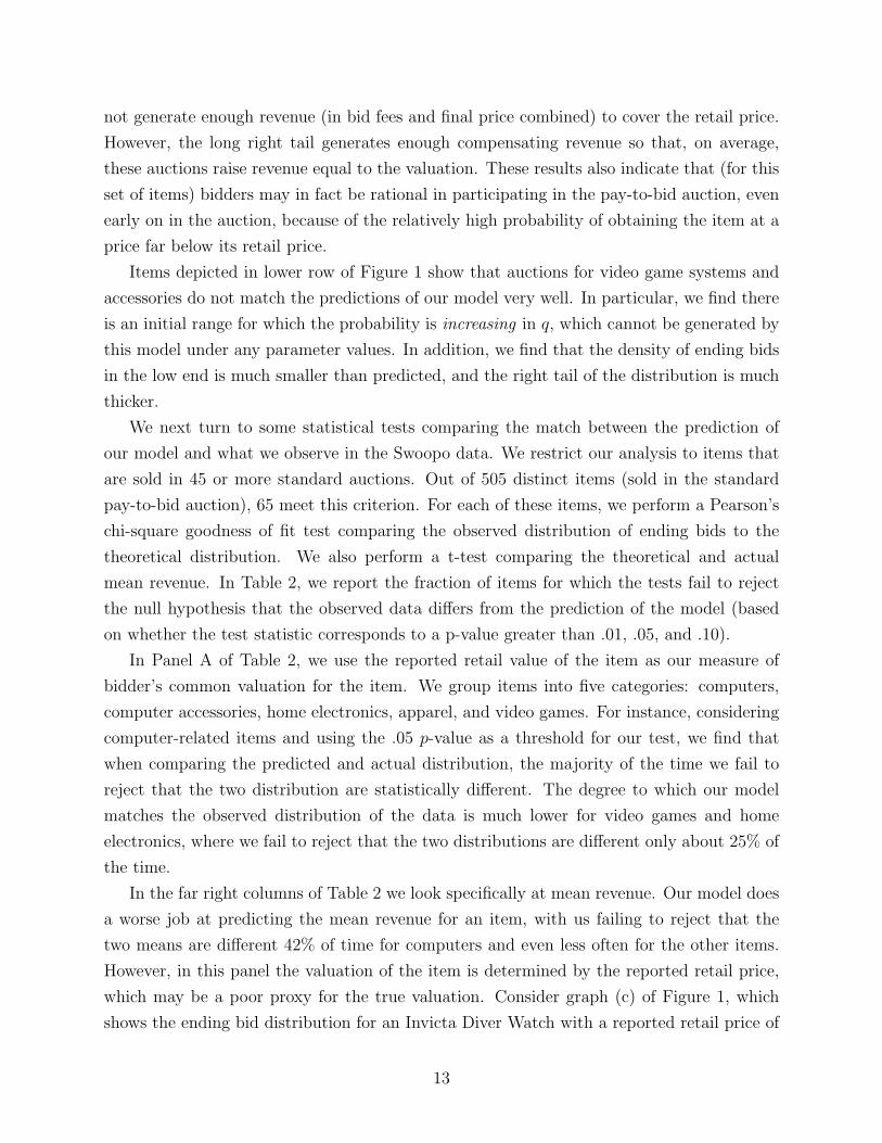
ABSTRACT

We analyze a new auction format in which bidders pay a fee each time they increase the auction price.Bidding fees are the primary source of revenue for the seller, but produce the same expected revenue asstandard auctions. Our model predicts a particular distribution of ending prices, which we test againstobserved auction data. Our model fits the data well for over three-fourths of routinely auctioned items.The notable exceptions are video game paraphernalia, which show more aggressive bidding and higherexpected revenue. By incorporating mild risk-loving preferences in the model, we explain nearly allof the auctions.

Brennan C. PlattBrigham Young Universitybrennan_platt@byu.edu

Joseph PriceDepartment of EconomicsBrigham Young University162 FOBProvo, UT 84602and NBERjoseph_price@byu.edu

Henry TappenBrigham Young University130 FOBProvo, UT 84602htappen@gmail.com

Pay-to-Bid Auctions

Brennan C. Platt, Joseph Price, and Henry Tappen∗†

January 15, 2010

Abstract

We analyze a new auction format in which bidders pay a fee each time they in-

crease the auction price. Bidding fees are the primary source of revenue for the seller,

but produce the same expected revenue as standard auctions. Our model predicts a

particular distribution of ending prices, which we test against observed auction data.

Our model fits the data well for over three-fourths of routinely auctioned items. The

notable exceptions are video game paraphernalia, which show more aggressive bidding

and higher expected revenue. By incorporating mild risk-loving preferences in the

model, we explain nearly all of the auctions.

1 Introduction

The relatively minor setup cost of internet websites has facilitated the creation of many

varieties of auction formats. Most of these have close analogs to auctions that have existed

for centuries prior, but occasionally a site develops a novel approach. Such is the case

with Swoopo, a German company founded in 2005 which currently operates websites in the

United Kingdom, Spain, the United States, and Austria. Swoopo’s distinctive feature is that

participants must pay a fee each time they place a bid.

Each auction begins at a price of zero and with a specified amount of time on a countdown

clock. When a participant places a bid, the current price increments by a fixed amount ($0.15

in the standard auction), the bidder is immediately charged a bid fee ($0.75), and the auction

∗Department of Economics, Brigham Young University, 149 FOB, Provo, UT 84602, (801) 422-8904,brennan platt@byu.edu.†The authors are grateful for the thoughtful comments of Lars Lefgren, Tim Salmon, Chris Cotton, and

Andrzej Skrzypacz.

1

is extended by a set amount of time (15 seconds).1 If the time expires before another bid is

placed, the last bidder pays the current price (on top of any bid fees incurred) and wins the

object.

An observer’s first experience with this auction format typically follows a predictable

course. First, the newcomer notes that the current price on her particular item is remarkably

low — indeed, the median auction closes with a final price that is 18.9% of the retail price.

The clock is within seconds of expiring, yet our observer quickly realizes that the deal is

elusive, as additional bids are placed every five to ten seconds. Indeed, her past bids (had

she placed any) are sunk, having no bearing on her likelihood of winning once she is outbid.2

Ideally, she would wait and place the last bid, but she immediately recognizes this to be

the fundamental dilemma of the auction: though it is highly likely that new bids will be

submitted right now, there is a small chance that none will and the auction will end.

On appreciating the low probability of winning, thoughts turn to how much revenue the

auction generates: for every dollar increase in the final price, Swoopo collects five dollars in

additional revenue through bid fees. To make a profit, the final price only needs to exceed

one-sixth of the item’s cost. This thought process has led many to question the rationality of

auction participants as well as the ethics of the auctioneers. Blogs and news articles (Kato,

2009; Reklaitis, 2009; Gimein, 2009) have vented their frustrations, referring to Swoopo as

gambling or an outright scam.

Even so, pay-to-bid auctions are growing in popularity. In December 2008, 11 websites

conducted such auctions; by November 2009, the format had proliferated to 35 websites.

Over the same time span, traffic among these sites (reported in Table 1) has increased from

1.2 million to 3.0 million unique visitors per month.3 For comparison, traffic at ebay.com

fluctuated around 75 million unique visitors per month throughout that period. In other

words, pay-to-bid auctions have garnered 4% of the traffic held by the undisputed leader in

online auctions.

We provide a simple model of the pay-to-bid auction format that rationalizes the behavior

of bidders. The key insight of this model is that the aggregate probability of being outbid

is pinned down by the requirement that prior bidders had to be willing to bid ex-ante. As

1In an English auction, this last feature is known as a soft close. Extending the clock ensures thatparticipants always have an opportunity to respond after being outbid, often expressed in oral auctions as“Going once, going twice, sold!” Amazon.com used to offer English auctions with a soft close, while e-Bayuses a hard close where the ending time is fixed (See Roth and Ockenfels, 2002).

281.3% of the unique usernames participate but never win an auction.3Web traffic was monitored using the web analytics of compete.com. The pay-to-bid industry does not

seem to be consolidating, either. Over this time period, almost all of the 35 sites experienced growth intraffic. Moreover, the concentration of traffic has fallen: in December 2008, the top two sites (includingSwoopo) claimed 90% of the market. By November 2009, the top five sites (including Swoopo) jointly held75% of the market. Bid fees have fallen, though; many (including Swoopo) are now charging $0.60 per bid.

2

a consequence, we can derive a density function describing the probability that the auction

ends at any given number of bids. From this, we show that the pay-to-bid auction raises

an expected revenue that is nearly equal to the bidders’ valuation of the item (and thus

equivalent to the revenue that standard auction formats would achieve in this environment).

We test the predictions of our model using information on 34,000 auctions collected from

Swoopo’s website.4 We find that the average revenue of most items falls within one standard

deviation of the expected revenue predicted by our model. Moreover, for most items, the

observed distribution of ending prices fits remarkably well to the distribution predicted by

the model; we fail to reject (at p = 0.05) that the distributions differ for 79% of the routinely

auctioned items.

The one group of items which do not fit our basic model are those that involve video game

systems (such as the Wii, Playstation, or Xbox), which produce more aggressive bidding and

higher revenue for Swoopo. However, the model can mimic this behavior by changing bidders’

utility from risk-neutral to risk-preferring. With very reasonable levels of absolute risk

preference (less than half of that estimated for racetrack bettors), the theoretical expected

revenue and ending price distribution line up with the observed data for 97% of the auctioned

items.

We assume that the valuation of the item is known and the same across all potential

bidders. Although first- or second-price auctions are seldom modeled in a full-information

environment, this assumption is quite common in all-pay or war-of-attrition auctions,5 which

are the closest relatives of the pay-to-bid auction. The common value allows us to isolate a

key aspect of pay-to-bid auctions: a bidder is gambling that others who value the item at

more than the current price may still abstain from bidding. We believe that this would still

be the driving force (though less visibly) in a private valuation framework.

Furthermore, a common value is quite plausible for the types of items regularly auctioned

on Swoopo. All items are new, unopened, and readily available from traditional or internet

retailers. Unlike rare art or collectibles, the market prices of these items are well established.

Indeed, one could interpret the valuation in our model as the lowest price for which the item

may readily be obtained elsewhere (rather than as the individual’s literal reservation price).

With that interpretation, the payoff from placing a bid is always relative to the utility of

buying the item outright.

Finally, it should be noted that our common value model matches the data very well.

For instance, one might speculate that the auction of a wristwatch that sells at retail for

4Our empirical approach most closely resembles that of Lambson and Thurston (2006).5Examples include Baye, et al (1996), Clark and Riis (1998), Barut and Kovenock (1998), and Konrad

and Leininger (2007). Alcalde and Dahm (2009) analyze the first-price auction in a complete informationenvironment.

3

$300 is largely driven by people who only value the watch at $50 and are hoping to win

early in the auction. However, one must consider the probability of being outbid; since an

identical watch is auctioned many times, we can extract that probability. The data speaks

very clearly on this: whether early or late in the auction, if a person values the watch at less

than $300, his expected payoff from bidding will be less than the $0.75 bid fee.

At first glance, one might consider the pay-to-bid auction as a mere reformulation of the

all-pay auction. There, each participant pays what he bids, even though only the highest

bidder wins the item. A second-price all-pay auction (or war of attrition) does the same

except that the winner pays the second highest bid. These are typically modeled in a static,

sealed-bid environment6, but their strategic properties differ significantly from the pay-to-bid

auction even when set up in the same dynamic format.

The analogy arises because each time an all-pay participant raises his bid, he commits

to pay that increase regardless of whether he wins, and is hence like a bid fee. However, in a

pay-to-bid auction, the bid fee is distinct from the price increment, and the winning bidder

must pay the final price on top of his bid fees. Moreover, in an all-pay auction, if any active

bidder increased the bid, every active bidder would have to likewise increase their own bids

to remain active (much like calling a bet in poker). A pay-to-bid participant only incurs a

bid fee each time he increases the price.

Pay-to-bid auctions share more in common with work on bidding costs, defined as trans-

action costs that the bidder incurs but are not received as revenue for the seller. These might

include legal or consultant expenses in preparing a bid or an increasing cost of financing due

to capital market imperfections.7 In one key aspect, bid costs and bid fees are similar: a

participant only places a bid if his expected payoff is sufficient to cover the certain cost.

Since valuation is homogenous in our model, this imposes our indifference condition. In

the bidding cost models, the cost discourages those with low valuations from participating.

Indeed, when bidding costs are modeled in an ascending auction (e.g. Daniel and Hirshleifer,

1998), participants conserve on bid costs by making jumps in the bid rather than raising the

current price by the minimum increment. In our setting, the bid increment is fixed.8

6See Amann and Leininger (1996), Baye, et al (1996), and Krishna and Morgan (1997). An exception isin Horner and Sahuguet (2007), where two rounds of bidding are allowed.

7Che and Gale (1998) assume that only the winner of the auction incurred the bid cost, while Gavious,Moldovanu, and Sela (2002) allow all bidders to incur the bid cost; both are set in a static, sealed-bidenvironment.

8Allowing jump bids in ascending auctions introduces a variety of strategic behaviors. One may use ajump bid to signal his private value (Daniel and Hirshleifer, 1998), to intimidate an opponent and thus inducean asymmetric equilibrium (Avery, 1998), or, for impatient participants, to finish the auction faster (Isaac,et al , 2007). We are confident that similar issues would arise in pay-to-bid auctions if jump bidding wereallowed, though it would diminish the importance of bid fees as a source of revenue and seriously complicatethe analysis.

4

The paper proceeds as follows: in section 2, we present the model and identify its unique

symmetric equilibrium. We also discuss several variations on the model. In section 3, we

discuss the data we have extracted from Swoopo’s website. Section 4 presents evidence on

the model’s fit to the data and section 5 offers conclusions and some broader applications of

the pay-to-bid auction.

2 Model

An item being sold has a known, objective value of v to all potential bidders. This is initially

offered at a price of 0. A customer immediately pays b dollars each time she places a bid,

which also increments the price by s dollars and starts a new period. The auction concludes

if no one places a bid during the current period, resulting in the last bidder paying the

current price and receiving the item. Assume that potential bidders’ decisions of when (if

at all) to act are distributed without atoms throughout each period; thus ties never occur.

This constitutes a full information, extensive form game; we examine the symmetric subgame

perfect equilibria.

When a customer places a bid, she is betting b dollars that no one else will bid after her.

Consider a customer who observes the current price at s · (q−1) dollars. If she were to place

the qth bid, her expected payoff would be (v − s · q)(1 − µq+1) − b, where µq+1 denotes the

probability that anyone else will place the q + 1th bid. She weighs the expected payoff of

winning against the certain cost of the bid fee.9

Let Q ≡ v−bs

, and for simplicity, assume that Q is an integer. If q > Q, then this customer

will strictly prefer not to bid — regardless of µq+1 — because the current price plus bid fee

exceeds the item’s value. Thus, µq = 0 for all q > Q. If q = Q, this customer is indifferent

about bidding (even though µQ+1 = 0 and hence winning is assured). Indeed, during this

and all earlier periods of the game, the participants must be indifferent about bidding. If

the qth bidder strictly preferred bidding, then µq = 1 and therefore the q− 1th bidder would

strictly prefer not to bid. If the qth bidder strictly preferred not bidding, then µq = 0 and

therefore the q − 1th bidder would strictly prefer to bid.

This indifference condition then determines unique probabilities that define equilibrium

behavior. In particular, for all 1 < q ≤ Q, µq = 1 − bv−s·(q−1)

. Only the likelihood that

anyone places the first bid, µ1, is non-unique, since there is no prior bidder who must be

made indifferent. While any µ1 ∈ [0, 1] is consistent with equilibrium, we set µ1 = 1 − bv

9One might wonder if the expected payoff should also include an option value of placing a bid; that is,a bidder might place the qth bid even if he will be outbid for certain, because it keeps the auction runningand gives him a chance to place the q+ 2th bid. However, in equilibrium, the expected payoff of placing theq + 2th bid (net of the bid fee) is zero, so a bidder at period q can ignore the option value.

5

for simplicity, assuming in effect that the first period behavior mimics that of subsequent

periods. This assumption has minimal impact on our analysis, only slightly altering expected

revenue.

We also recognize that other asymmetric equilibria can exist. For instance, suppose the

100th bidder threatens that she will place the 102nd bid with probability 1 if anyone outbids

her. This would dissuade all other participants from placing what would be a wasted 101st

bid. While such equilibria can exist, our analysis ignores them for two reasons. First, the

equilibrium would be difficult to implement if bidders are anonymous, since all potential

bidders would need to know the bidder’s specific threat.10 Second, if it were possible to

credibly communicate such threats, the obvious solution is to employ them after the first bid.

Our empirical observation does not reflect this sort of behavior, but matches the symmetric

mixed strategy equilibrium very well.

2.1 Individual strategies

The probabilities µ represent the aggregate consequence of individual mixed strategies. By

specifying the process by which bidders participate in the auction, we can analyze these

individual decisions and interpret the aggregate probabilities better. However, the aggregate

is sufficient to analyze the outcome of the auction.

First, consider an environment in which a fixed pool of n participants are watching the

auction. In the qth period, every individual chooses a mixed strategy βq on the probability of

placing a bid, taking the others’ choices as given. In a symmetric equilibrium, this will bear

direct relation to the aggregate probabilities. Suppose that q−1 bids have been placed. The

n − 1 customers who currently are not winning must decide whether to place a bid. With

probability (1 − βq)n−1, none of them do. In order to satisfy the indifference condition for

the q − 1th bid, this must equal 1− µq. So βq = 1− (1− µq)1

n−1 .

Suppose instead that bidders arrive to the auction according to a Poisson process, with

rate λ per minute. Upon arrival, the bidder instantaneously decides whether to bid (em-

ploying mixed strategy βq). If he declines to bid or someone bids after him, he departs the

auction. Again, consider after the q − 1th bid has just been placed. If a period lasts T

minutes, the probability that n customers arrive is e−λT (λT )n

n!, and the probability that all of

them decline to bid would be:

10Andrzej Skrzypacz suggested creating a username “will outbid you over five bucks” to announce yourstrategy. Perhaps to prevent such communication, Swoopo limits the length and content of usernames.Moreover, only the last ten bidders are shown, making it difficult to establish a reputation during theauction.

6

∞∑n=0

e−λT (λT )n

n!· (1− βq)n = e−λTβq

In order to satisfy the indifference condition for the q − 1th bid, this must equal 1 − µq;

however, it may not be able to do so. In particular, if λ and q are sufficiently small, we could

have e−λTβq > 1 − µq for any βq. Even so, equilibrium still exists, with minor adaptation.

Individual mixed strategies would be βq = min{− ln(1−µq)

λT, 1}

, with aggregate probability

that someone bids set to 1 − e−λT when the latter case holds. In such an equilibrium, all

bidders who arrive when q is low will strictly prefer to bid even knowing that those who

follow will do the same, because there is a large enough chance that no one will show up at

all. For high enough q, eventually the indifference condition will hold and µq again describes

the aggregate probability.

2.2 Expected revenue

In examining the expected revenue of a pay-to-bid auction, we first consider one particular

variant in which customers bid for the right to purchase an item at a predetermined price

p. In practice, Swoopo still increments the price after each bid as if s = 0.15 (which allows

us to determine the number of bids which occurred), but ignores sq in computing the final

price. The special case when p = 0 is referred to as a 100% off auction, where nothing is

paid beyond the bid fees.

The advantage of examining these fixed price auctions is that it produces a simple prob-

ability distribution. Since indifference requires that (v − p)(1 − µq) − b = 0, we derive

µq = 1− bv−p for all q. This conditional probability (that the qth bid occurs, given that the

q − 1th already has) allows us to construct the probability density that the auction ends at

exactly q bids:

f(q) =b

v − p

(1− b

v − p

)q. (1)

We then examine the expected revenue:

∞∑q=1

(bq + p)f(q) = v − vb

v − p(2)

and variance of revenue:(v − vb

v−p

)2

f(0) +∑∞

q=1

(bq + p− v + vb

v−p

)2

f(q) =(v−p−b)((2v−p)bp+(v−p)3)

(v−p)2 (3)

We note that this auction is not any more lucrative than standard auction formats. A typical

7

1st or 2nd price sealed-bid auction among (nearly) identical buyers would raise a revenue

close to v. Yet here, in the instance of a 100% off auction, the expected revenue is essentially

the same, at v − b.In the standard pay-to-bid auction, µq varies with q, which significantly complicates the

probability density function of ending bids, f(q). In particular, we obtain

f(q) ≡ (1− µq+1)

q∏j=1

µj =b

v − s · q

q∏j=1

(1− b

v − s · (j − 1)

), (4)

with f(0) = 1 − µ1. This density function is decreasing in q; that is, the unconditional

probability of ending at a given number of bids decreases as bids increase. The expected

revenue is more difficult to directly derive with this density function, but this is done in the

appendix, again arriving at an expected revenue of v − b and variance of b(v−b)(s+v)b+2s

.

The former can also be shown via an indirect method. Assuming that the seller places

no intrinsic value on the item, the total expected surplus of the auction is equal to v times

the probability that someone wins the auction, or in other words, the probability that at

least one bid is placed. This computation yields v · µ1 = v ·(1− b

v

)= v − b. This expected

surplus is split between the seller and buyers, yet by construction, the expected surplus of

the buyers is zero; hence, the seller’s expected revenue is v − b.As we noted before, µ1 is not uniquely determined by an indifference condition, though

the preceding analysis selects µ1 to be congruent with the other µq. The only impact of this

choice is seen in expected revenue: if for instance the first bid always occurred, expected

revenue would be v. While such equilibria do exist, we find it less plausible that the first bid

would be dramatically different from those that follow. Moreover, in our empirical findings

which follow, we do in fact observe a small proportion of auctions concluding without a single

bid, consistent with our selected equilibrium.

2.3 Shill bidding

One concern about this auction format is that it could be manipulated by the auctioneer

to generate more revenues; indeed, a popular accusation against Swoopo is that the website

employs shill bidders (who place bids for free to drive up the final price). As shown in the

remainder of the paper, our model is able to explain the observed data without incorporating

any malfeasance from the auctioneer, but we can offer two comments on shill bidding.

One must ask what the equilibrium response would be if shills were employed. For

instance, if shills always ensure that bidding on an item continues through at least 100 bids,

then real participants would (in equilibrium) have no reason to waste a bid in that initial

8

range, since they will certainly be outbid. This is equivalent to starting the auction with an

initial price of 100s. This increases the expected final price, but reduces the revenue from

bid fees by 100b. The net effect produces the same expected revenue of v − b.More likely, a shill would operate by randomly bidding, allowing some auctions to close

with very few bids. If so, in equilibrium, the added probability of bidding by shills displaces

some of the probability of bidding by real participants — yet the aggregate probability of

a bid occuring, µq, must maintain the indifference condition to keep the real participants

participating. For simplicity, suppose that a shill places the qth bid with probability 0 <

σq < µq. After a shill places a bid, she will win the auction with probability 1−µq+1; if that

occurs, the auctioneer retains the item but receives no revenue from the final price, though

he does collect the bid fees of all real participants.

This shill arrangement is reflected in the following expression of expected profits (i.e.

expected revenue minus the probability of a real bidder winning times v):

E[π] =

Q∑q=1

(1− σq)(sq − v)(1− µq+1)

q∏j=1

µj +

Q∑q=1

b(1− σq)q∏j=1

µj.

The first summation determines expected profit from the auction winner, who is a real bidder

with probability 1−σq and pays sq in the final price, but requires delivery of the item, causing

the auctioneer to incur cost v. Neither occurs if a shill bidder wins. The remaining terms

of the first summation represent the aggregate probability of ending at q bids. The second

summation computes expected revenue from bid fees. The product indicates the aggregate

probability that qth bid occurs, which is multiplied by b(1−σq), the expected bid fee revenue

from that bid since shill bidders do not actually pay.

After substituting for µq+1, this simplifies to

E[π] = −Q∑q=1

(1− σq)bq∏j=1

µj +

Q∑q=1

b(1− σq)q∏j=1

µj = 0.

To compare this to our previous expected revenue, note that without shill bidding, the

expected cost to the seller is v · µ1 = v − b, which also give an expected profit of 0. Shill

bidding of this form produces no additional profit.

3 Data

From the inception of their US website in September 2008 through January 2009, Swoopo.com

auctioned over 34 thousand items, all via pay-to-bid auctions. Most of these auctions are

9

repetitions of identical objects, with only 623 unique items. Furthermore, a small handful

of items are auctioned much more frequently than the others; only 65 items were auctioned

more than 45 times, with the most popular (a Nintendo Wii system) being auctioned 2,728

times. In Table 2, we group these frequently-auctioned items into 6 categories (video games,

computer accessories, apparel, etc.) and report the number of unique items and total number

of auctions for each category.

Swoopo lists all of their ended auctions on their website. For each auction, the site

provides the suggested retail price, the final auction price, the bid fees paid by the winner,

and the end time. Also listed is the bid fee and the price increment that occurs with each

new bid. Most auctions increase by $0.15, but penny auctions increase by $0.01. We divide

the final price by the bid increment to get the total number of bids in each auction. We

multiply the number of bids by the bid fee and add this to the final price to determine

Swoopo’s total revenue for that auction.

While all Swoopo auctions involve the same bid fee, there is some variety in the rules

for final prices. During this observation period, two-thirds of all Swoopo auctions followed a

standard pay-to-bid auction in which the winner pays the final auction price. The others used

the fixed price variation, where the winner pays a predetermined price. The most common

of these (12% of all auctions) was a 100% off auction, where the winner of the auction pays

nothing for the item except for the money already paid in bid fees.11

In many cases the suggested retail price is significantly higher than what is readily avail-

able from other online retailers. To provide an alternative measure of retail price, we found

each item on Amazon.com. By this measure, Swoopo’s suggested retail price is about 28%

higher than the price on Amazon.com (weighting items by the number of auctions for that

item).

Swoopo also provides the usernames of the winner and last 10 bidders of each auction.12

Across all of the auctions in our sample, there were 15,540,820 bids placed, of which 2%

occur as one of the last ten bids that we can observe. Among the last ten bidders across all

auctions, there are 69,519 unique usernames with 13,001 of these users winning at least one

item. Over 63% of the winners only win once and a very small number (less than 1%) have

won more than 25 auctions.

A common thought upon observing a pay-to-bid auction is why anyone would be the

first bidder. While it is unlikely that the first bidder will win the auction, we do have 134

auctions in which the first bidder wins the auction, 299 where the 2nd bidder does, and 8,667

11Since January 10, 2009, Swoopo has stopped offering any fixed price auctions. This may have been inresponse to criticism that 100% off auctions bore too much resemblance to a lottery or raffle.

12We cannot observe the full history of bids — that is, the identity of each bidder for each period. Thisdata would be needed to discern between the models of individual strategies developed in Section 2.1.

10

that are won by one of the first 9 bidders. In fact, two of the surprising predictions of the

model are that a large fraction of the auctions will end during the early bids and that the

(unconditional) probability of an auction ending at a given number of bids is decreasing in

the number of previous bids.

Swoopo provides bidders the option to use a bid butler which will place bids for them

based on preset parameters. To use the bid butler, the bidder decides at what price to start

bidding on an item, at what price to stop bidding on an item, and how many bids they are

willing to make. The bid butlers are designed to be as frugal as possible and will wait to bid

until there are fewer than 10 seconds left on the auction clock. We find that 32% of the last

ten bids are made using a bid butler but 64% of auctions are won by someone using a bid

butler.

Swoopo is not the only website in the US to offer pay-to-bid auctions; ten others offered a

similar service during the time period of our analysis. However, using data from a web traffic

monitoring company (Compete.com), summarized in Table 1, we found that Swoopo.com

accounted for almost half of the web traffic going to this group of sites. One of the primary

advantages of studying Swoopo is that, unlike most competitors, it provides information on

all past auctions.

4 Evidence

Our empirical objective is to test whether our model of pay-to-bid auctions appropriately

describes observed bidding on Swoopo. We test this hypothesis by comparing the observed

distribution of the number of bids to the theoretical predictions produced by our model.

While our data offers a little variation in bid fees and price increments, the overwhelming

majority charged $0.75 and raised the price by $0.15; hence, no item was auctioned enough

times outside of this standard setup to provide useful statistical inference. Even so, v has a

much greater influence on the theoretical distribution than b or s. Note that s has no impact

on expected revenue, v − b, and that b is typically two orders of magnitude smaller than v.

Where the same item has been auctioned many times, we assume that v is held constant

and that all variation in ending price is due to the equilibrium use of mixed strategies. We

repeat this analysis with 70 distinct items.

We start by providing some illustrative examples in Figure 1, showing the degree to which

the distribution of bidding behavior we observe in the Swoopo data matches the equilibrium

predictions of our model. In each example, the numbers along the x-axis are the number of

bids that occurred in an individual auction (which maps one-on-one with the revenue from

the auction). The y-axis is the probability (either theoretical or actual) that the auction

11

ends at that number of bids.

The model predicts a distribution of ending bids based on the valuation of the item, the

bid fee, and the increment by which the final price rises with each bid. The latter two are

clearly specified for each auction. For the valuation, we initially use the retail price reported

by Swoopo; however, it is quite possible that bidders may value an item more or less than

its retail price indicates. For instance, if the same item is available from internet retailers

at a discount, bidders would behave as if their true valuation is the discount price. One

would expect Swoopo bidders to be sufficiently internet-saavy to have checked Amazon.com

or similar sites for a price comparison. On the other hand, if the item were difficult to find

through other outlets, such as the Wii video game console, the true valuation could be above

retail.

To account for this possibility, we compute a maximum likelihood estimate of the param-

eter v for each regularly auctioned item, chosen to maximize∑

i ln f(qi; v), where i represents

each observed auction of that item, qi is the ending number of bids in that auction, and f is

the theoretical distribution given in Equation 4. We then repeat our statistical tests using

this estimated valuation. Figure 2(b) compares the prices we obtain using our MLE method

with those found for the same item on Amazon.com. Our MLE method provides estimates

that are higher than the Amazon (the regression coefficient on the fitted line is 0.427) but

also a very close fit along the regression line (the R2 of this regression is 0.818). In contrast,

a regression comparing Swoopo’s reported retail prices with Amazon prices has a smaller

slope of 0.365 and an R2 of only 0.570 (shown in Figure 2(a)).

We should note that using the MLE estimates for v does not enable us to shape f(q) at

will. Increasing v will lengthen the support of f and decrease its curvature in a very particular

way; moreover, it will not change that f ′(q) < 0 and f ′′(q) > 0. Also, in what follows, we

have set b and s to the objective values listed for each auction. When we simultaneously

estimated those parameters, for most auctions we recovered nearly the same objective values.

In those auctions where we did not, the fit was equally bad whether selecting only v or also

selecting b and s.

The top row of Figure 1 displays the results from three of the most common non-video

game items; the bottom row has three of the most common video game items. The upper

figures provide visual evidence that the actual distribution of revenues matches very closely

with that predicted by the model; and the fit is improved using the MLE valuations. A large

number of auctions end with few bids (and hence low revenue), and the probability of the

auction ending at q declines (at a decreasing rate) as q increases.

As a consequence, many of these auctions conclude in a net loss for Swoopo — for items

similar to those depicted in the top row, as many as 69% of the auctions of a given item will

12

not generate enough revenue (in bid fees and final price combined) to cover the retail price.

However, the long right tail generates enough compensating revenue so that, on average,

these auctions raise revenue equal to the valuation. These results also indicate that (for this

set of items) bidders may in fact be rational in participating in the pay-to-bid auction, even

early on in the auction, because of the relatively high probability of obtaining the item at a

price far below its retail price.

Items depicted in lower row of Figure 1 show that auctions for video game systems and

accessories do not match the predictions of our model very well. In particular, we find there

is an initial range for which the probability is increasing in q, which cannot be generated by

this model under any parameter values. In addition, we find that the density of ending bids

in the low end is much smaller than predicted, and the right tail of the distribution is much

thicker.

We next turn to some statistical tests comparing the match between the prediction of

our model and what we observe in the Swoopo data. We restrict our analysis to items that

are sold in 45 or more standard auctions. Out of 505 distinct items (sold in the standard

pay-to-bid auction), 65 meet this criterion. For each of these items, we perform a Pearson’s

chi-square goodness of fit test comparing the observed distribution of ending bids to the

theoretical distribution. We also perform a t-test comparing the theoretical and actual

mean revenue. In Table 2, we report the fraction of items for which the tests fail to reject

the null hypothesis that the observed data differs from the prediction of the model (based

on whether the test statistic corresponds to a p-value greater than .01, .05, and .10).

In Panel A of Table 2, we use the reported retail value of the item as our measure of

bidder’s common valuation for the item. We group items into five categories: computers,

computer accessories, home electronics, apparel, and video games. For instance, considering

computer-related items and using the .05 p-value as a threshold for our test, we find that

when comparing the predicted and actual distribution, the majority of the time we fail to

reject that the two distribution are statistically different. The degree to which our model

matches the observed distribution of the data is much lower for video games and home

electronics, where we fail to reject that the two distributions are different only about 25% of

the time.

In the far right columns of Table 2 we look specifically at mean revenue. Our model does

a worse job at predicting the mean revenue for an item, with us failing to reject that the

two means are different 42% of time for computers and even less often for the other items.

However, in this panel the valuation of the item is determined by the reported retail price,

which may be a poor proxy for the true valuation. Consider graph (c) of Figure 1, which

shows the ending bid distribution for an Invicta Diver Watch with a reported retail price of

13

$370. Our MLE estimate suggests that the true valuation is actually more like $256, which

is also in line with other online retailers. When we use the MLE-based valuation, the plot

of our predicted distribution matches the data much more closely.

In Panel B of Table 2, we use our MLE-based valuations and report the fraction of the

items in each category for which we fail to reject at each of the three common statistical

cut-offs. The goodness of fit of our model goes up for all categories; for example, with all

apparel auctions, we fail to reject a difference between the theory and data. On the other

hand, with video game items, we still only fail to reject that our predictions differ from the

data 46% of the time. In aggregate, auctions of 57 of the 72 items (or 79%) can be explained

by our theory (at the .05 p-value threshold).13

As a final piece of evidence, in Figure 3 we compare the observed average revenue with

the theoretical expected revenue, reporting the difference in standard deviation units. We

find that most of the non-video game items clump very close to zero, with 90% of these items

having average revenue within one standard deviation of the prediction of our model. For

the video-game items, we also see the mode occurring near zero but there is a large right tail

to this distribution, with 40% of the items having average revenue greater than one standard

deviation above the model’s prediction.

5 Risk preferences

To this point, we have assumed bidders to be risk neutral. We now make a minor adaptation

of our model by incorporating preferences towards risk. Since wealth is unobserved, we

sidestep this by assuming CARA utility: u(w) = 1−e−αwα

. From here, we follow the same

process as before, imposing indifference between placing a risky bid versus not participating,

then solving for µ:

(1− µq+1)1− e−α(w+v−sq−b)

α+ µq+1

1− e−α(w−b)

α=

1− e−αw

α, (5)

which yields:

µq =1− eα(b+s(q−1)−v)

eαb − eα(b+s(q−1)−v). (6)

13We also used a Kolmogorov-Smirnov test and found very similar results, with a slightly higher likelihoodof rejecting the null for some categories.

14

5.1 100% off auctions

As before we can construct a probability density function from these µ. In the special case

of 100% off auctions, this becomes:

f(q) =

(1− eα(v−b)

1− eαv

)q (eαv − eα(v−b)

1− eαv

)(7)

which generates an expected revenue of b(eα(b−v)−1

1−eαb

). Note that expected revenue is decreas-

ing in α; the auction generates more revenue as agents become less risk averse.

We can perform a maximum likelihood estimation on f(q) as before; however, α is not

separately identifiable from v or b. This is because the distribution has the form f(q) =

(1− µ)µq. Thus, the MLE procedure can only identify µ.

Fortunately, all of the items where Swoopo has routinely used 100% off auctions have an

obvious objective value for v. These items include cash ($1,000 or $80) and vouchers for free

Swoopo bids (either 300 or 50, worth $0.75 per bid). The bid fee b is also exogenously set,

so we can use the MLE procedure to identify α.

For these items, we find α to be slightly negative, between -0.001 and -0.01. This implies

that Swoopo participants are risk loving. The resulting theoretical distribution is depicted

in Figure 4; with the MLE risk preferences, the fit is remarkable. Using risk neutral bidders

(and the objective value of v), the theoretical distribution would predict too few bids at

every point and hence too high a probability of ending early. With the addition of risk-

loving preferences, bidders become a bit more aggressive at every point of the auction.

5.2 Standard auctions

After incorporating risk preferences in a standard pay-to-bid auction, the resulting proba-

bility density is far less tractable:

f(q) ≡ (1− µq+1)

q∏j=1

µj =1− eαb

eαb − eα(b+sq−v)

q∏j=1

(1− eα(b+s(j−1)−v)

eαb − eα(b+s(j−1)−v)

). (8)

Direct analytic solutions for expected revenue are no longer possible. Indeed, even the

indirect method used in the risk neutral case is no longer applicable, since the auction not

only creates value by transferring an item to someone who values it, but also creates risk,

whether for good (α < 0) or ill (α > 0). However, numerical computation is relatively

simple, revealing a few key features of f .

First, the support of f is the same as before, placing positive probability everywhere

15

from 0 ≤ q ≤ Q. Increases in v have essentially the same effect that they did in the risk-

neutral case: it will increase the support and flatten the distribution. When α > 0 (i.e.

risk aversion), f has a similar convex shape to the risk neutral density function, only with

greater curvature as α rises.

The distribution behaves quite differently for α < 0 (i.e. risk-loving). When α is very

close to zero, an inflection point q is introduced near zero such f ′′ < 0 below q; thus f is

no longer strictly convex. As α decreases, this inflection point takes on higher values, and

eventually, creates a hump-shaped distribution. As α becomes more negative, the q which

maximizes f increases.

To perform maximum likelihood estimation, we use numerical approximation of the den-

sity function. For each auctioned item, we estimate both the valuation and risk parameter,

which are identified by distinct first-order conditions of this generalized pay-to-bid distribu-

tion. Note that even with these two degrees of freedom, we are not capable of replicating

every unimodal distribution, but are constrained to the particular shape described above.

After MLE, the resulting risk parameter α indicates that bidders on video game items

are mildly risk-loving, primarily in the range of -0.001 to -0.006, with a few as low as -0.025.

These values are significantly lower than the estimated risk preferences of bettors at horse

race tracks: using the same functional form and assuming a bet (i.e. our bid fee) of £1,

Jullien and Salanie (2000) estimate α = −0.055.14 The resulting MLE valuations v are also

plausible for each item, generally below the retail price with the exception of items that were

in short supply during this data period. Figure 2(c) compares these to Amazon.com prices;

the associated regression has a steeper slope (0.571) than the risk-neutral MLE valuation in

Figure 2(b), and a slightly lower R2 of 0.756.

The improvement in fit is again remarkable. Figure 5 illustrates the new theoretical

distribution, demonstrated on the same three items from the lower panel of Figure 1. The

risk neutral model was unable to match the hump shape of the distribution because for any

choice of the parameter v, f(q) was decreasing in q. In the altered model, f(q) will first

rise then fall if α is sufficiently large; thus, early bidders are more likely to bid than risk

neutrality would imply.

Intuitively, this occurs because when q is low, there is greater variance in the outcome,

because the payoff if no one else bids, v−sq, is large. A risk-loving participant will be willing

to bid in spite of unfair odds as long as the gamble has a highly skewed payoff. Thus µq can

be larger than in the risk neutral model (more aggressive bidding) while still satisfying our

14Similar studies uses a functional form u(w) = awb, which has constant relative risk aversion. Ali (1977)assumes an initial wealth w = 1 and estimates b = 1.178, or an absolute risk aversion (comparable to our α)of -0.178. Kanto, et al (1992) and Golec and Tamarkin (1998) arrive at similar estimates.

16

indifference condition, and as a result, it is less likely that the auction ends with low q. As q

increases, though, the variance in outcome diminishes, and the same risk-loving participant

will require closer to fair odds in order to bid. Indeed, as the final price sq approaches v, the

resulting µq approaches the risk neutral result.

Panel C of Table 2 reports the degree of fit for all auctions after MLE allowing for

risk-loving preferences. Note that nearly all of the auctions can be explained by the model

once risk preferences are included. In particular, nearly 50% more video game items fit the

adapted model.15

5.3 Risk-loving preferences

It is not particularly surprising that Swoopo participants would have a preference for risk;

after all, this auction is essentially a form of gambling. Like a slot machine, the bidder

deposits a small fee to play, aspiring to a big payoff (of obtaining the item well below its

value). The only difference is that the probabilities of winning are endogenously determined.

The idea that a gambler would voluntarily take on risk, paying more than the expected

payout to play, is puzzling. Economists have tried to rationalize such behavior in one of

two routes: by assuming some intrinsic utility from placing the gamble or by assuming

convex preferences with respect to wealth.16 Regarding the former, it is noteworthy that

Swoopo prominently advertises itself as “entertainment shopping.” While many economists

have referred to intrinsic utility as motivation for gambling, very few have provided formal

modeling of the concept. Diecidue, Schmidt, and Wakker (2004) provide a brief but useful

survey of these works and offer their own formal model. They conclude that utility from

gambling would necessarily contradict stochastic dominance.

We employ the alternative: assuming convex preferences (that is, increasing marginal

utility of wealth within some range). Friedman and Savage (1948) provided an early formal

model of this phenomenon. Their justification for increasing marginal utility was that major

increases in wealth would promote a person into a new social and economic status, while

minor increases in wealth would maintain a person within the same class and hence exhibit

diminishing marginal utility. This view was supported by Gregory (1980) and Brunk (1981).

More recent work by Golec and Tamarkin (1998) and Garrett and Sobel (1999) proposes

that what appears as risk-loving in the Friedman-Savage utility should be more aptly named

skewness-loving. In an empirical study of horse-track betting and US lottery games, respec-

15Again, Kolmogorov-Smirnov tests provided nearly identical results.16In addition, much of behavioral economics is inspired by these and similar puzzles. These lines of work

offer alternatives to expected utility, such as prospect theory, ambiguity aversion, or bounded rationality, toname a few. We omit discussion of these theories because their application in a game theoretic setting is nota settled matter.

17

tively, both papers conclude that gamblers experience disutility from variance in payoffs (i.e.

are still risk averse), but gain utility from skewness in payoffs. Golec and Tamarkin show

that this will appear as risk-loving preferences when estimating parameters for CRRA utility.

This view of risk-loving behavior seems appropriate for our model, particularly for items

such as video games. The bidders may not be able to justify (to their spouse, their parent,

or themselves) spending $300 on a Wii at a retail store; however, the potential to win the

Wii early in the auction for only a fraction of that makes it worth the $0.75 gamble, even

at unfair odds. As the number of bids (and hence the final price) increase, the skewness in

outcome decreases and these gamblers are less tolerant of unfair odds. Indeed, as the final

price approaches the retail price, µq eventually adjusts so that bidding becomes a fair bet.

Figure 6 provides evidence of this behavior, plotting the expected payoff for bidding on a

Wii game system conditional on the current number of bids. The conditional expected payoff

is the probability that the auction will end before the next bid (conditional on the auction

reaching the current bid) times the net value derived by the winner (the valuation minus

the final price). The theoretical plot derives conditional probabilities from the indifference

condition, while the observed plot extracts this information from the data.

The plot of the expected payoff using the observed data is based on a two-step procedure.

First, we use a kernel regression to smooth the cumulative density function of the number

of bids at which the Wii auction ends, F (q). This is used to construct the expected payoff,

(v − sq) f(q)1−F (q)

, where the latter term is the probability of the auction ending, conditional

on the auction reaching that number of bids. We then smooth this expected payoff function

using a kernel regression and plot this function up to 1600 bids (the 95th percentile, or a

final price that is 70% of the valuation).17 The expected payoff from bidding is very low

at the start of the auction (around 22 cents) but rises because the probability of winning

increases faster than the net value of winning falls.

For more practical items such as computers or apparel, bidders behave as if they are risk

neutral.18 This probably reflects that they intend to purchase the item from a traditional

retailer if unsuccessful at Swoopo.

17For both kernel regressions we use a Epanechnikov kernel and a bandwidth of 75. The pattern in figure6 is the same when we use alternative bandwidths or use a local polynomial regression.

18The distinct behavior in video game auctions naturally raises the question of whether a different set ofbidders participate in video game versus other auctions, or if instead the same people participate in bothbut behave more aggressively in video game auctions. We were not able to follow every bid on every auction,but for a set of 1,084 auctions, we were able to record the usernames of most of the auction participants (asopposed to only the last ten). Unfortunately, even for those auctions, we lack sufficient observations for eachbidder to provide any meaningful insight on this question; only 2% of the bidders place more than 10 bids.

18

6 Conclusion

This paper presents a simple model of bidder choices in a pay-to-bid auction. In the symmet-

ric subgame perfect equilibrium, potential bidders are indifferent about participating, and

the exact mixed strategy is determined by this indifference condition. Using these mixed

strategies we can establish that expected revenue will be near the bidders’ valuation of the

auctioned item.

Even when restricted to risk neutral bidders, the model is able to explain a strong majority

of the observed data. However, items associated with video game systems routinely produce

more aggressive bidding and higher revenue than can be explained by this model. These

exceptions are the most profitable of Swoopo’s auctions, and are among the most frequently

run. Once we allow bidders to have preferences towards risk, the model can explain almost

all of the observed auctions. Buyers of video game systems have small preferences for risk

(which may be interpreted as a love of skewness), which makes them aggressive in the early

phase of the bidding.

On a broader level, the pay-to-bid auction describes an incremental king-of-the-hill con-

test. By incurring a sunk cost (e.g. bid fee), anyone can become the current king-of-the-hill;

yet that title only becomes permanent if all challengers give up. The contest is incremental

because each replacement of a king reduces the hill’s value to the eventual winner.

For instance, this could describe a particular form of competition among rent seekers.

Suppose several firms were seeking the same exclusive license from a bribe-accepting reg-

ulator. The regulator could require an up-front bribe each time a firm wishes to make an

overture; moreover, to displace the previous overture, the current firm promises to return a

greater portion of the future rents to the regulator. The license is awarded once no additional

overtures are attempted, and is given to the firm with the last (and hence best) overture. A

similar story could be told for competition among suitors, showering gifts or attention on a

potential mate.

Applied to these situations, our risk-neutral model would predict that the regulator cap-

tures essentially the full value of the license (in expectation). The firms would be indifferent

about participation ex-ante; yet ex-post, the winning firm will typically enjoy large rents,

with a final price well below the full value. If the firms are risk loving, the regulator can

expect to extract even more than the full value, making this a far more profitable means of

allocating the license than other auction formats. Indeed, risk-loving (or skewness-loving)

preferences might well be applicable if the residual rents would significantly alter the winner’s

social class or if, in the case of a suitor, the contest gives him a shot at a woman normally

far outside his league.

19

Appendix

Mean and Variance of Revenue

To facilitate the analysis of the first and second moments of the f distribution, we make use

of the ascending factorial or Pochhammer symbol: (a)k ≡ a(a + 1) · · · (a + k − 1) = Γ(a+k)Γ(a)

,

where Γ(·) denotes the Gamma function.

Expected revenue is:

ERev =

Q∑q=1

(b+ s)q(1− µq+1)

q∏j=1

µj =

Q∑q=1

(b+ s)q

q∏j=1

µj −Q∑q=1

(b+ s)q

q+1∏j=1

µj

=

Q−1∑q=0

(b+ s)(q + 1)

q+1∏j=1

µj −Q∑q=1

(b+ s)q

q+1∏j=1

µj

=

Q−1∑q=0

(b+ s)

q+1∏j=1

µj +

Q−1∑q=0

(b+ s)q

q+1∏j=1

µj −Q∑q=1

(b+ s)q

q+1∏j=1

µj

=

Q−1∑q=0

((b+ s)

q+1∏j=1

µj

)− (b+ s)Q

Q+1∏j=1

µj

The last term drops out entirely since µQ+1 = 0. Since µj = 1− bv−s·(j−1)

=b−vs

+j−1

− vs

+j−1, this

can be rewritten as:

ERev = (b+ s)

Q∑q=1

q∏j=1

µj = (b+ s)

Q∑q=1

(b−vs

)q(

−vs

)q

.

An identity of ascending factorials provides that(a)j(a)k

= (a+ k)j−k. Hence,

ERev =b+ s(−vs

)Q

Q∑q=1

(b−vs

)q(

−vs

)q

(−vs

)Q

=b+ s(−vs

)Q

Q∑q=1

(b− vs

)q

(−vs

+ q)Q−q

.

Another transformation of ascending factorials establishes that (a)n+1 − (x)n+1 = (a −x)∑n

k=0(a)k(x + k + 1)n−k. Applying it here, let a = b−vs

, x = − s+vs

, and n = Q, which

yields:

(b− vs

)Q+1

−(−s+ v

s

)Q+1

=b+ s

s

Q∑q=0

(b− vs

)q

(−s+ v

s+ q + 1

)Q−q

,

20

or, since (a)0 ≡ 1, this becomes:

(b− vs

)Q+1

−(−s+ v

s

)Q+1

=b+ s

s

((−vs

)Q

+

Q∑q=1

(b− vs

)q

(−vs

+ q)Q−q

).

This allows us to substitute for the summation in expected revenue to obtain:

ERev =b+ s(−vs

)Q

(s

b+ s

((b− vs

)Q+1

−(−s+ v

s

)Q+1

)−(−vs

)Q

).

Since (a)n+1 = (a+ n) · (a)n and (a− 1)n = a−1a+n−1

· (a)n, this simplifies to:

ERev =1(−vs

)Q

(s

(b− vs

)Q+1

+ (s+ v)(−vs

)Q− (b+ s)

(−vs

)Q

)

=s(b−vs

)Q+1(

−vs

)Q

+ (v − b) =s(b−vs

+Q)·(b−vs

)Q(

−vs

)Q

+ (v − b)

But since b−vs

+Q = 0, this yields ERev = v − b.Variance is is similarly derived:

V ar =

Q∑q=0

((b+ s)q − v + b)2 f(q)

= (v − b)2 − 2(v − b)Q∑q=1

(b+ s)qf(q) +

Q∑q=1

(b+ s)2q2f(q)

= −(v − b)2 + (b+ s)2

Q∑q=1

q2(1− µq+1)

q∏j=1

µj

With similar manipulation as above, this last sum is equal to (b−2v)(b−v)(b+s)(b+2s)

. Hence, V ar =b(v−b)(s+v)

b+2s.

21

Figure 1: Representative examples: comparison of the theoretical and actual distribution ofending bids for each item.

Notes: The unit of observation is the individual auctions for each item. In each figure, thex-axis denotes the final number of bids placed for the item. The y-axis is the probabilitythat the auction concludes at that number of bids. Bars denote the observed frequencies;the solid line gives the theoretical frequencies using the retail value and the dashed line doesthe same using the MLE estimated value.

22

Figure 2: Comparison of item valuations to Amazon.com prices

A. Retail value reported by Swoopo

B. MLE-estimated valuation

C. Risk MLE-estimated valuation

23

Table 1: Monthly traffic on pay-to-bid websites

Website # of unique visitors

Dec. 2008 Nov. 2009Swoopo.com 508,237 560,871

Ubid.com 550,802 276,649Bidcactus.com 0 788,497

Beezid.com 0 325,906Quibids.com 0 320,998

All other sites 164,792 742,431Total # of sites 11 35

All Pay-to-Bid Sites 1,223,842 3,015,352

Ebay.com 79,806,830 74,067,835Pay-to-Bid Site Traffic/Ebay Traffic 1.5 % 4.1 %

Notes: Data from compete.com, a web traffic monitoring company.

Figure 3: Deviation from Expected Revenue in risk neutral model (separately for videogames and other items)

Notes: The unit of observation is each unique item. The x-axis indicates by how many stan-dard deviations the observed average revenue differs from the theoretical expected revenue.The y-axis indicates the fraction of items auctioned with that observed outcome.

24

Table 2: Statistical tests comparing theoretical distribution with observed data.

A. Using retail price as item valuation.Pearsons χ2 Test t-Test

(compares distributions) (compares means)Item Type N obs p ≥ .10 p ≥ .05 p ≥ .01 p ≥ .10 p ≥ .05 p ≥ .01

Computers 7 521 0.571 0.571 0.714 0.286 0.429 0.429Computer Accessories 24 3434 0.375 0.417 0.583 0.292 0.333 0.417

Home Electronics 7 1651 0.286 0.286 0.429 0.143 0.143 0.286Apparel 14 1045 0.286 0.357 0.357 0.071 0.071 0.143Movies 2 97 1.000 1.000 1.000 1.000 1.000 1.000

Video Games 18 9831 0.111 0.111 0.222 0.000 0.056 0.167

B. Using MLE valuation of itemPearsons χ2 Test t-Test

Item Type N obs p ≥ .10 p ≥ .05 p ≥ .01 p ≥ .10 p ≥ .05 p ≥ .01

Computers 7 521 1.000 1.000 1.000 1.000 1.000 1.000Computer Accessories 24 3434 0.708 0.833 0.875 0.833 0.833 0.917

Home Electronics 7 1651 0.714 0.714 0.857 0.857 0.857 0.857Apparel 14 1045 1.000 1.000 1.000 0.857 1.000 1.000Movies 2 97 1.000 1.000 1.000 1.000 1.000 1.000

Video Games 18 9831 0.500 0.500 0.611 0.500 0.611 0.667

C. Using MLE risk preferences and valuation of itemPearsons χ2 Test t-Test

Item Type N obs p ≥ .10 p ≥ .05 p ≥ .01 p ≥ .10 p ≥ .05 p ≥ .01

Computers 7 521 1.000 1.000 1.000 1.000 1.000 1.000Computer Accessories 24 3434 0.875 0.917 0.917 0.833 0.917 0.958

Home Electronics 7 1651 1.000 1.000 1.000 1.000 1.000 1.000Apparel 14 1045 1.000 1.000 1.000 0.769 0.769 0.923Movies 2 97 1.000 1.000 1.000 1.000 1.000 1.000

Video Games 18 9831 1.000 1.000 1.000 1.000 1.000 1.000

Notes: The number reported in each cell is the fraction of items for which the particular teststatistic has a p-value larger than the threshold indicated in each column. N refers to thenumber of unique items in each category, while obs refers to the number of observed auctionswithin that category.

25

Figure 4: 100% Off Auctions with risk-loving bidders: comparison of the theoretical andactual distribution of ending bids for each item.

Notes: Risk MLE denotes the theoretical distribution of ending bids when MLE-estimatedbidder risk preferences is used; item value is assumed to be retail value.

Figure 5: Standard auctions with risk-loving bidders: comparison of the theoretical andactual distribution of ending bids for each item.

Notes: Risk MLE denotes the theoretical distribution of ending bids when MLE-estimateditem value and bidder risk preferences are used.

26

Figure 6: Expected payoff at each point during the auction for a Wii video game unit.

Notes: The expected payoff is the probability of the auction ending at each bid conditionalon the auction arriving at that point times the value of winning the item which is thevaluation minus the final price. The expected payoff must equal the bid fee of $0.75 to beactuarially fair, which the theoretical curve reaches at 2260 bids (i.e. when the final pricenearly equals the valuation). We smoothed the observed expected payoff function using akernel regression. Bids above 1600 are excluded from the smoothing due to the sparsenessof data in that range (fewer than 5% of the observations).

27

References

Ali, Mukhtar M. (1977) “Probability and Utility Estimates for Racetrack Bettors,” Journal

of Political Economy 85, 803-15.

Alcalde, Jose, and M. Dahm. (2009) “The Complete Information First-Price Auction with

Finite Bidding Grid,” Mimeo.

Amann, Erwin, and W. Leininger. (1996) “Asymmetric All-Pay Auctions with Incomplete

Information,” Games and Economic Behavior 14, 1-18.

Avery, Christopher. (1998) “Strategic jump bidding in English auctions,” Review of Eco-

nomic Studies 65, 185-210.

Barut, Yasar, and D. Kovenock. (1998) “The symmetric multiple prize all-pay auction with

complete information,” European Journal of Political Economy 14, 627-644.

Baye, Michael, D. Kovenock, and C. de Vries. (1996) “The All-Pay Auction with Complete

Information,” Economic Theory 8, 291-305.

Brunk, Gregory. (1981) “A Test of the Friedman-Savage Gambling Model,” Quarterly Jour-

nal of Economics 96, 341-348.

Che, Yeon-Koo, and I. Gale. (1998) “Standard Auctions with Financially Constrained Bid-

ders,” Review of Economic Studies 65, 1-21.

Clark, Derek, and C. Riis. (1998) “Competition over More than One Prize,” American

Economic Review 88, 276-289.

Daniel, Kent, and D. Hirshleifer. (1998) “A Theory of Costly Sequential Bidding,” Mimeo,

University of California, Los Angeles.

Diecidue, Enrico, U. Schmidt, and P. Wakker. (2002) “The Utility of Gambling Reconsid-

ered,” Journal of Risk and Uncertainty 29, 241-259.

Friedman, Milton, and L. Savage. (1948) “The Utility Analysis of Choices Involving Risk,”

Journal of Political Economy 56, 279-304.

Gavious, Arieh, B. Moldovanu, and A. Sela. (2002) “Bid Costs and Endogenous Bid Caps,”

RAND Journal of Economics 33, 709-722.

28

Gimein, Mark. (2009) “The Crack Cocaine of Auction Sites,” The Big Money, July

7, 2009. http://www.thebigmoney.com/articles/money-trail/2009/07/07/crack-cocaine-

auction-sites.

Golec, Joseph, and M. Tamarkin. (1998) “Bettors Love Skewness, Not Risk, at the Horse

Track,” Journal of Political Economy 106, 205-225.

Garrett, Thomas, and R. Sobel. (1999) “Gamblers favor skewness, not risk: Further evidence

from United States lottery games,” Economics Letters 63, 85-90.

Gregory, Nathaniel. (1980) “Relative Wealth and Risk Taking: A Short Note on the

Friedman-Savage Utility Function,” Journal of Political Economy 88, 1226-1230.

Horner, Johannes, and N. Sahuguet. (2007) “Costly Signaling in Auctions,” Review of Eco-

nomic Studies 74, 173-206.

Isaac, R. Mark, T. Salmon, and A. Zillante. (2007) “A theory of jump bidding in ascending

auctions,” Journal of Economic Behavior and Organization 62, 144-164.

Jullien, Bruno, and B. Salanie. (2000) “Estimating Preferences under Risk: The Case of

Racetrack Bettors,” Journal of Political Economy 108, 503-530.

Kanto, Antti, G. Rosenqvist, and A. Suvas. (1992) “On Utility Function Estimation of

Racetrack Bettors,” Journal of Economic Psychology 13, 491-98.

Kato, Donna. (2009) “Penny Auction Sites Offer Chance for Big Bargins,” San Jose Mercury

News, May 22, 2009.

Konrad, Kai, and W. Leininger. (2007) “The generalized Stackelberg equilibrium of the

all-pay auction with complete information,” Review of Economic Design 11, 165-174.

Krishna, Vijay, and J. Morgan. (1997) “An Analysis of the War of Attrition and the All-Pay

Auction,” Journal of Economic Theory 72, 343-362.

Lambson, Val, and N. Thurston. (2006) “Sequential Auctions: Theory and Evidence from

the Seattle Fur Exchange,” RAND Journal of Economics 37, 70-80.

Reklaitis, Victor. (2009) “Entertainment E-Com On Web’s Retail Stage,” Investor’s Business

Daily April 7, 2009.

Roth, Alvin, E. and A. Ockenfels. (2002) “ Last-Minute Bidding and the Rules for End-

ing Second-Price Auctions: Evidence from eBay and Amazon Auctions on the Internet,”

American Economic Review 92, 1093-1103.

29