Patterns and Practices for Future Architectures

Eric Werner Scott McMillan Jonathan Chu

August 2014

TECHNICAL NOTE CMU/SEI-2014-TN-001

Emerging Technology Center

http://www.sei.cmu.edu

Copyright 2014 Carnegie Mellon University This material is based upon work funded and supported by the Department of Defense under Contract No. FA8721-05-C-0003 with Carnegie Mellon University for the operation of the Software Engineer-ing Institute, a federally funded research and development center. Any opinions, findings and conclusions or recommendations expressed in this material are those of the author(s) and do not necessarily reflect the views of the United States Department of Defense. References herein to any specific commercial product, process, or service by trade name, trade mark, manufacturer, or otherwise, does not necessarily constitute or imply its endorsement, recommendation, or favoring by Carnegie Mellon University or its Software Engineering Institute. This report was prepared for the SEI Administrative Agent AFLCMC/PZM 20 Schilling Circle, Bldg 1305, 3rd floor Hanscom AFB, MA 01731-2125 NO WARRANTY. THIS CARNEGIE MELLON UNIVERSITY AND SOFTWARE ENGINEERING INSTITUTE MATERIAL IS FURNISHED ON AN “AS-IS” BASIS. CARNEGIE MELLON UNIVERSITY MAKES NO WARRANTIES OF ANY KIND, EITHER EXPRESSED OR IMPLIED, AS TO ANY MATTER INCLUDING, BUT NOT LIMITED TO, WARRANTY OF FITNESS FOR PURPOSE OR MERCHANTABILITY, EXCLUSIVITY, OR RESULTS OBTAINED FROM USE OF THE MATERIAL. CARNEGIE MELLON UNIVERSITY DOES NOT MAKE ANY WARRANTY OF ANY KIND WITH RESPECT TO FREEDOM FROM PATENT, TRADEMARK, OR COPYRIGHT INFRINGEMENT. This material has been approved for public release and unlimited distribution except as restricted be-low. Internal use:* Permission to reproduce this material and to prepare derivative works from this material for internal use is granted, provided the copyright and “No Warranty” statements are included with all reproductions and derivative works. External use:* This material may be reproduced in its entirety, without modification, and freely dis-tributed in written or electronic form without requesting formal permission. Permission is required for any other external and/or commercial use. Requests for permission should be directed to the Software Engineering Institute at permission@sei.cmu.edu. * These restrictions do not apply to U.S. government entities. Carnegie Mellon® is registered in the U.S. Patent and Trademark Office by Carnegie Mellon Universi-ty. DM-0001042

CMU/SEI-2014-TN-001 | i

Table of Contents

Acknowledgments iv

Abstract v

1 Background and Motivation 1 1.1 Benchmarks 3 1.2 Breadth-First Search Framework 4 1.3 Approach 7

2 Implementations 8 2.1 Single CPU, List 8

2.1.1 Kernel 1 8 2.1.2 Kernel 2 10

2.2 Single CPU, Compressed Sparse Row 10 2.2.1 Kernel 1 10 2.2.2 Kernel 2 12

2.3 Single GPU, CSR 13 2.3.1 Kernel 1 13 2.3.2 Kernel 2 14

2.4 Single GPU, Out-of-Core CSR 15 2.4.1 Kernel 1 15 2.4.2 Kernel 2 17

2.5 Multi-CPU, CombBLAS 20 2.5.1 Kernel 1 20 2.5.2 Kernel 2 21

3 Results for All Implementations 24 3.1 Performance Comparison of Individual Approaches 24

3.1.1 Single CPU/GPU Performance 24 3.1.2 Parallel CPU/GPU Performance 26

3.2 Performance vs. Code Complexity 27 3.3 Summary 28

4 Conclusions and Future Work 30

Appendix Test Hardware Configuration 32

5 References 35

CMU/SEI-2014-TN-001 | ii

List of Figures

Figure 1: Intel CPU Introductions [Reprinted from Sutter 2009] 1

Figure 2: Representations of Undirected Graphs: (a) Edge List, (b) Adjacency List, and (c) Adjacency Matrix 5

Figure 3: Example of Breadth-First Search of the Graph from Figure 2, Starting at Vertex 1 6

Figure 4: Data Structures Created by Kernel 1 of Single CPU, List Implementation Using the Graph in the Example from Section 1.2 9

Figure 5: Kernel 2 of Graph500 BFS Reference Implementation: Single CPU, List 10

Figure 6: Data Structures for Sequential CSR Algorithm 12

Figure 7: BFS Traversal Algorithm: Single CPU, CSR 13

Figure 8: GPU Implementation of BFS [Adapted from Harish 2007, 2009] 14

Figure 9: Data Structures Used in Out-of-Core GPU Algorithm 16

Figure 10: BFS Algorithm for Out-of-Core GPU Implementation 18

Figure 11: Steps of BFS Traversal Using the Graph from Figure 2 19

Figure 12: Two-Dimensional (2 × 2) Decomposition of the Example Adjacency Matrix 21

Figure 13: CombBLAS Kernel 2 Algorithm 22

Figure 14: BFS Traversal Using Semi-ring Algebra 23

Figure 15: Kernel 1 Processing Time vs. Problem Scale for All Algorithms (Lower Is Better) 24

Figure 16: Kernel 2 TEPS (Traversed Edges per Second) vs. Problem Scale (Higher Is Better) 25

Figure 17: Kernel 1 Processing Times vs. Problem Scale for Multi-CPU, CombBLAS Implementation (Lower Is Better) 26

Figure 18: Kernel 2 TEPS (Traversed Edges per Second) vs. Problem Scale (Higher Is Better) 27

Figure 19: Kernel 2 TEPS vs. Normalized Level of Effort (Scaled to Single CPU, List SLOC) 28

Figure 20: Comparison of Linear Algebra (left) and the Proposed Graph Analytics (right) Library Architectures 30

Figure 21: SGI UV 100 (CPU-Only) Configuration 33

Figure 22: SGI C2108 2U Server with Two NVIDIA Tesla GPUs 34

CMU/SEI-2014-TN-001 | iii

List of Tables

Table 1: Comparison of Implementation Source Lines of Code 27

CMU/SEI-2014-TN-001 | iv

Acknowledgments

We would like to thank Dr. Matthew Gaston, director of SEI’s Emerging Technology Center, for his guidance and expert advice during the definition and execution of this work and Alex Nicoll, of SEI’s CERT® Division, for his contributions to this work in the area of algorithms for CUDA™ graphics processing units.

CMU/SEI-2014-TN-001 | v

Abstract

Graph algorithms are widely used in Department of Defense applications including intelligence analysis, autonomous systems, cyber intelligence and security, and logistics optimization. These analytics must execute at larger scales and higher rates to accommodate the growing velocity, volume, and variety of data sources. The implementations of these algorithms that achieve the highest levels of performance are complex and intimately tied to the underlying architecture. New and emerging computing architectures require new and different implementations of these well-known graph algorithms, yet it is increasingly expensive and difficult for developers to implement algorithms that fully leverage their capabilities. This project investigates approaches that will make high-performance graph analytics on new and emerging architectures more accessible to users. The project is researching the best practices, patterns, and abstractions that will enable the development of a software graph library that separates the concerns of expressing graph algo-rithms from the details of the underlying computing architectures. The approach started with a fundamental graph analytics function: the breadth-first search (BFS). This technical note com-pares different BFS algorithms for central and graphics processing units, examining the abstrac-tions used and comparing the complexity of the implementations against the performance achieved.

CMU/SEI-2014-TN-001 | 1

1 Background and Motivation

The observation stated in Moore’s law, that the number of transistors that can be placed onto an integrated circuit doubles approximately every two years [Moore 1965], still holds true. For the bulk of the modern era, the additional transistors and increase in power efficiency resulted in con-comitant clock-speed and single-core performance increases. Within the last 10 years, however, clock-speed improvements to processors have leveled off despite transistor counts continuing to rise, as shown in Figure 1. The result is that recent development efforts have moved away from single central processing unit (CPU) architectures and into multicore, many-core, and special-purpose architectures—such as Intel Xeon Phi, graphics processing units (GPUs), and field-programmable gate arrays (FPGAs)—to continue to achieve performance increases [Sutter 2005, 2009].

Figure 1: Intel CPU Introductions [Reprinted from Sutter 2009]

Parallelism is now the primary replacement for clock speed as a way to increase processing capa-bility. System architects and software developers must now consider the ways in which different

CMU/SEI-2014-TN-001 | 2

processors communicate with each other, memory, and other storage. Overcoming the challenges to using the additional processing capability is emerging as one of the biggest obstacles to true adoption. Many programs today are still written as single threaded. Recent efforts have created powerful frameworks for allowing software developers to leverage the scale of large homogene-ous clusters. For example, Apache Hadoop, an open-source implementation of Google’s Map-Reduce programming abstraction, allows average developers to quickly and effectively exploit massive parallelism (thousands of nodes with a distributed-memory architecture). Other software capabilities designed to make use of large clusters of commodity machines include NoSQL for large, distributed databases as well as graph processing languages and libraries like Gephi, Gi-raffe, GraphLab, and the Parallel Boost Graph Library. For the most part, these frameworks do not utilize the latest advances in heterogeneous computing architectures. Most current, large-scale computing efforts focus on large clusters of homogeneous, general-purpose processors (and their common-memory architectures).

Large clusters of homogeneous, general-purpose machines were created to address the computa-tional needs of demanding consumers. As more processors are added to the system, more memory is needed. An approach to simplifying this scaling problem is to design very large memory sys-tems that increase performance by allowing more information to stay in a single shared-memory space—such as uniform and non-uniform memory architectures (NUMA)—thereby reducing the amount of coordination and algorithmic change. This can stave off the need for algorithm change, as the system appears to be functionally the same but has much more capacity. However, this ap-proach does not scale but merely hides and defers the problem and relies on expensive custom hardware to implement. To address this limitation, distributed-memory systems have been de-signed at the cost of access time and complexity of the communication mechanism. Distributed memory allows for the use of smaller commodity systems to perform coordinated computation. The complexity lies in coordinating data between each computational unit. Currently, great effort is needed to rewrite algorithms on these systems in order to reduce the costly distributed-memory accesses.

Another approach to adding computational capability is introducing special-purpose processors (e.g., math coprocessors, application-specific integrated circuits, FPGAs, and GPUs) alongside general-purpose processors. The challenge of developing efficient code becomes even more com-plex with these additions. The special-purpose processors exploit faster computation, for certain classes of problems, by sacrificing generality. For example, a GPU is very good at handling streams of data in a vectorized, single-instruction, multiple-data (SIMD) fashion, and if the com-putation is amenable to this model, performance gains are possible. While adding more pro-cessing, distributed processing, or specialized computing to a problem seems like a simple way to add performance, many factors influence the actual benefit of these additions. For these systems to be fully utilized, developers need to make algorithmic changes to exploit the additional pro-cessing units. These changes also require careful consideration of the memory systems and com-munication overhead. The level of effort to develop algorithms (and software) that can take ad-vantage of all these new dimensions in the system is tremendous and requires niche knowledge and skills. Despite these challenges, hardware designers continue to press forward and create higher performing heterogeneous systems. This trend is not just limited to large-scale clusters; even mobile devices, like smartphones and tablets, have heterogeneity. As devices at all scales are

CMU/SEI-2014-TN-001 | 3

gaining heterogeneous computing capability, this suggests that future software systems will also need to be able to operate in many-core, heterogeneous computing environments. These environ-ments have not only potentially different types of computing architectures (execution models) but also very different memory and communication architectures.

To address the heterogeneous nature of some of the new architectures, we look to the high-performance computing (HPC) community. This community uses heterogeneous, many-core ar-chitectures and has an understanding of how some computation problems can be better solved with special-purpose hardware. HPC is still currently a specialty field; however, with the trend toward heterogeneity in commodity computing, computing systems of the future will begin to look like the HPC systems of today. Software developers will need frameworks, libraries, best practices, and patterns that hide the complexities of the disparate computing capabilities that will be commonly available while still leveraging their capabilities [Fuller 2011]. Our approach is to leverage current HPC architectures and algorithms to anticipate future computing architectures and begin the process of developing these software libraries, best practices, and patterns that can be used by a broad community of software developers.

Our current research focuses on a specific class of computation called graph analytics. Graphs are a mathematical abstraction for performing operations on data represented by collections of inter-connected components. An example of a system that can be represented as a graph is a social network in which the individual components are people and the connections between the compo-nents are social relationships (e.g., friendships). Analyzing a variety of types of graphs is an im-portant and emerging application domain for potential users. Developing graph analytics software on current HPC systems will support a bottom-up experimental approach to developing more gen-eral software patterns and frameworks for future architectures.

GPUs provide a widely available and well-known common platform for our implementations. They provide a technology that has both existing practices and wide adoption to accelerate our work. GPU-enabled systems allow us to explore a representative heterogeneous system that exists in many forms, from smartphones to laptops to supercomputers. We will examine what software developers need to succeed in this environment in the future by exploring design and development approaches for different styles of computing architecture. From this, we hope to clearly define the separation of concerns for graph analytics from the details of specific computing architectures.

1.1 Benchmarks

System performance is ultimately the measure of interest. Benchmarks are the accepted methods of measuring system performance. Our analysis of graph analytic performance on heterogeneous systems starts by determining which benchmarks are currently in use to evaluate graph analytics algorithms and architectures. The Top500 benchmark has been a driving force in the HPC com-munity, and it measures floating-point performance of these systems. Although floating-point op-erations dominate the workload in large-scale, three-dimensional physics simulations, this per-formance measure is not appropriate for data informatics or graph analytics problems. We chose to use the Graph500 benchmark instead. As Murphy and colleagues point out, “while physics simulations typically are core-memory sized, floating point intensive, and well-structured, infor-matics applications [which manipulate large graphs] tend to be out of core, integer oriented, and

CMU/SEI-2014-TN-001 | 4

unstructured” [Murphy 2010]. In other words, graph algorithms exhibit low spatial and temporal locality. This means that successive data accesses are unlikely to be near one another and unlikely to be reused over time. In addition to the lack of locality, typical real-world informatics data sets tend to be much larger [Murphy 2010]. With these additional challenges to overcome, graphs tend to be more difficult to optimize on current computing architectures, as there is little opportunity to hide or amortize costly memory fetches “behind” other computation.

Motivated by these differences and the growth of the size of data informatics applications, new benchmarks have been proposed to specifically measure the performance of systems against these properties for graph analytics. In 2005, Bader and colleagues proposed an HPC Scalable Graph Analysis Benchmark [Bader 2005, 2006], and more recently the Graph500 benchmark was intro-duced in 2010 [Murphy 2010]. The benchmark’s aim is to focus on data-intensive applications and “guide the design of hardware architectures and software systems intended to support such applications” [Graph500 2011]. Given the intent of evaluating new architectures and their respec-tive programming techniques, this work employs the algorithms from the Graph500 benchmark as the basis for evaluating the products of this research.

1.2 Breadth-First Search Framework

In its current form, the Graph500 benchmark examines the performance of one graph algorithm,1 breadth-first search (BFS). It is divided into two kernels: graph construction (Kernel 1) and par-ent-list creation (Kernel 2). Kernel 1 is the time required to convert the provided edge list into the desired internal representation for the traversal in Kernel 2. The Graph500 reference implementa-tion also provides algorithms for generating the initial edge list with the appropriate properties; guidelines for how Kernel 1 and Kernel 2 are invoked, timed, and validated; and procedures for collecting and reporting performance results [Graph500 2011]. An early accomplishment of our work was to decouple these kernels from the benchmark’s reference implementation. The result-ing code is not part of either kernel and is invariant with respect to the specific BFS algorithms implemented and forms a software framework within which we develop and evaluate our BFS algorithms. The resulting framework allowed us to directly compare different implementations, knowing that the graph properties and measurements were consistent.

The benchmark implements the Kronecker graph generator adapted from Seshadhri and col-leagues that produces an unordered list of edges (vertex pairs) that corresponds to a graph with scale-free properties, and the edge list itself exhibits no locality [Seshadhri 2011].2 In Kernel 1, the edge list generated by the framework would be read to generate an internal representation of the graph (i.e., more optimized, and perhaps with some locality restored). Figure 2 illustrates the generated edge list and common representations for an undirected graph. The internal data repre-

1 As of the writing of this document, the current released version of the benchmark lists only one algorithm (BFS).

The version of the release under development now includes another algorithm: single-source shortest path (SSSP). Due to the lateness of entry, this work does not address SSSP.

2 The “scale” of the graphs used in the benchmark is log base 2 of the number of vertices in the full graph (not all vertices will be connected). The number of edges in the edge list is 16 times this value (i.e., the average degree of each vertex approaches 32).

CMU/SEI-2014-TN-001 | 5

sentations constructed in Kernel 1 depend on the algorithm used in Kernel 2. The amount of wall-clock time required to create all the data structures for Kernel 2 will be reported as Kernel 1 time.

Figure 2: Representations of Undirected Graphs: (a) Edge List, (b) Adjacency List, and (c) Adjacency Matrix

In Kernel 2, a data structure is created that represents the BFS tree from a given root vertex in the graph structure. Figure 3 illustrates a simple BFS algorithm for the edge list represented in Figure 2.

CMU/SEI-2014-TN-001 | 6

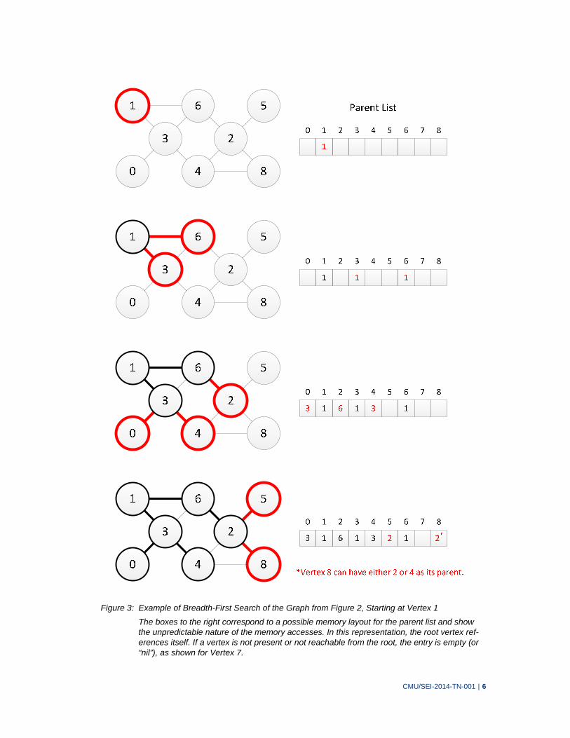
Figure 3: Example of Breadth-First Search of the Graph from Figure 2, Starting at Vertex 1

The boxes to the right correspond to a possible memory layout for the parent list and show the unpredictable nature of the memory accesses. In this representation, the root vertex ref-erences itself. If a vertex is not present or not reachable from the root, the entry is empty (or “nil”), as shown for Vertex 7.

CMU/SEI-2014-TN-001 | 7

When creating the BFS parent list, race conditions are possible, as shown in Figure 3. The Graph500 benchmark allows the implementation to treat this race as benign and does not pre-scribe a resolution. As a result, different runs or implementations can result in different solutions. Figure 3 illustrates one possible data structure output from Kernel 2, a parent list, where the par-ent in the tree for each vertex in the original graph is found by using the vertex ID to index into the list for each vertex in the graph. Once Kernel 1 is complete, 64 random roots for the BFS tree creation will be selected, and Kernel 2 will be invoked to build a BFS tree from each root. Each invocation will be timed and validated, and the number of edges from the original list that are contained in the tree will be computed. This number could differ from the total number of edges because disconnected components in the graph are possible and therefore are not reachable from the root selected.

The benchmark specifies that the performance of the algorithm must be reported for the largest scale problem that can fit into the system’s memory. While the performance of both kernels is recorded and submitted to the benchmark, the performance in Kernel 2, measured in average (harmonic mean of) traversed edges per second (TEPS), determines the ranking in the Graph500 list. Higher TEPS represent greater ability to work with a data set once placed into the desired format. Although the results of Kernel 2 are used to rank machines and architectures on the benchmark, Kernel 1 time is an important indicator for many applications where the graphs are not static. The ability to construct the graph in a timely manner allows closer to real-time capabili-ties for the graph search. Striking an effective balance between Kernel 1 and 2 is important for real-world applications. Depending on the application, faster search may be the priority and can amortize the cost to create the graph in a more traversal-efficient representation. In other cases, if Kernel 1 dominates Kernel 2, the operations on the resulting graph may be stale and not useful for the consumer.

1.3 Approach

Now that we have isolated graph creation, validation, and other invariant setup parts from the measured kernels, we can evaluate a number of different BFS algorithms. We are interested in the resulting performance of the algorithm (both Kernel 1 and Kernel 2) and some indication of the algorithm’s complexity or the level of effort involved in developing it. In Section 2, we do this for a number of hardware architectures and algorithms. The following section outlines the implemen-tations for single and multiple CPUs as well as simple and complex algorithms on GPUs. The simpler implementations serve as a baseline for our more advanced implementations. In Section 3, we examine the results of all the implementations and draw conclusions about the comparisons between each. In Section 4, we document some of the outstanding questions and problems en-countered and use this to recommend the future direction of this research.

CMU/SEI-2014-TN-001 | 8

2 Implementations

In this section, we document five different implementations of BFS across a wide spectrum of computing architectures and algorithm complexities. The first two involve sequential algorithms on a single CPU. The third implements an algorithm developed specifically for single GPUs, is run on a single NVIDIA Tesla M2090 GPU, and is restricted to problems that can fit in the GPUs’ memory. The fourth algorithm is a more ambitious approach to utilize more than one GPU pro-cess and leverage the system’s main memory to support the processing of larger scale problems. The final algorithm presented in this section uses a distributed-memory, message-passing system (the Message Passing Interface [MPI]), to abstract away the complexity of designing an algorithm for multiple CPUs. It also leverages the Combinatorial Basic Linear Algebra Subprograms (CombBLAS) library [Buluç 2014] to implement a conceptually simpler algorithm in terms of basic combinatorial linear algebra operations. We include this last algorithm to explore a recent movement in this field of research that suggests that the interface specified by these subprograms is the level of abstraction that will separate graph algorithm development from the complexities of the underlying system architecture [Mattson 2013].

To test all these implementations, we created a C++ framework that provides the functionality common to all implementations. This consists of a main program with calls to both Kernel 1 and Kernel 2 stubbed out. The framework supports the automatic generation of a graph using a Kron-ecker generator and parallel pseudo-random number generator (PRNG) that was ported from the Graph500 reference implementation. In addition, this framework has the ability to load the graph from the file system. The framework also uses the PRNG to select the roots, timer classes to measure BFS traversal time, and a statistics class to compute the overall performance of the tra-versals.

2.1 Single CPU, List

The baseline CPU implementation is a single-threaded, sequential traversal taken from Version 2.1.4 of the Graph500 reference implementation (in the “seq-list” directory). We ported the code from the provided C implementation to a C++ implementation3 and integrated it with the frame-work described above. The algorithm is broken into two steps corresponding to Kernel 1 (setup) and Kernel 2 (BFS tree generation) of the benchmark.

2.1.1 Kernel 1

In Kernel 1, all the data structures that will be used in Kernel 2 are built using the edge list as in-put. Kernel 1 of this implementation is passed the generated edge list when invoked, and it per-forms the following operations:

3 When the C++ code is built with the appropriate compiler optimization flags [-O3], there is no appreciable per-

formance difference between the executable resulting from this new implementation and the original reference C implementation.

CMU/SEI-2014-TN-001 | 9

1. Determine the largest vertex index referenced in the list (not all vertices in the graph are connected by edges) by scanning the entire edge list. This also allows determining the num-ber of edges in the list (if it is not readily apparent).

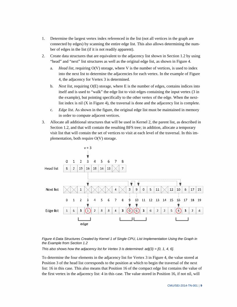
2. Create data structures that are equivalent to the adjacency list shown in Section 1.2 by using “head” and “next” list structures as well as the original edge list, as shown in Figure 4.

a. Head list, requiring O(V) storage, where V is the number of vertices, is used to index into the next list to determine the adjacencies for each vertex. In the example of Figure 4, the adjacency for Vertex 3 is determined.

b. Next list, requiring O(E) storage, where E is the number of edges, contains indices into itself and is used to “walk” the edge list to visit edges containing the input vertex (3 in the example), but pointing specifically to the other vertex of the edge. When the next-list index is nil (X in Figure 4), the traversal is done and the adjacency list is complete.

c. Edge list. As shown in the figure, the original edge list must be maintained in memory in order to compute adjacent vertices.

3. Allocate all additional structures that will be used in Kernel 2, the parent list, as described in Section 1.2, and that will contain the resulting BFS tree; in addition, allocate a temporary visit list that will contain the set of vertices to visit at each level of the traversal. In this im-plementation, both require O(V) storage.

Figure 4: Data Structures Created by Kernel 1 of Single CPU, List Implementation Using the Graph in the Example from Section 1.2

This also shows how the adjacency list for Vertex 3 is determined: adj(3) = [0, 1, 4, 6].

To determine the four elements in the adjacency list for Vertex 3 in Figure 4, the value stored at Position 3 of the head list corresponds to the position at which to begin the traversal of the next list: 16 in this case. This also means that Position 16 of the compact edge list contains the value of the first vertex in the adjacency list: 4 in this case. The value stored in Position 16, if not nil, will

CMU/SEI-2014-TN-001 | 10

indicate the next position in the next list (and the edge list) to visit. Positions 10, 9, and 3 are trav-ersed in the next list, and the corresponding entries in the edge list are added to the adjacency list: 6, 0, and 1. The complete adjacency list for Vertex 3 is [0, 1, 4, 6].

2.1.2 Kernel 2

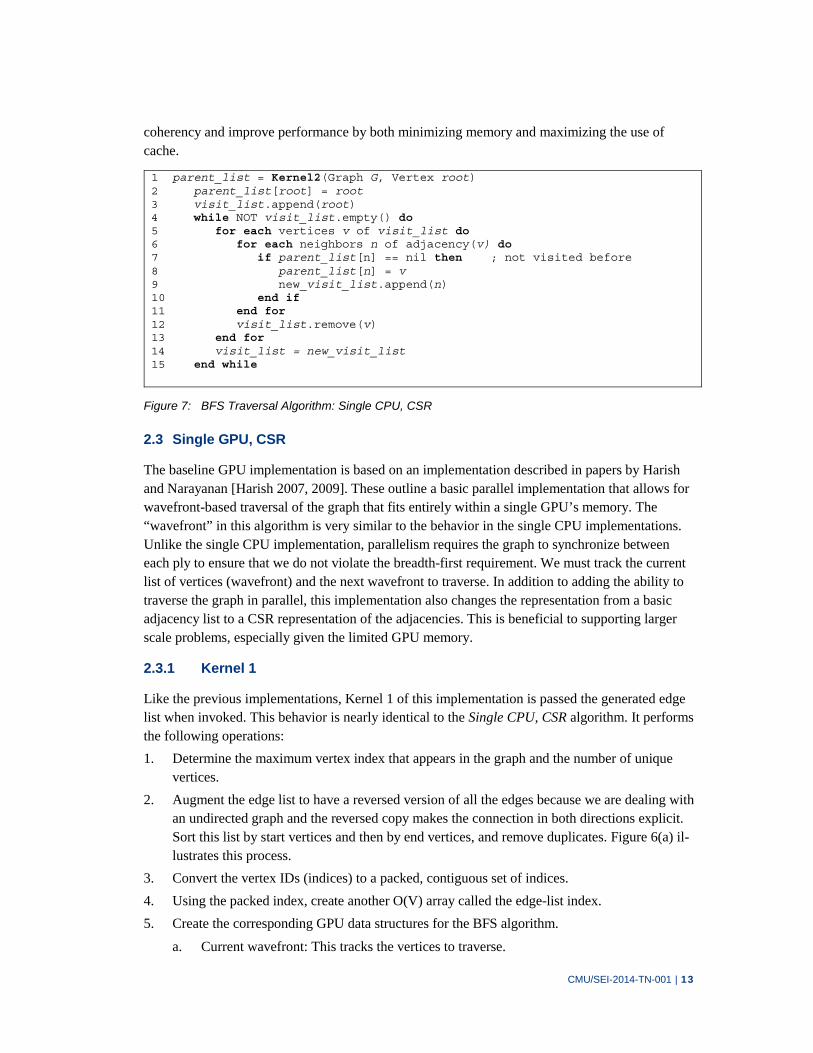
This kernel accepts a starting vertex (the root) and generates the BFS tree from this starting point. The pseudocode for the algorithm is given in Figure 5. The visit-list structure contains the list of vertices that should be visited in the next ply of the traversal. It is initialized with the root. For each vertex in the visit list, the adjacencies are determined (illustrated in Figure 4); only the verti-ces from this set that have not been visited before (they do not have a valid entry in the parent list) will be assigned the current vertex as the parent and then put on the visit list for the next level of the BFS traversal. The last level of the traversal will result in no new entries in the visit list, and the traversal ends.

1 parent_list = Kernel2(Graph G, Vertex root)2 parent_list[root] = root 3 visit_list.append(root) 4 while NOT visit_list.empty() do 5 for each vertices v of visit_list do 6 for each neighbors n of adjacency(v) do 7 if parent_list[n] == nil then ; not visited before 8 parent_list[n] = v 9 new_visit_list.append(n) 10 end if 11 end for 12 visit_list.remove(v) 13 end for 14 visit_list = new_visit_list 15 end while

Figure 5: Kernel 2 of Graph500 BFS Reference Implementation: Single CPU, List

2.2 Single CPU, Compressed Sparse Row

The adjacency-list structure of the previous section is wasteful in terms of memory usage. Be-cause the BFS graph algorithm already taxes the capabilities of the computer’s memory system, any alternative to those memory structures that uses memory more efficiently (and with more se-quential access) would show a performance improvement as well as allow larger graphs to be ma-nipulated. A data structure called the compressed sparse row (CSR) is often used in this case. This section presents the data structures that we used and the resulting BFS algorithm that we adapted from the “seq-csr” implementation in the Graph500 Reference Implementation.

2.2.1 Kernel 1

As before, all the data structures needed for the BFS algorithm are created during Kernel 1. These are built from the edge list that is passed to the routine that performs the following tasks:

1. Determine the maximum vertex index that appears in the graph and the number of unique vertices.

CMU/SEI-2014-TN-001 | 11

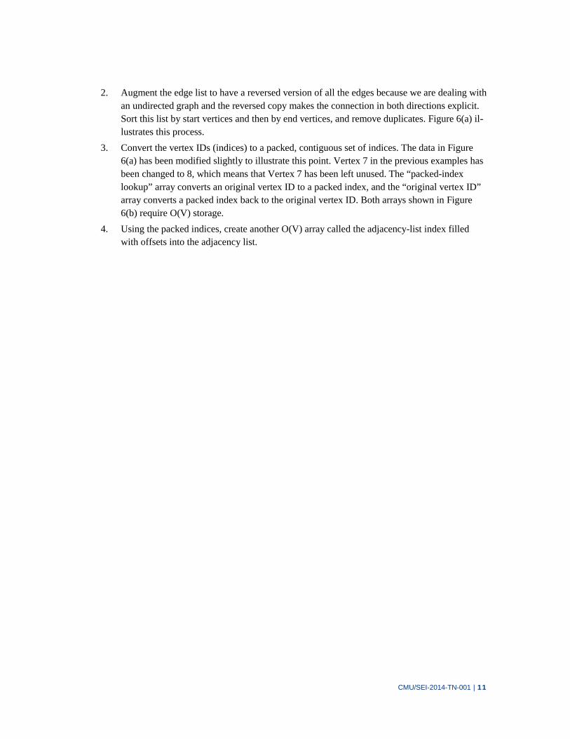
2. Augment the edge list to have a reversed version of all the edges because we are dealing with an undirected graph and the reversed copy makes the connection in both directions explicit. Sort this list by start vertices and then by end vertices, and remove duplicates. Figure 6(a) il-lustrates this process.

3. Convert the vertex IDs (indices) to a packed, contiguous set of indices. The data in Figure 6(a) has been modified slightly to illustrate this point. Vertex 7 in the previous examples has been changed to 8, which means that Vertex 7 has been left unused. The “packed-index lookup” array converts an original vertex ID to a packed index, and the “original vertex ID” array converts a packed index back to the original vertex ID. Both arrays shown in Figure 6(b) require O(V) storage.

4. Using the packed indices, create another O(V) array called the adjacency-list index filled with offsets into the adjacency list.

CMU/SEI-2014-TN-001 | 12

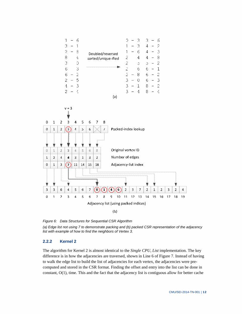
Figure 6: Data Structures for Sequential CSR Algorithm

(a) Edge list not using 7 to demonstrate packing and (b) packed CSR representation of the adjacency list with example of how to find the neighbors of Vertex 3.

2.2.2 Kernel 2

The algorithm for Kernel 2 is almost identical to the Single CPU, List implementation. The key difference is in how the adjacencies are traversed, shown in Line 6 of Figure 7. Instead of having to walk the edge list to build the list of adjacencies for each vertex, the adjacencies were pre-computed and stored in the CSR format. Finding the offset and entry into the list can be done in constant, O(1), time. This and the fact that the adjacency list is contiguous allow for better cache

CMU/SEI-2014-TN-001 | 13

coherency and improve performance by both minimizing memory and maximizing the use of cache.

1 parent_list = Kernel2(Graph G, Vertex root)2 parent_list[root] = root 3 visit_list.append(root) 4 while NOT visit_list.empty() do 5 for each vertices v of visit_list do 6 for each neighbors n of adjacency(v) do 7 if parent_list[n] == nil then ; not visited before 8 parent_list[n] = v 9 new_visit_list.append(n) 10 end if 11 end for 12 visit_list.remove(v) 13 end for 14 visit_list = new_visit_list 15 end while

Figure 7: BFS Traversal Algorithm: Single CPU, CSR

2.3 Single GPU, CSR

The baseline GPU implementation is based on an implementation described in papers by Harish and Narayanan [Harish 2007, 2009]. These outline a basic parallel implementation that allows for wavefront-based traversal of the graph that fits entirely within a single GPU’s memory. The “wavefront” in this algorithm is very similar to the behavior in the single CPU implementations. Unlike the single CPU implementation, parallelism requires the graph to synchronize between each ply to ensure that we do not violate the breadth-first requirement. We must track the current list of vertices (wavefront) and the next wavefront to traverse. In addition to adding the ability to traverse the graph in parallel, this implementation also changes the representation from a basic adjacency list to a CSR representation of the adjacencies. This is beneficial to supporting larger scale problems, especially given the limited GPU memory.

2.3.1 Kernel 1

Like the previous implementations, Kernel 1 of this implementation is passed the generated edge list when invoked. This behavior is nearly identical to the Single CPU, CSR algorithm. It performs the following operations:

1. Determine the maximum vertex index that appears in the graph and the number of unique vertices.

2. Augment the edge list to have a reversed version of all the edges because we are dealing with an undirected graph and the reversed copy makes the connection in both directions explicit. Sort this list by start vertices and then by end vertices, and remove duplicates. Figure 6(a) il-lustrates this process.

3. Convert the vertex IDs (indices) to a packed, contiguous set of indices.

4. Using the packed index, create another O(V) array called the edge-list index.

5. Create the corresponding GPU data structures for the BFS algorithm.

a. Current wavefront: This tracks the vertices to traverse.

CMU/SEI-2014-TN-001 | 14

b. Next wavefront: This tracks the adjacent vertices to traverse the next pass.

c. Visited list: This list ensures that we traverse only new sections of the graph and do not duplicate work.

d. Parent list: This list includes the results of Kernel 2 to return.

6. Copy the CSR representation to the GPU.

2.3.2 Kernel 2

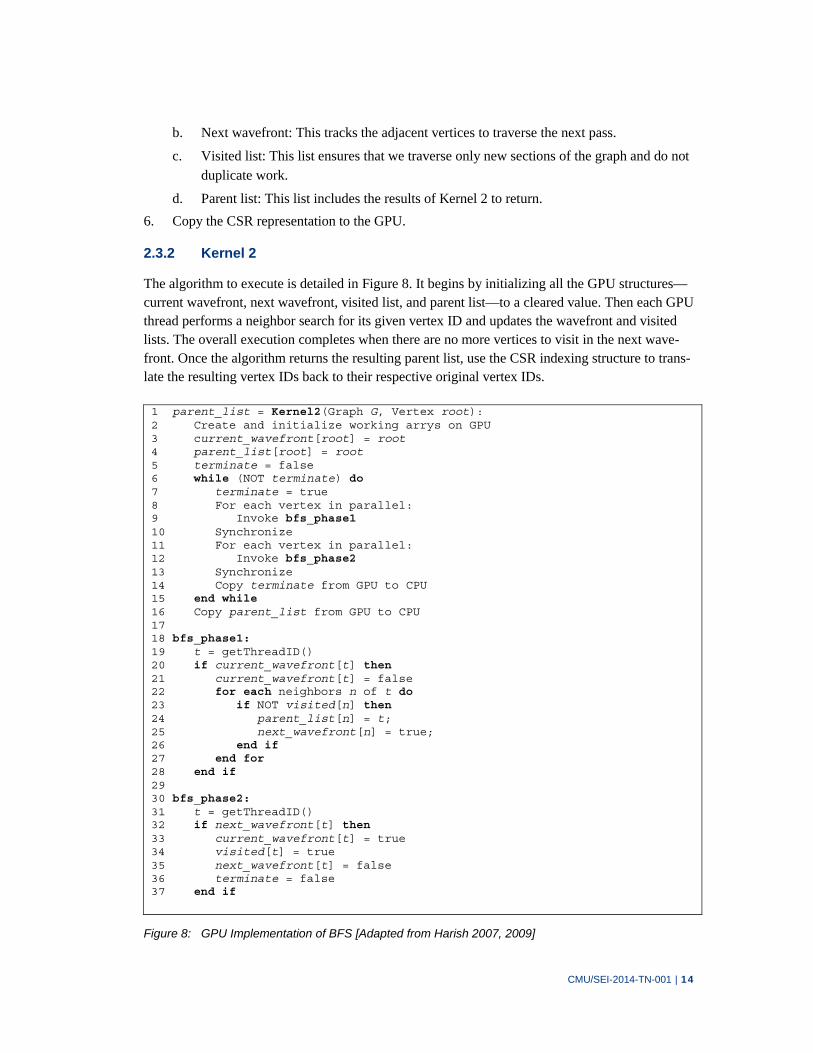
The algorithm to execute is detailed in Figure 8. It begins by initializing all the GPU structures—current wavefront, next wavefront, visited list, and parent list—to a cleared value. Then each GPU thread performs a neighbor search for its given vertex ID and updates the wavefront and visited lists. The overall execution completes when there are no more vertices to visit in the next wave-front. Once the algorithm returns the resulting parent list, use the CSR indexing structure to trans-late the resulting vertex IDs back to their respective original vertex IDs.

1 parent_list = Kernel2(Graph G, Vertex root):2 Create and initialize working arrys on GPU 3 current_wavefront[root] = root 4 parent_list[root] = root 5 terminate = false 6 while (NOT terminate) do 7 terminate = true 8 For each vertex in parallel: 9 Invoke bfs_phase1 10 Synchronize 11 For each vertex in parallel: 12 Invoke bfs_phase2 13 Synchronize 14 Copy terminate from GPU to CPU 15 end while 16 Copy parent_list from GPU to CPU 17 18 bfs_phase1: 19 t = getThreadID() 20 if current_wavefront[t] then 21 current_wavefront[t] = false 22 for each neighbors n of t do 23 if NOT visited[n] then 24 parent_list[n] = t; 25 next_wavefront[n] = true; 26 end if 27 end for 28 end if 29 30 bfs_phase2: 31 t = getThreadID() 32 if next_wavefront[t] then 33 current_wavefront[t] = true 34 visited[t] = true 35 next_wavefront[t] = false 36 terminate = false 37 end if

Figure 8: GPU Implementation of BFS [Adapted from Harish 2007, 2009]

CMU/SEI-2014-TN-001 | 15

2.4 Single GPU, Out-of-Core CSR

This approach to the BFS traversal problem focuses on splitting a given graph into many smaller subgraphs and performing BFS traversals on each smaller subgraph individually using a GPU. The final traversal of each subgraph is then stitched back together into the main graph, forming a complete BFS traversal of the original graph. The goal of breaking the main graph into smaller subgraphs allows each subgraph to be traversed individually and aids in the overall parallelizabil-ity of the algorithm. Combining it with the large number of simultaneous threads on the GPU should result in an accelerated traversal. The segmentation of graphs was intended to allow for operations on graphs that are larger than what can fit in GPU memory.

2.4.1 Kernel 1

To be effective and efficient, the algorithm proposed in this section requires the graph data to have a heavy degree of exploitable locality, which is counter to the characteristics of graphs gen-erated for the Graph500 benchmark. In Kernel 1, four steps are implemented to attempt to discov-er any locality and transform the data into a form that can be used for this algorithm. We will use the edge list in Figure 2(a) and the graph depicted in Figure 3 to illustrate each step in the process.

CMU/SEI-2014-TN-001 | 16

Figure 9: Data Structures Used in Out-of-Core GPU Algorithm

(a) Edge list from Figure 2(a). (b) Packed form of the edge list. (c) Vertex ID usage bitmap of the source edge list. Edge blocks are divided into subgraphs and may contain the edges for more than one vertex.

1. Convert the vertex IDs (indices) to a packed, contiguous set of indices. This first step trans-forms the noncontiguous vertex IDs into a contiguous set by using a packing algorithm on the input edge list. The packing process builds a vertex ID usage bitmap to identify which IDs are present in the source edge list, as shown in Figure 9(c). Use this bitmap to construct a translation table that converts the original vertex IDs into a list of packed indices that rep-resents a contiguous space (shown in the figure as “Packed-index lookup”). Derive the re-verse lookup (“Original vertex ID” in the figure), and use it to reverse the translation. Use the resulting map of packed to unpacked vertices to rewrite the input edge list into a packed form of the edge list, with every “unpacked” vertex number replaced by its “packed” coun-

CMU/SEI-2014-TN-001 | 17

terpart in Figure 9(b). The map itself is stored in two elements, packed and unpacked vertex IDs, of the VertexMap structure.

2. Compute the degree of every vertex in the graph. The degree information is also stored in the VertexMap and is used to allocate storage space for the interconnection information, called the adjacency list (next step).

3. Build the EdgeTable (adjacency list). The table consists of a set of four arrays:

Original degree of each vertex.

Degree of each vertex corresponding to the edges actually inserted into the table. This is necessary because duplicate edges and self-loops are ignored.

Offsets into the adjacency list indicating where the list of adjacent vertices starts for a specific packed vertex.

Adjacency lists for each vertex. In this array, adjacent vertices are stored in the order that they appear in the edge list. Each edge is inserted twice; the second time is the re-versed direction.

4. Construct the set of edge blocks. These blocks are groups of vertices whose collective edge lists are small enough to fit into the GPU’s global memory. Each edge block is extracted separately from data in the VertexMap, and the EdgeTable and is loaded into the memory of the GPU when necessary. Figure 9(c) shows an example of dividing the adjacency list into six edge blocks based on an arbitrary memory threshold that limits the number of adjacen-cies (plus the other edge table data for the corresponding source vertices) to no more than four. The highlighted block includes the adjacencies for two vertices.

2.4.2 Kernel 2

This algorithm uses a simple greedy algorithm applied to each edge block to determine the mini-mum possible depth for each vertex in the tree. The algorithm is shown in the pseudo-code in Figure 10.

CMU/SEI-2014-TN-001 | 18

1 parent_list = Kernel2(Graph G, Vertex root):2 Copy parent_list from CPU to GPU 3 Copy depth_list from CPU to GPU 4 terminate = false 5 while (NOT terminate) do 6 terminate = true 7 for each Vertex v in parallel: 8 Copy edge_block_list[v] from CPU to GPU ;from Kernel 1 9 Invoke bfs_kernel 10 end for 11 Synchronize 12 end while 13 Copy parent_list from GPU to CPU 14 15 bfs_kernel: 16 v = getCurrentVertex() 17 for each neighbor n in edge_block_list[v] do 18 if depth_list[n] < depth_list[v] then 19 parent_list[v] = n 20 depth_list[v] = depth_list[n] + 1 21 terminate = false 22 end if 23 end for

Figure 10: BFS Algorithm for Out-of-Core GPU Implementation

As can be seen from the algorithm, this approach focuses on each vertex reading information from its neighbors (Lines 18–22), rather than writing information to its neighbors’ storage locations. This allows for ease of parallelization across vertices and prevents collisions from multiple, sim-ultaneous writes to neighboring vertices (especially in highly connected graphs). Limiting the number of collisions is very important. Since the GPU has a loosely ordered memory model, these collisions may result in the wrong values being stored. To demonstrate this algorithm, we return to the example graph from Figure 2. Using the algorithm on our example would produce the in-termediate steps illustrated in Figure 11 when Vertex 1 is the starting vertex.

CMU/SEI-2014-TN-001 | 19

Figure 11: Steps of BFS Traversal Using the Graph from Figure 2

(a) Initial conditions, (b) after the first kernel launch, (c) after the second kernel launch, and (d) after the third kernel launch.

This result is essentially the same as for the wavefront type of traversal. Vertex 7 (Vertex 8, un-packed) could have either Vertex 2 or Vertex 4 as a parent, depending on which connecting edge is processed first. Because the edge 8 – 4 occurs after the edge 2 – 8 in the original edge list, the 8 – 4 edge would have precedence, and therefore it would be assigned Vertex 2 as the parent.

The main challenge in the execution stage is that each vertex in the source graph may have a widely varying number of edges. Each GPU kernel, for our test hardware, must be symmetric in nature, with each thread block having the same number of threads. This restriction means that a vertex with relatively few edges gets the same number of threads as one with orders of magnitude more edges.

In addition, the loosely ordered nature of memory references in our hardware presents potential hazards when updating the depth and parent of a vertex. If two threads attempt to update the depth and parent simultaneously, inconsistent outcomes are possible when the depth of one vertex is combined with the parent of another. To combat this, we used atomic operations on the shared-memory variables containing the depth and parent-vertex variables. Unfortunately, due to the way that atomic operations work, this inflicts a severe performance penalty on the normally fast shared-memory structure.

CMU/SEI-2014-TN-001 | 20

2.5 Multi-CPU, CombBLAS

Recently a large group of researchers representing the forefront of graph analytics research pre-sented a position paper that supports an effort aimed at standardizing graph algorithm primitives by using linear algebra [Mattson 2013]. Leveraging a model of past success in computing, the National Institute of Standards and Technology Sparse Basic Linear Algebra Subprograms (BLAS), the authors propose to extend the BLAS built to perform graph computations. Publica-tions such as “Graph Algorithms in the Language of Linear Algebra” [Kepner 2011], “PEGASUS: A Peta-Scale Graph Mining System” [Kang 2009], and “The Combinatorial BLAS: Design, Implementation, and Applications” [Buluç 2011] all use sparse matrices and represent graph algorithms composed of linear algebra operations. The implementation presented in this section is built on an implementation of Combinatorial BLAS, which is an “extensible distributed-memory parallel graph library offering a small but powerful set of linear algebra primitives spe-cifically targeting graph analytics” [Buluç 2014].

This implementation uses data structures for distributed sparse matrices provided by CombBLAS to represent the adjacencies in the graph and provide a way to distribute and manage concurrent accesses to the graph in the system’s memory architecture. CombBLAS also supports user-defined semi-ring operations as the method for manipulating the graph. For the BFS algorithm, this involves replacing traditional multiplication and addition operations for a matrix-vector mul-tiply with multiple and min. The CombBLAS distribution provides source code with an MPI ref-erence implementation. This has been integrated with our test framework for comparison with the other implementations. This implementation demonstrates both a multi-CPU approach and a sim-plified abstraction for attempting to perform the BFS.

2.5.1 Kernel 1

As with all other Kernel 1 implementations, input is the generated edge list. The algorithm then follows these operations:

1. Convert the edge list into an adjacency matrix. In this approach it is a distributed, parallel-ized, sparse-matrix structure.

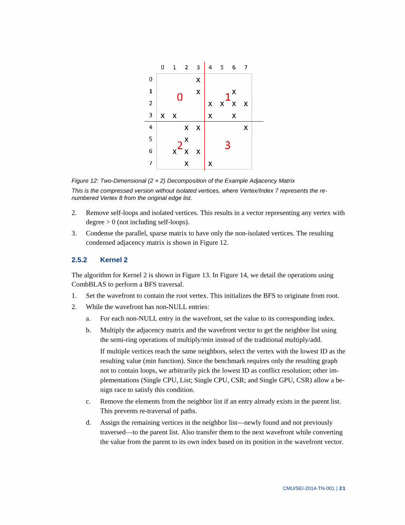
a. To distribute the computation of the graph, a two-dimensional decomposition is per-formed. Figure 12 shows a 2 × 2 example decomposition.

b. There is potential for load imbalance for both processing and vertex distribution. How-ever, well-known techniques exist for ameliorating these types of load imbalance and can mitigate the potential hot spots for computation, including random permutation, row-wise striping, jagged partitioning, and others. We used CombBLAS’s example im-plementation to dictate the partitioning scheme but disabled the random-permutation step (the vertices and edges were already randomly ordered), which also allowed for validation of the results.

CMU/SEI-2014-TN-001 | 21

Figure 12: Two-Dimensional (2 × 2) Decomposition of the Example Adjacency Matrix

This is the compressed version without isolated vertices, where Vertex/Index 7 represents the re-numbered Vertex 8 from the original edge list.

2. Remove self-loops and isolated vertices. This results in a vector representing any vertex with degree > 0 (not including self-loops).

3. Condense the parallel, sparse matrix to have only the non-isolated vertices. The resulting condensed adjacency matrix is shown in Figure 12.

2.5.2 Kernel 2

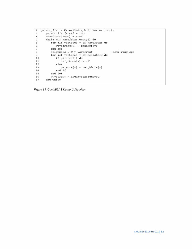
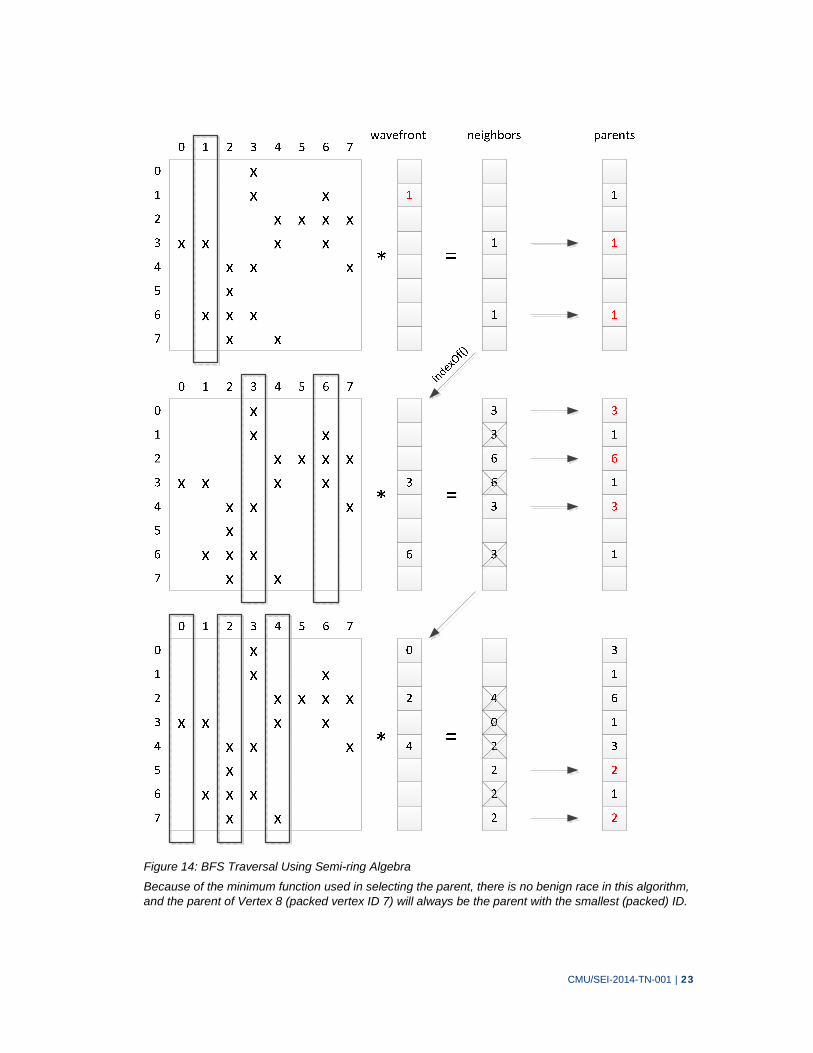
The algorithm for Kernel 2 is shown in Figure 13. In Figure 14, we detail the operations using CombBLAS to perform a BFS traversal.

1. Set the wavefront to contain the root vertex. This initializes the BFS to originate from root.

2. While the wavefront has non-NULL entries:

a. For each non-NULL entry in the wavefront, set the value to its corresponding index.

b. Multiply the adjacency matrix and the wavefront vector to get the neighbor list using the semi-ring operations of multiply/min instead of the traditional multiply/add.

If multiple vertices reach the same neighbors, select the vertex with the lowest ID as the resulting value (min function). Since the benchmark requires only the resulting graph not to contain loops, we arbitrarily pick the lowest ID as conflict resolution; other im-plementations (Single CPU, List; Single CPU, CSR; and Single GPU, CSR) allow a be-nign race to satisfy this condition.

c. Remove the elements from the neighbor list if an entry already exists in the parent list. This prevents re-traversal of paths.

d. Assign the remaining vertices in the neighbor list—newly found and not previously traversed—to the parent list. Also transfer them to the next wavefront while converting the value from the parent to its own index based on its position in the wavefront vector.

CMU/SEI-2014-TN-001 | 22

1 parent_list = Kernel2(Graph G, Vertex root):2 parent_list[root] = root 3 wavefront[root] = root 4 while NOT wavefront.empty() do 5 for all vertices v of wavefront do 6 wavefront[v] = indexOf(v) 7 end for 8 neighbors = G * wavefront ; semi-ring ops 9 for all vertices v of neighbors do 10 if parents[v] do 11 neighbors[v] = nil 12 else 13 parents[v] = neighbors[v] 14 end if 15 end for 16 wavefront = indexOf(neighbors) 17 end while

Figure 13: CombBLAS Kernel 2 Algorithm

CMU/SEI-2014-TN-001 | 23

Figure 14: BFS Traversal Using Semi-ring Algebra

Because of the minimum function used in selecting the parent, there is no benign race in this algorithm, and the parent of Vertex 8 (packed vertex ID 7) will always be the parent with the smallest (packed) ID.

CMU/SEI-2014-TN-001 | 24

3 Results for All Implementations

To evaluate the performance of our implementations, we compare performance of Kernel 1 (set-up) and Kernel 2 (BFS tree generation) across all of the implementations even though only the results in Kernel 2 are reported as the Graph500 benchmark score. Then, we use the level of effort to implement the algorithms—as estimated by source lines of code (SLOC)—to compare perfor-mance of each algorithm relative to this estimate. We tested all CPU-based implementations on an SGI UV100 system and all GPU-based implementations on systems containing NVIDIA Tesla GPUs. The appendix lists the details of these systems.

3.1 Performance Comparison of Individual Approaches

In this section, we examine the performance of both sequential and parallel algorithms. The Single GPU, CSR implementation serves as the comparative reference point between them.

3.1.1 Single CPU/GPU Performance

3.1.1.1 Kernel 1

Figure 15 shows a plot of the Kernel 1 (setup) time required for the sequential algorithms. As ex-pected, setup times for all implementations scale linearly with problem scale (asymptotically), and the simpler implementations generally take less time. The only deviation is for smaller scale prob-lems with the Single GPU, CSR implementation, where the fixed time setup for the GPU domi-nates.

Figure 15: Kernel 1 Processing Time vs. Problem Scale for All Algorithms (Lower Is Better)

CMU/SEI-2014-TN-001 | 25

3.1.1.2 Kernel 2

Kernel 2 shows some more interesting effects on performance. The driving factor behind the curves is memory access. There is a consistent ~10× difference in performance between the two sequential implementations—Single CPU, List and Single CPU, CSR—which is due to the differ-ences in memory usage of the algorithms. They both also encounter a distinct drop in performance between scales 15 and 16, which is due to the fact that the data structures needed for Kernel 2 no longer fit in the last, largest, slowest level of cache for a single CPU. The increase in cache misses and the increased cost of main-memory accesses are the reasons for the significant, negative im-pact on measured performance. The second distinct drop in performance for the Single CPU, List implementation between scale 25 and scale 26 is due to NUMA effects as the data structures no longer fit in the main memory bank directly attached to the CPU in use and spill over into memory banks that take longer to access. Since the Single GPU, CSR implementation uses a more compact graph representation, the equivalent drop should occur beyond scale 28 and is not shown on the graph in Figure 16.

Figure 16: Kernel 2 TEPS (Traversed Edges per Second) vs. Problem Scale (Higher Is Better)

The other CPU implementation reported here uses CombBLAS data structures, which are already designed to distribute the data throughout the machine. The extra complexity penalizes this im-plementation compared to the Single CPU, CSR for smaller graphs, but eventually the relatively level performance of CombBLAS results in better performance at higher scales.

The two GPU implementations, using distinctly different architectures, show poorer performance at smaller scales and better performance as the problem size increases and utilize the GPU’s cores more efficiently. Although these are single GPU implementations, they are multiple-core algo-rithms and are included here for comparison.

CMU/SEI-2014-TN-001 | 26

3.1.2 Parallel CPU/GPU Performance

3.1.2.1 Kernel 1

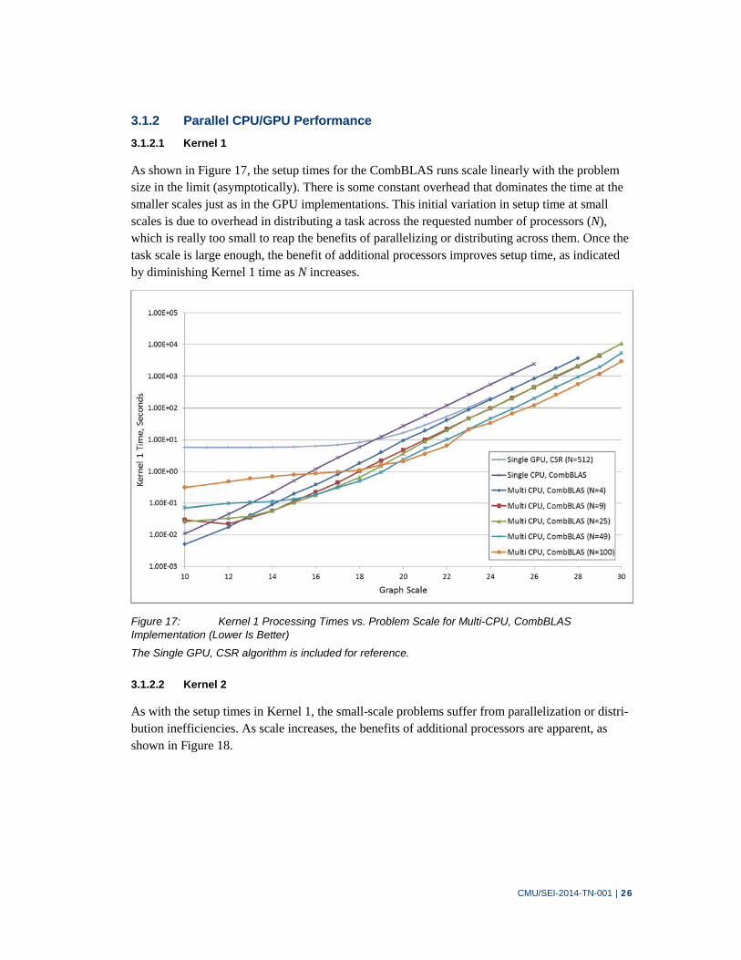
As shown in Figure 17, the setup times for the CombBLAS runs scale linearly with the problem size in the limit (asymptotically). There is some constant overhead that dominates the time at the smaller scales just as in the GPU implementations. This initial variation in setup time at small scales is due to overhead in distributing a task across the requested number of processors (N), which is really too small to reap the benefits of parallelizing or distributing across them. Once the task scale is large enough, the benefit of additional processors improves setup time, as indicated by diminishing Kernel 1 time as N increases.

Figure 17: Kernel 1 Processing Times vs. Problem Scale for Multi-CPU, CombBLAS Implementation (Lower Is Better)

The Single GPU, CSR algorithm is included for reference.

3.1.2.2 Kernel 2

As with the setup times in Kernel 1, the small-scale problems suffer from parallelization or distri-bution inefficiencies. As scale increases, the benefits of additional processors are apparent, as shown in Figure 18.

CMU/SEI-2014-TN-001 | 27

Figure 18: Kernel 2 TEPS (Traversed Edges per Second) vs. Problem Scale (Higher Is Better)

3.2 Performance vs. Code Complexity

Because one of the key goals of this research is to define the abstractions that make the construc-tion of graph algorithms much easier while not sacrificing performance, this section examines the effort that was required to develop the implementations against their performance achieved in Kernel 2. We use SLOC as a proxy for effort and maintenance estimation [Humphrey 2005]. We used the “cloc” utility [Danial 2013] to gather SLOC for each implementation, and Table 1 lists the results. All code that is common to all implementations (parallel PRNG, graph generation, timing, validation of results, etc.) is part of our common evaluation framework and is not included here.

Table 1: Comparison of Implementation Source Lines of Code

Implementation Non-framework SLOC

Single CPU, List 135

Single CPU, CSR 179

Single GPU, CSR 217

Single GPU, Out-of-Core CSR 1,932

Multi-CPU, CombBLAS 190

In Figure 19, the SLOC is normalized to the simplest implementation, Single CPU, List, and the resulting relative levels of effort for each implementation are plotted against its performance of Kernel 2 for the largest scale problem that was run on the system. With the CombBLAS imple-mentation, all multiprocessing levels are achieved with the same code and hence the same level of effort, and the use of multiple processors achieves performance levels that are above the trend. At

CMU/SEI-2014-TN-001 | 28

the same time, the Single GPU, Out-of-Core CSR implementation is extremely complex and the resulting performance is well below the trend. The hope is that the implementation will compare favorably to other out-of-core algorithms, which pay extreme penalties for data access that is off the device (either in CPU main memory or disk storage).

Figure 19: Kernel 2 TEPS vs. Normalized Level of Effort (Scaled to Single CPU, List SLOC)

3.3 Summary

The initial BFS algorithms were implemented to study their effects on the CPU and main-memory architectures. Performance measurements showed that the Single CPU, List algorithm, which had the shortest Kernel 1 (setup) times, had the poorest performance on Kernel 2 (the BFS tree gen-eration). It reused the edge list to build the adjacency list through an array of indices and offsets into this edge list. The resulting pattern of memory accesses not only taxed the memory system when the graphs did not fit into cache (at scales above 15), it also resulted in relatively poor cache-system performance when the entire graph fit into the largest, slowest level of cache (at scales below 16) because it was still taxing the performance of the smallest, fastest levels of cache. By contrast, the Single CPU, CSR implementation, which spent an order of magnitude more time in Kernel 1 to build the graph structures, capitalized on the cache-friendly nature of its computed adjacency list. Each vertex has direct access to a list of its adjacent vertices, each of which is placed in contiguous memory, which allows for better performance even in the smaller, faster caches.

The Single GPU, CSR implementation incurred additional input/output (I/O) costs to transfer the data between the GPU and CPU. At smaller scales, the additional I/O hindered the measured per-

CMU/SEI-2014-TN-001 | 29

formance. To take full advantage of the GPU’s SIMD-optimized architecture, the transfer times between CPU and GPU should be amortized by the computation time. Similar to the performance difference between cache and memory, the GPU has its own hierarchy of memory and costs to move data within the GPU and within the broader heterogeneous environment. Accounting for these costs is vital to creating high-performance solutions.

The Single GPU, Out-of-Core CSR implementation demonstrates how I/O access inefficiencies can detrimentally affect performance. In an attempt to divide the work into discrete, parallelizable chunks, we inadvertently segmented computation in such a way as to require additional commu-nication, relative to the other implementations, between traversals. As before, the additional I/O hampered the overall performance of the algorithm, despite the GPU’s demonstrated capability to outperform the single CPU implementations.

Finally, the implementation built on the CombBLAS library results in the best performance on multi-CPU systems with a reasonable amount of effort. Advantages of this approach are that it provides a number of data structures necessary for many graph computations and hides from the developer the complexity of the management of multithreading and distributing these data struc-tures throughout a system. Because it is a lower level abstraction, it does not implement graph algorithms. Also there are currently no implementations on GPU. Given the position of many leading researchers in the graph analytics field [Mattson 2013], however, the linear algebra im-plemented by the CombBLAS library may represent the correct level of abstraction to separate the concerns of implementing graph algorithms (on top of the library) from the concerns of the hard-ware and implementing memory-efficient abstractions and data structures (within the library).

CMU/SEI-2014-TN-001 | 30

4 Conclusions and Future Work

For this project, we implemented a number of different algorithms to compute a basic graph struc-ture: the BFS tree. The low compute-to-I/O (memory access) ratio of this algorithm is characteris-tic of many other graph algorithms. This and the unpredictable nature of the memory accesses are primary reasons this particular algorithm is included in the Graph500 benchmark. Studying the performance of various implementations of this algorithm can give insight into the performance of a system’s memory architecture when dealing with large graphs and many other typical graph algorithms.

The impact of memory I/O performance on overall algorithm performance emphasizes the need to separate concerns of the hardware from the high-level algorithms. This approach was taken over 40 years ago with the introduction of libraries like BLAS for compute-intensive, numerical appli-cations, as shown on the left side of Figure 20. BLAS defined an interface consisting of basic data structures and operations. This was usually highly tuned for specific computer systems and pro-vided by the companies that built the systems. Applications were written against this interface and other libraries built on BLAS such as LINPACK, and later LAPACK, for high-performance nu-merical codes. This division of concerns is also reflected in the position paper on graph primitives by Mattson and colleagues [Mattson 2013] and in the related work on the CombBLAS library [Buluç 2011, 2014].

Figure 20: Comparison of Linear Algebra (left) and the Proposed Graph Analytics (right) Library Architectures

The libraries (shaded) provide an interface/abstraction layer between the hardware and application layers. Within the library design is an interface that represents the separation of concerns between hardware and graph algorithms.

Similarly, an interface consisting of basic structures and operations necessary to support algo-rithms in the graph analytics space must be defined. To aid in its definition, we must determine what constitutes a sufficient set of graph algorithms and whether or not they can be represented by the linear algebra abstraction of something like CombBLAS, an abstraction found in one of the other graph libraries (Parallel Boost Graph Library [PBGL], MultiThreaded Graph Library, etc.), or some combination.

Once this abstraction layer is established, the effort forks into developing two library layers, as shown on the right side of Figure 20. Below the dotted line, developers familiar with the hardware can develop optimized, low-level implementations of these structures and operations for specific

CMU/SEI-2014-TN-001 | 31

hardware. Some libraries currently in use at this level of abstraction include MPI and Active Mes-sages++ (AM++) for memory abstractions and CombBLAS for data abstractions. Above this line, developers who understand graph analytics can then more easily compose portable algorithms building on these highly optimized data structures operations, such as those found in the Boost Graph Library, PBGL, and similar offerings. By decoupling these concerns, greater advances can be achieved in both domains, rather than spreading the developers’ efforts across domains in which they may not be as familiar.

While most of the work in this area has been directed at multi-CPU and distributed CPU systems, accelerators appear to have potential for positively affecting the performance graph analytics space and are addressed in follow-on work. Although this includes offerings such as Intel’s Xeon Phi and Tilera TILE processors, we will focus on developing support for GPU accelerators whose inclusion in such HPC systems is on the rise. With a successful library implementation, the archi-tecture found in GPUs will be more easily utilized when developing future graph analytic sys-tems.

CMU/SEI-2014-TN-001 | 32

Appendix Test Hardware Configuration

CPU-Only Configuration

SGI UV 100

1 TB of RAM

128 cores: 16 × 8-core Intel Xeon E7-8837 2.67-GHz processors

This system is illustrated in Figure 21 and consists of four node cards. A node card consists of two compute blades, each with two 8-core Xeon CPUs with 24 MB of L3 cache, as shown in Figure 21(a). One 64 GB bank of shared main memory is directly connected to each Xeon. A UV Hub chip provides four NUMALink 5 (NL5) connections to other blades. One of these NL5 connec-tions is dedicated to a connection to the other blade on the node card (shown in red). Two inter-connect topologies are supported with eight blades. Figure 21(b) shows a 2 × 4 torus with double connections (red and green) between blades of a node card, and Figure 21(c) shows a three-

dimensional (3-D) hypercube with connections across the diagonals (green).

CMU/SEI-2014-TN-001 | 33

L3 = 24MB

L3 = 24MB

L3 = 24MB

L3 = 24MB

Figure 21: SGI UV 100 (CPU-Only) Configuration

(a) A single node card consisting of two blades. Two interconnect topologies are supported with four node cards: (b) a 2 x 4 torus (3 hops max) and (c) a 3-D hypercube with express links (2 hops max).

CMU/SEI-2014-TN-001 | 34

GPU Host Configuration

The GPU host configuration is illustrated in Figure 22 and consists of the following hardware:

SGI C2108 2U server

48 GB of RAM in two banks

two 4-core Intel Xeon E5620 2.40-GHz processors (8 cores, 16 threads)

two NVIDIA Tesla M2090 each with

1 Fermi GPU

6-GB GDDR5 memory

16 multiprocessors × 32 CUDA cores/MP = 512 CUDA cores

665-GFLOPs peak double-precision performance

1,331-GFLOPs peak single-precision performance

Figure 22: SGI C2108 2U Server with Two NVIDIA Tesla GPUs

CMU/SEI-2014-TN-001 | 35

5 References

URLs are valid as of the publication date of this document.

[Bader 2005] Bader, David A. & Kamesh Madduri. “Design and Implementation of the HPCS Graph Analysis Benchmark on Symmetric Multiprocessors,” 465–476. Lecture Notes in Computer Science: High Performance Computing–HiPC 2005, vol. 3769. Springer, 2005.

[Bader 2006] Bader, David A.; Feo, John; Gilbert, John; Kepner, Jeremy; Koester, David; & Loh, Eugene. HPCS Scalable Synthetic Compact Applications #2: Graph Analysis (Version 2). GraphAnaly-sis.org (2006).

[Buluç 2011] Buluc, Aydin & Gilbert, John R. “The Combinatorial BLAS: Design, Implementation, and Appli-cations.” International Journal of High Performance Computing Applications 25, 4 (Nov. 2011): 496–509.

[Buluç 2014] Buluç, Aydın; Gilbert, John R.; Lugowski, Adam; & Beamer, Scott. Combinatorial BLAS Li-brary. http://gauss.cs.ucsb.edu/~aydin/CombBLAS/html (2014).

[Danial 2013] Danial, Al. CLOC: Count Lines of Code. Northrop Grumman Corporation, 2006–2013. http://cloc.sourceforge.net

[Fuller 2011] Fuller, Samuel H. & Millet, Lynette I., eds., National Research Council. The Future of Computing Performance: Game Over or Next Level? National Academies Press, 2011.

[Graph500 2011] Graph500. Graph500 Benchmark. http://www.graph500.org (2011).

[Harish 2007] Harish, Pawan & Narayanan, P. J. “Accelerating Large Graph Algorithms on the GPU Using CUDA,” 197–208. Lecture Notes in Computer Science: High Performance Computing–HiPC 2007, vol. 4873. Springer, 2007.

[Harish 2009] Harish, Pawan; Vineet, Vibhav; & Narayanan, P. J. Large Graph Algorithms for Massively Multi-threaded Architectures (Tech. Rep. IIT/TR/2009/74). Centre for Visual Information Technology, India Institute of Technology, Hyderabad, India, 2009.

CMU/SEI-2014-TN-001 | 36

[Humphrey 2005] Humphrey, Watts S. PSP: A Self-Improvement Process for Software Engineers. Addison-Wesley Professional, 2005.

[Kang 2009] Kang, U.; Tsourakakis, Charalampos E.; & Faloutsos, Christos. “Pegasus: A Peta-Scale Graph Mining System Implementation and Observations,” 229–238. In Proceedings of ICDM 2009: The Ninth IEEE International Conference on Data Mining. Miami, FL, Dec. 2009. IEEE Computer Society Press, 2009.

[Kepner 2011] Kepner, Jeremy & Gilbert, John, eds. Graph Algorithms in the Language of Linear Algebra, vol. 22. Society for Industrial and Applied Mathematics, 2011.

[Mattson 2013] Mattson, Tim, et al. “Standards for Graph Algorithm Primitives.” Presented at the 2013 IEEE High Performance Extreme Computing Conference. Waltham, MA, Sep. 2013. http://www.netlib.org/utk/people/JackDongarra/PAPERS/GraphPrimitives-HPEC.pdf

[Moore 1965] Moore, Gordon E. “Cramming More Components onto Integrated Circuits.” Electronics 38, 8 (Apr. 1965): 114–117.

[Murphy 2010] Murphy, Richard C.; Wheeler, Kyle B.; Barrett, Brian W.; & Ang, James A. Introducing the Graph500. Cray User Group, May 2010.

[Seshadhri 2011] Seshadhri, C.; Pinar, A.; & Kolda, T. G. “A Hitchhiker’s Guide to Choosing Parameters of Sto-chastic Kronecker Graphs.” http://arxiv.org/abs/1102.5046v1 (2011).

[Sutter 2005] Sutter, Herb. “A Fundamental Turn Toward Concurrency in Software.” Dr. Dobb’s Journal 30, 3 (Mar. 2005): 202–210.

[Sutter 2009] Sutter, Herb. The Free Lunch Is Over: A Fundamental Turn Toward Concurrency in Software. http://www.gotw.ca/publications/concurrency-ddj.htm (2009).

CMU/SEI-2014-TN-001 | 37

REPORT DOCUMENTATION PAGE Form Approved OMB No. 0704-0188

Public reporting burden for this collection of information is estimated to average 1 hour per response, including the time for reviewing instructions, search-ing existing data sources, gathering and maintaining the data needed, and completing and reviewing the collection of information. Send comments regard-ing this burden estimate or any other aspect of this collection of information, including suggestions for reducing this burden, to Washington Headquarters Services, Directorate for information Operations and Reports, 1215 Jefferson Davis Highway, Suite 1204, Arlington, VA 22202-4302, and to the Office of Management and Budget, Paperwork Reduction Project (0704-0188), Washington, DC 20503.

1. AGENCY USE ONLY

(Leave Blank)

2. REPORT DATE

August 2014

3. REPORT TYPE AND DATES COVERED

Final

4. TITLE AND SUBTITLE

Patterns and Practices for Future Architectures

5. FUNDING NUMBERS

FA8721-05-C-0003

6. AUTHOR(S)

Eric Werner, Scott McMillan, and Jonathan Chu

7. PERFORMING ORGANIZATION NAME(S) AND ADDRESS(ES)

Software Engineering Institute Carnegie Mellon University Pittsburgh, PA 15213

8. PERFORMING ORGANIZATION REPORT NUMBER

CMU/SEI-2014-TN-001

9. SPONSORING/MONITORING AGENCY NAME(S) AND ADDRESS(ES)

AFLCMC/PZE/Hanscom

Enterprise Acquisition Division

20 Schilling Circle

Building 1305

Hanscom AFB, MA 01731-2116

10. SPONSORING/MONITORING AGENCY REPORT NUMBER

n/a

11. SUPPLEMENTARY NOTES

12A DISTRIBUTION/AVAILABILITY STATEMENT

Unclassified/Unlimited, DTIC, NTIS

12B DISTRIBUTION CODE

13. ABSTRACT (MAXIMUM 200 WORDS)

Graph algorithms are widely used in Department of Defense applications including intelligence analysis, autonomous systems, cyber in-telligence and security, and logistics optimization. These analytics must execute at larger scales and higher rates to accommodate the growing velocity, volume, and variety of data sources. The implementations of these algorithms that achieve the highest levels of per-formance are complex and intimately tied to the underlying architecture. New and emerging computing architectures require new and dif-ferent implementations of these well-known graph algorithms, yet it is increasingly expensive and difficult for developers to implement algorithms that fully leverage their capabilities. This project investigates approaches that will make high-performance graph analytics on new and emerging architectures more accessible to users. The project is researching the best practices, patterns, and abstractions that will enable the development of a software graph library that separates the concerns of expressing graph algorithms from the details of the underlying computing architectures. The approach started with a fundamental graph analytics function: the breadth-first search (BFS). This technical note compares different BFS algorithms for central and graphics processing units, examining the abstractions used and comparing the complexity of the implementations against the performance achieved.

14. SUBJECT TERMS

computing architecture, graph algorithms, high-performance computing, big data, GPU

15. NUMBER OF PAGES

44

16. PRICE CODE

17. SECURITY CLASSIFICATION OF REPORT

Unclassified

18. SECURITY CLASSIFICATION OF THIS PAGE

Unclassified

19. SECURITY CLASSIFICATION OF ABSTRACT

Unclassified

20. LIMITATION OF ABSTRACT

UL NSN 7540-01-280-5500 Standard Form 298 (Rev. 2-89) Prescribed by ANSI Std. Z39-18

298-102