Pattern Recognition Letters 40 (2014) 104–112

Contents lists available at ScienceDirect

Pattern Recognition Letters

journal homepage: www.elsevier .com/locate /patrec

Integration of dense subgraph finding with feature clusteringfor unsupervised feature selection q

0167-8655/$ - see front matter � 2013 Elsevier B.V. All rights reserved.http://dx.doi.org/10.1016/j.patrec.2013.12.008

q This paper has been recommended for acceptance by S. Sarkar.⇑ Corresponding author. Tel.: +91 33 2575 3114; fax: +91 33 2578 3357.

E-mail addresses: sanghami@isical.ac.in (S. Bandyopadhyay), tapas.bhadra@isical.ac.in (T. Bhadra), pabitra@cse.iitkgp.ernet.in (P. Mitra), umaulik@cse.jdvu.ac.in (U. Maulik).

Sanghamitra Bandyopadhyay a,⇑, Tapas Bhadra a, Pabitra Mitra b, Ujjwal Maulik c

a Machine Intelligence Unit, Indian Statistical Institute, Kolkata 700108, Indiab Department of Computer Science and Engineering, Indian Institute of Technology, Kharagpur 721302, Indiac Department of Computer Science and Engineering, Jadavpur University, Kolkata 700032, India

a r t i c l e i n f o

Article history:Received 15 May 2013Available online 15 December 2013

Keywords:Pattern recognitionUnsupervised feature selectionMutual informationNormalized mutual information

a b s t r a c t

In this article a dense subgraph finding approach is adopted for the unsupervised feature selection prob-lem. The feature set of a data is mapped to a graph representation with individual features constitutingthe vertex set and inter-feature mutual information denoting the edge weights. Feature selection is per-formed in a two-phase approach where the densest subgraph is first obtained so that the features aremaximally non-redundant among each other. Finally, in the second stage, feature clustering aroundthe non-redundant features is performed to produce the reduced feature set. An approximation algorithmis used for the densest subgraph finding. Empirically, the proposed approach is found to be competitivewith several state of art unsupervised feature selection algorithms.

� 2013 Elsevier B.V. All rights reserved.

1. Introduction

Over the past decade pattern recognition techniques have beenextensively used to solve several real-life problems that involvevery high dimensional data. Dimensionality reduction is almost al-ways necessary to remove the redundant features while retainingthe salient characteristics of the data as far as possible (Kwakand Choi, 2002).

Feature selection algorithms can be divided into two categoriesbased on the feature evaluation methodology, namely, filter andwrapper methods (Dash and Liu, 1997). In the filter approaches,a candidate feature subset is evaluated at each iteration based oncertain statistical measures. Some known filter type approachesare based on t-test (Hua et al., 2008), chi-square test (Jin et al.,2006), Wilcoxon Mann–Whitney test (Liao et al., 2007), mutualinformation (Battiti, 1994; Kwak and Choi, 2002; Peng et al.,2005; Estévez et al., 2009; Vinh et al., 2010), Pearson correlationcoefficients (Biesiada and Duch, 2008), etc. On the other hand,wrapper methods utilize the performance of a classifier as the eval-uation criteria for measuring the goodness of a candidate featuresubset (Kohavi and John, 1997).

Based on the availability of class labels, feature selection algo-rithms can also be classified in two ways, namely, supervisedand unsupervised feature selection. Supervised feature selection

is generally employed when the class information are in hand,otherwise unsupervised approach is used. Most known filter typeapproaches, belong to the category of supervised learning. On theother hand, a limited number of researches have been conductedin the field of unsupervised feature selection. Unsupervised featureselection using feature similarity measure (FSFS) (Mitra et al.,2002), Laplacian Score for Feature Selection (LSFS) (He et al.,2005), SPectral Feature Selection (SPFS) (Zhao and Liu, 2007), MultiCluster Feature Selection (MCFS) (Cai et al., 2010), UnsupervisedDiscriminative Feature Selection (UDFS) (Yang et al., 2011), etc.are some existing algorithms in this domain.

Feature selection is inherently a combinatorial optimizationproblem (Kohavi and John, 1997). Conventional feature selectionmethods usually follow a greedy approach and choose top-rankingfeatures on an individual level. This ignore the mutual dependencyamong the selected features. As a result of this, the optimal featuresubset is sometimes difficult to find. The above mentioned fiveunsupervised feature selection algorithms except MCFS and UDFSfollow the same methodology for obtaining the reduced featureset.

We attempt to incorporate the combinatorial effect, by adopt-ing a graph theoretic approach utilising the notion of densest sub-graph. The subgraph finding task is a known problem for a diversenumber of applications like community mining, web mining, com-putational biology (Bahmani et al., 2012). Densest subgraph find-ing is a NP-hard problem. Recently, approximation algorithms forfinding the densest subgraph have been devised in literature(Bahmani et al., 2012). Finding a subset of representative featuresby mining dense subgraph has also been addressed in Liu et al.

S. Bandyopadhyay et al. / Pattern Recognition Letters 40 (2014) 104–112 105

(2011) and Mandal and Mukhopadhyay (2013). Liu et al. (2011)proposed a supervised method for obtaining the most informativefeatures while Mandal and Mukhopadhyay (2013) used an unsu-pervised approach for obtaining the minimally redundant features.Here we have developed a new unsupervised feature selectiontechnique based on the principle of densest subgraph finding fol-lowed by feature clustering.

We first obtain a graph representation by considering the entirefeature set as the vertex set and having the inter-feature similarityas the corresponding edge weight. Here, the inter-feature similar-ity is computed using a normalized form of mutual information.

The densest subgraph finding approach has one major advan-tage that the vertices of this densest subgraph, i.e., the featuresof the reduced feature set, will be highly dissimilar. However, itis likely that these features may not be the optimal feature set.The reason behind this is that these features may not be the bestrepresentatives of the features that have been excluded, eventhough they are highly dissimilar to each other. To overcome thissituation, a clustering approach is further applied on this densestsubgraph for obtaining a better subgraph so that no important fea-ture can be excluded from this set. The variance is used in the clus-tering phase to select the prototype feature while the samenormalized mutual information is utilized for assigning eachnon-selected feature into its closest cluster representative. Thesubgraph thus obtained essentially contains a subset of the originalfeatures that can maximally represent the entire feature space.Thus our approach proceeds in a two-phase manner in which thefirst phase deals with finding out the densest subgraph while clus-tering the subgraph is performed in the second.

The remaining part of the paper is organized as follows:Section 2 discusses some preliminary concepts following whichsome of the existing unsupervised feature selection algorithmsare discussed in Section 3. The proposed two-phase unsupervisedfeature selection algorithm is described in Section 4. Subsequently,the experiential design and the comparative results are provided inSection 5. Finally, some concluding comments are made inSection 6.

2. Preliminary concepts

This section describes some fundamental information andgraph theory measures.

2.1. Density of a subgraph

Let G ¼ ðV ; EÞ be an unweighted undirected graph. The densityof a subgraph S # V , denoted as dðSÞ, is defined as dðSÞ ¼ jEðSÞjjSj , where

EðSÞ is the induced edge set of the subgraph S and jSj is the cardi-nality of S.

The maximum density of the graph, denoted as d�ðGÞ, is definedas d�ðGÞ ¼maxS # VfdðSÞg. Similarly, the density of a subgraph S # Vwithin a weighted graph G ¼ ðV ; EÞ can also be defined as

dðSÞ ¼P

e2EðSÞwe

jSj , where EðSÞ is the induced edge set of the subgraph

S and we is the weight of the edge e 2 EðSÞ.

2.2. Mutual information measures

2.2.1. EntropyEntropy of a random variable is the amount of uncertainty asso-

ciated with it (Cover and Thomas, 2012). The entropy of a discretevariable X, denoted by HðXÞ, is defined as

HðXÞ ¼ �Xx2X

pðxÞlogbpðxÞ; ð1Þ

where pðxÞ indicates the probability mass function of X. The value ofb is generally assumed to be 2:0 and this value is used in the presentpaper.

2.2.2. Mutual informationMutual information between two random variables measures

how much information can be extracted through the knowledgeof the other (Cover and Thomas, 2012). The value of mutual infor-mation becomes zero when the associated variables are completelyindependent whereas its higher value signifies their high mutualdependency. The mutual information between two discrete vari-ables X and Y, denoted as IðX; YÞ, is defined as follows

IðX; YÞ ¼Xx2X

Xy2Y

pðx; yÞlogbpðx; yÞ

pðxÞpðyÞ

� �; ð2Þ

where pðxÞ;pðyÞ and pðx; yÞ denote the probability mass function ofX, the probability mass function of Y and the joint probability massfunction between X and Y, respectively.

2.2.3. Normalized mutual informationMutual information has a disadvantage due to its non-compara-

bility among variable pairs that have different mutual informationvalues in various ranges. To overcome this, mutual information isoften normalized into a closed interval, say [0;1].

Several researchers have used various methods to constructnormalized mutual information. A few of them are mentionedbelow

I�ðX;YÞ ¼ 2IðX; YÞ

HðXÞ þ HðYÞ ; ð3Þ

IðX;YÞ ¼ IðX; YÞminðHðXÞ;HðYÞÞ ; ð4Þ

I0ðX;YÞ ¼ IðX; YÞffiffiffiffiffiffiffiffiffiffiffiffiffiffiffiffiffiffiffiffiffi

HðXÞHðYÞp : ð5Þ

Witten and Frank (2005) proposed the first one, known as symmet-ric uncertainty in the form of the weighted average of the twouncertainty coefficients. Strehl and Ghosh (2002) favoured the thirdform over the second one for ensembling several clusters due to thecloseness to a normalized inner product in Hilbert space.

3. Review of unsupervised feature selection

Many of the earlier feature selection algorithms are based onsupervised learning. Among the unsupervised feature selection ap-proaches, data variance is the simplest measure for evaluating thediscriminating power of a feature.

In the context of unsupervised feature selection algorithm, FSFS,proposed by Mitra et al. (2002), is a popular one. In this work, Mitraet al. (2002) proposed a new similarity measure, known as Maxi-mal Information Compression Index (MICI) that was used to itera-tively remove some number of features, say k, decrementing k untilno removal was possible. The MICI between two variables x and y,denoted by k2ðx; yÞ, was defined as follows

k2ðx; yÞ ¼ ðvarðxÞ þ varðyÞÞ

�ffiffiffiffiffiffiffiffiffiffiffiffiffiffiffiffiffiffiffiffiffiffiffiffiffiffiffiffiffiffiffiffiffiffiffiffiffiffiffiffiffiffiffiffiffiffiffiffiffiffiffiffiffiffiffiffiffiffiffiffiffiffiffiffiffiffiffiffiffiffiffiffiffiffiffiffiffiffiffiffiffiffiffiffiffiffiffiffiffiffiffiffiffiffiffiffiffiffiffiffiffiffiffiffiðvarðxÞ þ varðyÞÞ2 � 4varðxÞvarðyÞð1� qðx; yÞ2Þ

q;

ð6Þ

where var(x), var(y) and qðx; yÞ denote the variance of x, the vari-ance of y, and the correlation coefficient between x and y,respectively.

A benefit of the approach is that it does not require any searchwhich in turn makes the selection problem fast. However, this

106 S. Bandyopadhyay et al. / Pattern Recognition Letters 40 (2014) 104–112

approach has a major drawback regarding choosing the proper va-lue for k.

Laplacian Score for Feature Selection (LSFS) is another featureselection algorithm that is designed for serving both supervisedand unsupervised learning (He et al., 2005). Like any other filtertype approach, LSFS selects some top-ranking features that havemaximum locality preserving power computed in terms of Lapla-cian score. The motivation behind LSFS is that two closest datapoints are likely to be in the same class. The underlying idea forthis is that the local structure of the data is given more priorityover the global structure for several classification problems likeK-NN rule, etc.

SPectral Feature Selection (SPFS), designed using spectral graphtheory, is one of the first research works where a general frame-work of feature selection is proposed for both supervised as wellas unsupervised learning. This work deals with capturing the struc-tural information of a graph from the corresponding spectrum. Inthis study, the spectrum of the graph is used to measure the fea-ture relevance. Furthermore, two existing feature selection algo-rithms, namely, ReliefF (supervised) (Kononenko, 1994) and LSFS(unsupervised), have been derived as a special case of thisframework.

All of these algorithms consider the feature importance individ-ually and finally choose some user defined number of features asthe reduced feature set. The main problem of these approaches isthat the mutual relationship among the selected features is notmodeled adequately. To overcome this problem, MCFS is designedby incorporating spectral clustering analyzes of the data (manifoldlearning) with L1-regularized models (Cai et al., 2010). The mainmotivation of using spectral analysis technique here is to effi-ciently compute the correlations among different features of a can-didate feature subset in an unsupervised manner. So identifyingthe multi-cluster data structure is a major advantage of thisapproach. Here the optimization problem related to featureselection is effectively solved by employing a sparse eigen-problemas well as a L1-regularized least squares problem.

Unsupervised Discriminative Feature Selection (UDFS) is a veryrecently proposed unsupervised feature selection algorithm basedon the joint effect of discriminative analysis and L2;1-norm minimi-zation. Similar to MCFS, UDFS also analyzes features collectively ina batch mode. Additionally, UDFS exploits the discriminativepower of a feature set along with considering the local structureof data distribution.

4. Proposed feature selection technique

We attempt to model the feature selection and dependencymodeling problem using a graph theoretic representation. For thispurpose, we have mapped the given feature set into its equivalentgraph G ¼ ðV ; E;WFÞ, where V is the set of features, E is the set ofedges between the feature pairs and WF : ei ! R indicates the mu-tual redundancy between two features connected by edge ei. In thepresent work we have used the variant of normalized mutual infor-mation (NMI), defined by Strehl and Ghosh (2002), to measure theinter-feature redundancy. The main intuition for representing thefeature selection problem into an equivalent graph notation is toapply the existing densest subgraph finding approach for findinga good feature set in optimal time. Moreover, we will be able to ob-tain an optimal densest feature subset, the features of which willbe minimally redundant with each other.

Recently densest subgraph finding problem has attracted agreat deal of attention for obtaining a smaller subset of verticesthat has the highest ratio of the number of edges to the numberof vertices. The above problem is a natural mapping of the maxi-mally independent feature subset finding task. Selected feature

subset, however, needs to address the criterion of ‘representing’the non-selected features in addition to being maximally indepen-dent. To address this issue we have proposed a two-phaseapproach so that one can get a subset of original features thatare not only highly dissimilar to each other but also hold sufficientsimilarity with respect to the non-selected features. We firstdescribe the dense subgraph finding algorithm that we have used.

4.1. Approximate dense subgraph finding algorithm

Dense subgraph finding either for directed or undirected graphis a hard problem that lies at the centre of very large-scale graphalgorithms (Bahmani et al., 2012). Several researchers have madevaluable contributions towards a good approximation to this prob-lem. Recently Bahmani et al. (2012) have provided three approxi-mation algorithms in which the first two deal with the densestsubgraph finding approach for directed as well as undirectedgraphs without any size constraint while the last one, Densest AtLeast k Subgraph (DALS), is applicable for the graph with a sizeconstraint k (Bahmani et al., 2012). They have proved that eachof the first two algorithms leads a ð2þ 2�Þ-approximation whereasthe last one DALS is a ð3þ 3�Þ-approximation. These algorithmshave been tested on large scale graph with more than half billionvertices and six billion edges signifying the scalability of theiralgorithms.

4.2. Two stage feature selection algorithm

Recently Mandal and Mukhopadhyay (2013) proposed a graphtheoretic approach for solving the unsupervised feature selectionproblem. The outcome of this approach produces a dense featuresubset, the features of which are maximally non-redundant toeach other. However they did not verify whether the reduced fea-tures are the optimal representatives of the features that havebeen excluded. To address this issue, we have integrated thedensest subgraph finding approach with feature clustering in thispaper.

The detailed two-phase feature selection algorithm, named asDense Subgraph Finding with Feature Clustering (DSFFC), is pro-vided in Algorithm 1. Steps 1–18 constitute the first phase, i.e.,finding the densest subgraph of size at least k, while steps 19–25form the second phase, i.e., feature clustering for obtaining thereduced features. The input of the first phase is a graph representa-tion G ¼ ðV ; E;WFÞ of the dataset and three user parameters k; l; rdenoting the minimum size of the reduced feature set, the numberof features that needs to be inserted at each iteration and the num-ber of features that needs to be discarded at each iteration, respec-tively. The main objective of this phase is to find out a subset ofvertices R # V having size at least k whose average density is theminimum. For this purpose, we first assign the set V to two othersets, say, S and R. Then, the vertex i from the set S is put into theA0ðSÞ provided the induced degree of the vertex i in the inducededge set EðSÞð¼ E \ S2Þ, denoted by degSðiÞ, is greater than or equalto twice the density of the set S, denoted by dðSÞ. Here density iscomputed (as described in Section 2.1) by using only the edgeweights of the set S where the edge weights are measured in termsof Í (X,Y) as defined in Eq. (5) in Section 2.2.3. Then we follow dif-ferent strategies depending upon the cardinality value of the setA0ðSÞ. If the cardinality value equals to 0 we stop the first phaseand go for the second phase. If the cardinality value becomes 1we explicitly set the value of r to be 1; otherwise we set r equalsto be half of the cardinality value. Then we rearrange the elementsof the set A0ðSÞ based on decreasing values of the degrees of all thevertices and remove the top-ranking r vertices. Afterwards wecheck the two conditions: (i) whether the cardinality of the set Sis greater than or equal to k and (ii) whether density of the set S

S. Bandyopadhyay et al. / Pattern Recognition Letters 40 (2014) 104–112 107

is less than that of the set R. If both the conditions become true,then we replace the set R by S. As an important feature that is re-moved at an earlier stage may join at a later phase of the algorithm,we check this condition at the end of each iteration and update theset S accordingly. Basically, we have incorporated the advantage ofso called l-r principle of feature selection in the core stage of thealgorithm. In this way steps 1–18 constitute the first phase of thealgorithm which provides a subset of at least k features. These con-stitute the k0 (k0 P k) prototype features for the second phase, i.e.,feature clustering. In the second phase, k0 clusters are first createdby using these k0 prototype features. All the other non-selected fea-tures are put into their nearest cluster (by using maximal similaritymeasure in terms of NMI). Next, each cluster prototype is replacedby a feature whose variance is the maximum among those belong-ing to the same cluster. The above two-steps are repeated until nofurther change occurs in the cluster structure or the prototypeelements.

Algorithm 1. DSFFC

Input: Graph G ¼ ðV ; E;WFÞ; Parameters k > 0; l P 0 andr > 0.

Output: R be the resultant reduced feature set.Algorithm:Step 1: Set S V ;R V;Step 2: while S – 0 doStep 3: A0ðSÞ fi 2 SjdegSðiÞP 2 � dðSÞg;Step 4: if jA0ðSÞj ¼ 0 thenStep 5: goto Step 19;Step 6: else if jA0ðSÞj ¼ 1 thenStep 7: r ¼ 1;Step 8: else if jA0ðSÞj < r thenStep 9: r ¼ 0:5 � jA0ðSÞj;Step 10: end ifStep 11: Arrange A0ðSÞ in descending order based on

degSðiÞ; i 2 A0ðSÞ;Step 12: Assign top-ranking r features from A0ðSÞ into AðSÞ;Step 13: S S n AðSÞ;Step 14: if jSjP k and dðSÞ < dðRÞ thenStep 15: R S;Step 16: end ifStep 17: Set S S [ Sl if dðS [ SlÞ < dðSÞ; Sl \ S – 0;Step 18: end whileStep 19: k0 ¼ jRj;Step 20: Set pj ¼ Rj, where Rj is the j-th element (feature) of

R;8j ¼ 1; . . . ; k0;Step 21: Let pj be initial center corresponding to j-th cluster

Cj;8j ¼ 1; . . . ; k0;Step 22: Associate each non-selected feature fi; i ¼ 1; . . . ; jV j

and fi R fp1; . . . ; pk0 g, to cluster Cj; j 2 f1; . . . ; k0g iff

NMIðfi; pjÞ ¼maxk0m¼1ðNMIðfi; pmÞÞ;

Step 23: Select new prototype feature p0j;8j ¼ 1; . . . ; k0 such

that varðp0jÞ ¼maxðvarðfiÞÞ;8fi 2 Cj;

Step 24: If pj ¼ p0j;8j ¼ 1; . . . ; k0 then goto Step 25 else goto

Step 22;Step 25: Output k0 number of prototype features as the set R.

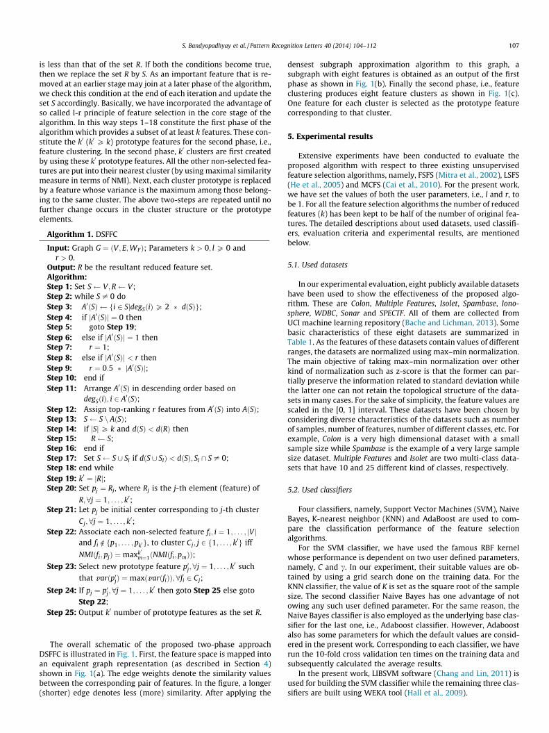
The overall schematic of the proposed two-phase approachDSFFC is illustrated in Fig. 1. First, the feature space is mapped intoan equivalent graph representation (as described in Section 4)shown in Fig. 1(a). The edge weights denote the similarity valuesbetween the corresponding pair of features. In the figure, a longer(shorter) edge denotes less (more) similarity. After applying the

densest subgraph approximation algorithm to this graph, asubgraph with eight features is obtained as an output of the firstphase as shown in Fig. 1(b). Finally the second phase, i.e., featureclustering produces eight feature clusters as shown in Fig. 1(c).One feature for each cluster is selected as the prototype featurecorresponding to that cluster.

5. Experimental results

Extensive experiments have been conducted to evaluate theproposed algorithm with respect to three existing unsupervisedfeature selection algorithms, namely, FSFS (Mitra et al., 2002), LSFS(He et al., 2005) and MCFS (Cai et al., 2010). For the present work,we have set the values of both the user parameters, i.e., l and r, tobe 1. For all the feature selection algorithms the number of reducedfeatures (k) has been kept to be half of the number of original fea-tures. The detailed descriptions about used datasets, used classifi-ers, evaluation criteria and experimental results, are mentionedbelow.

5.1. Used datasets

In our experimental evaluation, eight publicly available datasetshave been used to show the effectiveness of the proposed algo-rithm. These are Colon, Multiple Features, Isolet, Spambase, Iono-sphere, WDBC, Sonar and SPECTF. All of them are collected fromUCI machine learning repository (Bache and Lichman, 2013). Somebasic characteristics of these eight datasets are summarized inTable 1. As the features of these datasets contain values of differentranges, the datasets are normalized using max–min normalization.The main objective of taking max–min normalization over otherkind of normalization such as z-score is that the former can par-tially preserve the information related to standard deviation whilethe latter one can not retain the topological structure of the data-sets in many cases. For the sake of simplicity, the feature values arescaled in the [0, 1] interval. These datasets have been chosen byconsidering diverse characteristics of the datasets such as numberof samples, number of features, number of different classes, etc. Forexample, Colon is a very high dimensional dataset with a smallsample size while Spambase is the example of a very large samplesize dataset. Multiple Features and Isolet are two multi-class data-sets that have 10 and 25 different kind of classes, respectively.

5.2. Used classifiers

Four classifiers, namely, Support Vector Machines (SVM), NaiveBayes, K-nearest neighbor (KNN) and AdaBoost are used to com-pare the classification performance of the feature selectionalgorithms.

For the SVM classifier, we have used the famous RBF kernelwhose performance is dependent on two user defined parameters,namely, C and c. In our experiment, their suitable values are ob-tained by using a grid search done on the training data. For theKNN classifier, the value of K is set as the square root of the samplesize. The second classifier Naive Bayes has one advantage of notowing any such user defined parameter. For the same reason, theNaive Bayes classifier is also employed as the underlying base clas-sifier for the last one, i.e., Adaboost classifier. However, Adaboostalso has some parameters for which the default values are consid-ered in the present work. Corresponding to each classifier, we haverun the 10-fold cross validation ten times on the training data andsubsequently calculated the average results.

In the present work, LIBSVM software (Chang and Lin, 2011) isused for building the SVM classifier while the remaining three clas-sifiers are built using WEKA tool (Hall et al., 2009).

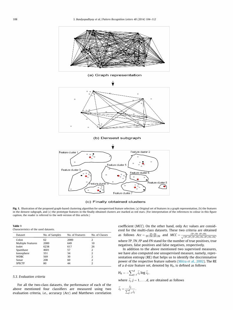
Fig. 1. Illustration of the proposed graph-based clustering algorithm for unsupervised feature selection. (a) Original set of features in a graph representation, (b) the featuresin the densest subgraph, and (c) the prototype features in the finally obtained clusters are marked as red stars. (For interpretation of the references to colour in this figurecaption, the reader is referred to the web version of this article.)

Table 1Characteristics of the used datasets.

Dataset No. of Samples No. of Features No. of Classes

Colon 62 2000 2Multiple Features 2000 649 10Isolet 6238 617 26Spambase 4601 57 2Ionosphere 351 34 2WDBC 569 30 2Sonar 208 60 2SPECTF 80 44 2

108 S. Bandyopadhyay et al. / Pattern Recognition Letters 40 (2014) 104–112

5.3. Evaluation criteria

For all the two-class datasets, the performance of each of theabove mentioned four classifiers are measured using twoevaluation criteria, i.e., accuracy (Acc) and Matthews correlation

coefficient (MCC). On the other hand, only Acc values are consid-ered for the multi-class datasets. These two criteria are obtainedas follows Acc ¼ TPþTN

TPþTNþFPþFN and MCC ¼ ðTP�TN�FP�FNÞffiffiffiffiffiffiffiffiffiffiffiffiffiffiffiffiffiffiffiffiffiffiffiffiffiffiffiffiffiffiffiffiffiffiffiffiffiffiffiffiffiffiffiffiffiffiffiffiffiðTPþFPÞðTPþFNÞðTNþFPÞðTNþFNÞp ,

where TP; TN; FP and FN stand for the number of true positives, truenegatives, false positives and false negatives, respectively.

In addition to the above mentioned two supervised measures,we have also computed one unsupervised measure, namely, repre-sentation entropy (RE) that helps us to identify the discriminativepower of the respective feature subsets (Mitra et al., 2002). The REof a d-size feature set, denoted by HR, is defined as follows

HR ¼ �Xd

j¼1ekj log ekj ;

where ekj ; j ¼ 1; . . . ;d, are obtained as follows

ekj ¼kjPdj¼1kj

:

S. Bandyopadhyay et al. / Pattern Recognition Letters 40 (2014) 104–112 109

Here, kj; j ¼ 1; . . . ;d, are the eigenvalues of the d� d covariance ma-trix of the respective feature space of size d.

The value of HR attains a maximum value when all the eigenvectors become equally important, i.e., the level of uncertainty ismaximum. On the other hand, its value equals to zero when allthe eigen values except one are zero. Higher value of RE indicatesbetter selection of features. RE is one of the most desired propertyto compare several feature selection algorithms.

5.4. Comparative study

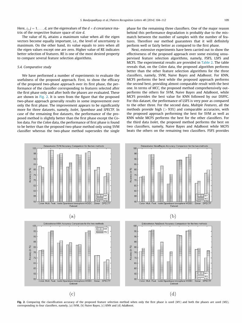
We have performed a number of experiments to evaluate theusefulness of the proposed approach. First, to show the efficacyof the proposed two-phase approach over its first phase, the per-formance of the classifier corresponding to features selected afterthe first phase only and after both the phases are evaluated. Theseare shown in Fig. 2. It is seen from the figure that the proposedtwo-phase approach generally results in some improvement overonly the first phase. The improvement appears to be significantlymore for three datasets, namely, Isolet, Spambase and SPECTF. Incase of the remaining five datasets, the performance of the pro-posed method is slightly better than the first phase except the Co-lon data. For the Colon data, the performance of first phase is foundto be better than the proposed two-phase method only using SVMclassifier whereas the two-phase method supersedes the single

Fig. 2. Comparing the classification accuracy of the proposed feature selection methcorresponding to four classifiers, namely, (a) SVM, (b) Naive Bayes, (c) KNN and (d) Ada

phase for the remaining three classifiers. One of the major reasonbehind this performance degradation is probably due to the mis-match between the number of samples with the number of fea-tures. Therefore our method guarantees that it will definitelyperform well or fairly better as compared to the first phase.

Next, extensive experiments have been carried out to show theeffectiveness of the proposed approach over some existing unsu-pervised feature selection algorithms, namely, FSFS, LSFS andMCFS. The experimental results are provided in Table 2. The tablereveals that, on the Colon data, the proposed algorithm performsbetter than the other feature selection algorithms for the threeclassifiers, namely, SVM, Naive Bayes and AdaBoost. For KNN,MCFS performs the best while the proposed approach performsthe second best, providing almost comparable result with the bestone. In terms of MCC, the proposed method comprehensively out-performs the others for SVM, Naive Bayes and AdaBoost, whileMCFS provides the best value for KNN followed by our DSFFC.For this dataset, the performance of LSFS is very poor as comparedto the other three. For the second data, Multiple Features, all themethods provide high (> 93%) and comparable accuracies, withthe proposed approach performing the best for SVM as well asKNN while MCFS performs the best for the other classifiers. Forthe third data Isolet, the proposed method performs the best ontwo classifiers, namely, Naive Bayes and AdaBoost while MCFSbeats the others on the remaining two classifiers. FSFS provides

od when only the first phase is used (M1) and both the phases are used (M2),Boost.

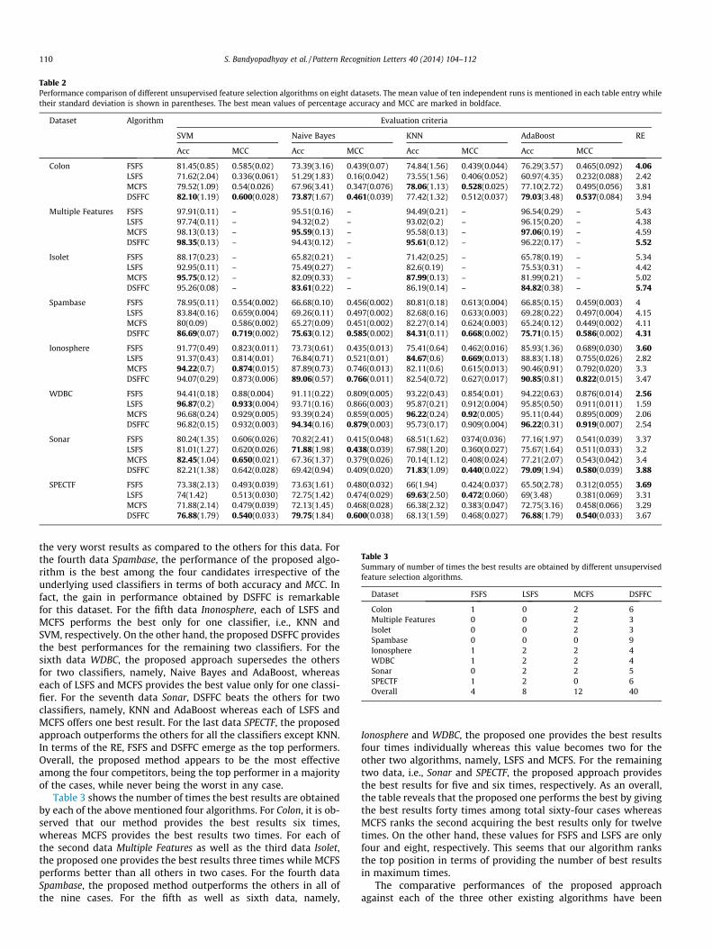
Table 3Summary of number of times the best results are obtained by different unsupervisedfeature selection algorithms.

Dataset FSFS LSFS MCFS DSFFC

Colon 1 0 2 6Multiple Features 0 0 2 3Isolet 0 0 2 3Spambase 0 0 0 9Ionosphere 1 2 2 4WDBC 1 2 2 4Sonar 0 2 2 5SPECTF 1 2 0 6Overall 4 8 12 40

Table 2Performance comparison of different unsupervised feature selection algorithms on eight datasets. The mean value of ten independent runs is mentioned in each table entry whiletheir standard deviation is shown in parentheses. The best mean values of percentage accuracy and MCC are marked in boldface.

Dataset Algorithm Evaluation criteria

SVM Naive Bayes KNN AdaBoost RE

Acc MCC Acc MCC Acc MCC Acc MCC

Colon FSFS 81.45(0.85) 0.585(0.02) 73.39(3.16) 0.439(0.07) 74.84(1.56) 0.439(0.044) 76.29(3.57) 0.465(0.092) 4.06LSFS 71.62(2.04) 0.336(0.061) 51.29(1.83) 0.16(0.042) 73.55(1.56) 0.406(0.052) 60.97(4.35) 0.232(0.088) 2.42MCFS 79.52(1.09) 0.54(0.026) 67.96(3.41) 0.347(0.076) 78.06(1.13) 0.528(0.025) 77.10(2.72) 0.495(0.056) 3.81DSFFC 82.10(1.19) 0.600(0.028) 73.87(1.67) 0.461(0.039) 77.42(1.32) 0.512(0.037) 79.03(3.48) 0.537(0.084) 3.94

Multiple Features FSFS 97.91(0.11) – 95.51(0.16) – 94.49(0.21) – 96.54(0.29) – 5.43LSFS 97.74(0.11) – 94.32(0.2) – 93.02(0.2) – 96.15(0.20) – 4.38MCFS 98.13(0.13) – 95.59(0.13) – 95.58(0.13) – 97.06(0.19) – 4.59DSFFC 98.35(0.13) – 94.43(0.12) – 95.61(0.12) – 96.22(0.17) – 5.52

Isolet FSFS 88.17(0.23) – 65.82(0.21) – 71.42(0.25) – 65.78(0.19) – 5.34LSFS 92.95(0.11) – 75.49(0.27) – 82.6(0.19) – 75.53(0.31) – 4.42MCFS 95.75(0.12) – 82.09(0.33) – 87.99(0.13) – 81.99(0.21) – 5.02DSFFC 95.26(0.08) – 83.61(0.22) – 86.19(0.14) – 84.82(0.38) – 5.74

Spambase FSFS 78.95(0.11) 0.554(0.002) 66.68(0.10) 0.456(0.002) 80.81(0.18) 0.613(0.004) 66.85(0.15) 0.459(0.003) 4LSFS 83.84(0.16) 0.659(0.004) 69.26(0.11) 0.497(0.002) 82.68(0.16) 0.633(0.003) 69.28(0.22) 0.497(0.004) 4.15MCFS 80(0.09) 0.586(0.002) 65.27(0.09) 0.451(0.002) 82.27(0.14) 0.624(0.003) 65.24(0.12) 0.449(0.002) 4.11DSFFC 86.69(0.07) 0.719(0.002) 75.63(0.12) 0.585(0.002) 84.31(0.11) 0.668(0.002) 75.71(0.15) 0.586(0.002) 4.31

Ionosphere FSFS 91.77(0.49) 0.823(0.011) 73.73(0.61) 0.435(0.013) 75.41(0.64) 0.462(0.016) 85.93(1.36) 0.689(0.030) 3.60LSFS 91.37(0.43) 0.814(0.01) 76.84(0.71) 0.521(0.01) 84.67(0.6) 0.669(0.013) 88.83(1.18) 0.755(0.026) 2.82MCFS 94.22(0.7) 0.874(0.015) 87.89(0.73) 0.746(0.013) 82.11(0.6) 0.615(0.013) 90.46(0.91) 0.792(0.020) 3.3DSFFC 94.07(0.29) 0.873(0.006) 89.06(0.57) 0.766(0.011) 82.54(0.72) 0.627(0.017) 90.85(0.81) 0.822(0.015) 3.47

WDBC FSFS 94.41(0.18) 0.88(0.004) 91.11(0.22) 0.809(0.005) 93.22(0.43) 0.854(0.01) 94.22(0.63) 0.876(0.014) 2.56LSFS 96.87(0.2) 0.933(0.004) 93.71(0.16) 0.866(0.003) 95.87(0.21) 0.912(0.004) 95.85(0.50) 0.911(0.011) 1.59MCFS 96.68(0.24) 0.929(0.005) 93.39(0.24) 0.859(0.005) 96.22(0.24) 0.92(0.005) 95.11(0.44) 0.895(0.009) 2.06DSFFC 96.82(0.15) 0.932(0.003) 94.34(0.16) 0.879(0.003) 95.73(0.17) 0.909(0.004) 96.22(0.31) 0.919(0.007) 2.54

Sonar FSFS 80.24(1.35) 0.606(0.026) 70.82(2.41) 0.415(0.048) 68.51(1.62) 0374(0.036) 77.16(1.97) 0.541(0.039) 3.37LSFS 81.01(1.27) 0.620(0.026) 71.88(1.98) 0.438(0.039) 67.98(1.20) 0.360(0.027) 75.67(1.64) 0.511(0.033) 3.2MCFS 82.45(1.04) 0.650(0.021) 67.36(1.37) 0.379(0.026) 70.14(1.12) 0.408(0.024) 77.21(2.07) 0.543(0.042) 3.4DSFFC 82.21(1.38) 0.642(0.028) 69.42(0.94) 0.409(0.020) 71.83(1.09) 0.440(0.022) 79.09(1.94) 0.580(0.039) 3.88

SPECTF FSFS 73.38(2.13) 0.493(0.039) 73.63(1.61) 0.480(0.032) 66(1.94) 0.424(0.037) 65.50(2.78) 0.312(0.055) 3.69LSFS 74(1.42) 0.513(0.030) 72.75(1.42) 0.474(0.029) 69.63(2.50) 0.472(0.060) 69(3.48) 0.381(0.069) 3.31MCFS 71.88(2.14) 0.479(0.039) 72.13(1.45) 0.468(0.028) 66.38(2.32) 0.383(0.047) 72.75(3.16) 0.458(0.066) 3.29DSFFC 76.88(1.79) 0.540(0.033) 79.75(1.84) 0.600(0.038) 68.13(1.59) 0.468(0.027) 76.88(1.79) 0.540(0.033) 3.67

110 S. Bandyopadhyay et al. / Pattern Recognition Letters 40 (2014) 104–112

the very worst results as compared to the others for this data. Forthe fourth data Spambase, the performance of the proposed algo-rithm is the best among the four candidates irrespective of theunderlying used classifiers in terms of both accuracy and MCC. Infact, the gain in performance obtained by DSFFC is remarkablefor this dataset. For the fifth data Inonosphere, each of LSFS andMCFS performs the best only for one classifier, i.e., KNN andSVM, respectively. On the other hand, the proposed DSFFC providesthe best performances for the remaining two classifiers. For thesixth data WDBC, the proposed approach supersedes the othersfor two classifiers, namely, Naive Bayes and AdaBoost, whereaseach of LSFS and MCFS provides the best value only for one classi-fier. For the seventh data Sonar, DSFFC beats the others for twoclassifiers, namely, KNN and AdaBoost whereas each of LSFS andMCFS offers one best result. For the last data SPECTF, the proposedapproach outperforms the others for all the classifiers except KNN.In terms of the RE, FSFS and DSFFC emerge as the top performers.Overall, the proposed method appears to be the most effectiveamong the four competitors, being the top performer in a majorityof the cases, while never being the worst in any case.

Table 3 shows the number of times the best results are obtainedby each of the above mentioned four algorithms. For Colon, it is ob-served that our method provides the best results six times,whereas MCFS provides the best results two times. For each ofthe second data Multiple Features as well as the third data Isolet,the proposed one provides the best results three times while MCFSperforms better than all others in two cases. For the fourth dataSpambase, the proposed method outperforms the others in all ofthe nine cases. For the fifth as well as sixth data, namely,

Ionosphere and WDBC, the proposed one provides the best resultsfour times individually whereas this value becomes two for theother two algorithms, namely, LSFS and MCFS. For the remainingtwo data, i.e., Sonar and SPECTF, the proposed approach providesthe best results for five and six times, respectively. As an overall,the table reveals that the proposed one performs the best by givingthe best results forty times among total sixty-four cases whereasMCFS ranks the second acquiring the best results only for twelvetimes. On the other hand, these values for FSFS and LSFS are onlyfour and eight, respectively. This seems that our algorithm ranksthe top position in terms of providing the number of best resultsin maximum times.

The comparative performances of the proposed approachagainst each of the three other existing algorithms have been

Table 4Summary of comparative performances of different unsupervised feature selection algorithms. The entry in the row X under the column W–D–L (Y) means win–draw–loss ofDSFFC compared to Y on the X dataset. The entry in the row X under the column SW–SL (Y) means significant win–significant loss of DSFFC compared to Y on the X dataset.

W–D–L (FSFS) SW–SL (FSFS) W–D–L (LSFS) SW–SL (LSFS) W–D–L (MCFS) SW–SL (MCFS)

Colon 8–0–1 2–0 9–0–0 8–0 7–0–2 4–0Multiple Features 3–0–2 2–2 5–0–0 2–0 3–0–2 1–2Isolet 5–0–0 4–0 5–0–0 4–0 3–0–2 2–2Spambase 9–0–0 8–0 9–0–0 8–0 9–0–0 8–0Ionosphere 8–0–1 8–0 7–0–2 6–2 7–0–2 2–0WDBC 8–0–1 8–0 5–0–4 2–0 7–0–2 4–2Sonar 7–0–2 2–0 7–0–2 4–1 7–0–2 2–0SPECTF 8–0–1 4–0 7–0–2 4–0 9–0–0 3–0Overall 56–0–8 38–2 54–0–10 38–3 52–0–12 26–6

S. Bandyopadhyay et al. / Pattern Recognition Letters 40 (2014) 104–112 111

summarized in Table 4. The table has mainly analyzed two criteria,namely, Win-Draw-Loss (W–D–L) and Significant Win-SignificantLoss (SW–SL) in which the value of SW–SL is computed usingone-way paired sample t-test. In the present analysis, thep-value = 0:01 is considered to be the threshold for showing thecorresponding result to be significant. For the first dataset Colon,the W–D–L of the proposed algorithm over FSFS, LSFS and MCFSare 8–0–1, 9–0–0 and 7–0–2, respectively. Also, the values ofSW–SL of DSFFC over the other three approaches are 2–0, 8–0and 4–0, respectively. These results indicate that the proposedone attains very good results as compared to the other three. Forthe second dataset Multiple Features, the W–D–L of the proposedtechnique over the other three are 3–0–2, 5–0–0 and 3–0–2,respectively and accordingly the values corresponding to SW–SLare 2–2, 2–0 and 1–2, respectively. These results indicate thatDSFFC performs better than LSFS and has almost similar perfor-mance against FSFS. This is the only dataset in which any other fea-ture selection algorithm (MCFS in this case) wins significantly themost number of times than it loses significantly in comparison toDSFFC. For the third dataset Isolet, DSFFC achieves better perfor-mance as compared to FSFS as well as LSFS whereas it performsequally well with respect to MCFS. For the fourth data Spambase,the W–D–L and SW–SL of the proposed technique over each ofthe remaining three algorithms are 9–0–0 and 8–0, respectively.These results signify that DSFFC achieves outstanding performancefor this data. For the fifth dataset Ionosphere, almost the sameobservation is found as compared to the remaining three methods.However, each of LSFS and MCFS provides two win values againstthe proposed approach in which the win of only LSFS is found to besignificant. For the sixth data WDBC, the proposed DSFFC performsremarkably well as compared to FSFS just like the fourth and fifthdatasets. Although the proposed technique beats LSFS in terms ofthe number of significant win, this is the only one case where LSFSperforms almost equally well as compared to DSFFC in terms of thenumber of win. For the seventh as well as eight data, i.e., Sonar andSPECTF, we observe that the proposed algorithm performs verywell as compared to each of the three competitors. These summaryinformation once again establish the superiority of the proposedapproach over the other existing unsupervised feature selectionalgorithms.

6. Conclusion

In this paper, a novel unsupervised feature selection algorithmhas been developed by integrating the concept of densest subgraphfinding with feature clustering. The proposed two-phase approachimproves classifier performance by selecting an optimal featuresubset that not only minimizes the mutual dependency amongthe chosen features but also maximizes the mutual dependencyof the selected features against the non-selected features. In thiswork, a novel existing normalized mutual information is also uti-lized to compute the similarity between two features.

Acknowledgements

Tapas Bhadra gratefully acknowledges Department of Scienceand Technology, India for awarding him the INSPIRE Fellowship(via. office order No. DST/INSPIRE Fellowship/2011/208) to carryout his Ph.D. research work. Sanghamitra Bandyopadhyay grate-fully acknowledges the financial support from the Swarnajayantiproject Grant No. DST/SJF/ET-02/2006-07 of the Department ofScience and Technology, Government of India.

References

Bache, K., Lichman, M., 2013. UCI machine learning repository. University ofCalifornia, Irvine, School of Information and Computer Sciences. <http://archive.ics.uci.edu/ml>.

Bahmani, B., Kumar, R., Vassilvitskii, S., 2012. Densest subgraph in streaming andmapreduce. In: Proceedings of VLDB Endowment, vol. 5, pp. 454–465.

Battiti, R., 1994. Using mutual information for selecting features in supervisedneural net learning. IEEE Trans. Neural Networks 5, 537–550.

Biesiada, J., Duch, W., 2008. Feature selection for high-dimensional data: a Pearsonredundancy based filter. Adv. Soft Comput. 45, 242–249.

Cai, D., Zhang, C., He, X., 2010. Unsupervised feature selection for multi-cluster data.In: Proceedings of the 16th ACM SIGKDD international conference onKnowledge discovery and data mining. Washington, USA, pp. 333–342.

Chang, C.C., Lin, C.J., 2011. LIBSVM: a library for support vector machines. ACMTrans. Intell. Syst. Technol. (TIST) 2, 27-1–27-27.

Cover, T.M., Thomas, J.A., 2012. Elements of Information Theory. John Wiley & Sons,New York, USA.

Dash, M., Liu, H., 1997. Feature selection for classification. Intell. Data Anal. 1, 131–156.

Estévez, P.A., Tesmer, M., Perez, C.A., Zurada, J.M., 2009. Normalized mutualinformation feature selection. IEEE Trans. Neural Networks 20, 189–201.

Hall, M., Frank, E., Holmes, G., Pfahringer, B., Reutemann, P., Witten, I., 2009. TheWEKA data mining software: an update. ACM SIGKDD Explor. Newslett. 11, 10–18.

He, X., Cai, D., Niyogi, P., 2005. Laplacian score for feature selection. In: Advances inNeural Information Processing Systems. MIT Press, pp. 507–514.

Hua, J., Tembe, W., Dougherty, E.R., 2008. Feature selection in the classification ofhigh-dimension data. In: IEEE International Workshop on Genomic SignalProcessing and Statistics, pp. 1–2.

Jin, X., Xu, A., Bie, R., Guo, P., 2006. Machine learning techniques and chi-squarefeature selection for cancer classification using SAGE gene expression profiles.Lecture Notes in Computer Science, vol. 3916, pp. 106–115.

Kohavi, R., John, G.H., 1997. Wrappers for feature subset selection. Art. Intell. 97,273–324.

Kononenko, I., 1994. Estimating attributes: analysis and extensions of RELIEF. In:Machine Learning: ECML-94, pp. 171–182.

Kwak, N., Choi, C., 2002. Input feature selection by mutual information based onparzen window. IEEE Trans. Pattern Anal. Mach. Intell. 24, 1667–1671.

Liao, C., Li, S., Luo, Z., 2007. Gene selection using Wilcoxon rank sum test andsupport vector machine for cancer classification. Lecture Notes in ComputerScience, vol. 4456, pp. 57–66.

Liu, S., Liu, H., Latecki, L.J., Yan, S., Xu, C., Lu, H., 2011. Size adaptive selection of mostinformative features. AAAI, 392–397.

Mandal, M., Mukhopadhyay, A., 2013. Unsupervised non-redundant featureselection: a graph-theoretic approach. In: Proceedings of the InternationalConference on Frontiers of Intelligent Computing: Theory and Applications(FICTA), pp. 373–380.

Mitra, P., Murthy, C.A., Pal, S.K., 2002. Unsupervised feature selection using featuresimilarity. IEEE Trans. Pattern Anal. Mach. Intell. 24, 301–312.

Peng, H., Long, F., Ding, C., 2005. Feature selection based on mutual information:criteria of max-dependency, max-relevance and min-redundancy. IEEE Trans.Pattern Anal. Mach. Intell. 27, 1226–1238.

112 S. Bandyopadhyay et al. / Pattern Recognition Letters 40 (2014) 104–112

Strehl, A., Ghosh, J., 2002. Cluster ensembles – a knowledge reuse framework forcombining multiple partitions. J. Mach. Learn. Res. 3, 583–617.

Vinh, L.T., Thang, N.D., Lee, Y.K., 2010. An improved maximum relevance andminimum redundancy feature selection algorithm based on normalized mutualinformation. In: 10th Annual International Symposium on Applications and theInternet, pp. 395–398.

Witten, I.H., Frank, E., 2005. Data Mining: Practical Machine Learning Tools andTechniques. Morgan Kaufmann, San Francisco, USA.

Yang, Y., Shen, H., Ma, Z., Huang, Z., Zhou, X., 2011. L2;1-norm regularizeddiscriminative feature selection for unsupervised learning. In: Proceedings ofthe Twenty-Second International Joint Conference on Artificial Intelligence,Barcelona, Spain, pp. 1589–1594.

Zhao, Z., Liu, H., 2007. Spectral feature selection for supervised and unsupervisedlearning. In: Proceedings of the 24th International Conference on MachineLearning, Corvallis, OR, pp. 1151–1157.