Pattern Recognition and Machine Learning · F-Measure The F-measures combine precision and recall into a single value. The F measures measure the effectiveness of retrieval with respect

Pattern Recognition and Machine Learning

James L. Crowley

ENSIMAG 3 - MMIS Fall Semester 2016 Lesson 2 12 October 2016

Face Detection using Color Histograms

Outline

Notation ...................................................................... 2

1. Two-Class Pattern Detectors................................... 3

2. Performance Evaluation Metrics............................. 5 ROC Curves ............................................................................... 5 True Positives and False Positives .............................................. 5 Precision and Recall ................................................................... 7 F-Measure .................................................................................. 7 Accuracy: ................................................................................... 8 Matthews Correlation Coefficient............................................... 8

3. Detecting Skin Pixels in Color histograms ........... 10 Histograms as an Estimation of Probability of Color ................ 12 Color Skin Detection using Luminance and Chrominance........ 12

4. Bayesian Tracking of Gaussian Blobs .................. 15 Moment Calculations for Blobs ................................................ 15 Bayesian Tracking (extra material)........................................... 18

Detecting Skin with Color Lesson 2

2-2

Notation xd A feature. An observed or measured value.

!

! X A vector of D features. D The number of dimensions for the vector

!

! y The true class for an observation

!

! X

!

{! X m}

!

{ym} Training samples for learning.

!

ym An annotation (or ground truth) function

!

R(! X m ) The Detection function or Recognition function

!

R(! X m )" P,N{ }

M The number of training samples. MT The number of training samples in the target class

!

h(! X ) A multidimensional histogram of

!

! X

Q The number of cells in a histogram


2-3

1. Two-Class Pattern Detectors A pattern detector is a classifier with K=2. Class k=1: The target pattern. Class k=2: Everything else. Pattern detectors are used in computer vision, for example to detect faces, road signs, publicity logos, or other patterns of interest. They are also used in signal communications, data mining and many other domains. The pattern detector is learned as a detection function

!

g! X ( ) followed by a decision

rule, d(). The detection function is learned from a set of training data composed of M sample observations

!

{! X m} where each sample observation is labeled with an indicator

variable

!

{ym} ym = P or Positive for examples of the target pattern (class 1) ym = N or Negative for all other examples (class 2) A ratio of histograms can provides a discriminant function as :

!

g(! X ) = p(C1 |

! X ) =

h1(! X )

h1(! X )+ h2 (

! X )

=h1(! X )

h(! X )

where

!

h1(! X ) is the histogram of training samples for the target class

and

!

h(! X ) is the histogram of ALL training samples.

To simplify the algebra, we can create a lookup table

!

L(! X ) =

h1(! X )

h(! X )

This gives a discriminant function of

!

g(! X ) = L(

! X )

Observations for which

!

g(! X ) > 0.5 are estimated to be members of the target class.

This will be called POSITIVE or P. Observations for which

!

g(! X ) " 0.5 are estimated to be members of the background.

This will be called NEGATIVE or N.


2-4

We can encode this as a decision function to define our detection function

!

R(! X m )

!

R(! X ) = d(g(

! X )) =

P if g(! X ) > 0.5

N if g(! X ) " 0.5

# $ %

For training we need ground truth (annotation). For each training sample the annotation or ground truth tells us the real class

!

ym

!

ym =P! X m " Target -Class

N otherwise

# $ %

The Classification can be TRUE or FALSE. if

!

R(! X m ) = ym then T else F

This gives

!

R(! X m ) = ym AND

!

R(! X m ) = P is a TRUE POSITIVE or TP

!

R(! X m ) " ym AND

!

R(! X m ) = P is a FALSE POSITIVE or FP

!

R(! X m ) " ym AND

!

R(! X m ) = N is a FALSE NEGATIVE or FN

!

R(! X m ) = ym AND

!

R(! X m ) = N is a TRUE NEGATIVE or TN

To better understand the detector we need a tool to explore the trade-off between making false detections (false positives) and missed detections (false negatives). The Receiver Operating Characteristic (ROC) provides such a tool


2-5

2. Performance Evaluation Metrics ROC Curves Two-class classifiers have long been used for signal detection problems in communications and have been used to demonstrate optimality for signal detection methods. The quality metric that is used is the Receiver Operating Characteristic (ROC) curve. This curve can be used to describe or compare any method for signal or pattern detection. The ROC curve is generated by adding a variable Bias term to a discriminant function.

!

R(! X ) = d(g(

! X )+ B)

and plotting the rate of true positive detection vs false positive detection where

!

R(! X m ) is the classifier as in lesson 1. As the bias term, B, is swept through a range of

values, it changes the ratio of true positive detection to false positives. For a ratio of histograms,

!

g(! X m ) is a probability ranging from 0 to 1.

B can range from less than –0.5 to more than +0.5. When B ≤ –0.5 all detections will be Negative. When B > +0.5 all detections will be Positive. Between –0.5 and +0.5

!

R(! X ) will give a mix of TP, TN, FP and FN.

The bias term, B, can act as an adjustable gain that sets the sensitivity of the detector. The bias term allows us to trade False Positives for False Negatives. The resulting curve is called a Receiver Operating Characteristics (ROC) curve. The ROC plots True Positive Rate (TPR) against False Positive Rate (FNR) as a function of B for the training data

!

{! X m} ,

!

{ym}.

True Positives and False Positives For each training sample, the detection as either Positive (P) or Negative (N) IF

!

g(! X m )+B > 0.5 THEN P else N

The detection can be TRUE (T) or FALSE (F) depending on the indicator variable ym IF

!

ym = R(! X m ) THEN T else F


2-6

Combining these two values, any detection can be a True Positive (TP), False Positive (FP), True Negative (TN) or False Negative (FN). For the M samples of the training data

!

{! X m} ,

!

{ym} we can define: #P as the number of Positives, #N as the number of Negatives, #T as the number of True and #F as the number of False, From this we can define: #TP as the number of True Positives, #FP as the number of False Positives, #TN as the number of True Negative, #FN as the number of False Negatives. Note that #P = #TP + #FN And #N = #FP+ #TN The True Positive Rate (TPR) is

!

TPR =#TP#P

=#TP

#TP+#FN

The False Positive Rate (FPR) is

!

FPR =#FP#N

=#FP

#FP+#TN

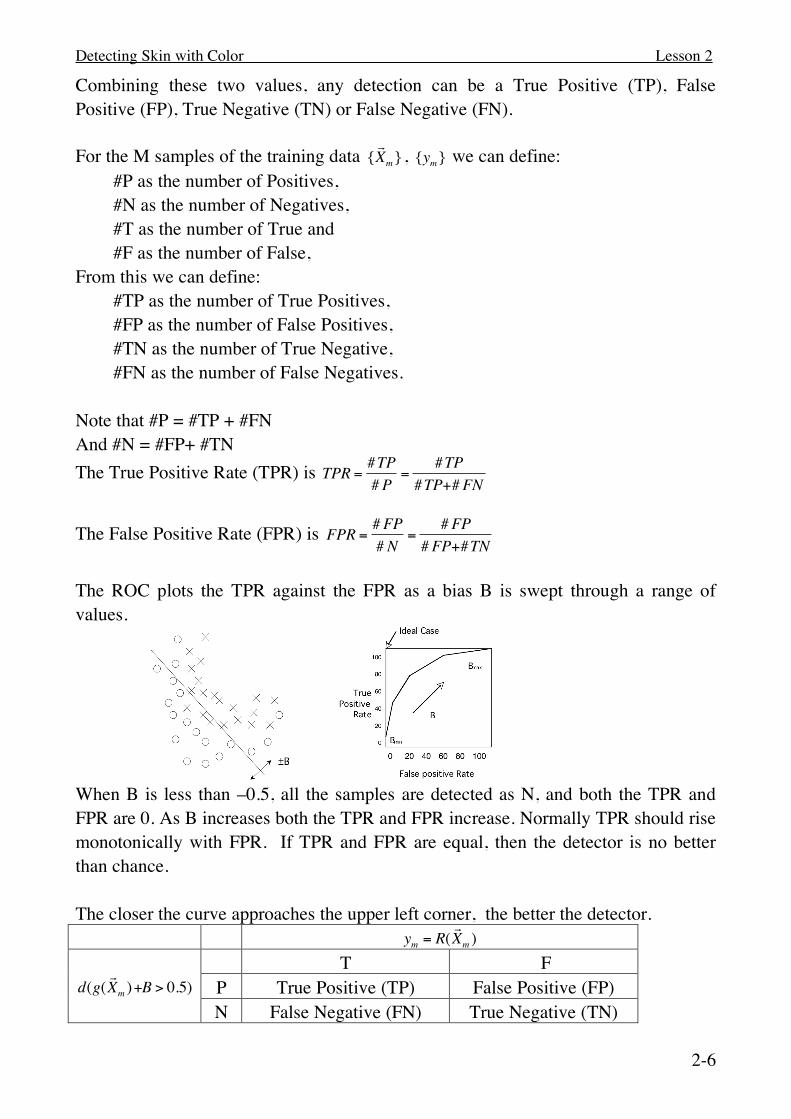
The ROC plots the TPR against the FPR as a bias B is swept through a range of values.

When B is less than –0.5, all the samples are detected as N, and both the TPR and FPR are 0. As B increases both the TPR and FPR increase. Normally TPR should rise monotonically with FPR. If TPR and FPR are equal, then the detector is no better than chance. The closer the curve approaches the upper left corner, the better the detector.

!

ym = R(! X m )

T F P True Positive (TP) False Positive (FP)

!

d(g(! X m )+B > 0.5)

N False Negative (FN) True Negative (TN)


2-7

Precision and Recall Precision, also called Positive Predictive Value(PPV) is the fraction of retrieved instances that are relevant to the problem.

!

PP =TP

TP+FP

A perfect precision score (PPV=1.0) means that every result retrieved by a search was relevant, but says nothing about whether all relevant documents were retrieved. Recall, also known as sensitivity (S), hit rate, and True Positive Rate (TPR) is the fraction of relevant instances that are retrieved.

!

S =TPR =TPT

=TP

TP+FN

A perfect recall score (TPR=1.0) means that all relevant documents were retrieved by the search, but says nothing about how many irrelevant documents were also retrieved. Both precision and recall are therefore based on an understanding and measure of relevance. In our case, “relevance” corresponds to “True”. Precision answers the question “How many of the Positive Elements are True ?” Recall answers the question “How many of the True elements are Positive”? In many domains, there is an inverse relationship between precision and recall. It is possible to increase one at the cost of reducing the other.

F-Measure The F-measures combine precision and recall into a single value. The F measures measure the effectiveness of retrieval with respect to a user who attaches 2 times as much importance to recall as precision. The F1 score weights recall higher than precision. F1 Score:


2-8

!

F1 =2TP

2TP+FP+FN

The F1 score is the harmonic mean of precision and sensitivity. This is the geometric mean divided by the arithmetic mean.

Accuracy: Accuracy is the fraction of test cases that are correctly classified (T).

!

ACC =TM

=TP+TNM

where M is the quantity of test data. Note that the terms Accuracy and Precision have a very different meaning in Measurement theory. In measurement theory, accuracy is the average distance from a true value, while precision is a measure of the reproducibility for the measurement.

Matthews Correlation Coefficient The Matthews correlation coefficient is a measure of the quality of binary (two-class) classifications. This measure was proposed by the biochemist Brian W. Matthews in 1975. MCC takes into account true and false positives and negatives and is generally regarded as a balanced measure that can be used even if the classes are of very different sizes. The MCC is in essence a correlation coefficient between the observed and predicted binary classifications MCC results a value between +1 and -1, where +1 represents a perfect prediction, 0 no better than random prediction and −1 indicates total disagreement between prediction and observation.

!

MCC =TP "TN #FP "FN

(TP+FP)(TP +FN )(TN +FP)(TN +FN )

The original formula given by matthews was:


2-9

M = Total quanitity of test data:

!

M =TN +TP+FN +FP

!

S =TP+FN

M

!

P =TP+FPM

!

MCC =TP

M " S #PPS(1" S)(1"P)


2-10

3. Detecting Skin Pixels in Color histograms A ratio of color histograms can be used to construct a simple detector for skin pixels in images. Color skin pixels can be used to detect faces, hands and other skin colored regions in images. Consider the images in the FDDB (Face Detection Data Set and Benchmark) data base maintained at UMASS: http://vis-www.cs.umass.edu/fddb/ This data-base was constructed for face detection and not for skin detection. Face regions have been hand-labeled as both boxes and ellipses. All images are RGB with each pixel containing 3 colors: Red, Green and Blue. We will use the ellipses as ground truth for skin regions. This will create errors in the training data. A typical image with and annotated face regions as an ellipse looks like:

Note that there are skin pixels that are NOT in the ellipse (hand, ears, neck etc), and there are non-skin pixels that ARE in the face (hair, teeth, etc). This will lead to minor errors in the detection. Your job will be to measure the impact of these errors in building a face detector using detection of skin pixels. Annotations of face regions are represented as an elliptical region, denoted by a 6-tuple (ra, rb, θ, cx, cy, 1) where ra and rb refer to the half-length of the major and minor axes, θ is the angle of the major axis with the horizontal axis, and cx and cy are the column and row image coordinates of the center of this ellipse. Ellipse Data: 2002/07/24/big/img_82 1 59.268600 35.142400 1.502079 149.366900 59.365500 1


2-11

the standard form of an ellipse with a major axis along the horizontal (x) axis is:

!

x " cx( )2

ra2 +

y" cy( )2

rb2 =1

when rotated by θ:

!

(x " cx )cos(#)+ (y" cy )sin(#)( )2

ra2 +

(x " cx )sin(#)+ (y" cy )cos(#)( )2

rb2 =1


2-12

Histograms as an Estimation of Probability of Color Assume that we have a color image, where each pixel (i,j) is a color vector,

!

! p (i, j), composed of 3 integers between 0 and 255 representing Red, Green and Blue.

!

! p (i, j) =

RGB

"

#

$ $ $

%

&

' ' '

We can build a color histogram of the image by counting the number of times that each unique value of (R, G, B) occurs in the image. To do this we allocate a table h(R, G, B) of 256 x 256 x 256 cells, with each cell initially set to zero. If each color is represented by 8 bits, then the table h(R, G, B) has Q=(28)3 cells. Q=(28)3=2563 = 224 = 24 · 220 = 16 Meg Cells. Using our rule of 8 samples per cell, we need 23x24 = 27 = 128 Meg Pixels. If the training data is composed of 128x128 images, then how many images do we need for h(X)? 128 x 128 pixels = 27 x 27 = 214 = 16 K pixels. Thus we need 8000 images ! What can we do? Often we can reduce both the number, D, of features and the number of values, N, for each feature. For example, for many color images, N=32 color values are sufficient to detect objects. We simply divide each color R, G, B by 8. R' = Trunc(R/8), G'=Trunc(G/8), B'=Trunc(B/8). This reduces our histogram to 8x8x8=(23)3 = 29=512 cells We can also use our knowledge of physics to look for features that are "invariant". Color Skin Detection using Luminance and Chrominance.

Luminance captures surface orientation (3D shape) while Chrominance is a signature for object pigment (identity). Thus it is convenient to transform the (RGB) color pixels into a color space that separates Luminance from Chrominance.


2-13

!

LC1C2

"

#

$ $ $

%

&

' ' ' (

RGB

"

#

$ $ $

%

&

' ' '

Normalizing out luminance provides a popular space for skin detection: the (r,g) space. Luminance: L= R+G+B Chrominance :

!

r = c1 =R

R+G + B

!

g = c2 =G

R+G + B

These are often called "r" and "g" in the literature. The (r, g) space is often used to detect skin colored pixels. It is common to normalize r and g to natural numbers coded with N values between 0 and N – 1 by :

!

r = trunc N " RR+G + B

#

$ %

&

' (

!

g = trunc N " GR+G + B

#

$ %

&

' (

Skin pigment is generally always the same chrominance value. Luminance can change with pigment density, and skin surface orientation, but chrominance will remain invariant. Thus we can use (r,g) as an invariant color signature for detecting skin in at each pixel. From experience, N = 32 color values seems to work well for skin, but larger values of N may work better with some data sets. Suppose we have a set of K training images {

!

! p (i, j)} of size RxC where each pixel is an RGB color vector. This gives a total of M=NxRxC color pixels. Suppose that MT of these are labeled as skin pixels. We allocate two table : h(r,g) and hskin(r,g) of size N x N. For all i,j,k in the training set

!

! p k (i, j){ } BEGIN

!


#

$ %

&

' (

!

g = trunc N " GR+G + B

#

$ %

&

' (

!

h(r,g) = h(r,g)+1 IF the pixel

!

! p k (i, j) is ∈ skin region THEN

!

hskin(r,g) = hskin(r,g)+1 and Mskin =Mskin+1 END


2-14

As before, we can obtain a lookup table Lskin(r,g) that gives the probability that a pixel is skin.

!

Lskin(r,g) =hskin(r,g)h(r,g)

Given a new RGB image

!

! p (i, j) for each pixel (i,j)

!


#

$ %

&

' (

!

g = trunc N "G

R +G + B#

$ %

&

' (

g(

!

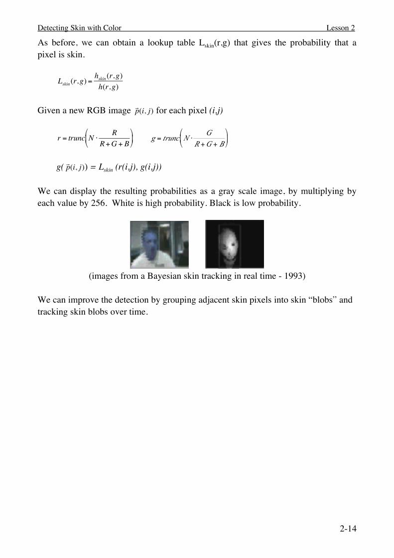
! p (i, j)) = Lskin (r(i,j), g(i,j)) We can display the resulting probabilities as a gray scale image, by multiplying by each value by 256. White is high probability. Black is low probability.

(images from a Bayesian skin tracking in real time - 1993)

We can improve the detection by grouping adjacent skin pixels into skin “blobs” and tracking skin blobs over time.


2-15

4. Bayesian Tracking of Gaussian Blobs Rather than represent a skin region as a collection of pixels, we can calculate a Gaussian Blob. A "Blob" represents a region of an image. Gaussian blobs express a region in terms of moments. Assume of image of probabilities of the detection of a target: T(i,j), where for each pixel: T(i,j) = Lskin(r(i,j), g(i,j)) The zeroth moment of the probabilities is the mass (sum of probabilities). Average mass represents confidence. The first moment gives is the center of gravity. This is the "position" of the blob. The second moment is the covariance. This gives size and orientation. We typically enclose the blob in some rectangular Region of Interest (ROI) in order to avoid "distraction" by neighboring blobs. The ROI is obtained by some form of estimation or a priori knowledge. In continuous operation the ROI be provided by tracking. Let us represent the ROI as a rectangle : (t,l,b,r) t - "top" - first row of the ROI. l - "left" - first column of the ROI. b - "bottom" - last row of the ROI r - "right" -last column of the ROI. (t,l,b,r) can be seen as a bounding box, expressed by opposite corners (l,t), (r,b) We will compute the moments within this ROI (bounding box). Moment Calculations for Blobs Given a target probability image T(i,j) and a ROI (t,l,b,r):

Sum:

!

S =i=l

r

" Tj=t

b

" (i, j)


2-16

We can estimate the "confidence" as the average detection probability: Confidence:

!

CF =S

(b " t)(r " l)

First moments:

!

x = µi =1S i=l

r

" Tj=t

b

" (i, j) # i

!

y = µ j =1S i=l

r

" Tj=t

b

" (i, j) # j

Position is the center of gravity: (µi, µj) We will use this as the position of the blob. Second Moments:

!

" i2 =1S i=l

r

# Tj=t

b

# (i, j) $ (i %µi )2

!

" j2 =1S i=l

r

# T (i, j) $ ( j %µ j )2

j=t

b

#

!

" ij2 =1S i=l

r

# Tj=t

b

# (i, j) $ (i %µi ) $ ( j %µ j )

These compose a covariance matrix:

!

C =" i2 " ij

2

" ij2 " j

2

#

$ %

&

' (

The principle components (λ1, λ2) determine the length and width. The principle direction determines the orientation of the length. We can discover these by principle components analysis.

!

RCRT =" =#12 00 #2

2

$

% &

'

( )

where

!

R =cos(" ) #sin(" )sin(" ) cos(" )$

% &

'

( )


2-17

The length to width ratio, λ1/λ2, is an invariant for shape. The angle θ is a “Covariant” for orientation. We can use the “eigenvalues”, or characteristic values, λ1, λ2, to define the “width and height” of the blob: For example: w=λ1, h=λ2

This suggests a "feature vector" for the blob:

!

! X =

xywh"

#

$

% % % % % %

&

'

( ( ( ( ( (

where x= µi, y = µj, w=λ1, h=λ2 and CF = S(b ! t)(r ! l)

The confidence (CF) can be seen as the “Likelihood” that the model for the blob is correct. Tracking allows us to continually update an estimate for the features of the Blob, even if the blob is temporarily lost to occlusion or noise. The tracked object is often referred to as a "target". The vector provides the “model” for the target blob:

Blob model:

!

! X =

xywh"

#

$

% % % % % %

&

'

( ( ( ( ( (

along with CF. (Confidence)

The precision of the blob can be represented by a covariance matrix

!

P =

" xx2 " xy

2 " xw2 " xh

2 " x#2

" yx2 " yy

2 " yw2 " yh

2 " y#2

" wx2 " wy

2 " ww2 " wh

2 " w#2

" hx2 " hy

2 " hw2 " hh

2 " h#2

"#x2 "#y

2 "#w2 "#h

2 "##2

$

%

& & & & & &

'

(

) ) ) ) ) )


2-18

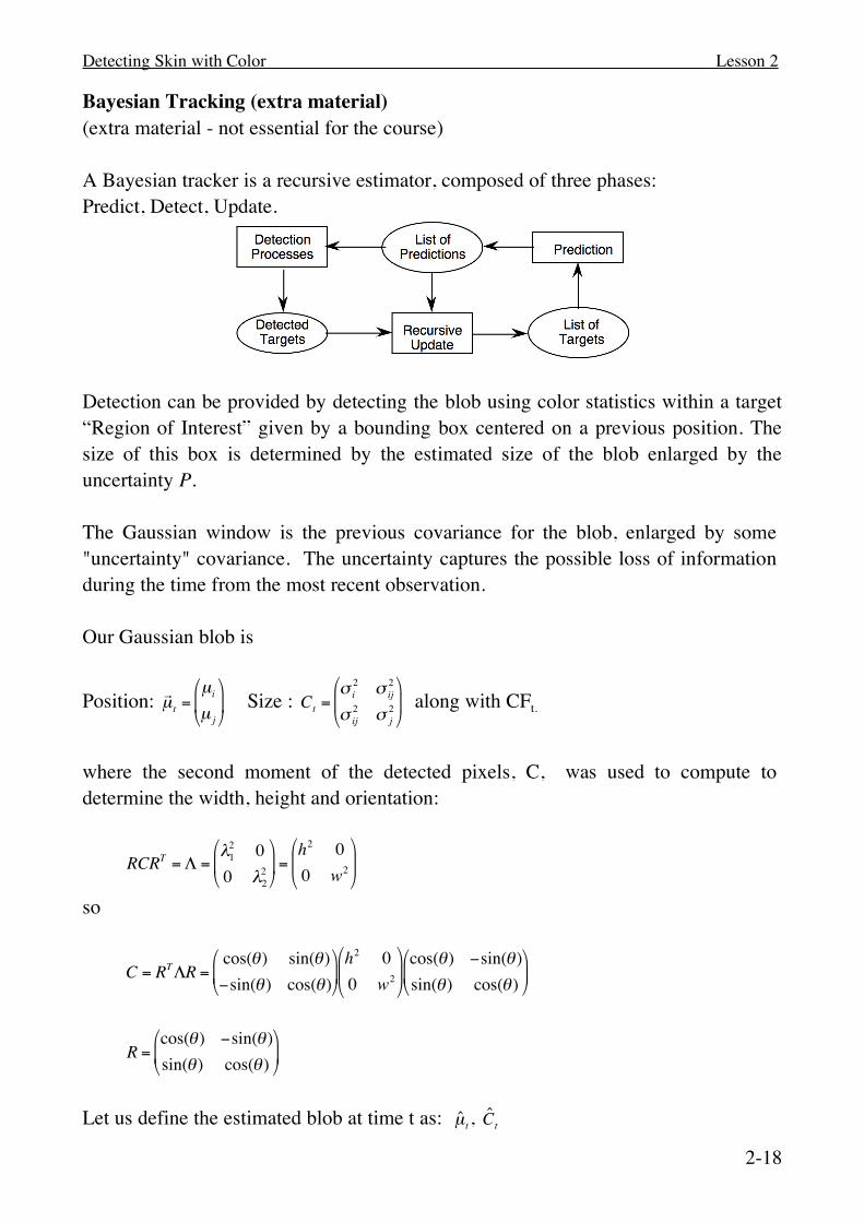
Bayesian Tracking (extra material) (extra material - not essential for the course) A Bayesian tracker is a recursive estimator, composed of three phases: Predict, Detect, Update.

Detection can be provided by detecting the blob using color statistics within a target “Region of Interest” given by a bounding box centered on a previous position. The size of this box is determined by the estimated size of the blob enlarged by the uncertainty P. The Gaussian window is the previous covariance for the blob, enlarged by some "uncertainty" covariance. The uncertainty captures the possible loss of information during the time from the most recent observation. Our Gaussian blob is

Position:

!

! µ t =

µi

µ j

"

# $

%

& ' Size :

!

Ct =" i2 " ij

2

" ij2 " j

2

#

$ %

&

' ( along with CFt.

where the second moment of the detected pixels, C, was used to compute to determine the width, height and orientation:

!

RCRT =" =#12 00 #2

2

$

% &

'

( ) =

h2 00 w2

$

% &

'

( )

so

!

C = RT"R =cos(# ) sin(#)$sin(# ) cos(#)%

& '

(

) * h2 00 w2

%

& '

(

) * cos(#) $sin(# )sin(#) cos(# )%

& '

(

) *

!

R =cos(" ) #sin(" )sin(" ) cos(" )$

% &

'

( )

Let us define the estimated blob at time t as:

!

ˆ µ t ,

!

ˆ C t


2-19

Let us define the predicted feature vector at time t as:

!

! µ t*,

!

Ct*

We will compute the estimated blob from by multiplying the detected pixels by a Gaussian mask determined from the predicted blob. The Covariance is multiplied by 2 to offset the fact that we will use mask to estimate a new covariance. Gaussian Mask:

!

G( ! µ t*,2Ct

* ) Detected target pixels:

!

t(i, j)" L(! c (i, j)) # e$12

ij%

& ' (

) * $

µi

µi

%

& '

(

) *

%

& '

(

) *

T

2Ct*–1 i

j%

& ' (

) * $

µi

µi

%

& '

(

) *

%

& '

(

) *

where L() is our lookup table for the ratio of histograms. This is a form of “robust” estimation that uses the Gaussian mask to reject “outlying” detections. We then estimate the new position and covariance as before:

First moments:

!

µi =1S i=l

r

" tj=t

b

" (i, j) # i

!

µ j =1S i=l

r

" tj=t

b

" (i, j) # j

Second Moments:

!

" i2 =1S i=l

r

# tj=t

b

# (i, j) $ (i %µi )2

!

" j2 =1S i=l

r

# tj=t

b

# (i, j) $ ( j %µ j )2

!

" ij2 =1S i=l

r

# tj=t

b

# (i, j) $ (i %µi ) $ ( j %µ j )

Position:

!

! ˆ µ t =µi

µ j

"

# $

%

& ' Size :

!

ˆ C t =" i

2 " ij2

" ij2 " j

2

#

$ %

&

' (

For this we must predict the new position, detect (observe) the blob, and the update the estimate. The following is a “zero-th” order Kalman filter. This is the simplest (almost trivial) case of a Bayesian tracker. A first order Kalman filters estimates parameters and their derivatives. The math is more complex but the principles are the same.

Documents

Pattern Recognition and Machine Learning · F-Measure The F-measures combine precision and recall into a single value. The F measures measure the effectiveness of retrieval with respect