Embed Size (px)
Citation preview

PATHOGEN DETECTION LAB-ON-A-CHIP (PADLOC) SYSTEM FOR PLANT
PATHOGEN DIAGNOSIS
A Thesis
by
OSMAN SAFA CIFCI
Submitted to the Office of Graduate Studies of
Texas A&M University
in partial fulfillment of the requirements for the degree of
MASTER OF SCIENCE
August 2012
Major Subject: Electrical Engineering

Pathogen Detection Lab-on-a-Chip (PADLOC) System for Plant Pathogen Diagnosis
Copyright 2012 Osman Safa Cifci

PATHOGEN DETECTION LAB-ON-A-CHIP (PADLOC) SYSTEM FOR PLANT
PATHOGEN DIAGNOSIS
A Thesis
by
OSMAN SAFA CIFCI
Submitted to the Office of Graduate Studies of
Texas A&M University
in partial fulfillment of the requirements for the degree of
MASTER OF SCIENCE
Approved by:
Chair of Committee, Arum Han
Committee Members, Xing Cheng
Jim Ji
Won-Bo Shim
Head of Department, Costas N. Georghiades
August 2012
Major Subject: Electrical Engineering

` iii
ABSTRACT
Pathogen Detection Lab-On-A-Chip (PADLOC) System for Plant Pathogen Diagnosis.
(August 2012)
Osman Safa Cifci, B.S., Eskisehir Osmangazi Univertsity
Chair of Advisory Committee: Dr. Arum Han
Polymerase Chain Reaction (PCR) detection paves the way to reliable and rapid
diagnosis of diseases and has been used extensively since its introduction. Many
miniaturized PCR systems were presented by microfluidics and lab-on-a-chip
community. However, most of the developed systems did not employ real-time
detection and thus required post-PCR processes to obtain results. Among the few real-
time PCR systems, almost all of them aimed for medical applications and those for plant
pathogen diagnosis systems are almost non-existent in the literature.
In this work, we are presenting a portable system that employs microfluidics
PCR system with integrated optical systems to accomplish real-time quantitative PCR
for plant pathogen diagnosis. The system is comprised of a PCR chip that has a chamber
for PCR sample with integrated metal heaters fabricated by standard microfabrication
procedures, an optical system that includes lenses, filters, a dichroic mirror and a
photomultiplier tube (PMT) to achieve sensitive fluorescence measurement capability
and a computer control system for Proportional Integral Derivative (PID) control and
data acquisition. The optical detection system employs portable components and has a
size of 3.9 x 5.9 x 11.9 cm which makes it possible to be used in field settings. On the

` iv
device side, two different designs are used. The first design includes a single chamber in
a 25.4 x 25.4 mm device and the capacity of the chamber is 9 µl which is sufficient to do
gel electrophoresis verification. The second design has three 2.2 µl chambers squeezed
in the same size device while having smaller volume to increase high throughput of the
system.
The operation of the system was demonstrated using Fusarium oxysporum spf.
lycopersici which is a fungal plant pathogen that affects crops in the USA. In the
presence of the plant pathogen, noticeable increases in the photomultiplier tube output
were observed which means successful amplifications and detections occurred. The
results were confirmed using gel electrophoresis which is a conventional post-PCR
process to determine the existence and length of the amplified DNA. Clear bands
located in the expected position were observed following the gel electrophoresis.
Overall, we have presented a portable PCR system that has the capability of
detecting plant pathogens.

` v
DEDICATION
To my dear family and friends for your unconditional love and support

` vi
ACKNOWLEDGEMENTS
I would like to thank my advisor and committee chair, Dr. Arum Han, for his
unwavering guidance and support all the way. I would like to thank my committee
members, Dr. Xing Cheng, Dr. Jim Ji, and Dr. Won-Bo Shim as well as Dr. Jun Zou for
their advice and support. My special thanks go to Dr. Shim for kindly providing me with
the opportunity to work in his lab.
I would like to thank my collaborator, Martha, for her patient tutorials and
generous help. I also want to thank my group members, Jaewon Park, Hyunsoo Kim,
Chiwan Koo, Han Wang, Celal Erbay, Haron Abdel-Raziq and Adrian Guzman, and
alumni Huijie Hou, Whitney Parker, and Jianzhang Wu for their enormous help in the
lab and in life. I would especially like to state my appreciation to Chiwan and Hyun Soo
for their involvement in the PADLOC project.
Life without Celal Erbay, Haron Abdel-Raziq and my roommate Ahmad
Bashaireh in College Station would definitely be an unpleasant experience. Thank you
all for offering your kind friendship.

` vii
TABLE OF CONTENTS
Page
ABSTRACT ..................................................................................................................... iii
DEDICATION ................................................................................................................... v
ACKNOWLEDGEMENTS .............................................................................................. vi
TABLE OF CONTENTS .................................................................................................vii
LIST OF FIGURES ........................................................................................................... ix
LIST OF TABLES ...........................................................................................................xii
CHAPTER I INTRODUCTION ........................................................................................ 1
1.1. Objective and Motivation for Plant Pathogen Detection ................................... 1 1.2. Conventional PCR Systems ............................................................................... 2 1.3. Microchip PCR Systems .................................................................................... 4
CHAPTER II MICROCHIP PCR SYSTEM ................................................................... 15
2.1 Design and Simulation of Heaters .................................................................... 15 2.2 Microfabrication of Devices............................................................................. 17 2.3 Temperature Characterization of Heaters ........................................................ 19 2.4 Optical System Design and Characterization ................................................... 23 2.5 Developments towards a Multi Chamber Microchip PCR Design .................. 30
CHAPTER III DEVELOPMENT OF THE PORTABLE PATHOGEN DETECTION
LAB ON A CHIP (PADLOC) ......................................................................................... 38
3.1 Overview of the PADLOC System .................................................................. 38 3.2 System Control and Operation ......................................................................... 39 3.3 Specifications of the System ............................................................................ 42
3.4 Sample and Reagents ....................................................................................... 43 3.5 Detection of Pure Genomic DNA .................................................................... 44 3.6 Multichamber Design Results .......................................................................... 47
CHAPTER IV SUMMARY AND FUTURE WORK ..................................................... 49
4.1 Project Review ................................................................................................. 49

` viii
Page
4.2 Future Work ..................................................................................................... 50
REFERENCES ................................................................................................................. 52
APPENDIX A COMSOL JOULE HEATING MANUAL ............................................. 60
APPENDIX B LABVIEW PROGRAM ......................................................................... 70
APPENDIX C MASK DESIGNS FOR HEATERS AND CHAMBERS ....................... 71
APPENDIX D MICROFABRICATION PROCEDURES ............................................. 75
VITA ................................................................................................................................ 78

` ix
LIST OF FIGURES
Page
Fig. 2.1 Top view (A) and cross-section (B) of the square spiral design………………16
Fig. 2.2 A picture of a PCR microchip having a chamber and heater bonded with a
UV glue………………………………………………………………………….18
Fig. 2.3 Microfabrication procedures…………………………………………………...19
Fig. 2.4 General working principle of PID control. The feedback is sent back to the
system for reliable control………………………………………………………20
Fig. 2.5 Schematic used to determine temperature settings. Two thermocouples
placed on different sides of the device………………………………………….21
Fig. 2.6 The temperature profile from the two thermocouples placed on different
sides of the device……………………………………………………………….22
Fig. 2.7 Full run of PCR cycle demonstrating repeatable temperature profile in each
cycle……………………………………………………………………………..23
Fig. 2.8 The optical housing schematic used in fluorescence measurement. The
blue ray is the trajectory of the LED and the green ray is the trajectory of
the fluorescent light coming from the sample……………………..…………...25
Fig. 2.9 Manufactured optical housing using 3D printer. The LED is placed inside
the housing and green septa rubbers are used to seal the inlet and outlet of
the microdevice…………………………………………………………………26
Fig. 2.10 Spectrophotometer results showing suitable excitation and emission
optical components. The excitation filter blocks out the green light coming
from the LED and only green light range is observed from the output……........28
Fig. 2.11 PMT characterization using fluorescent dye and PCR samples. Linear
increase in PMT output was observed for different dye concentrations.
Additionally, unamplified and amplified sample resulted in different PMT
outputs making it suitable for PCR experiments………………………………..30

` x
Page
Fig. 2.12 Simulation result of 4-bar design. Similar profile was observed from
middle chambers and edge chambers but the two groups have different
temperature profile………………………………………………………………32
Fig. 2.13 Simulation of one chamber in 4-bar design. The temperature difference
within the chamber is up to 5 degrees…………………………………………..33
Fig. 2.14 Temperature profile of the 4-bar design. The difference between two
thermocouples is significant and since the reference thermocouple is very
sensitive to location there is a run to run variance in this experiment…………..34
Fig. 2.15 Temperature simulations of serpentine design. Top views of (A) middle
and (B) edge chamber are shown. The temperature inside the chamber is
within 2 degrees…………………………………………………………………35
Fig. 2.16 Fabricated serpentine design microdevice…………………………………...36
Fig. 2.17 Temperature profile of the serpentine design. There is a small difference
between two thermocouples and the variance from run to run is small………...37
Fig. 3.1 Overall view of PADLOC system having microdevice, optical setup and
control and acquisition modules………………………………………………...38
Fig. 3.2 The structure of the Labview program for PCR experiments. It can be
regarded as a combination of two programs: One for temperature control
and one for data acquisition and display………………………………………...39
Fig. 3.3 Front-end of the Labview program. It allows entering temperature
durations and files to log the data as well as displays temperature and PMT
output data............................................................................................................41
Fig. 3.4 PMT outputs of three PCR runs. The fluorescence intensity increases were
shown...………………………………………………………………………….44

` xi
Page
Fig. 3.5 Gel electrophoresis results of PCR runs. The bands are observed between
200 and 300 bp. The first well is filled with DNA ladder to aid in
visualization of the bands……………………………………………………….46
Fig. 3.6 The PMT output graphs of serpentine design. The increases in signal
intensity are shown……………………………………………………………...48
Fig. A.1 Finalized Drawing of Heater………………………………………………….63
Fig. A.2 Finalized Drawing of Microdevice…………………………………….……...65
Fig. A.3 Application of Heat Flux….…………………………………………………..66
Fig. A.4 Structure of the Device After Meshing……………………………………….67
Fig. A.5 3D Overview of Simulation…………………………………………………...68
Fig. A.6 Cross-section View of the Chamber…………………………………………..69
Fig. B.1 Labview program used in PADLOC project………………………………….70
Fig. C.1 Big chamber design…………………………………………………………...71
Fig. C.2 Big heater design……………………………………………………………...72
Fig. C.3 Serpentine design chamber……………………………………………………73
Fig. C.4 Serpentine design heater design……………………………………………….74

` xii
LIST OF TABLES
Page
Table 3.1: PADLOC system and thermocycler temperature durations ............................ 43

` 1
CHAPTER I
INTRODUCTION
1.1. Objective and Motivation for Plant Pathogen Detection
Plant diseases result in billions of dollars loss every year to agriculture, landscape
and forestry in the United States.1 The reasons for economic losses are reduction in the
quality of the products, yield, aesthetic and nutritional value as well as contamination of
food via toxic means. Additionally, proper maintaining the land paves the way to
keeping and even increasing the food supplies while increasing the cultivated land
minimally. By managing the land, it is possible to protect the domestic crops against
foreign diseases and increase the export market for plant products. There is a need for
rapid and accurate detection of plant pathogen in order to avoid big economic losses in
crops. The control of a plant disease involves identifying the disease or finding the
pathogen causing the disease. There are many known pathogens and diseases by
scientist and the number of these increases by the introduction of emerging diseases
caused by previously unknown pathogen or mutation of known pathogens.
Previously, the pathogens used to be detected by in-vitro screens, microscopic
examination and biochemical tests. These methods take long time, require a specialist or
expensive materials. Therefore; new, sensitive, accurate, portable and inexpensive
methods are required for plant pathogen detection. The DNA based detection methods
are on the rise and are expected to be used to identify more and more pathogens. One of
____________
This thesis follows the style of Lab Chip.

` 2
the most commonly used DNA based diagnosis method is polymerase chain reaction
(PCR).2 As PCR becomes more and more common in the laboratory settings, the lab-
on-a-chip community presents more and more PCR systems that employ unique
properties of miniaturized systems. There are many miniaturized PCR systems
developed in the literature. However, most of the PCR work did not employ real-time
detection of PCR product and relied on post-PCR procedures. Out of the real-time PCR
systems were intended for medical field and real-time PCR detection for plant diseases
are almost non-existent in the literature. The motivation for this study is the
development of a portable plant pathogen detection system that employs polymerase
chain reaction to amplify target pathogens and at the same time detect the presence or
absence of the target pathogen that could be used in a field setting.
1.2. Conventional PCR Systems
The polymerase chain reaction (PCR) is a very useful laboratory tool that
selectively replicates DNA and is used in crop pathogen detection, clinical medicine,
genetic disease identification, forensics science among others. Since its introduction to
scientific literature,2 the method of amplifying a specific sequence has attracted much
attention. The very first PCR experiments used to be very laborious because of the
requirement of fresh enzyme addition during the run. However, this did not take long
and PCR protocol was automated with the introduction of DNA polymerase obtained by
thermophiles by Lawyer.3 This was the breakthrough that renders PCR impossible to
ignore.

` 3
In the conventional case, PCR involves a temperature cycling of three different
temperatures in order to copy DNA. For the DNA replication to occur there are some
reaction components that need to exist in the sample. These are water, PCR reaction
buffer that usually contains magnesium chloride (MgCl2) to provide an ideal pH and salt
environment for the reaction to occur, deoxynucleotide triphosphates (dNTPs) that are
individual components that stick during the replication, reverse and forward PCR
primers that supply templates for new copies of DNA and lastly DNA polymerase
enzyme bring together the components for a successful DNA copy.
As mentioned above, PCR typically requires three different temperature zones.
The first step is called denaturation which alters double-stranded DNA into single
stranded DNA. The temperature for denaturation is usually approximately 95°C.4
Afterwards, the sample is cooled down to 48-74°C to let the primers in the sample to
anneal to denatured DNAs. This temperature range is referred to as annealing
temperature and it is directly related to the melting temperature of the primers. It is very
important to determine a working temperature range since too low annealing temperature
leads to random amplification of DNAs (losing the specificity) whereas too low
annealing temperature results in insufficient products. The last temperature zone in the
PCR is called extension where oligonucleotides are extended with the inclusion of
deoxynucleotides by the polymerase enzyme. The extension temperature is
approximately 72°C. This sequence is repeated for 20 to 45 cycles to ensure having
enough DNA replicates.

` 4
The research on PCR has continued and more advanced PCR protocols have
developed. Traditionally, after the completion of PCR the samples are loaded into a gel
medium that contains ethidium bromide to stick to DNA. The gel undergoes potential
difference which moves DNA from negative side to positive side since DNA is
negatively charged. This post-PCR procedure could be by-passed by employing what is
called real-time PCR.5,6
Real-time PCR refers to using a fluorescence dyes or beacons
that intercalate with double-stranded DNA and monitor the increase in fluorescence.
Since the increase in fluorescence stems from the increased amount of DNA real-time
PCR allows detection as well as quantification of DNA.
Both conventional and real-time PCR are conventionally are used in commercial
devices. The conventional PCR machine where only the heating up and cooling down of
samples occurs is also called thermocycler. On the other hand, the real-time PCR
machine has a fluorescence detection module in addition to thermocycler with an
interface on personal computer. These machines are commonly used laboratories but
they are bulky and, especially for the case of real-time PCR machine, expensive.
1.3. Microchip PCR Systems
1.3.1. First Miniaturization Efforts
The miniaturization of PCR systems were driven by the potential of reduced cost,
decreased reaction times, decreased required PCR sample volume and increased
portability.7 The first miniaturize PCR device came in 1993 by Northrup et al.
8 It was a

` 5
silicon-based static chamber design. The device paved the road for more complicated
and more functional devices. The first PCR chip along with capillary electrophoresis
(CE) approach was published three years after however both protocols did not take place
in one chip.9 Moreover, the first integration of PCR with DNA hybridization on a chip
dated back to 2000.10
The first miniaturized system real-time PCR system came five
years after the introduction of real-time PCR.11
The system was not a fully portable
system since it used a fluorescence microscope however the silicon PCR chip was able
to replace a thermocycler. The fluorescent dye used is TaqMan probe and samples using
SYBR Green as fluorescent dye started coming one year after.12
1.3.2. Stationary PCR
The stationary PCR refers to microchip PCR systems where the thermocycling
takes place in a stationary chamber and the chamber is heated to different temperature
zones. The system looks similar to a conventional PCR system where the samples are
filled into plastic tubes and exposed to different temperatures for amplification. The first
microchip PCR7 had a stationary chamber with a 50 µl sample volume which was four
times faster and more power efficient than the conventional PCR systems at that time. A
big advantage of stationary PCR is that it is a well-characterized system and the fluidic
and thermal control is easier than the other system. However, in the case of single
stationary PCR chamber the high-throughput is not possible since only one sample can
be run at a time.

` 6
The throughput of the system can be increased by introducing multiple chambers.
By this addition it is possible to employ multiplex detection and reduce the total
operation time to a fraction. The material cost of the PCR chip and the labor can also be
significantly reduced with the introduction of multiple chamber stationary PCR system.
The first multiple chamber stationary PCR chips started coming in 1997 by two
groups.13,11
There is however several problems associated with multiple chamber
designs that need to be taken care of. Firstly, the temperature range within the chambers
should be the same otherwise amplification of the sample might not occur or occur to a
lesser degree. Secondly, increasing the high-throughput can go hand in hand with
decreasing sample volume and this might raise several problems such as adsorption of
biological components in the sample to the walls of the chamber and evaporation of the
sample.
1.3.3. Continuous-flow PCR
In continuous-flow PCR systems, the sample inside the device is not stationary
and it keeps moving to three temperature zones. There are three different temperature
zones implemented usually by using three different heaters and the sample keeps
travelling inside the device. The main motivations for this type are reduction in the
operation time because of the very fast heat transfer and thermal cycling since there is no
need for the samples to wait to reach the next temperature zone, low possibility of cross-
contamination and potential for inclusion of other analytical systems into the same chip.
The challenges for continuous-flow PCR is fixed cycle number because of the device

` 7
layout and possible increase in adsorption of the samples compared to the stationary
PCR systems.
It is possible to subdivide continuous-flow PCR systems into depending on the
design of the chip. These are serpentine rectangular channel devices and circular
traversing devices. The first serpentine rectangular channel device came out in1998 by
Kopp et al.14
The channel length was 2.2 m long and the sample went through three
temperature zones of 95, 60 and 77°C for 20 times. The flow rate changed between 5.8
and 72.9 nl/s taking times between 18.8 and 1.5 minutes. The reduction in operation
duration is very significant and this design was taken and improved by other groups.
One notable achievement is by Gascoyne et al,15
where they include dielectrophoresis-
field flow fractionation (DEP-FFF) cell separator, cell isolator and lysis, flow-through
PCR and detection for malaria detection. A challenge regarding the rectangular channel
serpentine devices is the temperature zone transition is denaturation zone, extension
zone and annealing zone and it is possible that while the sample left denaturation zone
and advancing to extension zone single stranded DNAs can form double strands with the
template strands or their complementary strands. This is where the circular traversing
devices come in. These devices have a circular design to expose the sample to
denaturation zone, annealing zone and finally extension zone which is the sequence in
conventional or stationary chamber PCR systems.16,17

` 8
1.3.4. Other Types of PCR Systems
An important type of PCR is system is droplet-based PCR. It refers to having the
sample in droplet form which is a discrete fluid produced by using two immiscible fluids
rather than a having the volume inside an enclosed system such as reaction tube, tubing
or microfabricated devices.18
The droplets are aqueous solution enclosed by oil or
solvent. Droplet-based PCR systems offer a bigger automation than other PCR systems
because droplets can be generated in a very fast fashion. Usually, the droplets are in
micro to nanoliter size and can be produced thousands in quantity in an hour.19
A big
advantage of droplet-based systems is the sample’s interaction with its surrounding is
limited and this reduces the adsorption of templates, dNTPs and polymerase enzyme
which is a concern in chamber based or continuous-flow systems. Another advantage
droplet-based PCR systems offer is truly isolation and discrete PCR. In cell analysis, the
PCR results in the case of a stationary or droplet-based PCR are averaged results which
might not be accurate enough. However, droplet-based PCR can ensure a single cell
dropletized PCR and offer more accurate results.
Another type of PCR is convectively-driven PCR which refers to having a
thermal gradient forcing the sample travel between hot and cold region.20
The hot region
melts the DNA and cold region copies the target DNA. The first system that employs
the convection was done in a Rayleigh-Benard cell21
where 35 µl sample traversed
between 97 and 61°C. The advantages of this system are there is no external force
needed to push the sample since the sample travels through the regions by itself and low
cost fabrication since it doesn’t rely on thermocycling electronics or syringe pumps. A

` 9
disadvantage of the system is the convection cell is limited to several µm to several cm
since the diffusion for small volumes and non-laminar mixing for large volumes become
evident for outside of this range.
1.3.5. Various Heating Methods
There are many types of heating structures employed in PCR systems. It is
possible to divide the majority of these systems into two groups: Contact heating and
non-contact heating. Contact heating makes use of resistive heating when a voltage is
applied across a heating element which is in contact with the PCR components. On the
other hand, non-contact heating refers to a design where the heating structure is not in
direct contact with the PCR components.
Contact heating systems usually utilize thin-film heater elements or metal blocks
to efficiently heat up the system. Thin-film heaters can use metals such as Pt,22-24
aluminum,25
silver and palladium,26
chromium and aluminum27
and indium tin oxide
(ITO)28
as well as poly-silicon.29-31
An advantage of thin-film heaters is they do not
require additional size but microfabrication is required for thin-film heaters. Metallic
blocks and Peltier-effect ceramic blocks are another commonly used contact heating
method.32-34
These systems are robust but they suffer from slow thermocycling profile
because of their big thermal mass and they consume more power compared to thin-film
heaters and they are much bigger in size. To overcome big cycling time, researchers
used more than one heating block to achieve a faster rate.35,36
In addition to thin-film

` 10
heater and heating blocks, commercial thin-film resistors,37,38
resistive heater coils39,40
and commercial thermal cyclers41,42
are also used as contact-based heating elements.
The addition of thermal mass for contact-based systems is a disadvantage to
achieve fast cycling times and non-contact heating methods can provide a solution to this
problem. One type of non-contact heating is hot air heating which is accomplished by
flowing a desired temperature hot air. Since the thermal mass of air is small fast cycling
time can be achieved.43
Infrared light heating is another successful non-contact heating
method which used a tungsten lamp which achieved 65 and 20°C/s heating and cooling
rates in nanoliter size samples44
and 35 cycle PCR cycling was finished under 15
minutes by Ferrance et al.45
Light based heating methods require lenses and filters to
avoid intervention the PCR reaction. Another methods for non-contact heating without
the use of lamps are induction heating which achieved 6.5 and 4.2°C/s heating and
cooling rates without the need for accurate alignment and temperature control system46
and microwave heating47,48
which reported milliliter-scale PCR.
Apart from contact and non-contact heating several groups came out with non-
conventional methods. A heating method was proposed by Guijt et al.49
which used
chemical and physical processes to heat and cool the PCR sample. The heating was
achieved by dissolving sulfuric acid with water and cooling by making use of
evaporation of acetone. Hence the system does not need external components to heat up
or cool down the system which can reduce the overall size of the system. Another
heating method was suggested by applying Joule heating with the help of alternating
current to the platinum electrodes that are inside the chamber.50
In this way, it is

` 11
possible to heat the sample directly and the system achieved 15°C/s for both cooling and
heating rates.
1.3.6. Integrated Detection Methods
There are many detection methods that are included in PCR systems. Some of
them require an additional time after the thermocycling happens while other methods
can detect during or at the end of the thermocycling.
One integrated post-PCR detection method is electrophoretic sizing or capillary
electrophoresis (CE). This method is done after the PCR cycles are complete and refers
to separation of DNA by applying voltage to the sample and the outcome can be
observed by exciting the sample and read the fluorescence signal. The resulted
electropherogram will display response intensity and time. Hence, the amplified genes
and their quantity can be estimated. This method was employed as a miniaturized PCR
detection system by some researchers.51-53
Another post-PCR detection method is DNA hybridization which can reveal the
sequence of the target DNA. The sequencing by hybridization relies on oligonucleotide
hybridization to detect the set of components present in the DNA.54
This method
requires immobilization of the DNA on a solid support. This sequence-specific
technique was miniaturized by several groups as a post-PCR detection method.55,56
A widely employed PCR detection technique is fluorescence detection. In this, a
fluorescence probe is added to the sample and increase in fluorescence intensity due to
the interaction of probe and DNA of the sample correlates to the increase in the number

` 12
of DNAs. A big advantage of fluorescence detection is reduction in the detection time.
Unlike in hybridization or CE methods, fluorescence detection can be done in a very
short time after the thermocycling or along with thermocycling. It is possible to use an
end-point fluorescence detection as well as real-time fluorescence detection. End-point
detection refers to reading samples before and after the PCR run and compare these two
results.57,58
However, this method can be regarded as an unreliable method since no data
can be obtained during the PCR run. A fluorescence detection method that allows
having a fluorescence data at every cycle during the thermo cycling is called real-time
fluorescence detection. There are two commonly used fluorescence chemicals in real-
time microfluidic PCR systems. These are TaqMan®
probe and SYBR®
Green dye.
TaqMan®
probe is complementary to the sequence to be copied and it is labeled with
fluorescence reporter and fluorescence quencher on the end parts. In the thermocycling
process, the reporter and quencher get separated by the DNA polymerase enzyme and
fluorescence intensity increases. These probes are highly specific and sensitive
however, long testing and optimization might be needed.59
SYBR® Green dye is a
fluorescent dye that binds selectively to double-stranded DNA. The fluorescence
intensity of the sample increases as soon as the number of double-stranded DNA
increases.
There are several components in a fluorescence detection module. These are
appropriate optical components such as lenses, dichroic mirror, emission filter and
excitation filter as well as a light source and a detector. The fluorescence detection
system has a similar configuration as a fluorescence microscope in which a light beam is

` 13
filtered by an excitation filter, reflected off by a dichroic mirror, hits the sample, goes
through the dichroic mirror, filtered by emission filter and finally reaches to a detector.
There are several options for light source and detector in real-time PCR systems.
Regarding the light sources, xenon lamp, mercury lamp, tungsten lamp, LED and laser
are the options. However, all the lamps and laser sources are usually expensive and
bulky. LEDs are very cheap and small in size and used by researchers.32,60
Laser diodes
can be put into a category in between LED and other sources in terms of bulkiness since
they rely on external power sources. On the detection side, charged couple device
(CCD) image sensor connected to a microscope is used widely.58,20
The data collected
by the CCD is imaged to a computer screen. However, inclusion of a fluorescence
microscope increases the footprint of the system greatly and makes it very hard to be a
portable system. Another commonly used detector in PCR systems is photomultiplier
tube (PMT). A PMT is a highly sensitive detector offering a high gain. Traditionally,
these devices were big in size but today it is possible to find a small PMT (2.2 x 2.2 x 5
cm). Unlike a CCD, PMT gives a certain voltage and current output that does not
require a screen to observe the output. Photodiodes and spectrophotometers can also be
included in a PCR system as a detector.
1.3.7. Applications of Microchip PCR Systems
1.3.7.1. Human Diagnosis
PCR microfluidic systems have been employed in a wide range of DNA targets
for human diagnosis. Researchers have shown the diagnosis of E. coli,28,61,62
human

` 14
immune deficiency (HIV) virus,50,63
human papillomavirus (HPV),32
hepatitis virus,64,65
Salmonella typhimurium,29
M. tuberculosis,38
malaria,19
hereditary sideroblastic
anemia,26
B. anthracis,66
hereditary hemochromatosis,67
cystic fibrosis transmembrance
conductance regulator (CFTR) gene39
and Enterococcus faecalis.68
1.3.7.2. Animal Diagnosis
Some of the target DNAs for human can also be used to diagnose animal diseases
however, most of the published works in the literature are proof-of-concept devices and
they were not evaluated in clinics. One of the exceptions to that is the work of Cho et.
al.69
where they assessed the quality of the system for hepatitis B virus detection in
humans. Animal specific PCR systems were not developed widely by researchers. One
system to detect Maloney murine leukemia virus which causes cancer in mouse hosts
was published by Obeid et al.33
1.3.7.3. Plant Diagnosis
The plant diagnosticians do not enjoy the microchip PCR systems as much as
human diagnosticians since the microfluidic PCR chip systems developed for plant
pathogen detection is very limited. Recently, one group demonstrated the detection of
Phytophthora species which are fungal-like microorganism that cause Sudden Oak Death
in North America.70

15
CHAPTER II
MICROCHIP PCR SYSTEM
2.1 Design and Simulation of Heaters
PCR is a very temperature sensitive protocol and ensuring accurate and uniform
temperature distribution is essential for a successful PCR run. Having higher or lower
temperature settings can result in no amplification or unspecific binding called as
smearing. In order to have a uniform temperature over the chamber area, a square spiral
heater that is similar to Kim et. al, 71
was designed. The heater was designed to be
located on a 25.4 x 25.4 mm glass chip. The gap between the legs of the spiral design is
630 µm and the width of the outermost leg is 1280 µm. The widths of the legs get
bigger by a ratio of 1.25 in succeeding leg and the widest leg is placed in the middle of
the chamber. The legs have widths of 1600, 2000 and 2500 µm. The design was drawn
and simulated in COMSOL Multiphysics® software (A detailed manual for the software
can be found in Appendix A). In the simulation, a PCR chamber having a circular shape
in 7.8 mm diameter with inlet and outlet in sizes of 4.4 x 2.7 mm located in a 25.4 x 25.4
mm glass slide and etched to a depth of 80 µm was also included in the simulation. The
80 µm gap was filled with water in the software. The thicknesses of the both glass slides
are 500 µm. The metal used in the heater is chosen to be gold and time-dependent
simulations are done while applying positive voltage and ground from the edges of the
heater. It takes around 17.5 seconds for the water inside the chamber to reach around
95°C. Once the time reaches 17.5 seconds, the software stops and the temperature

16
distribution can be observed. The top view cut from the middle of the chamber and
cross-sectional view cut from the center of the chamber are shown in Fig. 2.1. As can be
seen from the top view and cross section views, the temperature inside the chamber is
within 2 degrees.
Fig. 2.1 Top view (A) and cross-section (B) of the square spiral design

17
2.2 Microfabrication of Devices
The microchip device was fabricated using standard photolithography and
etching. For the microchamber part, after cleaning the borofloat glass with piranha
solution (H2SO4:H2O2 = 3:1 (v/v)) for 20 minutes, the glass slide was rinsed and dried.
Chromium and gold deposition using e-beam evaporator was done. Following the
deposition, photoresist (Microposit® S1818, Rohm-Haas-Shipley Company, Inc.,
Marlborough, MA, USA) was spin-coated onto the wafer at 4000 rpm for 30 sec with an
acceleration of 5. Afterwards, the glass was soft baked for 4 minutes on 110°C hot plate.
The glass was loaded into mask aligner (Karl Suss MA6 Mask Aligner, SUSS Microtec,
Inc., Waterbury Center, VT, USA) and exposed to UV light for a dosage of 87 mJ/cm2.
Following the exposure, the glass was developed using developer (Microposit® MF-319,
Rohm-Haas14 Shipley Company, Inc., Marlborough, MA, USA) for around 1 minute.
The metal layer on the glass slide was selectively etched using Au and Cr etchant. The
back side of the glass was taped using optical adhesive tape (MicroAmp® Optical
Adhesive Covers, Applied Biosystems, Beverly, MA, USA) to avoid etching of the back
side. Next, hydrofluoric acid (HF) solution was prepared ((49%HF (J.T. Baker):H2O =
5:1 (v/v))) and the glass slide was immersed into the solution for around 19 minutes to
achieve a depth of 80 µm. During the glass etching, the solution was agitated to have a
uniform etching. After the HF etching, the glass slide was rinsed for 20 minutes and the
remaining metal was etched using Cr and Au developer. Since there are four patterns in
one glass slide the glass slide was cut into four using Professional Laser Series (PLS)
6.120D Laser Engraving and Cutting System (Universal Laser Systems, Inc., Scottsdale,

18
AZ, USA) using 50% power and 10% speed. Before drilling the inlet and outlet holes,
wax CristalBondTM
509 (West Chester, PA, USA) was applied to avoid cracks on the
glass during drilling. After the drilling, the wax was removed using acetone. For the
heater part, same procedure was applied up to HF etching part and the heater was ready
to use. The microchamber and the heater was bonded together using UV glue (Loctite
3492, Dusseldorf, Germany) and cured under UV light curing system (OmniCure S1000,
Lumen Dynamics, Mississauga, Ontario, Canada) for 5 minutes. A fabricated device is
shown in Fig 2.2. The overall fabrication procedure is summarized step by step in
Fig.2.3.
Fig 2.2 A picture of a PCR microchip having a chamber and heater bonded with a UV
glue

19
Fig 2.3 Microfabrication procedures
2.3 Temperature Characterization of Heaters
2.3.1 PID Control of Heaters
In order to have an effective PCR result, it is mandatory to have correct settings
of temperature zones and duration. However, while heating up the sample some
undesired characteristics of the heater such as overshooting and undershooting might be
observed when there is no specific controlling method is in effect. The switching on and
off the heater without a feedback control can cause overshoot and affect the performance
of the PCR experiment. This is where controlling methods are desired. One such

20
method is proportional-integral-derivative (PID) control which is a method to keep
variables of a system within a desired range. The feedback idea lies at the core of the
PID controller and is a powerful method.72
The PID controller is the most widely used
controller method in all controlling systems in many industries to solve problems in
process control, motor drives, automotive and flight control. The integral, proportional
and derivative feedback is based on past (I), present (P) and future (D) error. The
proportional term defines the sensitivity of the system where a small P value can make
the system insensitive to changes but a big P value can cause the system become
unstable and provides an overall control.73
The integral term defines the speed of the
movement of the system to a desired value where the bigger the I value the faster the
system will be but a big I value can cause overshooting and reduces the steady state
error. Lastly, the derivative term increases transient response meaning an increased D
value can result in increased stability of the system. A general PID control system
schematic is shown in Fig 2.4 and illustrates the feedback control of the system.
Fig 2.4 General working principle of PID control. The feedback is sent back to the
system for reliable control

21
2.3.2 Temperature Profile of the Devices
The temperature profile of the heater was measured using K type thermocouples
(Omega Engineering, Stamford, CT, USA) that is connected to a thermocouple input
National Instrument Module NI 9211 (Austin, TX, USA). Firstly, the thermocouple is
calibrated using boiling water in a beaker. The temperature settings are compensated for
the difference.
The temperature setting for an efficient thermocycling is determined by placing a
thermocouple on top of the heater corresponding to the middle of the chamber and
another thermocouple to the reference point at the back of the device. An illustration of
the temperature calibration setting is shown in Fig. 2.5. The difference of two
thermocouple locations gives ideal temperature settings for the PCR experiments since it
has been determined before that the temperature difference between the top of a glass
slide and bottom of it gives around 0.3°C difference and the temperature at the top of the
heater is very close to the temperature of the top of the sample.
Fig. 2.5 Schematic used to determine temperature settings. Two thermocouples placed
on different sides of the device

22
The calibration test was done and is shown in Fig. 2.6. According to the
experiment, the temperature difference is found out to be 11°C for denaturation zone,
8°C for extension and 6°C for annealing zone. The settings for PCR experiment in this
case is 84°C for hot-start, 83°C for denaturation, 64°C for extension and 55.5°C for
annealing temperature.
Fig. 2.6 The temperature profile from the two thermocouples placed on different sides
of the device
After finding out the temperature settings, a full PCR run using PID parameters
of 8000, 0.05 and 0.001 for hot-start, denaturation and annealing temperature zones and
8000, 0.2 and 0.05 for denaturation zone. The full 35 cycle run is shown in Fig. 2.7. As
can be seen from the figure, the overshoot is limited to about 1°C and no undershooting
was observed. Another important parameter in thermocycling is to achieve same profile
in each PCR cycle and this criterion is also satisfied by the PID controller.
55
60
65
70
75
80
85
90
95
100
105
0 20 40 60 80 100 120 140
Tem
pe
ratu
re ( C
)
Time (s)
Reference
Heater
23
Fig. 2.7 Full run of PCR cycle demonstrating repeatable temperature profile in each
cycle
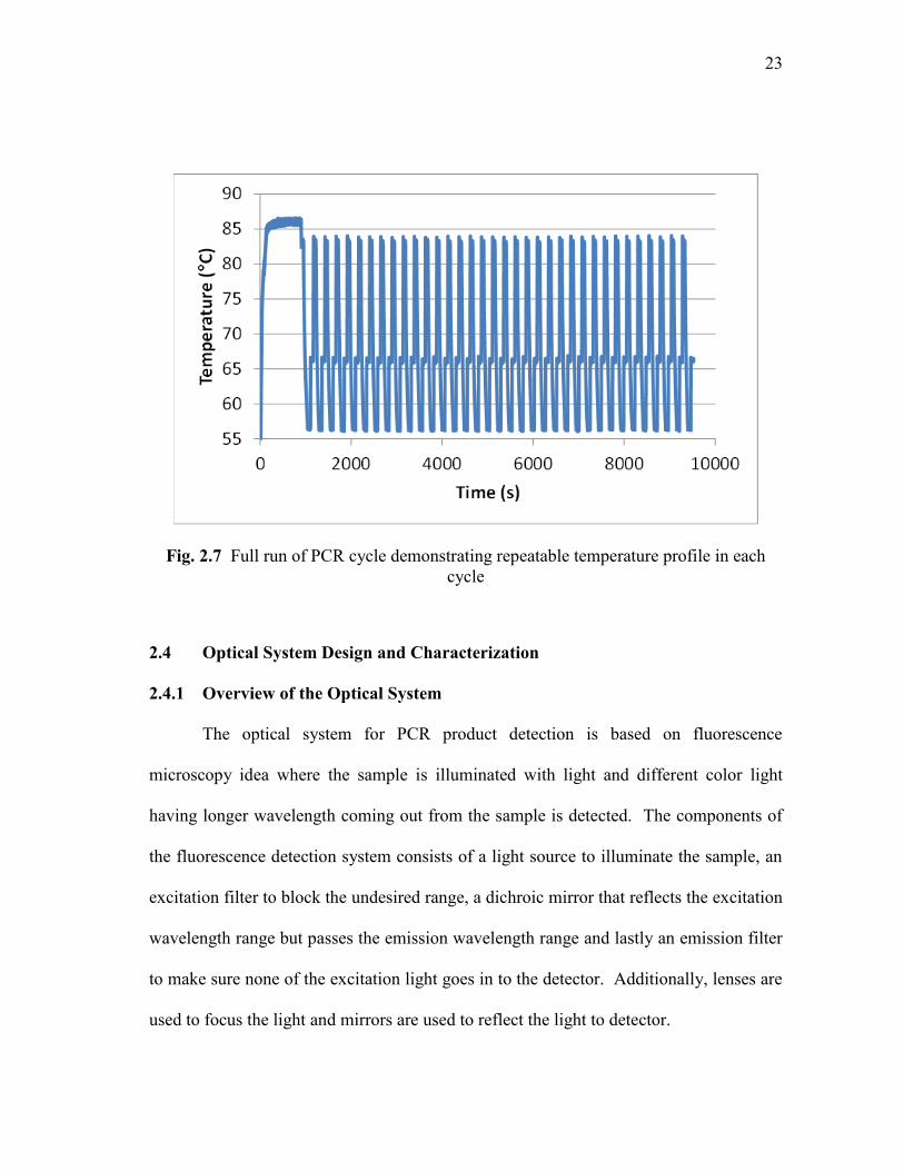
2.4 Optical System Design and Characterization
2.4.1 Overview of the Optical System
The optical system for PCR product detection is based on fluorescence
microscopy idea where the sample is illuminated with light and different color light
having longer wavelength coming out from the sample is detected. The components of
the fluorescence detection system consists of a light source to illuminate the sample, an
excitation filter to block the undesired range, a dichroic mirror that reflects the excitation
wavelength range but passes the emission wavelength range and lastly an emission filter
to make sure none of the excitation light goes in to the detector. Additionally, lenses are
used to focus the light and mirrors are used to reflect the light to detector.

24
In this work, SYBR Green dye is present in the PCR buffer and has a peak
excitation of 497 nm and peak emission of 520 nm. A blue LED NSPB310B (Nichia,
Tokushima, Japan) which has a dominant wavelength of 470 nm is used. To illuminate
the blue LED under constant current, LM317 integrated circuit (National
Semiconductor, Santa Clara, CA) is used with 180Ω resistor to have current of 7 mA.
The excitation filter used is ET470/40x (Chroma Technologies, Brattleboro, VT) which
passes the light between 450 and 490 nm only. After the excitation filter, the light is
focused with a lens having 14.9 mm focal length and 12.7 mm diameter (ThorLabs,
Newton, NJ) and hits a dichroic mirror that lies 45° to the ground (495dclp, Chroma
Technologies) which reflects the blue light upwards to hit the sample. Before hitting the
sample, the light passes through an aspheric lens (ThorLabs) which is 6.7 mm in
diameter with a 0.68 numerical aperture (NA) and has a working distance of 1.76 mm.
As soon as the light hits the sample, fluorescence emission takes place and will pass
through the aspheric lens and goes towards dichroic mirror. The dichroic mirror will
reflect the blue light while passing the green light. The green light hits a silver mirror
that has a 25.4 mm diameter. Finally, the light is filtered with an emission filter
(ET535/50m, Chroma Technologies) to block all the light that has less than 510 nm
wavelength. The light is sensed by a photomultiplier tube (PMT) that is located at the
end of the optical system. The PMT employed in the experiment is 931A (Hamamatsu,
Hamamatsu City, Japan).
The optical housing for detection of PCR samples illustrating the trajectory of the
blue and green light is shown in Fig. 2.8.
25
Fig. 2.8 The optical housing schematic used in fluorescence measurement. The blue ray
is the trajectory of the LED and the green ray is the trajectory of the fluorescent light
coming from the sample
2.4.2 Optical Housing Production and Microdevice Integration
To hold the optical components, an optical housing is made using 3D printer
(envisionTEC Ultra, Marl, Germany). The appropriate scheme was drawn in
SolidWorks software (Dassault Systems, Waltham, MA), modified in 3D printer

26
software to generate appropriate image files and transferred to the machine. 3D printer
has a light sensitive resin and selectively reflects the light just like a projector and light
solidifies the resin. The stage moves up and a new image file is loaded to 3D printer. In
this fashion, truly 3D structures can be produced in layer-by-layer fashion. The overall
size of the optical housing is 3.9 x 5.9 x 11.9 mm. All the parts reside inside the housing
except for the PMT which is tightly attached to the housing. The fabricated optical
housing with the structures is shown in Fig. 2.9.
Fig. 2.9 Manufactured optical housing using 3D printer. The LED is placed inside the
housing and green septa rubbers are used to seal the inlet and outlet of the microdevice

27
The integration of the PCR chip is accomplished by using gastight rubbers
(ThermoGreenTM
LB-2, Sigma-Aldrich, St. Louis, MO) on both sides of the
microdevice. After placing a cover layer with rubbers, screws are used to ensure a tight
sealing and avoid evaporation of the sample.
2.4.3 Optical Characterization of the System
The efficiency of the optical housing is tested using a spectrophotometer to
ensure appropriate excitation of the sample and reliable reading from the detector
location. Three different conditions are tested: LED’s wavelength, the excitation filter
output while the LED is on and reading from the detector location part of the optical
housing. The relative intensities of the three conditions are shown (Fig. 2.10).
According to the spectrophotometer results, the LED has some 500 nm or more
wavelengths which might affect the fluorescence efficiency but it is efficiently blocked
by the excitation filter. Finally, the reading from the detector part reveals that only
fluorescence part is detected by the detector and no blue light is present in that location.

28
Fig. 2.10 Spectrophotometer results showing suitable excitation and emission optical
components. The excitation filter blocks out the green light coming from the LED and
only green light range is observed from the output

29
2.4.4 Characterization of Fluorescence Detection Capability of the System
The optical system has been characterized in two ways. Firstly, a test involving
concentrations of Fluorescein isothiocyanate (FITC) ranging from 0 nM (DI water) to
2500 nM was done. For this purpose, an etched chamber layer is bonded to a plain glass
of same size and small (2 x 2 mm) Polydimethylsiloxane (PDMS) slabs including holes
were bonded on top of the inlet and outlet using plasma treatment. Tubing was attached
to inlet and outlet parts of the microdevice and desired concentration was injected into
the device using a syringe. Second characterization was done using PCR samples to
observe the difference between amplified and unamplified samples. Unamplified sample
was mixed and measured using the same fashion and amplified sample was
conventionally amplified using thermocycler before measurement. The graph for both
experiments is shown in Fig. 2.11.

30
Fig. 2.11 PMT characterization using fluorescent dye and PCR samples. Linear increase
in PMT output was observed for different dye concentrations. Additionally, unamplified
and amplified sample resulted in different PMT outputs making it suitable for PCR
experiments
As seen in the graph, the FITC concentrations gave a linear increase throughout
the experiment. Additionally, there was a 25 mV increase from unamplified to amplified
sample. Based on these finding, the optical system is considered to be efficient for PCR
experiments.
2.5 Developments towards a Multi Chamber Microchip PCR Design
After having achieved a heater design capable of generating a uniform
temperature distribution which is a good candidate for PCR experiments, additional
heater designs were considered for smaller chamber dimensions. The aim was to
squeeze three or four heaters in a 25.4 x 25.4 mm glass slide instead of one. The

31
chamber size becomes 3.5 x 6.5 mm. Several designs that are capable of heating the
sample inside the chambers were made and tested.
Firstly, the square spiral design was tested after reducing the size of the design
and connecting the four square spiral designs by a straight channel. The resulting
temperatures inside individual chambers are within several degrees however, there are
significant temperature differences between the temperatures of different chambers.
To overcome this problem, unconnected heater designs were considered. One
design has four bar shape heaters to heat four small size chambers. The heaters are in 21
x 5 mm with additional pads for soldering. Voltage is applied from pads and to all of the
heaters, which is running four heaters at the same time. A uniform temperature
distribution was observed around where the chamber would be located and is shown in
Fig. 2.12. The chambers in the middle and the chambers at the edges have the same
temperature range that differs from the other group.

32
Fig. 2.12 Simulation result of 4-bar design. Similar profile was observed from middle
chambers and edge chambers but the two groups have different temperature profile
However, an issue of this design is that the heaters have a low resistance. When
fabricated, it is observed that one heater draws around 1 Ampere at 2 Volts and running
even two heaters at the same time would require 2 Amperes which is a substantial
increase compared to the single chamber design where the drawn current is less than 0.5
Ampere. Based on this finding, simulations running one heater at a time were done and
found out especially the edge chambers have a non-uniform temperature distribution and
avoid successful PCR runs. The edge chamber simulation is shown in Fig.2.13.

33
Fig. 2.13 Simulation of one chamber in 4-bar design. The temperature difference within
the chamber is up to 5 degrees
Another issue with the four design heater is the reference point where the
thermocouple is located is very sensitive to temperature distribution if the reference
point is placed at the back side of the device slightly off the chamber to avoid spanning
the optical reading area. It can also be seen on the simulation result that the temperature
drops fast on the corners of the chamber (Fig.2.13). Moving the thermocouple by
several millimeters changes the temperature difference between the top of heater and
reference point significantly. Temperature profile of the individual four-bar heater was
done the same way as before, that is placing one thermocouple on top of the heater and
the other thermocouple on the back side on a reference point that is slightly off the
chamber. The temperature profile is shown in Fig. 2.14 and the temperature differences
between two points are 14°C for denaturation, 8°C for extension and 4°C for annealing
temperature. However, the temperature differences varied from experiment to
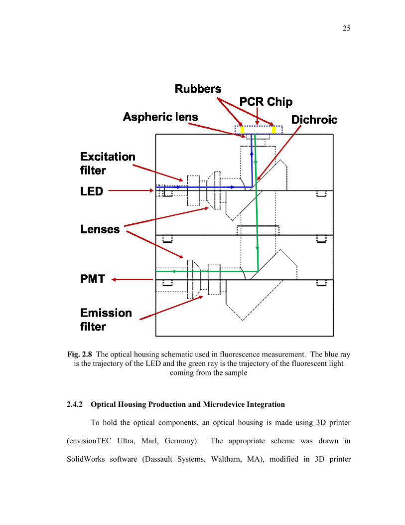
34
experiment because of placing the reference thermocouple slightly closer or to farther
from the chamber.
Fig. 2.14 Temperature profile of the 4-bar design. The difference between two
thermocouples is significant and since the reference thermocouple is very sensitive to
location there is a run to run variance in this experiment
The problems with the four-bar heater design led to seek for a better design that
has a better temperature uniformity when running individual chambers. So, a design to
have a higher resistance was designed which is a serpentine shape design that covers the
area of individual chambers. The serpentine heater is 19.4 x 5 mm in size while each leg
of the heater is 500 µm thick and the gap of each leg is 200 µm. Both middle chamber
and edge chambers were simulated while the water is introduced in the chamber. The
middle chamber temperature is within 2 degrees and good uniformity is observed. On
the other hand, the edge chamber temperature while within several degrees has a slightly
0
20
40
60
80
100
0 500 1000 1500 2000 2500
Tem
pe
ratu
re ( C
)
Time (s)
Heater
Reference

35
shifted temperature gradient but it is considered as good enough for PCR thermocycling.
The simulation of both cases is shown in Fig. 2.15.
Fig. 2.15 Temperature simulations of serpentine design. Top views of (A) middle and
(B) edge chamber are shown. The temperature inside the chamber is within 2 degrees

36
Observing good uniformity in simulations of the serpentine design, it was
fabricated (Fig. 2.16) and temperature profile was tested using two thermocouples
attached on top of the heater and at the back side of the heater after fabricating the
microdevices. The main reason to change the position of the reference point is to avoid
having a big temperature difference by slightly moving the thermocouple. The
temperature profile is shown in Fig. 2.17 and the temperature differences between two
thermocouples are 4.5°C for denaturation, 2.5° for extension and 1.5° for annealing
temperature. The experiment was repeated several more times and low experiment to
experiment variation was observed.
Fig. 2.16 Fabricated serpentine design microdevice

37
Fig. 2.17 Temperature profile of the serpentine design. There is a small difference
between two thermocouples and the variance from run to run is small
The serpentine design gave a better performance in terms of drawn current (0.2
A) and temperature uniformity and it was decided to use serpentine design for multiple
chamber microdevices. The thermocouple was decided to be placed on top of the heater
during the PCR thermocycling and the set temperatures are determined to be 96.5°C for
hot-start, 95.5°C for denaturation, 73°C for extension and 61°C for annealing
temperature.
50
60
70
80
90
100
0 500 1000 1500 2000 2500
Tem
pe
ratu
re ( C
)
Time (s)
Heater
Back

38
CHAPTER III
DEVELOPMENT OF THE PORTABLE PATHOGEN DETECTION LAB ON A CHIP
(PADLOC)
3.1 Overview of the PADLOC System
The PADLOC system is composed of three subsystems. These are
microfabricated PCR chip with integrated heater, a fluorescence detection system and a
controller system. The thermocycling of the sample is done by the heater on the PCR
chip while controlled by a controller system that is hooked up to a computer and
thermocouple is used as a temperature sensor. The controller system also arranges the
timing of light source and recording of optical detector. The overall structure of the
PADLOC system is shown in Fig. 3.1.
Fig. 3.1 Overall view of PADLOC system having microdevice, optical setup and
control and acquisition modules

39
3.2 System Control and Operation
The control of thermocycling and optical excitation and detection is done using
NI LabVIEW software. LabVIEW is the software of choice when working on data
acquisition. With additional hardware modules, it is possible to read, write, manipulate
and output physical quantities such as voltage, current, resistor, temperature, stress,
strain, etc. A general outline of the LabVIEW software used in PADLOC system is
shown in Fig. 3.2.
Fig. 3.2 The structure of the Labview program for PCR experiments. It can be regarded
as a combination of two programs: One for temperature control and one for data
acquisition and display

40
Three different NI modules are used in the system. These are NI 9481 which is a
relay module that transmits or rejects the supplied voltage according to control
parameters, NI 9211 which is a thermocouple input module to sense the temperature of
the sample and NI 9205 module which is a voltage input module used to read PMT
voltage. All these modules are located on a NI 9172 chassis. The relay module is used
to control the thermocycling of the PCR chip as well as to turn on the LED on the last
second of extension temperature zone. The PMT input voltage is read differentially
meaning that two cables are connected to the voltage input module and it reads the
difference of the two wires. The wires are coming from positive and negative output of
the PMT.
The software first initializes the relay module and creates a counter that controls
the timing of the PCR experiment. After creating a counter and a virtual channel, hot-
start part of the experiment starts. The software goes into a loop of heating the sample to
hot-start temperature until the specified time (in our experiments it is 15 minutes) is
over. While the program is in the loop it also executes PID control using the internal
PID functions of NI LabVIEW PID and Fuzzy Logic Toolkit add-on. Following hot-
start, the software executes thermocycling of denaturation, annealing and extension
temperature zones in a loop similar to hot-start. The three temperature zones are
alternated until the desired cycle (usually 35 cycles in our experiments) is completed and
relay module turns on the LED on the last second of the extension zone for each cycle.
While the relay module accomplishes the thermocycling and LED excitation based on
the software, the voltage and temperature input modules create channels for temperature

41
and voltage in a similar fashion. The input tasks are started at the same time as relay
module. The temperature input is read continuously during the PCR experiment in a
loop and the temperature data is written to a file. The voltage input is read for only one
second in each cycle since the LED illuminates the sample in that specific second in
order to avoid photobleaching of the PCR sample. The voltage data is also written to a
separate file. The temperature and PMT output is also displayed on the PC screen on the
front-end of the LabVIEW program. The front-end includes selection of temperature
durations, cycle times and file selection for temperature and voltage data as well as
graphs for temperature and voltage data. The front-end of the LabVIEW program is
shown in Fig. 3.3.
Fig. 3.3 Front-end of the Labview program. It allows entering temperature durations
and files to log the data as well as displays temperature and PMT output data

42
3.3 Specifications of the System
The PCR chips used in the experiments have 200 Å Cr and 1800 Å Au layer and
they have around 30Ω resistance for square spiral design and 100Ω resistance for
serpentine design. The applied voltages to the heaters are between 10 and 15 V.
On the optical detection side, a constant current source integrated circuit (IC) is
used to ensure same light excitation intensity in every cycle. An 180Ω resistor is
connected in between the IC’s legs to have a current of 7 mA. The LabVIEW software
is set to read 14 samples per second which is the maximum limit for temperature input
module. The PMT is powered to 14.3 V using a power supply (mastech, Pittsburg, PA).
In the voltage measurement file, 14 samples are output for each cycle since the voltage is
read for only one second when LED is on. The first five values for each cycle are
discarded since the LED intensity doesn’t reach its full brightness right after it is on and
results in low output reading. The remaining samples are averaged using Microsoft
Excel software and the voltage increase is plotted against cycle number.
The size of the optical housing is 3.9 x 5.9 x 11.9 mm including the PMT and the
overall size of the NI modules are 250 x 85 x 90 mm. Additionally, a small part of a
breadboard is used for constant current source circuitry, power supplies for heater, LED
and PMT. Lastly, a computer is used to run LabVIEW software. The system itself
without computer and power supplies uses small space and is portable.
PADLOC system performance is compared to a conventional thermocycler that
can be found in plant pathology labs using the same pathogen and PCR kits. The heating

43
and cooling times of the thermocycler are included together but are given separately in
our work. The table is shown in Table 3.1.
Table 3.1 PADLOC system and thermocycler temperature durations
This work Conventional Thermocycler
Hot-start 915 s 900 s
Denaturation 48.5s x 35 = 1697.5 s 15s x 35 = 525 s
Annealing 59s x 35 = 2065 s 30s x 35 = 1050 s
Extension 58s x 35 = 2030 s 30s x 35 = 1050 s
Warm up 557 s
2475 s
Cool down 2471 s
Total 2 h 42 min 1 h 40 min
3.4 Sample and Reagents
Before starting the PCR experiment, both the rubbers and PCR microdevice are
sterilized using autoclave in order to avoid any contamination problems. The devices
are coated with Bovine Serum Albumin (BSA) having concentration 10 mg/ml for 15
minutes in order to avoid adsorption of the sample on the microdevice walls.
Afterwards, the BSA inside the chamber is sucked and prepared sample is loaded inside
the chamber.
The samples are stored at -20°C and they are thawed on ice before preparation.
A 20 µl sample is prepared using 10 µl of Sybr Green PCR master mix (Qiagen,
Valencia, CA), 5 µl RNase –free water, 1 µl forward and reverse primers having5'- TCG

44
TTT CCA GGA AAG CTG C -3' and 5'- GCA GCT TTC CTG GAA ACG A -3' , 1 µl
10% Polyvinylpyrrolidone (PVP) and 1 µl 1 mg/ml BSA. The sample in the tube was
mixed using a vortex mixer for several seconds and injected into the BSA-treated
chamber.
3.5 Detection of Pure Genomic DNA
3.5.1 Detection using PADLOC and Validation
PCR experiments were done using pure fungal genomic DNA to amplify part of
SIX1 gene from Fusarium oxysporum spf. lycopersici. The total PCR experiment has a
15 minute hot-start following a 35 cycle of three temperature zones for 50, 60 and 60
seconds. After averaging the samples as described in specifications section, Excel plots
are obtained and are shown in Fig.3.4.
According to the PMT output, an expected increase in PMT voltage was
observed. The voltage profile of the experiment in the presence of target DNA showed
an obvious increase in the fluorescence of the sample which was expected.
Fig. 3.4 PMT outputs of three PCR runs. The fluorescence intensity increases were
shown

45
To verify the PCR amplification results, gel electrophoresis was also done after
the experiment. The sample was extracted using a pipette and loaded in 1.2% agarose
gel. After preparing the agarose in 0.5x TBE buffer and boiling in microwave oven for
50 seconds, the mixture was left for solidification. The gel was run in 0.5x TBE buffer
at 95 V for around 50 minutes. For PCR ladder, 7 µl 1Kb PCR ranger (GenDEPOT,
Barker, TX) was loaded in the first well. Before loading the sample, they are mixed with
6x loading dye (New England Biolabs, Ipswich, MA). Following the 50 minute voltage
exposure, the gel was taken out of the buffer and the picture was taken as the gel was
illuminated with a UV light. The gel pictures of several runs are shown in Fig.3.5. The
first well was filled with DNA ladder to visually see the base pair length (bp) of the
sample. The bands were observed between 200 and 300 bp and the target DNA is 260
bp in length. This result verifies the selective amplification of the target DNA.

46
Fig. 3.5 Gel electrophoresis results of PCR runs. The bands are observed between 200
and 300 bp. The first well is filled with DNA ladder to aid in visualization of the bands
3.5.2 Evaluation of Repeatability and Success Ratio
The amplification of pure fungal genomic DNA was tested repeatedly to ensure
proper functioning of the PADLOC system. Many PCR runs (10) were done and both
PMT output voltages and gel electrophoresis results were compared. In all of the runs,
bands were observed in correct location in gel electrophoresis. In most of the runs,
fluorescence intensity detection using the PMT was also included. According to the
results, in several of the runs the PMT voltage increase as the PCR cycles increased were

47
not significant. The problem is caused by inherent drift in PMT. As time passes by, the
PMT outputs less voltage under the same conditions. The PMT can be warmed-up by
applying voltage for a certain amount of time before the experiment starts to reduce the
drift. In the PCR experiments, the PMT was used without warming up and caused drift
in the output voltage.
The drift in PMT was characterized by measuring the PMT voltage while the
chamber was empty. Without warming-up the PMT, the drift was found out to be
around 8.75% at the end of the experiment. With a 60 minute warm-up period the drift
dropped down to 1.5% at the end of the experiment. Under the light of these findings, it
was concluded that the drop in PMT voltage was caused by the drift in PMT and this
problem can be improved significantly by warming-up the PMT before the experiment.
3.6 Multichamber Design Results
The PCR experiment was tested using the serpentine design small chambers. All
the conditions including sample preparation, BSA coating, cycle times, and optical
housing integration were the same. There are two differences from big chamber design.
They are additional autoclaved PDMS slabs inclusion to seal the inlet and outlet and the
temperature values were different. The set temperatures were obtained in serpentine
design calibration as mentioned in Section 2.5. The drift in the PMT was also taken into
account as opposed to previous big chamber experiments. A PCR run using an empty
chamber was done and the results were accounted to have a constant output. The values
then were applied to PCR experiment. The resulting PMT output graph is shown in

48
Fig.3.6. Since the volume for the small chamber is small and we previously confirmed
from big chamber designs that when we observe an increase in PMT output, we also
observed a band in correct location in gel electrophoresis verification.
Fig. 3.6 The PMT output graphs of serpentine design. The increases in signal intensity
are shown
The fluorescence intensities increased which was attributed to amplification of
DNAs during the thermocycling.
49
CHAPTER IV
SUMMARY AND FUTURE WORK
4.1 Project Review
In this work, we developed and utilized a miniaturized real-time quantitative
PCR system that can be used to diagnose plant pathogens.
The system is comprised of three sub-systems. The first sub-system is a
microfabricated PCR chip to hold the PCR sample inside that is made of glass with gold
layer on top to accomplish thermocycling of the sample. The second sub-system is a
fluorescent intensity detector that employs LED, lenses, mirrors, dichroic mirror and
PMT for fluorescent excitation and collection. The optical components are placed in a
housing to ensure proper alignment of the components and avoid light leakage. The
selection of LED as a light source and small PMT as an optical detector allows us to
have a portable system with low power requirements. Lastly, the third system is NI
Labview software and modules to read and display temperature and voltage data as well
as control the temperature using PID control via a thermocouple.
The PCR chip has two different designs based on their high-throughput needs. A
square spiral design was used to heat up a relatively large chamber that holds enough
PCR sample to run gel electrophoresis and serpentine heater design was used to increase
the high throughput of the system. Three serpentine heaters were placed in 25.4 x 25.4
mm PCR chip having three chambers. The designs were checked for uniform heating
using COMSOL Multiphysics® software before fabricating. The optical detection

50
system is characterized before starting the PCR experiments using spectrophotometer for
accurate and efficient excitation and emission wavelengths. Additionally, the optical
detection system was characterized using increased concentrations of fluorescent dye
that has similar characteristics as PCR sample.
The PADLOC system was tested using pure fungal genomic DNA that affects
some crops such as tomato. The detection was done in real-time thanks to the optical
system while thermocycling of the sample takes place. Additionally, for the big
chamber design gel electrophoresis verification was done after the end of the
experiment. Both PMT output voltage and gel electrophoresis results showed that our
PADLOC system achieved detection of plant pathogen DNA.
4.2 Future Work
There are two aspects of our PADLOC system that can be advanced. These
aspects are application side and device side. On the application side, the
accomplishment of the PADLOC system has enabled further pathogen detection
possible. In this work, the DNA used in the experiments was pure fungal genomic
DNA. As future work, the target DNA will be changed to DNAs that are extracted from
tomato plants. Those DNAs will have both tomato and fungal DNA if the plant is
infected. The DNAs will be obtained from our collaborator Dr. Shim’s lab. We believe
the detection of extracted DNA will enable on-site detection thanks to the portability of
our PADLOC system.

51
On the device side, the multiple chamber design has been run individually so far.
The system will be modified to enable multiplex detection of three samples at the same
time. For this goal, optical housing will be modified slightly. There will be three LEDs
and three aspheric lenses to individually focus light into each chamber. The LEDs will
turn on and off sequentially at the last seconds of extension zone. The filters, lenses and
dichroic mirror will be kept the same. Thus, by employing the current setup as much as
possible the optical system will be used for multiplex detection of PCR samples.
52
REFERENCES
1 Agriculture, U.S.D. National Program 303: Plant Diseases. 2010 [cited 2012;
Available from:
http://www.ars.usda.gov/research/programs/programs.htm?np_code=303&docid
=12682.
2 R. K. Saiki, S. Scharf, F. Faloona, K. B. Mullis, G. T. Horn, H. A. Erlich and N.
Arnheim ,Science, 1985. 230(4732): p. 1350-1354.
3 F. C. Lawyer, S. Stoffel, R. K. Saiki, K. Myambo, R. Drummond and D. H.
Gelfand , Journal of Biological Chemistry, 1989. 264(11): p. 6427-6437.
4 C. J. Easley, L. A. Legendre, J. P. Landers and J. P. Ferrance, Microchip
Capillary Electrophoresis : Methods and Protocols, 2006. 339: p. 217-231.
5 R. Higuchi, G. Dollinger, P. S. Walsh and R. Griffith , Bio-Technology, 1992.
10(4): p. 413-417.
6 C. A. Heid, J. Stevens, K. J. Livak and P. M. Williams, Genome Research, 1996.
6(10): p. 986-994.
7 C. S. Zhang, J. L. Xu, W. L. Ma and W. L. Zheng, Biotechnology Advances,
2006. 24(3): p. 243-284.
8 M. A. Northrup, M. T. Ching, R. M. White and R. T. Watson, Tranducer'93
Seventh International Conference on Solid State Sens Actuators. 1993.
Yokohama, Japan.

53
9 A. T. Woolley, D. Hadley, P. Landre, A. J. deMello, R. A. Mathies and M. A.
Northrup, Analytical Chemistry, 1996. 68(23): p. 4081-4086.
10 R. C. Anderson, X. Su, G. J. Bogdan and J. Fenton,Nucleic Acids Research,
2000. 28(12).
11 T. B. Taylor, E. S. WinnDeen, E. Picozza T. M. Woudenberg and M. Albin,
Nucleic Acids Research, 1997. 25(15): p. 3164-3168.
12 P. Belgrader, J. K. Smith, V. W. Weedn and M. A. Northrup, Journal of Forensic
Sciences, 1998. 43(2): p. 315-319.
13 S. Poser, T. Schulz, U. Dillner, V. Baier, J. M. Kohler, D. Schimkat, G. Mayer
and A. Siebert, Sensors and Actuators A-Physical, 1997. 62(1-3): p. 672-675.
14 M. U. Kopp, A. J. de Mello and A. Manz, Science, 1998. 280(5366): p. 1046-
1048.
15 P. Gascoyne, J. Satayavivad and M. Ruchirawat, Acta Tropica, 2004. 89(3): p.
357-369.
16 J. West, B. Karamata, B. Lillis, J. P. Gleeson, J. Alderman, J. K. Collins, W.
Lane, A. Mathewson and H. Berney, Lab Chip, 2002. 2(4): p. 224-230.
17 J. Liu, M. Enzelberger and S. Quake, Electrophoresis, 2002. 23(10): p. 1531-
1536.
18 A. L. Markey, S. Mohr and P. J. R. Day, Methods, 2010. 50(4): p. 277-281.
19 I. Kobayashi, K. Uemura and M. Nakajima, Colloids and Surfaces A-
Physicochemical and Engineering Aspects, 2007. 296(1-3): p. 285-289.
20 D. Braun, Modern Physics Letters B, 2004. 18(16): p. 775-784.
54
21 M. Krishnan, V. M. Ugaz and M. A. Burns, Science, 2002. 298(5594): p. 793-
793.
22 M. Q. Bu, T. Melvin, G. Ensell, J. S. Wilkinson and A. G. R. Evans, Journal of
Micromechanics and Microengineering, 2003. 13(4): p. S125-S130.
23 J. El-Ali, I. R. Perch-Nielsen, C. R. Poulsen, D. D. Bang, P. Telleman and A.
Wolff, Sensors and Actuators A-Physical, 2004. 110(1-3): p. 3-10.
24 C. S. Liao, G. B. Lee, J. J. Wu, C. C. Chang, T. M. Hsieh, F. C.Huang and C. H.
Luo, Biosensors & Bioelectronics, 2005. 20(7): p. 1341-1348.
25 I. Rodriguez, M. Lesaicherre, Y. Tie, Q. B. Zou, C. Yu, J. Singh, L. T. Meng, S.
Uppili, S. F.Y. Li, P. Gopalakrishnakone and Z. E. Selvanayagam,
Electrophoresis, 2003. 24(1-2): p. 172-178.
26 D. J. Sadler, R. Changrani, P. Roberts, C. F. Chou and F. Zenhausen, Itherm
2002: Eighth Intersociety Conference on Thermal and Thermomechanical
Phenomena in Electronic Systems, Proceedings, 2002: p. 1025-1032.
27 Q. B. Zou, U. Sridhar, Y. Cheng and J. Singh, Ieee Sensors Journal, 2003. 3(6):
p. 774-780.
28 T. Fukuba, T. Yamamoto, T. Naganuma and T. Fujii, Chemical Engineering
Journal, 2004. 101(1-3): p. 151-156.
29 L. Erill, S. Campoy, J. Rus, L. Fonseca, A. Ivorra, Z. Navarro, J. A. Plaza, J.
Aguilo and J. Barbe, Journal of Micromechanics and Microengineering, 2004.
14(11): p. 1558-1568.

55
30 V. P. Iordanov, J. Bastemeijer, A. Bossche, P. M. Sarro, M. Malatek, I. T.
Young, G. W. K. van Dedem and M. J. Vellekoop, Proceedings of the Ieee
Sensors 2003, Vols 1 and 2, 2003: p. 1045-1048.
31 H. Yang, C. A. Choi, K. H. Chung, C. H. Chun and Y. T. Kim, Analytical
Chemistry, 2004. 76(5): p. 1537-1543.
32 A. Gulliksen, L. Solli, F. Karlsen, H. Rogne, E. Hovig, T. Nordstrom and R.
Sirevag, Analytical Chemistry, 2004. 76(1): p. 9-14.
33 P. J. Obeid and T.K. Christopoulos, Analytica Chimica Acta, 2003. 494(1-2): p.
1-9.
34 Z. M. Zhou, D. Y. Liu, R. T. Zhong, Z. P. Dai, D. P. Wu, H. Wang, Y. G. Du, Z.
N. Xia, L. P. Zhang, X. D. Mei and B. C. Lin, Electrophoresis, 2004. 25(17): p.
3032-3039.
35 C. J. Bruckner-Lea, T. Tsukuda, B. Dockendorff, J. C. Follansbee, M. T.
Kingsley, C. Ocampo, J. R. Stults and D. P. Chandler, Analytica Chimica Acta,
2002. 469(1): p. 129-140.
36 Y. Matsubara, K. Kerman, M. Kobayashi, S. Yamamura, Y. Morita and E.
Tamiya, Biosensors & Bioelectronics, 2005. 20(8): p. 1482-1490.
37 M. W. Mitchell, X. Z.Liu, Y. Bejat, D. E. Nikitopodoulos, S. Soper and M. C.
Murphy, Microfluidics, Biomems, and Medical Microsystems, 2003. 4982: p. 83-
98.
38 C. G. Koh, W. Tan, M. Q. Zhao, A. J. Ricco and Z. H. Fan, Analytical
Chemistry, 2003. 75(22): p. 6379-6379.

56
39 M. Curcio and J. Roeraade, Analytical Chemistry, 2003. 75(1): p. 1-7.
40 P. Sethu and C. H. Mastrangelo, Sensors and Actuators B-Chemical, 2004. 98(2-
3): p. 337-346.
41 X. M. Yu, D. C. Zhang, T. Li, L. Hao and X. H. Li, Sensors and Actuators A-
Physical, 2003. 108(1-3): p. 103-107.
42 N. Krishnan, N. Agrawal, M. A. Burns and V. M. Ugaz, Analytical Chemistry,
2004. 76(21): p. 6254-6265.
43 N. Y. Zhang, H. D. Tan and E. S. Yeung, Analytical Chemistry, 1999. 71(6): p.
1138-1145.
44 A. F. R. Huhmer and J. P. Landers, Analytical Chemistry, 2000. 72(21): p. 5507-
5512.
45 J. P. Ferrance, Q. R. Wu, B. Giordano, C. Hernandez. Y. Kwok, S. Thibodeau
and J. P. Sanders, Analytica Chimica Acta, 2003. 500(1-2): p. 223-236.
46 D. Pal and V. Venkataraman, Sensors and Actuators A-Physical, 2002. 102(1-2):
p. 151-156.
47 K. Orrling, P. Nilsson, M. Gullberg and M. Larhed, Chemical Communications,
2004. 7: p. 790-791.
48 C. Fermer, P. Nilsson and M. Larhed, European Journal of Pharmaceutical
Sciences, 2003. 18(2): p. 129-132.
49 R. M. Guijt, A. Dodge, G. W. K. van Dedem, N. F. de Rooij and E. Verpoorte,
Lab Chip, 2003. 3(1): p. 1-4.

57
50 S. Stern, C. Brooks, M. Strachan, A. Kopf-Sill and J. W. Parce, Itherm 2002:
Eighth Intersociety Conference on Thermal and Thermomechanical Phenomena
in Electronic Systems, Proceedings, 2002: p. 1033-1038.
51 W. C. Dunn, S. C. Jacobson, L. C. Waters, N. Kroutchinina, J. Khandurina, R. S.
Foote, M. J. Justice, L. J. Stubbs and J. M. Ramsey, Analytical Biochemistry,
2000. 277(1): p. 157-160.
52 J. Khandurina, T. E. McKnight, S. C. Jacobson, L. C. Waters, R. S. Foote and J.
M. Ramsey, Analytical Chemistry, 2000. 72(13): p. 2995-3000.
53 E. T. Lagally, J. R. Scherer, R. G. Blazej, N. M. Toriello, B. A. Diep, M.
Ramchandani, G. F. Sensabaugh, L. W. Riley and R. A. Mathies, Analytical
Chemistry, 2004. 76(11): p. 3162-3170.
54 R. Drmanac, S. Drmanac, Z. Strezoska, T. Paunesku, I. Labat, M. Zeremski, J.
Snoddy, W. K. Funkhouser, B. Koop, L. Hood and R. Crkvenjakov, Science,
1993. 260(5114): p. 1649-1653.
55 R. H. Liu, J. N. Yang, R. Lenigk, J. Bonanno and P. Grodzinski, Analytical
Chemistry, 2004. 76(7): p. 1824-1831.
56 D. Trau, T. M. H. Lee, A. I. K. Lao, R. Lenigk, I. M. Hsing, N. Y. Ip, M. C.
Carles and N. J. Sucher, Analytical Chemistry, 2002. 74(13): p. 3168-3173.
57 H. Nagai, Y. Murakami, Y. Morita, K. Yokoyama and E. Tamiya, Analytical
Chemistry, 2001. 73(5): p. 1043-1047.
58 M. Krishnan, D. T. Burke and M. A. Burns, Analytical Chemistry, 2004. 76(22):
p. 6588-6593.

58
59 J. A. Higgins, S. Nasarabadi, J. S. Karns, D. R. Shelton, M. Cooper, A. Gbakima
and R. P. Koopman, Biosensors & Bioelectronics, 2003. 18(9): p. 1115-1123.
60 N. C. Cady, S. Stelick, M. V. Kunnavakkam and C. A. Batt, Sensors and
Actuators B-Chemical, 2005. 107(1): p. 332-341.
61 K. Sun, A. Yamaguchi, Y. Ishida, S. Matsuo and H. Misawa, Sensors and
Actuators B-Chemical, 2002. 84(2-3): p. 283-289.
62 Q. Xiang, B. Xu and D. Li, Biomedical Microdevices, 2007. 9(4): p. 443-449.
63 M. A. Northrup, B. Benett, D. Hadley, P. Landre, S. Lehew, J, Richards and P.
Stratton, Analytical Chemistry, 1998. 70(5): p. 918-922.
64 Z. Zhao, Z. Cui, D. F. Cui and S. H. Xia, Sensors and Actuators A-Physical,
2003. 108(1-3): p. 162-167.
65 Y. C. Lin, M. Li, M. T. Chung, C. Y. Wu and K. C. Young, Sensors and
Materials, 2002. 14(4): p. 199-208.
66 S. F. Li, D. Y. Fozdar, M. F. Ali, H. Li, D. B. Shao, D. M. Vykoukal, J.
Vykoukal, P. N. Floriano, M. Olsen, J. T. McDevitt, P. R. C. Gascoyne and S. C.
Chen, Journal of Microelectromechanical Systems, 2006. 15(1): p. 223-236.
67 P. Belgrader, S. Young, B. Yuan, M. Primeau, L. A. Christel, F. Pourahmadi and
M. A. Northrup, Analytical Chemistry, 2001. 73(2): p. 286-289.
68 Y. J. Liu, C. B. Rauch, R. L. Stevens, R. Lenigk, J. N. Yang, D. B. Rhine and P.
Grodzinski, Analytical Chemistry, 2002. 74(13): p. 3063-3070.

59
69 Y. K. Cho, J. Kim, Y. Lee, Y. A. Kim, K. Namkoong, H. Lim, K. W. Oh, S.
Kim, J. Han, C. Park, Y. E. Pak, C. S. Ki, J. R. Choi, H. K. Myeong and C. Ko,
Biosensors & Bioelectronics, 2006. 21(11): p. 2161-2169.
70 S. Julich, M. Riedel, M. Kielpinski, M. Urban, R. Kretschmer, S. Wagner, W.
Fritzsche, T. Henkel, R. Moller and S. Werres, Biosensors & Bioelectronics,
2011. 26(10): p. 4070-4075.
71 J. Kim and B. K. Gale, The 10th International Conference on Miniaturized
Systems for Chemistry and Life Sciences. 2006. Tokyo, Japan.
72 K. J. Astrom and T. Hagglund, Control Engineering Practice, 2001. 9(11): p.
1163-1175.
73 K. H. Ang, G. Chong, and Y. Li, Ieee Transactions on Control Systems
Technology, 2005. 13(4): p. 559-576.

60
APPENDIX A
COMSOL JOULE HEATING MANUAL
Overview
Joule Heating, also known as resistive heating is the phenomenon where a
conductor releases heat when electric current goes through it.
Example: Temperature Profile of a Chamber
1. Open COMSOL by double-clicking its icon. When the “Model Wizard”
opens, select a space dimension: 3D (Using 3D space produces the most
accurate results but reduced dimensions can be used to save time and
computation power).
2. In the “Add physic” window, click the heat transfer folder, then click “joule
heating (jh)”. Click the next arrow button.
3. In the “Select study type” window, you can choose stationary for the steady-
state position or time dependent to see the physics in your model at the
specified times. Then click the finish button.
4. Click “Geometry1” in the “Model builder” window, and change the length
unit to an appropriate scale. (µm in this example)
Drawing
5. There are two different ways to make your model in Comsol. The first one is
to draw your model in CAD software and save as .dxf file. You can import
your model into Comsol by right clicking “Geometry1” and import. Right

61
after the import you can use the “zoom extents” button on the “Graphics”
toolbar to see the whole design in appropriate scale. After importing, you can
extrude and finish the design forming union. (Will be described) In the case of
having to use a complicated design, it is better draw the design in a CAD
software and import to Comsol since Comsol without CAD module is not very
user-friendly and has limited geometry selections.
6. To draw a microchamber device consisting of a patterned and etched glass
sheet and a glass sheet with Au electrode on top, right click to “Geometry1”
and select work plane and click build selected on top toolbar. Now the
drawing panel is ready when you go to “Geometry” under the “Geometry1”
menu on the left part of the screen. Click “draw square (center)” and enter the
value of 25400 µm as side length, x, 0 µm, and y, 0 µm as center coordinates.
Right-click “Geometry1” and click “rectangle” and enter the value of Width,
20000 µm, Height, 5000 µm, x, -10000 µm, and y, 5000 µm for the corner.
Then, add two “square (center)” with the side length of 1000 µm. The center
coordinates are y, 7500 µm and x, 10500 and -10500 µm. For the chamber
part, click “ellipse (center)” and use the values a-semi axis, 6000 µm, b-semi
axis, 2000 µm, x, 0 µm and y, 7500 µm.
7. After drawing all the shapes, it is time to give the objects third dimension
which can be done by extruding and using Boolean operations. Right click the
work plane and select extrude, select the eclipse check the reverse direction to
extrude in the other direction and enter 80 µm.

62
8. Right click on the work plane and select extrude again. Select the square and
extrude 500 µm in reverse direction.
9. In the same fashion, select the remaining shapes (three rectangles) and extrude
600 µm. (In regular direction)
10. In the work plane, draw the same square (25400 µm side length) that was
drawn first (Explained in step 6). It may be harder to select this square if it is
drawn before extrusion processes so that is the reason why it is drawn now.
Extrude this 500 µm.
11. Right click “Geometry1” and select Boolean operation Difference. In the
“Objects to add” include the three rectangles while in the “Objects to subtract”
select the “sq4” that is the last square drawn. Click build selected and this will
create a hanging electrode design.
12. Draw a square identical to “sq4” and extrude 500 µm to have a complete
design.
13. Click “Form Union” to finalize your drawing. Alternatively, you can use
“Form Assembly” to have a manual control on the boundaries and the physics.
However, forming union is a convenient and more automated approach. The
finalized drawing is shown below.

63
Fig. A.1 Finalized Drawing of Heater
Materials
14. Now that we have a complete drawing, we can assign materials to the
drawings. For this purpose, locate the “Model builder” window, right-click
“Materials” and select “Open Material Browser”
15. In the “Material Browser”, expand the “Built-in” folder, locate Silica Glass,
right-click and select “Add Material to Model”
16. Select domain 1 and 2 by first left clicking and then right clicking. The blue
color means the material has been applied to the highlighted domains.
17. Add gold the selection to domain 3, 4 and 6. Under the “Material Content”
part a stop sign on the left of the relative permittivity is shown. Put 1 here and

64
it turns into a green tick. Green tick means the value is ok, the stop sign means
the value is not valid and computation cannot be done.
18. To add material properties, click the material name under the material folder;
expand “Material Properties” in the “Material” window. Click “Basic
properties” and right-click the property which you want to add and select “add
to material”.
19. Finally, add water to selection and apply to domain 5. It cannot be seen
directly so you can press transparency button on the upper toolbar to have a
transparent drawing and you can select the domain 5. Use 80 as relative
permittivity of water. The material assignment is now finished and ready for
physics assignment.

65
Fig. A.2 Finalized Drawing of Microdevice
Physics
20. In the “Model Builder”, expand the “Joule Heating” node.
21. Right click on “Joule Heating” and select “Heat Transfer Heat Flux” on the
second part of the drop-down menu. This is the part where the affected
domains can be set. In our case all the boundaries except for the ground and
electric voltage applied boundaries will be affected. In the upper part of
middle menu, choose all boundaries and manually remove the domains 10 and
35. In the bottom part, click inward heat flux and use 10 as heat transfer
coefficient.

66
Fig. A.3 Application of Heat Flux
22. Right-click the “Joule Heating” in the “Model Builder”, click “Electric
Currents Ground” and select domain 10. This is where your ground will be.
23. Right-click the “Joule Heating” in the “Model Builder”, click “Electric
Currents Electric Potential” and select domain 35. Enter the applied
voltage here as 0.04 V
Meshing
24. Click “Mesh” In the “Model Builder”, select “Element size” and choose
coarse. Right click “Free Tetrahedral” and choose “Build All” to complete

67
meshing. Coarse meshing has fewer elements than normal so it takes less time
to compute. However, it is important to note that the accuracy drops as you
have coarser meshing.
Fig. A.4 Structure of the Device After Meshing
Study
25. To run a stationary simulation, right-click “study I” in the “Model Builder”
and choose “Compute”.

68
26. On the other hand, if you are running a time-dependent simulation, click
“study I” to expand and locate “Step 1: Time Dependent”. Click the button
next “Times” where you can select the start time, stop time and interval in
seconds. Afterwards, right-click “study I” in the “Model Builder” and choose
“Compute”
Results
27. Under “Results””3D Pilot Group1”, click the “Surface1”. In the “Settings”
window, click “Range” and select “Manual color range” to see the desired
interval on the surface.
Fig. A.5 3D Overview of Simulation

69
28. To see the cross section of the chamber, go to “3D Group2” and select the
slice. On the right menu, under “plane data” the cut direction can be chosen.
Afterwards, a number of equally spaced planes or an exact coordination plane
can be sliced. The cross-section of the chamber is shown below.
Fig. A.6 Cross-section View of the Chamber

70
APPENDIX B
LABVIEW PROGRAM
Fig. B.1 Labview program used in PADLOC project (pcr program_122111.vi)

71
APPENDIX C
MASK DESIGNS FOR HEATERS AND CHAMBERS
Fig. C.1 Big chamber design (Big chamber July 18 Glass chip.dwg)

72
Fig. C.2 Big heater design (Heater_July 18.dwg)

73
Fig. C.3 Serpentine design chamber (Feb 29 Modified heater+chambers.dwg)
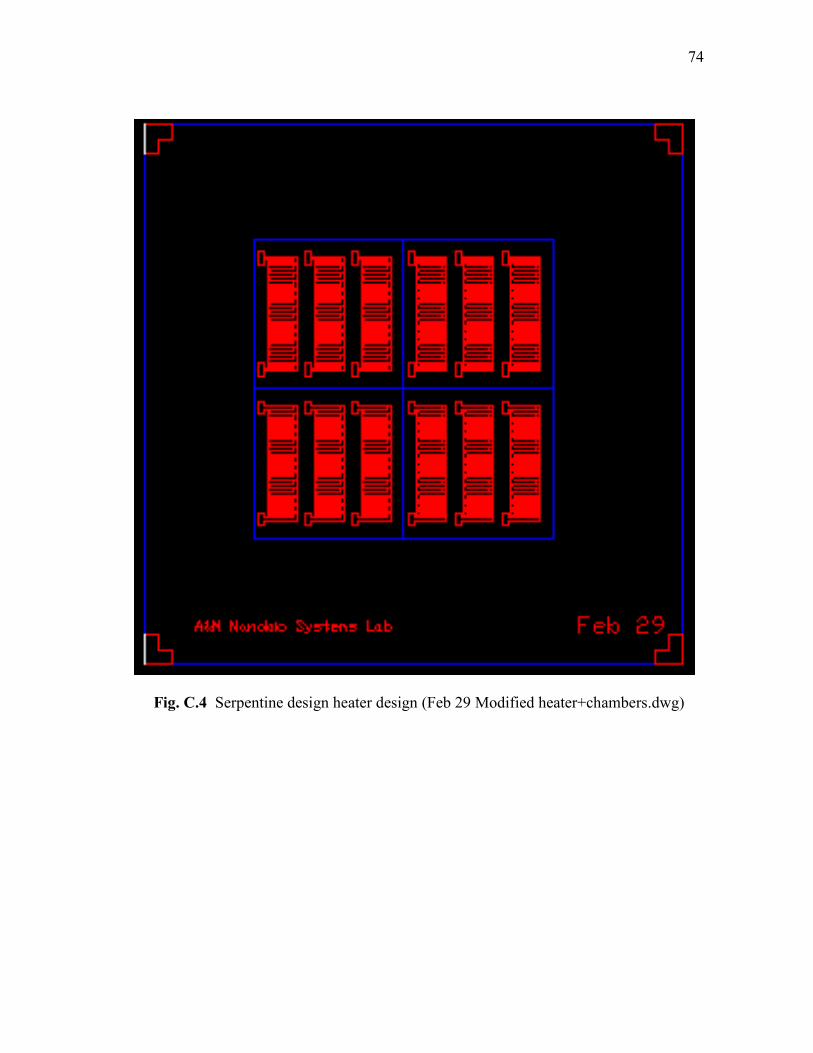
74
Fig. C.4 Serpentine design heater design (Feb 29 Modified heater+chambers.dwg)

75
APPENDIX D
MICROFABRICATION PROCEDURES
Microchamber Fabrication Procedure
1. Clean the 2-inch square glass slide using piranha solution (H2SO4:H2O2 = 3:1
(v/v)) for 20 minutes and then thoroughly rinse with deionized (DI) water and
dry with nitrogen gas.
2. Deposit Cr and Au layer using an E-beam evaporator to thickness of 180/1000
Angstrom.
3. Spin-coat photoresist (Microposit® S1818, Rohm-Haas-Shipley Company,
Inc., Marlborough, MA, USA) onto the wafer at 4000 rpm for 30 sec with an
acceleration of 5.
4. Soft bake the wafer at 110°C for 4 minutes.
5. Load the wafer to mask aligner (Karl Suss MA6 Mask Aligner, SUSS
Microtec, Inc., Waterbury Center, VT, USA) and expose to UV light for a
dose of 87 mJ/cm2.
6. Develop the photoresist using the developer (Microposit® MF-319, Rohm-
Haas14 Shipley Company, Inc., Marlborough, MA, USA) for about 1 minute.
7. Etch to the desired pattern using first gold and then chromium etchant.
8. Tape (MicroAmp® Optical Adhesive Covers, Applied Biosystems, Beverly,
MA, USA) the back side of the slide to avoid etching the back side of the
glass.

76
9. Prepare HF solution ((49%HF (J.T. Baker):H2O = 5:1 (v/v))) and etch the
glass for around 19 minutes to achieve 80 µm depth.
10. Remove the tape and etch the cover mask using gold and chromium etchant.
11. Cut the samples in four (There are four patterns in one glass slide) with
Professional Laser Series (PLS) 6.120D Laser Engraving and Cutting System
(Universal Laser Systems, Inc., Scottsdale, AZ, USA) using 50% power and
10% speed.
12. Drill the inlet and outlet holes using the drill. Before drilling, apply
CristalBondTM
509 (West Chester, PA, USA) wax to avoid cracks in the glass.
Heater Fabrication Procedure
1. Clean the 2-inch square glass slide using piranha solution (H2SO4:H2O2 = 3:1
(v/v)) for 20 minutes and then thoroughly rinse with deionized (DI) water and
dry with nitrogen gas.
2. Deposit Cr and Au layer using an E-beam evaporator to thickness of 200/2000
Angstrom.
3. Spin-coat photoresist (Microposit® S1818, Rohm-Haas-Shipley Company,
Inc., Marlborough, MA, USA) onto the wafer at 4000 rpm for 30 sec with an
acceleration of 5.
4. Soft bake the wafer at 110°C for 4 minutes.

77
5. Load the wafer to mask aligner (Karl Suss MA6 Mask Aligner, SUSS
Microtec, Inc., Waterbury Center, VT, USA) and expose to UV light for a
dose of 87 mJ/cm2.
6. Develop the photoresist using the developer (Microposit® MF-319, Rohm-
Haas14 Shipley Company, Inc., Marlborough, MA, USA) for about 1 minute.
7. Etch to the desired pattern using first gold and then chromium etchant.
8. Cut the samples in four (There are four patterns in one glass slide) with
Professional Laser Series (PLS) 6.120D Laser Engraving and Cutting System
(Universal Laser Systems, Inc., Scottsdale, AZ, USA) using 50% power and
10% speed

78
VITA
Osman Safa Cifci received his Bachelor of Science degree in Electrical
Engineering from Eskisehir Osmangazi University in 2009. He entered the Electrical
Engineering program at Texas A&M University in August 2010. His research interests
include miniaturization for life sciences applications.
Mr. Cifci may be reached at 214 Zachry Engineering Center TAMU 3128
College Station, TX 77843-3128. His email is [email protected].