Path Planning of Robots - Technical University of …etd.dtu.dk/thesis/258988/ep10_05.pdf · Path Planning of Robots Jan Holdgaard-Thomsen Kongens Lyngby 2010 IMM-M.Sc.-2010-5

Path Planning of Robots

Jan Holdgaard-Thomsen

Kongens Lyngby 2010IMM-M.Sc.-2010-5

Technical University of DenmarkInformatics and Mathematical ModellingBuilding 321, DK-2800 Kongens Lyngby, DenmarkPhone +45 45253351, Fax +45 [email protected]

IMM-M.Sc.-2010-5

Summary

Hospitals are ideal candidates for automation of transportation, as many itemsare transported daily from one location to another. The heavy load of trans-portation tasks requires a significant amount of manpower, and common tasksare mainly concerning transportation of trash, food, laundry, beds, samples,medical equipment, office supplies, mail etc.

In this thesis, the aim was to analyse this situation in a large, and with a focuson path planning as the central theme of this thesis. The thesis covers a numberof ways to characterize the path planning problem and the algorithms used toaddress it. The path planning strategy for a robot is a complex problem, itinvolves a wide range of subjects: complexity theory, mapping, path planningand more.

The presented strategies are evaluated based of the requirements for a hospitalenvironment like Bispebjerg Hospital. The thesis specifies the main problemsand challenges that need to be considered when designing such systems.

ii

Resume

Hospitaler er ideelle miljøer til automatisering af transportopgaver, mange tingtransporteres dagligt fra et sted til et andet. Den tunge belastning af trans-portopgaver kræver en betydelig mængde arbejdskraft; opgaverne handler hov-edsagelig om transport af skrald, mad, vasketøj, senge, prøver, medicinsk udstyr,kontorartikler, post osv.

I specialet var formalet at analysere denne situation i et større perspektiv, medfokus pa ruteplanlægning som det centrale tema. Specialet omfatter en rækkeforskellige mader at karakterisere ruteplanlægnings problemet og de algoritmer,der anvendes til at løse det. Ruteplanlægning for en robot er et komplekstproblem, der involverer en bred vifte af emner: kompleksitetsteori, kortlægning,ruteplanlægning mm.

De præsenterede strategier er vurderet pa grundlag af de krav som stilles til ethospitalmiljø som Bispebjerg Hospital. Specialet angiver de vigtigste problemerog udfordringer, som skal tages i betragtning ved udformningen af sadannesystemer.

iv

Preface

This thesis was prepared at the Department of Informatics and MathematicalModelling, the Technical University of Denmark in fulfilment of the requirementsfor acquiring the M.Sc. degree in engineering.

The thesis was written in the period from the 1th of September 2009 to the22th of February 2010. A current research project involving DTU Informatics,DTU Management, Force Technology, and Bispebjerg Hospital aims to reducethe required manpower by letting these transportation tasks be carried out bya mobile robot.

I would like to thank Thomas Bolander for consistently providing support andinput to the process while ensuring that I kept moving forward. I would alsolike to thank the individuals in the research project that have influenced thework.

I have written this thesis assuming that the reader comes with certain knowl-edge about algorithms in the field of path planning, and knowledge of basicmathematical concepts.

Lyngby, February 2010

Jan Holdgaard-Thomsen

vi

Contents

Summary i

Resume iii

Preface v

1 Introduction 11.1 Hospital Environment . . . . . . . . . . . . . . . . . . . . . . . . 21.2 Preconditions . . . . . . . . . . . . . . . . . . . . . . . . . . . . . 31.3 Computational Complexity . . . . . . . . . . . . . . . . . . . . . 5

2 Configuration Space 72.1 Robot Representation . . . . . . . . . . . . . . . . . . . . . . . . 82.2 Obstacle Representation . . . . . . . . . . . . . . . . . . . . . . . 9

3 Environment Representation 133.1 Topological Approach . . . . . . . . . . . . . . . . . . . . . . . . 143.2 Metric Approach . . . . . . . . . . . . . . . . . . . . . . . . . . . 153.3 Evaluation of Both Paradigms . . . . . . . . . . . . . . . . . . . . 15

4 Roadmaps 194.1 Visibility Graphs . . . . . . . . . . . . . . . . . . . . . . . . . . . 20

5 Cell Decompositions 23

6 Potential Field 29

7 Path Planning 357.1 Complete Motion Planning . . . . . . . . . . . . . . . . . . . . . 35

viii CONTENTS

7.2 A* Algorithm . . . . . . . . . . . . . . . . . . . . . . . . . . . . . 36

8 Carmen Robot Navigation Toolkit 398.1 Path Planning in Carmen . . . . . . . . . . . . . . . . . . . . . . 408.2 Evaluating Planning Approach in Carmen . . . . . . . . . . . . . 448.3 New Planning Approach in Carmen . . . . . . . . . . . . . . . . 45

9 Recommended approach for Bispebjerg 47

10 Conclusion 51

A map io.c 55

B test map.c 75

Chapter 1

Introduction

Automation techniques are applied widely in many fields like industrial plants,factories and offices. The main purpose of automation is both to save time andmanpower and to improve the service quality.

Hospitals are ideal candidates for automation of transportation, as many itemsare transported daily from one location to another by trained people. The heavyload of transportation tasks requires a significant amount of manpower, andcommon tasks are mainly concerning transportation of trash, food, laundry,beds, samples, medical equipment, office supplies, mail etc. This is not onlywaste of the trained personnels expertise but also a monotonous and tediouswork.

Automation is a key aspect for increasing efficiency and saving both time andmanpower. The main purpose of an automatic technology is to reduce theneed of human transportation tasks and replace them with robotic technologywhere the transportation task is suitable. A mobile robot that can performtransportation tasks could therefore relieve hospital personnel of this time con-suming, secondary task and free their time for the more critical primary duties

The solution will require an automation system consisting of a mobile robotthere is able to transport the different hospital equipment from one place toanother. The robot must be suitable for hospital environment where human

2 Introduction

traffic will not interfere with the system and not lead to potentially collisionswith people or interior. The system must therefore be able to deal with changesin its surrounding environments such as people and other obstacles.

One technology that has been successfully implemented in many industrial ap-plications to move materials around a manufacturing facility of a warehouse isAutomatic Guided Vehicle AGV. An AGV is a mobile robot which means therobot is not fixed to one physical location. The benefit of robotic technologyand the increasing knowledge from the research and the experience in indus-trial environments, result in introducing solutions to transportation of goods inplaces like hospitals. There exist several examples on utilizing robotic technol-ogy in hospitals. One of the earliest service robot projects is the HelpMate [19]robot capable of navigating hallways and riding elevators to deliver payloads toprogrammable destinations throughout a hospital. TUG [14] is another com-mercially available robot, which is able to transport attached wagons by tug-ging them. Another motivating example is the mobile robot named RHINO [15]which is a fully autonomous tour-guide at the Deutsches Museum Bonn. RHINOis able to lead museum visitors from one exhibit to the next by calculating apath using a stored map of the museum.

These examples indicate an increasing interest for such robotic systems. Theproject about implanting robots in a hospital was started by a Danish hospital,a company located in Copenhagen and Technical University of Denmark. Thisproject is concerning the sub problem of Path Planning this involves a numberof non-trivial subjects; this thesis will point out some of the important conceptsin path planning for mobile robots.

1.1 Hospital Environment

This section describes the environment of the hospital where the robot systemis to be implemented.

In order to identify the major problems it is necessary to analyse and examinethe needs of a transportation system. The case is Bispebjerg Hospital located inCopenhagen and consists of 51 buildings placed in a green oasis in the city. Thehospital has a capacity of approximately 500 beds and 3000 full time employees.Bispebjerg Hospital has gained status as a field hospital and the hospital isgradually growing to serve 400000 people. The hospital is built around theoriginal pavilions from 1913 and a few newer buildings, all connected throughan underground tunnel system. Today the majority of the transportation tasksuse the tunnel system. The tunnel network has a total length of 5 km, and the

1.2 Preconditions 3

longest distance from one point to another is 1.5 km. Elevators combined withthe tunnel system are suitable for transporting daily hospital equipment likebeds, garbage and food containers [29] (pp. 392-397). The environment at thehospital is rarely changing but furniture may be rearranged or hospitals bedsare placed in the hallway. And certain hallways are crowded at some specifictime of the day. To realize mobile service robots other requirements need tobe considered. They include ability to work without any adjustment to theenvironment for feasible implementation. To function in large scale workspacefor comprehensive working range.

1.1.1 Mobil Robot

The mobile robot technology provides a solution to the hospital transportationproblem. The mobile robot must be able to deal with changes in its surroundingenvironment; a mobile robot does not move along a fixed track and is thereforemore suitable for environments where humans are involved. The developmentof a mobile robot requires integration of capabilities, such as localization, map-ping, path planning, navigation, visual tracking, planning, signal processing andhuman robot interface etc. This project is avoiding reinventing what is madeavailable by others and focusing efforts towards new discoveries. Designing asoftware environment for robotic systems is not an easy task. Software develop-ment is a necessary process in autonomous mobile robotics and is becoming moreand more important to assist developers in their scientific and engineering work.Many existing programming environments, like The Player Project [45] (pages2421-2427), Carmen [23] (pp. 2436-2441), CLARaty [25] (pp. 2428-2435),OROCOS [28] (Vol. 14, pp. 33-49) and SmartSOFT [36] (pp. 253-263) are allproposing different approaches for Robotics Development Environments (RDE).Most of them are different in the use of specific communication protocols and/ormechanisms, different operating system, robotics platform, programming lan-guage etc. This project will not describe the different RDE since the RDE forthis project has been chosen to be Carmen [23] because it supports the hardwareof the mobile robot a Pioneer 3-AT from http://www.mobilerobots.com/.

1.2 Preconditions

This purpose of this section is to clarify the authors knowledge about the prob-lem, the decision of the mobile robot control software environment is alreadychosen to be Carmen [23]. This thesis will therefore not include an analysis andevaluation of various robotics software environments.

4 Introduction

1.2.1 Robotic Properties

In preparing of this thesis many properties of the robot are still unknown, ef-fective motion planning depends heavily on properties of the robot solving thetask. For example, if the robot is equipped with a car-like steering it can theo-retically reach any point and achieve any orientation within its two dimensionalenvironment, although it might have to carry out several and varied manoeu-vres to do so. This is due to the fact that this type of robot is only capableof executing a single displacement either forward or backward and a limitedsteering angle. This fact also means that this type of robot is capable of onlytwo controlled Degrees of Freedom (DOF) which is one fewer than are availablein its two dimensional environment. The robot is therefore non-holonomic. Ingeneral, a placement of a robot is specified by the number of parameters thatcorresponds to the number of DOF of the robot. This number is two for planarcar-like steering robots, and its three for planar robots that can rotate as well.The geometry of car-like is more complicated and since the properties of theactual robot are unknown I find it fair to restrict the robot of this thesis to beable to move in arbitrary directions. This thesis defines a method to representa robot by a point in a coordinate system, by definition this point is then calledthe reference point of the robot.

1.2.2 Requirements

Performance requirements for the robot are not yet decided, therefore, the cri-teria listed in this thesis are decided by the author. Since we deal with robotsthat carry out transport tasks, this thesis will mainly concentrate on completeplanners. Complete planning algorithms must find a path for the robot when-ever one exist and may only report failure if no path exist, but there is no claimsabout the quality of the path. The robot could make a large detour, or make lotsof unnecessary turns. In practical situations a good path is preferred not justany path. What constitutes a good path depends on the robot. In general, thelonger a path, the more time it will take the robot to reach its goal position. Fora mobile robot this means it can transport fewer goods per time unit, resultingin a loss of productivity. Therefore I will prefer a short path. Often there areother issues that play a role as well. For example, some robots can only move ina straight line; they have to slow down, stop, and rotate before they can moveinto different direction, so any turn along the path causes some delay. For thistype of robots not only the path length but also the number of turns along thepath has to be taken into account. In this thesis I ignore the aspect of the timeit takes the robot move along a specific path. When this thesis referees to theshortest path it means the Euclidean shortest path for a robot.

1.3 Computational Complexity 5

1.3 Computational Complexity

The objective of robot motion planning is to give the robot the capability ofplanning its own motion in an environment filled with obstacles. Path planningis a problem-solving competence, as the robot must decide what to do over thelong term to achieve its goal. Different types of motion planning problems maydiffer in their ”size” e.g. the dimension of the environment and the number ofobstacles. It is important to quantify the performance of the planning methods,typically the time required to solve the problem and the computational com-plexity of the planning problem. Analysis of the methods is useful to judge theirpracticality and to detect opportunities for improvements. The analysis of theproblem can also be useful to suggest new ways of formulating problems whenthe original formulation is too costly.

1.3.1 PSPACE-hard problem

This thesis will review an important theoretical result concerning the compu-tational complexity of robot motion planning. The problem was established byReif [31] for planning free paths in a configuration space of arbitrary dimension,often referred to as the ”Generalized Mover’s Problem” [31] or ”Piano Movers’Problem” [38].

Planning a free path for a robot made of an arbitrary number ofpolyhedral bodies connected together at some joint vertices, among afinite set of polyhedral obstacles, between any two given configura-tions, is a PSPACE-hard problem [20].

This regards the complexity of computational problems in terms of the amountof space, or memory, that they require. Time and space are two of the mostimportant considerations when seeking practical solutions to many computa-tional problems [42]. Explaining the definition of PSPACE will make use of theTuring machine model [42]. Turing machines are mathematically simple andclose enough to simulate real computers to give meaningful results. PSPACE isthe class of problems that are decidable in polynomial space on a deterministicTuring machine. Additional study on the exact path planning techniques for thegeneralized mover’s problem led Schwartz and Sharir [37] to an algorithm thatis expected to require at least exponential time on a nondeterministic Turingmachine, hence double exponential time on a deterministic Turing machine [20][10].

6 Introduction

The complexity of path planning described in the literature and in this sectiongives strong evidence that the time and space required to solve a motion planningproblem increases rapidly with the dimension of the environment. Therefore itis important to simplify the problem but still retain the problem realistically. Ifthe problem is reasonably well understood and if it is acceptable to trade somegenerality against better performance such a simplification is almost always fea-sible [20]. The simplification of the problem can be performed by the user orautomatically generated by an algorithm from the original input.

The following chapters present techniques for simplifying the motion planningproblem. Most of the discussion focuses on the robot representation, the rep-resentation of the environment and how to map the environment afterwardsits dealing with path planning in the representation. After that it is time toanalysis the methods used by Carmen and verify if Carmen is able to delivercomplete path planning and provide shortest path for a robot.

Chapter 2

Configuration Space

To create motion plans for robots, there is a need of specifying the dimensionsof the robot and obstacles in the environment. More specifically, there must begiven a specification of the location of every point on the robot and each obstacle,since the need of ensuring that no point on the robot collides with an obstacle.In this chapter the Configuration Space (C-space) [20] [10] is introduced.

The purpose is to give the robot the capability of planning its own motion,deciding automatically what motions to execute in order to achieve a task spec-ified by initial and goal position. Before the robot is able to plan a motion therobot must include knowledge about the environment in which it is moving. Forexample mobile robots moving around in hospitals must know where obstacleslike walls are located. The robot should be able to detect obstacles that are notincluded on the map like people moving around. For that information the robotwill have to rely on its sensors. Using information about the environment thebasic motion planning problem is defined as to produce a continuous motionin the C-space [20] [10] [11] connecting a start and a goal configuration whileavoiding obstacles in the environment.

The goal of defining a basic motion planning is to isolate some central issues andanalysis them in depth before considering additional difficulties. This sectionintroduces some of the basic notions used in motion planning. The generalmotion planning is complex task and there will be a number of simplifying

8 Configuration Space

assumptions.

2.1 Robot Representation

Let R be a robot moving around in a two dimensional environment. The envi-ronment will be a planar region with polygonal obstacles, since the actual sizeand shape of the robot in unknown I assume that R is a simple polygonal. Therobot motion depends on its mechanics. Some types of robots can move in anydirection, while others are limited motion. Robots with four wheels mountedlike a car cannot move sideways, and they often have a certain minimum turn-ing radius. Other robots can changes their orientation by rotation. C-spacedescribes the space of possible positions the robot may attain. For example in a2-dimensional environment a placement or configuration ofR can be specified bya translation vector. For instance, if the robot is a polygon with vertices (1,−1),(1, 1), (0, 3), (−1, 1) and (−1,−1), then the vertices of R (6, 4) are (7, 3), (7, 5),(6, 7), (5, 5) and (5, 3). With this notation, a robot can be specified by listingthe vertices of R.

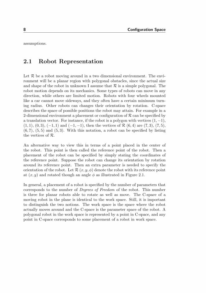
An alternative way to view this in terms of a point placed in the center ofthe robot. This point is then called the reference point of the robot. Then aplacement of the robot can be specified by simply stating the coordinates ofthe reference point. Suppose the robot can change its orientation by rotationaround its reference point. Then an extra parameter is needed to specify theorientation of the robot. Let R (x, y, φ) denote the robot with its reference pointat (x, y) and rotated though an angle φ as illustrated in Figure 2.1.

In general, a placement of a robot is specified by the number of parameters thatcorresponds to the number of Degrees of Freedom of the robot. This numberis three for planar robots able to rotate as well as move. The C-space of amoving robot in the plane is identical to the work space. Still, it is importantto distinguish the two notions. The work space is the space where the robotactually moves around and the C-space is the parameter space of the robot. Apolygonal robot in the work space is represented by a point in C-space, and anypoint in C-space corresponds to some placement of a robot in work space.

2.2 Obstacle Representation 9

Reference Point

R(0,0)

5

10

105

45o

R(6,4,45)

Figure 2.1: Describing the placement of a robot with three parameters, place-ment and rotation.

2.2 Obstacle Representation

It has now been described how to map placements of the robot to points in theC-space. The next thing to examine is how obstacles in the workspace can bemapped into the C-space for the robot. An obstacle P is mapped to the setof points p in C-space such that R(p) intersects P. Consider a circular mobilerobot in an environment with a single polygonal obstacle in the workspace, asshown in Figure 2.2. In Figure 2.2(b) the robot is moving around the obstacle


and keeping track of the curve traced out by the reference point. The referencepoint is chosen to be placed in the center of the robot, but could easily be placedat another position. Figure 2.2(c) shows the resulting obstacle in the C-space.Motion planning for a circular robot in Figure 2.2(a) is now equivalent to motionplanning for a point in the C-space, shown in Figure 2.2(c). Any open spacenot occupied by an object is free space, where the robot is free to move withouthitting anything modeled.

a b c

Figure 2.2: (a) The circular robot approaches the workspace obstacle. (b) Bymoving the robot around the obstacle the Configuration Obstacle Space (C-obs)is created. (c) Motion planning in the workspace representation (a) has beentransformed into motion planning in C-space.

The question that remains to be answered: is the robot colliding with an obstacleif it touches that obstacle? The obstacles can be defined to be topological openor closed [11]. Obstacles defined as open sets mean that the robot is allowed totouch them. In practice a movement where the robot passes very close to anobstacle cannot be considered safe because of possible errors in robot control.Such situations can be avoided by slightly enlarging all the obstacles beforecomputing a path.

The overall idea of configuration space formulation is to represent the robot asa point in the environment and to map the obstacles. The set of configurationsthat avoids collision with obstacles is called the Configuration Free Space (C-free). The complement of C-free in C-space is called the C-obs or forbiddenregion. It was recognized early on in motion planning research that the C-spaceis a useful way to abstract planning problems in a unified way. The advantageof this abstraction is that a robot with a complex geometric shape is mappedto a single point in the C-space. For path planning purposes the robot can bemodelled as a point as in Figure 2.2 so that the orientation is unimportant.This simplicity assumes the robot is holonomic, or can turn in place. Manyresearch robots are sufficiently close to be holonomic to meet this assumptionlike tour-guide robots that are able to interact and present exhibitions [40] [7]

2.2 Obstacle Representation 11

[27](pp. 95-124) [39](pp. 203-22).

The concept of metric path planning converts the representation of the environ-ment to a C-space representation that facilitates path planning. There exist alarge number of different C-space representations. The representations offer dif-ferent ways of partitioning free space. Any open space not occupied by an objectis free space, where the robot is free to move without hitting anything obstacles.Each partition can have additional information like ”this area is off-limit from9am to 5am,” etc.

The next step will be constructing a data structure for storing free space. Thisdata structure can then be used to compute a path between any two giveninitial and goal positions. This approach is useful when the work space is rarelychanged and many paths have to be computed. The possibilities to compute arepresentation of the free space will be discussed in the next chapter.


Chapter 3

Environment Representation

The environment representation can make a huge difference in the performanceand path quality. This chapter introduces and discusses the metric and topo-logical methods for building maps.

Building a representation of the environment is an important task for a mobilerobot that aims to move autonomously in the surrounding environment. Ifmany paths were to be planned in the same environment it would make senseto construct a data structure once and then use that data structure to plansubsequent paths more efficiently. This data structure is often called a map andmapping is the problem of exploring and sensing an unknown environment toconstruct a representation that is useful for navigation.

The literature of robotics describes two common paradigms for modelling indoorenvironments: metric or grid-based paradigm and topological paradigm [46].

14 Environment Representation

Center Left

Upper Left

Bottom Left Bottom Center

Center Center

Upper Center Upper Right

Center Right

Bottom Right

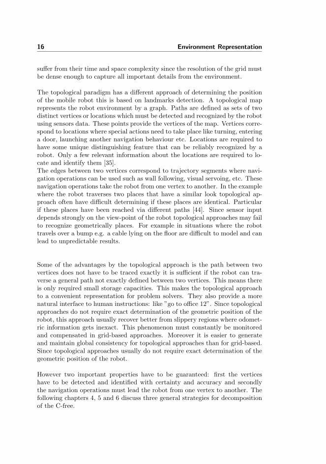
Figure 3.1: A real-world environment, areas shaded black represent obstacles inthe environment white areas represent free space.

3.1 Topological Approach

Upper Left

Center Left

Bottom LeftBottom Center

Center Center

Upper Left Upper Right

Center Right

Bottom Right

Figure 3.2: A topological map of the same area as Figure 3.1, with vertices rep-resenting places such as regions, and edges representing navigable paths betweenthese places.

Topological representations aim at representing environments with a graph struc-ture shown in Figure 3.2 where vertices correspond to distinct locations or land-marks. They are connected by an edge if there is a direct path between them.For example locations can be intersections and T-junctions in a building or anoffice. Figure 3.1 shows a real-world representation.

3.2 Metric Approach 15

3.2 Metric Approach

Figure 3.3: A metric map of Figure 3.1 with seven rooms connected by doors.Space is divided into equally sized squares with obstacles shaded black and freespaces blank.

A metric (grid-based) map represents environments by regular two dimensionalgrids shown in Figure3.3 and each grid cell may indicate the presence of anobstacle or free space in the corresponding region of the environment. In theserepresentations the environment is defined by a single global coordinate system,in which all mapping and navigation takes place. Regular grids are often referredto as occupancy grids [24].

3.3 Evaluation of Both Paradigms

Both approaches to mapping the environment either topological or metric havesignificant strengths and weaknesses. Metric maps are simple to construct andmaintain even in large-scale environments [6]. The grid-based approaches dis-tinguish between different places based on the geometric position within a globalcoordinate system. The position of the robot is estimated based on odometric in-formation and sensor readings from the robot. Thus occupancy grid approachesalso use a number of sensor readings to determine the location of the robot.To the extent that the position can be tracked accurately different positions forwhich sensor readings look alike are disambiguated by odometric information.Geometric locations are recognized as such even if the sensor readings are dif-ferent which is often the case in dynamic environments where movable interior,open doors or people can block the sensor of the robot. Grid-based approaches


suffer from their time and space complexity since the resolution of the grid mustbe dense enough to capture all important details from the environment.

The topological paradigm has a different approach of determining the positionof the mobile robot this is based on landmarks detection. A topological maprepresents the robot environment by a graph. Paths are defined as sets of twodistinct vertices or locations which must be detected and recognized by the robotusing sensors data. These points provide the vertices of the map. Vertices corre-spond to locations where special actions need to take place like turning, enteringa door, launching another navigation behaviour etc. Locations are required tohave some unique distinguishing feature that can be reliably recognized by arobot. Only a few relevant information about the locations are required to lo-cate and identify them [35].The edges between two vertices correspond to trajectory segments where navi-gation operations can be used such as wall following, visual servoing, etc. Thesenavigation operations take the robot from one vertex to another. In the examplewhere the robot traverses two places that have a similar look topological ap-proach often have difficult determining if these places are identical. Particularif these places have been reached via different paths [44]. Since sensor inputdepends strongly on the view-point of the robot topological approaches may failto recognize geometrically places. For example in situations where the robottravels over a bump e.g. a cable lying on the floor are difficult to model and canlead to unpredictable results.

Some of the advantages by the topological approach is the path between twovertices does not have to be traced exactly it is sufficient if the robot can tra-verse a general path not exactly defined between two vertices. This means thereis only required small storage capacities. This makes the topological approachto a convenient representation for problem solvers. They also provide a morenatural interface to human instructions: like ”go to office 12”. Since topologicalapproaches do not require exact determination of the geometric position of therobot, this approach usually recover better from slippery regions where odomet-ric information gets inexact. This phenomenon must constantly be monitoredand compensated in grid-based approaches. Moreover it is easier to generateand maintain global consistency for topological approaches than for grid-based.Since topological approaches usually do not require exact determination of thegeometric position of the robot.

However two important properties have to be guaranteed: first the verticeshave to be detected and identified with certainty and accuracy and secondlythe navigation operations must lead the robot from one vertex to another. Thefollowing chapters 4, 5 and 6 discuss three general strategies for decompositionof the C-free.

3.3 Evaluation of Both Paradigms 17

• Roadmap This approach is based on the following idea of capture theconnectivity of the robots C-free in the form of a network of one dimen-sional line segments lying in C-space. Once a roadmap is constructed theroadmap can be used as a set of paths. Path planning is then reducedto connect the initial and the goal state and searching the roadmap for apath [20]

• Cell Decomposition This approach is to decompose the C-free into acollection of non-overlapping regions called cells, whose union is exactlyC-free. Next thing is to construct a connectivity graph which representsthe adjacency relation among the cells which facilitates path searching. Ifsuccessful the output of the search is a sequence of cells often referred toas a channel [20], connecting the cells including the initial and the goalstate.

• Potential Field The two previous described methods aim at capturingthe connectivity of the C-free into a graph that is subsequently searchedfor a path. The potential field method is based on a different idea. Thisapproach creates a field or gradient across the C-free that directs the robotto the goal position from multiple prior positions.

The following sections present common instantiations of the road map, celldecomposition and potential fields. The sections introduce these approachesand illustrate them with simple examples in two-dimensional configuration spacepopulated by polygonal obstacles.


Chapter 4

Roadmaps

This section focuses on the class of topological maps called roadmaps. Theroadmap is a decomposition of the robot configuration space based specificallyon obstacle geometry. The challenge is to construct a set of paths that togetherenables the robot to go anywhere in its free space while minimizing the number oftotal roads. A roadmap is embedded in the free space and the vertices and edgesis included with physical meaning. Roadmap vertices correspond to a specificlocation and an edge correspond to a path between neighbouring locations. Theroadmap approach is based on the general idea of capture the connectivity ofthe robots C-free in the form of a network of one-dimensional lines that capturesthe topology of the free space [20]. Once a roadmap is constructed, it is usedas a network of road segments for robot motion planning. Robots make use ofroadmaps in much the same way as people use the highway system. Instead ofplanning every single street to a destination people normally plan their path to anetwork of highways, along the highway and finally from the highway system totheir destination. The key issue in this approach is obviously the construction ofthe roadmap. Various methods based on this general idea have been proposed.They compute different types of roadmaps called visibility graphs and Voronoidiagrams. In the case of visibility graphs roads become as close as possible to theobstacles and results in paths that are minimum-length solutions. Contrastingwith the visibility graph approach a Voronoi diagram is a complete roadmapmethod that tends to maximize the distance between the robot and obstacleson the map. Therefore the path in the Voronoi diagram is usually far from

20 Roadmaps

optimal in the sense of shortest path [40]. The Voronoi diagram method hasan important weakness in the case of limited range sensors. Since the methodmaximizes the distance between the robot and obstacles in the environment anyshort range sensor will have the risk of failing to sense its surroundings. Onthe other hand the visibility graph method can be designed to keep the robotas close as desired to obstacles therefore this thesis will only concentrate on thevisibility graph approach.

4.1 Visibility Graphs

The characteristics of a visibility graph are that its vertices share an edge ifthey are within line of sight of each other and that all points in the robots freespace are within line of sight of at least one vertex on the visibility graph [10] asshown in Figure 4.1. This method is one of the earliest path planning methods

Initial

Goal

Figure 4.1: The thin lines indicate the edges of the visibility graph of twoobstacles represented as filled polygons. The thick line represents the shortestpath between the initial and goal position.

and has been widely used to implement path planners for mobile robots [20].There are however two important cautions when using visibility graphs search:

• The size of the representation and the number of the edges and vertices in-creases with the number of obstacles polygons. This method can thereforebe slow and inefficient compared to other methods when used in environ-ments with a compact existence of obstacles. On the other hand can themethod be extremely fast and efficient in sparse environments.

4.1 Visibility Graphs 21

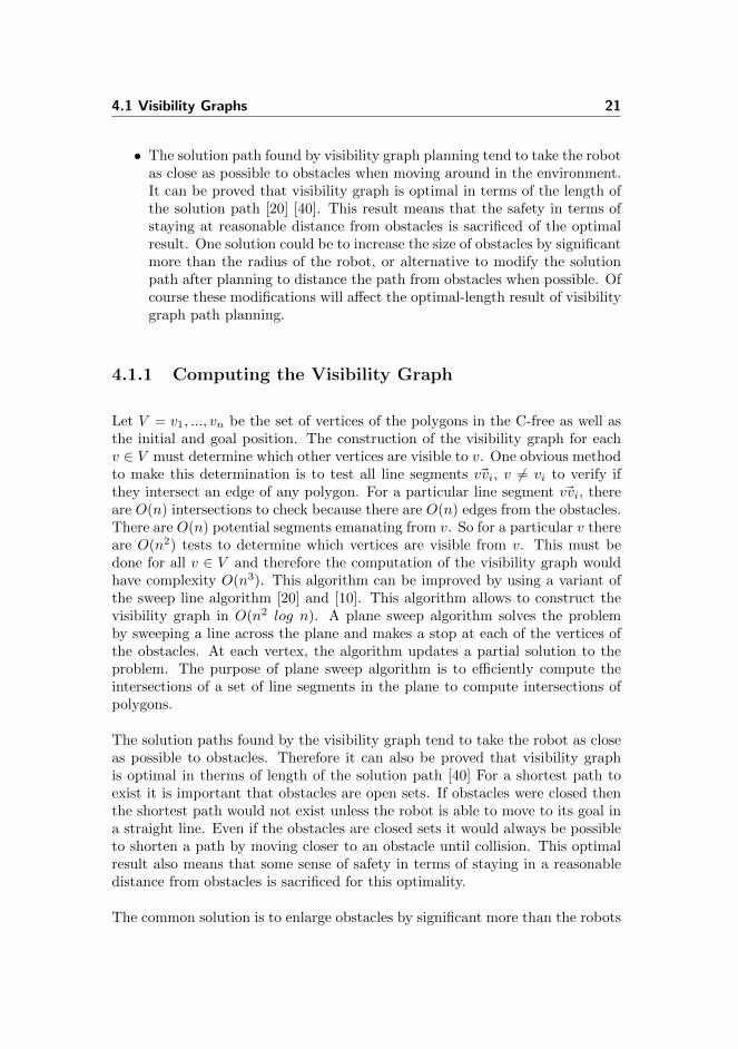
• The solution path found by visibility graph planning tend to take the robotas close as possible to obstacles when moving around in the environment.It can be proved that visibility graph is optimal in terms of the length ofthe solution path [20] [40]. This result means that the safety in terms ofstaying at reasonable distance from obstacles is sacrificed of the optimalresult. One solution could be to increase the size of obstacles by significantmore than the radius of the robot, or alternative to modify the solutionpath after planning to distance the path from obstacles when possible. Ofcourse these modifications will affect the optimal-length result of visibilitygraph path planning.

4.1.1 Computing the Visibility Graph

Let V = v1, ..., vn be the set of vertices of the polygons in the C-free as well asthe initial and goal position. The construction of the visibility graph for eachv ∈ V must determine which other vertices are visible to v. One obvious methodto make this determination is to test all line segments ~vvi, v 6= vi to verify ifthey intersect an edge of any polygon. For a particular line segment ~vvi, thereare O(n) intersections to check because there are O(n) edges from the obstacles.There are O(n) potential segments emanating from v. So for a particular v thereare O(n2) tests to determine which vertices are visible from v. This must bedone for all v ∈ V and therefore the computation of the visibility graph wouldhave complexity O(n3). This algorithm can be improved by using a variant ofthe sweep line algorithm [20] and [10]. This algorithm allows to construct thevisibility graph in O(n2 log n). A plane sweep algorithm solves the problemby sweeping a line across the plane and makes a stop at each of the vertices ofthe obstacles. At each vertex, the algorithm updates a partial solution to theproblem. The purpose of plane sweep algorithm is to efficiently compute theintersections of a set of line segments in the plane to compute intersections ofpolygons.

The solution paths found by the visibility graph tend to take the robot as closeas possible to obstacles. Therefore it can also be proved that visibility graphis optimal in therms of length of the solution path [40] For a shortest path toexist it is important that obstacles are open sets. If obstacles were closed thenthe shortest path would not exist unless the robot is able to move to its goal ina straight line. Even if the obstacles are closed sets it would always be possibleto shorten a path by moving closer to an obstacle until collision. This optimalresult also means that some sense of safety in terms of staying in a reasonabledistance from obstacles is sacrificed for this optimality.

The common solution is to enlarge obstacles by significant more than the robots

22 Roadmaps

radius, or alternative, to modify the path to distance from obstacles when pos-sible. Such actions sacrifice the optimal length results of visibility graph pathplanning.

Chapter 5

Cell Decompositions

The idea behind cell decomposition is to decomposing the C-free into simpleregions called cells. A non-directed graph represents the adjacency relation be-tween the cells. The shared boundaries of cells often have a physical meaningsuch as a change in the obstacle or a change in line of sight to surrounding.Two cells are adjacent if they share a common boundary a non-directed adja-cency graph encodes the adjacency relationships of the cells. From this grapha continuous path or channel can be determined by simply following adjacentfree cells from the initial point to the goal point. Cell decomposition methodscan be broken down into exact and approximate methods:

• Exact Cell Decomposition The first step in the method of cell de-composition is to decompose the C-free which is bounded both internallyand externally by polygons into trapezoidal and triangular cells by simplydrawing parallel line segments from each vertex of each interior polygonin the C-space to the exterior boundary. Then each cell is numbered andrepresented as a vertex in the adjacency graph. Vertices that are adjacentin the C-space are linked in the adjacency graph. A path in this graphcorresponds to a channel in free space which is illustrated by the sequenceof striped cells. This channel is then translated into a free path by con-necting the initial position to the goal position through the midpoints ofthe intersections of the adjacent cells in the channel.

24 Cell Decompositions

• Approximate Cell Decomposition This approach is different becauseit uses a recursive method to continue subdividing the cells until one ofthe following situations occurs. Each cell lies either completely in C-obsregion or completely in C-free. The other situation is when an arbitrarylimit in resolution is reached. Once a cell fulfils one of these criteria, itstops decomposing. In some literature this method is often called quadtreedecomposition because a cell is divided into four smaller cells of same shapeeach time its decomposed.

Both approaches for cell decomposition have advantages and disadvantages.Provided that each method is equipped with both appropriate search techniquesand exact computation techniques, exact cells decomposition method are com-plete meaning they are guaranteed to find a free path whenever one exists orreturn failure otherwise. Approximate methods may not be complete but theprecision of the approximation can be made arbitrarily small. However thetrade-off for this accuracy is a more complex mathematical process results in amore expense running time.

A B C D

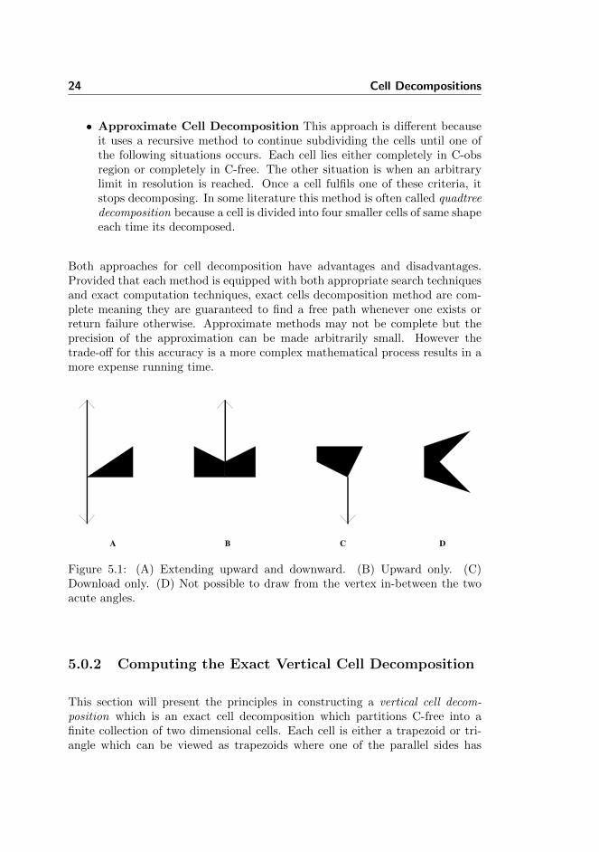
Figure 5.1: (A) Extending upward and downward. (B) Upward only. (C)Download only. (D) Not possible to draw from the vertex in-between the twoacute angles.

5.0.2 Computing the Exact Vertical Cell Decomposition

This section will present the principles in constructing a vertical cell decom-position which is an exact cell decomposition which partitions C-free into afinite collection of two dimensional cells. Each cell is either a trapezoid or tri-angle which can be viewed as trapezoids where one of the parallel sides has

25

a zero-length edge. For this reason this method is often called trapezoidal de-composition. The decomposition is defined as follows. Let P denote the set ofvertices used to define C-obs. At every p ∈ P draw a upward vertical lineand one downward vertical line through C-free through C-free until C-obs orthe boundary of C-space is reached. There are four possible cases, as shown inFigure 5.1 depending on whether or not it is possible to draw a line in the twodirections. If C-free is partitioned according to these rules, then the result is avertical decomposition of C-free shown in Figure 5.2. For simplicity assume that

Figure 5.2: The vertical decomposition method uses the cells to construct aroadmap, which is searched to yield a solution to a query.

each vertex on all of the polygons has a unique x-coordinate. A consequence ofthis is that there cannot be any vertical edges of C-obs. This assumption is notvery realistic. Vertical edges occur frequently in many environments and thesituation that two non-intersecting obstacles have an endpoint with the samex-coordinate is not unusual either because the precision or resolution (in whichthe coordinates are given) is often limited.

To deal with this problem a rotation of the axis-system could be a solution. If therotation angle is small enough then no two distinct will lie on the same verticalline any more. Rotations by very small angles however, lead to numerical diffi-culties. Even if the input coordinates are integer there is needed a significantlyhigher precision to perform the calculations properly. It will be convenient notto use rotation, but to use an affine mapping called shear transformation [30]Figure 5.3 illustrates the effect. The transformation in which all points alonga given line x-axis remain fixed while other points are shifted parallel to thex-axis, this transformation does not change the area of the environment [13].

For computing the decomposition the naive approach appears simple enoughthat all required steps can be computed by a brute-force algorithm. If C-obs


Figure 5.3: A transformation in which all points along a given line x-axis remainfixed while other points are shifted parallel to x-axis.

has n vertices then this approach would take at least O(n2) time because the in-tersection test has to be made between each vertical line and each obstacle. Thisrunning time can be improved and the resulting running time is only O(n log n)by making use of the line-sweep principle [5] [11]. This principle forms the basisof many combinatorial motion planning algorithms much of computational ge-ometry can be considered as the development of data structures and algorithmsthat generalize the sorting problem. In others words the algorithms carefully”sort” geometric informations [21]. In principle the algorithm sweeps a lineacross the plane only to stop where some critical change occurs in the infor-mation. To construct the vertical decomposition, imagine that a vertical linesweeps the plane from x = −n to x = n, using (x, y) to denote a point in theplane. Note that the only data that appears in the problem input is the verticesand edges of C-obs. It is therefore reasonable that interesting things can onlyhappen at these vertices. Sort the vertices in the input in increasing order bytheir x-coordinate. Assuming that not two vertices have the same x-coordinate.The vertices will now be visited in order of increasing x value. Each visit to avertex will be referred to as an event. Before after and in between every eventa list, L, of some C-obs edges will be maintained. This list must be maintainedat all times in the order that the edges appear when intersects by the verticalsweep line.

To be able to handle motion planning queries, a roadmap is constructed from thevertical cell decomposition as shown in Figure 5.4. For each cell Ci let pi denotea point such that pi ∈ Ci. The point can be selected as the geometric center.Let G(V,E) be a topological graph defined as follows. For each cell Ci define avertex pi ∈ V . There is a vertex for every line and for every cell. For each cell,define an edge from the cells geometric center to the center of every line that liesalong each cells boundaries. The resulting graph is a roadmap as in Figure 5.4.The accessibility condition from one point to another point is satisfied becauseevery point can be reached by a straight line path because of the convexity ofevery cell. Once the roadmap is constructed, the cell information is no longerneeded for answering planning queries.

27

Figure 5.4: The graph derived from the vertical cell decomposition.


Chapter 6

Potential Field

The potential field method treats the robot like a particle moving in a field underthe influence of an artificial potential field whose local variations are expectedto reflect the structure of the C-free. The robot then moves in the directionindicated by the potential field. The goal acts as an attractive force on the robotalso obstacles form a repulsive force directing the robot away from obstacles.The correct combination of repulsive and attractive forces moves robot from theinitial position to the goal position while avoiding obstacles. If new obstaclesappear during robot motion the potential field needs to be updated in order tointegrate this new information.

The drawback of the potential field method is that there is a tendency that therobot might get trapped in local minima which is not the goal position. Thiscan happen when the forces associated with the potentials evaluates to zeroand therefore the robot does not move. This happens in the situations wherethe attractive force towards the goal and the repulsive force are equal. As aresult the robot is trapped in local minima and in practice the robot oscillatesclose to the local minima. This means that there is no guarantee that potentialfield method will find a path to goal position. In Figure 6.1 the robot initiallyattracted to the goal as it approaches the horseshoe shaped obstacle. The goalis attracting the robot but the bottom of the obstacle repulses the robot upwarduntil the top of the horseshoe begins to influence the robot. At this point ithappens that the attractive force to the goal is symmetric to the repulsive force

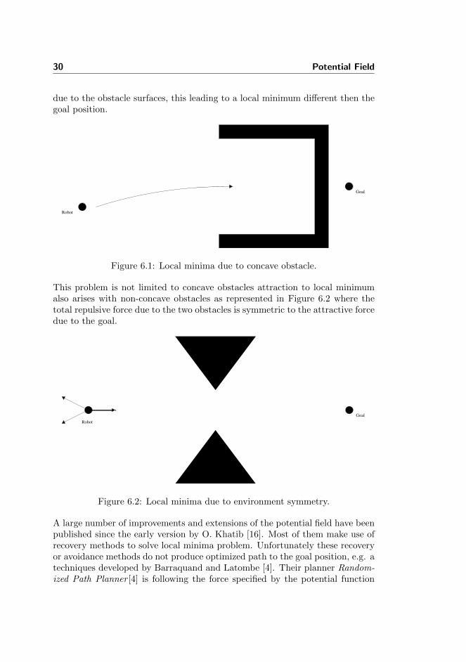
30 Potential Field

due to the obstacle surfaces, this leading to a local minimum different then thegoal position.

Goal

Robot

Figure 6.1: Local minima due to concave obstacle.

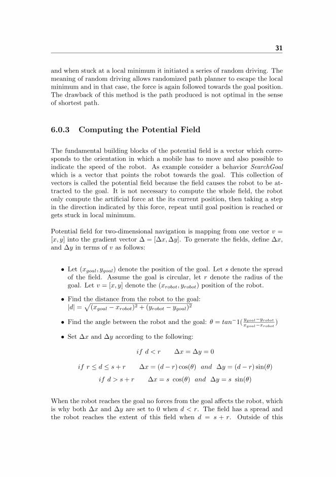
This problem is not limited to concave obstacles attraction to local minimumalso arises with non-concave obstacles as represented in Figure 6.2 where thetotal repulsive force due to the two obstacles is symmetric to the attractive forcedue to the goal.

Goal

Robot

Figure 6.2: Local minima due to environment symmetry.

A large number of improvements and extensions of the potential field have beenpublished since the early version by O. Khatib [16]. Most of them make use ofrecovery methods to solve local minima problem. Unfortunately these recoveryor avoidance methods do not produce optimized path to the goal position, e.g. atechniques developed by Barraquand and Latombe [4]. Their planner Random-ized Path Planner [4] is following the force specified by the potential function

31

and when stuck at a local minimum it initiated a series of random driving. Themeaning of random driving allows randomized path planner to escape the localminimum and in that case, the force is again followed towards the goal position.The drawback of this method is the path produced is not optimal in the senseof shortest path.

6.0.3 Computing the Potential Field

The fundamental building blocks of the potential field is a vector which corre-sponds to the orientation in which a mobile has to move and also possible toindicate the speed of the robot. As example consider a behavior SearchGoalwhich is a vector that points the robot towards the goal. This collection ofvectors is called the potential field because the field causes the robot to be at-tracted to the goal. It is not necessary to compute the whole field, the robotonly compute the artificial force at the its current position, then taking a stepin the direction indicated by this force, repeat until goal position is reached orgets stuck in local minimum.

Potential field for two-dimensional navigation is mapping from one vector v =[x, y] into the gradient vector ∆ = [∆x,∆y]. To generate the fields, define ∆x,and ∆y in terms of v as follows:

• Let (xgoal, ygoal) denote the position of the goal. Let s denote the spreadof the field. Assume the goal is circular, let r denote the radius of thegoal. Let v = [x, y] denote the (xrobot, yrobot) position of the robot.

• Find the distance from the robot to the goal:|d| =

√(xgoal − xrobot)2 + (yrobot − ygoal)2

• Find the angle between the robot and the goal: θ = tan−1(ygoal−yrobot

xgoal−xrobot)

• Set ∆x and ∆y according to the following:

if d < r ∆x = ∆y = 0

if r ≤ d ≤ s+ r ∆x = (d− r) cos(θ) and ∆y = (d− r) sin(θ)

if d > s+ r ∆x = s cos(θ) and ∆y = s sin(θ)

When the robot reaches the goal no forces from the goal affects the robot, whichis why both ∆x and ∆y are set to 0 when d < r. The field has a spread andthe robot reaches the extent of this field when d = s + r. Outside of this

32 Potential Field

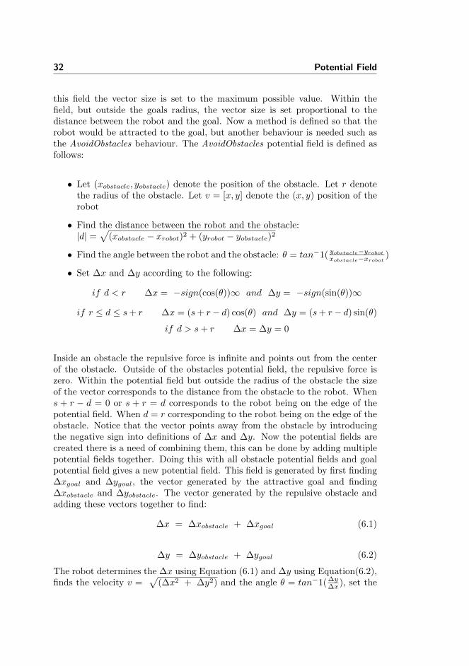
this field the vector size is set to the maximum possible value. Within thefield, but outside the goals radius, the vector size is set proportional to thedistance between the robot and the goal. Now a method is defined so that therobot would be attracted to the goal, but another behaviour is needed such asthe AvoidObstacles behaviour. The AvoidObstacles potential field is defined asfollows:

• Let (xobstacle, yobstacle) denote the position of the obstacle. Let r denotethe radius of the obstacle. Let v = [x, y] denote the (x, y) position of therobot

• Find the distance between the robot and the obstacle:|d| =

√(xobstacle − xrobot)2 + (yrobot − yobstacle)2

• Find the angle between the robot and the obstacle: θ = tan−1( yobstacle−yrobot

xobstacle−xrobot)

• Set ∆x and ∆y according to the following:

if d < r ∆x = −sign(cos(θ))∞ and ∆y = −sign(sin(θ))∞

if r ≤ d ≤ s+ r ∆x = (s+ r− d) cos(θ) and ∆y = (s+ r− d) sin(θ)

if d > s+ r ∆x = ∆y = 0

Inside an obstacle the repulsive force is infinite and points out from the centerof the obstacle. Outside of the obstacles potential field, the repulsive force iszero. Within the potential field but outside the radius of the obstacle the sizeof the vector corresponds to the distance from the obstacle to the robot. Whens + r − d = 0 or s + r = d corresponds to the robot being on the edge of thepotential field. When d = r corresponding to the robot being on the edge of theobstacle. Notice that the vector points away from the obstacle by introducingthe negative sign into definitions of ∆x and ∆y. Now the potential fields arecreated there is a need of combining them, this can be done by adding multiplepotential fields together. Doing this with all obstacle potential fields and goalpotential field gives a new potential field. This field is generated by first finding∆xgoal and ∆ygoal, the vector generated by the attractive goal and finding∆xobstacle and ∆yobstacle. The vector generated by the repulsive obstacle andadding these vectors together to find:

∆x = ∆xobstacle + ∆xgoal (6.1)

∆y = ∆yobstacle + ∆ygoal (6.2)

The robot determines the ∆x using Equation (6.1) and ∆y using Equation(6.2),finds the velocity v =

√(∆x2 + ∆y2) and the angle θ = tan−1( ∆y

∆x ), set the

33

speed to v and the direction to θ. as the robot moves in the environment it iden-tifies new force vectors, and chooses new directions and speed. The describedapproached is based on the following source [12], [34] and [33]

34 Potential Field

Chapter 7

Path Planning

In the previous chapters three methods for representing the environment hasbeen descried namely visibility graphs section 4.1, cell decomposition chapter 5and potential functions chapter 6. The two methods visibility graphs 4.1 and celldecomposition 5 approaches are complete which means that it is possible to finda solution if one exists otherwise they report failure. The third method potentialfunctions 6 is a heuristic method that is able to produce a fairly acceptablesolution to the problem in many scenarios, but for which there is no formalproof of its correctness.

7.1 Complete Motion Planning

To be able to provide complete motion planning the solution must adopt oneof the two following solutions visibility graphs 4.1 or cell decomposition 5 butto be able to provide the Euclidean shortest path the solution can only usevisibility graphs 4.1. The visibility graph of a set of non intersecting polygonalobstacles in the plane is an undirected graph whose vertices are the verticesof the obstacles and whose edges are pairs of vertices (u, v) such that the linesegment between u and v does not intersect any of the obstacles. Given thisgraph and two vertices initial and goal position the problem is now reduced to

36 Path Planning

generate a path such that the total path cost of the path is minimal among allpossible paths from initial to goal position. Any minimal cost path will do, andthe path should consist of a list of connections from the initial vertex to thegoal vertex. In many cases edges in graphs are labelled by cost and the cost ofa path is defined as the sum of the costs attached to its edge.

Various algorithms have been developed for planning paths. A selection of suchalgorithms is described in detail in various textbooks such as [26], [20], [11].Uninformed search methods are whether depth-first or breadth-first, methodsfor finding paths. In principle, these methods provide a solution to the path-finding problem, but they are often infeasible to use to control path findingsystems because the search expands too many vertexes before a path is found.The A∗ algorithm [26] [20] [10] is a classical and very well known algorithm. A∗is guaranteed to return a path of minimum cost wherever a path exists and toreturn failure otherwise under the specifications given here:

7.2 A* Algorithm

A∗ explores the graph G iterative by following paths originates from the initialvertex Vinit. In the beginning of each iteration there are vertices that the algo-rithm has already visited and there may be other vertices that are still unvisited.For each visited vertex V the previous iterations have produced one or severalpaths connecting Vinit to V the algorithm only stores a representation of a pathof minimum cost. At any instant the set of all such paths forms a spanning treeT of the subset of G so far explored. T is represented by associating to eachvisited vertex V a pointer to its parent vertex in the current T . A∗ assigns acost function f(V ) to every vertex in the current T . This function is an estimateof the cost of the minimum cost path in the graph G connecting Vinit to Vgoalgoing through N . The function f(V ) is computed as follows:

f(V ) = g(V ) + h(V ) (7.1)

where:

• g(V ) represents the true cost of the path from the initial vertex Vinit tothe current vertex V .

• h(V ) represents the estimated cost in moving from vertex V to the goalvertex Vgoal in G.

If this estimate is exactly equal to the distance along the optimal path theA∗ algorithm expands to very few vertices the reason is that A∗ is computing

7.2 A* Algorithm 37

f(V ) = g(V ) + h(V ) at every vertex. When h(V ) exactly matches g(V ) thevalue of f(V ) does not change along the path. All vertices that are not on theright path will have a higher value of f than vertices that are on the right path.Since A∗ does not consider higher valued f vertices until the algorithm hasconsidered lower valued f vertices the A∗ has a good possibility to not straysoff the shortest path.

7.2.1 Choosing an Estimate

The A∗ algorithm searches a graph efficiently, with respect to the chosen esti-mate; if the estimate is accurate then the search is efficient. If the estimate isinaccurate although a path will be found its search will take more time thanprobably required and possibly return a suboptimal path. If we are able tocompute a perfect estimate one that always returns the exact minimum pathdistance between two vertices the algorithm will perform efficient in O(n) wheren is the number of steps in the graph. The problem of calculating the exactdistance between two vertices is the same as finding the shortest path betweenthe two vertices - which is the problem we are trying to solve in the first place.For non perfect estimates A∗ behaves slightly differently depending on whetherthe estimate is too high or too low.

7.2.2 Underestimating

If the estimate is too low so that it underestimates the actual path length thealgorithm takes longer to run because A∗ will prefer to examine vertices closerto the start vertex, rather than vertices close to the goal. This will increase thetime it takes the algorithm to find the path through to the goal. If the estimateunderestimates in all possible cases then the result that the algorithm produceswill be the best path possible. If the estimates ever overestimates this guaranteeis lost. In applications where accuracy is more important than performance, it isimportant to ensure that the estimate is underestimating. In the majority of theliterature about path planning in commercial and academic problems, accuracyis often very important and therefore also the approach of underestimating [20][21] [22] [11].

38 Path Planning

7.2.3 Overestimating

If the estimate is too high so that it overestimating the actual path A∗ may notreturn the optimal path. A∗ will tend to generate a path with fewer vertices init, even if the edges between vertices are more costly to travel. The A∗ will payless attention to the cost so far travelled and will tend to favor vertices that haveless distance to travel. This will move the focus of the search toward the goalfaster but include the risk of missing a more efficient path. This means that thetotal length of the path may be longer than the most efficient path. This doesnot mean that an overestimated A∗ algorithm is producing poor paths, it canbe shown that if a estimate is overestimated by at most some value x for anyvertices in the graph, then the final path will be no more than x too long. Thisdoes not mean that the A∗ cannot be used with an overestimate, but it refersto the fact that the algorithm no longer returns the shortest path.

Most of the literature researched for this thesis aim for estimates that are close,but err on the side of underestimating. The simplest and most common estimateis Euclidean distance [22].

7.2.4 Euclidean Distance

A common estimate is the Euclidean distance which is guaranteed to be underes-timating [22]. The cost of an edge between two vertices is given by the distancebetween the representative vertices. The Euclidean distance is measured di-rectly between two vertices even if there is no direct path because of blockingobstacles. Euclidean distance is always either accurate or an underestimate.Moving around obstacles can only add extra distance. If there is no obstaclesbetween two vertices the estimate is accurate, otherwise it is an underestimate.

7.2.5 Summary

Until now the previous chapters has touched a number of ways to characterizethe motion planning problem and the algorithm used to address it. The mobilerobot control software environment is already chosen to be Carmen [23] thisthesis will therefore not include an analysis and evaluation of various roboticssoftware environments. Instead this thesis will focus on the methods used byCarmen to clarify if Carmen is able to deliver complete path planning andprovide the shortest path for a robot.

Chapter 8

Carmen Robot NavigationToolkit

Carmen [23] is an open source collection of robot control software developed in2002 by a group of people at Carnegie Mellon University in USA. Its mainlywritten in the C and C++ programming language, it consists of 640 files andmore than 111600 lines of code. It is developed to provide a ”consistent interfaceand a basic set of primitives for robotic research” [23] mainly focusing on singlerobot control. Carmen supports a large number of different robot platforms likeScout, XR4000, Segway and iRobot just to mention a few of the most famousplatforms. It uses a three layered architecture; the first layer is the hardwareinterface providing low-level control integration of sensor and motion data, thesecond layer is concerning all basis robot tasks such as motion planning, obstacleavoidance and localization etc. and the third layer is the user-defined applica-tion which relies on the functionality of the lower levels. Carmen also providesa configuration tools, a simulator and a map editor tool. Carmen was designedas modular software architecture, with each major capability built as a separatemodule. Modules communicate with each other over a communication protocolcalled Inter Process Communication (IPC) [8] which provides message passingbetween processes. Carmen supports autonomous mobile robot navigation inindoor environments. It contains software modules for collision avoidance, lo-calization, mapping, path planning, navigation and people tracking [23].

40 Carmen Robot Navigation Toolkit

8.0.6 Map Files

The essence of the Carmen navigation routines are based on metric environ-ment maps Figure 8.1 depict such a map file. This map file is a real worldexample taken from a senior care center in Pittsburgh; the map is included inCarmen software package. Map files in Carmen stores an evidence grid repre-sentation of two dimensional environment as well as other information relatedto robot navigation and localization. The evidence grid approach represents therobots environment by a two dimensional regular grid. In each cell is storedthe evidence or probability based on accumulated sensor readings that describea particular grid cells accessibility. In modern literature this approach is oftenreferred to as the occupancy grid where each cell holds a probability value thatindicates if the cell is either occupied, free or undiscovered. Occupancy gridswere first defined by Hans Moravec and Alberto Elfes [24].

Figure 8.1: Carmen map file of from the Long Wood senior care center

8.1 Path Planning in Carmen

The author Kurt Konolige is making the statement in article [18] that the de-scribed method unlike potential field methods in general, have the characteristic

8.1 Path Planning in Carmen 41

that it is impossible to get stuck in a local minimum. Since local minimum otherthan the goal position are major cause of inefficiency for potential field methods,an important question is the following: Is it possible to construct a potentialfunction which only has one local minimum a goal position. Such a function, ifit exists is called a ”global navigation function”

Computing local-minima-free potentials in large dimensional spacesis a difficult problem that is at least as hard as path planning it-self [17].

In chapter 8 it has been described how to construct a navigation function, i.e.a potential field. To construct the potential field with no local minimum otherthan the goal configuration is a difficult problem that has a known solutiononly when the C-obs have simple shapes [20]. The computation of a numericalnavigation function over a representation of the C-space in form of a grid turnsout to be a easier problem. That is probably the main reasons why Carmen isusing a grid approach, since it is difficult to construct an navigation functionover a C-free of arbitrary geometry.

According to the article [23] the current path planning implementation in Car-men is an implementation of Konoliges Linear Programming Navigation gradientmethod or LPN [18]. This section is describing the method presented in [18]the LPN gradient method is based on a numerical artificial potential field asdescribed in chapter 6. The article shows how to build a navigation functionthat assigns a potential field value to every point in the space. Moving along thegradient of the navigation potential yields the minimum cost path to the goalset. The method samples the C-space and assumes that C-space is to be dis-cretized into a set of points. Values at non-sampled points are being computedby interpolation between sample points.

8.1.1 Path Cost

The purpose is the find a path with minimum cost to some goal point. A pathis represented by an ordered set (8.1) of sampling points.

P = p1, p2, p3, ... pn (8.1)

Where the points are contiguous in either rectilinearly or diagonally and nopoints are repeated and the last point in the set must be the goal point. A costfunction F (P ) for a path P can be divided into the sum of a cost of being at a


point, along with an adjacency cost of moving from one point to the next one.

F (Pk) =∑i

I(pi) +∑i

A(pi, pi+1) (8.2)

Where A and I can be arbitrary functions. I will represent the cost of traversingthrough a given point, and will be set according to how close the robot is tooobstacles or have higher value for unknown regions, slippery regions, etc. WhileA is proportional to the Euclidean distance between two points, then the sumof A gives a cost proportional to the path length.

8.1.2 Navigation Function

A navigation function is the assignment of a potential field value to every point ofthe C-space, such that the goal point is always attracting the robot everywhere inthe environment. Navigation functions unlike potential field methods in generalhave the characteristic that it is impossible to get stuck in a local minimum [18].The value of the navigation function Nk in a point pk is the cost of the minimumcost path that starts from that point.

Nk = minj=1, ... ,m F (P jk ) (8.3)

Where P jk is the j-th path starting from point pk and reaching the goal set point

and m is the number of such paths. Calculating the navigation function Nk (8.3)for every point in the C-space directly, would require a very high computationaltime. Since the size of the C-space can be large, and finding the minimal costpath in a naive manner involves iteration over all paths from the point.

The LPN algorithm [18] is used to efficiently compute the navigation function.It is a generalization of the wavefront algorithm [43] [1] the algorithm is basedon the following three steps:

• Assign all goal set points a value 0, and every other point an infinite cost

• Put the goal set point in an active list

• At each iteration of the algorithm, operate on each point of the active list,removing it from the list and updating its eight neighbours

Consider an arbitrary point p that have assigned a value this point is surroundedby eight neighbours on a regular grid as in Figure 8.2. The process is repeateduntil the active list is empty. To update a point p are the following operationsused:

8.1 Path Planning in Carmen 43

• For every point q in the eight neighbours of p compute its cost to extendthe path from p to this point and the intrinsic cost of q using Equation (8.2)

• If the new value for q is less than the previous one, update the value for qand put it into the active list

The navigation function is computed according to the intrinsic cost of the sam-pling points in the C-space.

I = 5

q

p

C = 20

C old = 40 C new = 39

A = 14

Figure 8.2: Updating the cost of points in the neighbourhood of an active point.

8.1.3 Obstacle Cost

Suppose obstacles in the environment are given by a set of obstacle samplingpoints. Let Q be a generic function and d(p) the Euclidean distance for thesampling point p from the closest sample point representing an obstacle then:

I(p) = Q(d(p)) (8.4)

In order to compute d(p) for every sampling point involves the LPN algorithm bygiving the obstacle sampling points as the final configuration set, and assigningin the initialization phase a value 0 to the intrinsic cost for all the sampling


points. Once d(p) and then I(p) is computed for every sampling point p theLPN algorithm can again be executed to compute the navigation function.

8.2 Evaluating Planning Approach in Carmen

The article [18] referred in this section describing the gradient method a methodfor local navigation. Potential field methods are often referred to as local meth-ods. This comes from the fact that most potential functions are defined in sucha way that their values at any configuration do not depend on the distributionand shapes of the C-obs beyond some limited neighbourhood. If however itcould be possible to construct an ”ideal” potential function with a single min-imum at the goal position. This function could be regarded as some kind of”global” information about the C-free, and the expression ”local” would thenbe less relevant[20].

Most planning methods based on potential field approach like the one used inCarmen are incomplete, they may fail to find a free path, even if one exists.[20].On the other hand they are particular fast in a wide range of situations. Thestrength of this approach is that, with some engineering like the ”random driv-ing” approaches it makes it possible to construct motion planners which are bothquite efficient and reasonably reliable. This explains why they are increasinglypopular for implementing practical motion planners.

The potential field planner has successfully solved difficult problems [3] [9].However it is easy to create problems that it fails to solve in a reasonable amountof time, though they admit rather obvious solutions [2]. Most failures are causedby local minimum the problem is that it is difficult in general to ensure thatthe potential function will not contain multiple local minima. The robot couldbecome trapped at a local minimum that is not a goal position. In the researchfor this thesis I identified four significant problems; the problems are based onexperimental work with Carmen and problems described in the literature.

• Trap situations due to local minimum

• No passage between closely spaced obstacles

• Oscillations in a narrow passage

• Oscillations in the presence of obstacles

8.3 New Planning Approach in Carmen 45

8.3 New Planning Approach in Carmen

The problems encountered with the potential field and thereby with Carmenare leading to develop another planner. The planner in Carmen is a heuristicmethod, in the new planning approach the requirement from the section 1.2 acomplete planner. To develop a new planning approach in Carmen one of thefirst steps is to analysis the map files to verify is the map files include suitabledata to develop a new planner. The map files in Carmen stores a occupancygrid representation of two dimensional environment as well as other informationrelated to robot navigation and localization. The format of these map files isa tagged file format, similar to the TIFF standard for image files. The mapfile begins with an arbitrary number of lines all starting with ], these linesare comments. The documentation of Carmen is very limited though is theofficial description of the Carmen map file format available on the web page forCarmen [41].

To be able to read the information stored inside the map files, if a new planningapproach is needed I need to be able to read the map files. To be able to dothat I need to figure out how Carmen itself reads the map files. Carmen is usinga library file for reading the maps, it is located at /carmen/lib/libmap io.a.Then apply to the following function carmen map read gridmap chunk() in filemap io.c:

1 int carmen map read gridmap chunk (char ∗ f i l ename , carmen map t∗map) ;

When the function carmen map read gridmap chunk() is evoked including anappropriate map variable, it is filled with data from the map. The map variableshould be a pointer to a carmen map t structure:

1 typedef struct {2 carmen map conf ig t c on f i g ;3 f loat ∗ complete map ;4 f loat ∗∗ map ;5 } carmen map t , ∗carmen map p ;

The config substructure is defined as:

1 typedef struct {2 int x s i z e ;3 int y s i z e ;4 double r e s o l u t i o n ;5 char ∗map name ;6 } carmen map conf ig t , ∗ carmen map conf ig p ;

The map representation is a two dimensional array in [x], [y] it describes the


occupancy values at each grid cell. Values between 0.00 and 0.99 are free inthe sense of its value. 1.00 corresponds to occupied grid cells and the value −1is unexplored grid cells and is treated as occupied grid cells. The output fromrunning the readmap application:

1 jht@jht :˜/01 readmap/ readmap reviewed . / test map longwood .map2 Map in longwood .map i s 536 x 379 , with r e s o l u t i o n 0 .10 x 0 .10

m/ gr id c e l l3 The p i x e l at the cent r e o f the map i s 268 , 189 and has value 0 .274 The t o t a l gr id−po in t s in longwood .map i s : 203144

The result of running the readmap application on the map file longwood.map

provides the following information, the resolution is 0.10 x 0.10 m a preciseposition of the obstacles in the map is not given, only a value 1.00 for a solidobstacle. Since the resolution is 0.10 x 0.10 m we can only be sure to determinethe placement of obstacles within a margin error of 0.10 m. This is not preciseenough to continue implementing an exact shortest path approach, since therobot in these methods is moving very close to the obstacles in the environment.

The maps and code are based on a software package Carmen, the source filesmap io.c and test map.c can be found in the appendix.

Chapter 9

Recommended approach forBispebjerg

When evaluating the techniques described in this thesis it is important to alsopay attention to the environment Bispebjerg Hospital where the robot has tooperate. This chapter will sum up the advantages and disadvantages of metricand topological approach to mapping in the Table 9.1 and based on the descrip-tion from section 1.1 this section will try to create an idea of the best suitedapproach for the environment at Bispebjerg Hospital. A map of the tunnelsystem can be seen in the Figure 9.1. The tunnel system is a fairly simple struc-ture, if the cargo its not life-threatening material we will properly been satisfiedwith a suboptimal path and the effort in finding the precise shortest path is lessimportant. In the tunnel environment many hallways and corners may look thesame, and with the topological approach it can be hard to distinguish betweendifferent places. The robot can easily mistake one position for the other. Thesetwo reasons indicate that a metric approach will be the preferred method to thisspecific hospital environment. A following test drive either in the real environ-ment with a physical robot or a simulation in the map of the tunnel system willindicate the risk of ending up in a local minimum.

Other articles are proponent for an approach that integrates both paradigms:metric and topological, by combining both paradigms the approach presented inthis article [44] claims that it gains advantages from both worlds accuracy and

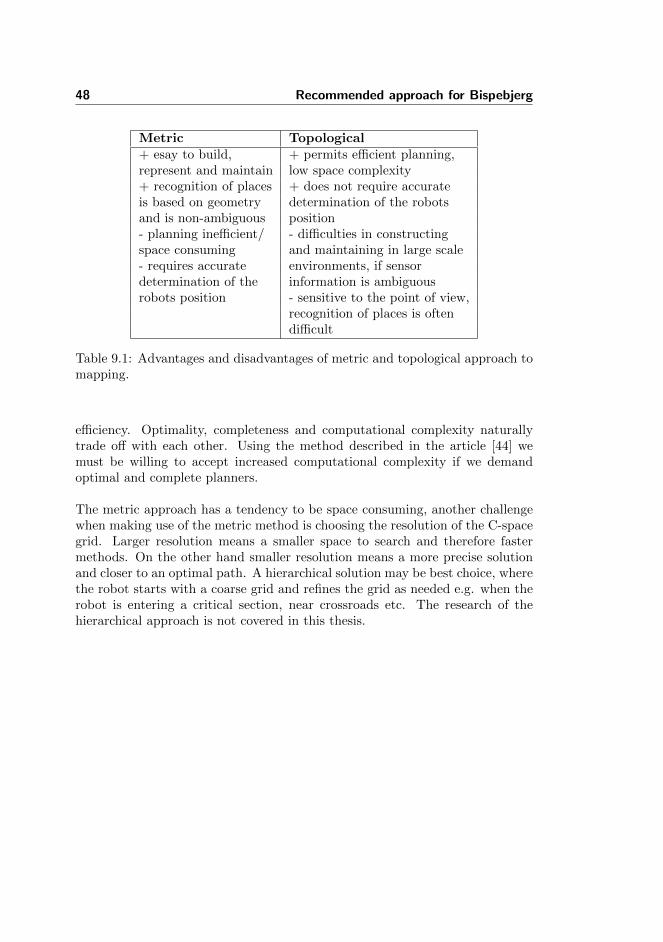
48 Recommended approach for Bispebjerg

Metric Topological+ esay to build, + permits efficient planning,represent and maintain low space complexity+ recognition of places + does not require accurateis based on geometry determination of the robotsand is non-ambiguous position- planning inefficient/ - difficulties in constructingspace consuming and maintaining in large scale- requires accurate environments, if sensordetermination of the information is ambiguousrobots position - sensitive to the point of view,

recognition of places is oftendifficult

Table 9.1: Advantages and disadvantages of metric and topological approach tomapping.

efficiency. Optimality, completeness and computational complexity naturallytrade off with each other. Using the method described in the article [44] wemust be willing to accept increased computational complexity if we demandoptimal and complete planners.

The metric approach has a tendency to be space consuming, another challengewhen making use of the metric method is choosing the resolution of the C-spacegrid. Larger resolution means a smaller space to search and therefore fastermethods. On the other hand smaller resolution means a more precise solutionand closer to an optimal path. A hierarchical solution may be best choice, wherethe robot starts with a coarse grid and refines the grid as needed e.g. when therobot is entering a critical section, near crossroads etc. The research of thehierarchical approach is not covered in this thesis.

49

Figure 9.1: The black solid lines illustrates the tunnel system of BispebjergHospital.

50 Recommended approach for Bispebjerg

Chapter 10

Conclusion

In this thesis I have examined the possibilities of creating a robotic transporta-tion system to solve logistic tasks in a hospital environment. Since approxi-mately 83 percent of hospital budgets are salaries, an automation of logisticstasks will reduce the need of human transportation tasks and release hands forbetter patient care by the increasing volume of patients with no correspondingincrease in staff [32]. The overall goal is to create autonomous robots that willaccept high-level descriptions of tasks and will execute them without furtherhuman intervention. The input description will specify what the user wantsdone rather than how to do it. Making progress toward autonomous robots isa practical interest not only in a hospital environment but in a wide variety ofapplication domains includes construction, assistance for the disabled, manu-facturing, and space exploration.

It is also of great technical interest, especially for Computer Science because itraises many important problems. One of them is path planning which is thecentral theme of this thesis. The minimum to expect from an autonomous robotis the ability to plan its own motion. At the first impression of motion planningit can look relatively simple, since people deal with it with no apparent diffi-culty in their everyday lives; it turns out to be extremely difficult to duplicatethis behaviour using a computer controlled robot. The unaware reader will besurprised by the amount of non-trivial mathematical and algorithmic techniques

52 Conclusion

that are necessary to build a reasonably general and reliable path planner.

This thesis introduces the concept of configuration space it is used throughoutthis thesis in order to organize the various aspects of motion planning. Theconcept is essentially a representational tool, it consists of treating the robot asa point in an appropriate space. Various tools from Geometry, Topology andAlgebra apply nicely to this representation and provide the theoretical basicof path planning. Chapter 2 describes the notation of the configuration spacefor a rigid object that can move and rotate freely among obstacles in a two di-mensional environment, the type of robot considered in the basic path planningproblem. The chapter also describes how the obstacles contained in the envi-ronment are mapped into the configuration space. The concept of configurationspace is a tool for formulating path planning problems precisely. In chapter 3two paradigms for mapping indoor environments are discussed, many factorsneed to be observed and evaluated to decide what type of approach to use.These include ease of construction, type of environment, storage requirements,equipment availability/cost, processing power requirement and suitability to thetask. Metric maps which stores information regarding to the obstacles in theenvironment are relative easy to construct but need large amount of storageand can be computationally complex due to the number of grid cells. Topo-logical maps are abstract representations of metric maps; topological maps aregenerated by partitioning the grid-based map into recognizable regions. Thetopological map is consistent with the grid-based map. For every abstract plangenerated using the topological map, there exists a corresponding plan in thegrid-based map. Typically, when using abstract models efficiency is traded offwith consistency and performance loss.

Chapter 4, 5 and 6 describe three computational approaches for solving thebasic path planning problem. Chapter 4 presents a roadmap approach calledvisibility graph, which consists of capturing the global topology of the set ofcollision free paths for the robot in form of a graph structure. Chapter 5 de-scribes the cell decomposition approach, which represents the set of collisionfree configurations as a collection of cells and search the graph representing theadjacency relation among these cells. Chapter 6 describes the potential fieldapproach, where the robot reacts as a particle moving under the action of forcesgenerated by an artificial potential field attracting the robot toward the goalwhile a repulsing force directing the robot away from obstacles. The roadmapand cell decomposition methods reduce the problem of finding a continuous freepath to that of searching a graph.

Chapter 7 introduces path finding with the A∗ algorithm. A∗ is a very efficient

53

algorithm and has lots of scope for optimization, many path finding systemsare using some variation of the A∗ as its key algorithm [22]. The property ofthe robot is highly dependent of the choice of the best suited approach, suchas wheel settings, turning radius and the dimensions of the robot etc. If therobot is installed with precise hardware for measuring odometric then a metricapproach could be the best approach. On the other hand if the money is spendon optimal sensors able to distinguish and detect landmarks in the hospital en-vironment, then the topological approach could be a better approach. Againthe best approach depends heavily on the robot and the hardware installed onthe robot.

The vast majority of the articles which I have studied during the preparationof this thesis has built a robot which is able to perform a given task like thetour-guide robot RHINO [6]. Based on the choice of hardware installed onthe robot, task specification, the environment and basic requirements, after allthese issues has been decided or analysed the choice of path planning approachcan begin. Developing the technologies required for autonomous robots are amajor challenge which involve many important problems, we see that many mo-bile robot applications are being built from scratch including the RHINO [6],HELPMATE [19] and TUG [14], this makes the automation process relativeexpensive. Research is needed in this area to find general solutions and to findrobust, reliable and safe methods and algorithms.

Carmen is one approach for providing robot motion control but is limited to thepotential field method; this technique has a limited ability to deal with localminima of the potential field function. The method is usually incomplete i.e. itmay fail to find a free path, even if one exists. The advantage is that in a widerange of situations some of them are particularly fast. After installing Carmenand simply setting up different path planning task for the robot simulator inCarmen, it is obvious that Carmen has problems. The robot has a tendencyto get trapped in complex concavities formed by a collection of obstacles; thecombination can act as a local minimum. Typically these trapped situationsare caused by the fact that the various points which have fixed positions areconcurrently attracted toward their goal position. Hence they are competingamong themselves to attain their goal positions. To prevent this problem onecan design a potential field that has no local minimum other than the goalconfiguration in the C-free. Another approach is to complement the potentialfield method with mechanisms for escaping local minimum; this could be one ofthe following approaches:

• Backtrack when encountering local minimum

54 Conclusion

• Take a number of random walks when encountering local minimum

• Invoke an alternative planner, such as a wall follower

• Increase the potential of obstacles, so that the robot is repulsed from thelocal minima

There are benefits of using the potential fields:

• Paths do not need to be planned, but are generated in real time

• Planning and control are merged in one function

• Paths are smooth, the robot does not brush along obstacles.

• Potential field can be dynamically updated

• To speed up computation, only local obstacles can be taken into account

When using the potential field method the effort must be put in developinga method for avoiding local minimum or escape from local minimum. Theconcept of the precise ”shortest path” in terms of distance is given up since therobot is not moving close to the obstacles. A shortest path would not exist interms of distance, as it will always be possible to shorten a path by movingcloser to obstacles. Also the concept of ”complete planner” is given up, sincethe potential field is a local method, at each step they move from one gridconfiguration to another. It is typical for this method to depend only on thecontent of the C-space in the neighbourhood of the current configuration ofthe robot. Therefore potential field methods are often called local methods,while the roadmap and cell decomposition methods are called global methods.We must be willing to accept increased computation complexity if we demandoptimal motion plans or completeness from our planner. One could argue that”shortest path” and ”complete planner” are not important in the robotic projectat Bispebjerg Hospital; if that is the case then the potential field method couldbe the best approach.

There are a number of interesting path planning concepts not covered in detailin this thesis, such as navigation among moving obstacles and coordination ofmultiple robots.

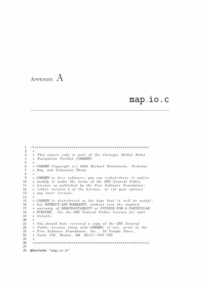
Appendix A

map io.c

1 /∗ ∗∗∗∗∗∗∗∗∗∗∗∗∗∗∗∗∗∗∗∗∗∗∗∗∗∗∗∗∗∗∗∗∗∗∗∗∗∗∗∗∗∗∗∗∗∗∗∗∗∗∗∗∗∗∗∗2 ∗3 ∗ This source code i s par t o f the Carnegie Mellon Robot4 ∗ Navigat ion Too l k i t (CARMEN)5 ∗6 ∗ CARMEN Copyright ( c ) 2002 Michael Montemerlo , Nicho las7 ∗ Roy , and Sebas t ian Thrun8 ∗9 ∗ CARMEN i s f r e e so f tware ; you can r e d i s t r i b u t e i t and/or

10 ∗ modify i t under the terms o f the GNU General Pub l i c11 ∗ License as pub l i s h ed by the Free Software Foundation ;12 ∗ e i t h e r ver s ion 2 o f the License , or ( at your opt ion )13 ∗ any l a t e r ver s ion .14 ∗15 ∗ CARMEN i s d i s t r i b u t e d in the hope t ha t i t w i l l be use fu l ,16 ∗ but WITHOUT ANY WARRANTY; wi thout even the imp l i ed17 ∗ warranty o f MERCHANTABILITY or FITNESS FOR A PARTICULAR18 ∗ PURPOSE. See the GNU General Pub l i c License f o r more19 ∗ d e t a i l s .20 ∗21 ∗ You shou ld have rece i v ed a copy o f the GNU General22 ∗ Pub l i c License a long with CARMEN; i f not , wr i t e to the23 ∗ Free Software Foundation , Inc . , 59 Temple Place ,24 ∗ Su i t e 330 , Boston , MA 02111−1307 USA25 ∗26 ∗∗∗∗∗∗∗∗∗∗∗∗∗∗∗∗∗∗∗∗∗∗∗∗∗∗∗∗∗∗∗∗∗∗∗∗∗∗∗∗∗∗∗∗∗∗∗∗∗∗∗∗∗∗∗ ∗/2728 #include "map_io.h"

56 map io.c

29 #include <a s s e r t . h>30 #include <s tdarg . h>31 #include <sys / types . h>32 #include <ne t i n e t / in . h>33 #include <i n t t ype s . h>3435 #i f BYTE ORDER == BIG ENDIAN36 #warning37 #warning This p ro c e s s o r i s big−endian , and you w i l l38 #warning not be ab le to read maps c o r r e c t l y .39 #warning Please use a d i f f e r e n t computer .40 #warning41 #error42 #endif4344 void45 carmen warn (char∗ fmt , . . . ) {46 v a l i s t args ;4748 va s t a r t ( args , fmt ) ;49 v f p r i n t f ( s tde r r , fmt , args ) ;50 va end ( args ) ;51 f f l u s h ( s t d e r r ) ;52 }5354 #define c a rmen t e s t a l l o c (X) do { i f ( ( void ∗) (X) == NULL)

carmen die ( "Out of memory in %s, (%s, line %d).\n" ,FUNCTION , FILE , LINE ) ; } while (0 )

5556 void57 carmen die (char∗ fmt , . . . ) {58 v a l i s t args ;5960 va s t a r t ( args , fmt ) ;61 v f p r i n t f ( s tde r r , fmt , args ) ;62 va end ( args ) ;63 f f l u s h ( s t d e r r ) ;64 e x i t (−1) ;65 }6667 int68 c a rm e n f i l e e x i s t s (char ∗ f i l ename )69 {70 FILE ∗ fp ;7172 fp = fopen ( f i l ename , "r" ) ;73 i f ( fp == NULL)74 return 0 ;75 else {76 f c l o s e ( fp ) ;77 return 1 ;78 }79 }8081 /∗

57

82 ∗ i f s i z e < 0 then ignore buf and advance fp to one by te a f t e rthe next ’\0 ’

83 ∗/84 stat ic int r e a d s t r i n g (char ∗buf , int s i z e , carmen map f i l e p fp )85 {86 int i ;87 char c ;8889 for ( i = 0 ; i < s i z e | | s i z e < 0 ; i++) {90 c = carmen map fgetc ( fp ) ;91 i f ( c == EOF)92 return −1;93 i f ( c == ’\0’ ) {94 i f ( s i z e >= 0)95 buf [ i ] = ’\0’ ;96 return i ;97 }98 i f ( s i z e >= 0)99 buf [ i ] = c ;

100 }101102 buf [ s i z e −1] = ’\0’ ;103 return −1;104 }105106 int carmen map read comment chunk ( carmen map f i l e p fp )107 {108 char comment str [ 1 0 0 ] , c ;109 char ∗ err , id [ 1 0 2 4 ] ;110111 do {112 c = carmen map fgetc ( fp ) ;113 i f ( c == EOF)114 return −1;115 else i f ( c == ’#’ )116 {117 e r r = carmen map fgets ( comment str , 100 , fp ) ;118 i f ( e r r == NULL)119 return −1;120 }121 else122 carmen map fseek ( fp , −1, SEEK CUR) ;123 } while ( c == ’#’ ) ;124125 a s s e r t ( s t r l e n (CARMENMAPLABEL)+s t r l e n (CARMENMAPVERSION) <

1024) ;126127 i f ( carmen map fread(&id , s t r l e n (CARMENMAPLABEL)+128 s t r l e n (CARMENMAPVERSION) , 1 , fp ) == 0)129 return −1;130 i f ( strncmp ( id , CARMENMAP LABEL, s t r l e n (CARMENMAPLABEL) ) != 0)131 return 1 ;132 i f ( strncmp ( id+s t r l e n (CARMENMAPLABEL) , CARMENMAPVERSION,133 s t r l e n (CARMENMAPVERSION) ) != 0)134 return 1 ;

58 map io.c

135136 return 0 ;137 }138139 int carmen map f i l e (char ∗ f i l ename )140 {141 carmen map f i l e p fp ;142 int comment return ;143144 i f ( ! c a rm e n f i l e e x i s t s ( f i l ename ) )145 return 0 ;146 fp = carmen map fopen ( f i l ename , "r" ) ;147 i f ( fp == NULL)148 return 0 ;149150 comment return = carmen map read comment chunk ( fp ) ;151 carmen map fc lose ( fp ) ;152153 i f ( ! comment return )154 return 1 ;155156 return 0 ;157 }158159 int carmen map name chunk (char ∗ i n f i l e , char ∗ o u t f i l e , int

chunk type , char ∗chunk name )160 {161 unsigned char ∗buf ;162 int s i z e , type , r e t v a l ;163 carmen map f i l e p in fp , ou t fp ;164165 i n f p = carmen map fopen ( i n f i l e , "r" ) ;166167 i f ( i n f p == NULL) {168 carmen warn ( "Error: Can’t open file %s for reading" , i n f i l e ) ;169 return −1;170 }171172 i f ( carmen map advance to chunk ( in fp , chunk type ) < 0) {173 carmen warn ( "Error: Can’t advance to chunk %d" , chunk type ) ;174 carmen map fc lose ( i n f p ) ;175 return −1;176 }177178 type = carmen map fgetc ( i n f p ) ;179 i f ( type == EOF) {180 carmen warn ( "Error: Unexpected EOF" ) ;181 carmen map fc lose ( i n f p ) ;182 return −1;183 }184185 i f (CARMENMAPCHUNK IS NAMED( type ) ) {186 carmen warn ( "Error: Chunk is already named" ) ;187 carmen map fc lose ( i n f p ) ;188 return −1;

59

189 }190191 i f ( carmen map fread(& s i z e , s izeof ( int ) , 1 , i n f p ) < 1) {192 carmen map fc lose ( i n f p ) ;193 return −1;194 }195196 buf = (unsigned char ∗) c a l l o c ( s i z e , s izeof (char ) ) ;197 c a rmen t e s t a l l o c ( buf ) ;198199 carmen map fread ( buf , 1 , s i z e , i n f p ) ;200201 carmen map fc lose ( i n f p ) ;202203 r e t v a l = carmen map named chunk exists ( o u t f i l e , chunk type ,

chunk name ) ;204 i f ( r e t v a l < 0)205 return −1;206 i f ( r e t v a l > 0) {207 carmen warn ( "Error: Map chunk of type %d named %s already

exists in file %s" , chunk type , chunk name , o u t f i l e ) ;208 return −1;209 }210211 out fp = carmen map fopen ( o u t f i l e , "a" ) ;212 i f ( ou t fp == NULL) {213 carmen warn ( "Error: Can’t open file %s for appending" ,

o u t f i l e ) ;214 return −1;215 }216217 carmen map fputc ( chunk type | CARMENMAPNAMEDCHUNKFLAG,

out fp ) ;218 s i z e += s t r l e n ( chunk name ) + 1 ;219 carmen map fwrite(& s i z e , s izeof ( int ) , 1 , ou t fp ) ;220 carmen map fwrite ( buf , s izeof (char ) , 10 , ou t fp ) ;221 carmen map fpr int f ( out fp , "%s" , chunk name ) ;222 carmen map fputc ( ’\0’ , ou t fp ) ;223 s i z e −= 10 + s t r l e n ( chunk name ) + 1 ;224 carmen map fwrite ( buf+10, s izeof (char ) , s i z e , ou t fp ) ;225226 carmen map fc lose ( out fp ) ;227 return 0 ;228 }229230 void s t r i p t r a i l i n g s p a c e s (char ∗ s t r , int l en )231 {232 int i ;233234 i = len − 1 ;235 while ( i >= 0 && s t r [ i ] == ’ ’ )236 i−−;237 i++;238 i f ( i == len )239 i−−;

60 map io.c

240 s t r [ i ] = ’\0’ ;241 }242243 int carmen map advance to chunk ( carmen map f i l e p fp , int

s p e c i f i c c hunk )244 {245 int chunk type , chunk s ize , done = 0 ;246247 carmen map fseek ( fp , 0 , SEEK SET) ;248 i f ( carmen map read comment chunk ( fp ) < 0) {249 f p r i n t f ( s tde r r , "Error: Could not read comment chunk.\n" ) ;250 return −1;251 }252253 s p e c i f i c c hunk &= ˜(unsigned char )CARMENMAPNAMEDCHUNKFLAG;254255 do {256 chunk type = carmen map fgetc ( fp ) ;257 i f ( chunk type == EOF)258 done = 1 ;259 chunk type &= ˜(unsigned char )CARMENMAPNAMEDCHUNKFLAG;260 i f ( chunk type == sp e c i f i c c hunk ) {261 carmen map fseek ( fp , −1, SEEK CUR) ;262 return 0 ;263 }264 i f ( ! done )265 i f ( carmen map fread(&chunk s ize , s izeof ( int ) , 1 , fp ) < 1)266 done = 1 ;267 i f ( ! done )268 i f ( carmen map fseek ( fp , chunk s ize , SEEK CUR) < 0)269 done = 1 ;270 i f ( ! done && carmen map feof ( fp ) )271 done = 1 ;272 } while ( ! done ) ;273 return −1;274 }275276 int carmen map advance to named chunk ( carmen map f i l e p fp , int

sp e c i f i c chunk , char ∗name)277 {278 int chunk type , named , chunk s ize , len , done = 0 ;279 char buf [ 1 2 8 ] ;280281 carmen map fseek ( fp , 0 , SEEK SET) ;282 i f ( carmen map read comment chunk ( fp ) < 0) {283 f p r i n t f ( s tde r r , "Error: Could not read comment chunk.\n" ) ;284 return −1;285 }286287 s p e c i f i c c hunk &= ˜CARMENMAPNAMEDCHUNKFLAG;288289 do {290 chunk type = carmen map fgetc ( fp ) ;291 i f ( chunk type == EOF)292 done = 1 ;

61

293 named = CARMENMAPCHUNK IS NAMED( chunk type ) ;294 chunk type &= ˜CARMENMAPNAMEDCHUNKFLAG;295 i f ( chunk type == sp e c i f i c c hunk && named) {296 carmen map fseek ( fp , 14 , SEEK CUR) ;297 l en = r e ad s t r i n g ( buf , 128 , fp ) ;298 i f ( l en < 0)299 return −1;300 i f ( ! strcmp ( buf , name) ) {301 carmen map fseek ( fp , −15−len−1 , SEEK CUR) ;302 return 0 ;303 }304 else305 carmen map fseek ( fp , −14−len−1 , SEEK CUR) ;306 }307 i f ( ! done )308 i f ( carmen map fread(&chunk s ize , s izeof ( int ) , 1 , fp ) < 1)309 done = 1 ;310 i f ( ! done )311 i f ( carmen map fseek ( fp , chunk s ize , SEEK CUR) < 0)312 done = 1 ;313 i f ( ! done && carmen map feof ( fp ) )314 done = 1 ;315 } while ( ! done ) ;316 return −1;317 }318319 int carmen map chunk exists (char ∗ f i l ename , int s p e c i f i c c hunk )320 {321 carmen map f i l e p fp ;322 char chunk type ;323 int chunk s i z e ;324325 fp = carmen map fopen ( f i l ename , "r" ) ;326 i f ( fp == NULL) {327 f p r i n t f ( s tde r r , "Error: could not open file %s for reading .\n" ,328 f i l ename ) ;329 return −1;330 }331 i f ( carmen map advance to chunk ( fp , s p e c i f i c c hunk ) < 0) {332 carmen map fc lose ( fp ) ;333 return 0 ;334 }335 else {336 chunk type = carmen map fgetc ( fp ) ;337 carmen map fread(&chunk s ize , s izeof ( int ) , 1 , fp ) ;338 carmen map fc lose ( fp ) ;339 return chunk s i z e ;340 }341 }342343 int carmen map named chunk exists (char ∗ f i l ename , int

sp e c i f i c chunk , char ∗name)344 {345 carmen map f i l e p fp ;346 char chunk type ;

62 map io.c

347 int chunk s i z e ;348349 fp = carmen map fopen ( f i l ename , "r" ) ;350 i f ( fp == NULL) {351 f p r i n t f ( s tde r r , "Error: could not open file %s for reading .\n" ,352 f i l ename ) ;353 return −1;354 }355 i f ( carmen map advance to named chunk ( fp , s p e c i f i c chunk , name) <

0) {356 carmen map fc lose ( fp ) ;357 return 0 ;358 }359 else {360 chunk type = carmen map fgetc ( fp ) ;361 carmen map fread(&chunk s ize , s izeof ( int ) , 1 , fp ) ;362 carmen map fc lose ( fp ) ;363 return chunk s i z e ;364 }365 }366367 stat ic int carmen map read creator chunk data ( carmen map f i l e p

fp , t ime t ∗ c r ea t i on t ime ,368 char ∗username , char ∗ o r i g i n ,369 char ∗ d e s c r i p t i o n )370 {371 carmen map fread ( username , 10 , 1 , fp ) ;372 s t r i p t r a i l i n g s p a c e s ( username , 10) ;373 carmen map fread ( c r ea t i on t ime , s izeof ( t ime t ) , 1 , fp ) ;374 carmen map fread ( o r i g i n , 80 , 1 , fp ) ;375 s t r i p t r a i l i n g s p a c e s ( o r i g i n , 80) ;376 carmen map fread ( de s c r i p t i on , 80 , 1 , fp ) ;377 s t r i p t r a i l i n g s p a c e s ( d e s c r i p t i on , 80) ;378379 carmen map fc lose ( fp ) ;380 return 0 ;381 }382383 int carmen map read creator chunk (char ∗ f i l ename , t ime t

∗ c r ea t i on t ime ,384 char ∗username , char ∗ o r i g i n ,385 char ∗ d e s c r i p t i o n )386 {387 carmen map f i l e p fp ;388 int chunk type , chunk s i z e ;389 char chunk de s c r ip t i on [ 1 2 ] ;390391 fp = carmen map fopen ( f i l ename , "r" ) ;392 i f ( fp == NULL) {393 f p r i n t f ( s tde r r , "Error: could not open file %s for reading .\n" ,394 f i l ename ) ;395 return −1;396 }397 i f ( carmen map advance to chunk ( fp , CARMENMAPCREATORCHUNK) < 0)398 {

63

399 i f ( carmen map advance to chunk ( fp , 0) < 0)400 {401 carmen warn ( "You have an old -style map. The creator chunk id "

402 "is wrong.\n\nFIX IT!\n\n" ) ;403 }404 else {405 carmen warn ( "Error: Could not find a creator chunk .\n" ) ;406 carmen map fc lose ( fp ) ;407 return −1;408 }409 }410 chunk type = carmen map fgetc ( fp ) ;411 carmen map fread(&chunk s ize , s izeof ( int ) , 1 , fp ) ;412 carmen map fread ( chunk desc r ip t i on , 10 , 1 , fp ) ;413414 i f (CARMENMAPCHUNK IS NAMED( chunk type ) ) {415 i f ( r e a d s t r i n g (NULL, −1, fp ) < 0) {416 carmen warn ( "Error: Unexpected EOF.\n" ) ;417 carmen map fc lose ( fp ) ;418 return −1;419 }420 }421422 return carmen map read creator chunk data ( fp , c r ea t i on t ime ,

username , o r i g i n , d e s c r i p t i o n ) ;423 }424425 int carmen map read named creator chunk (char ∗ f i l ename , char

∗chunk name , t ime t ∗ c r ea t i on t ime ,426 char ∗username , char ∗ o r i g i n ,427 char ∗ d e s c r i p t i o n )428 {429 carmen map f i l e p fp ;430 int chunk type , chunk s i z e ;431 char chunk de s c r ip t i on [ 1 2 ] ;432433 fp = carmen map fopen ( f i l ename , "r" ) ;434 i f ( fp == NULL) {435 f p r i n t f ( s tde r r , "Error: could not open file %s for reading .\n" ,436 f i l ename ) ;437 return −1;438 }439 i f ( carmen map advance to named chunk ( fp ,

CARMENMAPCREATORCHUNK, chunk name ) < 0)440 {441 i f ( carmen map advance to chunk ( fp , 0) < 0)442 {443 carmen warn ( "You have an old -style map. The creator chunk id "

444 "is wrong.\n\nFIX IT!\n\n" ) ;445 }446 else {447 carmen warn ( "Error: Could not find a creator chunk named

\"%s\"\n" , chunk name ) ;448 carmen map fc lose ( fp ) ;449 return −1;

64 map io.c

450 }451 }452 chunk type = carmen map fgetc ( fp ) ;453 carmen map fread(&chunk s ize , s izeof ( int ) , 1 , fp ) ;454 carmen map fread ( chunk desc r ip t i on , 10 , 1 , fp ) ;455456 i f (CARMENMAPCHUNK IS NAMED( chunk type ) ) {457 i f ( r e a d s t r i n g (NULL, −1, fp ) < 0) {458 carmen warn ( "Error: Unexpected EOF.\n" ) ;459 carmen map fc lose ( fp ) ;460 return −1;461 }462 }463464 return carmen map read creator chunk data ( fp , c r ea t i on t ime ,

username , o r i g i n , d e s c r i p t i o n ) ;465 }466467 stat ic int carmen map read gr idmap conf ig data ( carmen map f i l e p

fp , carmen map conf ig p con f i g )468 {469 int s i z e x , s i z e y ;470 f loat r e s o l u t i o n ;471472 carmen map fread(& s i z e x , s izeof ( int ) , 1 , fp ) ;473 carmen map fread(& s i z e y , s izeof ( int ) , 1 , fp ) ;474 carmen map fread(& r e s o l u t i on , s izeof ( f loat ) , 1 , fp ) ;475476 con f i g−>x s i z e = s i z e x ;477 con f i g−>y s i z e = s i z e y ;478 con f i g−>r e s o l u t i o n = r e s o l u t i o n ;479480 carmen map fc lose ( fp ) ;481 return 0 ;482 }483484 int carmen map read gr idmap conf ig (char ∗ f i l ename ,

carmen map conf ig p con f i g )485 {486 carmen map f i l e p fp ;487 int chunk type , chunk s i z e ;488 char chunk de s c r ip t i on [ 1 2 ] ;489490 i f ( c on f i g == NULL)491 {492 f p r i n t f ( s tde r r , "Error: config argument is NULL in %s.\n" ,493 FUNCTION ) ;494 return −1;495 }496497 fp = carmen map fopen ( f i l ename , "r" ) ;498 i f ( fp == NULL) {499 f p r i n t f ( s tde r r , "Error: could not open file %s for reading .\n" ,500 f i l ename ) ;501 return −1;

65

502 }503504 i f ( carmen map advance to chunk ( fp , CARMENMAPGRIDMAPCHUNK) <

0) {505 f p r i n t f ( s tde r r , "Error: Could not find a gridmap chunk .\n" ) ;506 f p r i n t f ( s tde r r , " This file is probably not a map

file.\n" ) ;507 carmen map fc lose ( fp ) ;508 return −1;509 }510 chunk type = carmen map fgetc ( fp ) ;511 carmen map fread(&chunk s ize , s izeof ( int ) , 1 , fp ) ;512 carmen map fread ( chunk desc r ip t i on , 10 , 1 , fp ) ;513514 i f (CARMENMAPCHUNK IS NAMED( chunk type ) ) {515 i f ( r e a d s t r i n g (NULL, −1, fp ) < 0) {516 carmen warn ( "Error: Unexpected EOF.\n" ) ;517 carmen map fc lose ( fp ) ;518 return −1;519 }520 }521522 con f i g−>map name = (char ∗) c a l l o c ( s t r l e n ( f i l ename )+1,

s izeof (char ) ) ;523 c a rmen t e s t a l l o c ( con f i g−>map name) ;524 s t r cpy ( con f i g−>map name , f i l ename ) ;525526 return carmen map read gr idmap conf ig data ( fp , c on f i g ) ;527 }528529 int carmen map read named gridmap config (char ∗ f i l ename , char

∗chunk name , carmen map conf ig p con f i g )530 {531 carmen map f i l e p fp ;532 int chunk type , chunk s i z e ;533 char chunk de s c r ip t i on [ 1 2 ] ;534535 i f ( c on f i g == NULL)536 {537 f p r i n t f ( s tde r r , "Error: config argument is NULL in %s.\n" ,538 FUNCTION ) ;539 return −1;540 }541542 fp = carmen map fopen ( f i l ename , "r" ) ;543 i f ( fp == NULL) {544 f p r i n t f ( s tde r r , "Error: could not open file %s for reading .\n" ,545 f i l ename ) ;546 return −1;547 }548549 i f ( carmen map advance to named chunk ( fp ,

CARMENMAPGRIDMAPCHUNK, chunk name ) < 0) {550 f p r i n t f ( s tde r r , "Error: Could not find a gridmap chunk named

\"%s\"\n" , chunk name ) ;

66 map io.c

551 f p r i n t f ( s tde r r , " This file is probably not a map

file.\n" ) ;552 carmen map fc lose ( fp ) ;553 return −1;554 }555 chunk type = carmen map fgetc ( fp ) ;556 carmen map fread(&chunk s ize , s izeof ( int ) , 1 , fp ) ;557 carmen map fread ( chunk desc r ip t i on , 10 , 1 , fp ) ;558559 i f (CARMENMAPCHUNK IS NAMED( chunk type ) ) {560 i f ( r e a d s t r i n g (NULL, −1, fp ) < 0) {561 carmen warn ( "Error: Unexpected EOF.\n" ) ;562 carmen map fc lose ( fp ) ;563 return −1;564 }565 }566567 con f i g−>map name = (char ∗) c a l l o c ( s t r l e n ( chunk name )+1,

s izeof (char ) ) ;568 c a rmen t e s t a l l o c ( con f i g−>map name) ;569 s t r cpy ( con f i g−>map name , chunk name ) ;570571 return carmen map read gr idmap conf ig data ( fp , c on f i g ) ;572 }573574 stat ic int carmen map read gridmap chunk data ( carmen map f i l e p

fp , carmen map p map)575 {576 int s i z e x , s i z e y ;577 f loat r e s o l u t i o n ;578 int n ;579580 carmen map fread(& s i z e x , s izeof ( int ) , 1 , fp ) ;581 carmen map fread(& s i z e y , s izeof ( int ) , 1 , fp ) ;582 carmen map fread(& r e s o l u t i on , s izeof ( f loat ) , 1 , fp ) ;583584 map−>c on f i g . x s i z e = s i z e x ;585 map−>c on f i g . y s i z e = s i z e y ;586 map−>c on f i g . r e s o l u t i o n = r e s o l u t i o n ;587588 map−>complete map =589 ( f loat ∗) c a l l o c (map−>c on f i g . x s i z e ∗ map−>c on f i g . y s i z e ,

s izeof ( f loat ) ) ;590 c a rmen t e s t a l l o c (map−>complete map ) ;591 map−>map = ( f loat ∗∗) c a l l o c (map−>c on f i g . x s i z e , s izeof ( f loat ∗) ) ;592 c a rmen t e s t a l l o c (map−>map) ;593 for (n = 0 ; n < map−>c on f i g . x s i z e ; n++)594 map−>map [ n ] = map−>complete map + n ∗ map−>c on f i g . y s i z e ;595 carmen map fread (map−>complete map , s izeof ( f loat ) ∗ s i z e x ∗

s i z e y , 1 , fp ) ;596597 carmen map fc lose ( fp ) ;598 return 0 ;599 }600

67

601 /∗602 ∗ Cal l ”carmen map read gridmap chunk” func t ion with an

appropr ia t e603 ∗ map var i a b l e , i t i s f i l l e d in with map data . The map va r i a b l e604 ∗ shou ld be a po in t e r to a carmen map t s t r u c t u r e605 ∗/606607 int carmen map read gridmap chunk (char ∗ f i l ename , carmen map p map)608 {609 carmen map f i l e p fp ;610 int chunk type , chunk s i z e ;611 char chunk de s c r ip t i on [ 1 2 ] ;612613 fp = carmen map fopen ( f i l ename , "r" ) ;614 i f ( fp == NULL) {615 f p r i n t f ( s tde r r , "Error: could not open file %s for reading .\n" ,616 f i l ename ) ;617 return −1;618 }619 i f ( carmen map advance to chunk ( fp , CARMENMAPGRIDMAPCHUNK) <

0) {620 f p r i n t f ( s tde r r , "Error: Could not find a gridmap chunk .\n" ) ;621 f p r i n t f ( s tde r r , " This file is probably not a map

file.\n" ) ;622 carmen map fc lose ( fp ) ;623 return −1;624 }625 chunk type = carmen map fgetc ( fp ) ;626 carmen map fread(&chunk s ize , s izeof ( int ) , 1 , fp ) ;627 carmen map fread ( chunk desc r ip t i on , 10 , 1 , fp ) ;628629 chunk de s c r ip t i on [ 1 0 ] = ’\0’ ;630631 i f (CARMENMAPCHUNK IS NAMED( chunk type ) ) {632 i f ( r e a d s t r i n g (NULL, −1, fp ) < 0) {633 carmen warn ( "Error: Unexpected EOF.\n" ) ;634 carmen map fc lose ( fp ) ;635 return −1;636 }637 }638639 map−>c on f i g . map name = (char ∗) c a l l o c ( s t r l e n ( f i l ename )+1,

s izeof (char ) ) ;640 c a rmen t e s t a l l o c (map−>c on f i g . map name) ;641 s t r cpy (map−>c on f i g . map name , f i l ename ) ;642643 return carmen map read gridmap chunk data ( fp , map) ;644 }645646 int carmen map read named gridmap chunk (char ∗ f i l ename , char

∗chunk name , carmen map p map)647 {648 carmen map f i l e p fp ;649 int chunk type , chunk s i z e ;650 char chunk de s c r ip t i on [ 1 2 ] ;

68 map io.c

651652 fp = carmen map fopen ( f i l ename , "r" ) ;653 i f ( fp == NULL) {654 f p r i n t f ( s tde r r , "Error: could not open file %s for reading .\n" ,655 f i l ename ) ;656 return −1;657 }658 i f ( carmen map advance to named chunk ( fp ,

CARMENMAPGRIDMAPCHUNK, chunk name ) < 0) {659 f p r i n t f ( s tde r r , "Error: Could not find a gridmap chunk named

\"%s\"\n" , chunk name ) ;660 carmen map fc lose ( fp ) ;661 return −1;662 }663 chunk type = carmen map fgetc ( fp ) ;664 carmen map fread(&chunk s ize , s izeof ( int ) , 1 , fp ) ;665 carmen map fread ( chunk desc r ip t i on , 10 , 1 , fp ) ;666667 i f (CARMENMAPCHUNK IS NAMED( chunk type ) ) {668 i f ( r e a d s t r i n g (NULL, −1, fp ) < 0) {669 carmen warn ( "Error: Unexpected EOF.\n" ) ;670 carmen map fc lose ( fp ) ;671 return −1;672 }673 }674675 map−>c on f i g . map name = (char ∗) c a l l o c ( s t r l e n ( chunk name )+1,

s izeof (char ) ) ;676 c a rmen t e s t a l l o c (map−>c on f i g . map name) ;677 s t r cpy (map−>c on f i g . map name , chunk name ) ;678679 return carmen map read gridmap chunk data ( fp , map) ;680 }681682 stat ic int carmen map read places chunk data ( carmen map f i l e p fp ,

ca rmen map p lace l i s t p p l a c e s )683 {684 int i ;685 int p la c e type ;686 f loat f l o a t v a r ;687688 carmen map fread (&( p laces−>num places ) , s izeof ( int ) , 1 , fp ) ;689 p laces−>p l a c e s = ( carmen place p ) c a l l o c ( p laces−>num places ,690 s izeof ( carmen p lace t ) ) ;691 c a rmen t e s t a l l o c ( p laces−>p l a c e s ) ;692 for ( i = 0 ; i < places−>num places ; i++) {693 carmen map fread(&place type , s izeof ( int ) , 1 , fp ) ;694 carmen map fread ( p laces−>p l a c e s [ i ] . name , 20 , 1 , fp ) ;695 s t r i p t r a i l i n g s p a c e s ( p laces−>p l a c e s [ i ] . name , 20) ;696 i f ( p l a c e type == CARMEN NAMED POSITION TYPE) {697 carmen map fread(& f l o a t v a r , s izeof ( f loat ) , 1 , fp ) ;698 p laces−>p l a c e s [ i ] . x = f l o a t v a r ;699 carmen map fread(& f l o a t v a r , s izeof ( f loat ) , 1 , fp ) ;700 p laces−>p l a c e s [ i ] . y = f l o a t v a r ;701 }

69

702 else i f ( p l a c e type == CARMENNAMEDPOSETYPE) {703 carmen map fread(& f l o a t v a r , s izeof ( f loat ) , 1 , fp ) ;704 p laces−>p l a c e s [ i ] . x = f l o a t v a r ;705 carmen map fread(& f l o a t v a r , s izeof ( f loat ) , 1 , fp ) ;706 p laces−>p l a c e s [ i ] . y = f l o a t v a r ;707 carmen map fread(& f l o a t v a r , s izeof ( f loat ) , 1 , fp ) ;708 p laces−>p l a c e s [ i ] . theta = f l o a t v a r ;709 }710 else i f ( p l a c e type == CARMEN LOCALIZATION INIT TYPE) {711 carmen map fread(& f l o a t v a r , s izeof ( f loat ) , 1 , fp ) ;712 p laces−>p l a c e s [ i ] . x = f l o a t v a r ;713 carmen map fread(& f l o a t v a r , s izeof ( f loat ) , 1 , fp ) ;714 p laces−>p l a c e s [ i ] . y = f l o a t v a r ;715 carmen map fread(& f l o a t v a r , s izeof ( f loat ) , 1 , fp ) ;716 p laces−>p l a c e s [ i ] . theta = f l o a t v a r ;717718 carmen map fread(& f l o a t v a r , s izeof ( f loat ) , 1 , fp ) ;719 p laces−>p l a c e s [ i ] . x s td = f l o a t v a r ;720 carmen map fread(& f l o a t v a r , s izeof ( f loat ) , 1 , fp ) ;721 p laces−>p l a c e s [ i ] . y s td = f l o a t v a r ;722 carmen map fread(& f l o a t v a r , s izeof ( f loat ) , 1 , fp ) ;723 p laces−>p l a c e s [ i ] . t h e t a s td = f l o a t v a r ;724 }725 p laces−>p l a c e s [ i ] . type = p lac e type ;726 }727728 carmen map fc lose ( fp ) ;729 return 0 ;730 }731732 int carmen map read places chunk (char ∗ f i l ename ,

carmen map p lace l i s t p p l a c e s )733 {734 carmen map f i l e p fp ;735 int chunk type , chunk s i z e ;736 char chunk de s c r ip t i on [ 1 2 ] ;737738 fp = carmen map fopen ( f i l ename , "r" ) ;739 i f ( fp == NULL) {740 f p r i n t f ( s tde r r , "Error: could not open file %s for reading .\n" ,741 f i l ename ) ;742 return −1;743 }744 i f ( carmen map advance to chunk ( fp , CARMENMAPPLACESCHUNK) < 0)

{745 f p r i n t f ( s tde r r , "Error: Could not find a places chunk.\n" ) ;746 carmen map fc lose ( fp ) ;747 return −1;748 }749 chunk type = carmen map fgetc ( fp ) ;750 carmen map fread(&chunk s ize , s izeof ( int ) , 1 , fp ) ;751 carmen map fread ( chunk desc r ip t i on , 10 , 1 , fp ) ;752753 i f (CARMENMAPCHUNK IS NAMED( chunk type ) ) {754 i f ( r e a d s t r i n g (NULL, −1, fp ) < 0) {

70 map io.c

755 carmen warn ( "Error: Unexpected EOF.\n" ) ;756 carmen map fc lose ( fp ) ;757 return −1;758 }759 }760761 return carmen map read places chunk data ( fp , p l a c e s ) ;762 }763764 int carmen map read named places chunk (char ∗ f i l ename , char

∗chunk name ,765 carmen map p lace l i s t p p l a c e s )766 {767 carmen map f i l e p fp ;768 int chunk type , chunk s i z e ;769 char chunk de s c r ip t i on [ 1 2 ] ;770771 fp = carmen map fopen ( f i l ename , "r" ) ;772 i f ( fp == NULL) {773 f p r i n t f ( s tde r r , "Error: could not open file %s for reading .\n" ,774 f i l ename ) ;775 return −1;776 }777 i f ( carmen map advance to named chunk ( fp ,

CARMENMAPPLACES CHUNK, chunk name ) < 0) {778 f p r i n t f ( s tde r r , "Error: Could not find a places chunk named

\"%s\"\n" , chunk name ) ;779 carmen map fc lose ( fp ) ;780 return −1;781 }782 chunk type = carmen map fgetc ( fp ) ;783 carmen map fread(&chunk s ize , s izeof ( int ) , 1 , fp ) ;784 carmen map fread ( chunk desc r ip t i on , 10 , 1 , fp ) ;785786 i f (CARMENMAPCHUNK IS NAMED( chunk type ) ) {787 i f ( r e a d s t r i n g (NULL, −1, fp ) < 0) {788 carmen warn ( "Error: Unexpected EOF.\n" ) ;789 carmen map fc lose ( fp ) ;790 return −1;791 }792 }793794 return carmen map read places chunk data ( fp , p l a c e s ) ;795 }796797 stat ic int carmen map read laserscans chunk data ( carmen map f i l e p

fp ,798 ca rmen la s e r s can p ∗ s c a n l i s t ,799 int ∗num scans )800 {801 int i , j ;802 f loat f l o a t v a r ;803804 carmen map fread ( num scans , s izeof ( int ) , 1 , fp ) ;805 ∗ s c a n l i s t =

71

806 ( ca rmen la s e r s can p ) c a l l o c (∗ num scans ,s izeof ( c a rmen l a s e r s c an t ) ) ;

807 c a rmen t e s t a l l o c (∗ s c a n l i s t ) ;808 for ( i = 0 ; i < ∗num scans ; i++) {809 carmen map fread(& f l o a t v a r , s izeof ( f loat ) , 1 , fp ) ;810 (∗ s c a n l i s t ) [ i ] . x = f l o a t v a r ;811 carmen map fread(& f l o a t v a r , s izeof ( f loat ) , 1 , fp ) ;812 (∗ s c a n l i s t ) [ i ] . y = f l o a t v a r ;813 carmen map fread(& f l o a t v a r , s izeof ( f loat ) , 1 , fp ) ;814 (∗ s c a n l i s t ) [ i ] . theta = f l o a t v a r ;815816 carmen map fread (&((∗ s c a n l i s t ) [ i ] . num readings ) , s izeof ( int ) ,

1 , fp ) ;817818 (∗ s c a n l i s t ) [ i ] . range = ( f loat

∗) c a l l o c ( (∗ s c a n l i s t ) [ i ] . num readings ,819 s izeof ( f loat ) ) ;820 c a rmen t e s t a l l o c ( (∗ s c a n l i s t ) [ i ] . range ) ;821 for ( j = 0 ; j < (∗ s c a n l i s t ) [ i ] . num readings ; j++) {822 carmen map fread(& f l o a t v a r , s izeof ( f loat ) , 1 , fp ) ;823 (∗ s c a n l i s t ) [ i ] . range [ j ] = f l o a t v a r ;824 }825 }826827 carmen map fc lose ( fp ) ;828 return 0 ;829 }830831 int carmen map read laserscans chunk (char ∗ f i l ename ,832 ca rmen la s e r s can p ∗ s c a n l i s t ,833 int ∗num scans )834 {835 carmen map f i l e p fp ;836 int chunk type , chunk s i z e ;837 char chunk de s c r ip t i on [ 1 2 ] ;838839 fp = carmen map fopen ( f i l ename , "r" ) ;840 i f ( fp == NULL) {841 f p r i n t f ( s tde r r , "Error: could not open file %s for reading .\n" ,842 f i l ename ) ;843 return −1;844 }845 i f ( carmen map advance to chunk ( fp , CARMENMAPLASERSCANSCHUNK)

< 0) {846 f p r i n t f ( s tde r r , "Error: Could not find a laserscans chunk.\n" ) ;847 carmen map fc lose ( fp ) ;848 return −1;849 }850 chunk type = carmen map fgetc ( fp ) ;851 carmen map fread(&chunk s ize , s izeof ( int ) , 1 , fp ) ;852 carmen map fread ( chunk desc r ip t i on , 10 , 1 , fp ) ;853854 i f (CARMENMAPCHUNK IS NAMED( chunk type ) ) {855 i f ( r e a d s t r i n g (NULL, −1, fp ) < 0) {856 carmen warn ( "Error: Unexpected EOF.\n" ) ;

72 map io.c

857 carmen map fc lose ( fp ) ;858 return −1;859 }860 }861862 return carmen map read laserscans chunk data ( fp , s c a n l i s t ,

num scans ) ;863 }864865 int carmen map read named laserscans chunk (char ∗ f i l ename , char

∗chunk name ,866 ca rmen la s e r s can p ∗ s c a n l i s t ,867 int ∗num scans )868 {869 carmen map f i l e p fp ;870 int chunk type , chunk s i z e ;871 char chunk de s c r ip t i on [ 1 2 ] ;872873 fp = carmen map fopen ( f i l ename , "r" ) ;874 i f ( fp == NULL) {875 f p r i n t f ( s tde r r , "Error: could not open file %s for reading .\n" ,876 f i l ename ) ;877 return −1;878 }879 i f ( carmen map advance to named chunk ( fp ,

CARMENMAP LASERSCANS CHUNK, chunk name ) < 0) {880 f p r i n t f ( s tde r r , "Error: Could not find a laserscans chunk

named \"%s\"\n" , chunk name ) ;881 carmen map fc lose ( fp ) ;882 return −1;883 }884 chunk type = carmen map fgetc ( fp ) ;885 carmen map fread(&chunk s ize , s izeof ( int ) , 1 , fp ) ;886 carmen map fread ( chunk desc r ip t i on , 10 , 1 , fp ) ;887888 i f (CARMENMAPCHUNK IS NAMED( chunk type ) ) {889 i f ( r e a d s t r i n g (NULL, −1, fp ) < 0) {890 carmen warn ( "Error: Unexpected EOF.\n" ) ;891 carmen map fc lose ( fp ) ;892 return −1;893 }894 }895896 return carmen map read laserscans chunk data ( fp , s c a n l i s t ,

num scans ) ;897 }898899 stat ic int carmen map read hmap chunk data ( carmen map f i l e p fp ,

carmen hmap p hmap)900 {901 int i , j , k , n = 0 ;902 f loat x , y , theta ;903 char buf [ 1 2 8 ] ;904905 carmen map fread(&hmap−>num zones , s izeof ( int ) , 1 , fp ) ;

73

906 hmap−>zone names = (char ∗∗) c a l l o c (hmap−>num zones , s izeof (char∗) ) ;

907 c a rmen t e s t a l l o c (hmap−>zone names ) ;908 for ( i = 0 ; i < hmap−>num zones ; i++) {909 n = r e ad s t r i n g ( buf , 128 , fp ) ;910 i f (n < 0) {911 f r e e (hmap−>zone names ) ;912 hmap−>zone names = NULL;913 return −1;914 }915 hmap−>zone names [ i ] = (char ∗) c a l l o c (n+1, s izeof (char ) ) ;916 c a rmen t e s t a l l o c (hmap−>zone names [ i ] ) ;917 strncpy (hmap−>zone names [ i ] , buf , n+1) ;918 }919920 carmen map fread(&hmap−>num inodes , s izeof ( int ) , 1 , fp ) ;921 hmap−>inodes = ( carmen hmap inode p ) c a l l o c (hmap−>num inodes ,

s izeof ( carmen hmap inode t ) ) ;922 c a rmen t e s t a l l o c (hmap−>inodes ) ;923 for ( i = 0 ; i < hmap−>num inodes ; i++) {924 carmen map fread(&hmap−>inodes [ i ] . type , s izeof ( int ) , 1 , fp ) ;925 carmen map fread(&hmap−>inodes [ i ] . degree , s izeof ( int ) , 1 , fp ) ;926 hmap−>inodes [ i ] . keys = ( int ∗) c a l l o c (hmap−>inodes [ i ] . degree ,

s izeof ( int ) ) ;927 c a rmen t e s t a l l o c (hmap−>inodes [ i ] . keys ) ;928 carmen map fread (hmap−>inodes [ i ] . keys , s izeof ( int ) ,

hmap−>inodes [ i ] . degree , fp ) ;929 switch (hmap−>inodes [ i ] . type ) {930 case CARMENHMAP INODEDOOR: n = 2 ; break ;931 case CARMENHMAP INODEELEVATOR: n = 1 ; break ;932 }933 hmap−>inodes [ i ] . num points = n ∗ hmap−>inodes [ i ] . degree ;934 hmap−>inodes [ i ] . po in t s = ( carmen point p )

c a l l o c (hmap−>inodes [ i ] . num points , s izeof ( carmen po int t ) ) ;935 c a rmen t e s t a l l o c (hmap−>inodes [ i ] . po in t s ) ;936 for ( j = 0 ; j < hmap−>inodes [ i ] . degree ; j++) {937 for ( k = 0 ; k < n ; k++) {938 carmen map fread(&x , s izeof ( f loat ) , 1 , fp ) ;939 hmap−>inodes [ i ] . po in t s [ j ∗n+k ] . x = (double ) x ;940 carmen map fread(&y , s izeof ( f loat ) , 1 , fp ) ;941 hmap−>inodes [ i ] . po in t s [ j ∗n+k ] . y = (double ) y ;942 carmen map fread(&theta , s izeof ( f loat ) , 1 , fp ) ;943 hmap−>inodes [ i ] . po in t s [ j ∗n+k ] . theta = (double ) theta ;944 }945 }946 }947948 return 0 ;949 }950951 int carmen map read hmap chunk (char ∗ f i l ename , carmen hmap p hmap)952 {953 carmen map f i l e p fp ;954 int chunk type , chunk s i z e ;955 char chunk de s c r ip t i on [ 1 2 ] ;

74 map io.c

956957 fp = carmen map fopen ( f i l ename , "r" ) ;958 i f ( fp == NULL) {959 f p r i n t f ( s tde r r , "Error: could not open file %s for reading .\n" ,960 f i l ename ) ;961 return −1;962 }963 i f ( carmen map advance to chunk ( fp , CARMENMAPHMAPCHUNK) < 0) {964 carmen map fc lose ( fp ) ;965 return −1;966 }967 chunk type = carmen map fgetc ( fp ) ;968 carmen map fread(&chunk s ize , s izeof ( int ) , 1 , fp ) ;969 carmen map fread ( chunk desc r ip t i on , 10 , 1 , fp ) ;970971 i f (CARMENMAPCHUNK IS NAMED( chunk type ) ) {972 i f ( r e a d s t r i n g (NULL, −1, fp ) < 0) {973 carmen warn ( "Error: Unexpected EOF.\n" ) ;974 carmen map fc lose ( fp ) ;975 return −1;976 }977 }978979 return carmen map read hmap chunk data ( fp , hmap) ;980 }

Appendix B

test map.c

1 #include "map_io.h"

23 int main ( int argc , char ∗argv [ ] )4 {5 carmen map t map ;67 i f ( argc != 2) {8 f p r i n t f ( s tde r r , "Usage: %s <mapfile >\n" , argv [ 0 ] ) ;9 e x i t (−1) ;

10 }1112 i f ( carmen map read gridmap chunk ( argv [ 1 ] , &map) < 0) {13 f p r i n t f ( s tde r r , "Could not read %s\n" , argv [ 1 ] ) ;14 e x i t (−1) ;15 }1617 p r i n t f ( "Map in %s is %d x %d, with resolution %.2f x %.2f m/grid

cell\n" ,18 argv [ 1 ] , map . c on f i g . x s i z e , map . c on f i g . y s i z e ,19 map . c on f i g . r e s o l u t i on , map . c on f i g . r e s o l u t i o n ) ;2021 p r i n t f ( "The pixel at the centre of the map is %d, %d and has

value %.2f\n" ,22 map . c on f i g . x s i z e /2 , map . c on f i g . y s i z e /2 ,23 map .map [map . c on f i g . x s i z e / 2 ] [map . c on f i g . y s i z e / 2 ] ) ;2425 p r i n t f ( "The total grid -points in %s is: %d\n" ,26 argv [ 1 ] , map . c on f i g . x s i z e ∗ map . c on f i g . y s i z e ) ;

76 test map.c

2728 return 0 ;29 }

Bibliography

[1] Ronald C. Arkin. Integrating behavioral, perceptual, and world knowledgein reactive navigation. In Robotics and Autonomous Systems, 6(-), 1990.

[2] Jerome Barraquand, Lydia Kavraki, Jean-Claude Latombe, Rajeev Mot-wani, Tsai-Yen Li, and Prabhakar Raghavan. A random sampling schemefor path planning. The International Journal of Robotics Research, 16(6),1997.

[3] Jerome Barraquand and Jean-Claude Latombe. Robot motion planning: Adistributed representation approach. The International Journal of RoboticsResearch, 10(6), 1991.

[4] Jerome Barraquand, Lydia Kavraki, Rajeev Motwani, Jean-ClaudeLatombe, Prabhakar Raghavan, and Tsai-Yen Li. A random samplingscheme for path planning. International Journal of Robotics Research,16(6), 1997.

[5] J. D. Boissonnat and M. Yvinec. Algorithmic Geometry. Cambridge Uni-versity Press, 1998.

[6] Joachim Buhmann, Wolfram Burgard, Armin B. Cremers, Dieter Fox,Thomas Hofmann, Frank E. Schneider, Jiannis Strikos, and SebastianThrun. The mobile robot rhino. AI Magazine, 16(1), 1995.

[7] Wolfram Burgard, Armin B. Cremers, Dieter Fox, Dirk Hahnel, GerhardLakemeyer, Dirk Schulz, Walter Steiner, and Sebastian Thrun. Experienceswith an interactive museum tour-guide robot. Artificial Intelligence, 14,1999.

78 BIBLIOGRAPHY

[8] CARMEN-Team. Inter-process communication (ipc) system. Online: 2009-08-12.

[9] Hsuan Chang and Tsai Yen Li. Assembly maintainability study with motionplanning. Int. Conf. on Robotics and Automation, 1995.

[10] Howie Choset, Kevin M. Lynch, Seth Hutchinson, George Kantor, WolframBurgard, Lydia E. Kavraki, and Sebastian Thrun. Principles of RobotMotion Theory, Algorithms, and Implementations. The MIT Press, 2004.

[11] M. de Berg, M. van Kreveld, M. Overmars, and O. Schwarzkopf. Compu-tational Geometry Algorithms and Applications. Springer, 2000.

[12] Michael A. Goodrich. Potential fields tutorial.

[13] http://mathworld.wolfram.com/Shear.html, 2009. Online: 2009-12-25.

[14] http://www.aethon.com/default.php, 2009. Online: 2009-04-27.

[15] http://www.iai.uni-bonn.de/ rhino/, 2009. Online: 2009-11-07.

[16] O. Khatib. Real-time obstacle avoidance for manipulators and mobilerobots. International Journal of Robotics Research, 5(1), 1995.

[17] D.E. Koditschek. Exact robot navigation by means of potential functions:Some topological considerations. In Proceedings of IEEE Int. Conf. onRobotics and Automation, Pages 1-6. IEEE Computer Society, 1987.

[18] Kurt Konolige. A gradient method for realtime robot control. IntelligentRobots and Systems, 1(-), 2000.

[19] Bala Krishnamurthy and John Evans. Helpmate: A robotic courier forhospital use, 1992.

[20] Jean-Claude Latombe. Robot Motion Planning. Kluwer Academic Publish-ers, 1991.

[21] Steven M. LaValle. Planning Algorithms. Cambridge University Press,2006.

[22] Ian Millington. Artificial Intelligence for Games. Morgan Kaufmann Pub-lishers, an imprint of Elsevier, 2006.

[23] Michael Montemerlo, Nicholas Roy, and Sebastian Thrun. Perspectiveson standardization in mobile robot programming: The carnegie mellonnavigation (carmen) toolkit. In -. Proceedings. IEEE/RSJ InternationalConference on Intelligent Robot and Systems, 2003.

BIBLIOGRAPHY 79

[24] Hans Moravec, Alberto Elfes, Chuck Thorpe, L. Matthies, R.S. Wallace,Patrick Muir, Dong Hun Shin, and Gregg Podnar. Autonomous mobilerobots. In tech. report CMU-RI-TR-86-04. Robotics Institute, CarnegieMellon University, February, 1985.

[25] Issa A.D. Nesnas, Anne Wright, Max Bajracharya, Reid Simmons, and TaraEstlin. Claraty and challenges of developing interoperable robotic software,2003.

[26] Nils J. Nilsson. Principles of Artificial Intelligence. Springer-Verlag, 1982.

[27] Illah Nourbakhsh, Judith Bobenage, Sebastien Grange, Ron Lutz, RolandMeyer, and Alvaro Soto. An affective mobile educator with a full-time job.Artificial Intelligence, 14, 1999.

[28] Anders Oreback and Henrik I. Christensen. Evaluation of architectures formobile robotics. In Autonomous Robots. Springer Netherlands, 2003.

[29] Ali Gurcan Ozkil, Steen Dawids, Zhun Fan, and Torben Soerensen. Designof a robotic automation system for transportation of goods in hospitals,2007.

[30] Franco P. Preparata and Michael Ian Shamos. Computational Geometry:An Introduction. Springer-Verlag, 1985.

[31] John H. Reif. Complexity of the mover’s problem and generalizations. InProceedings of the 20th Annual Symposium on Foundations of ComputerScience, Pages 421-427. IEEE Computer Society, 1979.

[32] John Restrepo-Giraldo, Jorgen P. Bansler, Peter Jacobsen, and Hen-ning Boje Andersen. Styring, kvalitet og design i sundhedssektoren, 2009.

[33] Maria Isabel Ribeiro. Obstacle avoidance.

[34] Hani Safadi. Local path planning using virtual potential field, 2007. Online:2010-01-12.

[35] Jose Santos-Victor, Raquel Vassallo, and Hans Schneebeli. Topologicalmaps for visual navigation. Computer Vision Systems, 1999.

[36] Christian Schlegel. A component approach for robotics software: Commu-nication patterns in the orocos context. In Fachtagung Autonome MobileSysteme. Springer, Karlsruhe, 2003.

[37] Jacob T. Schwartz and Micha Sharir. On the piano movers’ problem ii.general techniques for computing topological properties of real algebraicmanifolds. Advances in Applied Mathematics, 1983.

80 BIBLIOGRAPHY

[38] Jacob T. Schwartz, Micha Sharir, and J.E. Hopcroft. Planning Geometryand Complexity of Robot Motion (Ablex Series in Artificial Intelligence, Vol4). Ablex Publishing Corporation, 1987.

[39] Roland Siegwart, Kai O. Arras, Samir Bouabdallah, Daniel Burnier, GillesFroidevaux, Xavier Greppin, Bjorn Jensen, Antoine Lorotte, LaetitiaMayor, Mathieu Meisser, Roland Philippsen, Ralph Piguet, Guy Ramel,Gregoire Terrien, and Nicola Tomatis. Robox at expo.02: A large-scale in-stallation of personal robots. Journal of Robotics and Autonomous Systems,42, 2003.

[40] Roland Siegwart and Illah R. Nourbakhsh. Introduction to AutonomousMobile Robots. Kluwer Academic Publishers, 2004.

[41] Reid Simmons. The map file format of carmen. Online: 2009-08-12.

[42] Michael Sipser. Introduction to the Theory of Computation. Cengage Learn-ing, 2005.

[43] S. Thrun, A. Bucken, W. Burgard, D. Fox, T. Frohlinghaus, D. Henning,T. Hofmann, M. Krell, and T. Schmidt. Map learning and high-speednavigation in RHINO. In D. Kortenkamp, R.P. Bonasso, and R Murphy,editors, AI-based Mobile Robots: Case Studies of Successful Robot Systems.MIT Press, 1998.

[44] Sebastian Thrun. Learning metric-topological maps for indoor mobile robotnavigation. Artificial Intelligence, 1997.

[45] Richard T. Vaughan, Brian P. Gerkey, and Andrew Howard. On deviceabstractions for portable, reusable robot code. In -. Proceedings. IEEE/RSJInternational Conference on Intelligent Robot and Systems, 2003.

[46] Panagiotis G. Zavlangas and Spyros G. Tzafestas. Integration of topologicaland metric maps for indoor mobile robot path planning and navigation.Methods and Applications of Artificial Intelligence, 2002.

Documents

Path Planning of Robots - Technical University of …etd.dtu.dk/thesis/258988/ep10_05.pdf · Path Planning of Robots Jan Holdgaard-Thomsen Kongens Lyngby 2010 IMM-M.Sc.-2010-5