Path Integrals in Quantum

Field Theory

Sanjeev S. SeahraDepartment of PhysicsUniversity of Waterloo

May 11, 2000

Abstract

We discuss the path integral formulation of quantum mechanics and use it to derivethe S matrix in terms of Feynman diagrams. We generalize to quantum field theory,and derive the generating functional Z[J ] and n-point correlation functions for freescalar field theory. We develop the generating functional for self-interacting fieldsand discuss φ4 and φ3 theory.

1 Introduction

Thirty-one years ago, Dick Feynman told me about his ‘sum over histo-ries’ version of quantum mechanics. ‘The electron does anything it likes’,he said. ‘It goes in any direction at any speed, forward and backward intime, however it likes, and then you add up the amplitudes and it givesyou the wavefunction.’ I said to him, ‘You’re crazy’. But he wasn’t.

F.J. Dyson1

When we write down Feynman diagrams in quantum field theory, we proceed withthe mind-set that our system will take on every configuration imaginable in travelingfrom the initial to final state. Photons will split in to electrons that recombineinto different photons, leptons and anti-leptons will annihilate one another and theresulting energy will be used to create leptons of a different flavour; anything thatcan happen, will happen. Each distinct history can be thought of as a path throughthe configuration space that describes the state of the system at any given time.For quantum field theory, the configuration space is a Fock space where each vectorrepresents the number of each type of particle with momentum k. The key tothe whole thing, though, is that each path that the system takes comes with aprobabilistic amplitude. The probability that a system in some initial state will endup in some final state is given as a sum over the amplitudes associated with each pathconnecting the initial and final positions in the Fock space. Hence the perturbativeexpansion of scattering amplitudes in terms of Feynman diagrams, which representall the possible ways the system can behave.

But quantum field theory is rooted in ordinary quantum mechanics; the essen-tial difference is just the number of degrees of freedom. So what is the analogue ofthis “sum over histories” in ordinary quantum mechanics? The answer comes fromthe path integral formulation of quantum mechanics, where the amplitude that aparticle at a given point in ordinary space will be found at some other point in thefuture is a sum over the amplitudes associated with all possible trajectories joiningthe initial and final positions. The amplitude associated with any given path isjust eiS , where S is the classical action S =

∫L(q, q) dt. We will derive this result

from the canonical formulation of quantum mechanics, using, for example, the time-dependent Schrodinger equation. However, if one defines the amplitude associatedwith a given trajectory as eiS , then it is possible to derive the Schrodinger equation2.We can even “derive” the classical principle of least action from the quantum am-plitude eiS . In other words, one can view the amplitude of traveling from one pointto another, usually called the propagator, as the fundamental object in quantumtheory, from which the wavefunction follows. However, this formalism is of little

1Shamelessly lifted from page 154 of Ryder [1].2Although, the procedure is only valid for velocity-independent potentials, see below.

1

use in quantum mechanics because state-vector methods are so straightforward; thepath integral formulation is a little like using a sledge-hammer to kill a fly.

However, the situation is a lot different when we consider field theory. Thegeneralization of path integrals leads to a powerful formalism for calculating variousobservables of quantum fields. In particular, the idea that the propagator Z is thecentral object in the theory is fleshed out when we discover that all of the n-pointfunctions of an interacting field theory can be derived by taking derivatives of Z.This gives us an easy way of calculating scattering amplitudes that has a naturalinterpretation in terms of Feynman diagrams. All of this comes without assumingcommutation relations, field decompositions or anything else associated with thecanonical formulation of field theory. Our goal in this paper will to give an accountof how path integrals arise in ordinary quantum mechanics and then generalize theseresults to quantum field theory and show how one can derive the Feynman diagramformalism in a manner independent of the canonical formalism.

2 Path integrals in quantum mechanics

To motivate our use of the path integral formalism in quantum field theory, wedemonstrate how path integrals arise in ordinary quantum mechanics. Our workis based on section 5.1 of Ryder [1] and chapter 3 of Baym [2]. We consider aquantum system represented by the Heisenberg state vector |ψ〉 with one coordinatedegree of freedom q and its conjugate momentum p. We adopt the notation thatthe Schrodinger representation of any given state vector |φ〉 is given by

|φ, t〉 = e−iHt|φ〉, (1)

where H = H(q, p) is the system Hamiltonian. According to the probability inter-pretation of quantum mechanics, the wavefunction ψ(q, t) is the projection of |ψ, t〉onto an eigenstate of position |q〉. Hence

ψ(q, t) = 〈q|ψ, t〉 = 〈q, t|ψ〉, (2)

where we have defined|q, t〉 = eiHt|q〉. (3)

|q〉 satisfies the completeness relation

〈q|q′〉 = δ(q − q′), (4)

which implies

〈q|ψ〉 =∫

dq′〈q|q′〉〈q′|ψ〉, (5)

or1 =

∫dq′|q′〉〈q′|. (6)

2

( )q ,tf f

( )q ,ti i

t = t1

q

t

Figure 1: The various two-legged paths that are considered in the calculation of〈qf , tf |qi, ti〉

Multiplying by eiHt′ on the left and e−iHt′ on the right yields that

1 =∫

dq′|q′, t′〉〈q′, t′|. (7)

Now, using the completeness of the |q, t〉 basis, we may write

ψ(qf , tf ) =∫

dqi〈qf , tf |qi, ti〉〈qi, ti|ψ〉

=∫

dqi〈qf , tf |qi, ti〉ψ(qi, ti). (8)

The quantity 〈qf , tf |qi, ti〉 is called the propagator and it represents the probabilityamplitudes (expansion coefficients) associated with the decomposition of ψ(qf , tf )in terms of ψ(qi, ti). If ψ(qi, ti) has the form of a spatial delta function δ(q0), thenψ(qf , tf ) = 〈qf , tf |q0, ti〉. That is, if we know that the particle is at q0 at some timeti, then the probability that it will be later found at a position qf at a time tf is

P (qf , tf ; q0, ti) = |〈qf , tf |qi, t0〉|2. (9)

It is for this reason that we sometimes call the propagator a correlation function.Now, using completeness, it is easily seen that the propagator obeys a composi-

tion equation:

〈qf , tf |qi, ti〉 =∫

dq1〈qf , tf |q1, t1〉〈q1, t1|qi, ti〉. (10)

This can be understood by saying that the probability amplitude that the positionof the particle is qi at time ti and qf at time tf is equal to the sum over q1 of theprobability that the particle traveled from qi to q1 (at time t1) and then on to qf .In other words, the probability amplitude that a particle initially at qi will laterbe seen at qf is the sum of the probability amplitudes associated with all possible

3

1

2

A

B

Figure 2: The famous double-slit experiment

two-legged paths between qi and qf , as seen in figure 1. This is the meaning ofthe oft-quoted phrase: “motion in quantum mechanics is considered to be a sumover paths”. A particularly neat application comes from the double slit experimentthat introductory texts use to demonstrate the wave nature of elementary particles.The situation is sketched in figure 2. We label the initial point (qi, ti) as 1 and thefinal point (qf , tf ) as 2. The amplitude that the particle (say, an electron) will befound at 2 is the sum of the amplitude of the particle traveling from 1 to A andthen to 2 and the amplitude of the particle traveling from 1 to B and then to 2.Mathematically, we say that

〈2|1〉 = 〈2|A〉〈A|1〉+ 〈2|B〉〈B|1〉. (11)

The presence of the double-slit ensures that the integral in (10) reduces to the two-part sum in (11). When the probability |〈2|1〉|2 is calculated, interference betweenthe 〈2|A〉〈A|1〉 and 〈2|B〉〈B|1〉 terms will create the classic intensity pattern on thescreen.

There is no reason to stop at two-legged paths. We can just as easily separatethe time between ti and tf into n equal segments of duration τ = (tf − ti)/n. Itthen makes sense to relabel t0 = ti and tn = tf . The propagator can be written as

〈qn, tn|q0, t0〉 =∫

dq1 · · · dqn−1 〈qn, tn|qn−1, tn−1〉 · · · 〈q1, t1|q0, t0〉. (12)

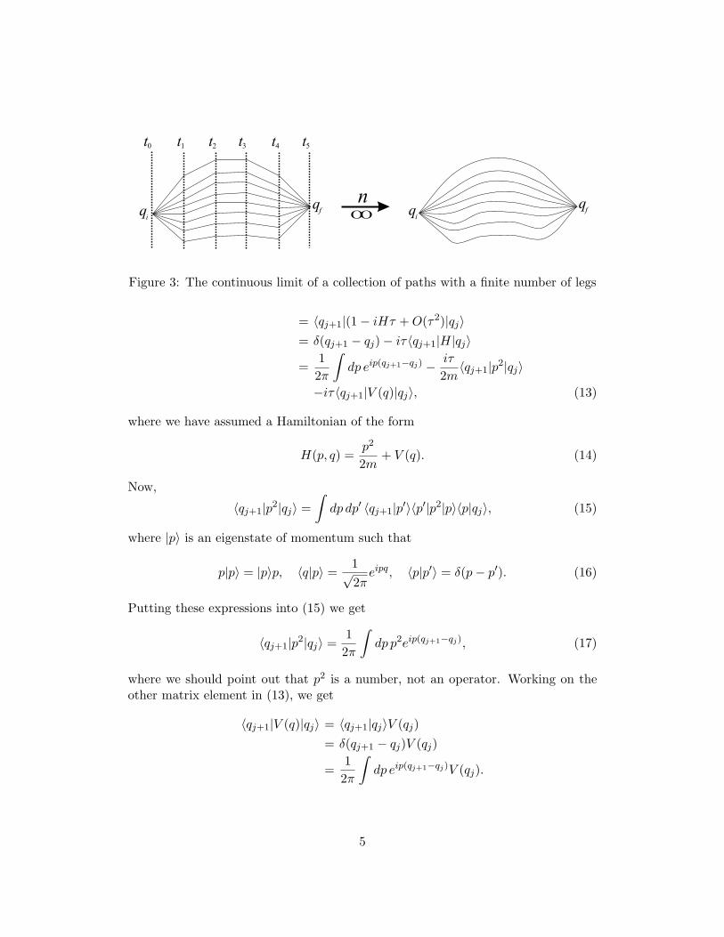
We take the limit n →∞ to obtain an expression for the propagator as a sum overinfinite-legged paths, as seen in figure 3. We can calculate the propagator for smalltime intervals τ = tj+1 − tj for some j between 1 and n− 1. We have

〈qj+1, tj+1|qj , tj〉 = 〈qj+1|e−iHtj+1e+iHtj |qj〉

4

t0 t1 t2 t3 t4 t5

qi

qf q

i

qf

nOO

Figure 3: The continuous limit of a collection of paths with a finite number of legs

= 〈qj+1|(1− iHτ + O(τ2)|qj〉= δ(qj+1 − qj)− iτ〈qj+1|H|qj〉=

12π

∫dp eip(qj+1−qj) − iτ

2m〈qj+1|p2|qj〉

−iτ〈qj+1|V (q)|qj〉, (13)

where we have assumed a Hamiltonian of the form

H(p, q) =p2

2m+ V (q). (14)

Now,

〈qj+1|p2|qj〉 =∫

dp dp′ 〈qj+1|p′〉〈p′|p2|p〉〈p|qj〉, (15)

where |p〉 is an eigenstate of momentum such that

p|p〉 = |p〉p, 〈q|p〉 =1√2π

eipq, 〈p|p′〉 = δ(p− p′). (16)

Putting these expressions into (15) we get

〈qj+1|p2|qj〉 =12π

∫dp p2eip(qj+1−qj), (17)

where we should point out that p2 is a number, not an operator. Working on theother matrix element in (13), we get

〈qj+1|V (q)|qj〉 = 〈qj+1|qj〉V (qj)= δ(qj+1 − qj)V (qj)

=12π

∫dp eip(qj+1−qj)V (qj).

5

Putting it all together

〈qj+1, tj+1|qj , tj〉 =12π

∫dp eip(qj+1−qj)

[1− iτH(p, qj) + O(τ2)

]

=12π

∫dp exp

[iτ

(p

∆qj

τ−H(p, qj)

)],

where ∆qj ≡ qj+1 − qj . Substituting this expression into (12) we get

〈qn, tn|q0, t0〉 =∫

dp0

n−1∏

i=1

dqi dpi

2πexp

i

n−1∑

j=0

τ

(pj

∆qj

τ−H(pj , qj)

) . (18)

In the limit n →∞, τ → 0, we have

n−1∑

j=0

τ →∫ tn

t0

dt,∆qj

τ→ dq

dt= q, dp0

n∏

i=1

dqi dpi

2π→ [dq] [dp], (19)

and

〈qn, tn|q0, t0〉 =∫

[dq] [dp] exp{

i

∫ tn

t0

dt [p q −H(p, q)]}

. (20)

The notation [dq] [dp] is used to remind us that we are integrating over all possiblepaths q(t) and p(t) that connect the points (q0, t0) and (qn, tn). Hence, we havesucceed in writing the propagator 〈qn, tn|q0, t0〉 as a functional integral over theall the phase space trajectories that the particle can take to get from the initialto the final points. It is at this point that we fully expect the reader to scratchtheir heads and ask: what exactly is a functional integral? The simple answer is aquantity that arises as a result of the limiting process we have already described.The more complicated answer is that functional integrals are beasts of a rathervague mathematical nature, and the arguments as to their standing as well-behavedentities are rather nebulous. The philosophy adopted here is in the spirit of manymathematically controversial manipulations found in theoretical physics: we assumethat everything works out alright.

The argument of the exponential in (20) ought to look familiar. We can bringthis out by noting that

12π

∫dpi e

iτhpi

∆qiτ−H(pi,qi)

i=

12π

exp

{iτ

[m

2

(∆qi

τ

)2

− V (qi)

]}

×∫

dpi exp

[− iτ

2m

(p− m∆qi

τ

)2]

=( m

2πiτ

)1/2exp

{iτ

[m

2

(∆qi

τ

)2

− V (qi)

]}.

6

Using this result in (18) we obtain

〈qn, tn|q0, t0〉 =( m

2πiτ

)n/2∫ n−1∏

i=1

dqi exp

i

n−1∑

j=0

τ

[m

2

(∆qj

τ

)2

− V (qj)

]

→ N

∫[dq] exp

[i

∫ tn

t0

dt

(12mq2 − V (q)

)], (21)

where the limit is taken, as usual, for n → ∞ and τ → 0. Here, N is an infiniteconstant given by

N = limn→∞

( m

2πiτ

)n/2. (22)

We won’t worry too much about the fact that N diverges because we will laternormalize our transition amplitudes to be finite. Recognizing the Lagrangian L =T − V in equation (21), we have

〈qn, tn|q0, t0〉 = N

∫[dq] exp

[i

∫ tn

t0

L(q, q) dt

]= N

∫[dq] eiS[q], (23)

where S is the classical action, given as a functional of the trajectory q = q(t).Hence, we see that the propagator is the sum over paths of the amplitude eiS[q],which is the amplitude that the particle follows a given trajectory q(t). Historically,Feynman demonstrated that the Schrodinger equation could be derived from equa-tion (23) and tended to regard the relation as the fundamental quantity in quantummechanics. However, we have assumed in our derivation that the potential is afunction of q and not p. If we do indeed have velocity-dependent potentials, (23)fails to recover the Schrodinger equation. We will not go into the details of how tofix the expression here, we will rather heuristically adopt the generalization of (23)for our later work in with quantum fields3.

An interesting consequence of (23) is seen when we restore ~. Then

〈qn, tn|q0, t0〉 = N

∫[dq] eiS[q]/~. (24)

The classical limit is obtained by taking ~→ 0. Now, consider some trajectory q0(t)and neighbouring trajectory q0(t)+δq(t), as shown in figure 4. The action evaluatedalong q0 is S0 while the action along q0+δq is S0+δS. The two paths will then makecontributions exp(iS0/~) and exp[i(S0 + δS)/~] to the propagator. For ~ → 0, thephases of the exponentials will become completely disjoint and the contributionswill in general destructively interfere. That is, unless δS = 0 in which case allneighbouring paths will constructively interfere. Therefore, in the classical limitthe propagator will be non-zero for points that may be connected by a trajectory

3The generalization of velocity-dependent potentials to field theory involves the quantization ofnon-Abelian gauge fields

7

q t( )

q t q t( ) + ( )d

q

q

i

f

Figure 4: Neighbouring particle trajectories. If the action evaluated along q(t) isstationary (i.e. δS = 0), then the contribution of q(t) and it’s neighbouring pathsq(t) + δq(t) to the propagator will constructively interfere and reconstruct the clas-sical trajectory in the limit ~→ 0

.

satisfying δS[q]|q=q0 ; i.e. for paths connected by classical trajectories determined byNewton’s 2nd law. We have hence seen how the classical principle of least actioncan be understood in terms of the path integral formulation of quantum mechanicsand a corresponding principle of stationary phase.

3 Perturbation theory, the scattering matrixand Feynman rules

In practical calculations, it is often impossible to solve the Schrodinger equationexactly. In a similar manner, it is often impossible to write down analytic expressionsfor the propagator 〈qf , tf |qi, ti〉 for general potentials V (q). However, if one assumesthat the potential is small and that the particle is nearly free, one makes goodheadway by using perturbation theory. We follow section 5.2 in Ryder [1].

In this section, we will go over from the general configuration coordinate q tothe more familiar x, which is just the position of the particle in a one-dimensionalspace. The extension to higher dimensions, while not exactly trivial, is not difficultto do. We assume that the potential that appears in (23) is “small”, so we mayperform an expansion

exp[−i

∫ tn

t0

V (x, t) dt

]= 1− i

∫ tn

t0

V (x, t) dt− 12!

[∫ tn

t0

V (x, t) dt

]2

+ · · · . (25)

We adopt the notation that K = K(xn, tn; x0, t0) = 〈xn, tn|x0, t0〉. Inserting theexpansion (25) into the propagator, we see that K possesses and expansion of theform:

K = K0 + K1 + K2 + · · · (26)

8

The K0 term is

K0 = N

∫[dx] exp

[i

∫12mx2 dt

]. (27)

If we turned off the potential, the full propagator would reduce to K0. It is for thisreason that we call K0 the free particle propagator, it represents the amplitude thata free particle known to be at x0 at time t0 will later be found at xn at time tn.Going back to the discrete expression:

K0 = limn→∞

( m

2πiτ

)n/2∫ n−1∏

i=1

dxi exp

imτ

2

n−1∑

j=0

(xj+1 − xj)2

. (28)

This is a doable integral because the argument of the exponential is a simplequadratic form. We can hence diagonalize it by choosing an appropriate rotation ofthe xj Cartesian variables of integration. Conversely, we can start calculating forn = 2 and solve the general n case using induction. The result is

K0 = limn→∞

( m

2πiτ

)n/2 1n1/2

(2πiτ

m

)(n−1)/2

exp[im(xn − x0)2

2nτ

]. (29)

Now, (tn − t0)/n = τ , so we finally have

K0(xn − x0, tn − t0) =[

m

2πi(tn − t0)

]1/2

exp[im(xn − x0)2

2(tn − t0)

], tn > t0. (30)

Here, we’ve noted that the substitution nτ = (tn − t0) is only valid for tn > t0. Infact, if K0 is non-zero for tn > t0 it must be zero for t0 > tn. To see this, we notethat the calculation of K0 involved integrations of the form:

∫ ∞

−∞eiαx2

dx =12

∫ ∞

0eiαx2

dx

=i−1/2

4

∫ i∞

0

eαs

s1/2ds

=i−1/2

4

∫ i∞

−i∞Θ(−is)

eαs

s1/2ds,

where α ∝ sign(τ) = sign(tn − t0). Now, we can either choose the branch of s−1/2

to be in either the left- or righthand part of the complex s-plane. But, we needto complete the contour in the lefthand plane if α > 0 and the righthand plane ifα < 0. Hence, the integral can only be non-zero for one case of the sign of α. Thechoice we have implicitly made is the the integral is non-zero for α ∝ (tn − t0) > 0,hence it must vanish for tn < t0. When we look at equation (8) we see that K0

is little more than a type of kernel for the integral solution of the free-particleSchrodinger equation, which is really a statement about Huygen’s principle. Our

9

choice of K0 obeys causality in that the configuration of the field at prior timesdetermines the form of the field in the present. We have hence found a retardedpropagator. The other choice for the boundary conditions obeyed by K0 yieldsthe advanced propagator and a version of Huygen’s principle where future fieldconfigurations determine the present state. The moral of the story is that, if wechoose a propagator that obeys casuality, we are justified in writing

K0(x, t) = Θ(t)[ m

2πit

]1/2exp

[imx2

2t

]. (31)

Now, we turn to the calculation of K1:

K1 = −iN

∫[dx] exp

[i

∫12mx2 dt

] ∫dt V (x(t), t). (32)

Moving again to the discrete case:

K1 = −iβn/2

∫dx1 · · · dxn−1 exp

imτ

2

n−1∑

j=0

(xj+1 − xj)2

n−1∑

i=1

τV (xi, ti), (33)

where β = m/2πiτ and the limit n → ∞ is understood. Let’s take the sum over i(which has replaced the integral over t) in front of the spatial integrals. Also, let’ssplit up the sum over j in the exponential to a sum running from 0 to i − 1 and asum running from i to n− 1. Then

K1 = −in−1∑

i=1

τ

∫dxi β

i/2

∫dx1 · · · dxi−1 exp

imτ

2

i−1∑

j=0

(xj+1 − xj)2

V (xi, ti)

×β(n−i)/2

∫dxi+1 · · · dxn−1 exp

imτ

2

n−1∑

j=i

(xj+1 − xj)2

. (34)

We recognize two factors of the free-particle propagator in this expression, whichallows us to write

K1 = −in−1∑

i=1

τ

∫dxK0(x− x0, ti − t0)V (x, ti)K0(xn − x, tn − ti). (35)

Now, we can replace∑n−1

i=1 τ by∫ tnt0

dt and ti → t in the limit n → ∞. SinceK0(x−x0, t− t0) = 0 for t < t0 and K0(xn−x, tn− t) for t > tn, we can extend thelimits on the time integration to ±∞. Hence,

K1 = −i

∫dx dtK0(xn − x, tn − t)V (x, t)K0(x− x0, t− t0). (36)

10

In a similar fashion, we can derive the expression for K2:

K2 =(−i)2

2!βn/2

∫dx1 · · · dxn−1 exp

imτ

2

n−1∑

j=0

(xj+1 − xj)2

(37)

×n−1∑

i=1

τV (xi, ti)n−1∑

k=1

τV (xk, tk). (38)

We would like to play the same trick that we did before by splitting the sum overj into three parts with the potential terms sandwiched in between. We need toconstruct the middle j sum to go from an early time to a late time in order to replaceit with a free-particle propagator. But the problem is, we don’t know whether ticomes before or after tk. To remedy this, we split the sum over k into a sum from1 to i − 1 and then a sum from i to n − 1. In each of those sums, we can easilydetermine which comes first: ti or tk. Going back to the continuum limit:

K2 =(−i)2

2!

∫dx1 dx2

∫ tn

t0

dt1

[∫ t1

t0

dt2K0(xn − x1, tn − t1)

×V (x1, t1)K0(x1 − x2, t1 − t2)V (x2, t2)K0(x2 − x0, t2 − t0)

+∫ tn

t1

dt2K0(xn − x2, tn − t2)V (x2, t2)K0(x2 − x1, t2 − t1)

×V (x1, t1)K0(x1 − x0, t1 − t0)]

(39)

But, we can extend the limits on the t2 integration to t0 → tn by noting the middlepropagator is zero for t2 > t1. Similarly, the t2 limits on the second integral canbe extended by observing the middle propagator vanishes for t1 > t2. Hence, bothintegrals are the same, which cancels the 1/2! factor. Using similar arguments, thelimits of both of the remaining time integrals can be extended to ±∞ yielding ourfinal result:

K2 = (−i)2∫

dx1 dx2 dt1 dt2 K0(xn − x2, tn − t2)V (x2, t2)

×K0(x2 − x1, t2 − t1)V (x1, t1)K0(x1 − x0, t1 − t0). (40)

Higher order contributions to the propagator follow in a similar fashion. The generaljth order correction to the free propagator is

Kj = (−i)j

∫dx1 . . . dxj dt1 . . . dtj K0(xn − xj , tn − tj)

×V (xj) · · ·V (x1)K0(x1 − x0, t1 − t0). (41)

We would like to apply this formalism to scattering problems where we assumethat the particle is initially in a plane wave state incident on some localized potential.

11

As t → ±∞, we assume the potential goes to zero, which models the fact that theparticle is far away from the scattering region in the distant past and the distantfuture. We go over from one to three dimensions and write

ψ(xf , tf ) =∫

dxiK0(xf − xi, tf − ti)ψ(xi, ti)

−i

∫dxi dx dtK0(xf − x, tf − t)

×V (x, t)K0(x− xi, t− ti)ψ(xi, ti) + · · · (42)

We push ti into the distant past, where the effects of the potential may be ignored,and take the particle to be in a plane wave state:

ψin(xi, ti) =1√V

e−ipi·xi , (43)

where we have used a box normalization with V being the volume of the box andpi ·x = Eiti−pi ·xi. The “in” label on the wavefunction is meant to emphasize thatit is the form of ψ before the particle moves into the scattering region. We want tocalculate the first integral in (42) using the 3D generalization of (31):

K0(x, t) = −iΘ(t)(

λ

π

)3/2

eλx2, (44)

where λ = im/2t. Hence,

∫dxiK0(xf − xi, tf − ti)ψin(xi, ti) = − i√

V

(λ

π

)3/2

×e−iEiti

∫dxie

λ(xf−xi)2+ipi·xi . (45)

This integral reduces to ψin(xf , tf ) as should have been expected, because K0 is thefree particle propagator and must therefore propagate plane waves into the futurewithout altering their form. We also push tf into the infinite future where the effectsof the potential can be ignored. Then,

ψ+(xf , tf ) = ψin(xf , tf )− i

∫dxi dx dtK0(xf − x, tf − t)

×V (x, t)K0(x− xi, t− ti)ψin(xi, ti) + · · · (46)

The “+” notation on ψ is there to remind us that ψ+ is the form of the wave functionafter it interacts with the potential. What we really want to do is Fourier analyzeψ+(xf , tf ) into momentum eigenstates to determine the probability amplitude fora particle of momentum pi becoming a particle of momentum pf after interacting

12

with the potential. Defining ψout(xf , tf ) as a state of momentum pf in the distantfuture:

ψout(xf , tf ) =1√V

e−ipf ·xf , (47)

we can write the amplitude for a transition from pi to pf as

Sfi = 〈ψout|ψ+〉. (48)

Inserting the unit operator 1 =∫

dxf |xf , tf 〉〈xf , tf | into (48) and using the propa-gator expansion (46), we obtain

Sfi = δ(pf − pi)− i

∫dxi dxf dx dt ψ∗out(xf , tf )K0(xf − x, tf − t)

×V (x, t)K0(x− xi, t− ti)ψin(xi, ti) + · · · (49)

The amplitude Sfi is the fi component of what is known as the S or scatteringmatrix. This object plays a central role in scattering theory because it answers allthe questions that one can experimentally ask about a physical scattering process.What we have done is expand these matrix elements in terms of powers of thescattering potential. Our expansion can be given in terms of Feynman diagramsaccording to the rules:

1. The vertex of this theory is attached to two legs and a spacetime point (x, t).

2. Each vertex comes with a factor of −iV (x, t).

3. The arrows on the lines between vertices point from the past to the future.

4. Each line going from (x, t) to (x′, t′) comes with a propagator K0(x′−x, t′−t).

5. The past external point comes with the wavefunction ψin(xi, ti), the futureone comes with ψ∗out(xf , tf ).

6. All spatial coordinates and internal times are integrated over.

Using these rules, the S matrix element may be represented pictorially as in figure 5.We note that these rules are for configuration space only, but we could take Fouriertransforms of all the relevant quantities to get momentum space rules. Obviously,the Feynman rules for the Schrodinger equation do not result in a significant sim-plification over the raw expression (49), but it is important to notice how they werederived: using simple and elegant path integral methods.

13

x , ti i

x , tf f

x , ti i

x , tf f

x , t1 1

x , t2 2

x , ti i

x , tf f

x , t1 1

Sfi = ++ + …

Figure 5: The expansion of Sfi in terms of Feynman diagrams

4 Sources, vacuum-to-vacuum transitions andtime-ordered products

We now consider a alteration of the system Lagrangian that models the presenceof a time-dependent “source”. Our discussion follows section 5.5 of Ryder [1] andchapters 1 and 2 of Brown [3]. In this context, we call any external agent thatmay cause a non-relativistic system to make a transition from one energy eigenstateto another a “source”. For example, a time-dependent electric field may induce acharged particle in a one dimensional harmonic oscillator potential to go from oneeigenenergy to another. In the context of field theory, a time-dependent source mayresult in spontaneous particle creation4. In either case, the source can be modeledby altering the Lagrangian such that

L(q, q) → L(q, q) + J(t)q(t). (50)

The source J(t) will be assumed to be non-zero in a finite interval t ∈ [t1, t2]. Wetake T2 > t2 and T1 < t1. Given that the particle was in it’s ground state atT1 → −∞, what is the amplitude that the particle will still be in the ground stateat time T2 →∞?

To answer that question, consider

〈Q2, T2|Q1, T1〉J =∫

dq1 dq2〈Q2, T2|q2, t2〉〈q2, t2|q1, t1〉J〈q1, t1|Q1, T1〉

=∫

dq1 dq2〈Q2|e−iHT2eiHt2 |q2〉〈q2, t2|q1, t1〉J×〈q1|e−iHt1eiHT1 |Q1〉

=∑mn

∫dq1 dq2〈Q2|e−iHT2 |m〉〈m|eiHt2 |q2〉〈q2, t2|q1, t1〉J

×〈q1|e−iHT1 |n〉〈n|eiHt1 |Q1〉4cf. PHYS 703 March 14, 2000 lecture

14

T

Te-id

-d

-dJ = 0

J = 0

J = 0 t2

t1

Figure 6: The rotation of the time axis needed to isolate the ground state contribu-tion to the propagator

=∑mn

e−i(EnT2−EmT1)φm(Q2)φ∗n(Q1)

×∫

dq1 dq2 φ∗m(q2, t2)〈q2, t2|q1, t1〉Jφn(q1, t1),

where we have introduced a basis of energy eigenstates H|n〉 = En|n〉 and energyeigenfunctions φn(q, t) = e−iEnt〈q|m〉 with φn(q) = 〈q|n〉. The J subscripts on thepropagators remind us that the source is to be accounted for. It is important tonote that φn(q) is only a true eigenfunction for times when the source is not acting;i.e. prior to t1 and later than t2. The integral on the last line can be thought ofas a wavefunction, φn(q1, t1), that is propagated through the time when the sourceis acting by 〈q2, t2|q1, t1〉J , and is then dotted with a wavefunction φ∗m(q2, t2). But,φn(q1, t1) and φ∗m(q2, t2) are energy eigenfunctions for times before and after thesource, respectively. Hence, the integral is the amplitude that an energy eigenstate|n〉 will become an energy eigenstate |m〉 through the action of the source. Now,let’s perform a rotation of the time-axis in the complex plane by some small angle−δ (δ > 0), as shown in figure 6. Under such a transformation

T1 → T1 + i|T1|δ (51)T2 → T2 − i|T2|δ, (52)

where we have chosen the axis of rotation to lie between T1 and T2. We seethat the exponential term e−i(EnT2−EmT1) will acquire a damping that goes likee−δ(En|T2|+Em|T1|). As we push T1 → −∞ and T2 → ∞, the damping will becomeinfinite for each term in the sum, except for the ground state which we can set tohave an energy of E0 ≥ 0. Therefore,

limT→∞ e−iδ

〈Q2, T |Q1,−T 〉J = e−iE0(T2−T1)φ0(Q2)φ∗0(Q1) (53)

×∫

dq1 dq2 φ∗0(q2, t2)〈q2, t2|q1, t1〉Jφ0(q1, t1), δ > 0,

where we have set T2 = −T1 = T for convenience. Now, if we take t2 and t1 to ±∞respectively, the integral reduces to the amplitude that a wavefunction which has

15

the form of φ0(q) in the distant past will still have the form of φ0(q) in the distantfuture. In other words, it is the ground-to-ground state transition amplitude, whichwe denote by

〈0,∞|0,−∞〉J ∝ limT→∞ e−iδ

〈Q2, T |Q1,−T 〉J , (54)

where the constant of proportionality depends on Q1, Q2 and T . Now, insteadof rotating the contour of the the time-integration, we could have added a smallterm −iεq2/2 to the Hamiltonian. Using first order perturbation theory, this shiftsthe energy levels by an amount δEn = −iε〈n|q2|n〉/2. For most problems (i.e. theharmonic oscillator, hydrogen atom), the expectation value of q2 increases withincreasing energy. Assuming that this is the case for the problem we are doing, wesee that the first order shift in the eigenenergy accomplishes the same thing as therotation of the time axis in (54). But, subtracting iεq2/2 from H is the same thingas adding iεq2/2 from L5. Therefore,

〈0,∞|0,−∞〉J ∝∫

[dQ] exp{

i

∫ ∞

−∞dt

[L(Q, Q) + JQ +

12iεq2

]}. (55)

Finally, want to normalize this result such that if the source is turned off, theamplitude 〈0,∞|0,−∞〉 is unity. Defining

Z[J ] =

∫[dQ] exp

{i∫∞−∞ dt

[L(Q, Q) + JQ + 1

2 iεQ2]}

∫[dQ] exp

{i∫∞−∞ dt

[L(Q, Q) + 1

2 iεQ2]} , (56)

we have〈0,∞|0,−∞〉J = Z[J ]. (57)

Before moving on the the next section, we would like to establish a result that willprove very useful later when we consider field theories. We first define the functionalderivative of Z[J ] with respect to J(t′). Essentially, the functional derivative of afunctional f [y], where y = y(x), is the derivative of the discrete expression withrespect to the value of y at a given x. For example, the discrete version of Z[J ] is

Z (τJ(t0), τJ(t1) . . . τJ(tn−1)) ∝∫

exp

iτ

n−1∑

j=0

[L(Qj , Qj)

+ J(tj)Qj +12iεQ2

j

]}n−1∏

i=1

dQi, (58)

where we have indicated that the discrete version of Z[J ] is an ordinary function of nvariables τJ(tj) and omitted the normalization factor. We have explicitly included

5An alternative procedure for singling out the ground state contribution comes from consideringt to be purely imaginary, i.e. consideration of Euclidean space. This is discussed in the next section.

16

the weighting factor τ with each of the discrete variables to account for the factthat as n → ∞, each J(tk) covers a smaller and smaller portion of the integrationinterval. The functional derivative of Z[J ] with respect to J(tk) is then the partialderivative of the discrete expression with respect to τJ(tk). Going back to thecontinuum limit, we write the functional derivative of Z[J ] with respect to Q(t1) as:

δZ[J ]δJ(t1)

∝ i

∫[dQ]Q(t1) exp

{i

∫ ∞

−∞dt

[L(Q, Q) + JQ +

12iεQ2

]}. (59)

In a similar fashion, we have

δnZ[J ]δJ(t1) · · · δJ(tn)

∝ in∫

[dQ]Q(t1) · · ·Q(tn)

× exp{

i

∫ ∞

−∞dt

[L(Q, Q) + JQ +

12iεQ2

]}. (60)

We notice a similarity between this expression and the expression from statisticalmechanics that gives the average value of a microscopic variable in the canonicalensemble. We argue that equation (60) gives the exact same thing: the expectationvalue of Q(t1) · · ·Q(tn). There is one wrinkle, however, which we now proceed tooutline. Consider, with tk > tk′ ,

〈qf , tf |q(tk)q(tk′)|qi, ti〉 =∫

dq1 · · · dqn−1〈qf , tf |qn−1, tn−1〉 · · ·〈qk, tk|q(tk)|qk−1, tk−1〉 · · · 〈qk′ , tk′ |q(tk′)|qk′−1, tk′−1〉· · · 〈q1, t1|qi, ti〉

=∫

dq1 · · · dqn−1 q(tk)q(tk′)〈qf , tf |qn−1, tn−1〉 · · ·〈q1, t1|qi, ti〉. (61)

By pushing ti → −∞ e−iδ and tf → ∞ e−iδ, we can repeat our previous manipula-tions to show that

∫dq1 · · · dqn−1 q(tk)q(tk′)〈qf ,∞ e−iδ|qn−1, tn−1〉 · · · 〈q1, t1|qi,−∞ e−iδ〉

= N

∫[dq]q(tk)q(tk′) exp

[i

∫ ∞ e−iδ

−∞ e−iδ

dtL(Q, Q)

], (62)

which follows directly from the arguments of section 2, and

〈qf ,∞ e−iδ|q(tk)q(tk′)|qi,−∞ e−iδ〉 ∝ 〈0|q(tk)q(tk′)|0〉, (63)

which follows from an argument similar to the one we used to calculate the matrixelement 〈0,∞|0,−∞〉J with t1 = tk′ , t2 = tk and J = 0. Just as before, the

17

rotation of the time axis can be achieved by adding iεq2/2 to the Lagrangian. Thiscalculation cannot be repeated for the case tk > tk′ because the order of q(tk)q(tk′)in 〈qf , tf |q(tk)q(tk′)|qi, ti〉 cannot be switched without introducing terms involvingthe commutator of H and q. But, in order to perform the decomposition (61), weneed the late q operator appearing to the left of the earlier q operator. What thismeans is that we must be considering the time-ordered product of q(tk) and q(tk′).Putting all of this together along with the expression for the functional derivativesof Z[J ], we get

δ2Z[J ]δJ(tk)δJ(tk′)

∣∣∣∣J=0

= i2〈0|T [q(tk)q(tk′)]|0〉. (64)

This is easily generalized to the time order product of many q operators:

δnZ[J ]δJ(t1) · · · δJ(tn)

∣∣∣∣J=0

= in〈0|T [q(t1) · · · q(tn)]|0〉. (65)

We have demanded strict equality in these expression to ensure that the n = 0 casereturns 〈0|0〉 = 1. This is a very important formula for what follows.

5 Free scalar fields

We now move on to the quantum field theory of a scalar field φ(x). In this sectionwe draw on sections 6.1 and 6.3 of Ryder [1], chapter 2 of Popov [4] and section 3.2of Brown [3]. The classical field φ is assumed to satisfy the Klein-Gordon equation

(¤ + m2)φ = 0. (66)

We define the vacuum to vacuum transition probability for this theory by

〈0,∞|0,−∞〉J = Z[J ], (67)

where

Z[J ] =1Z0

∫[dφ] exp

{i

∫d4x

[L(φ) + J(x)φ +

12iεφ2

]}, (68)

with

Z0 =∫

[dφ] exp{

i

∫d4x

[L(φ) +

12iεφ2

]}. (69)

In this expressions, the measure [dφ] is meant to convey an integration over all fieldconfigurations, which can be achieved in practice by dividing spacetime into N4

points (tm, xi, yj , zk), with m, i, j, k = 1 . . . N . We can schematically merge all ofthese indices into a single one n = 1 . . . N4. The field is considered to be a collectionof N4 independent variables, and the functional integration [dφ] becomes

∫ ∏i dφi.

The functional Z[J ] represents the fundamental object in the theory. Knowledge ofthe form of Z[J ] allows us to derive all the results that we could hope to obtain from

18

experiments involving the field φ. Such grandiose statements need to be justified,which we now proceed to do.

We first substitute the Lagrangian appropriate to the Klein-Gordon equationinto the expression for Z[J ]:

Z[J ] =1Z0

∫[dφ] exp

(i

∫d4x

{12

[∂αφ∂αφ− (m2 − iε)φ2

]+ φJ

}). (70)

Integrating the ∂αφ∂αφ term by parts and using Gauss’ theorem to discard theboundary term (assuming φ → 0 at infinity) gives

Z[J ] =1Z0

∫[dφ] exp

(−i

∫d4x

{12φ(¤ + m2 − iε)φ− φJ

}). (71)

Regarding φ as an integration variable, we can change variables according to

φ(x) → φ(x) + φ0(x). (72)

Noting that ∫d4x φ¤φ0 =

∫d4xφ0¤φ (73)

using Gauss’ theorem and demanding that φ0 → 0 at infinity, we obtain

Z[J ] =1Z0

∫[dφ] exp

(−i

∫d4x

{12φ(¤ + m2 − iε)φ

+φ(¤ + m2 − iε)φ0 +12φ0(¤ + m2 − iε)φ0 − (φ + φ0)J

}). (74)

Let us demand that(¤ + m2 − iε)φ0 = J(x). (75)

We can solve this equation by introducing the Feynman propagator, which satisfies

(¤ + m2 − iε)∆F (x) = −δ4(x). (76)

Hence,

φ0 = −∫

∆F (x− y)J(y) d4y. (77)

We then obtain for Z[J ]:

Z[J ] =1Z0

exp[− i

2

∫J(x)∆F (x− y)J(y) d4x d4y

]

×∫

[dφ] exp[− i

2

∫φ(¤ + m2 − iε)φd4x

]. (78)

19

But we know Z[0] = 1, so we must have

Z0 =∫

[dφ] exp[− i

2

∫φ(¤ + m2 − iε)φd4x

]. (79)

This leads to our final expression:

Z[J ] = exp[− i

2

∫J(x)∆F (x− y)J(y) d4x d4y

]. (80)

Before we move forward, we would like to make a comment on the inclusion of theiεφ2/2 term in our expression for Z[J ]. The reader will recall that the reason that weadded this term was to simulate the effects of rotating the time axis by a small angle−δ in the complex plane. Instead of adding the ε-term, we can instead rotate thet axis by −π/2 so that t = −iτ . The metric becomes ηαβ = diag(−1,−1,−1,−1),which means that we are considering a Euclidean, not Lorentzian, manifold. In thatcase, the vacuum-to-vacuum transition amplitude is

Z[J ] =1Z0

∫[dφ] exp

(−

∫dτdx

{12

[(∂τφ)2 +∇φ2 + m2φ2

]− φJ

}), (81)

where ∇ is the del-operator of 3D vector calculus. For J = 0, the argument ofthe exponential is negative definite and the integral converges absolutely. So, insome sense, the rotation of the time axis ensures that the integrals in Z[J ] are wellbehaved. Another aspect the Euclidean manifold comes from the Euclidean versionof Feynman propagator, which satisfies:

(∂2τ +∇2 −m2)∆F (x) = δ4(x). (82)

Solving this in Euclidean Fourier space, we get

∆F (x) = − i

(2π)4

∫d4κ

e−iκ·x

κ2 + m2, (83)

where κ · x = κ0τ + k · x and κ2 = (κ0)2 + k2 (the i is there for convenience). If wechange variables according to κ0 = −ik0 and τ = it, we get

∆F (x) = − 1(2π)4

∫

C′d4k

e−ik·x

k2 −m2, (84)

where the k0 integration is to be performed along the contour C ′ shown in figure7. But, we can rotate the contour by 90o clockwise to C, which is the standardcontour used to calculate the Lorentzian Feynman propagator, defined by (76). Tosome extent, this explains why the Feynman propagator has the form that it does:it is a direct consequence of the need to rotate the time axis to isolate the vacuumcontributions to transition amplitudes and make path integrals converge.

20

=+w +w-w

-wRe( )k0 Re( )k0

Im( )k0 Im( )k0

C

C

Figure 7: Equivalent contours of integration for the calculation of Feynman propa-gator in the complex k0 plane. Note the poles at ±ω = ±

√|k|2 + m2.

We want to calculate the time-ordered products given by

1in

δnZ[J ]δJ(x1) · · · δJ(xn)

∣∣∣∣J=0

= 〈0|T [φ(x1) · · ·φ(xn)]|0〉. (85)

We recall from the canonical formulation of field theory that 〈0|T [φ(x)φ(y)]|0〉 isthe amplitude for the creation of a particle at y and its later destruction at x (orvice versa, depending on the times associated with x and y). Using (80) and ourpreviously mentioned notions of functional differentiation, we have

1i

δ

δJ(x1)Z[J ] = −Z[J ]

∫dy ∆F (x1 − y)J(y). (86)

The second order derivative is

1i

δ

δJ(x2)1i

δ

δJ(x1)Z[J ] = Z[J ]

∫dy1 ∆F (x1 − y1)J(y1)

∫dy2 ∆F (x2 − y2)J(y2)

+ i∆F (x1 − x2)Z[J ].

Continuing,

1i

δ

δJ(x3)1i

δ

δJ(x2)1i

δ

δJ(x1)Z[J ] =

− i∆F (x1 − x2)Z[J ]∫

dy3 ∆F (x3 − y3)J(y3)

− i∆F (x1 − x3)Z[J ]∫

dy2 ∆F (x2 − y2)J(y2)

− i∆F (x2 − x3)Z[J ]∫

dy1 ∆F (x1 − y1)J(y1)

21

− Z[J ]∫

dy1 dy2 dy3 ∆F (x1 − y1)J(y1)

× ∆F (x2 − y2)J(y2)∆F (x3 − y3)J(y3)

Finally, we write down the fourth order derivative:

1i

δ

δJ(x4)1i

δ

δJ(x3)1i

δ

δJ(x2)1i

δ

δJ(x1)Z[J ] = i∆F (x1 − x2)i∆F (x3 − x4)Z[J ]

+ i∆F (x1 − x3)i∆F (x2 − x4)Z[J ]

+ i∆F (x2 − x3)i∆F (x1 − x4)Z[J ]

+ other terms that vanish when J = 0.

When J = 0, these expression give us the following time-ordered products:

〈0|T [φ(x1)]|0〉 = 0 (87)〈0|T [φ(x1)φ(x2)]|0〉 = i∆F (x1 − x2) (88)

〈0|T [φ(x1)φ(x2)φ(x3)]|0〉 = 0 (89)〈0|T [φ(x1)φ(x2)φ(x3)φ(x4)]|0〉 = i∆F (x1 − x2)i∆F (x3 − x4)

+ i∆F (x1 − x3)i∆F (x2 − x4)+ i∆F (x1 − x4)i∆F (x2 − x3) (90)

We call 〈0|T [φ(x1) · · ·φ(xn)]|0〉 an n-point correlation function. Generalizing thepattern above to T products of more field operators, we find that if n is odd, then-point function vanishes. On the other hand, if n is even, the correlation func-tion reduces to the sum all possible permutations of products of 2-point functionsi∆F (x − y) with x, y ∈ {x1, . . . , xn}, x 6= y. When this result is derived fromcanonical methods, it is know as Wick’s Theorem.

It is interesting to interpret these results in terms of the Taylor series expansionof Z[J ] about J = 0. To make sense of this object, recall that the Taylor seriesexpansion of a function of a finite number of variables is

F (y1, . . . , yk) =∞∑

n=0

k∑

i1=1

· · ·k∑

in=1

1n!

yi1 . . . yik

∂nF

∂yi1 . . . ∂yin

∣∣∣∣yi=0

. (91)

This is expansion is taken about the zero of all of the independent variables. As-suming the variables are weighted appropriately, when we go to the continuum limitk →∞ we obtain that

F [y] =∞∑

n=0

1n!

∫dx1 · · · dxn y(x1) · · · y(xn)

δnF

δy(x1) . . . δy(xn)

∣∣∣∣y=0

. (92)

Using this expansion, we obtain

22

Z J[ ] = 1 + x1 x2

x1 x2

x3 x4

+ ++ +( (x1 x2

x3 x4

x1 x2

x3 x4

…

Figure 8: Pictorial representation of the free field generating functional Z[J ]

Z[J ] = 1 +i2

2!

∫dx1 dx2 J(x1)J(x2)i∆F (x1 − x2)

+i4

4!

∫dx1 dx2 dx3 dx4J(x1)J(x2)J(x3)J(x4)

×[i∆F (x1 − x2)i∆F (x3 − x4) + i∆F (x1 − x3)i∆F (x2 − x4)

+ i∆F (x1 − x4)i∆F (x2 − x3)]

+ · · · (93)

This result is depicted diagrammatically in figure 8. In this figure, we use thefollowing Feynman rules:

1. Each line is connected to a sink and a source.

2. Each sink or a source is labeled with a spacetime point.

3. A line running between x and y comes with a propagator i∆F (x− y).

4. Each source or sink attached to x comes with a factor iJ(x).

5. The collection of all graphs with n sources and sinks is multiplied by 1/n!.

6. All spacetimes coordinates are integrated over.

This first rule ensures that we only include diagrams with an even number of verticesand that we only consider disconnected graphs. The Feynman diagrams illustratethe correspondence of Z[J ] to the vacuum-to-vacuum transition probability beauti-fully. Each term in the graph involves the creation of a particle at some point andits destruction at a later point. The three terms in the 4-vertex graph account forall possible permutations of particle being created/destroyed at a pair of x1, x2, x3

or x4. What we would like to do now is move on to the more interesting case ofinteracting fields.

6 The generating functional for self-interacting fields

While free field theory has a certain amount of elegance to it, it is not terriblyinteresting. In this section, we consider a self-interacting field whose Lagrangian is

23

given by

L(φ) =12∂αφ∂αφ− 1

2m2φ2 + Lint(φ) = L0(φ) + Lint(φ). (94)

The discussion follows section 6.4 of Ryder [1]. Here, Lint(φ) is the Lagrangiandescribing the self interaction. The generating functional is

Z[J ] =

∫[dφ] exp

(iS + i

∫d4xJφ

)∫

[dφ]eiS, (95)

where S is the classical action

S =∫

d4x [L0(φ) + Lint(φ)] = S0 + Sint. (96)

We have dropped the iεφ2/2 term used to single out the ground state, which we canrationalize by the rotation of the time axis. In this section, we will write the freefield propagator as

Z0[J ] =

∫[dφ] exp

(iS0 + i

∫d4xJφ

)∫

[dφ]eiS0. (97)

We would like to write Z[J ] in a form particularly useful for calculations. Wecan’t really reproduce the manipulations of the last section because the Lint in theaction S introduces difficulties when the shift φ → φ + φ0 is performed. We willinstead derive a differential equation satisfied by Z[J ] and then solve it in termsof J(x) and the Feynman propagator. The result will be something that we mighthave guessed intuitively. What is the equation satisfied by the free field propagator?Now, we know that

1i

δ

δJ(x)Z0[J ] = −Z0[J ]

∫dy ∆F (x− y)J(y). (98)

We operate on both sides with ¤x+m2 and use the defining relation for the Feynmanpropagator (76) to get:

(¤x + m2)1i

δ

δJ(x)Z0[J ] = J(x)Z0[J ]. (99)

The is the differential equation satisfied by Z0[J ]. In order to find the differentialequation satisfied by Z[J ], let us define the functional

Z[φ] =eiS

∫[dφ] eiS

. (100)

Then

Z[J ] =∫

[dφ] Z[φ] exp(

i

∫d4xJφ

), (101)

24

which is the functional equivalent of the Fourier transform. We can functionallydifferentiate Z[φ] with respect to φ using

S =∫

d4x

[12∂αφ∂αφ− 1

2m2φ2 + Lint(φ)

]

= −∫

d4x

[12φ(¤ + m2)φ− Lint

], (102)

where Gauss’ theorem has been used. The superiority of the latter form is that wecan integrate twice by parts to change φ

−→¤φ into φ←−¤φ. So, when we functionally

differentiate, we can make sure that the φ being acted on by the ¤ operator isdifferent from the φ being acted on by the δ/δφ. We get

iδZ[φ]δφ(x)

= (¤ + m2)φ(x)Z[φ]− L′int(φ)Z[φ], (103)

whereL′int(φ) =

∂Lint

∂φ(104)

and ¤ = ¤x. We multiply both sides of (103) by exp[i∫

J(y)φ(y) d4y] and integrateover φ, i.e. we take the Fourier transform. The RHS of (103) becomes

RHS =1Z0

(¤ + m2)∫

[dφ]φ(x) exp[iS + i

∫J(y)φ(y) d4y

]

− 1Z0

∫[dφ]L′int(φ) exp

[iS + i

∫J(y)φ(y) d4y

], (105)

where we have writtenZ0 =

∫[dφ]eiS . (106)

Now, it’s easy to see

1i

δZ[J ]δJ(x)

=1Z0

∫[dφ]φ(x) exp

[iS + i

∫J(y)φ(y) d4y

], (107)

which leads to(

1i

δ

δJ(x)

)n

Z[J ] =1Z0

∫[dφ] φn(x) exp

[iS + i

∫J(y)φ(y) d4y

]. (108)

Now, we assume that L′int(φ) possesses a Taylor series expansion in φ. We can thenreproduce the second term in (105) by adding together a series of contributions ofthe form of (108). Hence,

RHS = (¤ + m2)1i

δZ[J ]δJ(x)

− L′int

(1i

δ

δJ(x)

)Z[J ]. (109)

25

The Fourier transform of the LHS of (103) becomes

LHS = i

∫[dφ]

δZ(φ)δφ(x)

exp[i

∫J(y)φ(y) d4y

]

= iZ(φ) exp[i

∫J(y)φ(y) d4y

] ∣∣∣∣φ→∞

−i

∫[dφ]Z(φ)

δ

δφ(x)exp

[i

∫J(y)φ(y) d4y

]

=∫

[dφ]J(x)Z(φ) exp[i

∫J(y)φ(y) d4y

]

= J(x)Z[J ]. (110)

In the second line we have performed a functional integration by parts, which followsfrom the fact that the functional derivative satisfies the product rule and functionalintegral obeys the fundamental theorem of calculus. The boundary term must vanishas φ →∞ because if it didn’t, the integral for Z[J ] would diverge. Putting togetherour formulae for the LHS and RHS of the Fourier transform of (103):

(¤ + m2)1i

δZ[J ]δJ(x)

− L′int

(1i

δ

δJ(x)

)Z[J ] = J(x)Z[J ]. (111)

This is the differential equation satisfied by Z[J ]. We see that if the interactingLagrangian is set to zero, the result reduces to (99).

We will assume a solution of the differential equation of the form

Z[J ] = N exp[i

∫d4xLint

(1i

δ

δJ

)]Z0[J ] (112)

partly because this is what we might expect from L = L0+Lint if we replace −iδ/δJwith φ, as we usually do, partly because we know it’s the right answer. As usual,N is a normalizing factor. Let’s first establish and identity:

exp[−i

∫d4yLint

(1i

δδJ(y)

)]J(x) exp

[i∫

d4yLint

(1i

δδJ(y)

)]

= J(x)− L′int

(1i

δδJ(x)

). (113)

The first step is to notice that the commutator of Ji and ∂/∂Jk when acting on afunction of (J1, . . . , Jn) is given by the well known relation

[Ji,

1i

∂

∂Jk

]= iδik. (114)

The continuum limit (n →∞) of this is[J(x),

1i

δ

δJ(y)

]= iδ(x− y). (115)

26

Now, it’s not hard to see that if A and B are operators whose commutator is anumber a, then

[A,B] = a,

[A,B2] = 2aB,

[A,B3] = 3aB2,

...[A,Bn] = naBn−1.

Hence, [J(x),

(1i

δ

δJ(y)

)n]= iδ(x− y)n

(1i

δ

δJ(y)

)n−1

. (116)

Assume that Lint(φ) possesses a Taylor series expansion

Lint(φ) = c0 + c1φ +12!

c2φ2 + · · · =

∞∑

n=0

1n!

cnφn. (117)

Since [A, (B + C)] = [A,B] + [A, C], we can write[J(x),

∞∑

n=0

1n!

cn

(1i

δ

δJ(y)

)n]

= iδ(x− y)∞∑

n=1

1(n− 1)!

cn

(1i

δ

δJ(y)

)n−1

. (118)

But

L′int(φ) =∞∑

n=0

n

n!cnφn−1 =

∞∑

n=1

1(n− 1)!

cnφn−1. (119)

Using this an integrating (118) with respect to y gives[J(x), i

∫d4yLint

(1i

δ

δJ(y)

)]= −L′int

(1i

δ

δJ(x)

). (120)

where we have scaled Lint by i. Finally, note that the Hausdorff formula gives

e−BAeB = A + [A, B] (121)

when [A,B] is a number. Putting (120) into (121) with A = J(x) and B =i∫

d4yLint (−iδ/δJ(y)) yields (113).Using our assumed form for Z[J ] (112) and the identity (113) we get

J(x)Z[J ] = NJ(x) exp[i

∫d4yLint

(1i

δ

δJ(y)

)]Z0[J ]

= N exp[i

∫d4yLint

(1i

δ

δJ(y)

)][J(x)− L′int

(1i

δ

δJ(x)

)]Z0[J ]

27

= N exp[i

∫d4yLint

(1i

δ

δJ(y)

)](¤x + m2)

1i

δ

δJ(x)Z0[J ]

−L′int

(1i

δ

δJ(x)

)N exp

[i

∫d4yLint

(1i

δ

δJ(y)

)]Z0[J ]

= (¤x + m2)1i

δZ[J ]δJ(x)

− L′int

(1i

δ

δJ(x)

)Z[J ].

In going from the second to the third line, we have used the differential equationsatisfied by Z0[J ] (99). This result is just the differential equation (111), whichconfirms that we can write

Z[J ] =exp

[i∫

d4xLint

(1i

δδJ(x)

)]Z0[J ]

exp[i∫

d4xLint

(1i

δδJ(x)

)]Z0[J ]

∣∣∣J=0

(122)

where we have

Z0[J ] = exp[− i

2

∫J(x)∆F (x− y)J(y) d4x d4y

]. (123)

With these two equations, we have succeeding in writing down the generating func-tional entirely in terms of the source J and the Feynman propagator ∆F .

7 φ4 and φ3 theory

We would like to demonstrate the calculation of the generating functional Z[J ] andsome n-point functions in the case of self-interacting φ4 and φ3 theory. We followsection 6.5 of Ryder [1] and chapter 2 of Popov [4]. We first consider φ4 theory,which has the interacting Lagrangian:

Lint(φ) = − λ

4!φ4. (124)

It goes without saying that λ is small. The generating functional Z4[J ] for φ4 is

Z4[J ] =exp

[− iλ

4!

∫d4z

(1i

δδJ(z)

)4]

Z0[J ]

exp[− iλ

4!

∫d4z

(1i

δδJ(x)

)4]

Z0[J ]∣∣∣J=0

(125)

The numerator of Z4[J ] is, to first order in λ, is:

numZ4[J ] =

[1− iλ

4!

∫d4z

(1i

δ

δJ(z)

)4

+ · · ·]

Z0[J ]. (126)

28

Performing the functional differentiation, we obtain

numZ4[J ] =

{1− iλ

4!

∫d4z

[−3∆2

F (0) + 6i∆F (0)(∫

d4x∆F (z − x)J(x))2

+(∫

d4x∆F (z − x)J(x))4

]+ · · ·

}Z0[J ], (127)

where we have written ∆F (z − z) = ∆F (0)6. We also get

denomZ4[J ] = numZ4[J ]∣∣∣∣J=0

={

1− iλ

4!

∫d4z

[−3∆2F (0)

]+ · · ·

}Z0[J ]. (128)

Putting the two results together yields, to order λ, we have:

Z4[J ] =

{1− iλ

4!

∫d4z

[6i∆F (0)

(∫d4x∆F (z − x)J(x)

)2

+(∫

d4x∆F (z − x)J(x))4

]+ · · ·

}Z0[J ], (129)

Now, let’s do the same thing for φ3 theory, where the interacting Lagrangian is

Lint(φ) = − λ

3!φ3. (130)

The numerator of the generating functional is

numZ3[J ] = exp

[− iλ

3!

∫d4z

(1i

δ

δJ(z)

)3]

Z0[J ]. (131)

Expanding to order λ, we get

numZ3[J ] ={

1− iλ

3!

∫d4z

[−3i∆F (0)

∫d4x∆F (z − x)J(x)

−(∫

d4x∆F (z − x)J(x))3

]+ · · ·

}Z0[J ]. (132)

If we set J = 0, the above reduces to unity. So, the denominator of Z3[J ] is 1, tofirst order in λ, which yields:

Z3[J ] ={

1− iλ

3!

∫d4z

[−3i∆F (0)

∫d4x∆F (z − x)J(x)

−(∫

d4x∆F (z − x)J(x))3

]+ · · ·

}Z0[J ]. (133)

6The Feynman propagator evaluated at zero is, of course, infinite. It’s inclusion in the generatingfunctional represents the infinite self-energy of particles in the theory and must be regulated byrenormalization, which we will not consider here.

29

…il

6- +

l

2x1 z +Z J[ ] = 13

z

x1

x2

x3

l

4+

x1 x2z

z …+Z J[ ] = 14

x1 x2

x3 x4

il

24-

Figure 9: Pictorial representation of the generating functional for φ4 and φ3 theoryrespectively

We can represent the two generating functionals Z4[J ] and Z3[J ] diagrammati-cally with the following Feynman rules:

1. The spacetime point zi is associated with internal points, all other variablesgo with external points (recall that zi is the coordinate that occurred in theinteracting Lagrangian).

2. A line between x and z comes with a propagator ∆F (x− z).

3. Each internal point comes with a factor of iλ/4! for φ4 theory, iλ/3! for φ3

theory.

4. External points x come with a factor J(x).

5. Terms of the form ∆F (0) represent closed loops, or propagators who beginand end at the same point, joined to internal points.

6. All spacetime points are integrated over.

7. Each term in the series is multiplied by the free particle propagator Z0[J ].

These rules give the pictures in figure 9 for Z4[J ] and Z3[J ]. These diagrams stressthe general structure of the two theories. Because of the power of 4 in the interact-ing Lagrangian in φ4 theory, the vertices in the associated Feynman diagrams areattached to 4 legs. Similarly, the vertices in φ3 theory are attached to 3 legs. Apeculiarity of φ3 theory is the diagram with only one external point. As we will seebelow, this gives rise to a one point correlation function which means that particlesin φ3 can spontaneously self-destruct.

30

l

2-

x1 x2z

x1 x2…+i

il

4x1 z

…+

Figure 10: Pictorial representation of the two-point function 〈0|T [φ(x1)φ(x2)]|0〉4 forφ4 theory (top) and of the one-point function 〈0|T [φ(x1)]|0〉3 for φ3 theory (bottom)

Let’s calculate the 2-point function for φ4 theory:

〈0|T [φ(x1)φ(x2)]|0〉4 = − δ2Z4[J ]δJ(x2)δJ(x1)

∣∣∣∣J=0

. (134)

The functional differentiation is easy to do from (129) using the our previouslyderived formulae for derivatives of the free field propagator (87) – (90). The resultis

〈0|T [φ(x1)φ(x2)]|0〉4 = i∆F (x1 − x2)− λ

2∆F (0)

∫d4z ∆F (x1 − z)∆F (z − x2)

+ O(λ2). (135)

This can be turned into a Feynman diagram, as in figure 10, using rules similarto the ones for Z[J ], except now the only the internal points are integrated over.Figure 10 shows how the amplitude for the creation of a particle at point x1 and itslater destruction at x2 is modified by an (infinite) loop diagram to first-order in λin φ4 theory.

Now, let’s get the 2-point function in φ3 theory. It is simply calculated

〈0|T [φ(x1)φ(x2)]|0〉3 = − δ2Z3[J ]δJ(x2)δJ(x1)

∣∣∣∣J=0

= i∆F (x1 − x2) + O(λ2). (136)

This isn’t terribly interesting, we see that there are no corrections to the free fieldresult to this level in perturbation theory. We shouldn’t be surprised, there is noway to connect to external lines to a single vertex if the vertex must be attachedto three lines. However, there is a way to connect a vertex to one external line andone internal line, as shown in figure 10. This is borne out by the calculation of theone-point function:

〈0|T [φ(x1)]|0〉3 = −iδ2Z3[J ]δJ(x1)

∣∣∣∣J=0

=iλ

4∆F (0)

∫d4z ∆F (z − x1) + O(λ2). (137)

31

…l

4+ ++ +

x1z

x2 x3

x2z

x3 x1

x3z

x1 x2

-lz

x1

x2

x3 ( (Figure 11: Pictorial representation of 〈0|T [φ(x1)φ(x2)φ(x3)]|0〉3, the three pointfunction, for φ3 theory

Certainly a strange beast, this represents the amplitude of a particle being sponta-neously created out of the vacuum, all by itself7. We can also calculate the threepoint function

〈0|T [φ(x1)φ(x2)φ(x3)]|0〉3 = iδ2Z3[J ]

δJ(x3)δJ(x2)δJ(x1)

∣∣∣∣J=0

= −λ

∫d4z ∆F (z − x1)∆F (z − x2)∆F (z − x3)

+λ

4∆F (0)

∫d4z [∆F (z − x1)∆F (x2 − x3)

+ ∆F (z − x2)∆F (x3 − x1)+ ∆F (z − x3)∆F (x1 − x2)]. (138)

The first integral involves all the external legs attached to the same point, i.e. twoparticles merging into one or one particle splitting in two. The second integralis the product of free 2-point functions and the 1-point function we have alreadycalculated. The diagram is in figure 11.

We have hence shown how the generating functional and n-point functions canbe found from simple functional differentiation of equations (122) and (123) andexpressed in terms of Feynman diagrams. These diagrams can be converted intoscattering amplitudes via the LSZ reduction formula8:

〈p1, . . . ,pn,+∞|q1, . . . ,qm,−∞〉 = disconnected terms

+ (i)n+m

∫dy1 · · · dyn dx1 · · · dxm

× ei(p1·y1+···+pn·yn−q1·x1−···−qm·xm)

× (¤y1 + m2) · · · (¤yn + m2)× (¤x1 + m2) · · · (¤xm + m2)× 〈0|T [φ(y1) · · ·φ(yn)φ(x1) . . . φ(xm)]|0〉.

7However, such a process would be forbidden on energy grounds8cf. PHYS 703 March 16, 2000. Brown [3] claims that this formula can be obtained via path

integral methods, by he presents a proof using the canonical formalism.

32

In practice, these scattering amplitudes are the only meaningful quantities in quan-tum field theory since they are the only things that can be directly measured. So,having arrived at a point where we can calculate 〈p1, . . . ,pn,+∞|q1, . . . ,qm,−∞〉using the generating functional, we have completed our formulation of self-interactingfield theories in terms of path integrals.

More complicated theories, such as QED, can be quantized in terms of path-integrals, but there are several issues that need to be addressed when writing downZ[J ] for gauge fields. One finds that Z[J ] is infinite for gauge fields Aα, because the∫

[dAα] integration includes an infinite number of contributions from fields relatedby a simple gauge transformation. The resolution is the addition of gauge fixingterms to the Lagrangian and the appearance of non-physical “ghost fields”. Suchthings are beyond the scope of this paper.

8 Conclusions

We have demonstrated how quantum mechanics can be formulated in terms of thepropagator that represents the amplitude of a particle travels from some initialposition to some final position. We have determined the form of the propagator tobe a sum over paths of the amplitudes associated with the particle traveling alonga given trajectory. The amplitude associated with the path q(t) was shown to beeiS[q], where S[q] is the classical Lagrangian. We used this form of the propagatorto derive Feynman rules for the Sfi matrix in non-relativistic scattering problems.Then, we showed that by adding a source J(t) to the Lagrangian and rotating thetime axis in the complex plane, the propagator Z[J ] reduces to the ground state-to-ground state transition amplitude. Functional derivatives of Z[J ] with respectto the source J(t) were shown to give the time-ordered product of configurationoperators q(t).

We generalized the propagator to free scalar fields and expanded Z[J ] in termsof Feynman diagrams by expressing it in terms of the Feynman propagator andthe source J(x). In the process, we derived some n-point correlation functions bydifferentiating Z[J ]. We discussed how the rotation of the time axis needed toisolate the vacuum-to-vacuum transition probability is directly responsible for theprominent role that the Feynman propagator plays in field theory. We developed aformalism to deal with self-interacting fields and expressed Z[J ] entirely in terms of∆F (x), J(x), and the series expansion of the interacting Lagrangian. For both φ4

and φ3 theory, we expressed Z[J ] and some n-point functions in terms of Feynmandiagrams. Since the scattering problem is essentially solved once the procedurefor calculating n-point functions is specified (ignoring issues of renormalization), wehave hence shown how all of the theory of self-interacting scalar fields can be derivedfrom path integrals.

33

References

[1] Lewis H. Ryder. Quantum Field Theory, 2nd ed.. Cambridge: 1996.

[2] Gordon Baym. Lecture Notes on Quantum Mechanics. Benjamin/Cummings:1969.

[3] Lowell S. Brown. Quantum Field Theory. Cambridge: 1992.

[4] Viktor N. Poppv. Functional Integrals in Quantum Field Theory and StatisticalPhysics. Reidel: 1983.

34