PASSIVE BLEED & BLOW SYSTEM FOROPTIMIZED AIRFOILS

Tyler BakerPhysical Testing

Data Analysis

Solvang, CA

Adrian GallardoAirfoil Fabrication

Machining

Buellton, CA

Ryan Lutz

CAD Modelling

Airfoil Fabrication

Valencia, CA

Jonathan Prall

Team Leader

Data Analysis

Simulations

Benicia, CA

Michael RubinPhysical Testing

Calculations

Ventura, CA

Abstract

Aircraft and airfoil design revolves around the idea of min-

imizing drag and maximizing lift forces to increase efficient

use of power during flight time. A passive bleed & blow sys-

tem, or a system of holes arranged across the top surface of

the airfoil, has the potential to accomplish this optimization

through air recirculation. We have manufactured and tested

several airfoil designs to investigate potential solutions, and

found that an asymmetric design gives the most beneficial

results. We modeled the airfoils in COMSOL to verify pres-

sure profiles for placement of the bleed & blow system in the

MOD012, PCS012, PCS012A, and PCS012B. Applying the

bleed & blow system to the MOD012 airfoil showed that both

the coefficient of lift and coefficient of drag increase over the

tested domain of Reynolds number and angles of attack. The

negative effect on drag is marginal compared to the effect on

lift. We suspect that that the bleed & blow system will be

even more beneficial at a higher Reynolds number domain.

Nomenclature

al pha angle of attack (AoA) [degrees]: the angle between

chord line and the free stream velocity vector

b span [m]: the distance from one wing tip to the other

c chord [m]: the distance from the airfoil leading edge to

the trailing edge

D drag force [N]: the force on the airfoil parallel to the free

stream velocity vector

L lift force [N]: the force on the airfoil perpendicular to the

free stream velocity vector

Re Reynolds number: inertial forces divided by viscous

forces on the airfoil body

ρ density [kg/m3]: free stream air density

q [N/m2]: free stream dynamic pressure

S [m2]: wing planform area

V [m/s2]: free stream velocity

Cp pressure coefficient:2p−p0

ρV 2

CL lift coefficient: 2LρV 2A

, dLqcdy

Cd drag coefficient: 2DρV 2A

, dDqcdy

x [m]: streamwise coordinate from airfoil leading edge

y [m]: spanwise coordinate

Airfoil: shape of a wing

CFD: computational fluid dynamics

clean: airfoils without the bleed & blow system

dynamometer: force measurement device

MOD: modified PCS airfoils

PCS: airfoils designed using Phil’s Cubic Spline method

plenum: the hollow internal space within an airfoil

sting: rigidly connects airfoil and sting mount

sting mount: rigidly connects airfoil to dynamometer

1 Introduction

Aircraft and airfoil design revolves around the idea of

minimizing drag and maximizing lift forces to increase effi-

cient use of power during flight time. A passive bleed & blow

system, or a system of holes arranged across the top surface

of the airfoil, has the potential to accomplish this optimiza-

tion through air recirculation. We have tested several airfoil

designs to investigate potential solutions. Further produc-

tion, simulation, and physical testing of the airfoils still must

be done. A variety of airfoils were simulated, 3D printed,

finished, and tested in the UCSB wind tunnel. The goal is to

explore the phenomenon of a passive bleed & blow system.

By conservation of energy, when the velocity of a fluid

increases, the pressure of the fluid in that region decreases.

P1 +1

2ρv2

1 +ρgh1 = P2 +1

2ρv2

2 +ρgh2 (1)

This is the fundamental basis for lift generation with air-

foils. The shape and AoA of an airfoil directs the flow of

fluid around it producing a low pressure pocket on the upper

surface and increasing the pressure on the bottom surface of

the airfoil. By Newton’s third law, this pressure difference

exerts a force on the upper and lower surfaces in the same

direction, generating lift. As stated previously, the AoA and

shape of the airfoil drastically alter the flow characteristics

around the airfoil.

Fig. 1. lift and drag forces on an airfoil [1]

At some angle of attack, known as the critical angle,

flow separation of the boundary layer occurs, and the air-

foil no longer produces lift. At the critical angle, all of the

aerodynamic forces on the airfoil are drag. Drag is an accu-

mulation forces on the airfoil that are orthogonal to lift, in the

same direction as the free stream velocity (fig. 1). The types

of drag, as they relate to airfoils, are lift induced drag, caused

by vortices and viscous effects, and parasitic drag, caused by

surface roughness and pressure effects.[2]

Vortex drag is drag induced by the formation of vortices

at the tips and trailing edge of an airfoil, shown in fig. 2,

where the high pressure fluid on the underside of the airfoil

curls around the body, into the low pressure region.

Fig. 2. Vortex formation.[7]

Pressure induced drag is caused by pressure differences

along the surface of the airfoil. At high angles of attack,

the pressure drag increases as the pressure gradient between

the upper and lower surfaces of the airfoil increase. At

the critical angle, where flow separation occurs and the air-

foil stalls, there is no lift generation and pressure drag in-

creases because of the turbulent, unattached flow on the up-

per surface.[3] Flow separation, as it increases along the air-

foil, is shown in fig.3.

Fig. 3. Flow separation at the critical angle.[3]

2 Problem Definition

An airfoil has different pressures around its surface,

ranging from ”ram” at the stagnation point to strong suc-

tion shortly downstream on the upper surface.[2] Also, along

the upper surface, strong curvature effects manifest between

40% and 70% chord length at high-lift conditions (fig. 4).

The passive bleed & blow airfoils, to be tested in a low-speed

wind tunnel, would have a row of holes drilled at some up-

stream location, with the optimum positioning determined

by test, and another row of holes to bleed at 70% chord on

the upper surface. Depending on AoA and hole location, the

bleed & blow system will exhibit recirculation which may

enhance lift and/or reduce drag at high lift conditions. This

is done without the need to actively provide high-pressure air

as in current systems.

Fig. 5 shows the theoretical bleed & blow system in

Fig. 4. Pressure distribution on the MOD012 airfoil at Re=560,000

and AoA of 3

action, where the arrow depicts the flow of air. Although the

effects of this system are expected to be in 3D, this figure

shows how the air is expected to be drawn through a trailing

hole in the high pressure region at 70% chord to the leading

hole at 40% chord in the low pressure region. The diagram to

the left displays this pressure region that forms along the top

and bottom surfaces of the airfoil whilst traveling at subsonic

speed.

Fig. 5. Pressure driven recirculation[1]

3 Computational Analysis

To verify the test results and subsequently gain insight

into the pressure metrics used to determine bleed & blow

system configuration, we modeled the airfoils using compu-

tational fluid dynamics.

3.1 Two Dimensional Airfoil Analysis

Of the three airfoil types that were simulated, two ex-

hibited strong potential for the bleed & blow system. Phil

Barnes, our Northrop Grumman sponsor, produced several

mathematically modeled PCS airfoils.[4] The numbers fol-

lowing PCS denote the thickness of the airfoils as defined as

a percentage of the chord length. As an example, a PCS012

airfoil has a maximum thickness of 12% of the chord length.

The other two airfoil types are the MOD012, a modified

PCS012, and the NACA0012, a symmetric, standard airfoil.

Both the PCS airfoils and the MOD airfoil were optimized to

have a high lift coefficient and large pressure gradient along

the upper surface. The NACA airfoil has a symmetric pres-

sure distribution along the upper and lower surfaces at a 0

AoA, and relies on a positive AoA to produce lift. The MOD

and PCS airfoils generate significant lift at a 0 AoA. The

MOD and PCS airfoils have also been optimized to reduce

Fig. 6. Cp graph for the MOD012 airfoil

the low pressure spike near the leading edge,[4] as shown in

fig. 6. This spike is not ideal, as it increases the amount

of pressure induced drag. The bleed & blow systems effect

on the drag is expected to be very minimal, so in order to

increase the signal (bleed & blow system) to noise (overall

drag) ratio, the pressure induced drag must be reduced to a

minimum.[5]

This makes the MOD012 an ideal candidate for the

bleed & blow system, where the blow system are located at

50% chord length on the upper surface, and the bleed holes

are located at 75-80% chord length along the upper surface.

The Cp plots for the PCS airfoils are extremely similar to that

of the MOD012, showing that they are also ideal candidates

for the bleed & blow system.

Fig. 7 shows the Cp plot for the NACA0012 airfoil. The

pressure gradient along the upper surface between 40% and

80% chord is very small, showing that the effects of the bleed

& blow system on this particular airfoil would be minimal.

Because of the low pressure gradient, the NACA0012 was

not further pursued in physical tests or with 3D models.

Fig. 7. Cp graph for the NACA0012 airfoil

It is recommenced that further analysis of the MOD and

PCS airfoils should be performed in 3 dimensional simula-

tions to determine the size, placement, and number of bleed

& blow holes (see section 7.4-5).

3.2 Agreement with Mathematical Models

Phil Barnes mathematically designed and optimized

several airfoils to exhibit this large pressure difference across

the upper surface with very little or no reflex at the tail.

This is where the pressure on the upper surface exceeds the

pressure on the lower surface, depicting a small loop near

90% chord as visible in fig. 6 above. Using a mathemati-

cal method, he has calculated the expected Cp vs. chord %

curve will look like at an optimum AoA. The three plots be-

low compare the mathematical models of the airfoils in red,

and the computationally determined Cp in blue (figs. 8, 9,

and 10).

Fig. 8. Comparison of the analytic and simulated Cp for the PCS012

airfoil.

Fig. 9. Comparison of the analytic and simulated Cp for the

PCS012A airfoil.

It is clear that the computational model of the PCS012

matches the mathematical model very closely, while the

PCS012A and PCS012B results match the general trend of

the mathematical models, but with slight error. Since our

PCS012 model matches the mathematical results the best,

we decided to move forward with that airfoil for future sim-

ulations and physical testing.

Fig. 10. Comparison of the analytic and simulated Cp for the

PCS012B airfoil.

3.3 Two Dimensional Bleed & Blow Analysis

In order to determine the effects of the bleed & blow

system in two dimensions, a more comprehensive simulation

of the MOD012 airfoil was performed. The 2D simulation

of the bleed & blow system is not perfect, as the bleed &

blow holes are now representative of slots cut into the wing

spanwise. This causes a level of inaccuracy in the results,

as the bleed & blow system is expected to be a three dimen-

sional phenomenon. Therefore, the following results should

be viewed taking this into account, and more accurate com-

putational analysis will need to be three dimensional.

Fig. 11 and fig. 12 show the velocity magnitude around

the PCS012 at an AoA of 8. Fig. 11 shows the clean airfoil,

with boundary layer separation occurring at approximately

70% chord.

Fig. 11. Velocity profile for the PCS012 at AoA of 8, without bleed

& blow system. Note the flow separation from the aft section of the

airfoil

This boundary layer separation is typical of airfoils at

higher angles of attack, or where there is dramatic convex

curvature along trailing surfaces. At the critical AoA, the

boundary layer separates very close to the leading edge of the

airfoil, drastically increasing pressure induced drag. In gen-

eral, turbulent flow and boundary layer separation increase

the skin friction drag along the airfoil.

For comparison, fig. 12 (below) shows the PCS012 air-

foil under the same flow conditions, but with the passive

bleed & blow system in place. Note the lack of boundary

Fig. 12. Velocity profile for the PCS012 at AoA of 8 with bleed &

blow system and no flow separation

layer separation at the trailing edge and the large low ve-

locity pocket immediately downstream of the airfoil. Even if

the bleed & blow system does not equalize the pressure along

the upper surface as intended, the effects of delaying or elim-

inating boundary layer separation will, in theory, reduce skin

friction drag overall. Initial comparisons of the Cd between

the clean and bleed & blow airfoil are promising. The Cd at

AoA between 0 and 8 for the bleed & blow airfoil show a

50% reduction when compared to the clean airfoil (fig. 13).

Fig. 13. Cd for a pseudo bleed & blow system in two dimensions

However, the bleed & blow airfoil also reduces the total

lift generated, compared to the clean airfoil, on the order of

a 20% reduction. While this is not ideal, the decrease in drag

is twice as large as the decrease in lift (fig. 14), meaning

that this system may still exhibit an overall increase in airfoil

efficiency.

Fig. 14. CL for a pseudo bleed & blow system in two dimensions

Both D and L were measured using the normalized vis-

cous stress in the x and y-direction respectively. This is

where the SST turbulence model excels, as high wall reso-

lution increases the accuracy of the measurement of viscous

stress along walls.

The Cp vs. chord % graphs for both the clean and bleed

& blow PCS012 airfoils clearly exhibit error in the compu-

tational analysis. The curve for the clean airfoil, shown in

fig. 15 below, is relatively smooth, with the exception of

the sharp pressure spikes near the trailing edge of the airfoil.

Even with this discrepancy, the Cp vs. chord % graph for the

clean PCS012 closely matches that of previous two dimen-

sional simulations.

Fig. 15. Cp for the 2D bleed & blow PCS012 airfoil with clear error

in the aft section

Fig. 16. Cp for the 2D bleed & blow PCS012 airfoil with clear error

in the bleed & blow section

The Cp vs. chord % graph for the bleed & blow PCS012

airfoil is also very uniform, with the exception of the pressure

spikes at the bleed & blow locations. This is an artifact of the

boundary conditions imposed at the bleed & blow hole loca-

tions and introduces additional error to the solution. Even

with these artifacts present, it is clear that the bleed & blow

system decreases the pressure between 0% and 50% chord

and increases the pressure between 50% and 75% chord (fig.

16). The smoothing of pressure along the lower surface of

the airfoil is the exact effect that we were hoping to see in

the physical tests.

For a more in depth look at the two dimensional bleed &

blow analysis, see the Passive Bleed & Blow System Analy-

sis report in Appendix C.

3.4 Computational Resources

One issue that should be mentioned with 3D simulations

is the lack of available computing power available to un-

dergraduate engineering students at UCSB. While UCSB is

home to several cluster computers, undergraduates are lowest

on the priority list for time, translating to next to no comput-

ing time. Our solution was to purchase a dedicated worksta-

tion to perform 3D simulations on the bleed & blow system.

This worked in our favor, providing a means of computing

the expected lift and drag forces on the clean airfoil in 3D

and modeling a passive bleed & blow system in 2D, which

was also a very computationally intensive process. The com-

puter that was purchased has a Xeon E3-1270 8 core CPU,

with 64 GB of DDR4 RAM, and an Nvidia Quadro K620

workstation graphics card. This proved more than adequate

for our purposes, as it was capable of performing simulations

containing more than one million cell elements in a relatively

short time, and significantly improved the resources available

to future undergraduates in UCSB’s Mechanical Engineering

department. Further simulations in 3D may prove to be more

effective for future research on the bleed & blow system in

the future. This is discussed more in the Recommendations

section, specifically section 7.5.

4 Test Setup Modifications

In addition to investigating the bleed & blow system,

significant additions needed to be made to the wind tunnel

and its subsystems so we could repeatably measure the bleed

& blow system’s effects.

4.1 Sting Mounts

The existing sting mount was insufficient for our test-

ing purposes. The airfoil was held at the tip of the mount

simply by a single pin, which made the setup prone to exces-

sive pitching. This meant that the AoA of the airfoil would

change during testing, creating non-uniform, inaccurate re-

sults, and poor wind tunnel safety conditions. A single sting

mount was considered, capable of an adjustable AoA, though

this was deemed as being less capable of providing a uniform

AoA over the testing needed, as well as being needlessly

complex. As such, a new sting mount design was designed

that incorporated a cylindrical case for the the sting of the

airfoil to be inserted into, rigidly held in place with a pin and

set screw. Each sting mount is completely rigid and at a con-

stant angle while the wind tunnel is running. There will be

multiple rigid sting mounts, each of which would allow for

testing to be made at discrete AoA.

An aluminum bar is first milled to size and into an L

shape, where the longer straight portion will have two holes

drilled at the sides so the sting mount can be screwed into

the dynamometer. It is important that the bend in the bar not

be sized so that the short straight portion of the L shape in-

terferes with the dynamometer. For sting mounts of different

AoA, the short section of the L shape is then milled at the de-

sired angle. Then an aluminum rod is put in the lathe, turned,

and drilled to a depth such that the sting of the airfoil can be

inserted with minimal leeway. The rod is then milled so the

bottom has a trough the same size as the thickness of the L

shaped bar. The rod then has two holes drilled in the side.

Finally each piece is sanded, cleaned, and epoxied with JB

Welding (fig. 17).

Fig. 17. Aluminum sting mounts. Note the two piece construction,

designed to fit within the restrictinos of the dyanmometer and the test

setup.

During testing where the airfoil was under higher forces,

the aluminum sting mounts were found to be inadequate.

Using a similar manufacturing process, a set of steel sting

mounts machined out of a single piece of steel were pro-

duced as shown in fig. 18.

Fig. 18. Single piece steel sting mounts at 0, 2, and 4 AoA

4.2 Dynamometer Flexure Plates

Before testing could continue, stiffer flexure plates for

the dynamometer had to be machined in order to allow for

the high forces at the maximum speeds of the wind tunnel.

These high forces caused excess flexure to occur in the dy-

namometer, causing the airfoil to roll to a nonuniform AoA

during testing.Two sets of four flexure plates were machined:

four lift force plates and four wider drag force plates, seen in

fig. 19.

Fig. 19. One of the new sets of flexure plates installed in the dy-

namometer

The dynamometer was re-calibrated, this time with a

larger range of forces to be representative of what will be

measured in testing. These flexure plates were redesigned so

that the center, thin, flexure portion of the plates would be

150%, and 200% the original thickness, giving double and

quadruple the original stiffness respectively. The stiffness

ratio is given by the second moment of area as shown in eq.

2 below.

I = bh3/12 (2)

Calibration showed linearity was retained as well as

more than sufficient sensitivity for small forces. The thickest

set of flexure plates were used for the final set of testing as

it granted high repeatability in the upper range of Re. The

drawback was a poor signal to noise ratio at lower velocities.

Change in AoA during testing still occurred, but the change

was much more reasonable than it had been

4.3 Airfoil Fabrication

Each airfoil is printed into three hollow sections, using a

standard ABS plastic 3D printer. The airfoil sections are then

adhered together and sanded to a relatively smooth surface

finish in order to eliminate ridges and imperfections. The

airfoils are then surface prepped and cleaned for body filler

to be applied. The body filler provides the airfoils shape with

a constant smooth surface, and fills in all existing cracks or

grooves. The airfoil is then sanded down again to remove

excess body filler from the hand molding.

Before paint and primer can be applied, putty (gap filler)

may need to be used in order to fill in any remaining pock-

marks on the surface. A light sandpaper is then used to ready

the surface for painting. Initially, a coat of primer is applied

to all sides before a coat of white satin paint is introduced.

After, painting another light sandpaper is used to clear the

surface roughness that may be caused by excess paint. Fi-

nally, after all painting and clean airfoil testing is done, the

application of a bleed & blow system is drilled into the ap-

propriate sections of the airfoils, to allow for the testing of

bleed & blow system.

5 Test Environment

A preliminary wind tunnel test was carried out using the

MOD012 airfoil in order to establish a systematic procedure

of tests that could be repeated for all airfoils. It is impera-

tive to realize and reduce/remove all areas of possible dis-

crepancy and seek repeatability. Several measurements can

be found when testing an airfoil including: the free stream

velocity, the force of lift and drag, pressure measurements

along the airfoil, and boundary layer heights on the airfoil

and test section.

5.1 Procedure

The wind tunnel has several measurement devices that

aid in these tests. Prior to the start of wind tunnel tests, the

mercury barometer and thermometer are used to find local

temperature and pressure. The density of water and mercury

can be found from tabulated values for a known temperature.

Atmospheric pressure P, is deduced by the mercury height in

the barometer h, the density of mercury ρ, and the value for

gravitational acceleration g, per eq. 3.

P = ρgh (3)

This allows for air density to be calculated by rearranging the

Ideal Gas Law, seen in eq. 4, where the density of air ρ, is

the air pressure P, divided by the specific gas constant R, and

temperature T.

ρ =P

RT(4)

The pitot probe is used for finding values related to pres-

sure inside the wind tunnel by measuring the pressure dif-

ferential between its current location and a ambient pressure.

The pressure difference is read from a water manometer. The

difference of heights of these columns is measured and used

in the hydrostatic pressure equation, eq. 5.

∆P = ρg∆h (5)

From eq. 1, considering that the heights h1 and h2 are

equal, these terms are removed allowing for a pressure dif-

ference to be directly translated into a velocity by a reduced

equation, eq. 6 where v is the velocity at that location and

∆P is the result deduced from the water manometer and eq.

5.

v =

√

2(∆P)

ρ(6)

The lift (L) and drag (D) forces are measured with a dy-

namometer attached to the shaft of the airfoil via sting and

sting mount. The dynamometer outputs two voltages, due

to capacitance changes (one for force lift and one for force

drag). These voltages are measured using a digital multime-

ter, accurate to 0.05% of a volt. A baseline voltage for lift

and drag is measured with the wind tunnel velocity of zero,

where the difference is found between it and the dynamome-

ter output during testing. This voltage offset is used in a

regression line equation found through calibration of the dy-

namometer, which correlates a voltage difference to the force

encountered in Newtons.

The only device to be calibrated was the dynamometer.

This was achieved through static loading in increments of 20

grams for a domain of 0-1900 grams, in both the direction

of lift force and drag force. Notably the calibration curve

was extremely linear, and was indeed fit with a first order

polynomial, with an R2 (correlation) value of 0.9999 and a

standard deviation of 73.7 microVolts.

The wind tunnel test section is made of acrylic with a

cross-sectional flow area of 1 sq. foot, and a length of 2 feet.

Through this section of the wind tunnel, a maximum velocity

of about 43.5 meters per second is achievable. In this area,

the boundary layer is measured over the test section walls.

This boundary layer analysis is the topic of the next section.

The airfoils being tested are nearly the width of the test sec-

tion, and since boundary layers will not be encountered in

open flight on the edge of the wings, it is important that is

does not affect the measurements on the airfoil.

Another standard to be considered is the blockage the

airfoil creates in the wind tunnel. One such standard comes

from NASA’s AMES Recommendations, given as eq. 7. [6]

maximum model area

test section area≤ 1−

.25(3M+1)

(1+(.25(3M+1))2−1

6 )3(7)

In the above equation, M is the Mach number at which the

test is occurring. This recommendation is a guide that deems

it permissible to neglect the blockage of flow from the airfoil

in the test section. This, again, arises from the fact that in true

flight there are no spatial restrictions. Using our test velocity

nondimensionalized by Mach value of 1, and the model and

test section cross-sectional areas, it is found that our test is

well within this limit (computation yields: 0.080 ≤ 0.600),

allowing this blockage factor to be neglected.

5.2 Boundary Layer Thickness

The initial concern before any data can be taken is one

of ensuring that the test setup is as minimally invasive in the

test section as possible, specifically the pitot probe and the

test section walls. The pitot probe was kept roughly halfway

between the top of the airfoil and the ceiling of the test sec-

tion, so that we would be confident it would always be in the

freestream velocity and did not interfere with the flow near

the airfoil. The metric by which we determined the test sec-

tion itself was not a detriment to the tests was the boundary

layer thickness on the test section walls. Shown in fig. 20 is

the velocity profile on a given wall (does not matter which)

of the wind tunnel. We found the boundary layer to be about

1.85 millimeters thick using the 95% freestream velocity cri-

teria, so as long as the airfoils were significantly far from the

walls (i.e. >> 1.85 millimeters) we can ignore the effects of

the wind tunnel on our test.

Fig. 20. The boundary layer thickness at the wall of the wind tunnel

is very small (less than 2 millimeters on all four test section walls)

compared to the length scale at which the tests were performed.

6 Experimental Results

Results of the testing showed the bleed & blow system

to be promising for the MOD012 at 2 and, to some extent

0 AoA. Preliminary tests done with the PCS012A show it

to be a promising candidate for future investigation.

6.1 MOD012 2 AoA

The MOD012 airfoil at 2 AoA was expected to exhibit

the most promising effects of the bleed & blow system, and

within our test matrix this was the case. Fig. 21 shows the

the quadratic effect of Re on lift and drag forces, in good

agreement with the theory (eq. 8).

L,D =1

2CL,dρV 2A (8)

We reached an appropriate level precision using the 2

millimeter set of flexure plates overall, however we lost some

precision at lower Re. Nevertheless, our fit lines correlated

well with the data (R2 = 0.9986) as seen in fig. 22.

Fig. 21. MOD012 2 AoA bleed & blow comparison for both L and

D

Fig. 22. MOD012 2 AoA bleed & blow comparison fit lines. The

effects of the system are not apparent until higher Re.

Due to how the dynamometer measures forces (by small

deflections), a static AoA is in reality a changing one with

respect to Re (for example, a Re of 470,000 with a 2 sting

mount actually holds the airfoil at a 4 AoA). Fig. 23 shows

this occurrence. A first order fit was used to relate this

change in AoA to Re. An artifact of this phenomena comes

up when we plot CL and Cd over Re in fig. 24. Although

we are interested in the difference between CL without bleed

& blow compared with CL with bleed & blow, the changing

AoA results in the slope of the trends in fig. 24.

Fig. 23. MOD012 2 initial AoA. As Re increases, the AoA notice-

ably changes due to the force measurement device.

Fig. 24. At low Re, the signal to noise ratio is poor. At higher Re, the

signal to noise ratio improves significantly, even over multiple trials.

Here it is clear that in this range for Re, the bleed & blow system both

increases CL and Cd .

The most important and relevant result is shown in fig.

25 and fig. 26, and from the relation extracted from fig. 23,

we are able to get around the problem of changing AoA. Fig.

25 shows CL against AoA, which illustrates the dominating

effect of the bleed & blow system, which is an increase in

lift. Fig. 26 shows the same thing, but with Cd on the verti-

cal axis. It is worth highlighting here that the bleed & blow

effect on Cd is a whole magnitude less than its effect on CL.

Fig. 25. At both 0 and 2, the bleed & blow system increases

CL appreciably. Each pair of data sets correspond to Re values of

250,000, 350,000, and 450,000 in an effort to characterize our

domain; data on the lower left represent points from the 0 mount,

while data on the upper right represent points using the 2 mount.

Fig. 26. At both 0 and 2, the bleed & blow system measurably

increases Cd . Each pair of data sets correspond to Re values of

250,000, 350,000, and 450,000 in an effort to characterize our

domain; data on the lower left represent points from the 0 mount,

while data on the upper right represent points using the 2 mount.

6.2 MOD012 0 AoA

Our group also did extensive testing with the MOD012

using the 0 sting mount, a regime suspected to have a neg-

ative effect on the bleed & blow system. As can be seen by

the magnitudes of CL and Cd , there is much less benefit of

the bleed & blow system at lower AoA, but it is not as detri-

mental as hypothesized. Fig. 27 shows the effect of the bleed

& blow system on L and D. There is still and increase in lift

and drag at higher Re, but the difference in marginal.

Due to the thicker flexure plates (see Section 4.2) and

the lower AoA, there was much greater noise in CL and Cd

measurements (R2 = 0.7705). The marginal change in L and

Fig. 27. For the MOD012 at 0 AoA, the bleed & blow system was

strictly detrimental to performance. The increase in lift is within the

margin of error, but the drag clearly increases at higher Re.

D is illustrated more clearly using CL and Cd in fig. 28. Since

these numbers are difficult to interpret, it is hard to say how

much benefit or detriment incorporating bleed & blow has on

low AoA airfoils. However, we are confident it increases lift

and drag, albeit a small amount.

Fig. 28. The CL and Cd clearly show that drag increased much

more clearly than lift at all Re.

6.3 PCS012A

The PCS012A was another airfoil that showed promise

as a candidate for the bleed & blow system in the CFD (see

Section 3.1), so we did some preliminary testing with this

airfoil. Fig. 29 illustrated the strong repeatibility we were

getting for airfoils that experience higher forces (L was over

10 Newtons higher at Re = 450,000 than with the MOD012

at the same AoA). Over three tests, a relation with the square

of Re in L was very strong (R2 = 1.000), and D was not too

much farther behind that, making these tests a perfect cor-

nerstone for bleed & blow analysis in the future.

Fig. 29. This shows the forces on the airfoil at increasing Re. The

repeatability of the tests for the PCS012A were high, which will make

the bleed & blow analysis much easier to test in the future.

The higher forces on this airfoil actually made the data

have higher correlation with linear fits in CL and Cd . This

is because the thicker flexure plates (see Section 4.2) were

made to handle higher forces, so the error that often perme-

ates through to CL and Cd analysis is much smaller, as shown

in fig. 30. This further confirms the potential this airfoils has

for future bleed & blow analysis.

Fig. 30. The repeatability of the PCS012A tests are really high-

lighted by the CL and Cd , which highlight the amount of error in the

data acquisition. The correlation between the data and fit lines is

much better for the PCS012A than in any previous test due to the

test setup modifications and higher forces on the airfoil.

7 Recommendations

Further investigation in the bleed & blow system is

needed. This section is dedicated to making recommenda-

tions to the next group that investigates this effect.

7.1 Force Measurement

The current force measurement device in UCSB’s wind

tunnel measures slight deflections with linear variable dif-

ferential transformers (LVDT’s). This causes the test article

rotate, positively increasing AoA as a function of velocity.

One solution to this issue is to measure AoA at each data

point. This, however, is not ideal, as AoA and velocity are

now fundamentally coupled, and backing out relevant data,

such as the expected forces at an AoA and different velocity

than that of the data point, is very difficult.

The simplest solution would be to design a force mea-

surement device that accurately measures the lift and drag

forces on the test article with as little low frequency and

steady state error as possible. Strain gauges immediately

come to mind as a potential solution, but are error prone

from electronic noise and temperature changes, making this

a complex solution. A better solution is a sort of feedback

controller that physically pushes the model back to the origi-

nal AoA using the LVDT’s as the system input. The LVDT’s

have proved to very accurately measure force, and the feed-

back system would ensure that the AoA would remain fixed

to any value. In this way, one could accurately measure

forces with a constant AoA at any velocity by modifying the

original dynamoeter as opposed to building an entirely new

force measurement device.

A third solution, a potentially very expensive and time

consuming one, would be to purchase or custom build a mag-

netic levitation and suspension system for airfoil models.

This is very similar to the feedback system, but uses mag-

netic fields to suspend and measure the forces on the models

with little physical interfacing. This is an extremely accu-

rate and precise force measurement device, but requires vast

knowledge of electronics, control systems, and programming

meaning a significant amount of time and effort to build, in-

stall, and implement.

7.2 Increase Reynolds Number

Ideally, a Re of 1,000,000 to 2,000,000 would be used

during testing in order to best simulate the conditions of a

much larger, real use application of a airfoil. In order to do

this, a wind tunnel capable of operating at much higher ve-

locities would be required. Another option is to increase the

chord length of the airfoil. For a chord of 12 inches, this

would require that a wind tunnel be capable of producing

wind speeds of at least 49.6 meters per second; however, this

would require a more robust airfoil design, even more robust

test set up, and reduces the effects of the bleed & blow sys-

tem as the effects of the system are minimal. All these modi-

fications must be carefully considered prior to increasing the

chord length.

7.3 Single Model Testing

In testing, it was discovered that even slight surface im-

perfections of the models could significantly alter the airfoil

characteristics. Also, The surface of the airfoil must be as

smooth and uniform as possible, while also retaining the ba-

sic 2D profile as much as possible. The models are also fin-

ished by hand, and the methods and outcome changes from

person to person as craftsmanship plays a huge role in the

final test article. Because there are so many steps that the

airfoil could be slightly different, and therefore perform dif-

ferently, only one version of each airfoil should be produced

and tested. What this means is that the airfoil should be to-

tally finished and tested in the clean configuration, then the

bleed & blow holes should be added systematically (as out-

lined in section 7.4). In doing this, the differences between

two separate airfoils, one clean and one bleed & blow air-

foils, can be reduced as only one model is tested. For a more

in depth look at the airfoil manufacturing process we used,

see Appendix A: Airfoil Manufacturing.

7.4 Hole Patterns, Diameter, and Configurations

The scope of our testing did not allow for testing of test-

ing in more than one set of parameters that define the bleed

& blow holes. The next steps of this research includes vary-

ing the diameter, chord position, and span wise offset of the

upstream and downstream holes. As pointed out in section

7.3, a single model should be used for both clean and the

bleed & blow configuration; therefore, careful consideration

for the order in which the parameters can be tested must be

considered. For example, the number of bleed & blow holes

can only be increased as holes cannot be easily filled in with-

out changing the aerodynamic characteristics of the airfoil

slightly.

7.5 Three Dimensional Computations and Validation

An effective avenue of approach towards evaluating air-

foils for the bleed & blow system has been performing 2D

flow simulations to evaluate airfoils as potential candidates.

With the availability of powerful computational resources,

this project could be furthered by performing the vast ma-

jority of research in a simulated environment; however, the

scope and depth of this project requires a high level of com-

petence with a 3D flow software that can model turbulence at

high Re, where the effects of bleed & blow are expected to be

strongest. That being said, our team is in agreement that this

would be a post-graduate level endeavor due the complexity

of the simulations and time required to get accurate solutions.

As a side note, any two or three dimensional flow simulation

will have a degree of error and should only be used to pre-

dict expected trends, but properly performed physical testing

should always trump simulated data.

8 Conclusions

The passive bleed & blow system was found to have pos-

itive and negative effects for the domain of Re of 250,000 to

450,000 and AoAs of 0 to ∼5. An increase in CL was mea-

sured as well as an increase Cd with the MOD012 airfoil. The

benefit of these effects are dominated by AoA, while hav-

ing a strong relation with Re as well. While this effect was

stronger with a 2 sting mount, the effect was also exhibited

with the 0 sting mount. CFD was done to determine both

possible airfoil candidates and appropriate placing of holes

along the chord, both with respect to pressure gradients. The

bleed & blow system requires further testing, particularly for

Re above 1,000,000 (full-size aircraft regime). Other tests

should be done to examine placing, number, and geometries

of holes with the PCS airfoils along with other possible air-

foil shapes.

Acknowledgements

We would like to thank Phil Barnes, our sponsor, Dr.

Greg Dahlen, Prof. Tyler Susko, and Brian Gibson for their

continuous guidance on this project. We would also like to

thank Prof. Steve Laguette for facilitating meetings and co-

ordinating with our sponsor as well as for insightful input.

Lastly, we would like to thank Andy Weinberg and Danny

DeLaveaga of the COE Machine Shop for their manufactur-

ing advice.

References

[1] J.D. McLean, Airfoil Lift and Drag , [online]. Available:

http://en.wikipedia.org

[2] J.F. Donovan, ”Airfoils/Wings”, in The Engineering

Handbook. R.C. Dorf, 2nd Ed. CRC Press, 2004.

[3] J.F. Donovan, ”Aerodynamics,” in The Engineering

Handbook. R.C. Dorf, 2nd Ed. CRC Press, 2004

[4] J.P. Barnes, ”Math Modeling of Airfoil Geometry,” in

Aerospace Atlantic Conference , Dayton, OH, 1996.

[5] S. A. Prince, V. Khodagolian, and C. Singh, T. Kokkalis,

”Aerodynamic Stall Suppression on Airfoil Sections

Using Passive Air-Jet Vortex Generators,” City Univer-

sity, London, England, 2009.

[6] J.C. Daugherty, ”NASA AMES Unitary Plan Wind

Tunnel Blockage Recommendations,” NASA, Mountain

View, CA, 1984.

[7] ”Chapter 1: Basic Aerodynamics,” Aviation Supplies &

Academics, Inc., 2012, [online]. Available:

http://groundschool.prepware.com

Appendix Appendix A: Airfoil Manufacturing Appendix B: Recommendations for Wind Tunnel Use Appendix C: 2D Passive Bleed & Blow Analysis Appendix D: Investigation of Hole Geometry in 2D

Appendix A: Airfoil Manufacturing

Airfoil Production In 18 Easy Steps Modeling and 3D Printing

1. With a Spline Curve Airfoil Modeled in Solidworks, properly divide the airfoil into 3 even spaced hollow sections, with a wall thickness of 5 mm.

2. Each end section must be covered, the left end cap on the left end section, and the right end cap on the right end section

3. The middle section should be completely hollow, and should slot for the “sting” to be Epoxied in

4. Add a chamfered lip mating mechanism for the airfoil sections to slide together a. The middle section should have edges that lock into a the concave edges of the

left/right sections 5. 3D Print the 3 airfoil sections with ABS plastic at the same time in a standard 3D printer

Airfoil Adhering and Sanding *All steps beyond this point involve the use of proper safety equipment (i.e. protective gloves, eye protection, and a fume hood or well ventilated space)*

6. Before initial sanding, the airfoils mating edges should be cleaned with Lacquer Thinner in order to prepare the surfaces for Epoxy

7. Epoxy the 3 Sections together using all of the surface area around the mating edges a. Spread Epoxy with a popsicle stick to ensure that it is placed properly b. Make sure not to use too little as this is the main source of the airfoils robustness c. Smoothen any excess Epoxy using a popsicle stick, or smoothing knife

8. Sand whole model using a sanding block and sandpaper scaling from 180­400 grit a. Make sure to be careful whilst sanding the edges and the tail end of the airfoil, as

they are fragile, yet necessary for proper airfoil testing and evaluation 9. Clean the model again using the Lacquer Thinner and let dry

Body Work and Paint

10. Use Bondo Body­Filler along the surface of the airfoil to smoothen out any geometric discrepancies

a. Using a thin layer of Bondo along the cracks where the airfoil is adhered together provides as much modeling capabilities you will need for these purposes

b. If you would like to have a very high­quality finish, more Bondo can be applied in the desired areas

11. Repeat Step 8 until model is to the proper specification of surface roughness a. Do not get discouraged, this takes a while!

12. Sand the airfoil thoroughly with a 600 grit sandpaper 13. If there are any remaining divots or pockmarks, use the Gap Filler to fill in those

imperfections a. This stuff comes off easy with sandpaper

14. The airfoil is now ready to be painted, so before you get out the spray paint, make sure that your fume hood is covered to avoid a mess of paint (if not using facilities, paint at your own risk)

15. Spray the airfoil with a solid coat of grey Primer and let it dry (should take about 15­20 minutes)

16. Spray airfoil with a solid coat of Satin White Paint and let it dry (let sit overnight, or over the course of a few hours)

17. Finally, lightly sand the airfoil with an 800 grit sandpaper to smoothen the airfoil, and remove any excess paint

Bleed­Blow Hole Application

18. Drill holes into the areas of interest for passive bleed­blow a. Make sure that you drill the holes orthogonal to the airfoil chord, not orthogonal to

the top surface itself b. Holes should be about 0.15” in diameter c. The number of holes may vary for each airfoil, depending on the analysis, but the

holes should be in pairs that are slightly staggered from one another to allow for the bleed­blow phenomenon to be prevalent

Bill of Materials

Bondo Body Filler 5­Minute Epoxy ABS Plastic (3D Printer) Sand Paper

180 grit 220 grit 400 grit 600 grit 800 grit (wet/dry)

Spot Filler (Gap Filler) Primer spray paint Satin White spray paint Popsicle Sticks Latex Gloves

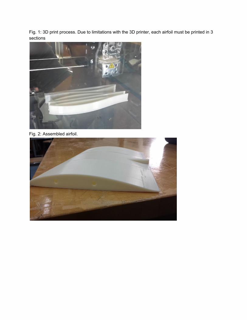
Fig. 1: 3D print process. Due to limitations with the 3D printer, each airfoil must be printed in 3 sections

Fig. 2: Assembled airfoil.

Fig. 3: Bondo applied to surface of airfoil, ready to be sanded smooth

Fig. 4: Hand sanding the surface of the airfoil to uniformity.

Fig. 5: Finished surface of the airfoil. At this stage, gap filler should be used to fill in any remaining imperfections, then sanded smooth.

Fig. 6: The painted airfoils. At this stage, they should be further inspected for surface imperfections and further sanded until the surface is extremely smooth. After repainting, lightly sand all surfaces with 800 grit sandpaper to further smooth the surface

Appendix B: Recommendations for Wind Tunnel Use

Recommendations for Wind Tunnel Use Below are the recommendations, for setting up and testing airfoils in the COE wind tunnel from the 2015­16 Airfoil Modeling Capstone Team. First, we have listed the steps to complete a test on an airfoil per our design. Second, are issues, how they were addressed, and other notes. This information is provided in order to comprehensively show your team the method our team found to prove most accurate and repeatable since this was of significant difficulty in achieving.

I. Comprehensive Steps for Testing For testing, our designed setup includes: The airfoil (3­D printed), sting, the sting mount for the selected angle of attack, two DMMs with alligator clips, allen wrenches of sizes: 3/64”, 5/64”, and 9/64”, and a variety of shims. Step­by­step Test Procedure:

1. Secure the dynamometer to the test section using the 9/64” key, the unit is directional, do not overtighten or at this point fully tighten the screws. The dynamometer should still be able to translate.

2. Attach the sting mount to the dynamometer, using the 5/64”, do not completely tighten yet. 3. Attach the airfoil to the sting mount, using the 3/64” to snug the two set screws. 4. Use a degree level in a few locations (3 along the span works well) to check that the airfoil is

horizontal. Tighten the setscrews fully, so that the airfoil is not able to rotate. 5. Place the level on the flat rectangular portion of the airfoil (directly above the sting protrusion and

check the actual angle of attack of the airfoil. Alter it by placing shims between the dynamometer and the mount about the screw locations. After completing this, the airfoil should be at the exact angle of attack desired, push on the airfoil, in the upstream to downstream direction, to make sure that their is continuous force to displacement (usually this is ensured by placing a shim or two where they will be compressed by the drag force between the mount and the dynamometer).

6. Retighten the sting mount to the dynamometer 7. The spacing between the wing tips and the test section should be very minimal (both tips should

remain within the boundary layer to reduce edge effects). By hand, move the dynamometer base so that the sides of the airfoil are parallel with the test section on both sides, and attempt to keep the clearances equal. For this both the front and rear dynamometer mounting bolts must be loose enough to allow rotation.

8. Then tighten the bolts holding the dynamometer to the test section. These are easily overtightened. When the base can no longer be moved by hand, it is sufficiently tight.

9. Preparations: fasten clasps on top test section wall, open the window of the room and the two doors, connect the dynamometer to the signal box, and connect the leads from this box to the DMM for dc voltage measurement. Barometric pressure and temperature readings are available behind the door between the the wind tunnel and design lab. We used excel to record the data in a format that can be easily processed in Matlab. Alternatively, you could record the forces using LabView.

10. Turn on the signal box and the DMMs, roughly zero the offsets using the wheels on the dynamometer (be sure the set screws are sufficiently tight). RECORD THESE OFFSETS NOW.

11. Use the crank to move the fan away from the test section, ensure there are no loose materials nearby that the fan will intake, you may now turn on the wind tunnel.

12. Increase velocity slowly, closely watching the airfoil for vibrations or deflections. 13. Take measurements from high velocities to low velocities as this proves more accurate than

incrementally increasing the velocity (due to play in the lead screw and the suction forces from the fan).

14. Once the required Reynolds range has be covered, reperform the test from high to low velocities two more times, then turn off the wind tunnel.

15. Once the air has stopped record the final voltage offset. 16. Allow the motor to cool for a 15 minute period prior to restarting.

II. Issues, Solutions, & Notes

1. The necessary equipment is available on the local computer to use labview to record data instead of the meters. We couldn’t get this to work so we used the meters. You will notice that the measurements usually jump around by up to a millivolt, rarely more, usually less, and by watching for a few seconds they indicate a smaller range; the capability with labview to average these jumps would be useful. The airfoil vibrations likely cause the meter readings as they are, they seem to be roughly cyclic fluctuations furthering Note (10). The path of signal filtering could explain translation of the fast airfoil vibrations to the generated output frequency. This may have been a reason our Labview program wasn’t working. A possible counter argument to vibrations being the largest remaining cause of inaccuracy (induced from the fan) is the occurrence during initial offset readings display a manner of this cyclic behavior (usually to a better accuracy than while running). Perplexingly, the final offsets don’t encounter this behavior and usually easily acquire a singular value to the 0.1 millivolt resolution. Reducing or fixing and/or decoupling the fan’s vibrations, along with signal passage are areas of interest.

2. In reducing the presented variables, we would generally take tests on the same day if possible, and change the airfoil before changing the angle of attack.

3. At 2 and 4 degrees forces are significant, so change in AoA and airfoil flex itself is important, as well as being careful at high velocities. Quickly changing a high velocity higher is not advisable.

4. Using the stiffest design (thickest set of flexure plates and steel sting mounts)the signal to noise ratio was found to be poor at low Reynolds. Intuitively, the stiffer flexure plates have a worse signal to noise ratio and are really necessary for the higher forces (above 200,000 Re). With the stiffest plates Airfoil vibration is more apparent at low speeds. With the other plates this vibration occurred, as well as extreme resonance, at high speed. For the range of 200,000 to 450,000 Reynolds, use the stiffest set­up.

5. The airfoils printed should have a minimum wall thickness of 5 mm as well as a sting that extends to the leading edge of the airfoil for extra rigidity. At 2 and 4 degrees this is essential to limit the airfoil body from deforming. A greater wall thickness could be used as long as the plenum extends adequately into the aft section of the airfoil.

6. Occasionally, the final offsets would at times massively change from the initial offsets. One solution is wiggling the connection to the dynamometer; however, the discontinuity will be evident in your data (generally +500 mv in lift or +40­100 mv in drag). A normal change would be ±5­30 mv in either force reading. In this case you take the initial and final point and make a linear interpolation with Reynolds and apply it to the data in MATLAB. If you have a large offset

and the point of change is evident use the offsets separately (although that is not an ideal solution it works well enough, supposing you receive similar normal offset accuracies to what we did).

7. The manometer has a permanent offset of 0.055 inches. It is ideal that one person takes readings from the,manometer using a consistent technique. It also begins to hurt your eyes after a while, I would recommend considering the purchase of a magnifying lense with lighting that could be affixed in front of the manometer, this may help eye strain significantly as well as accuracy of measurement. Another solution is using instrumentation to measure pressure/velocity. Check the path of the pressure taps, that the hoses haven’t come free, or kinked. The tube that connects to the pitot tube, has a tendency to kink near the highest point.

8. Do not apply excessive forces to the dynamometer. Periodically calibrate as necessary. 9. Supposition: Airfoil vibrations in the model mainly come from the fan, since it is not vibrationally

isolated. This vibration adds noise to measurements and accelerates wear on the tunnel. I recommend that you ask for this to be maintenanced or replaced.

10. Dynamometer: In advanced strength of materials Kim Turner talks about how an accelerometer mass doesn't move. Rather, the force necessary to hold this known mass in position (achieved through electromagnets) is how exerted forces are computed. Perhaps this would be a suitable approach.

Appendix C: 2D Passive Bleed & Blow Analysis

Passive Bleed and Blow System Analysis

Winter 2016

Author: Jonathan Prall

12 March 2016

Table of Contents Abstract 1

Background 1

Methods and Procedure 3 Set up and Meshing 3 Investigation of Airfoil Types 6 Agreement With Mathematical Models 8 Two Dimensional Bleed and Blow System Analysis 9

Results and Discussion 10

Conclusion 12

Airfoil Geometry 13

Abstract The purpose of this project was to investigate the effects of a passive bleed and blow­hole system on an airfoil. The driving theory behind the bleed and blow­hole concept is to reduce pressure drag along the upper surface of the airfoil. By allowing air from the higher pressure region to flow into a low pressure region, we expect to see a slight decrease in drag forces. However, this phenomenon may come at the cost of lift and/or increase the overall drag. In order to fully investigate the effects that this system will have on airfoil aerodynamics, physically testing airfoils and comprehensive simulations using COMSOL are being performed. As per our Northrop Grumman sponsor, Phil Barnes, specially designed airfoils with an eight inch chord are being investigated, as compared to a standard NACA0012 airfoil. The optimized airfoils were designed to have a uniform velocity along the upper surface, and a coefficient of pressure that lacks reflex with respect to chord length. By using the SST Turbulence module in COMSOL, we have found that the passive bleed and blow system reduces drag by 50%, but also decreases lift by 20%. The next step is to simulate the system in three dimensions, as the physical system will have spanwise offset holes that cannot be modeled accurately in two dimensions.

Background Aircraft and airfoil design revolves around the idea of minimizing drag and maximizing lift forces to increase efficient use of power during flight time. A passive bleed and blow­hole system, or a system of holes arranged across the top surface of the airfoil, has the potential to accomplish this optimization through air recirculation. We have tested several airfoil designs to investigate potential solutions. Further production, simulation, and physical testing of the airfoils still must be done. A variety of airfoils are to be simulated, 3D printed, finished, and tested in the UCSB wind tunnel by the end of Spring 2016 to explore the phenomenon of a passive bleed and blow­hole system. By Bernoulli’s Equation, when the velocity of a fluid increases, the pressure of the fluid in that region decreases.

This is the fundamental basis for lift generation with airfoils. The shape and angle of attack of an airfoil directs the flow of fluid around it producing a low pressure pocket on the upper surface and increasing the pressure on the bottom surface of the airfoil. By Newton’s third law, this pressure difference exerts a force on the upper and lower surfaces in the same direction, generating lift. As stated previously, the angle of attack and shape of the airfoil drastically alter the flow characteristics around the airfoil. At some angle of attack, known as the critical angle, flow separation of the boundary layer occurs, and the airfoil no longer produces lift. At the critical angle, all of the aerodynamic forces

on the airfoil are drag. Drag is an accumulation forces on the airfoil that are orthogonal to lift, in the same direction as the free stream velocity. The types of drag, as they relate to airfoils, are lift induced drag, caused by vortices and viscous effects, and parasitic drag, caused by surface roughness and pressure effects. Vortex drag is drag induced by the formation of vortices at the tips and

trailing edge of an airfoil where the high pressure fluid on the underside of the airfoil curls around the body, into the low pressure region.

Pressure induced drag is caused by pressure differences along the surface of the airfoil. At high angles of attack, the pressure drag increases as the pressure gradient between the upper and lower surfaces of the airfoil increase. At the critical angle, where flow separation occurs and the airfoil stalls, there is no lift generation and pressure drag increases because of the turbulent, unattached flow on the upper surface.

An airfoil has different pressures around its surface, ranging from "ram" at the stagnation point to strong suction shortly downstream on the upper surface. Also, along the upper surface, strong curvature effects manifest between 40% and 70% chord length at high­lift conditions. The passive bleed and blow airfoils, to be tested in a low­speed wind tunnel, would have a row of holes drilled at some upstream location, with the optimum positioning determined by test, and another row of holes to bleed at 70% chord on the upper surface. Depending on angle of attack and hole location, the bleed and blow­holes will exhibit recirculation which may enhance lift and/or reduce drag at high lift conditions. This is will be done without the need to actively provide high­pressure air as in current systems.

The diagram to the right is a 2D representations of the theoretical bleed and blow system in action, where the arrow symbolizes the flow of air. Although the effects of this system are expected to be in 3D, this figure shows how the air is expected to be drawn through a trailing hole in the high pressure region at 70% chord to the leading hole at 40% chord in the low pressure region. The diagram to the left displays this pressure region that forms along the top and bottom surfaces of the airfoil whilst traveling at subsonic speed.

Methods and Procedure Prior to building and testing an airfoil, a comprehensive analysis was performed using the SST Turbulence module in COMSOL Multiphysics. To analyze each airfoil, a standard model was used that closely approximated the conditions within the UCSB wind tunnel. Pressure distribution graphs, surface velocity charts, and surface pressure charts were plotted for each airfoil. For the bleed and blow­hole analysis, a chart comparing the lift and drag between the clean version of the airfoil and the bleed and blow­hole version were also compared. Set Up and Meshing To streamline the process of simulating several airfoils, a standard model was set up in much the same way as the NACA0012 tutorial in COMSOL. The airfoil was defined by an interpolation curve in the center of a “wind tunnel.” The extents of the wind tunnel are defined by a 90 degree section of a circle and a rectangle, which was then mirrored about the chord line of the airfoil. Finally, the airfoil is subtracted from the wind tunnel to be later defined as a wall.

The radius of the circle and the length of the trailing rectangle must be at least ten times the length of the chord of the airfoil in order to have an accurate solution. This is due to the size of the pressure distribution on the upper surface of the airfoil, especially at greater angles of attack. The table below shows the parameters used in all the simulations performed. Air density and viscosity closely match the UCSB design lab where the wind tunnel is located. The inlet velocity, U_inf, is approximately twice the speed that the wind tunnel is capable of, but corresponds to a Reynolds number of 1,000,000, a more realistic speed for aircraft. The equations for the free stream turbulent kinetic energy and free stream specific dissipation rate also came from the NACA0012 tutorial, and are necessary for the SST Turbulence model.

Parameter Value Description

U_inf 100[m*s^­1] Free­stream velocity

rho_inf 1.19914[kg*m^­3] Free­stream density

mu_inf 1.846e­5[kg*m^­1*s^­1] Free­stream dynamic viscosity

L 0.4[m] Domain reference length

c 203.2[mm] Chord length

k_inf 0.1*mu_inf*U_inf/(rho_inf*L) Free­stream turbulent kinetic energy

om_inf 10*U_inf/L Free­stream specific dissipation rate

alpha 4 Angle of attack

The next plot shows how the model is meshed. A mapped mesh for each of the four domains is created so that the density of elements is greatest around the airfoil as well as behind the trailing edge. Overall, there were less than 100,000 elements in each simulation, giving a good balance between runtime and resolution.

For most of the airfoils, there were 256 elements along the airfoil surface, with approximately 100 boundary layer elements. This high resolution near the airfoil surface allows for the boundary layer to be very well defined, increasing the accuracy of the measurements made on the airfoil surface.

Investigation of Airfoil Types The most important output of these simulations was the Cp vs. Chord % graphs. These graphs plot the non­dimensional pressure coefficient, Cp, along the airfoil surface, x/c, where x is the position along the chord and c is the chord length (8 inches). Cp is defined by the equation below,

/(ρU )1 − p * 2 2 where p is pressure in Pascals, is air density in , and is the free stream velocity in ρ g/mk 3 U2

. The main considerations for candidacy were: large pressure differential across top of/sm airfoil, a smooth decrease and consequent increase in pressure (e.g. no negative pressure spikes), and a uniform pressure distribution along the bottom surface. The graph below shows the pressure distribution along the MOD012 airfoil at angles of attack ranging from 3.5 to 4.75 degrees. It is clear that in this range, the pressure distribution between 0.35 to 0.8 chord % is very large. This makes the MOD012 an ideal candidate for the passive bleed and blow system, as this large pressure difference will drive the system. The second graph plots Cp vs chord percent for the NACA0012 airfoil at angles of attack from 0 to 12 degrees. There

are two reasons that the NACA0012 airfoil is not a good candidate for the bleed and blow system: 1) there is a large pressure spike, the stagnation point, on the leading edge of the airfoil, even at low angles of attack, and 2) the pressure differential between 50% chord and 90% chord is extremely small.

The graph to the right shows the cp vs chord percent graph for the PCS001 airfoil. There is a slight discretization error in the result, due to either the interpolation curve that

defines the geometry introducing flat spots along the airfoil surface, or due to the mesh quality being poor . The pressure 1

differential between

1 After running the simulations a second time with a finer mesh along the surface of the airfoil, the results stayed the same. This leads me to believe that the resolution of the interpolation curve was poor, causing the oscillations in pressure

50% chord and 80% chord is on the order of 0.5, and varies little over small angles of attack. The PCS001 is an ideal candidate for future investigation of the passive bleed and blow system. Like the PCS001, the PCS012 is an ideal candidate for the passive bleed and blow system. The pressure differential between 50% and 75% is ~0.6, making it an even better candidate than the PCS001. The pressure differential between say 40% chord and 85% chord is larger than the pressure differential between 50% and 75% in all cases. The blow hole should not be any closer to the leading edge than 50%, as this is where the flow naturally transitions to turbulence and placing the blow hole further forward than this could result in tripping turbulent flow, increasing drag. The bleed hole cannot be placed much further downstream than 80% as the trailing edge of the airfoils becomes very thin, and the thinner plenum may negate the positive effects of the bleed and blow system by constricting flow.

Agreement With Mathematical Models Our Northrop Grumman sponsor, Phil Barnes, mathematically designed and optimized several airfoils to exhibit this large pressure difference across the upper surface with very little or no reflex at the tail. This is where the pressure on the upper surface exceeds the pressure on the lower surface, depicting a small loop near 90% chord as visible in the graph above. These airfoils are permutations of the PCS012, or Phil’s Cubic Spline 12% chord thickness. Using a mathematical method, he has calculated the expected Cp vs. chord % curve will look like at an optimum angle of attack. The three plots below compare the mathematical models of the airfoils in red, and the computationally determined Cp in blue.

It is clear that the computational model of the PCS012 matches the mathematical model very closely, while the PCS012A and PCS012B results match the general trend of the mathematical models, but with slight error. Since our PCS012 model matches the mathematical results the best, we decided to move forward with that airfoil for future simulations and physical testing.

Two Dimensional Bleed and Blow System Analysis

In order to determine the effects of the bleed and blow system in two dimensions, a more comprehensive simulation of the PCS012 airfoil was performed. The two dimensional simulation of the bleed and blow system is not perfect, as the bleed and blow holes are now representative of slots cut into the wing spanwise. This causes a level of inaccuracy in the results, as the bleed and blow system is expected to be a three dimensional phenomenon. Therefore, the following results should be viewed taking this into account, and more accurate computational analysis will need to be three dimensional. The table below shows the variables used in the simulation . The 2

upstream pressure is used to define the pressure at the downstream hole and visa versa. The variables Lift2 and Drag2 find the overall force in the Y and X directions respectively using the stresses at the wall, a function only found in the SST Turbulence module. The lift and drag variables are used solely in the analysis

Variable Definition Description

p_upstream2 aveop2(p2) pressure at bleed hole

p_downstream2 aveop1(p2) pressure at blow hole

Lift2 intop1(spf2.T_stressx*sin(alpha*pi/180)­spf2.T_stressy*cos(alpha*pi/180)) Total force of lift

Drag2 intop1(­spf2.T_stressy*sin(alpha*pi/180)­spf2.T_stressx*cos(alpha*pi/180)) Total force of drag

The two figures below show the velocity magnitude around the PCS012 at an angle of attack of eight degrees. The first figure shows the clean airfoil, with boundary layer separation occurring at approximately 70% chord. This boundary layer separation is typical of airfoils at higher angles of attack, or where there is dramatic convex curvature of the trailing surface. At the critical angle of attack, the boundary layer

2 The pressure boundary conditions do not account for mass flow, increasing the error significantly. In the next iterations of this simulation there will be a mass flow constraint on the bleed and blow holes.

separates very close to the leading edge of the airfoil, drastically increasing pressure induced drag, and reducing lift to nearly zero. In general, turbulent flow and boundary layer separation increase the skin friction drag along the airfoil. For comparison, the figure to the right shows the PCS012 airfoil under the same flow conditions, but with the passive bleed and blow system in place. Note the lack of boundary layer separation at the trailing edge and the large low velocity pocket immediately downstream of the airfoil. Even if the bleed and blow system does not equalize the pressure along the upper surface as intended, the effects of delaying or eliminating boundary layer separation will, in theory, reduce skin friction drag overall.

Results and Discussion

Initial comparisons of the drag coefficient between the clean and bleed and blow airfoil are promising. The drag coefficient at angles of attack between zero and eight degrees for the bleed and blow airfoil show a 50% reduction when compared to the clean airfoil.

where is the overall force of drag and is in degrees/(ρ ) Cd = 2*Fd *U

2* c Fd α

However, the bleed and blow airfoil also reduces the total lift generated, compared to the clean airfoil, on the order of a 20% reduction. While this is not ideal, the decrease in drag is twice as

large as the decrease in lift, meaning that this system may still exhibit an overall increase in airfoil efficiency.

where is the overall force of lift/(ρ ) CL = 2*FL *U

2* c FL

Both and were measured using the normalized viscous stress in the x and y­direction F d F L respectively. This is where the SST turbulence model excels, as high wall resolution increases the accuracy of the measurement of viscous stress along walls. The vs. chord % graphs for both the clean and bleed and blow PCS012 airfoils clearly exhibit Cp error in the computational analysis. The curve for the clean airfoil, shown in the plot below, is relatively smooth, with the exception of the sharp pressure spikes near the trailing edge of the airfoil. Even with this discrepancy, the vs. chord % graph for the clean PCS012 closely Cp matches that of previous two dimensional simulations.

The vs. chord % graph for the bleed and blow PCS012 airfoil is also very uniform, with the Cp exception of the pressure spikes at the bleed and blow locations. This is an artifact of the boundary conditions imposed at the bleed and blow­hole locations and introduces additional error to the solution. Even with these artifacts present, it is clear that the bleed and blow system decreases the pressure between 0 and 50 % chord and increases the pressure between 50 % and 75% chord. The smoothing of pressure along the lower surface of the airfoil is the exact effect that we were hoping to accomplish.

Conclusion After numerous simulations, and many hours of troubleshooting, the passive bleed and blow system has been found to be capable of reducing drag at the cost of lift. The “slot” geometry used in the two dimensional simulation resulted in a 50% decrease in drag and a 20% decrease in lift, as well as a smoother pressure distribution along the upper surface of the airfoil at moderate speeds. For future investigation, a mass flow condition needs to be placed on the inlet and outlets for the bleed and blow holes as the system is passive. Future exploration of the passive bleed and blow concept will need to be three dimensional to properly model the bleed and blow holes as holes, and to offset them in a grid pattern along the airfoil surface. We have already seen that the effects of the bleed and blow system are quite small, but not insignificant; therefore, the accuracy of future models needs to be much greater, meaning that most of the investigation will be with low speed, laminar flow. The turbulence conditions are extremely difficult to have work properly, with little error, and in three dimensions these effects will astronomically more difficult.

Airfoil Geometry PCS001 Airfoil

X Z 0.9999986732 ­0.0013000717 0.8354042388 ­0.0096975921 0.6752995401 ­0.0159466083 0.3857866811 ­0.0199645802 0.1628332544 ­0.0198881959 0.0305996826 ­0.0137250237 2.77555756156289E­017 0 0.03180952750.0304555469 0.07032459940.0461144025 0.18470894430.0759715804 0.33313243560.0962708076 0.49376470910.098373528 0.64588425350.0815938829 0.77438240320.0546448557 0.87281721180.0291631169 0.94429710750.0118283966 0.99999957540.0013000749 0.99999957540.0013000749 0.77438240320.0546448557 0.87281721180.0291631169 0.94429710750.0118283966 0.99999957540.0013000749

PCS012 Airfoil

X Z 0.9999986732 ­0.0013000717 0.8354042388 ­0.0096975921 0.6752995401 ­0.0159466083 0.3857866811 ­0.0199645802 0.1628332544 ­0.0198881959 0.0305996826 ­0.0137250237 2.77555756156289E­017 0 0.03180952750.0304555469 0.07032459940.0461144025 0.18470894430.0759715804 0.33313243560.0962708076 0.49376470910.098373528 0.64588425350.0815938829 0.77438240320.0546448557 0.87281721180.0291631169 0.94429710750.0118283966 0.99999957540.0013000749 0.99999957540.0013000749 0.77438240320.0546448557 0.87281721180.0291631169 0.94429710750.0118283966 0.99999957540.0013000749

PCS012A Airfoil

X Z 0.9999986732 ­0.0013000717 0.8354042388 ­0.0096 0.6752995401 ­0.014 0.3857866811 ­0.0199645802 0.1628332544 ­0.0198881959 0.0305996826 ­0.0137250237 2.77555756156289E­017 0 0.03180952750.0304555469 0.07032459940.04731 0.18470894430.0773 0.33313243560.0962708076 0.49376470910.098373528 0.64588425350.0815938829 0.77438240320.0546448557 0.87281721180.0291631169 0.94429710750.0118283966 0.99999957540.0013000749 0.99999957540.0013000749 0.77438240320.0546448557 0.87281721180.0291631169 0.94429710750.0118283966 0.99999957540.0013000749

PCS012B Airfoil

X Z 0.9999986732 ­0.0013000717 0.8354042388 ­0.0094 0.6752995401 ­0.0135 0.3857866811 ­0.0199645802 0.1628332544 ­0.0198881959 0.0305996826 ­0.0137250237 2.77555756156289E­017 0 0.03180952750.0299 0.07032459940.04761 0.18470894430.08 0.33313243560.1002 0.49376470910.101 0.64588425350.0815938829 0.77438240320.0546448557 0.87281721180.0291631169 0.94429710750.0118283966 0.99999957540.0013000749 0.99999957540.0013000749 0.77438240320.0546448557 0.87281721180.0291631169 0.94429710750.0118283966 0.99999957540.0013000749

Appendix D: Investigation of Hole Geometry in 2D

COMSOLFinalReport:_____________________________

!!!!Inves7ga7onofHoleGeometriesforuseinaPassiveAirfoilBleedandBlow

System!

_____________________________

!!

CreatedBy:MichaelRubin

!Date:

3/11/16

2

!!TableofContents!

1. Abstract…………………………………………………………………………………………………………………..……2!2. Background……………………………………………………………………………..…………………………….…….2!3. MethodofSimula7on…………………………………………………………………………………………………5

3.1. FirstSimula7on:PCS0012AirfoilinWindTunnel………………………………………………53.2. MainSimula7on:HoleGeometryInves7ga7on……………………………………………………8!

4. ResultsandDiscussion…………………………………………………………………………………………….…114.1. FirstSimula7on:PCS0012AirfoilinWindTunnel………………………………………………114.2.MainSimula7on:HoleGeometryInves7ga7on…………………………………………………15!

5. Conclusion………………………………………………………………………………………………………………….19!!!!!!!!!!!!!!!!

2

1.Abstract:ThePurposeofthisreportistoinves7gatetheextentoftheeffectsofvariousholegeometriesonthefluidflowwhichpassesthroughthem.Threeholetypesareconsidered:adrilledhole,achamfered hole, and a filleted hole. Fluid flow is induced by a pressure differen7al which isderived from a separate airfoil COMSOL simula7on. These pressure differen7als are directlyfromthepressurefoundalongthetopsurfaceoftheairfoilbeingmodeledatloca7onsof40%chord and 70% chord. A set of four surface pressures are calculated corresponding to airfoilanglesofa^ack,AoA,of0°,2°,4°,and6°.Theholesthemselvessitnormaltothelengthofthechord and are connected through a reservoir body, referred to as the plenum, whichgeometricallyresemblestheplenumofthephysicalmodel.!Theholeshaveadiameterof0.1inchesandalengthof0.2inches.Duetothisrela7velyshortlength,entranceeffectsareexpectedtobesignificant.Nonetheless,computa7onofvolumetricflowratesconsistently supportedFluiddynamics theoriesand revealed that thefilletedholesbestallowedtheflowpassage,closelyfollowedbythechamferedholegeometry.Leastefficientwas the simple drilled hole geometry due to the sharp bend angles the fluid flow had toincorporate. The filleted hole allowed to pass 2.54 7mesmore fluid volumetrically than thesimplydrilledhole.Thechamferedholepassed2.057mesmorefluidvolumetrically than thedrilledhole.!2.Background:This inves7ga7on isbeingperformedfordirectpurposeforaCapstoneProject.Thisproject issponsored byNorthropGrumman, a global defense and aerospace company. The immediatepersonal sponsor to the project is Phil Barnes,who has theorized, aswell asmathema7callydemonstratedthatthelidtodragra7oofcertainairfoilscanbeincreasedbyuseofapassivebleedandblowsystem.

Figure 1 illustrates the system in 2-D format. The passive bleed and blow system takesadvantageofthepressuredifferen7alacrossthetopsurfaceofanairfoil.Astaggeredmatrixofholes are strategically placed along this surface at specific loca7ons that seemmost likely atmaximizing the flow through this system. These loca7ons are airfoil specific. The holes are

16

Figure 1: Airfoil with incorporated Passive Bleed and Blow System.

2

placedinastaggeredforma7onrela7vetotheflowdirec7oninordertonotsimplyrecirculatethe “blown” air back through the “bleed” hole, but instead, counter rota7ng vor7ces areallowed to form along the airfoil surface downstream of the blow holes. These vor7ces areexpectedtohelp(slightly)increasethelidforceoftheairfoil.Inaddi7on,thedragforceoftheairfoilshouldbereducedsincepressurealongitssurfaceisequalized,tosomeextent,allowingfortheflowtopassovereasier(i.efaster).Thusthepassivebleedandblowsystemisexpectedtoincreaselidforcewhiledecreasing thedragforce,yieldingahigherlidtodragra7o.Shouldthiswork,itwouldbequiteanadvancement,mostapplicabletosmallunmannedaircrad.ThelikelyrangeofbeneficeisfromaReynold’snumberof200,000to2,000,000.Reynoldsnumberisanon-dimensionalvaluethat, throughsimilitude, isusedtopredictsimilarity inflowpa^ernsfordifferentfluidflowsitua7ons.Itcorrelatestheeffectsofatestairfoilinwindtunneltes7ngtotheeffectsencounteredinrealflight.Itisthera7oofiner7alforcestoviscousforcesofafluidandisprovidedasEqua7on1.!!Thevariablesof Equa7on1are:fluiddensity,, flowvelocity,V, characteris7c length,L,andfluidviscosity,μ.Reynold’snumberiscalculatedperhapsmostoftentodeterminethepositionalong the characteristicwhere a flow transitions from laminar to turbulent. Both simulationshaveturbulentflow.Thecharacteristiclengthfortheairfoilsimulationisthechordlength,andtheholediameterfortheholegeometrysimulation.!The most promising candidate airfoil thus far is the PCS 0012. This is a non-standard,asymmetric,airfoilcreatedbyacubicsplinemethod(PCSstandsforPhil’sCubicSpline).Ithasaparametric curve, and thus its geometry is easily importable into simula7on programs likeCOMSOL. Keeping in naming conven7onof airfoils, the 0012denotes a thickness of 12% thechordlength,measuredatitsthickestpoint.Parametersusedinthe twosimula7onsoriginate

16

Figure 2: Common airfoil terminology.

(1)

3

from the Capstone project. Figure 2 is shown as a guide for terms used to describe airfoils.Chordlengthis8 inches.Holesizesare0.1inchesindiameter.Anglesofa^ackof interestare0-6°,with4°themostpromisingtodemonstratetheeffectsofthisbleedandblowsystem.!Both simula7ons u7lize the Navier-Stokes equa7on for fluid mo7on since they are bothturbulentflowsimula7onsusingstandardair.ThisisshownbelowasEqua7on2.

Theairfoilsimula7onaddscomplexitybyaddingcompressibleflowtermstotheNavier-Stokesequa7onsincetheflowisconsideredcompressible.ThisexpandedversionisshownasEqua7on3.Thecon7nuityequa7on,Equa7on4,isalsousedinunisonwiththeNavier-StokesEqua7onsin both simula7ons. Equa7on 2, from led to right is iner7a per volume, pressure gradient,viscosity,andotherbodyforces.

The airfoils themselves are 3-D printed at UCSB and are hollow. Aderwards, they undergo alengthysurfacefinishingprocess.Thentheyarereadytobephysicallytestedinthewindtunnel.This report looks at the extent of benefit to the internal flow that a more complex holegeometrywouldhaveduetothelevelofdifficultyinactuallycrea7ngafilletorchamferontheinsideof theassembledairfoils.The3-Dprinter isnotcapableofdoingthis,leavingthebestsolu7onto cut the bo^om surface off, and create thechamferorfilletbyhand,andreplacethebo^om.This has two problems. It would be a difficult,delicate, and 7me consuming task to achieve.Secondly, this process would become arepeatabilityissue,asitwouldbehardtocuteachairfoilthesameway,todigouttheholes,smooththem,andthenreplacethebo^omsec7ontobeperfectly flush again. Due to this process beinghard to replicate on each of our test airfoils, andwindtunneltestrepeatabilityamajorconcernfortheprojectsponsor,theresultsshowninthisreportwillhave tobeweighedagainst thechallengeof integra7ng theholegeometryon theairfoilwithinthescopeoftheproject.

16

(3)

(2)

(4)

Figure 3: 3-D printed and finished PCS 0012.

4

3.MethodofSimula7on:COMSOL 5.2 was the program used for the simula7ons. While this report is about holegeometry forfluidtopass through, thefirststepwastomeasurethepressuredifferen7alsattheholeloca7onsthatwoulddrivethefluidflow.Thesewerefoundviatheairfoilsimula7on.!3.1.AirfoilSimula7on:Thisisdonebysimula7onofthePCS0012airfoilsubjectedtoairflowof50m/s.Thesimula7onsweeps throughanglesofa^ackof0-6°, theseare theanglesofa^ack thatwillbephysicallytested.Awindspeedof50m/sisusedsinceitiswhatthewindtunneloncampuscanachieve.

!ThePCS0012parametriccurveisusedtobuildaninterpolatedopencurveinCOMSOL,whichisthenrenderedintoasolid.Thisisscaleddowntobethesamesizeasthephysicalmodelsbeingused.Above,Figure4isofthePCS0012airfoil,theaxisareinmeters.Thechordlengthisvisibly.2032meterswhichisequalto8inches.!Theairfoil solid issubtractedfromthewindtunnelgeometry,which iscreatedbymirroringaquartercircleandarectangleaboutthey-axis.Theairfoilposi7onisvisibleatthecenterofthecirclewhichcomprisesthe ledsideof thewindtunnel.Airflowtravels fromledtoright.The

16

Figure 4: Interpolated curve for PCS 0012.

5

bluelineinFigure5istheflowinletandtheanopenboundaryallowsforthefluidtoescapeouttherightside.Wallcondi7onsareascribedtotheemptyspacethatistheairfoiltocreatearigidobstaclefortheflowtopassaround.Theproper7esofairarephysicscontrolledfromthebuiltinmaterial.

Averyfinecustommappedmesh isbuilt inordertocaptureaccurateresults.Figure6showsthe en7rety of themeshed domain. Figure 7 is a close-up of the surroundings of the airfoilsurface.Figure7be^erillustratesthereasoningbehindhowthemeshisbuilt.Inordertohavehighaccuracyat the leadingedge,airfoil surfaceandtrailingedge,where intricateflowdetailoccurs,distribu7onsovertheseareasarespecified,alongwithboundarylayersinthoseareas.Figures8-10showthemeshqualityaroundtheseimportantareas.

16

Figure 5: Airfoil geometry subtracted from the wind tunnel.

Figure 6: Meshed domain. Figure 7: Mesh close-up around airfoil.

6

Thesimula7onisrunusingtheSSTturbulentmodel.TheSSTmodelwaschosenasitisoneofthemost accurate turbulentflow solvers, best suited forflownearwalls,which is theairfoil.Whiletheflowof50m/sisbelowtheaircompressibilitystandard0.3machspeed(about0.145mach),thereisacertainamountofcontribu7onthatcanbeaccountedforbyconsideringtheflowtobecompressibletoadegree,sothisisdoneaswell.

16

Figure 8: Mesh quality around airfoil.

Figure 9: Mesh quality about the leading edge. Figure 8: Mesh quality about the trailing edge.

7

!3.2.HoleGeometrySimula7on:This simula7on is the purpose of this report. The goal is to find rela7ve efficacy in u7lizingchamferedorfilletedholesinthepassivebleedandblowsysteminplaceofastandard,simple,drilled hole. The effec7veness of these geometries will be compared by measurement ofvolumetricflowratesofthefluidflowforeachpressuredifferen7al.!This simula7on decouples the flow external of the airfoil to that internal of the airfoil. Thissimplifies the model tremendously. While this simplifica7on may lead to less accuratevolumetricflowratesfromthepressureinducedflowthanwhat isexpected, its7llservesthecompara7vepurposesbetweengeometries.Sinceinternalflowwillnotaffectexternalflow,theholesnolongerneedtobestaggeredandthesimula7onmaybecompressedto2-D.!Asdonepreviously,aninterpola7oncurvewasusedtobuildthePCS0012geometry.Thiswasrenderedintoasolid.Next,ascalingopera7onwasusedtobuildanotherPCS0012curve,butsmallerinbothdimensions,thiswasalsorenderedintoasolid.Thescaledsolidwassubtractedfrom the larger solid in order to create thickness in the curve. This thickness is that of thephysicalairfoil.Figure11showstheresultsofthis,theunitsareininches.

16

Figure 11: PCS 0012 given thickness.

8

Thefinalmajorsimplifica7onwastoapproximatethehollowedinternalgeometryoftheairfoil,theplenumofFigure11,asanellipse.ThissimplifiedgeometryisshowedinFigure12.Bothareapproximately 7 inches along the major diameter and 0.75 inches across the minor. Incomparing Figure 11 and Figure 12, the similarity of the shape is evident. Especially whenconsideringflowwillonlybepassingthroughbetween40-70%ofthelength

Theholesarethenplacedattheirrespec7vechordposi7ons.Thedrilledholesaremodeledin2-D as rectangles. The chamfer andfillet opera7ons are used tomake the other geometries.Figures13and14showthechamferedholeandthefilletedholerespec7vely.Theseholeshaveatopandbo^omtwicethewidth(diameterin3-D)ofthemidsec7onandthedrilledhole.Theholefartherdownthechordlengthisintheposi7onofhigherpressureandthereforeservesas

16

Figure 12: Simplified plenum geometry.

Figure 13: Chamfered hole. Figure 14: Filleted hole.

9

the inlet. Theupstreamhole is theoutlet. Everythingelse is consideredawallwithano slipcondi7on.Thetopoftheholegeometryistheoutersurfaceoftheairfoil,whichiswhytheycanbeplaceduponthetopofthesimplifiedgeometry.!Ini7alresultsshowedtheexpectedreturnthatthejetofairflowfrominlettooutletwouldberetainedbetweenthetwo.Acustommeshwascreatedwherethefirst30%ofthechordwouldhaveacoursemeshinordertocutdownoncomputa7on7me,andthisworkedtoanextent.Therightsidefreetriangularmeshwassettoextrafine.Thismeshalsouses10boundarylayersaswellasrefinementaroundcornersmostcri7caltotheflow.Below,Figure14showstheen7remeshed domain. Figure 15 illustrates the corner refinement aswell as the par77on ofmeshquality.

16

Figure 15: Corner refinement of custom mesh.

Figure 14: Custom mesh (shown with drilled hole geometry.

10

!4.ResultsandDiscussion:Thissec7onofthereportwillbeginwiththeresultsoftheairfoilsimula7on,andthenmovetothat of the hole geometry inves7ga7on, as well as a discussion of the results of the holesimula7on.!4.1.AirfoilSimula7onResultsandDiscussionThesimula7onresultswereusedtoplotstreamlinevelocityfieldsaswellaspressurecontoursacross theairfoil surface.Figures16andFigure17showthestreamlineveloci7es for thefirstand last angle of a^acks swept through for comparison purposes. Of note is that the free-streamvelocity inbothis50m/s,whichistobeexpected,andcanbediscernedviathecolorlegendontherightofthefigures.Thefasterairvelocitytravelingoverthetopoftheairfoil isvisible inred inbothfigures. Increasingtheangleofa^ackshidsthisdistribu7ontowardsthenoseoftheairfoil.ThiswillalsobeshowninthepressurecontoursinFigures18and19.Thesedisplayrela7vepressurechangesaroundtheairfoilsurfaceinunitsofpascals.

16

Figure 16: Velocity streamlines around airfoil with 0° AoA. Values in

11

16

Figure 17: Velocity streamlines around airfoil with 6° AoA. Values in m/s.

Figure 18: Pressure contour for 0° AoA. Figure 19: Pressure contour for 6° AoA.

12

!!Theabovefourfiguresshowvelocitystreamlinesandpressurecontoursatanglesofa^acksof0°and6°.Thesetwoextremesarechosenfordemonstra7onpurposes,theintermediateanglesare well placed within this trend. Comparing the velocity and pressure figures for 0° makesevidenthowthe lowspeedsmatchwithhighpressure (noseandtail) regions.Comparingthedifferentanglesofa^ack,theshidinthehighspeed,lowpressureareaisdis7nct.Byincreasingtheangleofa^ackoftheairfoil thestagna7onpoint,highestpressureshown inred,shidstobelowtheleadingedgeandredistributestheimmediatelowpressureregiontonolongerbeoneitherside,as inthe0°AoA,butonthetopofthe leadingedge.ThecontoursonthetrailingedgeinFigure19indicatesflowsepara7on.!Forthepurposesofthisreporttheholeplacementmustbevalidated,aswellasthepressuresat those points be found. Figure 20 is a standard plot showing the pressure coefficient, Cp,acrosstheuni7zedairfoilchordlength,x/c,wherexdenotesposi7onandcisthechordlength.Themul7plelinescorrespondtothemul7pleanglesofa^ack.

Cp isdefinedperEqua7on5,whereP ispressure,U is free-streamvelocityand is the free-stream density. Per Equa7on 5, Figures 20 and 21 will display propor7onal trends since thecoefficientofpressureislinearlydeterminedfromthepressure.

16

(5)

Figure 20: Cp versus chord length.

13

Now thepressure itself, inpascals, is plo^edalong the same length, Figure21. Thepressurevaluesatchordlengthsof40%and70%arenotedforeachangleofa^ack.

These four sets of pressure values are the values needed simulate theflow likely to be seenthroughthepassivebleedandblowsystem.Thedifferenceinpressuresbetweenthetwochordposi7ons is reduced toaΔP,apressuredifferen7al,which is appliedat the inletof theholesbeingconsidered,andtheoutletwillhaveapressureofzero.Table1displaystheseresults.

!

16

Table 1: Results from airfoil simulation used to drive airflow through the holes of the second simulation.

Figure 21: Relative pressure versus chord.

14

4.2.HoleGeometrySimula7onResultsandDiscussionThesimula7onresultsaremosteffec7velyrenderedasvelocityplots.Velocityflowstreamlineswerealsoaddedinordertogiveanideaofthemo7onoutsideoftheflowstreamthatoccurreddotothegeometryofthereservoir itpassedthrough.Eachofthefourpressuredifferen7als,fromtheresultsinTable1,wereappliedtotheinlet,the70%chordhole(theoneontheright).Figures22-28showtheseplots forthesmallestand largestpressuredifferen7al foreachholegeometry.Axisvaluesareinm/s.

16

Figure 22: Drilled hole with 1st ΔP of Table 1.

Figure 23: Drilled hole with 1st ΔP of Table 1 with velocity magnitude lines.

Figure 24: Drilled hole with 4th ΔP of Table 1.

15

The above figures illustrates the passage of themain flow. This reveals the importance of achamferedorfilletedholeversus thedrilledholebecause theflowdoesnot thenneedbendaroundsucha sharpcorner.Allowing theflowto take themostdirect route isalsobeneficialsince increases in ΔP applied visibly increase the eddy currents. Close-ups of the outlet areshowninFigures29-32below.!

16

Figure 25: Chamfered hole with 1st ΔP of Table 1.

Figure 26: Chamfered hole with 4th ΔP of Table 1.

Figure 27: Filleted hole with 1st ΔP of Table 1.

Figure 28: Filleted hole with 4th ΔP of Table 1.

Figure 29 shows the difficulty the flow encounters to exit at such a bend. Boundary layersepara7on occurs along the right wall. As a result there is amaximum velocity through theoutletupwardsof50m/s,wheretoitsrightisonly10m/s.Theoutletofthechamferedhole,Figure30,showsthisaswell,however,theboundarylayersepara7onismuchsmallerfromtherightwall.Thechamferalsoallowsfortheflowthroughtheoutlettobeexi7ngver7cally,whilethedrilledholedoesnot.Theul7matesolu7ontotheseissuesisthefilletedholeofFigures31and32.Heretheboundarylayeristhesmallest.Themaximumvelocityisapproximately45m/sandthefilletbendismuchmoreappropriateforthespeedofthefluidflowtoreasonablybendaroundandenter.Thisiseasilyno7cedinthedirec7onlinesofFigure32.Anevenmoregradualfilletwouldseembeneficial.!

16

Figure 29: Drilled outlet hole with 4th ΔP of Table 1.

Figure 30: Chamfered outlet hole with 4th ΔP of Table 1.

Figure 31: Filleted outlet hole with 4th ΔP of Table 1.

Figure 32: Filleted outlet hole with 4th ΔP of Table 1 and velocity stream lines.

17

!!!!!!!!!!!!!

!!!!!!!!!!!!!!

16

Bymeasuring theaveragevelocityacross theoutletandmul7plying that valueby thecrosssec7onalarea(3-Dvalue)thevolumetricflowratesweremeasuredforeverycombina7onofpressureandholegeometry.Thegoalistomaximizetheflowrate.Atthis,thefilletedholeissuperior.Thefollowingfigures,Figures33and34showlinegraphsofthevolumetricflowratesat each pressure for the different geometries. Figure 34 normalizes the flow rates of the

Figure 33: Volumetric flow rates of each hole geometry at each ΔP.

Figure 34: Normalized Volumetric flow rates at each ΔP value.

Drilled

18

Theaveragevelocityprovedtoincreasepropor7onallytotheincreaseinpressure.Thussodoesvolumetricflowrate.WhilethiscanbeunderstoodfromeitherFigure33orFigure34,inFigure34thenormalizedvaluesareveryclosetoflatlines,provingpropor7onality.!Figure 34 displays the crucial return that this report has been progressing towards. Incomparisontosimplydrillingholesforthepassivebleedandblowsystem,bothchamferedandfilleted holes excel in augmen7ng the flow rate. Taking the mean values of the normalizedcurvesofFigure34gavetheresult that thevolumetricflowrate throughachamferedhole is2.057meshigher,andthatofthefilletedholewas2.547meshigher,comparedtothedrilledhole. Also to note, these numbers are accurate across the range of pressures that will beimposedontheairfoil!5.Conclusion:As an7cipated, the filleted hole outperforms the chamfered and the drilled hole. Theperspec7ve thatFigure34gives is that thedifferencebetweentheflowratesofachamferedhole to a drilled hole is a step certainly worth taking. Whether or not the lesser increaseobtainedfromexchangingachamferedhole forafilletedhole isworthwillbediscussedwiththeprojectsponsor. It is likelythatthereturnofafilletedholeoverachamferedholeforthepassivebleedandblowsystemwillnotbedeemedworthitfortheaforemen7onedreasonsofthepossiblyforsakingrepeatabilityandthedifferenceinproduc7on7me.Unlessarepeatablemethodofcrea7ngasmoothedfilletedholeisfound,theairfoilswillmorethanlikelyusethechamferedholegeometryforthepassivebleedandblowsystem.Achamferedholeisamuchsimpler opera7on to produce and a^ains 80.7%of the flow rate increase that a filleted holewouldprovide.

1619