Passive Air Samplers for Semivolatile Organic …...ii Passive Air Samplers for Semivolatile Organic Compounds: Experiments, Modeling, and Field Application Xianming Zhang Doctor of

Passive Air Samplers for Semivolatile Organic Compounds: Experiments, Modeling, and Field Application

by

Xianming Zhang

A thesis submitted in conformity with the requirements for the degree of Doctor of Philosophy

Department of Chemistry University of Toronto

© Copyright by Xianming Zhang 2012

ii

Passive Air Samplers for Semivolatile Organic Compounds:

Experiments, Modeling, and Field Application

Xianming Zhang

Doctor of Philosophy

Department of Chemistry

University of Toronto

2012

Abstract

Knowledge gaps related to mass transfer processes involved in passive air sampling of

semivolatile organic compounds and factors potentially influencing passive sampling rates

(PSRs) were addressed with controlled laboratory experiments, mass transfer modeling, and a

field sampling campaign. The observed non-uniform SVOC distributions within porous passive

sampling media (PSMs) contradict an assumption in an earlier passive air sampling theory and

proved the existence of a kinetic resistance on the PSM side. This resistance can affect PSRs as

revealed by a new PAS model which is based on fundamental laws of mass transfer in air and

porous media. By considering mass transfer processes within the PSM, the model is able to

explain the large variations of field calibrated PSRs with temperature and between SVOC species

and the two-stage uptake process, which cannot be addressed by the earlier PAS theory. Because

the PSM side kinetic resistance invalidates the assumption that depuration compounds added to

the PSM prior to deployment are subject to the same kinetic resistance as the sampled SVOCs,

PSRs derived from the loss rates of depuration compounds can differ from the actual PSRs of the

sampled SVOCs. Using such PSRs could thus introduce additional uncertainty to PAS-derived

air concentrations.

iii

Experiments using XAD-resin and silica-gel filled mesh cylinder as PSMs for the uptake of

SVOCs and water vapor respectively revealed that sorbent in the inner portion of the PSM does

not take part in chemical uptake; PSRs are thus proportional to the interfacial transfer area but

not the amount of the sorbent. Accordingly, thinner PSM can be used to reduce the amount of

sorbent while keeping or even increasing the PSRs. Optimized designs of PASs could be tested

time efficiently using the gravimetrical approach based on water vapor uptake by silica gel.

iv

Acknowledgments

First, I would like to express my sincere gratitude to my supervisor, Prof. Frank Wania, for his

continuous support during my PhD study. His deep insight and innovative ideas in the field of

environmental chemistry have been guiding me throughout my PhD. I also thank Ying Lei for

the guidance and assistance in the lab. I would like to thank my supervisory/exam committee

members, Profs. Terry Bidleman, Miriam Diamond, Jennifer Murphy and Eric Reiner for their

guidance during my PhD study, and Prof. Thomas Holsen (Clarkson University) for being part of

my defense committee.

Thanks also go to the collaborators in my PhD research projects: Dr. Takeshi Nakano and

Masahiro Tsurukawa (Hyogo Prefecture Institute of Environmental Sciences, Japan), Prof. Akira

Kondo (Osaka University, Japan), and Dr. John Barnes (Mauna Loa Observatory, USA). I

appreciate the collaborations with you. Without these collaborations, the accomplishments I’ve

made during my PhD study would not have been possible. I also thank Prof. Kai-Uwe Goss

(Helmholtz-Centre for Environmental Research–UFZ, Germany), Dr. Eldbjørg Heimstad

(Norwegian Institute for Air Research–NILU, Norway), Dr. Li Shen, Dr. Satyendra Bhavsar

(Ontario Ministry of Environment), and Ingjerd Krogseth (NILU) for the opportunities to work

together on some projects beyond this thesis.

I would like to thank my colleagues in the Wania Group–Dr. Jon Arnot, Dr. James Armitage, Dr.

Trevor Brown, Anya Gawor, Johnny Westgate, Cristina Quinn, Dr. Hang Xiao, Dr. Chuba

Shunthirasingham, Dr. Steve Hayward and summer students – Cindy Wong and Xiaoshu Cao for

different types of assistance during my PhD.

I am gratitude to the graduate student advisors Ms. Anna Liza Villavelez and Ms. Denise Ing at

the Department of Chemistry and Mr. Pavel Pripa at the Centre for Environment, for their help

during my PhD.

I would like to acknowledge the Graduate Student Award from the Centre for Global Change

Sciences (University of Toronto) for supporting my field work; the Ontario Graduate Scholarship

for financial support; travel fellowships for me to attend conferences by the Department of

Chemistry, Faculty of Arts and Sciences and School of Graduate Studies, University of Toronto

Finally, I extend my thanks to my family and friends, who have always been there providing

continuous support and encouragement.

v

Table of Contents

Acknowledgments .......................................................................................................................... iv

Table of Contents ............................................................................................................................ v

List of Tables ................................................................................................................................ xi

List of Figures .............................................................................................................................. xiii

List of Acronyms .......................................................................................................................... xx

Chapter 1. Passive Air Samplers for Semivolatile Organic Compounds: An Overview ................ 1

1.1 A Historical Perspective on the Development of Passive Air Sampling Techniques ......... 1

1.2 Applications of Passive Air Samplers for SVOCs .............................................................. 5

1.3 Mechanism and Theory of Passive Air Sampling ............................................................... 7

1.4 Factors Influencing Passive Air Sampling Rates .............................................................. 11

1.5 Objective and Structure of the Thesis ............................................................................... 14

Chapter 2. Sampling Medium Side Resistance to Uptake of Semi-volatile Organic Compounds

in Passive Air Samplers ........................................................................................... 16

2.1 Abstract ............................................................................................................................. 17

2.2 Introduction ....................................................................................................................... 17

2.3 Materials and Methods ...................................................................................................... 19

2.3.1 Passive Sampling Media. ...................................................................................... 19

2.3.2 Chemicals. ............................................................................................................. 20

2.3.3 Sampling Design. .................................................................................................. 20

2.3.4 Sample Extraction and Analysis. .......................................................................... 21

2.3.5 QA/QC. ................................................................................................................. 22

2.3.6 Derivation of passive air sampling rates. .............................................................. 22

2.3.7 Derivation of the effective diffusivities on the PSM side. .................................... 22

2.3.8 Mechanistic model of effective diffusivity in porous media. ............................... 23

2.4 Results and Discussion ..................................................................................................... 23

vi

2.4.1 Passive Air Sampling Rates. ................................................................................. 23

2.4.2 Evidence of kinetic resistance on chemical transfer within PSM. ........................ 25

2.4.2.1 PCB Uptake from Air. ............................................................................ 25

2.4.2.2 Depuration Compounds. ......................................................................... 27

2.4.3 Mass transfer coefficient for chemical diffusion between the two PUF layers

(kPUF12). .................................................................................................................. 28

2.4.4 Effective PSM-side diffusivities (DE,PUF). ............................................................ 29

2.4.5 Further Comments on the PSM-Side Kinetic Resistance and Its Implications. ... 30

2.5 Acknowledgments ............................................................................................................. 32

Supporting Information of Chapter 2 ....................................................................................... 33

Determination of PSM-air partition coefficients and sorption enthalpies of PCB

congeners using poly-parameter linear free energy relationships ......................... 33

Detailed information on the depuration compounds and spiking procedures ................... 40

Detailed information on the depuration compounds and spiking procedures ................... 40

Description of the two-layer mass balance model used to derive effective diffusivities

of PCBs through the passive sampling medium ................................................... 43

Transfer kinetics of the depuration compounds ................................................................ 50

Chapter 3. Modeling the uptake of semi-volatile organic compounds by passive air samplers:

Importance of mass transfer processes within the porous sampling media ............. 54

3.1 Abstract ............................................................................................................................. 55

3.2 Introduction ....................................................................................................................... 55

3.3 Methods ............................................................................................................................. 57

3.3.1 Conceptual Model of Chemical Mass Transfer during Passive Air Sampling. .... 57

3.3.2 Mathematical Model of Chemical Mass Transfer during Passive Air Sampling. 58

3.3.2.1 Diffusion Across the Stagnant Air Layer. .............................................. 59

3.3.2.2 Diffusion within the Porous PSM. .......................................................... 59

3.3.2.3 Chemical Exchange between Air-filled Macro-pores and XAD Pellets 60

3.3.2.4 Model Solution ....................................................................................... 61

vii

3.3.3 Sensitivity Analysis .............................................................................................. 61

3.3.4 Model Application ................................................................................................ 62


3.4.1 Influence of Mass Transfer Processes and Associated Parameters on the

Passive Air Sampling Rate. ................................................................................... 63

3.4.2 Influence of Chemical Properties and Temperatures on Passive Air Sampling

Rates. ..................................................................................................................... 67

3.4.3 Two-Stage Uptake Process. .................................................................................. 70

3.4.4 Non-Uniform Chemical Distribution within Passive Sampling Media. ............... 70

3.4.5 Knowledge Gap and Implications. ........................................................................ 71

3.5 Acknowledgments ............................................................................................................. 72

Supporting Information of Chapter 3 ....................................................................................... 73

Mathematical Model of Chemical Uptake by XAD-PAS. ................................................ 73

Mathematical Model of Chemical Uptake by PUF-PAS. ................................................. 76

Chapter 4. Influence of Sampler Configuration on the Uptake Kinetics of a Passive Air

Sampler .................................................................................................................... 88

4.1 Abstract ............................................................................................................................. 89

4.2 Introduction ....................................................................................................................... 89

4.3 Materials and Methods ...................................................................................................... 91

4.3.1 Setup for Water Uptake Experiments ................................................................... 91

4.3.2 Characterizing Water Uptake by Silica-gel .......................................................... 92

4.3.3 Assessment of Different Sampler Configurations ................................................ 92

4.3.4 Indoor Calibration of XAD-based Passive Air Samplers Using Sampling

Media of Different Diameters ............................................................................... 93

4.3.5 Sample Extraction and Preparation ....................................................................... 94

4.3.6 PCB Analysis ........................................................................................................ 94

4.3.7 QA/QC .................................................................................................................. 94


viii

4.4.1 Characteristics of Water Uptake by Silica Gel ..................................................... 95

4.4.2 Effect of Interfacial Transfer Area and Sorbent Amount on Uptake .................... 96

4.4.3 Effect of the Position of the PSM within the Sampler Housing On Uptake ......... 98

4.4.4 Effect of Dimensions of the Sampling Medium and Sampler Housing on

Uptake ................................................................................................................. 100

4.4.5 Uptake of PCBs by XAD-filled Mesh Cylinder of Different Diameters ............ 101

4.4.6 Water Uptake by Silica Gel vs. SVOC Uptake by XAD .................................... 102

4.4.7 Implications ......................................................................................................... 103

4.5 Acknowledgments ........................................................................................................... 104

Supporting Information of Chapter 4 ..................................................................................... 105

Derivation of KSA and kO from curve ftting on the experimental data. ........................... 109

Chapter 5. Wind Effect on Chemical Uptake and Axial Distribution in the Sampling Medium

of a Passive Air Sampler ........................................................................................ 114

5.1 Abstract ........................................................................................................................... 115

5.2 Introduction ..................................................................................................................... 115

5.3 Materials and Methods .................................................................................................... 117

5.3.1 Experimental Setup ............................................................................................. 117

5.3.1.1 Axial Distribution of Chemicals in the Sampling Medium .................. 117

5.3.1.2 Wind Effect on Passive Air Sampling Kinetics.................................... 118

5.3.2 Sample Preparation and Extraction ..................................................................... 119

5.3.3 Chemical Analysis .............................................................................................. 119

5.3.4 QA/QC ................................................................................................................ 119

5.3.5 Computational Fluid Dynamics Simulation ........................................................ 120

5.4 Results and Discussion ................................................................................................... 121

5.4.1 Indoor Experiment on Axial Distributions of PCBs in the XAD-filled Mesh

Cylinder ............................................................................................................... 121

5.4.2 Outdoor Experiment on Axial Distributions of PCBs in the XAD mesh

cylinder ............................................................................................................... 124

ix

5.4.3 Wind Effect on Passive Sampling Kinetics ........................................................ 126

5.4.4 Simulated Wind Conditions in the Sampler ........................................................ 127

5.4.5 Implications and Further Research Questions Originating From This Study ..... 128



Testing the slopes of two linear regressions using analysis of covariance (ANCOVA). 137

Chapter 6. Application of passive air samplers and flow-through air samplers to assess semi-

volatile organic contaminants in the atmosphere of Hawaii .................................. 146

6.1 Abstract ........................................................................................................................... 147

6.2 Introduction ..................................................................................................................... 147

6.3 Materials and Methods .................................................................................................... 149

6.3.1 Sampling Sites .................................................................................................... 149

6.3.2 Sampling Campaign ............................................................................................ 150

6.3.3 Sample Extraction ............................................................................................... 151

6.3.4 Sample Analysis .................................................................................................. 151

6.3.5 QA/QC ................................................................................................................ 152

6.3.6 Air Mass Back Trajectory Analysis .................................................................... 152

6.4 Results and Discussion ................................................................................................... 152

6.4.1 PAHs and PBDEs Accumulated in PASs of Different Configuration ................ 152

6.4.2 Passive Air Sampler Derived Spatial Variations of PAHs and PBDEs .............. 154

6.4.3 Monthly Variations of PAHs and PBDEs ........................................................... 157

6.4.4 Global Background Levels of Atmospheric PAHs and PBDEs ......................... 158

6.4.5 Origin of SVOCs in Hawaii: Long Range Atmospheric Transport vs. Material

Flows ................................................................................................................... 160



Chapter 7. Conclusions and Outlook .......................................................................................... 169

x

7.1 Conclusions ..................................................................................................................... 169

7.2 Overall Implications ........................................................................................................ 171

7.2.1 Uncertainty associated with passive air sampling derived air concentrations .... 171

7.2.2 Problems involved in deriving passive sampling rates from the loss of

depuration compounds from porous sampling media. ........................................ 173

7.2.3 Insights into the optimization of passive air sampler designs ............................. 174

7.3 Further Research Needs and Recommendations ............................................................. 176

References 178

xi

List of Tables

Table S2.1 XAD-air partition coefficients (KXAD/A) and sorption enthalpies (ΔHS, XAD, J/mol)

for PCBs................................................................................................................... 34

Table S2.1 (continued) ............................................................................................................... 35


Table S2.2 PUF-air partition coefficients (KPUF/A) and sorption enthalpies (ΔHS, PUF, J/mol)

for PCBs................................................................................................................... 37



Table S2.3 Limit of detection a (LOD) of PCBs analyzed using HRGC/MS ............................ 42

Table S2.4 Congener-specific passive air sampling rates of PCBs derived using linear least

squares fitting........................................................................................................... 46



Table S2.5 Passive air sampling rates determined in different studies using XAD and PUF as

PSM. ........................................................................................................................ 49

Table S3.1 Properties of the modeled passive air sampling media ............................................ 80

Table S4.1 Target ions, quanlify ions and limit of detection (LOD) of the chemicals analyzed

using GC-MS selected ion monitoring mode. ....................................................... 108

Table S4.1 (continued) ............................................................................................................. 109

Table S4.2 Parameters derived from the fitting of the water uptake kinetics .......................... 110

Table S4.3 Overall mass transfer coefficient from the air to the sampling medium for

selected SVOCs derived based on the water uptake kinetics a .............................. 113

Table S5.1 Target ions, quanlify ions and limit of detection (LOD) of the PCB homolog

groups analyzed using GC-MS selected ion monitoring mode. ............................ 133

Table S5.2 Two-factorial ANOVA and Scheffé's post hoc test on the PCB congeners

accumulated at the three axially segmented PSM ................................................. 136

Table S5.3 Descriptive statistics on the temperature (°C) recorded by the temperature logger

in the passive air samplers deployed outdoors ...................................................... 140

xii

Table S5.4 Passive sampling rates (PSRs) derived as the slopes of the regressiona between

the deployment time and equivalent sampling volume. ........................................ 144

Table S6.1 Geographic coordinates and elevations of the sampling sites ............................... 162

Table S6.2 Information on the 100 μL surrogate standards spiked prior to sample

extractions .............................................................................................................. 164

Table S6.3 Precursor ions, product ions and collision energies for the multiple reaction

monitoring mode for PAH analysis ....................................................................... 165


monitoring mode for PBDE analysis ..................................................................... 166

Table S6.5 APOWin (v1.92) estimated half life of reaction with hydroxyl radicals in the

atmosphere ............................................................................................................. 168

xiii

List of Figures

Figure 1.1 Twenty-year trends of the number of studies published on the topic of “passive

air sampler/sampling”. Data retrieved from the Web of Knowledge Results

Analysis Tool. ............................................................................................................ 2

Figure 1.2 Schematic of (a) the polyurethane foam (PUF) based passive air sampler and (b)

the cylindrical XAD-resin based passive air sampler. ............................................... 3

Figure 1.3 Structure of this thesis and task involved/skills developed from the studies. ......... 13

Figure 2.1 Design of the layered passive air sampling media (XAD and PUF) used to study

the distribution of PCBs within the passive sampling medium. .............................. 20

Figure 2.2 Comparison of the passive air sampling rates of PCB homologs between the

passive sampling media of XAD and PUF positioned in the same type of

cylindrical sampling housing. .................................................................................. 24

Figure 2.3 PCB accumulation and distribution in the outer, middle and inner layers of the

passive sampling media (PUF and XAD). Plots are based on duplicated

measurements. Mono-PCB (PCB-1) and Penta-PCB (PCB-98/95) are used to

illustrate the differences between PCBs of different chlorination or

physicochemical properties. .................................................................................... 27

Figure 2.4 The relationship between the PUF-air partition coefficients (KPUF/A at 20°C) and

the mass transfer coefficients for chemical diffusion between the two PUF layers

(kPUF12, m/h). The data points represent selected mono-, di-, and tri-CB congeners

that penetrated into the inner PUF with detectable amounts. The dash lines

indicate 95% confidence interval of the regression model. ..................................... 28

Figure 2.5 Relationship between the effective diffusivity in PUF (DE,PUF, m2/h) and the

PUF/air partition coefficient (KPUF/A) for PCBs. The upper- and lower-bound

experimentally derived DE,PUF were based on a diffusion length of 1 and 2.5 cm,

respectively. The upper- and lower-bound modeled DE,PUF were based on a f /rSA

value of 0.14 and 0.53, respectively. ....................................................................... 30

Figure S2.1 Illustration of the sampling scheme in this study. ................................................... 41

Figure S2.2 Reproducibility of the duplicated samples as represented by the relative

difference of the sampling rate R (m3/h) between duplicates. The relative

difference is defined as 1 2

1 20.5( )

R R

R R ..................................................................... 41

Figure S2.3 Analytical procedure recovery of the surrogate standards spiked prior to sample

extraction. ................................................................................................................ 42

Figure S2.4 Illustration of the two-layer mass balance model used to derive effective

diffusivities of PCBs through the passive sampling medium. ................................. 43

xiv

Figure S2.5 Relationship between homolog-specific molecular diffusivities in air and passive

air sampling rates. The molecular diffusivities in air are derived from the Fuller-

Schettler-Giddings equation109

; the passive air sampling rate is based on the

median of the congener-specific sampling rates in each homolog group. ............... 50

Figure S2.6 Changes of the amounts of depuration compounds (tri- and hepta-CBs) spiked to

the inner, middle, and outer layer of PUF. The amount of chemicals present in

each layer (Mi) was normalized to the amount (M0) in the field blanks (samples

retrieved at t=0). ...................................................................................................... 52

Figure S2.7 Changes of the amounts of depuration compounds (mono-/di- and tri-CBs)

spiked to the inner, middle, and outer layer of XAD. The amount of chemicals

present in each layer (Mi) was normalized to the amount (M0) in the field blanks

(samples retrieved at t=0). ....................................................................................... 53

Figure S2.8 Illustration of the sensitivity of DEPUF to the variations of DA and KPUF/A. (a)

based on f/rSA value of 0.18; (B) based on f/rSA value of 0.45. ............................... 53

Figure 3.1 Conceptual diagram of the chemical mass transfer processes between air and the

passive sampling media (PSMs) in the (a) XAD-resin based passive air sampler

and (b) polyurethane foam based passive air sampler. The mass transfer

processes include: (1) diffusion through the stagnant air layer surrounding the

PSM; (2) diffusion through macro-pores within the PSM; (3) sorption/desorption

between porous air and solid PSM material. The microstructure of polyurethane

foam was taken from a micrograph contributed by JA Elliott to the DoITPoMS

Micrograph Library, University of Cambridge under the Creative Commons

Attribution Non-Commercial Share Alike license. ................................................. 58

Figure 3.2 Sensitivity (SC) of the sampling rate (PSR, m3/d) of the XAD-based passive air

sampler for compounds with different equilibrium partition coefficients between

XAD and air (KXAD/A) and different sorption rate constants (ksorb) to changes in

(a) the thickness of the stagnant air layer (δBL), (b) the molecular diffusivity in

bulk air (DA), (c) the molecular diffusivity in the macroporous fraction within the

XAD (DPA), (d) KXAD/A, and (e) ksorb. δBL = 0.01 cm was used as the baseline for

the SC calculations. Based on the other five panels, panel (f) identifies four

regions, in which the PSR is predominantly influenced by a particular mass

transfer process. ....................................................................................................... 64

Figure 3.3 Illustration of the dependence of passive sampling rates (PSRs) on chemical

properties and temperature. Molecular size: M1 > M2; temperature T1 < T2. The

map depicting PSRs in the KSA-ksorb chemical space was constructed based on the

model for a XAD-passive air sampler deployed for 360 d assuming a stagnant air

boundary layer thickness δBL of 0.01 cm. PSRs exceeding 5 m3/d were calculated

for the combination of large KSA and large ksorb (hatched area), which is unlikely

to exist among real chemicals. ................................................................................. 67

Figure S3.1 Illustration showing the discretization of the PSM of the XAD-PAS to solve the

diffusion equations. m = 200 and n = 50 were used in this study. .......................... 75

xv

Figure S3.2 Illustration showing the discretization of the PSM of the PUF-PAS to solve the

diffusion equations. m = 200 and n = 50 were used in this study. .......................... 79

Figure S3.3 Illustration of how passive air sampling rates (PSRs) were derived from a linear

fit on six discrete data points placed equidistantly on the uptake curve generated

by the model. ........................................................................................................... 81

Figure S3.4 Distribution of the difference between KXAD/A and KPUF/A for chlorothalonil,

endosulfan I, endosulfan II, atrazine, alachlor, metolachlor, trifluralin, HCB, α-

HCH, γ-HCH and 209 PCB congeners based on calculations using polyparameter

linear free energy relationships (ppLFERs).38,111,119

................................................ 81

Figure S3.5 Empirical relationships of XAD/air partition coefficient (KXAD/A) and PUF/air

partition coefficient (KPUF/A)with the diffusivity of chemicals in air (DA, cm2/s)

based on 209 polychlorinated biphenyl congeners and 10 organochlorinated

pesticides (namely, chlorothalonil, endosulfan I, endosulfan II, atrazine, alachlor,

metolachlor, trifluralin, HCB, α-HCH, and γ-HCH). KXAD/A and KPUF/A of the

chemicals were calculated using polyparameter linear free energy relationships

(ppLFERs).38,111,119

DA was calculated using the Fuller-Schettler-Giddings

equation with La Bas molar volumes.109

................................................................. 82

Figure S3.6 Illustration of the relationship between the change of internal energy (ΔUSA,

from air phase M to sorbed phase M···S) and the activation energies of sorption

(Ea+) and desorption (Ea–). ....................................................................................... 83

Figure S3.7 Sensitivities of passive air sampling rate (m3/d) of XAD-PAS (left) and PUF-

PAS (right) (deployed for 90 d) to changes of molecular diffusivity in bulk air

(DA), molecular diffusivity in the macroporous fraction within the PSM (DPA),

equilibrium partition coefficient between the sorbent and air (KSA), and the

sorption rate constant (ksorb) based on stagnant boundary layer thickness δBL of

0.001 cm (top), 0.01 cm (centre), and 0.1 cm (bottom). .......................................... 84

Figure S3.8 Comparison between cylindrical and disk-like PSM configurations for the

sensitivities of passive air sampling rate (m3/d) to the changes of in bulk air (DA),

molecular diffusivity in the macroporous fraction within the media PSM (DPA),

equilibrium partition coefficient between the sorbent and air (KSA), and the

sorption rate constant (ksorb) at a stagnant boundary layer thickness δBL of

0.01cm. .................................................................................................................... 85

Figure S3.9 Modeled passive air sampling rates as a function of equilibrium partition

coefficient between the XAD and air KXAD/A and the sorption rate constant ksorb

with stagnant air layers of 0.1, 0.01, and 0.001 cm thickness. ................................ 86

Figure S3.10 Modeled chemical uptake curve in passive air sampling of chemicals with

different combinations of KPUF/A and ksorb. .............................................................. 86

Figure S3.11 Penetration depth (defined as the thickness of outer sampling medium layer

which accumulates 90% of the sampled chemical amount) of chemicals in XAD

and PUF, both in cylindrical and in disk configuration. .......................................... 87

xvi

Figure 4.1 Measured and model-fitted equivalent air volume derived from passive sampling

of water vapor from air using silica gel filled mesh cylinder as a sampling

medium. Data were recorded every 1 min for the first 30 min and every 5 min

afterwards. ............................................................................................................... 95

Figure 4.2 Effect of interfacial transfer area and sorbent amount on the uptake of water

vapor from air by silica gel. I and II: short and long silica gel filled mesh cylinder

in short and long housing; III: long mesh cylinder with a metal rod positioned at

the center with silica gel surrounding it. Ratios of the interfacial transfer area to

bulk XAD volume for I, II and III are 1, 1 and 1.25 cm-1

respectively. .................. 97

Figure 4.3 Effect of the distance of the silica gel filled mesh cylinder to the opening of the

sampler housing on the uptake of water vapor from air by silica gel. I and II: long

mesh cylinder at different positions within long housing; III-V: short mesh

cylinder at different positions within long housing. ................................................ 98

Figure 4.4 Effect of dimensions of the sampling medium and sampler housing on the uptake

of water vapor from air by silica gel. I-III: silica-gel filled mesh cylinder (lC=10

cm, dC=2cm) without housing, in a housing with dH=6 cm, and in a housing with

dH=10.5 cm; IV and V: silica-gel filled mesh cylinder (lC=10 cm, dC=1.2cm and

3 cm) in a housing with dH=10.5 cm. ...................................................................... 99

Figure 4.5 Comparison of passive sampling rates of PCBs between passive sampling

medium of different diameters. Data of 1.2-cm and 2-cm mesh cylinder were

obtained in this study; data of the 3-cm mesh cylinder were based on the sum of

three concentric layers in a previous study.126

....................................................... 102

Figure S4.1 Schematic of the cylindrical passive air samplers. (a) long version with 20 cm-

long mesh cylinder; (b) short version with 10 cm-long mesh cylinder. ................ 105

Figure S4.2 Illustration of gravimetrical experiment for passive air sampling of water using

silica gel filled mesh cylinder as the passive sampling medium. .......................... 105

Figure S4.3 Experiment setup to investigate the effect of interfacial transfer area and sorbent

amount on uptake of water vapor from air by silica gel. ....................................... 106

Figure S4.4 Experiment setup to investigate the effect of the distance of the silica gel filled

mesh cylinder to the opening of the sampler housing on uptake of water vapor

from air by silica gel. ............................................................................................. 106

Figure S4.5 Experiment setup to investigate the effect of Dimensions of the sampling

medium and sampler housing on uptake of water vapor from air by silica gel. .... 106

Figure S4.6 Schematics of the passive air sampler calibration for indoor PCBs. ..................... 107

Figure S4.7 Measured and model-fit equivalent air volume derived from the duplicated water

uptake experiment .................................................................................................. 110

Figure S4.8 Reproducibility of water uptake experiment on different sampler configurations.

xvii

The coefficient of variance is based on 6 replicated experiments ......................... 111

Figure S4.9 Method recovery of PCB analysis based on 13

C-PCB surrogate standards spiked

into the samples before extraction ......................................................................... 111

Figure S4.10 Congener specific PCB sampling rates (R) and interfacial transfer area

normalized sampling rate (SR) of XAD-PAS indoors. Sampling rates of the 1.2-

cm and 2-cm mesh cylinder were obtained from calibrations in this study;

sampling rates of the 3-cm were retrieved from a previous study126

based on the

sum of three concentric layers. .............................................................................. 112

Figure 5.1 Spatial distribution of speed (m/s) of the lab generated wind. Wind speeds were

measured with a hot-wire anemometer at a resolution of 2 cm. The round and

elliptical rings represent the position (projective planes of the opening) of the

straight and 45° slanted passive air samplers, respectively ................................... 121

Figure 5.2 Amounts of PCBs accumulated in the three axial segments of XAD-resin based

passive air samplers deployed indoors under windy condition generated using

electric fans (L1W1 and L1W2), wind still condition (L1-L4) and deployed

outdoors with normal sampler configuration (ODN), with black painted housings

(ODB) and with housings shaded from sunlight (ODC). The sum of the amounts

in the three segments is compared with the amount in a non-segmented sampler

deployed simultaneously at the same location. The whiskers indicate the root

mean square of the distances of the two points to the average. ............................. 122

Figure 5.3 Masses of PCBs accumulated in the three axial segments of two XAD-resin

based passive air samplers deployed under wind still and lab generated windy

conditions ............................................................................................................... 123

Figure 5.4 Passive air sampling kinetics (Penta-CB110 as an example) for samplers under

windy (lab generated wind blowing at 45° slanted angle and at straight angle

towards the cylindrical passive air samplers) and wind still conditions ................ 126

Figure 5.5 Computational fluid dynamic simulations of wind field on the cross sections at

the top (a and d), middle (b and e) and bottom (c and f) of the XAD mesh

cylinders within the housing of the passive air samplers subject to wind blowing

at straight (a-c) and at 45° slanted angles (e-f) towards the sampler ..................... 128

Figure S5.1 Passive air samplers with axially segmented XAD-filled mesh cylinder to study

the axial chemical distribution within the sampling medium. ............................... 130

Figure S5.2 Experiment setup to study chemical distributions in the axially segmented

passive sampling medium (XAD mesh cylinder) under wind and wind still

conditions. .............................................................................................................. 130

Figure S5.3 Experiment setup to study potential effect of solar radiation on chemical uptake

and axial distribution within the XAD mesh cylinder. .......................................... 131

Figure S5.4 Experiment setup to study potential wind effects on chemical uptake by the XAD

xviii

passive air sampler. ................................................................................................ 132

Figure S5.5 Variations of wind speed measured at the mouth of the fans (point A of Figure 1)

and at the openings of the sampler housings (point B of Figure 1) for the 24

passive air samplers subjected under lab generated windy conditions. ................. 132

Figure S5.6 Amounts of PCBs accumulated in the three axially segment3ed passive air

sampling medium (XAD mesh cylinder) of passive air samplers deployed in the

four indoor locations (L1-4), passive air samplers with lab generated wind (L1W),

and at outdoor location (OD) ................................................................................. 134

Figure S5.7 Distribution of PCBs in the three axially segmented XAD mesh cylinders in the

duplicated PASs blown with lab generated wind. ................................................. 135


duplicated PASs (a) under the quasi wind still condition; (b) under the lab

generated windy condition; (c) in outdoor environment ....................................... 135

Figure S5.9 Mass of PCBs accumulated in the three axially segmented passive air sampling

medium (XAD mesh cylinder) of passive air samplers deployed outdoors (a)

under normal condition (b) with black sampler housing and (c) with black

sampler housing shaded from direct sunshine. ...................................................... 138


normal housings, back housings and housings shaded from sunshine. ................. 139

Figure S5.11 Temperature differences in the normal, black, and shaded passive sampler

housing. .................................................................................................................. 141

Figure S5.12 Comparison of temperatures (°C) at different positions within the passive air

sampling housing. .................................................................................................. 142

Figure S5.13 Passive air sampling kinetics for samplers under windy (lab generated wind

blowing at 45° slanted angle and at straight angle towards the cylindrical passive

air samplers) and wind still conditions. ................................................................. 143

Figure S5.14 (a) Passive air sampling rates of PCBs under quasi wind still condition and with

lab generated wind blowing at straight and 45° slanted angles towards the passive

air samplers; (b) statistical test on the difference of passive air sampling rates

between the two windy conditions. ....................................................................... 145

Figure 6.1 Locations of the sampling sites on the Big Island of Hawaii. A-I: passive air

samplers; A and F: flow-through air samplers. ..................................................... 149

Figure 6.4 Flow-through sampler derived air concentrations of fluorene (Fluo),

phenanthrene (Phe), fluoranthene (Flu), pyrene (Pyr), BDE47and BDE99 during

the five sampling months. ...................................................................................... 157

Figure 6.5 Comparison of the PAH air concentrations measured at Mauna Loa in this study

xix

using flow-through samplers (based on data from five sampling months) and

passive air samplers (based on passive sampling rate range of 0.5-5.5 m3/d from

previous calibrations20,89,106

) with those at Arctic background sites.180

................ 159

Figure 6.6 Comparison of the PBDE air concentrations measured at Mauna Loa in this study

using flow-through samplers (based on data from five sampling months) and

passive air samplers (based on passive sampling rate range of 0.5-5.5 m3/d from

previous calibrations) with those at other global background sites. ...................... 160

Figure S6.1 Illustration of the three configurations of passive air samplers used in this study 163

Figure S6.2 Daily averaged temperature profiles at the sampling sites. ................................... 163

Figure S6.3 Decreasing trend of SVOC levels along the transect A to F. ................................ 167

Figure S6.4 Endpoint density of trajectories arriving at site A and F during the five sampling

months based on 14 d back trajectory calculated using HYSPLIT model at every

6 h interval. ............................................................................................................ 168

Figure 7.1 Illustration of factors potentially contributing to the uncertainty of passive air

sampling derived air concentration (CA). .............................................................. 173

Figure 7.2 Illustrations of suggested approaches to optimize the design of passive air

samplers using XAD resin as the sampling medium. (a) Using mesh cylinder of

smaller diameter. (b) Using disk-shaped mesh container. ..................................... 175

xx

List of Acronyms

AAS active air sampler

ANCOVA analysis of covariance

ANOVA analysis of variance

CFD computational fluid dynamics

CI confidence interval

DC depuration compound

Flu fluoranthene

Fluo fluorene

FT free troposphere

FTS flow-through sampler

GC/MS gas chromatography mass spectrometry

GC/MS/MS gas chromatography tandem mass spectrometry

GDAS global data assimilation system

HRGC/MS high resolution gas chromatography mass spectrometry

HVAAS high-volume active air sampler

HYSPLIT hybrid single-particle Lagrangian integrated trajectory

ID inner diameter

LLSF linear least squares fitting

LOD limit of detection

MRM multiple reaction monitoring

PAH polycyclic aromatic hydrocarbon

PAS passive air sampler

PBDE polybrominated biphenyl ether

PCB polychlorinated biphenyl

Phe phenanthrene

POP persistent organic pollutant

PSM passive sampling medium

PSR (or R) passive sampling rate

PUF polyurethane foam

Pyr pyrene

xxi

QA/QC quality assurance/quality control

RSD relative standard deviation

SA surface area

SI supporting information

SIM selective ion monitoring

SIP sorbent impregnated polyurethane foam

SPMD semi-permeable membrane devices

SR surface area normalized passive sampling rate

SVOC semivolatile organic compound

VMS volatile methyl siloxane

VOC volatile organic compound

XAD styrene-divinylbenzene copolymer

1

Chapter 1. Passive Air Samplers for Semivolatile Organic Compounds: An

Overview

1.1 A Historical Perspective on the Development of Passive Air Sampling Techniques

Passive air sampling techniques based on molecular diffusion and sorption to various sorbents as

sampling media have been developed to sample and monitor gaseous contaminants in the air as

early as the 1970s.1,2

Early passive air samplers (PASs), which were more often referred to as

diffusive samplers at that time, had been widely used to sample inorganic atmospheric

contaminants or volatile organic contaminants (VOCs) in order to assess occupational exposures

to these contaminants.1-5

Statistics on the number of publications on the topic of “passive air

sampler/sampling” over the past 20 years (Figure 1.1) shows that the application of PASs was

quite limited before the 1990s. Since the 1990s, the applications of PASs have increased rapidly.

Apart from sampling VOCs, the application of PASs was expanded to semivolatile organic

compounds (SVOCs) such as polychlorinated biphenyls (PCBs) in the early 1990s.6-8

Triolein-

containing semi-permeable membrane devices (SPMDs) were used as the passive sampling

medium (PSM), which could assure PCBs with more than four chlorines experience a linear

uptake of the from the air to the PSM for ~a month.9 Later on, SPMDs became widely used for

monitoring SVOCs in air.10-15

Along with SPMDs, other devices have also been developed and used as PSMs in PASs for

SVOCs. These PSMs include polymer-coated fibers,16

glass disks,17

stir bars and silicone

tubing.18

However, these PSMs have not been as widely used as SPMDs in air monitoring

campaign for SVOCs. Despite of the wide use of SPMDs as PASs for SVOCs, there are some

disadvantages associated with SPMDs:19,20

for some SVOCs with relatively high volatility, the

linear uptake stage could be shorter than the PAS deployment time; chemicals accumulated in

SPMDs have to permeate through the polyethylene film into the triolein solvent system and these

processes result in complex uptake kinetics.

In the early 2000s, polyurethane foam (PUF) disk were first employed as PSM for PASs (Figure

1.2a).9 PUF-PASs have longer linear uptake ranges than SPMDs

9 and are relatively easy to

2

deploy, retrieve, and extract. Analytical chemists involved in taking air samples for SVOC

analysis were also familiar with using PUF. PUF-PASs thus overcame some of the disadvantage

of the SPMDs and have been widely used to monitor SVOCs in air since.21-30

At the same time, a

PAS using XAD-2 resin (styrene-divinylbenzene copolymer) as the PSM (Figure 1.2b) had also

been developed and gained wide use.20,31-37

Because the capacity of XAD for SVOCs is

generally higher than that of PUF,38

the XAD-PAS is more suitable for longer deployment

periods and/or for organic chemicals with higher volatilities such as fluorinated telomer alcohols

and volatile methyl siloxanes. Because of the lower capacities of PUF for these chemicals, the

passive sampling rates (PSRs) would decrease over the passive sampling period, which make

PUF-PAS unsuitable for quantifying the air concentrations accurately. Because of this drawback,

PUF disks have recently been impregnated with XAD powder and the resultant sorbent

impregnated PUF (SIP) has also been used as PSM for sampling those volatile compounds.39-42

Although impregnating PUF with XAD can somewhat increase the capacity of the PSM for

SVOCs, the preparation procedure is deemed labor intensive and sometimes XAD can get

dislodged from the PUF during handling exposed samplers, possibly causing some of the

sampled chemicals to get lost.

Figure 1.1 Twenty-year trends of the number of studies published on the topic of “passive air

sampler/sampling”. Data retrieved from the Web of Knowledge Results Analysis Tool.

0

20

40

60

80

100

120

140

160

180

1982

1983

1984

1985

1986

1989

1990

1991

1992

1993

1994

1995

1996

1997

1998

1999

2000

2001

2002

2003

2004

2005

2006

2007

2008

2009

2010

2011

Nu

mb

er

of

Pu

blic

aito

ns

Year

Stockholm Convention

becomes effective

3

Figure 1.2 Schematic of (a) the polyurethane foam (PUF) based passive air sampler and (b)

the cylindrical XAD-resin based passive air sampler.

Since 2004 when the Stockholm Convention on persistent organic pollutants (POPs) came into

force,43

applications of PASs to monitor POPs (including POP-like SVOCs) have seen a

dramatic increase (Figure 1.1). The Convention introduced international controls on the

production and uses of POPs. Because the atmosphere is an important medium in the global

cycling of POPs and supplies of POPs to terrestrial and aquatic food webs, reducing emissions of

POPs to the atmosphere is the main focus of international regulations including the Stockholm

Convention. Under the Stockholm Convention, participating countries are required to conduct

source inventories and provide environmental monitoring evidence that the Convention is

effective in reducing the ambient levels of POPs.44

PASs provide a cost-effective approach to

complete the tasks because PASs are relatively inexpensive to produce and operate and they do

not require electricity supply and regular maintenance by skilled workers.20

Because of these

advantages, PASs have been widely used for routinely sampling air for POPs at a number of

locations, especially at remote sites where conditions do not support conventional active air

samplers.

(a)

(b)

2 cm

10

cm

2 cm

20

cm

stagnant air layer

mesoporousXAD pellet

macroporesbetween

XAD pellets

XAD resin filled mesh

cylinder

polyurethane foam (PUF) disk

14 cm

1.4 cm

stagnant air layer

macroporeswithin PUF

cross-linked PUF material

4

Sampling rates (PSRs) of PAS are generally low (< 5 m3/d) which limit them from providing

information on SVOCs in air at a high temporal resolution. To overcome the limitation while

retaining other advantages, in 2006, a flow-through sampler (FTS) was developed to sample

SVOCs from air.45

The FTS consists of a horizontally oriented flow tube, which turns into the

wind with the help of vanes. It relies on the wind to pass air through a plug of polyurethane foam

that serves as the sampling medium. Such a design can increase the sampling rate (> 15 m m3/d)

and has proven useful for monitoring SVOCs in remote areas with a much higher temporal

resolution and/or lower detection limits than PAS.46

As PASs became more and more popular for sampling SVOCs in air, attempts have been made

to modify existing PASs in order to add more functionality. In 2007, Tao et al.47

modified the

existing PUF-PAS design to allow it to sample SVOCs in both gas and particle phases. The idea

of using a modified PUF-PASs to sample both gas and particle phase SVOCs was later adopted

by Abdallah and Harrad to sample PBDEs indoors.48

A PAS that is able to sample both gas and

particle phase SVOCs at sampling rates that can be quantified well would be useful. However,

PSRs for particle phase SVOC can be influenced by many factors and are thus subject to large

variations,47

which limits the applicability of PASs to sample SVOCs in the particle phase. In

2008, Tao et al.49

developed a PAS that positioned a PUF in a flow duct with one-way valves,

which enabled the collection of SVOCs in air masses arriving from specific directions. However,

the wind direction at the scale of the sampler could be affected by many factors, such as the

characteristics of the local terrain and thus not necessarily reflect the wind direction or air mass

origin at the atmospheric scale. This drawback limited the adoption of this PAS in further field

campaigns.

Apart from synthetic sorbents, natural organic phases with relatively high capacity for SVOCs

have also been used as PSM for SOVCs in air. For example, organic film on impervious

surfaces, leaves, bark, lichen, pine needles, soil, snowpack and even butter have been used as

natural PASs to assess SVOCs in air.50-55

Although these natural organic phases can somewhat

reflect the atmospheric concentrations of SVOCs, the chemical uptake capacity and kinetics can

be influenced by many factors,56

which would cause large variations in chemical uptake rates

and thus the derived air concentrations. This disadvantage limits the potential application of

these natural organic phases as PSM.

5

1.2 Applications of Passive Air Samplers for SVOCs

PASs have been applied in diverse studies on SVOCs in air. The applications include monitor

SVOCs in the atmosphere at various scales for long term average air concentrations and to study

emission sources of SVOCs and the processes governing their fate in the environment based on

the spatial distributions.

On the global scale, with the purpose to provide comparable monitoring data on the presence of

POPs and thus to evaluate the effectiveness of the Stockholm Convention, a Global Atmospheric

Passive Sampling (GAPS) network was initialized in 2004 and is still ongoing today.57,58

This

network uses PUF-PASs and XAD-PASs at over 40 sites on the seven continents. Seasonal and

yearly averaged air concentrations of SVOCs at these sites provided by GAPS are useful to

assess the spatial and temporal distributions of legacy and emerging SVOCs globally58-60

and

supply data for the evaluation of global chemical fate models.61

There have been a number of PAS networks/campaigns at the regional scales. Since 1994, a

network using SPMDs has been setup on a latitudinal transect from southern England to northern

Norway with the purpose of studying the sources, long range atmospheric transport,

fractionation, and global clearance processes controlling ambient levels of SVOCs62-64

From

2000-2001, a campaign using XAD-PASs at 40 sites was conducted to discern the large-scale

variability of SVOCs in the North American atmosphere.31,32,65

This was the largest and most

extensive PAS network for SVOCs at that time.31

In this study, regions dominated by

primary/secondary sources were identified with chiral signatures of hexachlorocyclohexane and

DDT. In the summer of 2002, PUF-PASs were deployed at remote/rural/urban locations in 22

countries in Europe. The PAS monitored SVOCs across Europe reflected suspected regional

emission patterns and highlighted localized hotspots.66,67

From 2002-2003, PUF-PASs were

deployed on a seasonal basis to study seasonal and spatial distribution of various POPs in the

Laurentian Great Lakes region.68

The sampling sites overlapped with the Integrated Atmospheric

Deposition Network (IADN), which monitors POPs with high-volume active air samplers

(HVAAS). The comparison of PAS-derived air concentrations with the measurements relying on

HVAAS indicated the feasibility of PAS as an effective tool for monitoring POPs in air. In the

autumn of 2004, the first PAS campaign in Asia deployed PUF-PASs at 77 sites to study the

occurrence and spatial distributions of POPs in four countries69

. In the summer of 2006, PUF-

6

PASs were deployed at 86 European background sites to gain insight in the spatial patterns of

SVOCs in background air across Europe.70

With comparisons to HVAAS derived air

concentrations, it was illustrated that PAS campaigns can serve as useful inter-comparison within

and across existing monitoring networks.

PASs have also been widely used on an urban scale. The occurrence and distributions of SVOCs

in urban areas have been attracting attention because of the high population density and emission

sources in urban areas. In the urban air, some SVOCs such as agrochemicals are mainly used

outside of urban area while other SVOCs such as flame retardants are mainly found in consumer

products, which make urban areas hotspots. PAS provide an easy and effective tool to assess the

spatial distribution of SVOCs along an urban-rural transect. The urban-rural distribution patterns

enable the identification of predominant sources/source regions of SVOCs in urban areas.

Studies deploying PASs along urban-rural transects in Toronto, Canada and Birmingham, UK

revealed different spatial distribution patterns for different SVOCs.21,25,27,71,72

For

polychlorinated biphenyls (PCBs) and polybrominated diphenyl ethers (PBDEs), which had been

used widely in building materials and consumer products, higher concentrations were observed

in urban than rural regions.21,27,72

For organochlorinated pesticides such as dieldrin, DDT and

endosulfan, elevated concentrations were observed in rural areas where the chemicals might

enter the air from previously treated agricultural soils or from past uses.25

As people generally spend most of their time indoors, levels of SVOCs present in indoor air are

essential for assessing inhalation and dermal exposure. With the development of PASs for

SVOCs, they have also been widely used in indoor environments. Because of noise free

operating conditions, PASs can be used indoors without disturbing normal activities of the

occupants. So far, PASs have seen been used in various types of indoor or micro-environments,

including cars, homes, offices, classrooms, daycare centres, gymnasiums, etc.30,48,73-75

By

simultaneously sampling indoor and outdoor air, the indoor environment has been identified as a

source of some SVOCs (e.g. PBDEs) associated with consumer products.23,76,77

Based on the spatial distributions of SVOCs in the air, PASs is a useful tool to assess emission

sources, environmental processes and fate of SVOCs. For example, by comparing congener

profiles of PBDEs sampled by PASs in different indoor locations with congener profiles of

technical PBDE mixtures and potential emission sources, sources of PBDEs in each indoor

7

location were identified and related to different consumer products.30

By deploying PASs at

different sections of a waste water treatment plant and a land fill, the emission rates of volatile

methyl siloxanes (VMSs) and polyfluoroalkyl compounds from the sites were estimated.78,79

Using PAS at different heights above the soil surface, the air-soil exchange flux of gaseous

SVOCs was quantified based on the vertical concentration profiles.80

By analyzing air

concentrations of SVOCs using PASs along elevation transects in mountains and comparing air

with soil concentrations, the mechanism of cold trapping for SVOCs in mountain regions was

evaluated.36,37,81,82

1.3 Mechanism and Theory of Passive Air Sampling

Passive air sampling is based on the sorption of target chemical from ambient air to the PSM.

When a PAS is deployed, the target chemicals have higher fugacities in the air than in the PSM,

and the chemicals diffuse from the ambient air to the PSM until equilibrium is reached (i.e. the

fugacity in the PSM equals that in the ambient air). In order to derive ambient air concentrations,

two possible approaches can be applied. The first is the equilibrium approach, which derives the

air concentrations based on the amounts (concentrations) of chemicals accumulated in the PSM

at equilibrium and the equilibrium partition coefficients between PSM and air. In order to use

this approach, equilibrium between PSM and air must be ensured. However, equilibrium time for

chemicals of different physicochemical properties are different and the amounts of chemicals

accumulated in the PSM at equilibrium varies highly with fluctuations in temperatures and

ambient air concentrations. Depending on the time required for a chemical to reach equilibrium

between the PSM and air, the air concentrations derived using this approach may only be

representative of a short period prior to the retrieval of the PSM. These disadvantages of the

equilibrium approach limit the applications of equilibrium PAS to monitor air concentrations.

The second approach to determine ambient air concentrations from the amount of chemicals

sorbed to the PSM is based on the uptake kinetics and is normally adopted in passive air

sampling for SVOCs. At the initial uptake stage (referred as the linear uptake range) when the

PSM is far from equilibrium, the passive air sampling rate (PSR, m3/d) is approximately

constant. The linear uptake range is operationally defined as the time until the PSM has

accumulated 25% of the equilibrium amount.9,38

Normalizing the chemical uptake rate with the

corresponding air concentration gives the passive sampling rate. In theory, PSRs depend on the

8

overall mass transfer coefficients of the chemicals from ambient air to the PSM and the

interfacial transfer area between the PSM and surrounding air. Prior to the work described in this

thesis, the overall chemical mass transfer involved in passive air sampling was viewed as a three-

step process:83

mass transfer from ambient air to the interior of the passive sampler housing,

diffusions from air inside the sampler housing to the PSM-air interface and from the interface

into the PSM phase. To describe the processes mathematically, the Whitman two-film theory84

was adopted and a mass balance equation for the target chemicals in the PSM can be constructed

as:

( / )

( / )

S S

S

O S A S SA

O S A S S SA

O S A

dm dCV

dt dt

k A C C K

k A C m V K

k A C

(Equation 1.1)

where mS is the amount of a chemical accumulated in the PSM; t is PAS deployment time; CA is

air concentration of the chemical; CS is the concentration in the bulk PSM when assuming

uniform chemical distribution within the PSM; KSA is the PSM-air equilibrium partition

coefficient; VS and AS are the volume and surface area of the bulk PSM; kO is the overall mass

transfer coefficient, which can be derived from the coefficients of mass transfer from ambient air

to the interior of the passive sampler housing (kA, H), diffusions across the air side interfacial

boundary layer (kA, BL) and diffusion through interfacial boundary layer on the PSM side (kS):83

, ,

1 1 1 1

O A H A BL S SAk k k k K

(Equation 1.2)

During the initial uptake stage, when the chemical concentrations in the PSM are low, and KSA

values for SVOCs are normally large, so that the term CS/KSA, representing re-evaporation of

chemicals from the surface of PSM to the air, can be eliminated in Equation 1.1. The mass

balance equation (Equation 1.1) becomes:

S S

S O S A

dm dCV k A C

dt dt (Equation 1.3)

kO AS here is the defined PSR:

9

O SPSR k A (Equation 1.4)

According to the PAS theory9,83

based on the two film model,84

transfer from ambient air to the

interior of the PAS housing and diffusion within the PSM do not kinetically limit the overall

mass transfer coefficient. So that

/O S A S S A BL

PSR k A k A A D (Equation 1.5)

where DA is the chemical’s molecular diffusivity in air and δBL is the thickness of the stagnant air

boundary layer. According to the Fuller, Schettler and Giddings (FSG) equation for air-phase

diffusivity (where T is absolute temperature in K, MA and VA are the molecular mass and

diffusion volume of air, M and V are the molecular mass and diffusion volume of the target

chemical, P is the atmospheric pressure in atm): 85

3 1.75 0.5

1/ 3 1/ 3 2

10 (1 / 1 / )

( )

A

A

A

T M MD

P V V

(Equation 1.6)

DA is not particularly sensitive to variations in temperatures or the molecular size of the

chemicals. Therefore, little variation of PSRs was expected among different chemicals and at

different temperatures. This would be ideal for passive air sampling, as a single PSR would

suffice to derive air concentrations for all chemicals at different temperatures.

Based on Equation 1.5, PSRs can be calculated from AS, DA, and δBL. Although the former two

parameters can be determined easily, it is difficult to get δBL. As such, it is not a common

practice to determine PSR using a theoretical approach.86

Instead, empirical PSRs are mainly

determined from calibrations against active air samplers (AASs).20,47,87,88

In PAS calibrations, the

amount of a chemical accumulated in the PSM at different time points are divided by an AAS

derived air concentration to get an equilibrium sampling volume (VEq). When plotting VEq against

the sampling time and applying a linear least squared fit, the slope of the fitted line is the PSR.

Because the wind conditions at the sampling sites can be different from that at the site where a

PAS had been calibrated, PSRs derived from the loss of performance reference compounds

(PRCs) or depuration compounds (DCs) added to the PSM prior to deployment of the PASs in

the field22

are gaining in popularity. This approach to obtaining the PSRs of the target chemicals

10

somewhat accounts for the effect of wind at different sampling sites. Chemicals used as PRCs

cannot be present in the sampled air, i.e. CA = 0. Applying Equation 1.1 to the DCs we obtain:

,

, , , , ,/ / ( )

S DC

O DC S S DC SA DC S DC S SA DC

dmk A C K PSR m V K

dt (Equation 1.7)

By assuming that the overall mass transfer coefficients for the target chemicals sampled by PASs

from air and for the loss of DCs from the PSM to the air are only kinetically limited by diffusion

through the stagnant air boundary layer surrounding the bulk PSM, we obtain:

,

, ,

A DC A

O DC A DC A O

BL BL

D Dk k k k

(Equation 1.8)

So Equation 1.7 becomes

,

, ,/ ( )

S DC

S DC S SA DC

dmPSR m V K

dt (Equation 1.9)

Solving Equation 1.9 makes it possible to calculate a PSR based on the amount of a DC initially

spiked to the PSM (mS,DC.(0)), the length of time the PAS was deployed in the field (t), the

amount of DC left at the end of deployment (mS,DC.(t)), the volume of the PSM (VS) and the

partition coefficient of the DC between the PSM and air (KSA, DC) at the average temperature of

the sampling period:

, ,

,

ln[ (0) / ( )]S DC S DC

S SA DC

m m tPSR V K

t (Equation 1.10)

The loss rates of DCs from the PSM are related to wind speed. This approach using DCs to

derive PSRs relies on the PAS theory and the associated assumptions stated above.

Although PAS theory based on the two-film model has been widely applied to describe the

kinetics of passive air sampling for SVOCs, this theory has not been able to explain some field

observations. According to this theory, temperature and molecular properties only affect the

uptake kinetics via the molecular diffusivity in air (DA). However, this cannot explain the large

variations of PSRs among different chemicals or at different temperatures observed in field

calibrations of PASs for SVOCS.28,87,89,90

11

Not only do the PSRs observed in the fields vary more than can be explained by the current

theory, but also a key assumption of the two film model raises questions. The two-film model

was originally developed by Lewis and Whitman84

to describe mass transfer between air and

water. The two-film model requires that “in the main body of either liquid or gas […] the

concentration of solute in the fluid is essentially uniform at all points”. Besides, in Equation 1.1,

the chemical concentration within the PSM is also assumed to be uniform. Nevertheless, when

the two-film was applied to PASs, this assumption has been ignored and its validity not tested. If

this assumption is not fulfilled, it would not be appropriate to conclude that the kinetic resistance

on the PSM side can be neglected based on Equation 1.1 derived from the two-film model.

1.4 Factors Influencing Passive Air Sampling Rates

As PASs have been applied widely to monitor SVOCs in air, factors potentially influencing

PSRs have also been identified and studied. One influential factor is wind, which could affect the

thickness of the stagnant air boundary layer and therefore the mass transfer coefficient. Although

the housing of PASs can dampen the effect of wind on the thickness of the stagnant air boundary

layer surrounding the PSM and thus on the chemical uptake kinetics, PSRs have been found to

be dependent on wind speed.90-94

Studies suggested at wind speeds over 1 m/s (3.6 km/h) the

PSRs of PUF-PAS increases exponentially with wind speed. This factor could cause variations in

the calibrated PSRs of the PUF-disk PASs by as much as an order of magnitude.87,92,95

The

influence of wind on PSRs appears to be associated with the design of the PAS housing.

Comparing chemical uptake by the double-bowl PUF-PASs and the cylindrical XAD-PASs

deployed side-by-side at over 30 sites of the Global Atmosperic Passive Sampling network,57,58

the XAD-PASs appeared less influenced by wind.96

A wind-tunnel study suggested little wind

effect on the water uptake by silica-gel filled mesh cylinders at wind speed of 5-15 m/s,20

but

field deployments of XAD-PAS noted higher PSRs at sites exposed to strong winds.36,37

Besides wind speed, wind direction towards the PAS housing can also influence the PSRs by

varying the wind speed within the PAS housing relative to the ambient wind speed.97,98

The

direction at which the wind is blowing at a PAS may be affected by the local terrain of the

deployment site. For example, PASs deployed along a slope may have valley to mountain winds

preferentially blowing at an angle towards it.34

The effect of wind directions on the PUF-PAS

was studied by measuring the rate of water evaporation from a PUF disk in a wind channel.

12

Results suggested wind of the same speed blowing at different directions towards the double-

bowl PAS could vary the water evaporation rate by as much as 40%. Based on this result, a

similar effect may be infered for the PSRs of SVOCs. However, no study based on uptake of

SVOCs by PAS under different angles of wind incidence has so far been conducted.

Because the PAS housing affects the air movement or wind conditions around the PSM, PSRs

can also depend on the PAS configurations (or designs). In a previous indoor calibration study

using a PAS with the PUF disk positioned in a housing that was more confined than the typically

used double-bowl PAS,87

Tao et al.99

observed a lower PSR (and a lower surface area normalized

PSR). In a study using a modified double-bowl PUF-PAS, in which PUF was moved further

from the opening of the housing compared to the original PUF-PAS design, 28

Abdallah and

Harrad48

noted a decreased rate of chemical uptake by PUF. The influence of sampler

configuration on PSR can be rationalized in two ways. Different configurations could result in a

different thickness of the stagnant boundary layer surrounding the PSM48

or they could affect the

mass transfer of chemicals from ambient air into the PAS housing. Once this process becomes

slower than the rate of chemical uptake by the PSM, the chemical concentration within the

sampler housing would be lower than the ambient air concentration and cause a so-called

starvation effect,100

which could also affect the PSR. Although for a given type of PAS, the

configuration is fixed and will not cause variations among PASs of the same design,

understanding the influence of sampler configurations on the PSRs would provide useful

information to optimize the design of PASs.

Depending on wind conditions and PAS configuration, particles in ambient air could possibly

enter the PAS and be trapped by the PSM. A number of studies using the double-bowl PAS

indicated the presence of particles on the PUF.28,48,74,87,90,98

If the fraction of particles in the air

been trapped by the PSM would be consistent under different environmental conditions, it would

be feasible to quantify SVOC in both gas and particle phase in the air. However, different studies

do not agree on the fraction of ambient particles that is sampled by the PUF-PAS and thus on the

influence of particle trapping on PSRs74,90,98

This is likely because of the strong influence of

wind conditions on particle sampling rates. Therefore, unless the fraction of particles sampled by

a PAS can be well controlled and quantified, PASs should mainly target SVOCs in the gas phase

and avoid the uncertainty introduced by unpredictable particle trapping. SVOCs largely bound to

13

particles have not been detected in the PSM of the cylindrical XAD-PAS, suggesting that this

sampler configuration may be superior to the double-bowl PAS housing design.35,101,102

According to the current PAS theory,83,103

PSRs should vary little with temperature and among

different SVOCs. However, field studies indicate that the variation of PSRs with temperatures

and SVOC species is much larger than the theory predicts. PSRs of the double-bowl PUF-PAS

for gas-phase-associated SVOCs decreased with temperatures while those for particle-associated

SVOCs increased with temperatures.87,90

Yet, in another study also using PUF as the PSM,

higher PSRs of gas-phase PAHs were found at lower temperatures.49

The variation of PSRs for

different SVOC species is also larger than can be explained by PAS theory. In calibrations of

PUF-PAS for PCBs, the PSR for hepta-CBs could be six times higher than that of tri-CBs.87

Such trends of increasing PSRs with increasing molecular weight of the sampled chemicals have

been observed by many studies using the PUF-PASs.28,88,104,105

Large variations of PSRs with

temperature and between SVOC species have also been observed for the XAD-PAS. However,

the observed trend is different from that in most studies on the PUF-PAS. Lower PSRs for the

XAD-PAS were observed at low temperatures and chemicals with lower molecular weight were

found with higher PSRs.20,89,106

Based on these field observations on the variation of PSRs, it is

inferred that factors other than those included in the current PAS theory may greatly influence

PSRs.

Figure 1.3 Structure of this thesis and task involved/skills developed from the studies.

Passive Air

Sampling

Mechanism

Influence

Precision Balance

Passive Sampler housing

Silica gel Packed Mesh

Cylinder

Ch

apte

r 4

1

2 3

log KSA

log

(k s

orb

/ d–

1)

6 7 8 9 10

9

8

7

6

5

4

KSADA

ksorb

DPA

Ch

apte

r3

kPSMkAir

DE

Passive Sampling Media (PSM)

Ch

apte

r2C

hap

ter5

Ch

apte

r6

Application

Model Development

Soxhlet Extraction

Numerical Computation

GC/MS(/MS) Analysis

Field Sampling

Data Analysis

Trajectory Analysis

GC/MS(/MS) Method Development

Accelerated Solvent Extraction

Experiment Design

14

1.5 Objective and Structure of the Thesis

Starting from the current understanding and knowledge gaps of PASs, a combination of

controlled laboratory experiments, mathematical modeling and field work was applied to gain

further insight into the mechanism and processes involved in passive air sampling of SVOCs, to

investigate the factors influencing PSRs, and to understand the fate and behavior of SVOCs in

the environment using PASs in the field (Figure 1.3). These objectives were addressed in the

following five chapters of the thesis:

Chapter 2 describes a kinetic uptake experiment using cylindrical PSMs that had been

concentrically segmented into concentric layers to test whether SVOCs distribute uniformly

along the radial direction of the PSMs and whether a kinetic resistance to chemical transfer

within the PSMs exists. Both XAD and PUF were positioned in the same type of sampler

housing to eliminate the variation caused by the different housing designs.

Chapter 3 is based on the results of Chapter 2, which suggested chemical transfer within the

PSM is not properly described by current PAS theory. This chapter describes the development

and applications of a new PAS model. This model relies on the fundamental laws of mass

transfer in the gas phase and in porous media and of chemical exchange between air and

sorbents. This model is independent of the assumption of uniform chemical distribution within

the PSM. The model was used to illustrate the kinetic resistance within the PSM and to explain

the field observation of the dependence of PSRs on temperatures and SVOC species as well as

the two-stage uptake processes observed in some studies, which cannot be explained by current

PAS theory.

Chapter 4 focuses on the influence of sampler configurations on chemical uptake by the

cylindrical PAS. In this study, PSRs of various PAS configurations were tested using a

gravimetrical approach developed to study the kinetics of water vapor uptake from indoor air by

silica gel placed inside cylindrical PAS as a surrogate of SVOC uptake by the XAD-PASs.

Chapter 5 assesses the effect of wind on the uptake in cylindrical XAD-PASs. The distributions

of the sampled chemicals along the axial direction of the XAD-filled mesh cylinders were

15

studied in PASs deployed under quasi wind still and lab generated windy conditions indoors as

well as under normal outdoor conditions. The kinetics of chemical uptake by the PASs was

investigated under indoor quasi wind still condition and with lab generated wind blowing at

straight and 45° slanted angles towards the PASs. Computational fluid dynamic simulations were

also conducted to investigate wind patterns within the PAS housings under the two different

windy conditions.

Chapter 6 describes a field study using XAD-PASs and FTSs on the Big Island of Hawaii with

the purpose to test the potential starvation effect of PASs in the field, to explore the vertical

distribution of SVOCs along an altitudinal transect, and to assess global SVOC background

concentrations over the Central Northern Pacific.

Chapter 7 integrates the study presented in Chapter 2 to Chapter 6 and gives the conclusions of

the thesis and identifies further research needs in order to gain further insight on the mechanism

and influential factors of passive air sampling.

16

Chapter 2. Sampling Medium Side Resistance to Uptake of Semi-volatile

Organic Compounds in Passive Air Samplers

Xianming Zhang, Masahiro Tsurukawa, Takeshi Nakano, Ying D. Lei, Frank Wania

Environmental Science & Technology 2011, 45, 10509-10515.

Contributions: X. Zhang designed the experiment under the guidance of F. Wania and Y.D. Lei.

Y.D. Lei assisted in designing the layered mesh cylinders. X. Zhang deployed the samplers and

extracted the samples. M. Tsurukawa and T. Nakano offered the opportunity to use a high-

resolution GC-MS to analyze the samples and provided assistance in analyzing the samples. X.

Zhang processed the chromatograms and interpreted the data. Under the guidance of F. Wania,

X. Zhang wrote the manuscript, revised it and responded to reviewers’ comments.

Reproduced with permission from Environmental Science and Technology

Copyright 2011 American Chemical Society

kPSMkAir

DE

Passive Sampling Media (PSM)

17

2.1 Abstract

Current theory of the uptake of semi-volatile organic compounds in passive air samplers (PAS)

assumes uniform chemical distribution and no kinetic resistance within the passive sampling

media (PSM) such as polystyrene-divinylbenzene resin (XAD) and polyurethane foam (PUF).

However, these assumptions have not been tested experimentally and are challenged by some

recently reported observations. In order to test the assumptions, we performed kinetic uptake

experiments indoors using cylindrical PSM that had been concentrically segmented into three

layers. Both, XAD and PUF, were positioned in the same type of sampler housing to eliminate

the variation caused by the different housing designs, which enabled us to quantify differences in

uptake caused by the properties of the PSM. Duplicated XAD (PUF) samples were retrieved

after being deployed for 0, 1 (0.5), 2 (1), 4 (2), 8 (4), 12 (8) and 24 (12) weeks. Upon retrieval,

the PSM layers were separated and analyzed individually for PCBs. Passive sampling rates (R)

were lower for heavier PCB homologs. Within a homolog group, R for XAD was higher than

that for PUF, from which we infer that the design of the “cylindrical can” housing typically used

for XAD PAS lowers the R compared to the “double bowl” shelter commonly used for PUF-disk

PAS. Outer layers of the PSM sequestered much higher levels of PCBs than inner layers,

indicative of a kinetic resistance to chemical transfer within the PSM. The effective diffusivities

for chemical transfer within PSM were derived and were found negatively correlated with the

partition coefficients between the PSM and air. Based on the results, we conclude that the PSM-

side kinetic resistance should be considered when investigating factors influencing R and when

deriving R based on the loss of depuration compounds.

2.2 Introduction

Dynamic-uptake based passive air samplers (PAS) such as those based on polystyrene

divinylbenzene (XAD)20

and polyurethane foam (PUF)9 are increasingly used to study persistent

semi-volatile organic compounds (SVOCs) in the atmosphere. Such PAS are capable of time-

integrated sampling with relatively low cost and simple operation, which is independent from

power supply and free of noise.9,20,83

Because of these advantages over the traditional high

volume air sampler PAS are widely applied to understand spatial and long term temporal trends,

identify sources, and assess human exposure to SVOCs in various types of environment.30,58,74

18

The mechanism of uptake in PASs is based on the molecular diffusion from air to passive

sampling medium (PSM). Conceptually, the process of SVOC uptake in PAS has been described

using the two-film diffusion model,9,84

which was originally proposed to describe mass transfer

across gas-liquid interfaces.84

According to the two-film model, “in the main body of either

liquid and gas, […] the concentration of solute in the fluid is essentially uniform at all points”.84

As indicated by the current “theory”,9,83

the kinetic resistance within the PSM is inversely related

to a chemical’s PSM/air partition coefficient and thus negligible for SVOCs due to their large

PSM/air partition coefficients. Therefore, the resistance posed by the air boundary layer is

regarded as controlling the rate of SVOC uptake in PAS. During the initial uptake stage

(operationally defined as the linear uptake range), chemical concentrations on the PSM are so

low that surface evaporation is neglible. As such, chemical uptake in PAS can be quantified with

a simple linear equation involving a sampling rate (R, m3/d) that only depends on the surface

area of the PSM, the chemical’s molecular diffusivity in air (DA) and the boundary layer

thickness.83

Because the boundary layer thickness is difficult to quantify directly, in practice, R is

usually determined by calibrations against air concentrations determined using active samplers.

A number of PAS calibration studies have determined R for both XAD-PAS and PUF-PAS under

different environmental conditions.20,28,87,89,106,107

Based on these studies, XAD-PAS have a

higher sampling capacity or longer linear uptake range than PUF-PAS.38

The high capacity

makes XAD-PAS superior for integrated sampling over long time periods, especially for

relatively more volatile compounds such as the fluorotelomer alcohols.108

However, XAD-PAS

generally have a two- to five-fold lower R than PUF-PAS. So far, it is unclear whether the

different R is caused by differences in the properties of XAD and PUF or by differences between

the housing configurations typically employed with the two PAS.

R for both of the PAS varies among different chemicals or at different temperatures.28,87,89,90

Such variations are larger than can be explained by the dependence of DA on chemical properties

or temperature (Fuller-Schettler-Giddings equation),109

indicating some other influential factors

may exist. For the PUF-PAS, some studies observed higher R for chemicals with low

volatility,87,104

an observation attributed to the binding of such chemicals to particles, which are

trapped by the PUF. Conflicting results showing lower R for particle-bound chemicals have also

been found.110

Previous studies on the temperature dependence of the R for PUF-PAS also

yielded inconsistent results. Increased R for some particle-bound PAHs was observed as

19

temperature increases, which was explained with a shifting from particle to gas phase at higher

temperatures.87,110

However, a negative correlation was found for BDE-99, which is also likely to

undergo gas-particle phase exchange.104

Calibrations for selected pesticides conducted at

different latitudes yielded R for XAD-PAS that are higher at higher temperatures.20,89

However,

this cannot be due to shifts in the atmospheric phase distribution because the gas-particle

exchange behavior of these pesticides is not sensitive to temperature in the environmental

temperature range. Here, we hypothesize that SVOCs distribute non-uniformly within the PSM

and the PSM-side kinetic resistance could also affect R. This resistance might help explain the

variation of R between chemicals and with temperatures. In order to explain the variation of R

with sampling time, Chaemfa et al.107

postulated a two-phase uptake processes: chemicals first

sorb to the surface of PUF and then penetrate into the PUF at a slower rate. This is essentially

similar to our PSM-side kinetic resistance hypothesis. However, no further investigation has

sought to confirm this hypothesis that challenges the current PAS uptake theory.

In this study, we aim to (1) investigate whether PSM or housing differences cause the different

sampling rate between XAD-PAS and PUF-PAS, (2) test our hypothesis on chemical distribution

and kinetic resistance within PSM, and (3) quantify the effective diffusivity of chemical transfer

within the PSM. To achieve these objectives, we performed a kinetic uptake experiment using

concentrically segmented XAD and PUF positioned in the same type of sampler housing.

2.3 Materials and Methods

2.3.1 Passive Sampling Media.

XAD packed in mesh cylinders and PUF were selected for this study because they are the most

widely used passive sampling media (PSM) for SVOCs in air. Instead of the PUF disk

commonly used in the “double-bowl” type PAS,9 a cylindrical PUF plug (8 cm diameter, 8 cm

high) was made from 1-cm-thick PUF sheets (Pacwill Environmental, density ~0.02 g/cm3) and

placed in the “cylindrical can” housing commonly used with XAD-PAS (Figure 2.1) to eliminate

the influence of sampler housing design when comparing the uptake characteristics of the two

PSM. The XAD-filled mesh cylinder and cylindrical PUF were concentrically segmented into

three layers (outer, mid, and inner). The PSM layers can be separated upon sample retrieval.

Detailed dimensions of the PSM are given in Figure 2.1. Before sampling, the segmented PUF

components were sequentially cleaned with soap water, deionized water and Soxhlet-extracted

20

with acetone for 24 h and with petroleum ether for another 24 h. The XAD-2 resin was

purchased pre-cleaned (Sigma-Aldrich).

Figure 2.1 Design of the layered passive air sampling media (XAD and PUF) used to study

the distribution of PCBs within the passive sampling medium.

2.3.2 Chemicals.

Polychlorinated biphenyls (PCBs) were selected as the target chemicals for this study because

the PCB congeners cover a wide range of partitioning properties (e.g. PSM/air partition

coefficient), which also partially overlaps with other SVOCs of environmental interest such as

organochlorine pesticides, polycyclic aromatic compounds and brominated flame retardants.

PSM (XAD and PUF)/air partition coefficients for individual PCB congeners, estimated using

poly-parameter linear free energy relationships38,111

and recently updated PCB solute

descriptors,111

were compiled in Table S2.1 and S2.2 in the supporting information (SI) and were

used for further data analysis.

2.3.3 Sampling Design.

Before deployment, the three layers of PSM were spiked with three different groups of

depuration compounds (DCs) comprised of 13

C-labeled PCB congeners or non-labeled PCB

8cm

8cm21cm 8cm

15cm 6cm

17cm 4cm

2cm

1cm

XAD

resin

PUF

21

congeners that are not present in ambient air. Different groups of DCs were applied to different

PSM layers. Detailed information on DCs and spiking procedure is provided in the SI. An

unoccupied office previously identified as being contaminated with PCBs was selected as the

sampling site. Duplicated XAD (PUF) samples were retrieved after been deployed for 0, 1 (0.5),

2 (1), 4 (2), 8 (4), 12 (8) and 24 (12) weeks. Deployment lengths for PUF-PAS were shorter,

because we had anticipated faster uptake than for XAD-PAS. Upon retrieval, the layered PSM

were separated, individually sealed in pre-cleaned aluminum foil and Ziploc bags, and stored at -

20 °C before extraction within two weeks. Along with the PAS, a low-volume active sampler

(BGI Inc., 2.9 ± 0.2 m3/d) with a PUF-XAD-PUF sandwich (5 g of XAD between two 2 cm i.d.

× 3 cm PUF plugs) as the sampling medium was used to measure the PCB air concentrations

with monthly resolution. The sampling scheme is illustrated in Figure S2.1.

2.3.4 Sample Extraction and Analysis.

Each sample was Soxhlet extracted for 24 h in ~500 ml petroleum ether (PUF) or 1:1

acetone:hexane (XAD and PUF-XAD-PUF sandwiches). The extract was roto-evaporated to ~2

mL and eluted through a disposable pasteur pipet packed with dehydrated sodium sulphate to

remove moisture. The eluent was blown down with high purity N2, solvent exchanged to iso-

octane and reduced to ~0.5 mL in a GC vial, to which 100 ng mirex was added for volume

correction and as internal standard for PCB quantification.

PCBs in the samples were analyzed with an Agilent 5890 gas chromatograph (GC) coupled with

a JMS-800 double focusing high resolution mass spectrometer (HRMS, resolution ≥ 60 000).

The detailed method for instrumental analysis is described by Matsumura et al..112

Briefly, 1.0

μL of the sample was injected in splitless mode with the injector temperature at 280 °C. PCBs in

the sample were separated using an HT8-PCB column (0.25 mm i.d. × 60 m, SGE Analytical

Science) with helium (1 mL/min) as the carrier gas. The GC oven was programmed from 120 to

180 °C at 20 °C/min, to 260 °C at 2 °C/min, to 300 °C at 5 °C/min, and then held isothermal for

4 min. The HRMS was operated under EI and SIM mode with the interface and chamber

operated at 260 °C.

22

2.3.5 QA/QC.

All samples were duplicated to quantify reproducibility. Data analysis for all samples was based

on both duplicates except for the XAD 12-month inner layer, of which one duplicate was lost

during sample preparation. The relative difference between the passive sampling rates derived

from duplicated samples was generally less than 10% (Figure S2.2). Duplicated field blanks for

both XAD- and PUF-PAS were treated as time zero values in the analysis of chemical uptake

kinetics. Prior to extraction, each sample was spiked with 100 μL 250 pg/μL 13

C12-labeled PCB-

77, -101, -141 and -178 (Cambridge Isotope) as surrogate standards. Recoveries of the four

surrogate standards ranged between 74 and 131% with an interquatile range <15% (Figure S2.3).

2.3.6 Derivation of passive air sampling rates.

Passive air sampling rates (R, m3/d) and the PSM-side effective diffusivities (DE, m

2/h) were

obtained by linear least squares fitting (LLSF) to all duplicated data points. For data below the

LOD, random numbers between 0 and LOD were assigned.113,114

The method of using LLSF to

derive R has been applied in other studies.9,107

Briefly, R equals the slope of the linear least

square fitted line of the equivalent sampling volume (Veq) over the PAS deployment time; Veq is

calculated as the amount of a chemical sequestered in the PSM (sum of the three layers) divided

by the ambient air concentration measured using the active air sampler.

2.3.7 Derivation of the effective diffusivities on the PSM side.

To derive DE on the PSM side, a two-layered PSM mass balance model was developed (Figure

S2.4, Equation S2.6-Equation S2.14 and the relevant text in SI). The outer layer in the

abovementioned experiments is referred to as Layer 1; since few PCB congeners were detected

in the inner layer, the inner and mid layers in the experiment were combined and are referred to

as Layer 2 hereafter. Starting from the chemical mass balance equations (Equation S2.6 and

Equation S2.7) for the two layers, a relationship between the amounts of chemical sequestered in

Layers 1 and 2 was derived:

2

2 12 1 1 2

1

1( ) [ (0) ( )] (0)

2

PSM

Am t k m m t t m

V

(Equation 2.1)

where m1(t) and m2(t) [dimension: M] are the amount of the chemical sequestered in Layer 1 and

2 at time t [T]; kPSM12 [LT-1

] is the mass transfer coefficient for chemical diffusion between the

23

two layers of the PSM and kPSM12 = DE, PSM / δ, where DE, PSM [L2T

-1] is the effective diffusivity

of the chemical in the PSM and δ [L] is the diffusion length; A2 [L2] is the area between Layer 1

and 2; V1 [L3] is the Layer 1 volume of the PSM. Let Xt = [m1(0) + m1(t)]·t, Yt = m2(t), and apply

LLSF to Xt and Yt, the slope of the fitted line equals to kPSM12 A2 / (2V1), from which kPSM12 can be

determined. Further, if δ is known, DE, PSM can be determined.

2.3.8 Mechanistic model of effective diffusivity in porous media.

A previously developed modeling approach for the effective diffusivity of chemicals in porous

media, such as soil and sediment, which considers sorption and tortuosity109,115

was applied to fit

the effective diffusivity in PUF (DE, PUF ) derived in this study:

A

E ,PUF A A A

SA PUF/A SA PUF/A

1

1

DfD f D f D

r K r K

(Equation 2.2)

where DE, PUF [L2T

-1] is the effective diffusivity in PUF, DA [L

2T

-1] is the molecular diffusivity in

bulk air, ΦA [dimensionless] is the fraction of the chemical in the air-filled PUF pore space, f

[dimensionless] is a correction factor related to intra-aggregate porosity and tortuosity,115

rSA

[L3

(PUF)L-3

(A)] is the volume ratio between the solid PUF material and the porous air space in

PUF, and KPUF/A [L3

(A)L-3

(PUF)] is the chemical partition coefficient between PUF and air. The

ratio f/rSA is a property of the porous medium that decreases with increasing density and

tortuosity of the PUF.

2.4 Results and Discussion

2.4.1 Passive Air Sampling Rates.

To compare the performance of XAD and PUF, we studied the PCB uptake kinetics on the two

PSM placed in housings of the same design (Figure 2.1). The median of the R for the PCB

congeners in each homolog group ranged 0.12-0.23 m3/d and 0.08-0.16 m

3/d for an XAD and

PUF-based PAS, respectively (Figure 2.2). R derived for the individual PCB congeners are

reported in Table S2.3. Because the configurations of the PSM used in this study were different

from those used previously, it is not feasible to directly compare R with those reported in other

studies. Therefore, R (m3/d) was normalized to the PSM surface area (dm

2) and the normalized

sampling rate (SR, m3/d/dm

2) was used for comparison (Table S2.4). XAD-based SR ranged

0.11-0.32 m3/d/dm

2, which is approximately 5 to 10-fold lower than SR from previous outdoor

24

calibrations for XAD-PAS.20,89,106

This is in agreement with previous studies on the PUF-PAS,

which indicate that outdoor SR can be as much as ~50-fold higher than indoor SR.28,87

The lower

SR observed indoors by this and other studies can be attributed to the different extent of air

movement indoors and outdoors. Relatively wind-still indoor conditions tend to increase the

thickness of the air boundary layer surrounding the PSM and reduce R. The low air movement

indoors could also increase the resistance to chemical transfer from ambient air into the PAS

housing, which could possibly cause a “starvation” effect100

and make the air concentration

within the housing lower than the ambient air. However, such an effect would exist and lower the

passive sampling rate only if the resistance for a chemical to diffuse into the housing from

ambient air is higher than that for chemical uptake by the PSM. Because it is difficult to measure

the actual air concentration of SVOC within the PAS housing without disturbing its normal

operational conditions, such a “starvation” effect on PAS for SVOC has so far not been

confirmed experimentally.

Figure 2.2 Comparison of the passive air sampling rates of PCB homologs between the

passive sampling media of XAD and PUF positioned in the same type of cylindrical sampling

housing.

PUF-based SR of this study ranged 0.02-0.07 m3/d/dm

2, which is ~5- and ~30-fold lower than the

calibrated indoor SR by Hazrati and Harrad28

and Shoeib and Harner9. Apart from inter-study

variations (~5 times difference for the same type of PAS between ref.9 and

28), different sampler

configurations could provide a possible explanation for the lower PUF-based SR observed here.

median25%ile

75%ile

non-outlier min

non-outlier max

XAD

PUF

1Cl 2Cl 4Cl 5Cl 6Cl 7Cl3Cl

0.05

0.15

0.20

0.30

0.25

0.10Sam

plin

g R

ate

R (

m3/d

)

PCB Homolog Groups

25

In this study, a PUF-cylinder was positioned in a “cylindrical can” rather than the more

commonly used arrangement of a disk in a “double bowl” housing.9,28,87,107

This different

configuration could increase the thickness of stagnant air around the PUF, increase the kinetic

resistance for a chemical to diffuse into the housing from ambient air, and thus lower the SR.

Evidence of the effect of sampler configuration on passive sampling rates can also be found in

studies by Tao et al.47,116

: PUF-disks positioned in a more confined housing had ~10-fold lower

SR than PUF disks in a “double bowl” shelter. Such evidence of the effect of sampler

configuration on passive sampling rate indicates that the housing design may also contribute to

the kinetic resistance to chemical uptake.

The homolog-specific R decreases from the lighter to the heavier PCBs for both PSM (Figure

2.2). This is in contrast with previous studies on the PUF-PAS, which found higher R for heavier

congeners.28,87,107

A higher fraction of heavier congeners is particle-bound in air. The higher R

for heavier congeners was attributed to particles being captured by the PUF-disk.28,87,107

Unlike

the PUF-PAS, in which particle-bound chemicals were often detected,98,117

the XAD-PAS is

unlikely to trap atmospheric particles since few particle-bound chemicals have ever been

detected in XAD-filled mesh cylinders positioned in a cylindrical housing.58

The semi-enclosed

configuration of the “cylindrical can” shelter greatly limits advective air flow into the housing

and thus few particles may enter the housing and get trapped on the PSM. Excluding the effect of

particle-bound chemicals, chemical sequestration on the PSM is mainly determined by chemical

transport from the ambient air to the PSM via diffusion in the gas phase. This is supported by the

positive correlations between the homolog-specific passive sampling rate and the gaseous

molecular diffusivity of the chemicals (Figure S2.5).

2.4.2 Evidence of kinetic resistance on chemical transfer within PSM.

The kinetics of PSM-side mass transfer of the DCs and PCBs from air was investigated by

analyzing the amount sequestered in each layer after different deployment times.

2.4.2.1 PCB Uptake from Air.

Higher PCB levels were found in the outer layer than in the middle and inner layer over the

whole sampling period (Figure 2.3 and Table S2.5 and S2.6). Within the first month of PAS

deployment, the PCBs were either not detected in the middle or inner layers of PUF or at levels

26

no different from the blanks. Mono-CBs could be detected in the middle and inner PUF layer

after 4 and 8 weeks of deployment, respectively. Nevertheless, even after 12 weeks of

deployment, the amount of mono-CBs in the middle and inner PUF layers was only ~20% and

~5% of that in the outer layer (Figure 2.3). Heavier PCBs could hardly be detected in the inner

PUF layer, even after 12 weeks. For the mono- to tetra-PCBs detected in the middle PUF layer,

the ratio of the amount in middle and outer layer was generally lower for the heavier congeners.

No detectable amounts of penta-CBs and higher chlorinated PCBs could be found penetrating to

the middle layer even after 12 weeks (Figure 2.3). Lighter PCBs appeared to diffuse more easily

to the inner PUF layer: mono-CBs could diffuse through the 2-cm outer and middle PUF layer

into the inner layer. This is because lighter PCBs have lower sorption affinity to PUF (i.e. a

lower KPUF/A), allowing for a higher fraction to be in the gas phase of the PUF pores. The non-

uniform PCB distribution within the PSM contradicts the assumption in the current passive air

sampling theory84

describing chemical uptake in PAS.9,83

Compared to the PUF, less of the Mono-CBs were found penetrating into the XAD (Figure 2.3).

Even after 24 weeks, the amount sequestered in the middle layer was only ~1% of that in the

outer layer and no PCBs could be detected in the inner layer. This is in line with KXAD/A being

higher than KPUF/A for individual PCB congeners (Table S2.1 and S2.2), which make them less

likely to be in the porous air phase and available for diffusion through the XAD-PSM. However,

despite different KXAD/A values, the amount of PCBs sequestered in the middle layer relative to

that in the outer layer was very similar for different PCB homologs; even for the heavier PCB

homologs such as hepta-CBs the middle layer contained approximately ~1% of the amount in the

outer layer. We attribute this to the incomplete shielding of the middle XAD layer from ambient

air. The XAD resin may have settled during the deployment period and left the upper part of the

XAD in the inner mesh cylinders partially exposed to ambient air. Therefore, we can only infer

that less than 1% of the PCBs in the outer XAD layer would penetrate to the middle layer by

diffusion through the pores. This low diffusion rate also indicates that even if only 1% of the

middle XAD layer was exposed to ambient air, the amount detected in the middle layer can not

reflect the diffusion across the outer layer. Therefore, we do not further interpret the data for the

layered XAD-PSM but focus on the layered PUF-PSM, of which the inside layer was completely

covered by the outer one.

27

Figure 2.3 PCB accumulation and distribution in the outer, middle and inner layers of the

passive sampling media (PUF and XAD). Plots are based on duplicated measurements. Mono-

PCB (PCB-1) and Penta-PCB (PCB-98/95) are used to illustrate the differences between PCBs

of different chlorination or physicochemical properties.

2.4.2.2 Depuration Compounds.

Transport of the spiked DCs between the PSM layers was observed. The data for the DCs are

presented (Figure S2.6 and S2.7) and discussed in the SI.

0

5

10

15

20

25

30

35

40

45

0 20 40 60 80 100 120 140 160 180

0

2

4

6

8

10

12

0 20 40 60 80 100

out

mid

in

0

1

2

3

4

5

6

7

0 20 40 60 80 100

PUF Mono-CB

Eq

uiv

ale

nt A

ir V

olu

me (m

3)

Deployment Time (d)

PUF Penta-CB

0

5

10

15

20

25

30

35

40

0 20 40 60 80 100 120 140 160 180

XAD Mono-CB XAD Penta-CB

28

Figure 2.4 The relationship between the PUF-air partition coefficients (KPUF/A at 20°C) and

the mass transfer coefficients for chemical diffusion between the two PUF layers (kPUF12, m/h).

The data points represent selected mono-, di-, and tri-CB congeners that penetrated into the inner

PUF with detectable amounts. The dash lines indicate 95% confidence interval of the regression

model.

2.4.3 Mass transfer coefficient for chemical diffusion between the two PUF layers (kPUF12).

kPUF12 was derived by fitting the amount of chemical accumulated in each PUF layer to the two-

layered mass balance model (Equation 2.1). kPUF12 was calculated only if the coefficient of

determination of the LLSF was over 0.7. The kPUF12 could only be derived for mono-, di- and tri-

CBs because heavier PCBs could not be detected in Layer 2. The derived kPUF12 ranged from

4.0×10-4

m/h for PCB-28 (tri-CB) to 1.1×10-2

m/h for PCB-1 (mono-CB) (Figure 2.4). A

negative correlation (Spearman’s ρ=0.91, p<10-4

) was found between kPUF12 and the PUF-air

partition coefficients (KPUF/A). A simple regression model to predict kPUF12 from KPUF/A (Figure

2.4) shows that 81% of the variation in the experimentally derived kPUF12 can be accounted for by

the variation in KPUF/A. The kPUF12 is related to the diffusion distance within the PUF and thus

5 5.5 6 6.5

-4.5

-4

-3.5

-3

-2.5

-2

-1.5

X = log KPUF/A

Y = -1.20( 0.16)·X+3.99( 0.93)

R2 = 0.81, p < 10-5

95% C.I.

Regression

line

Y =

lo

g k

PU

F1

2

29

affected by the dimensions of the PUF. To exclude this factor, we derived the effective

diffusivity (DE, PUF).

2.4.4 Effective PSM-side diffusivities (DE,PUF).

As the product of kPUF12 and diffusion length, DE,PUF excludes the effect of PUF dimensions and

should only depend on the properties of the PUF and chemical. Because kPUF12 was derived from

chemical concentrations in two discrete PUF layers of finite thickness, we do not have

information on the diffusion length within the PUF. Therefore, a range between 1 cm (thickness

of Layer 1) and 2.5 cm (thickness of Layer 1 plus half the thickness of Layer 2) was used to

represent the potential distance that chemicals diffusing from Layer 1 to Layer 2 are traversing.

The magnitude of DE,PUF ranged from 10-9

m2/h for tri-CBs to 10

-7 m

2/h for mono-CBs (Figure

2.5). Although chemical diffusion in PUF occurs in the air-filled pore space, the effective

diffusivity in PUF is lower than the diffusivity in air by a factor of 105-10

7. The low diffusivity

in PUF is mainly attributed to the relatively large KPUF/A and thus a low fraction of the chemical

in the porous air phase, where chemical diffusion within PUF occurs. Another factor lowering

the chemical diffusivity in PUF is the tortuous diffusion pathway within the PUF, which

increases the diffusion length and decreases DE,PUF. The influence of these factors on DE, PUF is

also illustrated by the mechanistic model of chemical diffusion in porous media (Equation 2.2).

Fitting the DE,PUF (upper- and lower-bound value) derived in this study, we estimated f/rSA ranges

between 0.18 (95% CI: 0.14-0.21) and 0.45 (95% CI: 0.35-0.53). Based on the model, DE, PUF

were calculated for all PCB congeners (Figure 2.5). DE,PUF decreases by over 5 orders of

magnitude from mono- to deca-CB. This variation in DE, PUF is mainly due to the variation in

KPUF/A, because DA varies by less than 50% among different PCB congeners (Figure S2.8). The

upper- and lower-bound DE, PUF from the model differ by ~0.6 log-unit, which represents the

range of f/rSA caused by potential variations of physical PUF properties. Using PUF with

densities of 0.021 and 0.035 g/cm3, Chaemfa et al.

118 found no significant difference in sampling

rates during 12 weeks of uptake. Based on our hypothesis, slightly higher uptake rates would be

expected in low density PUF. This finding suggests that in the currently used PUF, f/rSA varies

less than the difference between our upper- and lower-bound values. Interestingly, although

overall uptake rates were not significantly different, Chaemfa et al. noted a faster uptake of some

PCBs in the low density PUF during early uptake.118

30

Figure 2.5 Relationship between the effective diffusivity in PUF (DE,PUF, m2/h) and the

PUF/air partition coefficient (KPUF/A) for PCBs. The upper- and lower-bound experimentally

derived DE,PUF were based on a diffusion length of 1 and 2.5 cm, respectively. The upper- and

lower-bound modeled DE,PUF were based on a f /rSA value of 0.14 and 0.53, respectively.

2.4.5 Further Comments on the PSM-Side Kinetic Resistance and Its Implications.

Based on our experimental results and evidence from previous studies,89,107,118

we conclude that a

kinetic resistance to chemical transfer exists within the PSM (PUF and XAD).

The PSM in this study was a cylindrical PUF plug of 8 cm diameter. However, because DE, PUF of

a chemical only depends on the properties of the PUF material but not on its shape, it should be

possible to extrapolate the results of this study to the widely used 1 cm PUF disk. Because the

experiment was conducted indoors and the PSM were positioned in a housing that effectively

shields the wind, advective transport of chemicals within the PSM did likely not occur. This

agrees with Bohlin et al.117

, who observed only a minor influence of wind on PUF-PAS deployed

indoors. In PAS campaigns conducted outdoors, however, wind is likely to pass through the

”double bowl”-type housing, resulting in increasing sampling rates with increasing wind speed.95

-13

-12

-11

-10

-9

-8

-7

-6

4.5 5.5 6.5 7.5 8.5 9.5 10.5

log

DE,

PU

F

log KPUF/A

1Cl

10ClExp. derived

Upper bound

Lower bound

Modeled

31

Such a wind effect on the sampling rate can be caused by a decrease in the thickness of the air

boundary layer and/or an increased effective diffusivity within the PSM. According to CFD

simulations on the PUF-PAS,91

the wind velocity approaches zero at the PUF surface. Therefore,

if the wind does not blow directly toward the PUF, wind should have little, if any, effect on DE,

PUF. However, the CFD simulations rely on assumed scenarios of wind and other conditions.

Based on the existing information on PAS under environmental conditions outdoors, we cannot

exclude the possibility of advective chemical transport within the PSM. Further studies are

needed to understand the potential advective transport within PSM and its effect on the PSM-side

kinetic resistance under various wind conditions.

The non-uniform chemical distribution within the PSM affects the calculation of the maximum

linear uptake capacity of a PAS and the characteristic times of linear uptake or equilibration.

Assuming a uniform chemical distribution within the PSM83

will lead to an overestimation of

both the uptake capacity and the characteristic times because only the outer layer of the PSM is

available for the sampled chemicals. Knowledge of the non-uniform chemical distribution can

also help optimization of PAS design. Thinner PSM with a high surface area increase the

sampling rate R without a significant loss in uptake capacity.

The non-uniform chemical distribution within PSM also challenges the current passive air

sampling theory.83

Based on the two-film model,84

it assumes the sampled chemical is uniformly

distributed within the PSM and a kinetic resistance to chemical uptake and loss only arises from

the air boundary layer. This conceptual approach failed to explain chemical- and temperature-

specific passive sampling rates,87,89

because the experimentally observed variation of R between

chemicals and with temperatures was much larger than that can be explained by the compound-

specificity and temperature dependence of DA.20,89

In this study, we found that the PSM-side

kinetic resistance correlates with KPUF/A, which varies more among different chemicals and at

different temperatures than DA. Qualitatively, this agrees with the experimental observations. It

would be desirable to quantitatively compare the kinetic resistance (i.e. reciprocal of the mass

transfer coefficients) introduced by air boundary layer and PSM. However, we currently do not know

the thickness of the boundary layer or the average diffusion length within the PSM, which are

necessary to convert the diffusivities to mass transfer coefficients. Because DE, PUF are more than 7

orders of magnitude lower than DA, the PSM side resistance will play a role in the overall uptake as

long as the average diffusion length within the PSM exceeds 1/107 of the boundary layer thickness. A

32

model that does not rely on the assumption of a uniform chemical distribution within the PSM

will be required to quantitatively understand the PSM-side kinetic resistance and its influence on

sampling rates.

The current passive air sampling theory has also been used to describe the loss of DCs from the

PSM and to derive sampler-specific sampling rates.83,95

This approach relies on the assumption

that the uptake of the sampled chemicals and the loss of the DCs are subjected to the same

kinetic resistances.95

This assumption would likely be true if the kinetic resistance of the air

boundary layer were rate-limiting. However, because the kinetic resistance on the PSM side is

not negligible, the kinetic resistance to uptake and loss would only be identical, if the distribution

of DCs and sampled chemicals within the PSM were the same. Such rigid conditions are

impossible to meet because the distribution of the sampled chemicals within the PSM is

unknown beforehand. Therefore, such uncertainty should be considered when interpreting PAS-

based air concentrations calculated using R derived from the loss of DCs. Further efforts are

necessary to quantify and correct the uncertainty of R derived from the loss of DCs.

2.5 Acknowledgments

The authors are grateful to James Armitage for sharing the idea for the design of the described

experiments and to the Canadian Foundation for Climate and Atmospheric Sciences and the

Natural Sciences and Engineering Research Council of Canada for funding. XZ acknowledges

the Centre for Global Change Science at the University of Toronto for supporting the visit to

HIES.

33

Supporting Information of Chapter 2

Determination of PSM-air partition coefficients and sorption enthalpies of PCB congeners using poly-parameter linear free energy relationships

Poly-parameter linear free energy relationships (pp-LFERs) are available for XAD-air and PUF-

air partition coefficients (KXAD/A and KPUF/A).38,119

Hayward et al. (1) estimated KXAD/A and

KPUF/A for individual PCB congeners using these pp-LFERs and solute descriptors reported by

Abraham et al..120

Recently, van Noort et al.111

showed the PCB solute descriptors from ref. (3)

work poorly for highly ortho-chlorinated PCBs, making it is necessary to update the estimation

of partition coefficients using the pp-LFERs and the new solute descriptors.111

To calculate

KXAD/A at 20 °C, the pp-LFER:

log KXAD/A (20 °C) = 0.45A + 0.78L -0.37E + 1.96

(Equation S2.1)

by Hayward et al.38

was used. From KXAD/A at 20 °C, KXAD/A at other temperatures can also be

derived using the van’t Hoff equation:

S1

2 1 2

( ) 1 1log ( )

( ) 2.303

HK T

K T R T T (Equation S2.2)

The sorption enthalpies (ΔHS,XAD in J/mol) can be estimated by another pp-LFER 38

:

S, X AD (J/m ol) ( 17.5 2.36 2.44 27.3) 1000 H A L E

(Equation S2.3)

The K’PUF/A was first calculated using the pp-LFERs reported by Kamprad and Goss 119

:

K’PUF/A (15°C) = 3.66A + 1.69S + 0.71L16 + 0.36V - 0.15 (Equation S2.4)

Note that K’PUF/A has units of cm3/g. K’PUF/A (15 °C) was adjusted to 20 °C using the van’t Hoff

equation and sorption enthalpies (ΔHS, PUF in J/mol) calculated using 119

:

S, PU F (J/m ol) ( 46.6 4.3 12.8 17.6 2.7) 1000 H A L V S (Equation S2.5)

Then, K’PUF/A (20 °C) was converted to unitless KPUF/A (20 °C) using a PUF density of 0.02

g/cm3. KXAD/A and KPUF/A at 20 °C are listed in Table S2.1 and Table S2.2.

34

Table S2.1 XAD-air partition coefficients (KXAD/A) and sorption enthalpies (ΔHS, XAD, J/mol)

for PCBs

PCB Congener ΔHS, XAD log KXAD/A (20°C)

PCB Congener ΔHS, XAD log KXAD/A (20°C) IUPAC# J/mol (-)

IUPAC# J/mol (-)

1 -39289 6.57

43 -42405 7.79 2 -40313 6.89

44 -42405 7.79

3 -40313 6.89

45 -41475 7.50 4 -39682 6.77

46 -41475 7.50

5 -40691 7.09

47 -42405 7.79 6 -40691 7.09

48 -42405 7.79

7 -40691 7.09

49 -42405 7.79 8 -40691 7.09

50 -41475 7.50

9 -40691 7.09

51 -41475 7.50 10 -39682 6.77

52 -42405 7.79

11 -41738 7.42

53 -41475 7.50 12 -41738 7.42

54 -40529 7.20

13 -41738 7.42

55 -43496 8.13 14 -41738 7.42

56 -43496 8.13

15 -41738 7.42

57 -43496 8.13 16 -41043 7.28

58 -43496 8.13

17 -41043 7.28

59 -42405 7.79 18 -41043 7.28

60 -43496 8.13

19 -40132 7.00

61 -43496 8.13 20 -42093 7.61

62 -42405 7.79

21 -42093 7.61

63 -43496 8.13 22 -42093 7.61

64 -42405 7.79

23 -42093 7.61

65 -42405 7.79 24 -41043 7.28

66 -43496 8.13

25 -42093 7.61

67 -43496 8.13 26 -42093 7.61

68 -43496 8.13

27 -41043 7.28

69 -42405 7.79 28 -42093 7.61

70 -43496 8.13

29 -42093 7.61

71 -42405 7.79 30 -41043 7.28

72 -43496 8.13

31 -42093 7.61

73 -42405 7.79 32 -41043 7.28

74 -43496 8.13

33 -42093 7.61

75 -42405 7.79 34 -42093 7.61

76 -43496 8.13

35 -43162 7.95

77 -44587 8.48 36 -43162 7.95

78 -44587 8.48

37 -43162 7.95

79 -44587 8.48 38 -43162 7.95

80 -44587 8.48

39 -43162 7.95

81 -44587 8.48 40 -42405 7.79

82 -43766 8.30

41 -42405 7.79

83 -43766 8.30 42 -42405 7.79

84 -42817 8.01

35

Table S2.1 (continued)



IUPAC# J/mol (-)

85 -43766 8.30

127 -46011 9.00 86 -43766 8.30

128 -45127 8.81

87 -43766 8.30

129 -45127 8.81 88 -42817 8.01

130 -45127 8.81

89 -42817 8.01

131 -44160 8.52 90 -43766 8.30

132 -44160 8.52

91 -42817 8.01

133 -45127 8.81 92 -43766 8.30

134 -44160 8.52

93 -42817 8.01

135 -44160 8.52 94 -42817 8.01

136 -43133 8.20

95 -42817 8.01

137 -45127 8.81 96 -41831 7.70

138 -45127 8.81

97 -43766 8.30

139 -44160 8.52 98 -42817 8.01

140 -44160 8.52

99 -43766 8.30

141 -45127 8.81 100 -42817 8.01

142 -44160 8.52

101 -43766 8.30

143 -44160 8.52 102 -42817 8.01

144 -44160 8.52

103 -42817 8.01

145 -43133 8.20 104 -41831 7.70

146 -45127 8.81

105 -44898 8.65

147 -44160 8.52 106 -44898 8.65

148 -44160 8.52

107 -44898 8.65

149 -44160 8.52 108 -44898 8.65

150 -43133 8.20

109 -43766 8.30

151 -44160 8.52 110 -43766 8.30

152 -43133 8.20

111 -44898 8.65

153 -45127 8.81 112 -43766 8.30

154 -44160 8.52

113 -43766 8.30

155 -43133 8.20 114 -44898 8.65

156 -46300 9.17

115 -43766 8.30

157 -46300 9.17 116 -43766 8.30

158 -45127 8.81

117 -43766 8.30

159 -46300 9.17 118 -44898 8.65

160 -45127 8.81

119 -43766 8.30

161 -45127 8.81 120 -44898 8.65

162 -46300 9.17

121 -43766 8.30

163 -45127 8.81 122 -44898 8.65

164 -45127 8.81

123 -44898 8.65

165 -45127 8.81 124 -44898 8.65

166 -45127 8.81

125 -43766 8.30

167 -46300 9.17 126 -46011 9.00

168 -44160 8.52

36




IUPAC# J/mol (-)

169 -47436 9.53

190 -46488 9.32 170 -46488 9.32

191 -46488 9.32

171 -46488 9.32

192 -46488 9.32 172 -46488 9.32

193 -46488 9.32

173 -46488 9.32

194 -47850 9.83 174 -45503 9.03

195 -46846 9.54

175 -45503 9.03

196 -46846 9.54 176 -44435 8.70

197 -45737 9.20

177 -45503 9.03

198 -46846 9.54 178 -45503 9.03

201 -46846 9.54

179 -44435 8.70

199 -45737 9.20 180 -46488 9.32

200 -45737 9.20

181 -45503 9.03

202 -45737 9.20 182 -45503 9.03

203 -46846 9.54

183 -45503 9.03

204 -45737 9.20 184 -44435 8.70

205 -47850 9.83

185 -45503 9.03

206 -48189 10.05 186 -44435 8.70

207 -47039 9.70

187 -45503 9.03

208 -47039 9.70 188 -44435 8.70

209 -48341 10.20

189 -47702 9.69

37

Table S2.2 PUF-air partition coefficients (KPUF/A) and sorption enthalpies (ΔHS, PUF, J/mol)

for PCBs

PCB Congener ΔHS, PUF log KPUF/A (20°C)

PCB Congener ΔHS, PUF log KPUF/A (20°C) IUPAC# J/mol (-)

IUPAC# J/mol (-)

1 -61893 4.81

43 -81562 6.86 2 -62965 5.01

44 -82306 6.98

3 -63184 5.05

45 -80818 6.74 4 -68160 5.43

46 -81463 6.84

5 -69326 5.65

47 -81941 6.92 6 -69231 5.63

48 -81829 6.90

7 -68784 5.56

49 -81764 6.89 8 -69450 5.67

50 -80337 6.66

9 -68608 5.53

51 -80922 6.75 10 -67945 5.40

52 -81584 6.86

11 -70302 5.83

53 -80745 6.73 12 -70535 5.87

54 -79903 6.59

13 -70522 5.86

55 -83696 7.23 14 -69821 5.75

56 -84233 7.32

15 -70745 5.90

57 -82634 7.06 16 -75592 6.26

58 -83150 7.14

17 -75050 6.18

59 -82212 6.96 18 -74874 6.15

60 -83919 7.26

19 -74031 6.01

61 -83567 7.21 20 -76663 6.46

62 -81945 6.92

21 -76358 6.41

63 -82857 7.09 22 -76887 6.50

64 -82461 7.00

23 -75296 6.24

65 -82203 6.96 24 -74904 6.15

66 -83691 7.23

25 -76122 6.37

67 -82900 7.10 26 -75941 6.34

68 -82608 7.05

27 -75424 6.24

69 -81377 6.83 28 -76345 6.41

70 -83597 7.21

29 -75563 6.28

71 -83024 7.10 30 -74487 6.08

72 -82427 7.02

31 -76165 6.38

73 -81941 6.92 32 -75721 6.28

74 -83120 7.13

33 -76801 6.48

75 -81597 6.86 34 -75717 6.31

76 -83661 7.22

35 -77872 6.68

77 -85442 7.54 36 -76845 6.52

78 -84728 7.42

37 -78092 6.72

79 -84354 7.36 38 -77365 6.60

80 -83387 7.20

39 -77008 6.54

81 -84922 7.45 40 -83029 7.10

82 -84190 7.13

41 -82624 7.03

83 -87428 7.65 42 -82487 7.01

84 -86684 7.53

38



PCB Congener ΔHS, PUF log KPUF/A (20°C) IUPAC# J/mol (-)

IUPAC# J/mol (-)

85 -87948 7.73

127 -89622 8.05 86 -87578 7.67

128 -97089 8.63

87 -87772 7.71

129 -96577 8.55 88 -85226 7.29

130 -96027 8.46

89 -86929 7.57

131 -94230 8.17 90 -86886 7.56

132 -95283 8.34

91 -86142 7.44

133 -94965 8.28 92 -86710 7.53

134 -94307 8.18

93 -85308 7.31

135 -94221 8.16 94 -85867 7.40

136 -93477 8.04

95 -85966 7.41

137 -96036 8.46 96 -85123 7.28

138 -96294 8.50

97 -87695 7.69

139 -94337 8.18 98 -85820 7.39

140 -94333 8.18

99 -87166 7.61

141 -94372 8.19 100 -85278 7.30

142 -94836 8.26

101 -86985 7.58

143 -95017 8.29 102 -86134 7.44

144 -93507 8.05

103 -85097 7.27

145 -92664 7.91 104 -84302 7.14

146 -95240 8.33

105 -89755 8.05

147 -93757 8.09 106 -88615 7.87

148 -93357 8.02

107 -88637 7.87

149 -94488 8.21 108 -88701 7.88

150 -92613 7.90

109 -87720 7.70

151 -93585 8.06 110 -88245 7.78

152 -92746 7.92

111 -87553 7.70

153 -95498 8.37 112 -86731 7.54

154 -93623 8.07

113 -87161 7.61

155 -91749 7.76 114 -88869 7.91

156 -97782 8.77

115 -86873 7.56

157 -98096 8.82 116 -87544 7.67

158 -95786 8.42

117 -87677 7.69

159 -97111 8.63 118 -88903 7.91

160 -95511 8.37

119 -87381 7.64

161 -94703 8.24 120 -87816 7.74

162 -97090 8.65

121 -86306 7.47

163 -95868 8.43 122 -89497 8.01

164 -96642 8.56

123 -88955 7.92

165 -95090 8.30 124 -88779 7.89

166 -96530 8.54

125 -88288 7.79

167 -97300 8.69 126 -90650 8.22

168 -95778 8.42

39




IUPAC# J/mol (-)

IUPAC# J/mol (-)

169 -99189 9.02

190 -103081 9.23

170 -103610 9.31

191 -102617 9.15

171 -101262 8.93

192 -102006 9.05

172 -102548 9.14

193 -102698 9.16

173 -101524 8.97

194 -110083 9.99

174 -101813 9.02

195 -108578 9.74

175 -100196 8.76

196 -107779 9.62

176 -99366 8.62

197 -105431 9.23

177 -101426 8.96

198 -107490 9.57

178 -100303 8.78

201 -107856 9.63

179 -99448 8.64

199 -106747 9.45

180 -102913 9.20

200 -106643 9.43

181 -100978 8.89

202 -105590 9.26

182 -100948 8.88

203 -107671 9.60

183 -100475 8.80

204 -105598 9.26

184 -98588 8.50

205 -109911 9.96

185 -100802 8.86

206 -113507 10.39

186 -99959 8.72

207 -111159 10.00

187 -100544 8.82

208 -111236 10.02

188 -98669 8.51

209 -116882 10.77

189 -104617 9.50

40

Detailed information on the depuration compounds and spiking procedures

PUF. Before sampling and after cleaning, the three cylindrical PUF layers were fortified with

three different groups of depuration compounds (DCs): 15 mL of 1.4 ng/mL PCB-36 and PCB-

186 in hexane were applied to the outer layer, 15 mL of 1.4 ng/mL PCB-38 and PCB-188 in

hexane were applied to the middle layer, and 15 mL of 1.4 ng/mL PCB-39 and PCB-190 in

hexane were applied to the inner layer. Based on a pre-test, 15 mL of solvent was sufficient to

fully wet the PUF sheets, allowing the DCs to achieve a relatively uniform distribution in the

PUF. When applying the DCs, each PUF sheet was placed on a piece of aluminum foil (baked

for >4 hr at 450 °C), the 15 mL DC solution was spiked evenly onto the PUF using a pipette. The

spiked PUF sheets were placed in a fume hood for ~ 1 h to let the solvent evaporate before

assembling the sheets into the concentrically layered PUF cylinder.

XAD. 200 g, 250 g, and 450 g clean XAD-2 resin were transferred into three glass jars in order to

be used to fill the inner, middle and outer layer of the mesh cylinders, respectively. To the jar

containing 200 g XAD (to be used to fill the inner layer) 4000 ng 13

C-PCB-1 and 3500 ng PCB-

36 in 10 ml hexane was added; to the jar containing 250 g XAD (to be used to fill the middle

layer) 4000 ng 13

C-PCB-4 and 3500 ng PCB-38 in 10 ml hexane was added; to the jar containing

450 g XAD (to be used to fill the outer layer) 8000 ng 13

C-PCB-8 and 7000 ng PCB-39 in 10ml

hexane was added. The spiked XAD was shaken in the jars to uniformly distribute the spiked

DCs. Since not all the prepared XAD was used, the initial DC levels in each of the XAD layers

was determined from the duplicated blanks we prepared assuming that the DCs are uniformly

distributed in the XAD in the glass jars.

41

Figure S2.1 Illustration of the sampling scheme in this study.

Figure S2.2 Reproducibility of the duplicated samples as represented by the relative difference

of the sampling rate R (m3/h) between duplicates. The relative difference is defined as

1 2

1 20.5( )

R R

R R

t=0 (Field Blank)

0.5w/1w

1w/2w

2w/4w

4w/8w

8w/12w

12w/24w

PUF/XAD

4w 8w 12wLowVol Sampler 2.9 m3/day

24w

PUF/XAD/PUF

Layered PSM

16w 20w

-20%

-10%

0%

10%

20%PUFXAD

Rel

ativ

e D

iffe

ren

ce

1Cl 2Cl 4Cl 5Cl 6Cl 7Cl3ClPCB Homolog Groups

42

Figure S2.3 Analytical procedure recovery of the surrogate standards spiked prior to sample

extraction.

Table S2.3 Limit of detection a (LOD) of PCBs analyzed using HRGC/MS

PCB Homolog Mono- Di- Tri- Tetra- Penta- Hexa- Hepta-

LOD (pg/sample) 10 20 5 5 5 5 7

a

defined as the chemical amount corresponding to the signal-to-noise ratio of 3 LOD of each

PCB homolog is average of the LOD of each congener in the homolog group.

50

60

70

80

90

100

110

120

130

Recovery

(%

)

43

Description of the two-layer mass balance model used to derive effective diffusivities of PCBs through the passive sampling medium

The mass balance of the chemical in the outer (Layer 1) and inner layer (Layer 2) can be

expressed as:

1

1 1 2 1 2( / ) ( )

E

A A SA

dm Dk A C C K A C C

dt (Equation S2.6)

2

2 1 2( )

E

dm DA C C

dt (Equation S2.7)

where m1 and m2 [dimension: M] are the amounts of the chemical sequestered in Layer 1 and 2; t

[T] is time; kA[LT-1

] is the mass transfer coefficient for chemical crossing the air-side boundary

layer; A1 [L2] is the surface area between air and Layer 1; CA [ML

-3] is the chemical

concentration in air; C1 and C2 [ML-3

] are the concentrations of the chemical sequestered in

Layer 1 and 2; KSA [dimensionless] is the partition coefficient between the passive sampling

medium (PSM) and air; DE [L2T

-1] is the effective diffusion coefficient of the chemical in the

PSM; δ [L] is the diffusion length of the chemical within the PSM.

Figure S2.4 Illustration of the two-layer mass balance model used to derive effective

diffusivities of PCBs through the passive sampling medium.

The measured data indicate that the amount of chemical penetrating to Layer 2 is less than 1% of

that staying in Layer 1, i.e. the chemical exchange between outer and inner layer is negligible

δ

m1(t), C1(t)

m2(t), C2(t)

DE

CA

A1

kA

A2

boundary layer

δbl

44

compared to the chemical transfer from air to Layer 1. Thus, Equation S2.6 and Equation S2.7

can be simplified to:

1

1 1( / )

A A SA

dmk A C C K

dt

(Equation S2.8)

2

2 1

Edm D

A Cdt

(Equation S2.9)

Further, the uptake kinetics of the chemical in the first layer was generally linear, thus Equation

S2.8 can be further simplified to:

1

1A A

dmk A C

dt

(Equation S2.10)

Integrated from 0 to t, Equation S2.10 becomes:

1 1 1 1 1( ) ( ) (0)

A AV C t m t k A C t m

(Equation S2.11)

From Equation S2.9 and Equation S2.11,

2 2

1 1

1

[ (0)]

E

A A

dm D Ak A C t m

dt V (Equation S2.12)

Integrated from 0 to t, Equation S2.12 becomes:

22 2

2 1 1 2

1 1

1( ) (0) (0)

2 E E

A A

D A D Am t k A C t m t m

V V (Equation S2.13)

Because kA depends on the boundary layer thickness, which varies by the air conditions around

the PSM and is highly uncertain, the term 1A A

k A C t in Equation S2.13 can be replaced with that

in Equation S2.11:

45

2

2 1 1 2

1

1( ) [ (0) ( )] (0)

2

ED A

m t m m t t mV

(Equation S2.14)

In the experiment, different PCB congeners sequestered in Layer 1 and 2 (m1, m2) were measured

at seven time points. Let 1 1

[ (0) ( )]t

X m m t t and 2( )

tY m t .

tX and

tY can be plotted against

each other and subjected to linear least squares fitting. The slope of the fitted line is equal to

2 1/ (2 )

ED A V . From the slope, the mass transfer coefficient from Layer 1 to Layer 2 (defined as

kPSM12 = DE/δ) can be calculated, because the dimensional parameters A2 and V1 are known.

Furthermore, if the diffusion length within the PSM is known, the effective diffusion coefficient

in the PSM (E

D ) can be derived.

46

Table S2.4 Congener-specific passive air sampling rates of PCBs derived using linear least

squares fitting

PCB Homolog

PCB Congener IUPAC #

PUF XAD Sampling Rate

(m3/d) R2

Sampling Rate (m3/d)

R2

Mono- #1 0.16 0.98 0.23 0.96 Mono- #3 0.19 0.99 0.27 0.98 Mono- #2 0.13 0.97 0.20 0.98

Di- #10 0.10 0.95 0.17 0.95 Di- #4 0.11 0.96 0.19 0.97 Di- #9 0.08 0.96 0.12 0.91 Di- #7 0.14 0.96 0.18 0.97 Di- #6 0.14 0.98 0.19 0.98 Di- #8#5 0.14 0.97 0.18 0.98 Di- #11 0.12 0.96 0.17 0.97 Di- #13#12 0.12 0.97 0.17 0.91 Di- #15 0.14 0.96 0.20 0.97 Tri- #19 0.14 0.99 0.21 0.99 Tri- #18 0.15 0.98 0.20 0.99 Tri- #17 0.15 0.99 0.20 0.99 Tri- #24 0.14 0.97 0.21 0.98 Tri- #27 0.15 0.99 0.20 0.99 Tri- #32 0.15 0.99 0.21 0.98 Tri- #16 0.15 0.99 0.22 0.98 Tri- #34 0.11 0.88 0.20 0.88 Tri- #29 0.15 0.90 0.23 0.97 Tri- #26 0.15 0.99 0.20 0.98 Tri- #25 0.15 0.98 0.21 0.98 Tri- #31 0.14 0.99 0.20 0.98 Tri- #28 0.15 0.99 0.20 0.99 Tri- #22 0.15 0.99 0.19 0.98 Tri- #35 0.17 0.97 0.26 0.78 Tri- #37 0.15 0.99 0.19 0.98

47


PCB Homolog



(m3/d) R2


R2

Tetra- #53 0.15 0.99 0.18 0.98 Tetra- #51 0.15 0.99 0.20 0.98 Tetra- #45 0.16 0.99 0.18 0.98 Tetra- #46 0.15 0.99 0.18 0.98 Tetra- #52#69 0.16 0.99 0.22 0.98 Tetra- #43#49 0.15 0.99 0.18 0.99 Tetra- #48#47 0.16 0.99 0.18 0.98 Tetra- #44 0.15 0.99 0.14 0.97 Tetra- #42 0.16 0.98 0.19 0.99 Tetra- #64 0.16 0.98 0.18 0.99 Tetra- #71 0.15 0.99 0.18 0.98 Tetra- #40 0.15 0.99 0.18 0.98 Tetra- #67 0.15 0.94 0.17 0.97 Tetra- #63 0.16 0.98 0.18 0.98 Tetra- #74 0.16 0.99 0.18 0.98 Tetra- #70 0.15 0.98 0.17 0.97 Tetra- #66 0.16 0.98 0.18 0.98 Tetra- #55 0.06 0.99 0.22 0.82 Tetra- #60 0.15 0.96 0.17 0.99 Tetra- #56 0.15 0.98 0.18 0.98 Tetra- #78 0.16 0.96 0.14 0.99 Tetra- #81 0.15 0.95 0.15 0.94 Tetra- #77 0.11 0.90 0.15 0.92 Tetra- #96 0.08 0.98 0.20 0.94 Tetra- #103 0.08 0.97 0.20 0.96 Penta- #100 0.12 0.98 0.20 0.96 Penta- #94 0.14 0.98 0.24 0.97 Penta- #102#93 0.17 0.99 0.15 0.96 Penta- #98#95 0.08 0.96 0.20 0.98 Penta- #91 0.11 0.99 0.18 0.97 Penta- #92 0.12 0.99 0.19 0.98 Penta- #84 0.09 0.99 0.17 0.97 Penta- #89 0.08 0.95 0.17 0.89 Penta- #90#101 0.07 0.96 0.19 0.98 Penta- #99 0.11 0.99 0.17 0.97 Penta- #112#119 0.11 0.99 0.17 0.97 Penta- #83 0.10 0.98 0.18 0.97 Penta- #86#117#97 0.11 0.98 0.18 0.97 Penta- #85 0.09 0.98 0.16 0.97 Penta- #87#115 0.10 0.98 0.17 0.93 Penta- #120#110 0.07 0.97 0.16 0.86 Penta- #82 0.08 0.96 0.16 0.96 Penta- #124 0.09 0.98 0.16 0.97 Penta- #109#107 0.10 0.98 0.16 0.97 Penta- #118 0.09 0.98 0.15 0.97 Penta- #114 0.10 0.94 0.15 0.93 Penta- #122 0.10 0.87 0.19 0.96

48


PCB Homolog



(m3/d) R2


R2

Hexa- #150 0.11 0.92 0.18 0.96 Hexa- #152 0.10 0.94 0.17 0.97 Hexa- #145 0.09 0.85 0.17 0.97 Hexa- #136 0.08 0.98 0.14 0.98 Hexa- #154 0.10 0.97 0.16 0.98 Hexa- #151 0.10 0.98 0.14 0.99 Hexa- #135 0.10 0.98 0.14 0.99 Hexa- #144 0.10 0.98 0.13 0.99 Hexa- #147 0.09 0.97 0.15 0.98 Hexa- #149#139 0.10 0.98 0.14 0.99 Hexa- #143 0.10 0.83 0.14 0.94 Hexa- #134 0.10 0.98 0.14 0.99 Hexa- #131 0.09 0.97 0.14 0.99 Hexa- #146 0.09 0.98 0.14 0.98 Hexa- #132 0.08 0.97 0.13 0.98 Hexa- #153 0.08 0.98 0.12 0.98 Hexa- #141 0.07 0.98 0.13 0.98 Hexa- #137 0.09 0.98 0.13 0.99 Hexa- #130 0.08 0.98 0.12 0.99 Hexa- #164#163 0.09 0.97 0.13 0.99 Hexa- #138 0.08 0.85 0.12 0.99 Hexa- #158 0.09 0.98 0.12 0.99 Hexa- #129 0.09 0.97 0.12 0.99 Hexa- #166 0.10 0.87 0.13 0.98 Hexa- #128 0.08 0.95 0.13 0.98 Hexa- #167 0.12 0.95 0.15 0.99 Hexa- #156 0.13 0.91 0.15 0.99 Hepta- #179 0.09 0.98 0.13 0.98 Hepta- #176 0.09 0.98 0.13 0.98 Hepta- #178 0.08 0.89 0.13 0.98 Hepta- #175 0.09 0.89 0.10 0.96 Hepta- #182#187 0.08 0.96 0.12 0.98 Hepta- #183 0.08 0.94 0.12 0.98 Hepta- #185 0.08 0.96 0.12 0.98 Hepta- #174 0.08 0.94 0.12 0.98 Hepta- #177 0.08 0.93 0.12 0.97 Hepta- #171 0.08 0.93 0.12 0.94 Hepta- #172 0.09 0.81 0.11 0.99 Hepta- #180 0.12 0.85 0.11 0.98 Hepta- #170 0.12 0.83 0.10 0.97

49

Table S2.5 Passive air sampling rates determined in different studies using XAD and

PUF as PSM.

PSM R

(m3/d) SAa

(dm2) SRb

(m3/d/dm2) Environmen

t Type Chemical Studyc

XAD

0.1-0.3 0.94 0.11-0.32 indoor PCBs this study

0.4-2.3 0.63 0.63-3.7 outdoor pesticide

s Hayward, et al. (2010)


s Gouin, et al. (2008)


s Wania, et al. (2003)

PUF

0.06-0.2 3.02 0.02-0.07 indoor PCBs this study

0.57-1.55 3.6 0.16-0.43 indoor PCBs Hazrati and Harrad (2007)

2.0-8.3 3.65 0.55-2.27 indoor PCBs Shoeib and Harner (2002)

0.66-24 3.6 0.18-6.7 outdoor PCBs Melymuk, et al. (2010)

2.9-7.3 3.6 0.81-2.03 outdoor PCBs Chaemfa, et al. (2008)

0.10 ± 0.01

1.88 0.053 ± 0.005 indoor PAHs Tao, et al. (2007)

0.38 ± 0.51

2.42 0.16 ± 0.21 outdoor PAHs Tao, et al. (2009)

a surface area between PSM and air; b surface area normalized sampling rate; c reference 9,20,47,87,89,106,107,116

50

Figure S2.5 Relationship between homolog-specific molecular diffusivities in air and passive

air sampling rates. The molecular diffusivities in air are derived from the Fuller-Schettler-

Giddings equation109

; the passive air sampling rate is based on the median of the congener-

specific sampling rates in each homolog group.

Transfer kinetics of the depuration compounds

The depuration compounds spiked to the inner PUF layer (PCB-39 and PCB-190) gradually

migrated outward during deployment (Figure S2.6). PCB-39 and PCB-190 decreased in the inner

layer and increased in the middle and outer layer. The amount accumulated in the outer layer was

lower than that in the middle layer. The mass balance of the DCs was checked by the sum of the

DCs in the three layers. The sum of PCB-39 and PCB-190 ranged from 80 % to 100 % of the

initially spiked amount. After 84 d, ~20 % and ~10 % of the initially spiked PCB-39 of PCB-190

had move into the middle and inner layers.

The depuration compounds spiked to the middle PUF layer (PCB-38 and PCB-188) migrated

both to the inner and outer layer during deployment (Figure S2.6). No difference was observed

between the amount in the inner and outer layer. The sum of PCB-38 and PCB-188 in the three

0.05

0.10

0.15

0.20

0.25

0.014 0.016 0.018 0.02 0.022

R(m

3/d

)

DA (m2/h)

XAD

PUF

51

layers ranged from 90 % to 110 % of the initially spiked amount. After 84 d, ~30 % and ~20 %

of the initially spiked PCB-38 of PCB-180 had moved into the inner and outer layers.

The depuration compounds spiked to the outer PUF layer (PCB-36 and PCB-186) migrated

inward to the middle and inner layer during deployment (Figure S2.6). Similar to the DCs spiked

to the inner layer, higher amounts were detected in the adjacent layer. The sum of PCB-186 in

the three layers ranged from 60 % to 100 % of the initially spiked amount. For PCB-36, the sum

of the three layers ranged from 60 % to 140 % of the initially spiked amount; the amount in the

outer layer appeared to increase gradually. Although PCB-36 is a non-Aroclor PCB121

and had

not been reported in PCB air profiles, from our low volume sampler analysis, we found PCB-36

had a level of ~0.7 ng/m3 in the indoor air we sampled. This explains the increasing levels of

PCB-36 in the outer layer of both PUF and XAD. Up to now, except for some studies on PCB-

11,122,123

few non-Aroclor PCBs have been analyzed and reported. Considering the likelihood of

occurrence and toxicity of these congeners, further studies on these non-Aroclor PCBs are

warranted.

PCBs sorb more strongly to XAD than to PUF.38

Therefore, more volatile PCB congeners

(mono-/di- and tri-CBs) were spiked onto XAD to increase the likelihood of observing a transfer

between the XAD layers. Nevertheless, even for the most volatile congeners (13

C PCB-1) spiked

to the inner XAD layer, no significant transfer to the other layers was observed. This is also the

same for all the other di- and tri-CBs spiked as DCs to the inner and middle XAD layer (Figure

S2.7).

Overall, the results for the DCs serve as further evidence of the existence of kinetic resistance to

chemical transfer within the PSM. They also provide further evidence of a relationship between a

chemical’s mobility within a PSM and the KPSM/A. We can also conclude that DCs initially

present in the inner part of PSM are less likely to evaporate to the ambient air than those closer

to the surface.

52

Figure S2.6 Changes of the amounts of depuration compounds (tri- and hepta-CBs) spiked to

the inner, middle, and outer layer of PUF. The amount of chemicals present in each layer (Mi)

was normalized to the amount (M0) in the field blanks (samples retrieved at t=0).

0

20

40

60

80

100

120

0 20 40 60 80 100

0

20

40

60

80

100

120

0 20 40 60 80 100

0

20

40

60

80

100

120

140

0 20 40 60 80 100

0

20

40

60

80

100

120

0 20 40 60 80 100

0

20

40

60

80

100

120

0 20 40 60 80 100

0

20

40

60

80

100

120

0 20 40 60 80 100

PCB-39 spiked to inner PUF

0

20

40

60

80

100

120

0 20 40 60 80 100

in

mid

out

PCB-38 spiked to middle PUF PCB-36 spiked to outer PUF

PCB-190 spiked to inner PUF PCB-188 spiked to middle PUF PCB-186 spiked to outer PUF

Deployment Time (d)

( M

i/

M0

) 1

00

%

in+mid+out

0

20

40

60

80

100

120

140

0 30 60 90 120 150 180

0

20

40

60

80

100

120

0 30 60 90 120 150 180

0

20

40

60

80

100

120

140

0 30 60 90 120 150 180

0

20

40

60

80

100

120

0 30 60 90 120 150 180

0

20

40

60

80

100

120

0 30 60 90 120 150 180

0

20

40

60

80

100

120

0 30 60 90 120 150 180

Deployment Time (d)

( M

i/

M0

) 1

00

%

13C PCB-1spiked to inner XAD 13C PCB-4 spiked to middle XAD 13C PCB-8 spiked to outer XAD

PCB-36 spiked to inner XAD PCB-38 spiked to middle XAD PCB-39 spiked to outer XAD

0

20

40

60

80

100

120

0 20 40 60 80 100

in

mid

out

in+mid+out

53

Figure S2.7 Changes of the amounts of depuration compounds (mono-/di- and tri-CBs) spiked

to the inner, middle, and outer layer of XAD. The amount of chemicals present in each layer (Mi)

was normalized to the amount (M0) in the field blanks (samples retrieved at t=0).

Figure S2.8 Illustration of the sensitivity of DEPUF to the variations of DA and KPUF/A. (a) based

on f/rSA value of 0.18; (B) based on f/rSA value of 0.45.

0.012 0.014 0.016 0.018 0.0204

5

6

7

8

9

10

11

log

KP

UF

/A

DA

-14

-13

-12

-11

-10

-9

-8

-7

-6

0.012 0.014 0.016 0.018 0.0204

5

6

7

8

9

10

11

log

KP

UF

/A

DA

-14-13-12-11-10-9-8-7-6

DA (m2/h)

log

KP

UF/

A

1Cl

10Cl

1Cl

10Cl

(a) (b)

0.012 0.014 0.016 0.018 0.0204

5

6

7

8

9

10

11

log

KP

UF

/A

DA

-14-13-12-11-10-9-8-7-6

DE,PUF

(m2/h)

54

Chapter 3. Modeling the uptake of semi-volatile organic compounds by

passive air samplers: Importance of mass transfer processes within the porous sampling media

Xianming Zhang, Frank Wania

Contributions: X. Zhang developed the model, programmed to solve the model under different

scenarios. X. Zhang interpreted the model output, wrote the manuscript, revised it and responded

to reviewers’ comments under the guidance of F. Wania.

1

2 3

log KSA

log

(k

sorb

/ d–

1)

6 7 8 9 10

9

8

7

6

5

4

KSADA

ksorb

DPA

55

3.1 Abstract

Air sampling based on diffusion of target molecules from the atmospheric gas phase to passive

sampling media (PSMs) is currently modeled using the two-film approach. Originally developed

to describe chemical exchange between air and water, it assumes a uniform chemical distribution

in the bulk phases on either side of the interfacial films. Although such an assumption may be

satisfied when modeling uptake in PSMs in which chemicals have high mobility, its validity is

questionable for PSMs such as polyurethane foam disks and XAD-resin packed mesh cylinders.

Mass transfer of chemicals through the PSMs may be subject to a large resistance because of the

low mass fraction of gas-phase chemicals in the pores, where diffusion occurs. Here we present a

model that does not assume that chemicals distribute uniformly in the PSMs. It describes the

sequential diffusion of vapors through a stagnant air-side boundary layer and the PSM pores, and

the reversible sorption onto the PSM. Sensitivity analyses reveal the potential influence of the

latter two processes on passive sampling rates (PSRs) unless the air-side boundary layer is

assumed to be extremely thick (i.e. representative of negligible wind speeds). The model also

reveals that the temperature dependence of PSRs, differences in PSRs between different

compounds, and a two-stage uptake, all observed in field calibrations, can be attributed to those

mass transfer processes within the PSM. The kinetics of chemical sorption to the PSM from the

gas phase in the macro-pores is a knowledge gap that needs to be addressed before the model can

be applied to specific compounds.

3.2 Introduction

Over the past decades, various types of passive air samplers (PASs) have been developed to

monitor semivolatile organic compounds (SVOCs) in air.9,13,20,124

Due to the advantages of low

cost, simple and noise-free operation and no power requirement, applications of PASs range

widely from investigating spatial and long term temporal trends of SVOCs at local, regional and

global scales42,58,64,65

to identifying sources and assessing exposures of SVOCs in the air of

various environments.30,74,79

Passive air sampling is based on molecular diffusion from the atmospheric gas phase to a passive

sampling medium (PSM) such as polyethylene,13

polymer-coated glass,125

polyurethane foam

(PUF),9 and XAD-resin.

20 Unlike polyethylene or polymer-coated glass-based PAS, where

SVOCs accumulate in thin layers in contact with air, the PSM in PUF and XAD-based PAS is

56

relatively thick and porous. Chemical uptake by PSMs has been described using the two-film

model84

, which is often referred to as passive air sampling theory.9,83,86

The two-film model was

originally developed by Lewis and Whitman84

to describe mass transfer between air and water.

By replacing the water compartment with the PSM, the two-film model approach is applied to

describe chemical transfer from air to the PSM. However, the two-film model requires that “in

the main body of either liquid or gas […] the concentration of solute in the fluid is essentially

uniform at all points.”84

While this assumption may be satisfied when modeling uptake in PSMs

in which chemicals have high mobility, its validity is questionable for thick, porous PSMs such

as PUF and XAD. Chemical transfer within such porous PSMs primarily occurs in the gas-filled

pores, which limits the transfer kinetics because only a small mass fraction of the SVOCs may be

in the porous gas phase within the PSM. Recently, a passive sampling experiment conducted

using concentrically layered XAD and PUF indicated that SVOCs did not distribute uniformly

within these PSMs over the exposure period (168 d for XAD or 84 d for PUF) but remained

predominantly in outer layers in close contact with air (Chapter 2 and Chapter 4).126,127

Therefore, using the two-film approach and assuming uniform chemical distributions within the

PSMs, the current PAS theory may not be able to fully describe the uptake of SVOCs from air to

these bulk PSMs.

If uptake in a PAS were indeed limited by the air side resistance only,9,83,86

under a given wind

condition or thickness of the stagnant air layer surrounding the PSM, a chemical’s passive

sampling rate (PSR) should be proportional to its diffusivity in air (DA). According to the Fuller-

Schettler-Giddings Equation,85

DA is a function of atmospheric pressure, temperature, and

molecular size.87,89

However, DA is not sufficiently sensitive to these parameters to explain

variations of PSR with temperature and differences in PSR between compounds/congeners

observed in PAS calibration studies.20,28,87,89,90

Whereas shifts in gas-particle partitioning87

can to

some extent explain PSR variations for SVOCs of very low volatility, they cannot serve as an

explanation for the observed variations in the PSRs of most SVOCs, indicating that other factors

must play a role. Furthermore, based on the two-film PAS theory,9,83,86

the sampled amount (or

equivalent air volume) increases linearly with time during the initial stage of chemical uptake by

a PAS until uptake gradually slows due to re-evaporation from the PSM back to air. Deviating

from this pattern, some recent calibration studies for PUF-PAS observed high PSRs initially

followed by lower, yet relatively constant PSRs during later uptake.88,128

Although these

57

observations were conceptually described as a two-stage uptake mechanism88

, no attempt was

made to reconcile them with two-film PAS theory which fails to explain such behavior.

The objective of this study was to develop a model that does not require the assumption that

chemicals distribute uniformly in the PSM but considers chemical diffusion through the stagnant

air layer surrounding the PSM, diffusion through the air-filled pores within the PSM and

sorption/desorption between the gas phase and the PSM material. The model is then applied to

illustrate how the mass transfer processes and associated parameters affect the PSR.

3.3 Methods

3.3.1 Conceptual Model of Chemical Mass Transfer during Passive Air Sampling.

Currently, when describing the kinetics of SVOC uptake from air to PAS or the depuration from

PSM to air, the PSM is treated as a bulk phase, in which chemical distribution is uniform and

therefore no chemical mass transfer processes need to be considered.9,20,83

Based on our previous

experiments indicating the existence of a kinetic resistance to SVOC mass transfer within porous

PSMs such as XAD resin and PUF, (Chapter 2)126

we propose an alternative conceptual

framework of a three-stage mass transfer process to describe sampling of SVOCs in PAS, which

is illustrated in Figure 3.1. The first stage is the mass transfer of SVOCs through the stagnant air

layer surrounding the bulk PSM (process 1 in Figure 3.1). This process is the same as that

described by the two-film PAS theory.9,83

After crossing the stagnant air layer, molecules can

diffuse deeper into the PSM through macro-pores (process 2 in Figure 3.1). The terms “macro-

pore” and “meso-pore” refer to pores with diameters of >50 nm and 2-50 nm, respectively.129

Simultaneously, molecules can sorb to the solid PSM material (process 3 in Figure 3.1). As XAD

pellets have meso-pores ~9 nm in diameter,130

the molecules will not only adsorb to the outer

pellet surface, but will also diffuse through the meso-pores and sorb to sites deeper within the

XAD pellets. Therefore, process 3 for the XAD-PAS involves both meso-pore diffusion and

sorption/desorption.

58

Figure 3.1 Conceptual diagram of the chemical mass transfer processes between air and the

passive sampling media (PSMs) in the (a) XAD-resin based passive air sampler and (b)

polyurethane foam based passive air sampler. The mass transfer processes include: (1) diffusion

through the stagnant air layer surrounding the PSM; (2) diffusion through macro-pores within the

PSM; (3) sorption/desorption between porous air and solid PSM material. The microstructure of

polyurethane foam was taken from a micrograph contributed by JA Elliott to the DoITPoMS

Micrograph Library, University of Cambridge under the Creative Commons Attribution Non-

Commercial Share Alike license.

3.3.2 Mathematical Model of Chemical Mass Transfer during Passive Air Sampling.

To quantitatively describe (i) molecular diffusion through the stagnant air layer surrounding the

PSM, (ii) diffusion though the macro-pores within the PSM and (iii) sorption/desorption between

gas-filled macro-pores and solid PSM material, we applied (i) Fick’s law, (ii) the diffusion-

reaction equation based on Fick’s law and the principles of mass conservation, and (iii) the law

of mass action. Due to the different geometries of XAD-filled mesh cylinders and PUF disks

(Figure 3.1), Fick’s law of diffusion in cylindrical coordinates and in a plane was applied to

1

23

stagnant air layer

mesoporousXAD pellet

macroporesbetween

XAD pellets

1

2

3

stagnant air layer

macroporeswithin PUF

cross-linked PUF material

(a)

(b)

XAD resin filled mesh

cylinder

polyurethane foam (PUF) disk

59

XAD-PAS and PUF-PAS, respectively. The model for the XAD-PAS is presented below; the

one for the PUF-PAS is described in the Supporting Information (SI).

3.3.2.1 Diffusion Across the Stagnant Air Layer.

Close to the interface between air and the bulk PSM, eddies become diminished owing to the

viscous nature of air and the air flow rate decreases drastically because of frictional forces.109

As

a result, a stagnant air layer (air-side boundary layer) is formed at the interface. Chemical mass

transfer through this layer is attributed to molecular diffusion, which can be described by Fick’s

law:131

2

A A A

A A S S BL2

( , ) 1,

C r t C CD D r r r

t r r r

(Equation 3.1)

where CA (ng/cm3) is the vapor concentration in air at position r (cm) at PAS deployment time t

(d); r is the position on the radial coordinate originating in the center of the XAD-filled mesh

cylinder (Equation S3.1); rS (cm) is the radius of this cylinder and δBL (cm) is the thickness of the

stagnant air layer. DA (cm2/d) is the molecular diffusivity in bulk air.

3.3.2.2 Diffusion within the Porous PSM.

Within the PSM, it is assumed diffusion along the radial coordinate only occurs in the air-filled

macro-pores (i.e. negligible diffusion through solid phase). Different from diffusion in bulk air,

diffusion in porous media is retarded due to the more tortuous path and reduced area for

diffusion.132

Thus, diffusivity in the porous air phase (DPA, cm2/d) is related to the diffusivity in

bulk air and the void fraction (ε, unitless) of the PSM:132

DPA = DA·ε4/3

(Equation 3.2)

The behavior of molecules in the macro-pores is not only related to diffusion, but also affected

by the kinetics of reversible sorption of the vapor in the macro-pores to the XAD pellets. A mass

balance equation for molecules in the macro-pores subject to these two processes is:

2

SA A A

PA PA S2

( , ) 1, 0

CC r t C CD D r r

t r r r t

(Equation 3.3)

where CA (ng/cm3) is the concentration in the air-filled macro-pores, ρ (g/cm

3) is the density of

bulk XAD, and CS (ng/g) is the mass concentration in the XAD pellets.

60

3.3.2.3 Chemical Exchange between Air-filled Macro-pores and XAD Pellets

This process can be represented by the chemical equation109

:

(Equation 3.4)

where M represents the gas phase molecule in the macro-pores, S represents the polymeric

sorbent, and M···S represents the sorbed molecule. Due to the large amount of meso-pores within

XAD, the sites available for sorption can be assumed to be constant and Equation 3.4 can be

simplified to:133

(Equation 3.5)

where ksorb (d-1

) and kdes (d-1

) are the sorption and desorption rate constants, respectively. ksorb and

kdes are related to the equilibrium partition coefficient between the sorbent and air (KSA = ksorb /

kdes). Note that sorption/desorption as used here comprises also molecular diffusion through the

meso-pores within the XAD pellets. In principle, such meso-pore diffusion could be described

with an additional diffusion equation of spherical coordinates.134,135

The size of individual XAD

pellets is much smaller than that of the XAD-filled mesh cylinder. During passive air sampling,

the diffusion path through the bulk XAD-filled mesh cylinder is much longer than the

intraparticle diffusion path. Thus, intraparticle diffusion should have a trivial effect on the

overall mass transfer kinetics. Furthermore, due to the lack of information on chemical transfer

within XAD pellets, for the purpose of this study, the kinetics of mass transfer processes within

XAD pellets were integrated to ksorb and kdes. Similar approaches have been adopted to model

sorption of chemicals to sorbents such as activated carbons and sediments.133,136

Applying the

law of mass action to the pseudo first order reaction (Equation 3.5),133,137

the mass balance of

chemical sorbed to the PSM can be quantified by:

S A

S S

( , ), 0

sorb

des

C r t k Ck C r r

t

(Equation 3.6)

61

3.3.2.4 Model Solution

By replacing the spatial derivatives with finite differences (200 nodes in the PSM and 50 nodes

in the stagnant air layer, which is illustrated in Equation S3.1 and Equation S3.2), the partial

differential equations (Equation 3.1, 3.3, 3.6) become a system of ordinary differential equations

(details in the SI), which can be solved numerically under the initial (t = 0) and

boundary/interfacial (r = 0; r = rS; r = rS + δBL) conditions described in the SI. The model outputs

chemical concentrations in the stagnant air layer, in the macro-porous air phase and in the PSM

as a function of space and time. By spatially integrating the concentrations, the amount

accumulated in the PSM at any time point can be derived. Following the practice of PAS field

calibrations,87

in which a PSR is often derived as the slope of the linear regression between the

equivalent air volume and the length of deployment, we calculated model-derived PSRs by

selecting six equally spaced time points from zero to the maximum deployment time and

applying a linear fit (forced through the origin) with the corresponding equivalent sampling

volumes retrieved from the model output (example in Equation S3.3). Note that these model-

derived PSRs are not the same as the theoretical ('intrinsic') PSRs defined in Bartkow et al.,83

which are presumed constant for a given set of conditions (e.g. diffusivity in air, boundary layer

thickness, temperature). In fact, the instantaneous PSR is always changing, even during the so-

called linear uptake phase.

3.3.3 Sensitivity Analysis

To investigate which of the three chemical mass transfer processes involved in passive air

sampling is more influential on the PSR (m3/d), we performed a sensitivity analysis on the PSR

(90 d deployment time) by varying by ±10% one of the parameters (δBL, DA, DPA, KSA and ksorb)

governing the three mass transfer processes. Note that although DA, DPA, and KSA are correlated

(Figure S3.5), we only varied one parameter at a time in order to reveal the influential processes

and parameters. Sensitivity coefficients (SC) were calculated as SC = (Δy / y) / (Δx / x) = [(y+ –

y–) / (y+ + y–)] / [(x+ – x–) / (x+ + x–)], in which x and y are the model input and output,

respectively and the subscripts + and – designate values with the model input parameters

increased and decreased by 10 %, respectively. Because the influence of a model parameter on

model results is often dependent on the value of that and other parameters, we conducted a

global sensitivity analysis considering combinations of the parameters varying over a wide, but

reasonable range. KXAD/A and KPUF/A for specific chemicals have been well established.38,119

The

62

ranges selected for KXAD/A (106 ≤ KXAD/A ≤ 10

10) and KPUF/A (10

5 ≤ KPUF/A ≤ 10

9) cover most

SVOCs (on average, KXAD/A are larger than KPUF/A by ~100.8

; Figure S3.4).38,126

The ranges of DA

and DPA are determined by the KSA range due to the correlation between these parameters

(Equation S3.5 and Equation 3.2). A previous study established that the thickness of the air

boundary layer surrounding a cylinder of 2 cm diameter ranged between 0.1 and 0.01 cm under

wind speeds between 1 and 10 m/s.138

Since wind speeds can exceed 10 m/s, we selected 0.01 cm

as the base case for δBL and investigated the δBL range between 0.001 and 0.1 cm. Because no

empirical information on likely values of ksorb for sorption of SVOCs onto XAD or PUF existed,

we chose a range of ksorb values (104 d

-1 ≤ ksorb ≤ 10

9 d

-1) for which the model yields PSRs that

match the range of those measured in calibration studies. ksorb values reported for the sorption of

VOCs onto activated carbon also fall within this range.136

Adsorption is generally believed to be the primary process for the retention of chemicals in

polymers at temperatures below their glassy state transition temperature (Tg).139

The Tg of XAD

is above 100 °C,140

which suggests that adsorption is dominant at environmentally relevant

temperatures. However, according to the dual-mode sorption theory, dissolution (partition) of the

chemical into the polymer could also occur at temperatures below Tg.141

Even though the

contribution of partition/absorption relative to adsorption is likely to be very small, we do not

distinguish “adsorption” and “absorption” but describe the uptake of chemical from air to XAD

using the general term“sorption”.

3.3.4 Model Application

The model described above was applied to investigate the variation of PSRs with chemical

properties and temperatures. Such variations observed in field PAS calibrations20,87,89

are larger

than that can be explained by the two-film PAS model,9,83

which presumes that temperature

influences PSRs only via the influence on DA. In the model presented, PSR is a function of DA,

DPA, KSA, ksorb and kdes. These parameters vary between different chemicals and are temperature

dependent. The temperature dependence of DA and DPA is quantified by the Fuller-Schettler-

Giddings equation85

and the dependence of KSA can be quantified with the van’t Hoff equation

using a measured or predicted internal energy of sorption (ΔUSA).38,119

The temperature

dependence of ksorb and kdes can be described with the Arrhenius equation:

ksorb = A1 exp(–Ea+ / RT) (Equation 3.7)

63

kdes = A2 exp(–Ea– / RT) (Equation 3.7’)

where A1 and A2 are pre-exponential factors, Ea+ and Ea– are the activation energies of the

forward and backward reactions in Equation 3.5, R is the ideal gas constant, and T is absolute

temperature (K). E+, E– and ΔUSA are interrelated (illustrated in Figure S3.6) through:

ΔUSA = Ea+ – Ea–. (Equation 3.8)

Using the model, we also investigated the chemical uptake curve with the intention of explaining

a rapid decrease in the PSR of the PUF-PAS after the first few weeks of sampling.88,104

Lastly,

with the model, we calculated the penetration depths of chemicals in the PSM. Because there is a

lack of information on ksorb or kdes (and the parameters in Equation 3.7 and Equation 3.8) for

specific chemicals, model calculations were performed on a range of values.


3.4.1 Influence of Mass Transfer Processes and Associated Parameters on the Passive Air Sampling Rate.

The sensitivity analysis reveals how the chemical mass transfer through the stagnant air layer

surrounding the PSM (δBL, DA), the diffusive mass transfer in the macro-pores within the PSM

(DPA), and the reversible sorption from the gas phase to the PSM (KSA and ksorb) influence the

PSR. The sensitivity of the PSR to model parameters was calculated and displayed in the

coordinate system defined by KSA and ksorb (referred to as sensitivity map hereafter) at different

δBL (Figure 3.2 and Figure S3.7). Based on the sensitivity (SC > 0.5) of the parameters, the

sensitivity map could generally be divided into four regions (shown in Figure 3.2f) for both

XAD-PAS and PUF-PAS for different assumed values of δBL.

64

Figure 3.2 Sensitivity (SC) of the sampling rate (PSR, m3/d) of the XAD-based passive air

sampler for compounds with different equilibrium partition coefficients between XAD and air

(KXAD/A) and different sorption rate constants (ksorb) to changes in (a) the thickness of the

stagnant air layer (δBL), (b) the molecular diffusivity in bulk air (DA), (c) the molecular

diffusivity in the macroporous fraction within the XAD (DPA), (d) KXAD/A, and (e) ksorb. δBL =

0.01 cm was used as the baseline for the SC calculations. Based on the other five panels, panel

(f) identifies four regions, in which the PSR is predominantly influenced by a particular mass

transfer process.

6 7 8 9 10

10000

100000

1000000

1E7

1E8

1E9

D

B

-1.000-0.9000-0.8000-0.7000-0.6000-0.5000-0.4000-0.3000-0.2000-0.10000.0000.10000.20000.30000.40000.50000.60000.70000.80000.90001.000

6 7 8 9 10

10000

100000

1000000

1E7

1E8

1E9

D

B

-1.000-0.9000-0.8000-0.7000-0.6000-0.5000-0.4000-0.3000-0.2000-0.10000.0000.10000.20000.30000.40000.50000.60000.70000.80000.90001.000

6 7 8 9 10

10000

100000

1000000

1E7

1E8

1E9

D

B

-1.000-0.9000-0.8000-0.7000-0.6000-0.5000-0.4000-0.3000-0.2000-0.10000.0000.10000.20000.30000.40000.50000.60000.70000.80000.90001.000

6 7 8 9 10

10000

100000

1000000

1E7

1E8

1E9

D

B

-1.000-0.9000-0.8000-0.7000-0.6000-0.5000-0.4000-0.3000-0.2000-0.10000.0000.10000.20000.30000.40000.50000.60000.70000.80000.90001.000

6 7 8 9 10

log KXAD/A

9

8

7

6

5

4

log

(k

so

rb/

d–

1)

9

8

7

6

5

4

9

8

7

6

5

4

6 7 8 9 10

6 7 8 9 10

6 7 8 9 10

5 6 7 8 9

10000

100000

1000000

1E7

1E8

1E9

D

B

-1.000-0.9000-0.8000-0.7000-0.6000-0.5000-0.4000-0.3000-0.2000-0.10000.0000.10000.20000.30000.40000.50000.60000.70000.80000.90001.000

0

0.2

1.0

0.4

0.6

0.8

-1

-0.8

-0.6

-0.4

-0.2

9

8

7

6

5

4

SC

6 7 8 9 10

10000

100000

1000000

1E7

1E8

1E9

D

B

-1.000-0.9000-0.8000-0.7000-0.6000-0.5000-0.4000-0.3000-0.2000-0.10000.0000.10000.20000.30000.40000.50000.60000.70000.80000.90001.000

6 7 8 9 10

9

8

7

6

5

4

9

8

7

6

5

46 7 8 9 10

I

IIIII

IV

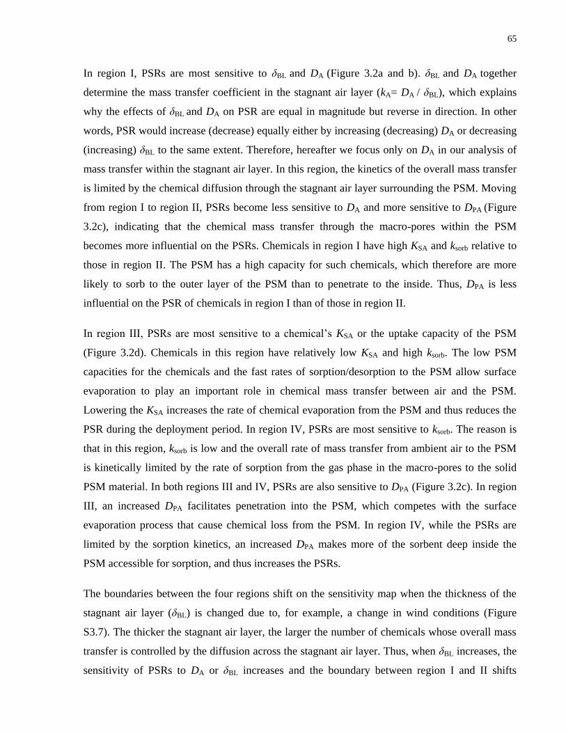
65

In region I, PSRs are most sensitive to δBL and DA (Figure 3.2a and b). δBL and DA together

determine the mass transfer coefficient in the stagnant air layer (kA= DA / δBL), which explains

why the effects of δBL and DA on PSR are equal in magnitude but reverse in direction. In other

words, PSR would increase (decrease) equally either by increasing (decreasing) DA or decreasing

(increasing) δBL to the same extent. Therefore, hereafter we focus only on DA in our analysis of

mass transfer within the stagnant air layer. In this region, the kinetics of the overall mass transfer

is limited by the chemical diffusion through the stagnant air layer surrounding the PSM. Moving

from region I to region II, PSRs become less sensitive to DA and more sensitive to DPA (Figure

3.2c), indicating that the chemical mass transfer through the macro-pores within the PSM

becomes more influential on the PSRs. Chemicals in region I have high KSA and ksorb relative to

those in region II. The PSM has a high capacity for such chemicals, which therefore are more

likely to sorb to the outer layer of the PSM than to penetrate to the inside. Thus, DPA is less

influential on the PSR of chemicals in region I than of those in region II.

In region III, PSRs are most sensitive to a chemical’s KSA or the uptake capacity of the PSM

(Figure 3.2d). Chemicals in this region have relatively low KSA and high ksorb. The low PSM

capacities for the chemicals and the fast rates of sorption/desorption to the PSM allow surface

evaporation to play an important role in chemical mass transfer between air and the PSM.

Lowering the KSA increases the rate of chemical evaporation from the PSM and thus reduces the

PSR during the deployment period. In region IV, PSRs are most sensitive to ksorb. The reason is

that in this region, ksorb is low and the overall rate of mass transfer from ambient air to the PSM

is kinetically limited by the rate of sorption from the gas phase in the macro-pores to the solid

PSM material. In both regions III and IV, PSRs are also sensitive to DPA (Figure 3.2c). In region

III, an increased DPA facilitates penetration into the PSM, which competes with the surface

evaporation process that cause chemical loss from the PSM. In region IV, while the PSRs are

limited by the sorption kinetics, an increased DPA makes more of the sorbent deep inside the

PSM accessible for sorption, and thus increases the PSRs.

The boundaries between the four regions shift on the sensitivity map when the thickness of the

stagnant air layer (δBL) is changed due to, for example, a change in wind conditions (Figure

S3.7). The thicker the stagnant air layer, the larger the number of chemicals whose overall mass

transfer is controlled by the diffusion across the stagnant air layer. Thus, when δBL increases, the

sensitivity of PSRs to DA or δBL increases and the boundary between region I and II shifts

66

towards the centre of map. As the kinetic resistance to diffusion through the stagnant air layer

increases with increasing δBL, so does the kinetic resistance to evaporation from the PSM. This

decreases the influence of surface evaporation on the PSRs for chemicals for which this process

is important (i.e., chemicals with low KSA). Therefore, region III shifts towards the lower KSA

with increased δBL. As the kinetics for chemical crossing the stagnant air layer becomes more

influential to the overall uptake, the sorption rate would have to be lower in order to kinetically

limit the overall uptake process. Thus, region IV shifts towards lower ksorb as δBL increases.

Comparing the sensitivity maps based on the models for XAD-PAS and PUF-PAS (Figure S3.7),

region I for the PUF-PAS extends to lower KSA and lower ksorb than for the XAD-PAS, indicating

that the stagnant air layer resistance (DA/δBL) is more important in determining the PSR in PUF-

PAS than in XAD-PAS. This difference could be due to differences in the configuration

(cylindrical XAD-resin filled mesh cylinder vs. planar PUF sheet) and/or physical properties

(density and macro-pore fraction) of the PSM. To investigate the contributions of these two

factors, we conducted a sensitivity analysis using models in which the cylindrical XAD-filled

mesh cylinder in the XAD-PAS model was replaced by a cylindrical PUF of the same dimension

or the PUF disk in the PUF-PAS model was changed to an XAD disk. The sensitivity maps

based on the modified models (Figure S3.8) indicate that it is the density and porosity (Table

S3.1) of the PSMs rather than their geometrical arrangement that explains the difference in the

importance of the stagnant boundary layer.

A specific chemical with known KSA and ksorb is represented by a point on the sensitivity maps.

KSAs for both XAD and PUF have been well characterized and are generally positively correlated

with molecular size. So far, information on the rates of sorption and desorption (i.e., ksorb and

kdes) to PSM is lacking. However, based on the theory of mass transfer between a fluid and a

single spherical particle,142

ksorb is positively correlated with the molecular diffusivity in the fluid

and thus negatively correlated with the molecular volume. Therefore, KSA is presumably

negatively correlated with ksorb. As such, points representing real chemicals on the sensitivity

map are more likely to distribute within a belt from the top left to the bottom right and the

likelihoods for a chemical to have both high (low) KSA and high (low) ksorb (i.e. distributed in the

upper right and lower left region of the map) are low.

67

3.4.2 Influence of Chemical Properties and Temperatures on Passive Air Sampling Rates.

Figure 3.3 Illustration of the dependence of passive sampling rates (PSRs) on chemical

properties and temperature. Molecular size: M1 > M2; temperature T1 < T2. The map depicting

PSRs in the KSA-ksorb chemical space was constructed based on the model for a XAD-passive air

sampler deployed for 360 d assuming a stagnant air boundary layer thickness δBL of 0.01 cm.

PSRs exceeding 5 m3/d were calculated for the combination of large KSA and large ksorb (hatched

area), which is unlikely to exist among real chemicals.

log KSA

log

(kSo

rb/

d–1

)

6 7 8 9 1010

4

105

106

107

108

109

ksorb(d

-1)

log KSA

0.250

1.25

2.25

3.25

4.25

5.00

6 7 8 9 1010

4

105

106

107

108

109

k sorb(d

-1)

log KSA

0.2500.5000.7501.001.251.501.752.002.252.502.753.003.253.503.754.004.254.504.755.00

0

1

5

0.5

1.52

2.5

3

3.5

44.5

PSR (m3/d)

6 7 8 9 10

9

8

7

6

5

4

T1

T2

T1

T2

M1

M2

M1

M2

68

In order to explain the variation of PSRs with temperature and between different compounds, we

constructed a chemical space map displaying the PSR calculated for different combinations of

KSA and ksorb. As an illustration, the chemical space map showing the PSR for uptake in an XAD-

PAS deployed for 360 d assuming δBL= 0.01 cm is shown in Figure 3.3. A color scale represents

the PSR with changes in KSA and ksorb. Maps with lower and higher wind exposure of the XAD-

PAS (δBL= 0.1 and 0.001cm) are presented in Figure S3.9. Recall that KSA is correlated with DA

and DPA (Figure S3.5) and thus the maps integrate the variation of DA and DPA with KSA. The

maps display L-shaped strips of different colors, each representing a range of PSRs. The dashed

line connecting the inflection points of all the L-shaped strips divides the map into two regions.

On the upper-left (lower-right) region, the strips are generally parallel with the y-axis (x-axis),

indicating PSRs for chemicals in this region are sensitive to changes in KSA (ksorb) but not

sensitive to the changes in ksorb (KSA). This pattern of PSRs in the chemical space map agrees

with the results of the sensitivity analysis (Figure 3.2d and e).

The hatched area on the top right of the map represents a PSR above 5 m3/d, which has rarely

been observed in a field calibration using the XAD-PAS. As mentioned before, KSA is generally

negatively correlated with ksorb; smaller chemicals in a homologous series tend to have a low KSA

and a high ksorb. Therefore, points representing a homologous series on the map would distribute

along a line from the bottom right to the top left and a point representing a chemical on the

chemical space map would shift towards the upper left (lower right) at higher (lower)

temperatures. As indicated by the model results, different chemicals or a chemical at different

temperatures would be expected to have different PSRs. Depending on the chemical properties

(KSA and ksorb), the direction in which the PSR changes with chemical properties and

temperatures can be different. For chemicals in the lower right of the map (high KSA and low

ksorb), the PSR for a homologous series decreases with increasing molecular size (M1 > M2 in

Figure 3.3). In contrast, if the sorption of the chemicals to the sorbent is fast (ksorb is large) so that

the chemicals are positioned on the upper left, a chemical with large molecular size (M1) would

have a higher PSR than a smaller chemical (M2). Similarly, the variation of the PSR with

temperature can be different depending on a chemical’s KSA and ksorb, i.e. its position in the map.

PSRs for chemicals positioned in the lower right (upper left) increase (decrease) as temperature

increases (from T1 to T2 as illustrated in Figure 3.3).

69

The model facilitates a mechanistic explanation of this seemingly contradictory behavior. The

PSR of chemicals in the lower right is kinetically controlled by the sorption process and the

diffusion within the PSM. As KSA decreases and ksorb increases with a decrease in molecular size

or an increase in temperature, the fraction in the air-filled pores increases, facilitating the

penetration into the PSM. The increased diffusivity within the PSM and the increased sorption

rate (ksorb) will increase the PSR. For chemicals in the upper left region, ksorb is large so that

chemicals accumulate rapidly at the PSM surface. Increased chemical accumulation at the

surface with increased ksorb and the decreased sorbent capacity (KSA) would enhance the role that

surface evaporation plays in decreasing the PSR.

Many studies on passive air sampling have observed the variation of PSRs among different

chemicals or for a chemical at different temperatures.20,87,89,90

For the XAD-PAS, PSRs were

found to be positively correlated with DA but the variation in PSR was much larger than that of

DA.20,89

For the PUF-PAS, the relationship between PSRs and DA seems more complicated. Some

studies observed a negative correlation of PSRs with DA: higher PSRs for chemicals at lower

temperatures and for highly chlorinated biphenyls.87,90

On the contrary, lower PSRs for highly

brominated diphenyl ethers have also been observed.104

One explanation for the variation of

PSRs in PUF-PAS is a shift in the gas-particle distribution of the target SVOCs:87

at lower

(higher) temperature or for a heavier (lighter) congener, a higher (lower) fraction of the

chemicals would be in the particle phase so the amount of chemicals in the gas phase available

for uptake decreases (increases). Considering a lower sampling efficiency for particle-bound

chemicals than for chemicals in the gas phase, PSR calibrated against bulk air concentrations

becomes lower (higher). Although this process could possibly affect the PSR of SVOCs with

very low volatility (e.g. highly brominated diphenyl ethers), it cannot explain the PSR variation

for chemicals predominantly in gas phase (e.g. tri- and tetra-chlorinated biphenyls). Comparing

the field observations with the map in Figure 3.3, it seems that a model that considers the kinetic

resistance within the PSM can explain the observed PSR variations for both XAD-PAS and PUF-

PAS. The observed behavior of the XAD-PAS agrees with the case on the bottom right of the

map (higher KSA and lower ksorb) and that of the PUF-PAS follows that in the upper left region

(lower KSA and higher ksorb). While KSA for XAD has been found to be generally higher than that

for PUF, no information on ksorb for XAD or PUF is currently available. Because sorption to

70

XAD involves diffusion through the meso-pores within each pellet, which may limit the sorption

kinetics, ksorb for XAD is presumably lower than for PUF.

3.4.3 Two-Stage Uptake Process.

In the PUF-PAS calibration studies by Chaemfa et al.88

and by Tsurukawa et al.,128

some

chemicals are observed to have a high PSR initially (~1-2 weeks) after which the PSR drops and

stays relatively constant. A two-stage uptake was hypothesized to explain such an observation

but no quantitative studies were conducted and no mechanistic explanation was formulated. We

used the model to construct the uptake curves for chemicals with different combinations of KSA

and ksorb (Figure S3.10). Two-stage uptake was predicted for chemicals with high ksorb. Sorption

of such chemicals to the surface of the PSM is faster than diffusive penetration into the PSM.

Initially, sorption occurs at the surface of the PSM, the resistance to diffusion in the PSM pores

is not rate-controlling, and the PSR is determined by the fast sorption rate. As the PSM surface

becomes saturated, the chemical either evaporates or diffuses into the PSM. The overall uptake

kinetics is then determined by the rate of diffusion into the PSM, which leads to a decreased PSR

compared with the initial uptake phase. Although the model can mechanistically explain a two-

stage uptake, we are unable to use the model to predict the uptake for specific compounds due to

the of lack information on ksorb.

3.4.4 Non-Uniform Chemical Distribution within Passive Sampling Media.

The model describing the mass transfer processes within PSMs is capable of calculating the

radial distribution of chemicals within the PSM. Agreeing with experimental evidence,(Chapter

2)126

the model calculations for the KSA-ksorb chemical space indicate a non-uniform chemical

distribution within the PSMs. For the majority of KSA and ksorb combinations, >90% of the

amount of chemical accumulated in the PSM of both XAD- and PUF-PAS are constrained within

a surface layer of less than 0.4 cm thickness after 90 d of deployment (Figure S3.11). Our

experiments investigating chemical distribution within the PSMs were based on cylindrical PSM

configurations (Chapter 2)126

. The mass transfer of chemicals within such cylindrical PSMs

might be retarded as the cross-sectional area for diffusion decreases from the outer to the inner

part of the PSM. This could possibly add some uncertainty when extrapolating the experimental

results based on PSMs of cylindrical configuration to those of planar configuration (disk). Model

71

calculations for PSMs in both cylindrical and planar configurations (Figure S3.11) revealed no

obvious differences in the penetration depth (defined as the thickness of the outer PSM layer

which accumulates 90% of the sampled amount). This indicates that the non-uniform distribution

within the PSM is mainly determined by the competition between sorption and diffusion deeper

into the PSM rather than the PSM configuration.

3.4.5 Knowledge Gap and Implications.

In this study, the new model was primarily used to provide mechanism insight into some field

observations that could not be explained with the two-film PAS theory. The new model’s

capability to describe the behavior of specific chemicals is mainly limited by the lack of

quantitative information on ksorb, either from measurements or predictions. Unlike other model

parameters such as DA, DPA and KSA, which either have been measured or can be predicted with

established theories for SVOCs,38,109,119

ksorb has only been studied for the sorption of some

VOCs (e.g. benzene, carbon tetrachloride) on a few sorbents other than XAD or PUF.136,143

In

order to quantitatively describe specific chemicals and to expand the application of the model,

ksorb and its temperature dependence need to be quantified for SVOCs and the PSMs commonly

used in PASs. Once ksorb is available for specific chemicals, this model could be used to predict

chemical specific PSRs at different temperatures. The model results on the chemical distribution

within the PSMs could also be useful when optimizing the design of PASs with the intention of

improving the sampling efficiency. For example, increasing the interfacial area/volume ratio of a

PSM would prevent the sorbent in the inner part of the PSM from being wasted.

In field applications of PASs, PSRs are often determined from calibrations against active air

samplers instead of being calculated from PAS theory. Therefore, although both experimental

(Chapter 2) 126

and modeling evidence (this study) indicates non-uniform chemical distribution

within porous PSMs, which contradicts the assumption in the two-film approach, interpretation

of PAS data using empirically derived PSRs will not be affected, as long as PSRs are used that

are compound- and sampling site specific. The two-film PAS theory has previously been used to

estimate linear uptake ranges9,38,87

or to calculate PSRs from the observed loss of depuration

compounds.95

By neglecting to consider the kinetic resistance within the PSM, linear uptake

ranges tend to be overestimated because deeper parts of the PSM are not readily accessible. This

agrees with observed linear uptake ranges that are shorter than estimated for heavier compounds

72

that do not penetrate readily into the PSMs.95

PSRs, through their dependence on KSA and ksorb,

are clearly compound-specific, and the applicability of a PSR obtained for one type of

(depuration) compound to another cannot be assumed but would need to be demonstrated. Even

if depuration compounds are isotopically labeled analogs of the target compounds, PSRs derived

from the loss of depuration compounds (without accounting for a kinetic resistance within the

PSM) may deviate from the PSRs of chemicals sampled from air because their distributions

within the PSM are different and thus result in different kinetic resistances within the PSM.

3.5 Acknowledgments

We acknowledge research funding from the Canadian Foundation for Climate and Atmospheric

Sciences and the Natural Sciences and Engineering Research Council of Canada. X. Zhang

acknowledges financial support from an Ontario Graduate Scholarship.

73


Mathematical Model of Chemical Uptake by XAD-PAS.

Discretization of Partial Differential Equations. As illustrated in Figure S3.1, the governing

partial differential equations (Equation 3.1, 3.3, 3.6) of the model can be discretized on the

spatial derivative with finite differences into a system of ordinary differential equations:

1 1 1 1

A A A A A A

A A2

A S A A

2 1, 1 1

( ) 2

i i i i i idC C C C C C

D D m i m ndt r i m

(Equation S3.1)

1 1 1 1

sorbA A A A A A

PA PA A des S2

S S S

2 1, 1 1

2

i i i i i i

i ikdC C C C C CD D C k C i m

dt i(Equation S3.2)

S sorb

A des S , 1 1

i

i idC kC k C i m

dt (Equation S3.3)

The system of ordinary differential equations can be solved with information on initial

conditions and boundary/interfacial conditions.

Initial Conditions. Initially (t = 0), the chemical concentration in the air surrounding the PSM

(XAD mesh cylinder) equals the ambient air concentration (CAA, ng/cm3):

A AA S S( , 0) ,

BLC r C r r r (Equation S3.4)

or A AA

(0) , 1 i

C C m i m n (Equation S3.4’)

Chemicals initially in the PSM (e.g. deliberately spiked depuration compounds) are assumed to

be uniformly distributed within the PSM and to have reached equilibrium between PSM and

macroporous air:

0

A S

S SA

( , 0) , 0(1 - )

nC r r r

V K (Equation S3.5)

or 0

A

S SA

(0) , 0(1 - )

i nC i m

V K (Equation S3.5’)

74

0 SA

S S

S SA

(1 - )( , 0) , 0

(1 - )

n KC r r r

V K (Equation S3.6)

or 0 SA

S

S SA

(1 - )(0) , 0

(1 - )

i n KC i m

V K (Equation S3.6)

where VS (cm3) is the volume of the PSM. For depuration compounds spiked to the PSM at the

beginning of a passive air sampling campaign, n0 (ng) is the initial amount within the PSM. For

the target chemicals sampled by the PAS, n0 equals the blank level of the chemicals in the PSM.

Assuming blank levels are negligible, Equation S3.5and Equation S3.6 become:

A S S( , 0) ( , 0) 0 , 0 C r C r r r (Equation S3.7)

or A S

(0) (0) 0 , 0 i i

C C i m (Equation S3.7’)

Boundary/Interfacial Conditions. At the cylindrical axis of the XAD mesh cylinder (r = 0 or i =

0), because of symmetry, there is no radial flux, therefore:

A(0, )

0 ,

C tt

r (Equation S3.8)

From Equation 3.3 and Equation S3.6,

SA(0, )(0, )

C tC t

t t (Equation S3.9)

or 00

0 0SA

sorb A des S

dCdCk C k C

dt dt (Equation S3.9’)

At the interface between the PSM and stagnant air (r = rS or i = m), applying a mass balance

equation to the macroporous air phase of an imaginary layer between rS – 0.5δS and rS + 0.5δA,

we obtain:

1 1

A A A A A

A PA sorb A des S

A A

( )2

m m m m m

m mS A

S

dC C C C CD D k C k C

dt (Equation S3.10)

75

S sorb

A des S

m

m mdC kC k C

dt (Equation S3.11)

At the boundary of the stagnant air layer (r = rS + δBL or i = m + n), applying a mass balance

equation to an imaginary layer between rS + δBL – 0.5δA and rS + δBL + 0.5δA, we get:

1

A AA A A

A 2

A

2

m n m n m ndC C C C

Ddt

(Equation S3.12)

An ordinary differential equation system (A

iC and

S

jC as dependents of t, where i = 0…m + n; j =

0…m) composed by Equation S3.1 to Equation S3.8 can be solved numerically to get A

iC and

S

jC at a given time t.

Figure S3.1 Illustration showing the discretization of the PSM of the XAD-PAS to solve the

diffusion equations. m = 200 and n = 50 were used in this study.

01

i=-1

m-1

m+1m

2

m+n-1m+n

rS

δBL

2 cm

10

cm

76

Mathematical Model of Chemical Uptake by PUF-PAS.

Diffusion and Sorption/Desorption Equations. Different from the XAD-PAS, whose PSM is

cylindrical, the widely used PUF-PAS has a PUF disk as the PSM. Chemical mass transfer

within the PUF disk can be modeled using the diffusion equations for a planar sheet. The

equations corresponding to Equation 3.1, 3.3, 3.6 are:

2

A A

A BL2

( , ),

C z t CD L z L

t z (Equation S3.13)

2

SA A

PA 2

( , ), 0

CC z t CD z L

t z t (Equation S3.14)

S A

S

( , ), 0

sorb

des

C z t k Ck C z L

t (Equation S3.15)

where L (cm) is half of the thickness of the PUF disk; z (cm) is the position at the coordinate

originated from the half thickness of the PUF disk (Figure S3.2).

Equation S3.13, Equation S3.14, and Equation S3.15 can be discretized as:

1 1

A A A A

A 2

A

2, 1 1

i i i idC C C C

D m i m ndt

(Equation S3.16)

1 1

sorbA A A A

PA A des S2

S

2, 1 1

i i i i

i ikdC C C CD C k C i m

dt (Equation S3.17)

S sorb

A des S , 1 1

i

i idC kC k C i m

dt (Equation S3.18)

Initial Conditions. Initially (t = 0), chemical concentration in the air surrounding the PUF disk

equals the ambient air concentration (CAA, ng/cm3):

A AA( , 0) ,

BLC z C L z L (Equation S3.19)

or A AA

(0) , 1 i

C C m i m n (Equation S3.19’)

77

Chemicals initially in the PUF are assumed uniformly distributed and reach equilibrium between

PUF and macroporous air:

0

A

S SA

( , 0) , 0(1 - )

nC z z L

V K (Equation S3.20)

or 0

A

S SA

(0) , 0(1 - )

i nC i m


0 SA

S

S SA

(1 - )( , 0) , 0

(1 - )

n KC z z L

V K (Equation S3.21)

0 SA

S

S SA

(1 - )(0) , 0

(1 - )

i n KC i m


where VS (cm3) is the volume of the PUF disk; For depuration compounds spiked to the PUF at

the beginning of passive air sampling campaign, n0 (ng) is the amount of depuration compounds

within the PUF initially. For the target chemicals sampled by the PAS, n0 equals the blank level

of the chemicals on the PUF. Assuming blank levels are negligible, Equation S3.20 and Equation

S3.21 become:

A S S( , 0) ( , 0) 0 , 0 C r C r r r (Equation S3.22)

or A S

(0) (0) 0 , 0 i i

C C i m (Equation S3.22’)

Boundary/Interfacial Conditions. At the half depth of the PUF disk (z = 0 or i = 0), because of

symmetry, there is no radial flux, therefore:

A(0, )

0 ,

C tt

z (Equation S3.23)

From Equation S3.14 and Equation S3.23,

SA(0, )(0, )

C tC t

t t (Equation S3.24)

or 00

0 0SA

sorb A des S

dCdCk C k C

dt dt (Equation S3.24’)

78

At the interface between the PUF and stagnant air (z = L or i = m), applying a mass balance

equation to the macroporous air phase of an imaginary layers between L – 0.5δS and L + 0.5δA,

we have:

1 1

A A A A A

A PA sorb A des S

A A

( )2

m m m m m

m mS A

S

dC C C C CD D k C k C

dt (Equation S3.25)

S sorb

A des S

m

m mdC kC k C

dt (Equation S3.26)

At the boundary of the stagnant air layer (z = L + δBL or i = m + n), applying a mass balance

equation to an imaginary layers between L + δBL – 0.5δA and L + δBL + 0.5δA, we get:

1

A AA A A

A 2

A

2

m n m n m ndC C C C

Ddt

(Equation S3.27)

An ordinary differential equation system (A

iC and

S

jC as dependents of t, where i = 0…m + n; j =

0…m) composed by Equation S3.16, Equation S3.17, Equation S3.18, Equation S3.22, Equation

S3.20, Equation S3.21, Equation S3.24, Equation S3.25, Equation S3.26, and Equation S3.27 can

be solved numerically to get A

iC and

S

jC at a given time t.

79

Figure S3.2 Illustration showing the discretization of the PSM of the PUF-PAS to solve the

diffusion equations. m = 200 and n = 50 were used in this study.

14 cm

1.5 cm

L

L

i=0…

…

i=1

i=-1

i=m-1

i=m+1i=m

zi

…

i=m+n-1i=m+n

δS = rS /m

δA = δBL /n

80

Table S3.1 Properties of the modeled passive air sampling media

PAS

PSM Radius

(cm)

PSM

Height/Thickness

(cm)

Density

(g/cm3)

Void

fraction, ε

1 10 1.08 ref.130

0.45 ref.130

14 1.5 0.0213 ref.9

0.97 ref.119

81

Figure S3.3 Illustration of how passive air sampling rates (PSRs) were derived from a linear

fit on six discrete data points placed equidistantly on the uptake curve generated by the model.

Figure S3.4 Distribution of the difference between KXAD/A and KPUF/A for chlorothalonil,

endosulfan I, endosulfan II, atrazine, alachlor, metolachlor, trifluralin, HCB, α-HCH, γ-HCH and

209 PCB congeners based on calculations using polyparameter linear free energy relationships

(ppLFERs).38,111,119

0 10 20 30 40 50 60 70 80 90

0

20

40

60

80

100

120

140

160

180

200

PAS deployment time (d)

Equiv

ale

nt

sa

mplin

g vo

lum

e (

m3) Fit line based on the data points

PAS sampling rate = slope =2.3 m3/d

-0.4 0.0 0.4 0.8 1.2 1.6 2.0 2.40

10

20

30

40

50

Num

be

r o

f o

bse

rva

tio

n

μ=0.800, σ=0.386

log KXAD/A - log KPUF/A

82

Figure S3.5 Empirical relationships of XAD/air partition coefficient (KXAD/A) and PUF/air

partition coefficient (KPUF/A)with the diffusivity of chemicals in air (DA, cm2/s) based on 209

polychlorinated biphenyl congeners and 10 organochlorinated pesticides (namely, chlorothalonil,

endosulfan I, endosulfan II, atrazine, alachlor, metolachlor, trifluralin, HCB, α-HCH, and γ-

HCH). KXAD/A and KPUF/A of the chemicals were calculated using polyparameter linear free

energy relationships (ppLFERs).38,111,119

DA was calculated using the Fuller-Schettler-Giddings

equation with La Bas molar volumes.109

7.0 8.0 9.0 10.0 11.00.030

0.035

0.040

0.045

0.050

0.055

log KXAD/A

DA

/ (

cm2 s

-1)

DA /(cm2s-1)= -0.0041logKXAD/A+0.0781

R2 = 0.821

T = 281K

6.0 7.0 8.0 9.0 10.0

0.038

0.042

0.046

0.050

0.054

0.058DA /(cm2s-1)= -0.0044logKXAD/A+0.0822

R2 = 0.825

T = 293K

5 6 7 8 9 10 11 120.034

0.038

0.042

0.046

0.050

0.054

4 5 6 7 8 9 10 11

0.038

0.042

0.046

0.050

0.054

0.058

T = 281K T = 293K

DA /(cm2s-1)= -0.0024logKPUF/A+0.0623

R2 = 0.762

DA /(cm2s-1)= -0.0028logKPUF/A+0.0667

R2 = 0.763

log KPUF/A

83

Figure S3.6 Illustration of the relationship between the change of internal energy (ΔUSA,

from air phase M to sorbed phase M···S) and the activation energies of sorption (Ea+) and

desorption (Ea–).

M

M···S

Ea+

Ea–

ΔUSAPo

ten

tial

En

ergy

84

Figure S3.7 Sensitivities of passive air sampling rate (m3/d) of XAD-PAS (left) and PUF-

PAS (right) (deployed for 90 d) to changes of molecular diffusivity in bulk air (DA), molecular

diffusivity in the macroporous fraction within the PSM (DPA), equilibrium partition coefficient

between the sorbent and air (KSA), and the sorption rate constant (ksorb) based on stagnant

boundary layer thickness δBL of 0.001 cm (top), 0.01 cm (centre), and 0.1 cm (bottom).

δB

L=

0.0

1 c

mδ

BL

= 0

.00

1 c

mδ

BL

= 0

.1 c

m

6 7 8 9 10

10000

100000

1000000

1E7

1E8

1E9

D

B

-1.000-0.9000-0.8000-0.7000-0.6000-0.5000-0.4000-0.3000-0.2000-0.10000.0000.10000.20000.30000.40000.50000.60000.70000.80000.90001.000

6 7 8 9 10

10000

100000

1000000

1E7

1E8

1E9

D

B

-1.000-0.9000-0.8000-0.7000-0.6000-0.5000-0.4000-0.3000-0.2000-0.10000.0000.10000.20000.30000.40000.50000.60000.70000.80000.90001.000

6 7 8 9 10

10000

100000

1000000

1E7

1E8

1E9

D

B

-1.000-0.9000-0.8000-0.7000-0.6000-0.5000-0.4000-0.3000-0.2000-0.10000.0000.10000.20000.30000.40000.50000.60000.70000.80000.90001.000

6 7 8 9 10

10000

100000

1000000

1E7

1E8

1E9

D

B

-1.000-0.9000-0.8000-0.7000-0.6000-0.5000-0.4000-0.3000-0.2000-0.10000.0000.10000.20000.30000.40000.50000.60000.70000.80000.90001.000

6 7 8 9 10

log KXAD/A

9

8

7

6

5

4

log

(kSo

rb/

d–1

)

9

8

7

6

5

4

9

8

7

6

5

4

6 7 8 9 10

6 7 8 9 10 6 7 8 9 10

5 6 7 8 9

10000

100000

1000000

1E7

1E8

1E9

D

B

-1.000-0.9000-0.8000-0.7000-0.6000-0.5000-0.4000-0.3000-0.2000-0.10000.0000.10000.20000.30000.40000.50000.60000.70000.80000.90001.000

0

0.2

1.0

0.4

0.6

0.8

-1.0

-0.8

-0.6

-0.4

-0.2

6 7 8 9 10

10000

100000

1000000

1E7

1E8

1E9

D

B

-1.000-0.9000-0.8000-0.7000-0.6000-0.5000-0.4000-0.3000-0.2000-0.10000.0000.10000.20000.30000.40000.50000.60000.70000.80000.90001.000

6 7 8 9 10

10000

100000

1000000

1E7

1E8

1E9

D

B

-1.000-0.9000-0.8000-0.7000-0.6000-0.5000-0.4000-0.3000-0.2000-0.10000.0000.10000.20000.30000.40000.50000.60000.70000.80000.90001.000

6 7 8 9 10

10000

100000

1000000

1E7

1E8

1E9

D

B

-1.000-0.9000-0.8000-0.7000-0.6000-0.5000-0.4000-0.3000-0.2000-0.10000.0000.10000.20000.30000.40000.50000.60000.70000.80000.90001.000

6 7 8 9 10

10000

100000

1000000

1E7

1E8

1E9

D

B

-1.000-0.9000-0.8000-0.7000-0.6000-0.5000-0.4000-0.3000-0.2000-0.10000.0000.10000.20000.30000.40000.50000.60000.70000.80000.90001.000

6 7 8 9 10

log KXAD/A

9

8

7

6

5

4

log

(kSo

rb/

d–1

)

9

8

7

6

5

4

9

8

7

6

5

4

6 7 8 9 10

6 7 8 9 10 6 7 8 9 10

5 6 7 8 9

10000

100000

1000000

1E7

1E8

1E9

D

B

-1.000-0.9000-0.8000-0.7000-0.6000-0.5000-0.4000-0.3000-0.2000-0.10000.0000.10000.20000.30000.40000.50000.60000.70000.80000.90001.000

0

0.2

1.0

0.4

0.6

0.8

-1.0

-0.8

-0.6

-0.4

-0.2

6 7 8 9 10

10000

100000

1000000

1E7

1E8

1E9

D

B

-1.000-0.9000-0.8000-0.7000-0.6000-0.5000-0.4000-0.3000-0.2000-0.10000.0000.10000.20000.30000.40000.50000.60000.70000.80000.90001.000

6 7 8 9 10

10000

100000

1000000

1E7

1E8

1E9

D

B

-1.000-0.9000-0.8000-0.7000-0.6000-0.5000-0.4000-0.3000-0.2000-0.10000.0000.10000.20000.30000.40000.50000.60000.70000.80000.90001.000

6 7 8 9 10

10000

100000

1000000

1E7

1E8

1E9

D

B

-1.000-0.9000-0.8000-0.7000-0.6000-0.5000-0.4000-0.3000-0.2000-0.10000.0000.10000.20000.30000.40000.50000.60000.70000.80000.90001.000

6 7 8 9 10

10000

100000

1000000

1E7

1E8

1E9

D

B

-1.000-0.9000-0.8000-0.7000-0.6000-0.5000-0.4000-0.3000-0.2000-0.10000.0000.10000.20000.30000.40000.50000.60000.70000.80000.90001.000

6 7 8 9 10

log KXAD/A

9

8

7

6

5

4

log

(kSo

rb/

d–1

)

9

8

7

6

5

4

9

8

7

6

5

4

6 7 8 9 10

6 7 8 9 10 6 7 8 9 10

5 6 7 8 9

10000

100000

1000000

1E7

1E8

1E9

D

B

-1.000-0.9000-0.8000-0.7000-0.6000-0.5000-0.4000-0.3000-0.2000-0.10000.0000.10000.20000.30000.40000.50000.60000.70000.80000.90001.000

0

0.2

1.0

0.4

0.6

0.8

-1.0

-0.8

-0.6

-0.4

-0.2

XAD-PAS PUF-PAS

9

8

7

6

5

4

9

8

7

6

5

4

9

8

7

6

5

4

9

8

7

6

5

4

9

8

7

6

5

4

9

8

7

6

5

4

5 6 7 8 9

10000

100000

1000000

1E7

1E8

1E9

D

B

-1.000-0.9000-0.8000-0.7000-0.6000-0.5000-0.4000-0.3000-0.2000-0.10000.0000.10000.20000.30000.40000.50000.60000.70000.80000.90001.000

5 6 7 8 9

10000

100000

1000000

1E7

1E8

1E9

D

B

-1.000-0.9000-0.8000-0.7000-0.6000-0.5000-0.4000-0.3000-0.2000-0.10000.0000.10000.20000.30000.40000.50000.60000.70000.80000.90001.000

5 6 7 8 9

10000

100000

1000000

1E7

1E8

1E9

D

B

-1.000-0.9000-0.8000-0.7000-0.6000-0.5000-0.4000-0.3000-0.2000-0.10000.0000.10000.20000.30000.40000.50000.60000.70000.80000.90001.000

5 6 7 8 9

10000

100000

1000000

1E7

1E8

1E9

D

B

-1.000-0.9000-0.8000-0.7000-0.6000-0.5000-0.4000-0.3000-0.2000-0.10000.0000.10000.20000.30000.40000.50000.60000.70000.80000.90001.000

5 6 7 8 9

10000

100000

1000000

1E7

1E8

1E9

D

B

-1.000-0.9000-0.8000-0.7000-0.6000-0.5000-0.4000-0.3000-0.2000-0.10000.0000.10000.20000.30000.40000.50000.60000.70000.80000.90001.000

5 6 7 8 9

9

8

7

6

5

4

9

8

7

6

5

4

9

8

7

6

5

4

5 6 7 8 9

5 6 7 8 9 5 6 7 8 9

5 6 7 8 9

10000

100000

1000000

1E7

1E8

1E9

D

B

-1.000-0.9000-0.8000-0.7000-0.6000-0.5000-0.4000-0.3000-0.2000-0.10000.0000.10000.20000.30000.40000.50000.60000.70000.80000.90001.000

0

0.2

1.0

0.4

0.6

0.8

-1.0

-0.8

-0.6

-0.4

-0.2

log

(kSo

rb/

d–1

)5 6 7 8 9

10000

100000

1000000

1E7

1E8

1E9

DB

-1.000-0.9000-0.8000-0.7000-0.6000-0.5000-0.4000-0.3000-0.2000-0.10000.0000.10000.20000.30000.40000.50000.60000.70000.80000.90001.000

5 6 7 8 9

10000

100000

1000000

1E7

1E8

1E9

D

B

-1.000-0.9000-0.8000-0.7000-0.6000-0.5000-0.4000-0.3000-0.2000-0.10000.0000.10000.20000.30000.40000.50000.60000.70000.80000.90001.000

5 6 7 8 9

10000

100000

1000000

1E7

1E8

1E9D

B

-1.000-0.9000-0.8000-0.7000-0.6000-0.5000-0.4000-0.3000-0.2000-0.10000.0000.10000.20000.30000.40000.50000.60000.70000.80000.90001.000

5 6 7 8 9

9

8

7

6

5

4

9

8

7

6

5

4

9

8

7

6

5

4

5 6 7 8 9

5 6 7 8 9 5 6 7 8 9

5 6 7 8 9

10000

100000

1000000

1E7

1E8

1E9

D

B

-1.000-0.9000-0.8000-0.7000-0.6000-0.5000-0.4000-0.3000-0.2000-0.10000.0000.10000.20000.30000.40000.50000.60000.70000.80000.90001.000

0

0.2

1.0

0.4

0.6

0.8

-1.0

-0.8

-0.6

-0.4

-0.2

log KPUF/A

5 6 7 8 9

10000

100000

1000000

1E7

1E8

1E9

D

B

-1.000-0.9000-0.8000-0.7000-0.6000-0.5000-0.4000-0.3000-0.2000-0.10000.0000.10000.20000.30000.40000.50000.60000.70000.80000.90001.000

5 6 7 8 9

10000

100000

1000000

1E7

1E8

1E9

D

B

-1.000-0.9000-0.8000-0.7000-0.6000-0.5000-0.4000-0.3000-0.2000-0.10000.0000.10000.20000.30000.40000.50000.60000.70000.80000.90001.000

5 6 7 8 9

10000

100000

1000000

1E7

1E8

1E9

D

B

-1.000-0.9000-0.8000-0.7000-0.6000-0.5000-0.4000-0.3000-0.2000-0.10000.0000.10000.20000.30000.40000.50000.60000.70000.80000.90001.000

5 6 7 8 9

10000

100000

1000000

1E7

1E8

1E9

D

B

-1.000-0.9000-0.8000-0.7000-0.6000-0.5000-0.4000-0.3000-0.2000-0.10000.0000.10000.20000.30000.40000.50000.60000.70000.80000.90001.000

5 6 7 8 9

9

8

7

6

5

4

9

8

7

6

5

4

9

8

7

6

5

4

5 6 7 8 9

5 6 7 8 9 5 6 7 8 9

5 6 7 8 9

10000

100000

1000000

1E7

1E8

1E9

D

B

-1.000-0.9000-0.8000-0.7000-0.6000-0.5000-0.4000-0.3000-0.2000-0.10000.0000.10000.20000.30000.40000.50000.60000.70000.80000.90001.000

0

0.2

1.0

0.4

0.6

0.8

-1.0

-0.8

-0.6

-0.4

-0.2

log KPUF/A

log KPUF/A

log

(kSo

rb/

d–1

)lo

g (k

Sorb

/ d–1

)

85

Figure S3.8 Comparison between cylindrical and disk-like PSM configurations for the

sensitivities of passive air sampling rate (m3/d) to the changes of in bulk air (DA), molecular

diffusivity in the macroporous fraction within the media PSM (DPA), equilibrium partition

coefficient between the sorbent and air (KSA), and the sorption rate constant (ksorb) at a stagnant

boundary layer thickness δBL of 0.01cm.

6 7 8 9 10

10000

100000

1000000

1E7

1E8

1E9

D

B

-1.000-0.9000-0.8000-0.7000-0.6000-0.5000-0.4000-0.3000-0.2000-0.10000.0000.10000.20000.30000.40000.50000.60000.70000.80000.90001.000

6 7 8 9 10

10000

100000

1000000

1E7

1E8

1E9

D

B

-1.000-0.9000-0.8000-0.7000-0.6000-0.5000-0.4000-0.3000-0.2000-0.10000.0000.10000.20000.30000.40000.50000.60000.70000.80000.90001.000

6 7 8 9 10

10000

100000

1000000

1E7

1E8

1E9

D

B

-1.000-0.9000-0.8000-0.7000-0.6000-0.5000-0.4000-0.3000-0.2000-0.10000.0000.10000.20000.30000.40000.50000.60000.70000.80000.90001.000

6 7 8 9 10

10000

100000

1000000

1E7

1E8

1E9

D

B

-1.000-0.9000-0.8000-0.7000-0.6000-0.5000-0.4000-0.3000-0.2000-0.10000.0000.10000.20000.30000.40000.50000.60000.70000.80000.90001.000

5 6 7 8 9

10000

100000

1000000

1E7

1E8

1E9

D

B

-1.000-0.9000-0.8000-0.7000-0.6000-0.5000-0.4000-0.3000-0.2000-0.10000.0000.10000.20000.30000.40000.50000.60000.70000.80000.90001.000

5 6 7 8 9

10000

100000

1000000

1E7

1E8

1E9

D

B

-1.000-0.9000-0.8000-0.7000-0.6000-0.5000-0.4000-0.3000-0.2000-0.10000.0000.10000.20000.30000.40000.50000.60000.70000.80000.90001.000

5 6 7 8 9

10000

100000

1000000

1E7

1E8

1E9

D

B

-1.000-0.9000-0.8000-0.7000-0.6000-0.5000-0.4000-0.3000-0.2000-0.10000.0000.10000.20000.30000.40000.50000.60000.70000.80000.90001.000

5 6 7 8 9

10000

100000

1000000

1E7

1E8

1E9

D

B

-1.000-0.9000-0.8000-0.7000-0.6000-0.5000-0.4000-0.3000-0.2000-0.10000.0000.10000.20000.30000.40000.50000.60000.70000.80000.90001.000

δBL = 0.01 cm

6 7 8 9 10

10000

100000

1000000

1E7

1E8

1E9

D

B

-1.000-0.9000-0.8000-0.7000-0.6000-0.5000-0.4000-0.3000-0.2000-0.10000.0000.10000.20000.30000.40000.50000.60000.70000.80000.90001.000

6 7 8 9 10

10000

100000

1000000

1E7

1E8

1E9

D

B

-1.000-0.9000-0.8000-0.7000-0.6000-0.5000-0.4000-0.3000-0.2000-0.10000.0000.10000.20000.30000.40000.50000.60000.70000.80000.90001.000

6 7 8 9 10

10000

100000

1000000

1E7

1E8

1E9

D

B

-1.000-0.9000-0.8000-0.7000-0.6000-0.5000-0.4000-0.3000-0.2000-0.10000.0000.10000.20000.30000.40000.50000.60000.70000.80000.90001.000

6 7 8 9 10

10000

100000

1000000

1E7

1E8

1E9

D

B

-1.000-0.9000-0.8000-0.7000-0.6000-0.5000-0.4000-0.3000-0.2000-0.10000.0000.10000.20000.30000.40000.50000.60000.70000.80000.90001.000

6 7 8 9 10

log KXAD/A

9

8

7

6

5

4

log

(kSo

rb/

d–1

)

9

8

7

6

5

4

9

8

7

6

5

4

6 7 8 9 10

6 7 8 9 10 6 7 8 9 10

5 6 7 8 9

10000

100000

1000000

1E7

1E8

1E9

D

B

-1.000-0.9000-0.8000-0.7000-0.6000-0.5000-0.4000-0.3000-0.2000-0.10000.0000.10000.20000.30000.40000.50000.60000.70000.80000.90001.000

0

0.2

1.0

0.4

0.6

0.8

-1.0

-0.8

-0.6

-0.4

-0.2

5 6 7 8 9

10000

100000

1000000

1E7

1E8

1E9

D

B

-1.000-0.9000-0.8000-0.7000-0.6000-0.5000-0.4000-0.3000-0.2000-0.10000.0000.10000.20000.30000.40000.50000.60000.70000.80000.90001.000

log

(kSo

rb/

d–1

)

5 6 7 8 9

10000

100000

1000000

1E7

1E8

1E9

D

B

-1.000-0.9000-0.8000-0.7000-0.6000-0.5000-0.4000-0.3000-0.2000-0.10000.0000.10000.20000.30000.40000.50000.60000.70000.80000.90001.000

5 6 7 8 9

10000

100000

1000000

1E7

1E8

1E9

D

B

-1.000-0.9000-0.8000-0.7000-0.6000-0.5000-0.4000-0.3000-0.2000-0.10000.0000.10000.20000.30000.40000.50000.60000.70000.80000.90001.000

5 6 7 8 9

10000

100000

1000000

1E7

1E8

1E9

D

B

-1.000-0.9000-0.8000-0.7000-0.6000-0.5000-0.4000-0.3000-0.2000-0.10000.0000.10000.20000.30000.40000.50000.60000.70000.80000.90001.000

5 6 7 8 9

9

8

7

6

5

4

9

8

7

6

5

4

9

8

7

6

5

4

5 6 7 8 9

5 6 7 8 9 5 6 7 8 9

5 6 7 8 9

10000

100000

1000000

1E7

1E8

1E9

D

B

-1.000-0.9000-0.8000-0.7000-0.6000-0.5000-0.4000-0.3000-0.2000-0.10000.0000.10000.20000.30000.40000.50000.60000.70000.80000.90001.000

0

0.2

1.0

0.4

0.6

0.8

-1.0

-0.8

-0.6

-0.4

-0.2

log KPUF/A

log

(kSo

rb/

s–1

)

5 6 7 8 9

log KPUF/A

9

8

7

6

5

4

9

8

7

6

5

4

9

8

7

6

5

4

5 6 7 8 9

5 6 7 8 9 5 6 7 8 9

5 6 7 8 9

10000

100000

1000000

1E7

1E8

1E9

D

B

-1.000-0.9000-0.8000-0.7000-0.6000-0.5000-0.4000-0.3000-0.2000-0.10000.0000.10000.20000.30000.40000.50000.60000.70000.80000.90001.000

0

0.2

1.0

0.4

0.6

0.8

-1

-0.8

-0.6

-0.4

-0.2

9

8

7

6

5

4

6 7 8 9 10

log KXAD/A

9

8

7

6

5

4

log

(kSo

rb/

d–1

)

9

8

7

6

5

4

9

8

7

6

5

4

6 7 8 9 10

6 7 8 9 10 6 7 8 9 10

5 6 7 8 9

10000

100000

1000000

1E7

1E8

1E9

D

B

-1.000-0.9000-0.8000-0.7000-0.6000-0.5000-0.4000-0.3000-0.2000-0.10000.0000.10000.20000.30000.40000.50000.60000.70000.80000.90001.000

0

0.2

1.0

0.4

0.6

0.8

-1.0

-0.8

-0.6

-0.4

-0.2

9

8

7

6

5

4

9

8

7

6

5

4

9

8

7

6

5

4

XAD

XAD

PUF

PUF

86

Figure S3.9 Modeled passive air sampling rates as a function of equilibrium partition

coefficient between the XAD and air KXAD/A and the sorption rate constant ksorb with stagnant air

layers of 0.1, 0.01, and 0.001 cm thickness.

Figure S3.10 Modeled chemical uptake curve in passive air sampling of chemicals with

different combinations of KPUF/A and ksorb.

6 7 8 9 1010

4

105

106

107

108

109

k sorb(d

-1)

log KSA

0.2500.5000.7501.001.251.501.752.002.252.502.753.003.253.503.754.004.254.504.755.00

6 7 8 9 100

1

5

0.5

1.52

2.5

3

3.5

44.5

log KXAD/A

log

(kSo

rb/

d–1

)

δBL = 0.01 cm

6 7 8 9 10

δBL = 0.001 cm9

8

7

6

5

46 7 8 9 10

δBL = 0.1 cm R (m3/d) 9

8

7

6

5

4

9

8

7

6

5

46 7 8 9 10

104

105

106

107

108

109

ksorb(d

-1)

log KSA

0.2500.5000.7501.001.251.501.752.002.252.502.753.003.253.503.754.004.254.504.755.00

6 7 8 9 1010

4

105

106

107

108

109

kso

rb(d

-1)

log KSA

0.250

1.25

2.25

3.25

4.25

5.00

6 7 8 9 1010

4

105

106

107

108

109

kso

rb(d

-1)

log KSA

0.2500.5000.7501.001.251.501.752.002.252.502.753.003.253.503.754.004.254.504.755.00

0

20

40

60

80

100

120

140

160

180

0 30 60 90Deployment time (d)

Eq

uiv

ale

ntsam

plin

g v

olu

me (

m3)

(8, 7)(8, 8)

(7, 6)

(8, 6)(9, 6)(10, 6)

(8, 9)

(logKSA, logksorb)

87

Figure S3.11 Penetration depth (defined as the thickness of outer sampling medium layer

which accumulates 90% of the sampled chemical amount) of chemicals in XAD and PUF, both

in cylindrical and in disk configuration.

t = 90 d

XAD

XAD

PUF

PUF

9

8

7

6

5

46 7 8 9 106 7 8 9 10

4

5

6

7

8

9

B

A

0.00.0500.100.150.200.250.300.350.400.450.500.550.600.650.700.750.800.850.900.951.0

5 6 7 8 9

4

5

6

7

8

9

B

A

0.00.0500.100.150.200.250.300.350.400.450.500.550.600.650.700.750.800.850.900.951.0

6 7 8 9 10

4

5

6

7

8

9

B

A

0.00.0500.100.150.200.250.300.350.400.450.500.550.600.650.700.750.800.850.900.951.0

9

8

7

6

5

45 6 7 8 9

9

8

7

6

5

46 7 8 9 10

9

8

7

6

5

45 6 7 8 9

6 7 8 9 10

4

5

6

7

8

9

B

A

0.0

0.050

0.10

0.15

0.20

0.25

0.30

0.35

0.40

0.45

0.50

0.55

0.60

0.65

0.70

0.75

0.80

0.85

0.90

0.95

1.0

0

0.1

0.4

0.2

1.0

0.7

0.6

0.5

0.3

0.8

0.9

Penetration depth (cm)

5 6 7 8 9

4

5

6

7

8

9

B

A

0.00.0500.100.150.200.250.300.350.400.450.500.550.600.650.700.750.800.850.900.951.0

log KXAD/A

log

(kSo

rb/

d–1

)

log KPUF/A

log

(kSo

rb/

d–1

)

log KXAD/A

log

(kSo

rb/

d–1

)

log KPUF/A

log

(kSo

rb/

d–1

)

88

Chapter 4. Influence of Sampler Configuration on the Uptake Kinetics of a

Passive Air Sampler

Xianming Zhang, Cindy Wong, Ying D. Lei, Frank Wania

Environmental Science & Technology 2012, 46, 397-403.

Contributions: X. Zhang designed the experiments under the guidance of F. Wania. X. Zhang

conducted the water uptake experiment. X. Zhang supervised C. Wong to conduct the calibration

experiment. Y.D. Lei provided assistance during instrumental analysis and in making the mesh

cylinders of different diameters. X. Zhang processed the chromatograms, interpreted the data.

Under the guidance of F. Wania, X. Zhang wrote the manuscript, revised it and responded to

reviewers’ comments.

Reproduced with permission from Environmental Science and Technology

Copyright 2012 American Chemical Society

Precision Balance



Cylinder

89

4.1 Abstract

Passive air samplers (PAS) are simple and cost-effective tools to monitor semi-volatile organic

compounds in air. Chemical uptake occurs by molecular diffusion from ambient air to a passive

sampling medium (PSM). Previous calibration studies indicate that even for the same type of

PAS, passive air sampling rates (R, m3

air/d) can be highly variable due to the influence of a

number of factors. Earlier studies mainly focused on factors (e.g. wind speed and temperature)

influencing R via the kinetic resistance posed by the air boundary layer surrounding the PSM

because that layer was deemed to be the main factor determining the uptake kinetics. Whereas

recent calibration studies suggest that the PAS configuration can influence R, so far few studies

have specifically focused on this factor. In this study, with the objective to understand the effect

of PAS configurations on R, we applied a gravimetrical approach to study the uptake kinetics of

water vapor from indoor air in silica gel placed inside cylindrical PAS of various configurations.

We also conducted an indoor calibration for polychlorinated biphenyls on the same type of PAS

using XAD-resin as the PSM. R was found to be proportional to the interfacial transfer area of

the PSM but not the amount of the PSM because chemicals mainly accumulated in the outer

layer of the PSM during the deployment time of the PAS. The sampler housing and the PSM can

introduce kinetic resistance to chemical uptake as indicated by changes in R caused by

positioning the PSM at different distances from the opening of the sampler housing and by using

PSM of different diameters. Information gained from this study is useful for optimizing the PAS

design with the objective to reduce the material and shipping costs without sacrificing sampling

efficiency.

4.2 Introduction

Passive air samplers (PAS) are finding widespread and increasing use in monitoring semi-

volatile organic contaminants (SVOC) in the air due to a number of advantages, which include

(i) the capability of extended time-integrated sampling; (ii) the independence from power

supplies and regular maintenance and (iii) the relatively low production and operational cost. As

a result, PAS have been widely applied in studies on SVOC in both outdoor31,144

and

indoor{Bohlin, 2010 #256;Zhang, 2011 #249} environments and proved effective in

characterizing concentrations, temporal and spatial trends, and potential human exposure to

SVOC in air.27,145,146

90

Passive air sampling is based on molecular diffusion of the SVOC from ambient air into the

passive sampling medium (PSM). This uptake process has been described with the two-film

diffusion theory which assumes uniform chemical distribution within both air and the PSM.

Applying a mass balance to the SVOC in the PSM, the amount of SVOC accumulated in the

PSM (mS) can be derived as a function of PAS deployment time (t), SVOC air concentration

(CA), PSM-air equilibrium partition or sorption coefficient (KSA), the volume (VS) and surface

area (A) of the PSM, and the overall mass transfer coefficient (kO) for the uptake of the SVOC:

O

SA S

S A S SA(1 )

k At

K Vm C V K e (Equation 4.1)

The uptake can be approximated as a linear function of t when the surface evaporation of the

SVOC from the PSM to the air is negligible during the initial uptake stage, which is referred as

the quasi-linear range and operationally defined as the period when the amount of chemical in

the PSM is less than 25% of the equilibration amount.9,38

During the quasi-linear range, the

amount of SVOCs accumulated in the PSM as a function of PAS deployment time can be

simplified from Equation 4.1:

mS = kO·A·CA·t = R·CA·t (Equation 4.2)

where the passive sampling rate R equals kO∙A. In order to derive CA from mS and t, using

Equation 4.2, PAS for SVOCs should be deployed within the quasi-linear range, during which R

does not vary with t. The overall mass transfer coefficient for chemical uptake from ambient air

to PSM (kO) is inversely proportional to the overall kinetic resistance (rO) which is the sum of the

kinetic resistances posed by the sampler housing (rH), by the air boundary layer surrounding the

PSM (rBL), and by the PSM (rPSM).83

These individual kinetic resistance terms depend on

boundary layer thickness and diffusion length, which are difficult to measure directly. Thus, it is

not practical to calculate R from the individual kinetic resistance terms. Instead, R is typically

acquired from a calibration of the PAS against an active air sampler.

PAS calibrations have been conducted under various environmental conditions using

polyurethane foam (PUF) disk or XAD resin as the PSM.9,20,47,87,88

Even for the same type of

PUF-disk PAS, R can vary by as much as an order of magnitude between different studies.87

Such a large variation in R can introduce uncertainty to PAS-derived air concentrations.

91

Therefore, it is important to understand the factors influencing R. So far, several studies have

attempted to understand the effect of temperature and wind speed on R.20,90,92

Besides the

temperature and wind effect, there is evidence showing PAS configuration could also affect R. In

a previous indoor calibration study, Tao et al.47

observed a lower R (and a lower surface area

normalized R) for a PAS with the PUF disk positioned in a housing that was more confined than

the typically used double-bowl PAS.87

Abdallah and Harrad48

noted a decreased rate of chemical

uptake by PUF when it was moved further from the opening of the housing compared to the

original PUF-PAS design.28

While these studies clearly indicate that the PAS configurations can

affect R, no studies have systematically focused on this effect so far.

With the objective to understand the effect of PAS configurations on R, we applied a

gravimetrical approach to study the uptake of water vapor from indoor air in silica gel placed

inside cylindrical PAS of variable configuration (Schematic of the PAS are shown in Figure

S4.1). These studies were supplemented with an indoor calibration for polychlorinated biphenyl

(PCB) uptake in the same type of PAS with XAD-resin as the PSM.


4.3.1 Setup for Water Uptake Experiments

The experiments were performed using the PAS design by Wania et al.14

This sampler consists

of a stainless steel mesh cylinder (cylinder diameter dC=2 cm) filled with PSM XAD and hung

into an inverted cylindrical steel can (housing diameter dH=10.5 cm). Both long (cylinder length

lC=20 cm, housing length lH=30 cm) and short versions (lC=10 cm, lH=18 cm) of the sampler

have been used. Using water as a surrogate for SVOCs in PAS experiments has proven to be an

effective approach to studying the influence of factors that are largely independent of the

chemical nature of the sampling medium and the sampled chemicals.20,97

An earlier experimental

setup20

required taking the PSM out of the PAS housing to gravimetrically measure the amount

of water taken up. In this study, we hung mesh cylinders filled with silica-gel (Aldrich, 35-60

mesh, pore size 150 Å, bulk density 0.33g/cm3, conditioned overnight at 120 °C before use) from

a precision balance (Sartorius ED423S, Readability 0.001g) placed on a table with a hole (Figure

S4.2). The cylinder can still be placed into a housing, if its lid has a small opening. The balance

reading (gram of water accumulated, mS), ambient temperature and relative humidity, measured

with a digital psychrometer (Reuter-Stokes RSS230), were recorded at preset time intervals

92

using a data logger. The sensor of the psychrometer was placed outside of the housing with a

horizontal distance of 2 cm away from the opening of the housing. From the temperature and

relative humidity, the water concentration in air (CA, gwater/m3

air) could be derived,147

and the

equivalent volume (m3) of air sampled was calculated as VA, eqv = mS /CA.

9

4.3.2 Characterizing Water Uptake by Silica-gel

With the experimental setup, we tested the characteristics of silica gel using a long PAS (lC=20

cm, dC=2 cm) placed in a long housing (lH=30 cm, dH=10.5 cm) (Figure S4.1a). Duplicate

experiments on water uptake for 3 h were conducted and the VA, eqv was plotted against time and

fitted with:

A,eqv(1 )

b tV a e

(Equation 4.3)

where a = KSA·VS and b = A·kO/(KSA·VS). KSA [dimension: unitless] is the partition or sorption

coefficient between the sorbent (silica-gel) and air; VS [M3] is the volume of the PSM; A [M

2] is

the interfacial transfer area between the PSM and air (the lateral area of the mesh cylinder); kO

[M·T-1

] is the overall mass transfer coefficient. In other studies,9 kA (the mass transfer coefficient

on the air side) may have been used instead of kO because the uptake was thought kinetically

limited by the air-side boundary layer. However, kinetic resistance could also be introduced from

the sampler housing and the PSM.83,148

Thus, we use the overall mass transfer coefficient here to

represent all possible kinetic resistances. KSA and kO were derived from the fitting parameters a

and b (see SI for detail).

4.3.3 Assessment of Different Sampler Configurations

In order to test the hypothesis that R during the linear uptake stage is governed by the interfacial

transfer area rather than the amount of sorbent, we performed a water uptake experiment with a

short and long cylinders (lC=10 or 20 cm, dC=2 cm) filled completely with silica gel (~9.5 g and

19 g), and a long mesh cylinder with a metal rod (20 cm long, 0.9 cm in diameter) placed at the

center with silica gel (~15 g) surrounding it (Figure S4.3). We further tested whether R is

affected by the distance of the PSM cylinder from the opening of the PAS housing. R was

measured for a 20 cm cylinder positioned at two different positions and a 10 cm cylinder (both

with dC=2 cm) positioned at three different positions within the long PAS housing (lH=30 cm,

93

dH=10.5 cm) (Figure S4.4). In addition, we investigated how the configurations of the PAS

housing and PSM affect R. Uptake experiments were performed using the regular PAS housing

(dH=10.5 cm) with thin (dC=1.2 cm), regular (dC=2 cm) and thick (dC=3 cm) mesh cylinders,

and using the 2 cm diameter mesh cylinder without PAS housing, with thin (dH=6 cm) and

regular PAS housing (Figure S4.5).

4.3.4 Indoor Calibration of XAD-based Passive Air Samplers Using Sampling Media of Different Diameters

An experiment on the uptake kinetics of PCBs in the XAD-PAS (Figure S4.1b) was conducted in

an unoccupied office. The office had previously been identified as being heavily contaminated

with PCBs (air concentration of ∑PCB = 200 ± 40 ng/m3). Previously extracted XAD-2 resin

(20–60 mesh) was cleaned by Soxhlet extraction with acetone for 24 h and hexane for 24 h. PAS

with XAD-filled mesh cylinders (lC=10 cm, dC=1.2 cm or 2 cm) were deployed in the office for

0 (as the field blanks), 2, 4, 6, 8, 10, and 12 weeks between July and September, 2010. PCBs in

the air of the office had been continuously monitored at monthly resolution since April 2010

using a low volume air sampler (BGI Inc., 2.9 ± 0.2 m3/d) with a PUF-XAD-PUF sandwich (5 g

of XAD between two 2 cm i.d. × 3 cm PUF plugs) as the sampling medium.126

The passive air

sampling rate was calibrated based on the PCB concentrations in the bulk air (gas and particle

phase not separated) monitored with the low volume air sampler. The resolution of the active

sampling was half of the retrieval frequency of the PAS, which could potentially introduce some

uncertainty to the calibration. To evaluate this uncertainty, another set of seven PAS with XAD-

filled mesh cylinders (dC=2 cm) were deployed two weeks after the first set and retrieved at the

same frequency (sampling scheme illustrated in Figure S4.6). Upon retrieval, the PSM were

individually sealed in pre-cleaned aluminum foil and Ziploc bags, and stored at –20°C (storage

time < 1 month) until extraction.

Unlike the water uptake experiment, which investigated uptake using mesh cylinders of three

diameters (1.2, 2 and 3 cm), we did not include XAD-filled mesh cylinders of dC=3 cm in the

PCB uptake experiment of this study because we had gained such information in a previous

study.126

In that study, mesh cylinders of dC=3 cm were concentrically separated into three

layers, and PCB uptake by the XAD within each of the three layers was analyzed. Herein, we

used the sum of the amount of PCB accumulated in the three concentric layers to represent

uptake to mesh cylinders of dC = 3 cm.

94

4.3.5 Sample Extraction and Preparation

The XAD resin of each sample was extracted using a Dionex ASE-350 system with 33 ml

extraction cells. Before use, the extraction cells had been ultrasonically cleaned sequentially with

deionized water, acetone, and hexane. Prior to extraction, each sample was spiked with 100 μL

0.25 ng∙μL-1

of 13

C-labeled PCB-77, -101, -141, and -178 as surrogate standards. The ASE

conditions followed that by Primbs et al.149

: solvent 50:50 hexane:acetone; temperature 75°C;

pressure 1500 psi; static time 5 min; static cycles 3; flush volume 100%; purge time 240 s. Each

extract was roto-evaporated to ~2 mL and filtered through ~1 g of anhydrous sodium sulfate

packed in a disposable pasteur pipet to remove moisture. The eluent was solvent exchanged to

isooctane, blown down with high purity nitrogen, transferred to a GC vial, and further reduced to

0.5 mL. To the GC vial, 10 μL of 10 ng∙μL-1

mirex was added as the internal standard for PCB

quantification.

4.3.6 PCB Analysis

PCBs in the samples were analyzed using an Agilent 6890 gas chromatograph coupled with an

Agilent 7683 auto-sampler and an Agilent 5973 mass spectrometric detector. 1.0 μL of the

sample was injected in splitless mode with the injector temperature at 250 °C. PCBs in the

sample were separated using a DB5-MS capillary column (60 m length × 0.25 mm i.d., 0.25 μm

film thickness, J&W Scientific) with helium (25 psi, 1.4 mL/min) as the carrier gas. The column

temperature program started from 80 °C for 1 min, to 160 °C at 10 °C·min-1

, to 280 °C at

3 °C·min-1

, and held for 6 min. The mass spectrometric detector was operated in electron impact

ionization (70 eV) and selective ion monitoring mode. Temperatures for the ion source and

quadrupole were 230 °C and 150 °C. The targeted PCB congeners and the monitored ions

analyzed are listed in Table S4.1.

4.3.7 QA/QC

The relative difference of the KSA and kO derived from the duplicates of 3-hour water uptake

experiments were ~5% (Figure 4.1 and Figure S4.7). The coefficients of variation of water

uptake rates derived from 6 replicates for each PAS configuration were <10% (Figure S4.8). In

the PAS indoor calibration experiment, the differences between the sampling rates (R) derived

from the two sets of PAS deployed with two-week lag time were ~30%. This represents the

uncertainty of the R-values derived from the low volume air sampler with a resolution at half of

95

the retrieval frequency of the PAS. Method recoveries derived from the labeled PCB congeners

were 76-120% with an interquartile range of 21% (Figure S4.9). Three solvent blanks and three

field blanks were analyzed. No target compounds were observed in the solvent and field blanks

except for PCB-44 in the field blanks. The PCB-44 field blank levels were ~20% of the sample

with the lowest concentration. The blanks were considered as time zero levels in the linear fitting

to derive R.

Figure 4.1 Measured and model-fitted equivalent air volume derived from passive sampling

of water vapor from air using silica gel filled mesh cylinder as a sampling medium. Data were

recorded every 1 min for the first 30 min and every 5 min afterwards.


4.4.1 Characteristics of Water Uptake by Silica Gel

Water uptake by silica gel filled mesh cylinders placed in a housing was continuously monitored

for 3 h using the gravimetric method (Figure S4.2). The plot between the equivalent volume of

air sampled and sampling time (Figure 4.1) reveals that the sampling rate (slope of the plot)

gradually decreased over the 3 h deployment time. This is due to the evaporation of the

accumulated water vapor from silica gel to air. Similar to the uptake of SVOC by an XAD-filled

0 50 100 150 200 250 300

0.00

0.02

0.04

0.06

0.08

0.10

Eq

uiv

ale

nt a

ir v

olu

me

(m

3)

Deployment time (min)

Measured

Model Fit

Model Fit Result:

y = a*(1 - exp(-b*x))

a = 0.1104±0.0004

b = 0.0099±0.0001

R2 = 0.999

96

mesh cylinder,20

the initial uptake stage is quasi-linear. The slope of the uptake curve changes

little within this quasi-linear range. Based on this slope, the air concentration of a chemical can

be calculated from the amount accumulated in the PSM.

The quasi-linear range is determined by the kinetic (kO) and thermodynamic (KSA) properties of

the sampled chemicals. Fitting the uptake curve to the theoretical equation (Equation 4.1 and

Table S4.2), we derived a kO for the water uptake by a silica gel filled mesh cylinder of 127 m/d;

the equilibrium sorption coefficient of water vapor to silica gel (KSA) was 1.8×103. Applying

these two parameters in Equation 4.3, the quasi-linear range for water uptake by silica gel is 27

min. Note this quasi-linear range is based on an experiment using the long mesh cylinder. To

ensure uptake is within the quasi-linear range during all experiments, the first 10 min were

selected to derive the R.

4.4.2 Effect of Interfacial Transfer Area and Sorbent Amount on Uptake

Water uptake experiments were conducted on the regular short and long PAS (Figure S4.3). The

short PAS gave an R of 0.87 ± 0.02 m3/d, which is about half of the R for the long PAS (1.58 ±

0.08 m3/d). This difference between short and long PAS agrees with the field-calibrated

sampling rates of SVOCs using XAD-resin as the PSM.108

The reduced sampling rate for the

short PAS could be due to the reduced interfacial transfer area between air and PSM and/or the

reduced PSM amount.

Water uptake was also measured in a long PAS with silica gel in the outer part of the mesh

cylinder and a metal rod at the center. The interfacial transfer area is the same as for the regular

long PAS while the amount of sorbent is reduced by ~25%. Despite the reduced sorbent amount,

R was not statistically different (Mann–Whitney U test, p=0.8) from that of the regular long PAS

(Figure 4.2a). This indicates water vapor penetrates into the inside of the silica gel filled mesh

cylinder more slowly than uptake from the air occurs; i.e. most of the water molecules sorb to the

outer layer of the silica gel and the inner portion of the silica gel is not participating in the

accumulation of water molecules, at least during the initial 1/3 of the quasi-linear uptake range,

during which the experiments were conducted. Such non-uniform distribution of the sorbate

within the PSM has also been observed for SVOCs in the PSMs PUF and XAD.126

This

observation confirms that passive sampling efficiency could be improved by maximizing the

surface area/volume ratio A/VS of the PSM.83

For example, with the same amount (volume) of

97

sorbent, the normal cylindrical mesh cylinders can be replaced with several slim ones, which

would yield an increased A/VS and thus sampling rate.

Figure 4.2 Effect of interfacial transfer area and sorbent amount on the uptake of water

vapor from air by silica gel. I and II: short and long silica gel filled mesh cylinder in short and

long housing; III: long mesh cylinder with a metal rod positioned at the center with silica gel

surrounding it. Ratios of the interfacial transfer area to bulk XAD volume for I, II and III are 1, 1

and 1.25 cm-1

respectively.

Because interfacial transfer area is a key factor in determining R, we also compared sampling

rates normalized to the interfacial transfer area (SR, m3/d/m

2). SR of the long PAS with the metal

rod in the centre and of the regular long PAS are not statistically different (Mann–Whitney U

test, p = 0.8) but are lower (Mann–Whitney U test, p = 10–4

) than that of the short PAS (Figure

4.2b).

I II III0

0.2

0.4

0.6

0.8

1.0

1.2

1.4

1.6

1.8

Median

Interquartile Range

Non-Outlier Range

Outliers

R(m

3a

ir/ day /

sam

ple

r)

0

20

40

60

80

100

120

140

SR

(m3

air

/ day /

m2

PS

M a

rea)

A

B

10

cm

10

cm

13 c

m

23 c

m

98

Figure 4.3 Effect of the distance of the silica gel filled mesh cylinder to the opening of the

sampler housing on the uptake of water vapor from air by silica gel. I and II: long mesh cylinder

at different positions within long housing; III-V: short mesh cylinder at different positions within

long housing.

4.4.3 Effect of the Position of the PSM within the Sampler Housing On Uptake

We hypothesized that the average distance between the PSM and the opening of the sampler

housing could affect the uptake rate. To test this hypothesis, water uptake experiments were

conducted by positioning the silica gel filled mesh cylinder at different positions within the

sampler housing (Figure S4.4). We could vary the distance of the 20-cm mesh cylinder to the

opening of the long housing by 2 cm (Figure 4.3-I and II). This small difference had no

statistically significant effect on R (Mann–Whitney U test, p = 0.7). Thus, we set up three

configurations (Figure 4.3-III to V) using the 10-cm mesh cylinder in the long housing. The

R(m

3a

ir/

da

y /

sam

ple

r)

0

0.2

0.4

0.6

0.8

1.0

1.2

1.4

1.6

1.8

2.0

Median

Interquartile Range

Non-Outlier Range

Outliers

90

110

130

150

170

190

SR

(m3

air

/ d

ay /

m2

PS

M a

rea)

A

B

I II III IV V

20

cm

23

cm

10

cm

6.5

6.5 1

1cm

21

cm

99

distance of the mesh cylinder to the opening of the housing varied by 6.5 cm between the three

configurations. Statistically significant different R between each of the three configurations were

observed (Mann–Whitney U test, p < 10–3

). The closer the PSM to the opening, the higher was

R. This also explained why the short cylindrical PAS (Figure 4.2-I) had a higher SR than the long

one (Figure 4.2-II). This results is also in line with the studies using PUF-disk PAS to sample

SVOCs. When Abdallah and Harrad48

mounted the PUF-disk further from the opening of the

housing than in the regular configuration of the PUF-disk PAS, lower uptake rates were

observed.28,48

Figure 4.4 Effect of dimensions of the sampling medium and sampler housing on the uptake

of water vapor from air by silica gel. I-III: silica-gel filled mesh cylinder (lC=10 cm, dC=2cm)

without housing, in a housing with dH=6 cm, and in a housing with dH=10.5 cm; IV and V:

silica-gel filled mesh cylinder (lC=10 cm, dC=1.2cm and 3 cm) in a housing with dH=10.5 cm.

I II III IV V0

0.2

0.4

0.6

0.8

1.0

1.2

R(m

3a

ir/ day /

sam

ple

r)

10.5 cm6 cm2 cm

10

cm

1.2 cm 3 cm

100

120

140

160

180

SR

(m3

air

/ day /

m2

PS

M a

rea)

Median

Interquartile RangeNon-Outlier Range

OutliersA

B

100

The different sampling rates for PSM-filled cylinders positioned at different positions of the

housing can be explained by a different air boundary layer thickness and/or housing resistance

rH. The thickness of the air boundary layer is negatively correlated with the strength of air

turbulence.109

The closer the sampling medium is to the opening of the housing, the more

susceptible it is to turbulence in ambient air. Thus, PSM placed closer to the opening will

presumably be surrounded by a thinner boundary layer, which leads to a higher uptake rate.

Besides the boundary layer thickness, the housing resistance rH could also contribute to different

sampling rates. In a previous definition83, rH is only related to the rate of air entering the PAS

housing via advection. When air around the PAS is turbulent, chemical may indeed enter the

housing via advection and rH is unlikely to affect the overall sampling rate. However, under wind

still conditions chemical is more likely to enter the housing via diffusion. The diffusion length

for molecules transferring from ambient air to the boundary layer is different for PSM mounted

at different positions within the housing, which lead to different rH. If the overall mass transfer

coefficient for this transfer through the housing is lower than that that for transfer through the

boundary layer, then rH could also explain different uptake rates. Although both the boundary

layer thickness and rH could play a role, we cannot presently distinguish the two or tell which is

more influential.

This study was conducted indoors. In outdoor environments, stronger air turbulence reduces the

boundary layer thickness and, in addition to diffusion, advection can contribute to chemical

transport from ambient air to the PSM-air boundary layer. This advection could reduce rH. Thus,

whether similar results would be observed for the PAS deployed outdoors merits further study.

4.4.4 Effect of Dimensions of the Sampling Medium and Sampler Housing on Uptake

Water uptake experiments were conducted using the silica gel filled mesh cylinders directly

exposed to ambient air, and mounted in a housing with a narrow diameter (dH=6 cm) and in a

regular housing (Figure S4.5). When the PSM cylinder was directly exposed to ambient air, R

was ~1.5 times higher than when it was positioned in the housing (Figure 4.4-I to III). This is

expected because there is no housing resistance rH if the PSM is directly exposed to ambient air.

Besides, stronger air turbulence and thus a thinner air boundary layer around a PSM directly

exposed to ambient air would also explain an increase in R. This observation is consistent with a

study using semipermeable membrane devices as PSM: sampling rate decreased when the PSM

101

was protected within a shelter.93

The sampling rate for the PSM cylinder positioned in the narrow

housing (Figure 4.4-II) was ~20% lower than that of the regular configuration (Figure 4.4-III).

This agrees with the lower indoor passive air sampling rates of PAHs determined by Tao et al.,47

who mounted PUF disks in a more confined housing than the regular double-bowl PAS.9 A

lower R for a PSM in more confined housing can be explained by the limited air turbulence and

thicker boundary layer around the PSM.

Water uptake experiments were also conducted using silica gel filled mesh cylinders of different

diameters dC mounted in regular housings (dH=10.5 cm) (Figure 4.4-III to V). Since the

interfacial transfer area determines the sampling rate, R increased with increasing dC. When

normalizing the sampling rate to the interfacial transfer area, we noted that SR decreased with

increasing dC. One possible cause for the reduced SR with PSM of larger dC is the reduced space

between the PSM and the inner wall of the housing (dH - dC)/2, which may increase rH or the

boundary layer thickness and thus rBL. Comparing Figure 4.4-II and -III, SR decreased ~20%

upon a reduction of (dH - dC)/2 by ~50% (from 4.25 cm to 2 cm). The SR differences between the

set-ups shown in Figure 4.4-III, -IV and –V are of the same magnitude (~20%), even though (dH

- dC)/2 changed much less. This indicates that this distance plays a minor role and the different

observed SR can be attributed to the PSM of different dC.

4.4.5 Uptake of PCBs by XAD-filled Mesh Cylinder of Different Diameters

An indoor calibration of PCBs uptake in XAD-PAS was conducted using PSM cylinders with dC

of 1.2 and 2 cm. The sampling rates for XAD-PAS using a PSM with dC of 3 cm were retrieved

from an earlier study126

based on the sum of the amount of chemical accumulated in three

concentric layers. Similar to the water uptake by silica gel, the R for PCB uptake in XAD-PAS

increases with dC and thus with the interfacial transfer area (Figure 4.5). The interfacial transfer

area normalized sampling rates SR for the PAS with dC=2 cm was slightly, but significantly

lower (p<10–5

, Wilcoxon signed-rank test for the PCB congeners in Figure S4.10) than the SR for

the PAS with dC=1.2 cm. This is similar to the water uptake by silica gel-filled mesh cylinder of

different dC. Contrary to expectations based on this trend, SR of the PAS with a dC of 3 cm was

higher than the SR for the PAS with a dC of 2 and 1.2 cm (Figure 4.5), except for the penta-CBs.

The explanation is likely to be found in the chemical analysis. The SR for the wide cylinders is

derived from the sum of the amounts in three layers, which are therefore subject to a higher

102

uncertainty, illustrated by the longer whiskers in Figure 4.5. Furthermore, the samples for the

PAS with a dC of 3 cm were analyzed at a different laboratory with a different method126

and the

inter-lab variation of SVOC analyses (RSD 10-150% with an average of 70% for PCBs in air

extract150

) could easily be larger than the differences between the SR of a set up with dC of 1.2

and 3 cm.

Figure 4.5 Comparison of passive sampling rates of PCBs between passive sampling

medium of different diameters. Data of 1.2-cm and 2-cm mesh cylinder were obtained in this

study; data of the 3-cm mesh cylinder were based on the sum of three concentric layers in a

previous study.126

4.4.6 Water Uptake by Silica Gel vs. SVOC Uptake by XAD

From the above experiments and previous studies on SVOC uptake by XAD-based PAS,20,108

we

can conclude that water uptake by silica gel (Figure 4.1) and SVOC uptake by XAD20

follow the

same pattern: an initial quasi-linear uptake phase is followed by a gradually decreasing rate of

uptake until eventually equilibrium is reached. Because of such similarity, water uptake and loss

kinetics have proven useful in evaluating the kinetics of SVOC uptake in both XAD-based and

PUF-based PAS.20,97

The time scale of uptake is of course widely different: the quasi-linear

0.00

0.05

0.10

0.15

0.20

0

5

10

15

20

Tri-CB Tetra-CB Penta-CB Hexa-CB

Diameter of mesh cylinder

(cm)

1.2 cm

2 cm

3 cm

R(m

3a

ir/

da

y /

sa

mp

ler)

SR

(m3

air

/ d

ay /

m2

PS

M a

rea)

103

range for water uptake by silica gel (< 30 min) is much shorter than that of SVOC uptake (a few

months108

). This is because of the higher kO for water uptake by silica gel and the lower holding

capacity of silica gel for water (KSA). The short time scale for water uptake makes it feasible to

conduct a number of experiments quickly and at low cost to investigate numerous factors. An

example of such a factor is the potential resistances posed by housing rH and boundary layer rBL.

These two contributions to the overall kinetic resistance rO could be further affected by wind

conditions20

and passive sampler configuration. Therefore, uptake of water vapor by silica gel

can be used for a preliminary assessment of the influence of various factors on chemical uptake

of SVOCs by XAD.

If we assume that only the resistance at the air-boundary layer affects kO (kO = kA), kO would be

proportional to the chemical’s molecular diffusivity in air (DA), which can be estimated using the

Fuller-Schettler-Giddings equation.85

Based on kO for water uptake (139 m/d based on the

configuration of Figure 4.2-I) and DA of water (0.0015 m2/min) and SVOCs (Table S4.3), kO for

the SVOCs (kO,SVOC = kO,Water·DA,SVOC / DA,Water) are estimated to range from 23 to 29 m/d (Table

S4.3). The kO of tri- to hexa-CBs estimated this way (24–28 m/d) are ~2 times higher than the kO

(9–12 m/d, equivalent to SR in Figure S4.10) calculated from the indoor calibration of the XAD-

PAS (dC=2 cm) for PCBs. Because both experiments were conducted indoors with the same PAS

configuration and because the sorbents used as the PSM (silica gel and XAD) have a similar

particle size, the thickness of the boundary layer surrounding the PSM is presumably identical in

the two experiments. Therefore, if the uptake kinetics were only affected by the resistance from

the boundary layer, kO for SVOC derived from the water uptake experiment should have matched

that derived from the calibration experiment. However, because the observed kO from the

calibration were 2-fold lower, we can infer that the uptake of SVOCs by PSM is kinetically

limited not only by the boundary layer, but likely is also affected by a resistance within the PSM.

This is in line with our previous study indicating that SVOCs do not uniformly distribute within

the PSM.126

4.4.7 Implications

Using silica gel as a PSM to sample water vapor from air is an effective approach to study

factors that influence uptake in PAS and are independent of the sampling media and target

chemicals. The short time scale of the water uptake makes it time-efficient to conduct numerous

104

passive sampling experiments, increasing precision through sufficient replication and allowing

for a variety of experimental conditions. Besides the air boundary layer surrounding the sampling

medium, the sampler housing and the sampling medium appear to contribute kinetic resistance to

chemical uptake, especially in the indoor environment where the air turbulence is relatively

limited. Based on the information gained from this study, a smaller housing with one or multiple

cylinders of smaller diameter could be used as an alternative to the current PAS design (Figure

S4.11). A smaller housing would reduce the cost for material and for shipping to sampling sites,

although the confined configuration would introduce more kinetic resistance causing the

sampling rate to decrease slightly. However, for a given amount of PSM, multiple mesh

cylinders with smaller diameter could increase the interfacial transfer area, which would

compensate for the increased kinetic resistance introduced by a smaller housing.

4.5 Acknowledgments


Sciences and the Natural Sciences and Engineering Research Council of Canada. X. Zhang also

acknowledges financial support through the Ontario Graduate Scholarship.

105


Figure S4.1 Schematic of the cylindrical passive air samplers. (a) long version with 20 cm-

long mesh cylinder; (b) short version with 10 cm-long mesh cylinder.

Figure S4.2 Illustration of gravimetrical experiment for passive air sampling of water using

silica gel filled mesh cylinder as the passive sampling medium.

20

cm

2 cm

sorbent-filled stainless steel mesh cylinder

sampler housing

10.5 cm

10 c

m

2 cm

10.5 cm

(a) (b)

3 cm

3 cm

Precision Balance



Cylinder

106

Figure S4.3 Experiment setup to investigate the effect of interfacial transfer area and sorbent

amount on uptake of water vapor from air by silica gel.

Figure S4.4 Experiment setup to investigate the effect of the distance of the silica gel filled

mesh cylinder to the opening of the sampler housing on uptake of water vapor from air by silica

gel.

Figure S4.5 Experiment setup to investigate the effect of Dimensions of the sampling medium

and sampler housing on uptake of water vapor from air by silica gel.

3

metal rod to take up

inner space of

mesh cylinder

10

cm

10

cm

3

20

cm

2 cm

10cm

6.5 cm

6.5 cm

11cm

21cm

3 cm10.5 cm6 cm

10

cm

2 cm 1.2 cm

3

107

Figure S4.6 Schematics of the passive air sampler calibration for indoor PCBs.

2 w

4 w

6 w

8 w

10 w

12 w

t = 0 (field blank)

2 w

4 w

6 w

8 w

10 w

12 w

t = 0 (field blank)

LowVol Sampler 2.9 m3/day

PUF/XAD/PUF

10.5 cm1.2 cm2 cm

108

Table S4.1 Target ions, quanlify ions and limit of detection (LOD) of the chemicals analyzed

using GC-MS selected ion monitoring mode.

Class PCB Homolog

Chemical Target

Ion Qualify

Ion (Qual. /Targ.)

*100% LOD a

(ng/sample)

Internal Standard

Mirex 272 274 81.1 n/a Surrogate Standard Tetra- 13CPCB77 304 302 77.2 n/a Surrogate Standard Penta- 13CPCB101 338 340 64.8 n/a Surrogate Standard Hexa- 13CPCB141 372 374 81 n/a Surrogate Standard Hepta- 13CPCB178 406 408 97.2 n/a Target Analyte Di- PCB8 222 224 65.6 0.5 Target Analyte Di- PCB15 222 224 65.6 0.6 Target Analyte Tri- PCB18 256 258 98 0.2 Target Analyte Tri- PCB17 256 258 98 0.2 Target Analyte Tri- PCB16/32 256 258 98 0.5 Target Analyte Tri- PCB31/28 256 258 98 0.5 Target Analyte Tri- PCB33 256 258 98 0.9 Target Analyte Tri- PCB37 256 258 98 0.9 Target Analyte Tetra- PCB52 292 290 76.7 0.1 Target Analyte Tetra- PCB49 292 290 76.7 1.0 Target Analyte Tetra- PCB44 292 290 76.7 1.7 Target Analyte Tetra- PCB42 292 290 76.7 0.9 Target Analyte Tetra- PCB74 292 290 76.7 1.0 Target Analyte Tetra- PCB66 292 290 76.7 1.8 Target Analyte Tetra- PCB56/60 292 290 76.7 1.8 Target Analyte Tetra- PCB81 292 290 76.7 0.3 Target Analyte Tetra- PCB77 292 290 76.7 0.6 Target Analyte Penta- PCB95 326 328 65.3 0.2 Target Analyte Penta- PCB101 326 328 65.3 1.0 Target Analyte Penta- PCB99 326 328 65.3 1.4 Target Analyte Penta- PCB87 326 328 65.3 0.6 Target Analyte Penta- PCB110 326 328 65.3 1.3 Target Analyte Penta- PCB123 326 328 65.3 0.2 Target Analyte Penta- PCB118 326 328 65.3 0.2 Target Analyte Penta- PCB114 326 328 65.3 0.1 Target Analyte Penta- PCB105 326 328 65.3 1.7 Target Analyte Penta- PCB126 326 328 65.3 2.8 Target Analyte Hexa- PCB151 360 362 81.4 0.1 Target Analyte Hexa- PCB149 360 362 81.4 1.3 Target Analyte Hexa- PCB153 360 362 81.4 1.1 Target Analyte Hexa- PCB137 360 362 81.4 0.1 Target Analyte Hexa- PCB138 360 362 81.4 1.0 Target Analyte Hexa- PCB128 360 362 81.4 3.1 Target Analyte Hexa- PCB156 360 362 81.4 0.2

109


Class PCB Homolog

Chemical Target

Ion Qualify

Ion (Qual. /Targ.)

*100% LOD a

(ng/sample)

Target Analyte Hexa- PCB157 360 362 81.4 1.4

Target Analyte Hepta- PCB187 394 396 97.6 0.3








Target Analyte Octa- PCB199 430 428 87.9 0.3






Target Analyte Nona- PCB207 464 462 76.9 0.2

Target Analyte Nona- PCB206 464 462 76.9 0.5

Target Analyte Deca- PCB209 498 500 86.7 0.3 a LOD calculated as the chemical amount of which the instrument detects a signal corresponding

to three times of the noise level.

Derivation of KSA and kO from curve ftting on the experimental data.

A

SA S

A,eqv SA S(1 )

k At

K VV K V e

where a = KSA·VS and b = A·kO/(KSA·VS). KSA [unitless] is the partition coefficient between the

sorbent (silica-gel) and air; VS [M3] is the volume of PSM; A [M2] is the interfacial transfer area

between the PSM and air (the lateral area of the mesh cylinder); kO [M·T-1

] is the overall mass

transfer coefficient.

Fitting Equation: y = a(1– e–bx

) where a = KSA·VS, b = kA·A/(KSA·VS)

VS = πr2h=π·0.01

2·0.2=6.28×10

–5 m

3

A / VS = 2πrh / πr2h = 2 / r

KSA= a/VS

110

kO = b·KSA·VS /A= b·KSA·r /2

Figure S4.7 Measured and model-fit equivalent air volume derived from the duplicated water

uptake experiment

Table S4.2 Parameters derived from the fitting of the water uptake kinetics

Replicate 1 Replicate 2 Average

a 0.1104 0.1190 0.1147

b (min-1

) 0.0099 0.0094 0.0097

KSA= a/VS 1758 1894 1826

kO = b·KSA·r /2 (m·min-1

) 0.087 0.089 0.088

log KSA 3.24 3.28 3.26

kO (m/d) 125.2 128.2 126.7

0 50 100 150 200 250 300 3500.00

0.02

0.04

0.06

0.08

0.10

0.12

Eq

uiv

ale

nt A

ir V

olu

me

Sa

mp

led

(m

3)

Time (min)

Model Fit Result:

y = a*(1 - exp(-b*x))

a = 0.1190±0.0003

b = 0.0094±0.0001

R2 = 0.999

Measured

Model Fit

111

Figure S4.8 Reproducibility of water uptake experiment on different sampler configurations.

The coefficient of variance is based on 6 replicated experiments

Figure S4.9 Method recovery of PCB analysis based on 13

C-PCB surrogate standards spiked

into the samples before extraction

0

5

10

15

20C

oe

ffic

ien

t o

f Var

ian

ce (%

)

70

80

90

100

110

120

Reco

ve

ry (

%)

max

75%ile

mean

median

25%ile

min

112

Figure S4.10 Congener specific PCB sampling rates (R) and interfacial transfer area normalized

sampling rate (SR) of XAD-PAS indoors. Sampling rates of the 1.2-cm and 2-cm mesh cylinder

were obtained from calibrations in this study; sampling rates of the 3-cm were retrieved from a

previous study126

based on the sum of three concentric layers.

0.00

0.02

0.04

0.06

0.08

0.10

0.12

0.14

0.16

0.18

0.20

18 17

16

/32

31

/28 33 37 52 49 44 42 74 66

56

/60 81 77 95

101 99 87

110

123

118

114

105

126

151

149

153

137

138

128

156

157

3 cm

2 cm

1.2 cm

0

5

10

15

20

25

R(m

3a

ir/

day / s

am

ple

r)S

R(m

3a

ir/ d

ay / m

2P

SM

a

rea)

mesh cylinder

diameter

0.00

0.02

0.04

0.06

0.08

0.10

0.12

0.14

0.16

0.18

0.20

18

17

16

/32

31

/28 33

37

52

49

44

42

74

66

56

/60 81

77

95

10

19

98

71

10

12

31

18

11

41

05

12

61

51

14

91

53

13

71

38

12

81

56

15

7

3 cm

2 cm

1.2 cm

113

Table S4.3 Overall mass transfer coefficient from the air to the sampling medium for selected

SVOCs derived based on the water uptake kinetics a

Chemical

Molar

Volume b

cm3/mol

MW

g/mol

DA c

cm2/s

DA

m2/min

kO

m/min

kO

m/d

H2O (g) 15 18 0.250 0.00150 0.088 139

HCB 236 285 0.052 0.00031 0.018 29

HCH 259 291 0.050 0.00030 0.018 28

endosulfan 330 407 0.044 0.00026 0.015 24

dieldrin 315 381 0.045 0.00027 0.016 25

trans-nonachlor 361 444 0.042 0.00025 0.015 23

tri-Cl biphenyl 255 257 0.050 0.00030 0.018 28

tetra-Cl biphenyl 279 291 0.048 0.00028 0.017 26

penta-Cl biphenyl 304 327 0.046 0.00027 0.016 25

hexa-Cl biphenyl 329 361 0.044 0.00026 0.015 24

hepta-Cl biphenyl 353 395 0.042 0.00025 0.015 23

a Assuming uptake kinetic resistance only from the air boundary layer.

b Based on the Le Bas molar volume estimation method.

151

c Calculated using Fuller-Schettler-Giddins equation at 295K.

85

Figure S4.11 Currently used long (a) and short (b) version of the cylindrical passive air sampler

and a modified design (c) proposed according to the information gained from this study.

(b) (c)(a)

114

Chapter 5. Wind Effect on Chemical Uptake and Axial Distribution in the

Sampling Medium of a Passive Air Sampler

Xianming Zhang, Trevor N. Brown, Akira Kondo, Ying D. Lei, Frank Wania

Contributions: X. Zhang designed the experiment on the axial distribution of chemicals in the

sampling medium under the guidance of F. Wania. X. Zhang performed the experiment,

extracted the samples, performed the analysis using GC-MS with the assistance of Y.D. Lei, and

processed the chromatograms. T. N. Brown and F. Wania designed the experiment studying the

wind effect on passive air sampling kinetics. T. Brown conducted the experiment, extracted the

samples, and performed GC-MS analysis with the assistance of Y.D. Lei. X. Zhang processed

the chromatograms of those analyses. A. Kondo conducted the computational fluid dynamic

simulations. X. Zhang interpreted all the data and wrote the manuscript with the guidance of F.

Wania,

115

5.1 Abstract

Passive air samplers (PASs) deployed in different types of environment operate under different

wind conditions, which may affect sampling rates. To investigate the effect of wind on the

uptake in cylindrical PASs using XAD resin as the sampling medium, we conducted two sets of

experiments. The first set of experiments focused on the distribution of the sampled chemicals

along the axial direction of the XAD-filled mesh cylinders. Axially segmented PASs were

deployed under quasi wind still and lab generated windy conditions indoors as well as under

normal outdoor conditions. Whereas under windy condition in the lab, the sampled chemicals

were uniformly distributed within the XAD under the quasi wind still and outdoor conditions, the

segment of the XAD-filled cylinder closer to the opening of the PAS housing had higher

chemical uptake rates. The differences between the segments were smaller for the outdoor PASs.

In the second set of experiments, the kinetics of chemical uptake by the PASs was investigated

under indoor quasi wind still condition and with lab generated wind blowing at straight and 45°

slanted angles towards the PASs. Passive sampling rates under the two windy conditions were

similar and were ~4 times higher than under quasi wind still condition. Computational fluid

dynamic simulations indicated similar wind patterns within the PAS housings under the two

windy conditions. Wind mainly affected the part of XAD mesh cylinders closer to the opening of

the housing.

5.2 Introduction

Allowing for time-integrated monitoring of the air concentrations of semivolatile organic

compounds (SVOCs) at low cost and without power requirement, passive air samplers (PASs)

have seen increasing use over the past decades.21,22,31,61,81,152

PASs gained more popularity

especially since 2004 when the Stockholm Convention153

came into force and various

stakeholders became interested in evaluating its effectiveness in reducing levels of persistent

organic pollutants in the global atmosphere. Having been used in several long term monitoring

campaigns,42,57,144

PASs have proven effective in studying the interannual time trends of SVOCs

in air. PASs have also found use in assessing spatial distributions of SVOCs at different

scales25,32,33,154

and identifying potential sources of, and human exposure to, SVOCs in various

types of environments.30,48,155

116

Environmental conditions under which PASs are deployed can vary tremendously. For example,

wind at sampling sites outdoors is generally much stronger than during indoor deployments156

and due to differences in surface roughness, sites in urban or forested areas tend to be less windy

than those in unobstructed locations.157

Different wind conditions may impact passive sampling

rates (PSR). Studies on the “double-bowl” PUF-disk PAS suggested that the housing of PAS can

somewhat dampen the effect of wind on PSRs at ambient wind speed below 1 m/s.91,92,95

However, under wind speeds in excess of 1m/s (3.6 km/h), which is quite commonly observed in

outdoor settings,87,90,92

the PSRs increased exponentially with wind speed.92,95

Such effects could

possibly cause variations in the calibrated PSRs of the PUF-disk PASs by as much as an order of

magnitude.87

In order to account for wind effects on PSRs, depuration compouds (DCs) have commonly been

added to sampling media prior to deploying a PASs; site-specific PSRs are then derived from the

loss kinetics of the DCs.95

The loss rates of DCs and thus the DC-derived PSRs were found to

correlate with wind speed but air concentrations derived with PSRs based on DC-loss rates are

biased towards windy days.92,95

The use of DCs rests on the assumption that “uptake and loss

mass transfer directions are opposite to each other”.95

Recent studies have shown this

requirement hardly be satisfied because of the existence of a mass transfer resistance within

porous passive sampling media.(Chapter 3) 126

An alternative approach to address the wind effect

is to have the sampling medium better sheltered from the wind. For example, PUF-disks

mounted at the ceiling of cylindrical housings appeared to be less effected by ambient wind but

the PSRs were lower than for the “double-bowl” PASs.47,116

Comparing chemical uptake by the

“double-bowl” PUF-PASs and the “cylindrical can” XAD-PASs deployed side by side at over 30

sites of the Global Atmosperic Passive Sampling network,57,144

the XAD-PASs appeared less

influenced by wind.96

While some studies have focused on the wind effect on the PUF-

PAS,90,92,95,97

studies quantitatively investigating the effect of wind on PSRs of the XAD-PAS

are still very limited. A wind-tunnel study suggested little wind effect on the water uptake by

silica-gel filled mesh cylinders at wind speed of 5-15 m/s,20

but field deployments of XAD-PAS

noted higher PSRs at sites exposed to strong winds.36,37

Besides wind speed, the angle at which the wind is blowing at a PAS may also affect the PSR.

This angle may be affected by the local terrain of the deployment site. For example, PASs

deployed along a slope may have valley to mountain winds preferentially blowing at an angle

117

towards it.34

As such, studies on how PSRs are influencd by the angle of wind incidence would

be useful. Although a recent study investigated the influence of the wind angle on the rate of

water evaporation from a PUF-disk placed in a double-bowl housing,97

no studies have tested the

effect of wind angle on chemical uptake by PASs.

PASs deployed at different sites of the world also differ in terms of insolation. Intense solar

radiation may generate a temperature gradient within a PAS housing and thus heat-induced air

movement (or heat convection) within the housing. So far, heat convection has only been

hypothesized as a potential factors influencing PSRs89

but no experiment has been performed to

test the hypothesis.

With the objective of filling the knowledge gaps identified above, we conducted experiments to

test (i) whether the sampling efficiency of the XAD-PAS varies along the axial direction of the

resin-filled mesh cylinder in both indoor and outdoor environments, (ii) whether wind and its

angle of incidence will affect chemical uptake by the XAD-PAS, and (iii) whether heat

convection will affect the uptake rate. Besides the experiments, we also conducted a

computational fluid dynamics (CFD) simulation to study the wind field within the housing of the

XAD-PAS.


5.3.1 Experimental Setup

5.3.1.1 Axial Distribution of Chemicals in the Sampling Medium

The PAS developed by Wania et al.20

was used in this study. This PAS consists of a stainless

steel mesh cylinder (length 20 cm, diameter 2 cm) filled with XAD-2 resin (Sigma-Aldrich, pre-

cleaned) and hung within a cylindrical steel housing (length 30 cm, diameter 10.5 cm). In order

to study the axial distributions of the sampled chemicals, the normal mesh cylinder (20 cm in

length) was divided into three segments of equal length (based on their positions in the sampler

housing, they are hereafter referred to as bottom, middle and top, Figure S5.1). The three

cylinder segments are connected with screws on the caps, which allows for easy assembly and

disassembly.

118

Two PASs with axially segmented cylinders and one PAS with a normal 20-cm-long cylinder

were each deployed at four indoor locations (referred as L1–4 hereafter) for six months (Figure

S5.2). In L1, we also studied preliminarily the wind effect on the axial distribution of the

sampled chemicals. Two fans (Delta Electronics Inc. BFC1212B, 12V, 1.1A, 2800 rpm) were set

up to blow at a 45° angle towards the opening of a PAS with an axially segmented cylinder

(Figure S5.2). In this preliminary study, wind speeds were not measured because the aim was to

test whether wind has any effect on uptake and axial distribution of chemicals in the XAD-PAS.

PASs with axially segmented cylinders were also deployed for three months on the roof of the

building in which L1 is located (referred as outdoor location or OD hereafter). In addition to

allowing for a comparison with the indoor experiment, this roof-top experiment also served as a

preliminary test of the potential effect of sunshine-induced heat convection on chemical uptake

and axial distribution in XAD-filled mesh cylinders. Along with two regular PASs with axially

segmented cylinders (identical to those used in L1–4), two PASs had housings that were painted

black on the outside to increase solar heat absorption, and another two were shaded from

sunshine by steel covers (Figure S5.3). By thus varying the amount of solar radiation absorbed

by the PAS housings we hoped to represent PASs deployed at sampling sites with different

insolation, and thus different potential to generate heat convection and affect PSRs. Three Smart

Button temperature loggers (ACR System Inc.) were placed within the PAS housings at the

levels corresponding to the three PSM segments (Figure S5.3) to record temperature gradients

within the housing with a one-hour frequency during the sampling period.

5.3.1.2 Wind Effect on Passive Air Sampling Kinetics

Based on the preliminary experiment indicating that windy conditions would increase chemical

uptake by PASs, calibrations were conducted using the short XAD-PASs under wind still indoor

condition, and under lab generated wind blowing at 45° and 90° towards the opening of the

housing (referred to as slanted angle and straight angle, respectively, hereafter, Figure S5.4). We

hypothesize wind blowing with a slanted angle at the PAS would result in a higher PSR. The

generated wind condition measured on the horizontal plain parallel to the fans is shown in Figure

5.1. Based on the spatial distribution of wind generated by the fans and the average outdoor wind

speed of ~4 m/s,92

the center at the opening of PAS was set up at point B (Figure 5.1). Although

wind speeds measured at point A had no significant difference (p = 0.29, Wilcoxon rank-sum test)

119

between the straight PASs and the slanted PASs, the average wind speed measured at point B for

the straight PASs was 4.3 ± 0.2 m/s, which was significant higher (p < 0.001) than the 3.6 ± 0.3

m/s for slanted PASs (Figure S5.5).

5.3.2 Sample Preparation and Extraction

Upon retrieval, the XAD-filled mesh cylinders were stored in air-tight metal tubes and placed in

a -20°C freezer until extraction. Segmented mesh cylinders were disassembled, and stored and

analyzed individually. Before extraction, each sample was spiked with 100 μL of a solution with

0.25 ng/μL 13

C12-labeled polychlorinated biphenyl congeners PCB-77, -101, -141 and -178

(Cambridge Isotope Labs) as surrogate standards. Each sample was Soxhlet extracted for 24 h

with ~500 ml dichloromethane. Extracts were roto-evaporated to ~2 mL and eluted through

dehydrated sodium sulphate packed in a disposable pasteur pipet to remove moisture. The eluent

was blown down with high purity (5.0) nitrogen, solvent exchanged to iso-octane and reduced to

~0.5 mL in a vial, to which 100 ng mirex was added as internal standard for quantification.

5.3.3 Chemical Analysis

PCBs, whose partition properties overlap with many SVOCs of environmental interest, were

selected as the target chemicals. An Agilent 6890 gas chromatograph coupled with an Agilent

7683 auto-sampler and an Agilent 5973 mass spectrometric detector were used for the analysis.

PCBs in 1.0 μL of extract were injected in splitless mode (injector temperature 250 °C) and

separated using a DB5-MS capillary column (60 m length × 0.25 mm i.d., 0.25 μm film

thickness, J&W Scientific) with helium (1.4 mL/min) as carrier gas. The chromatograph’s oven

temperature was programmed as 80 °C for 1 min, to 160 °C at 10 °C·min-1

, to 280 °C at

3 °C·min-1

, and held for 6 min. Temperatures for the ion source and quadrupole of the mass

spectrometer were 230 °C and 150 °C. The mass spectrometer was operated in electron impact

ionization (70 eV) and selective ion monitoring mode. The quantitative and qualitative ions

monitored are listed in Table S5.1.

5.3.4 QA/QC

Recoveries of the PCBs as indicated by the four surrogate standards ranged 73–144%

(interquartile range < 15%) for samples in the axial distribution experiment and 67-156%

(interquartile range < 20%) for samples in the uptake kinetics experiment. One field blank was

120

included at each of the sampling locations for the axial distribution experiment and four field

blanks were included for the uptake kinetics experiment. A solvent blank was included in every

batch (every 5 samples) of Soxhlet extractions. No PCBs were detected in the solvent blanks.

One field blank for the uptake kinetics experiment had levels of PCB-52, -49, -74, -99, -101, -

110, -153 at 5–15 % of the samples. Apart from that blank, all the field blanks for the axial

distribution experiment and three of the four field blanks for the uptake kinetics experiment

contained less than 5% of the PCB amounts in the samples. Because the recoveries and blank

levels were smaller than the variability of trace organic contaminants analysis, the reported

values were not recovery or blank corrected. At site L4, interference appeared to affect the

analysis of PCB-31/28, -49, -44 because the abundance ratios between the qualifying and

quantifying ions peaks deviated by more than 30% from the theoretical values, while for samples

from other locations, the differences were < 15%. As such, PCB-31/28, -49, -44 in samples from

L4 were not included in the data analysis.

In the preliminary experiment studying the effect of wind on chemical uptake and axial

distribution (Figure S5.2), the sum of the amounts of PCBs in the three segments matched well

the amount of PCBs accumulated in the long PSM (relative difference 11% ± 8%), indicating

that segmentation did not affect overall chemical uptake. Excluding the two indoor PASs with

blowing fans, the relative difference between duplicate PASs with axially segmented cylinders

was 17% ± 14% for the targeted PCB congeners. The amounts of PCBs sampled by the two

indoor PASs with blowing fans had a relative difference of 58% ± 7% (discussed below). In the

experiment on the wind effect on PAS uptake kinetics, the CV of the wind speeds in the

modified setup of fans and PASs was 4% at point A of Figure 5.1 for all the PASs, 4% and 8% at

point B for the straight and slanted PASs, respectively. The relative differences in the PCBs

analyzed between duplicates were 42% ± 2%, 17% ± 11%, and 22% ± 17% for the wind still,

straight wind and slanted wind conditons, respectively. The wind speeds (measured at position A,

Figure 5.1) for the 24 fans after running for 100 d were 87-103% of that measured at the

beginning of the experiment.

5.3.5 Computational Fluid Dynamics Simulation

Wind fields within the sampler housing under the two ambient wind conditions corresponding to

the experiment were assessed via computational fluid dynamics (CFD) simulations. The CFD

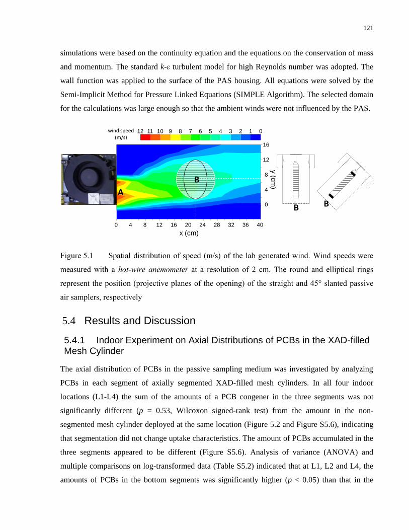
121

simulations were based on the continuity equation and the equations on the conservation of mass

and momentum. The standard k-ε turbulent model for high Reynolds number was adopted. The

wall function was applied to the surface of the PAS housing. All equations were solved by the

Semi-Implicit Method for Pressure Linked Equations (SIMPLE Algorithm). The selected domain

for the calculations was large enough so that the ambient winds were not influenced by the PAS.

Figure 5.1 Spatial distribution of speed (m/s) of the lab generated wind. Wind speeds were

measured with a hot-wire anemometer at a resolution of 2 cm. The round and elliptical rings

represent the position (projective planes of the opening) of the straight and 45° slanted passive

air samplers, respectively


5.4.1 Indoor Experiment on Axial Distributions of PCBs in the XAD-filled Mesh Cylinder

The axial distribution of PCBs in the passive sampling medium was investigated by analyzing

PCBs in each segment of axially segmented XAD-filled mesh cylinders. In all four indoor

locations (L1-L4) the sum of the amounts of a PCB congener in the three segments was not

significantly different (p = 0.53, Wilcoxon signed-rank test) from the amount in the non-

segmented mesh cylinder deployed at the same location (Figure 5.2 and Figure S5.6), indicating

that segmentation did not change uptake characteristics. The amount of PCBs accumulated in the

three segments appeared to be different (Figure S5.6). Analysis of variance (ANOVA) and

multiple comparisons on log-transformed data (Table S5.2) indicated that at L1, L2 and L4, the

amounts of PCBs in the bottom segments was significantly higher (p < 0.05) than that in the

0 4 8 12 16 20 24 28 32 36 40

x (cm)

0123456789101112

0

4

8

12

16

wind speed(m/s)

y (c

m)

A

B

B B

122

middle and top segments. This agrees with a previous study showing a higher PSR of water

when a silica gel filled mesh cylinder was positioned closer to the opening of the sampler

housing.127

L1, L2, and L4 are offices or storage rooms with little activity and thus air turbulence.

Under such wind still condition, the stagnant air layer surrounding the XAD-filled mesh cylinder

farther from the opening of the PAS housing is presumably thicker. Thus a higher chemical

uptake rate applies to the bottom segments of the cylinders than the middle and top segments.

Another possible explanation for the higher uptake rate for the bottom segment is the so-called

“starvation effect”: if the rate of gas diffusion within the housing is smaller than the chemical

uptake rate by the sampling medium, the concentrations of the chemicals in the air surrounding

the middle and top segments could be lower than that in the air surrounding the bottom segment.

A study48

using PUF as the sampling medium observed a decreased PSR when the PUF was

moved further from the opening of the sampler housing. The decreased PSR was partially

attributed to less particles being trapped by a PUF placed further from the opening.48

In the

present study, the congeners with less than 5 chlorines that are predominantly (>95%) in the gas

phase also showed decreased uptake in the middle and top cylinder segments, indicating that

chemical uptake could be limited by gas diffusion within the housing.

Figure 5.2 Amounts of PCBs accumulated in the three axial segments of XAD-resin based

passive air samplers deployed indoors under windy condition generated using electric fans

(L1W1 and L1W2), wind still condition (L1-L4) and deployed outdoors with normal sampler

configuration (ODN), with black painted housings (ODB) and with housings shaded from

sunlight (ODC). The sum of the amounts in the three segments is compared with the amount in a

non-segmented sampler deployed simultaneously at the same location. The whiskers indicate the

root mean square of the distances of the two points to the average.

The amounts of PCBs accumulated in the three segments of the PASs deployed at L3 were not

significantly different (Table S5.2). L3 is an underground cargo loading area with truck traffic

0

10000

20000

30000

40000

50000

60000

70000

80000

90000

L1SW0

10000

20000

30000

40000

50000

60000

70000

80000

90000

L1SW

29%

38%

33%

29%

36%

35%

0

1000

2000

3000

4000

5000

6000

7000

8000

9000

L1SW

0

1000

2000

3000

4000

5000

6000

7000

8000

9000

10

200

400

600

800

1000

L1SW

0

200

400

600

800

1000

1

0

200

400

600

800

1000

L1SW0

200

400

600

800

1000

1

0

200

400

600

800

1000

L1SW

0

200

400

600

800

1000

1

0

200

400

600

800

1000

1200

1400

L1SW

0

200

400

600

800

1000

1200

1400

L1SW

0

200

400

600

800

1000

1200

1400

L1SW

23%

23%

47%

24%

30%

46%

34%

28%

37%

28%29%

43%

30%

34%

36%

33%

31%

37%

27%

33%

41%

L2 L3 L4L1 ODCODN ODB

Σ 15P

CB

am

ou

nt

(μg)

L1W1 L1W2

908070605040302010

0

9876543210

1

0.8

0.6

0.4

0.2

0

1.4

1.2

1.0

0.8

0.6

0.4

0.2

0

123

and other activities; thus air turbulence is expected to be stronger here than the other indoor

locations. Stronger air turbulence may expose the upper segments of the mesh cylinder to wind

to a similar extent as the bottom segments, resulting in similar uptake rates for the three

segments.

Figure 5.3 Masses of PCBs accumulated in the three axial segments of two XAD-resin based

passive air samplers deployed under wind still and lab generated windy conditions

To test whether air turbulence could affect the axial distribution of chemicals in the XAD-filled

mesh cylinder, we set up two electric fans blowing at 45° angle towards the openings of two

PASs with segmented cylinders (Figure S5.2). While the PCB congener profile under these

conditions was similar to that under wind still condition (Figure S5.6), exposure to constant wind

increased the amounts of PCBs accumulated in the PASs ~8 times. The relative difference in the

amounts of PCBs sampled between the duplicates under the windy condition was over 50%,

which was larger than that under wind still conditions. Such large variation is probably caused by

the difficulty of precisely replicating wind patterns; both speed and angle of incidence of the

wind are potential factors varying the uptake rate. In a previous study,20

no differences in the

uptake rate was observed for the same type of PAS with wind blowing at speeds between 5 and

15 m/s. However, the wind was blowing at a straight angle towards the PAS, in contrast to this

preliminary experiment, in which the fans were set up to generate wind at a 45° angle towards

the openings of the PASs.

y = 3.93xR² = 0.992

y = 7.32xR² = 0.995

y = 6.83xR² = 0.995

0

500

1000

1500

2000

2500

3000

3500

0 200 400 600 800

y = 7.63x

R² = 0.987

y = 12.74x

R² = 0.992

y = 13.01xR² = 0.992

0

1000

2000

3000

4000

5000

6000

0 200 400 600 800

PCB mass without wind (ng)

PC

B m

ass

wit

h w

ind

(n

g)

(a) (b)1:1 line

1:1 line

124

Despite of the variations between the duplicates in the absolute PCB amounts accumulated under

lab-generated windy conditions, the relative distribution of PCBs among the three segments was

quite consistent (p = 0.9) (Figure S5.7): No difference in the distributions of PCBs among the

three segments was observed under the lab generated windy condition (Figure S5.8and Table

S5.2).

Comparing the amounts of PCBs accumulated in the segmented cylinders of PASs deployed in

L1 under wind still and windy conditions (Figure 5.3), we note that wind increased the uptake

rates for all three segments of the mesh cylinder (all the points in Figure 5.3 fall on the upper left

side of the 1:1 line). In each segment of the XAD mesh cylinder no statistical difference in the

extent of increase (relative to wind still condition) was found among different PCB congeners

(the points representing different PCB congeners in a segment fall on a line through the origin in

Figure 5.3). Wind increased the uptake rate of the top and middle segments to the same extent

(no significant difference was found between the slopes of the corresponding red and green

regression lines in Figure 5.3; p > 0.4 for the interaction factor in the analysis of covariance;

more detail on the statistical test of the slopes are presented in SI). In both duplicates, the

increase in the uptake rate (the slopes of the lines in Figure 5.3a and b) for the top and middle

segments was ~1.7 times higher than the increase of the uptake in the bottom segments. The

smaller increase of uptake rate for the bottom segments is likely due to them being already

influenced by the air movement in a normal ventilated indoor environment with limited activities.

5.4.2 Outdoor Experiment on Axial Distributions of PCBs in the XAD mesh cylinder

Passive air samplers with axially segmented XAD-filled mesh cylinders in normal housings,

black painted housings and housings shaded from the sunlight were deployed outdoors to test

whether solar radiation would affect chemical uptake and axial distribution in PASs (Figure

S5.3). PCBs accumulating in PASs deployed within and on top of the same building (Figure S5.6)

had similar congener profiles. Even though PSRs tend to be higher outdoors than indoors,127

the

amounts of PCBs accumulated in the PASs deployed at L1 were ~10 times higher than in the

outdoor PASs. This suggests that the building was the source of the PCBs measured on the

building rooftop. This is consistent with previous studies,30,158

which suggested that PCBs are

still continuously emitted from indoor sources.

125

The PASs deployed outdoors showed non-uniform axial distributions of PCBs in the XAD mesh

cylinder (Figure S5.10). This is in contrast with the PASs under the lab generated windy

conditions, in which no statistical differences were observed for the masses of PCBs

accumulated in the three segments of XAD mesh cylinders but similar to the indoor PASs under

wind still condition. During the outdoor deployment segments that are closer to the opening of

the PAS housing generally accumulated more PCBs. The only exception was the middle

segments of the two cylinders deployed in black housings, which both accumulated less PCBs

than the top segment. Different from the wind still indoor conditions where the PCB amounts in

the top segments were 51 ± 2% of that in the bottom segments, the outdoor PASs (normal

housing) showed only a 17 ± 3% decline in the accumulated PCB amount from the bottom to the

top segment. With respect to the axial chemical distributions within the XAD-filled mesh

cylinder, the outdoor deployment falls in between the wind still and artificially windy indoor

deployment.

The total PCB amounts (i.e. sum of amounts in three segments) taken up by the PAS placed in

black housings were no different (Scheffe multiple comparison p = 0.17) from those in shaded

housings, but higher (p < 0.001) than those in normal housings. The shaded housing had more

PCBs (41±1)% in the bottom segments than the normal and black housing, which had (36±1)%

and (37±2)% of PCBs accumulated in the bottom segments. Because all the PASs were deployed

at the same location, they were exposed to the same wind. The lower portion of PCBs

accumulating in the middle and top segments could be caused by less heat convection in the

housing shaded from sunlight. In accordance with expectations, the records of the temperature

loggers (Figure S5.11 and Table S5.3) showed that the black housing experienced the highest

maximum temperatures, followed by the normal housing and the shaded housing. However,

differences were mostly less than 2 °C and occurred only during the day when the samplers were

exposed to direct sunshine. For most of the sampling period, there was no difference in the

temperatures measured in different housings and thus the temperature differences averaged over

the whole sampling period were small (<1°C). No temperature gradients were observed within

any of the sampler housings (Figure S5.12). We conclude that any variation in the PSRs

potentially caused by heat convections is likely so small to be dwarfed by other factors with

greater influence on the kinetics of uptake.

126

5.4.3 Wind Effect on Passive Sampling Kinetics

Calibrations of PASs under lab generated windy and wind still conditions were conducted

indoors to investigate the wind effect on chemical uptake. Similar to the preliminary experiment

(Figure 5.3), uptake of PCBs was faster under windy conditions; wind at a speed of ~4 m/s

increased PSRs ~4-fold (Figure 5.4 and Figure S5.13). This increase in PSRs was smaller than

the 10-fold increase in PSRs observed for the PUF-disk PAS at a wind speed of ~2 m/s

compared to wind still conditions.92

Windy conditions reduce the thickness of the stagnant air

layer, which results in less kinetic resistance to chemical mass transfer and thus elevated PSRs.

The study by Tuduri et al.92

identified a threshold of wind speed (1 m/s) below which wind had

no significant effect on the PSR in PUF-disk PAS. In an earlier experiment measuring water

uptake in a wind tunnel the PSR of the mesh cylinder-PAS did not vary within the wind speed

range from 5 to 15 m/s.20

Based on this, we hypothesize that wind only affect PSRs within

certain ranges of wind speeds. Further studies would be necessary to test the effect of wind on

PSRs at different wind speeds.

Figure 5.4 Passive air sampling kinetics (Penta-CB110 as an example) for samplers under

windy (lab generated wind blowing at 45° slanted angle and at straight angle towards the

cylindrical passive air samplers) and wind still conditions

y = (0.97±0.03)xR2=0.99

y = (0.84±0.03)xR2=0.98

y = (0.25±0.02)xR2=0.93

0

20

40

60

80

100

120

140

160

180

0 40 80 120 160

Windy, Slanted Angle

Windy, Straight Angle

No Wind

Deployment time (d)

Equ

ival

ent

Air

Vo

lum

e (m

3)

127

The ratio between the uptake rates under windy and wind still condition is a measure of the wind

effect. These ratios were 3.8±0.2 and 3.3±0.2 with the wind blowing at a slanted angle and at a

straight angle, respectively. These ratios correlated (r = 0.71, p = 0.003) with the particle bound

fractions if the wind hit the PAS at a slanted angle, but not if the angle of incidence was 90° (p =

0.2). This observation may suggest that a slanted angle of incidence causes more particles to be

trapped in the XAD-filled mesh cylinders. This would be consistent with previous studies on the

PUF-PAS which indicated that wind accelerates particle transfer from air to PUF.87

The PSRs for PCBs under slanted wind conditions were higher than when the wind blew the

PAS at a straight angle (Table S5.4), which agrees with our hypothesis. However, ANCOVA

(see SI) indicated no significant difference in the slopes of the uptake curve (i.e. PSRs) between

the straight and slanted windy conditions for the majority of PCBs congeners (Figure S5.14). In

contrast to a previous study with the PUF-PAS showing a significant influence of the angle of

wind incidence on PSRs,97

observations in this study suggest that this angle has little effect on

the chemical uptake kinetics of the cylindrical XAD-PAS. In the field PASs oftentimes are

subject to highly variable wind conditions due to the effect of local terrain such as a mountain

slope and lack of influence of such variations on PSRs would assist in increasing the precision of

the measurement. Nevertheless, this study only tested two wind directions relative to the PASs,

and further study on wind blowing at other angles is necessary in order to provide more solid

evidence to support this conclusion.

5.4.4 Simulated Wind Conditions in the Sampler

CFD simulations were performed to investigate wind fields in the PASs subject to wind blowing

at straight and at 45° slanted angles towards the PAS. From the simulated wind field at the cross

sections at the bottom, middle and top of the PAS (Figure 5.5), we note the wind speeds were

over 70% lower inside than outside the housing, suggesting the housing largely shields the

sampling medium from the wind. This is consistent with a previous study showing that the

sampler housing dampened the wind and PSR variability in PUF-disk PAS.92

In the PAS with

wind blowing at a straight angle, wind speeds at the top and middle cross sections were similar

but lower than that at the bottom. Wind blowing at 45° angle seems to have more influence on

the wind exposure of the sampling medium within the housings; in particular, the middle and top

cross sections are predicted to have a higher wind exposure than if the wind is blowing at the

128

PAS at a straight angle. Nevertheless, the differences in the wind speeds within the housing of

PAS subjected to straight and slanted wind are predicted to be small, which probably explains

the non-significant difference in the PSRs between the two wind conditions.

Figure 5.5 Computational fluid dynamic simulations of wind field on the cross sections at the

top (a and d), middle (b and e) and bottom (c and f) of the XAD mesh cylinders within the

housing of the passive air samplers subject to wind blowing at straight (a-c) and at 45° slanted

angles (e-f) towards the sampler

5.4.5 Implications and Further Research Questions Originating From This Study

The present study shows that wind would increase the PSRs and reduce the non-uniform axial

distributions of chemicals in the cylindrical sampling medium of the XAD-PAS. When applying

PASs under less windy conditions such as indoors, PSRs obtained in outdoor calibration studies

are unlikely to be valid; PAS will need to be recalibrated for use under conditions with limited

air turbulence. Higher PSR induced by wind allow for shorter PAS deployment times, if the

sampled chemicals are close to the detection limit. Windy conditions also tend to reduce the non-

uniform uptake by the sampling medium at different distances from the opening of the housing.

0 1 2 3 4 5Wind speed (m/s)

(a)

(b)

(c)

(d)

(e)

(f)

129

However, the influence of wind on PSRs can introduce large uncertainty to PAS-derived air

concentrations. Therefore, optimization of PAS design would seek to minimize the influence of

wind (e.g. by covering the opening of the housing with a fine mesh screen) while maximizing the

PSR by varying other factors that are independent of environmental conditions (e.g. the

configuration of the sampling medium). The results of this study show a significant increase in

PSRs between wind-still conditions and wind speeds of ~4m/s while an earlier study indicated no

significant change of PSRs when ambient wind speeds increased from 5 to 15 m/s. This suggests

that the wind effect on PSRs may depend on the wind speed range. As such, further studies on

the wind effect on the PSRs at different wind speeds are worthwhile to fill this knowledge gap.

5.5 Acknowledgments


Sciences and the Natural Sciences and Engineering Research Council of Canada. XZ also

acknowledges financial support by an Ontario Graduate Scholarship.

130


Figure S5.1 Passive air samplers with axially segmented XAD-filled mesh cylinder to study

the axial chemical distribution within the sampling medium.

Figure S5.2 Experiment setup to study chemical distributions in the axially segmented passive

sampling medium (XAD mesh cylinder) under wind and wind still conditions.

131

Figure S5.3 Experiment setup to study potential effect of solar radiation on chemical uptake

and axial distribution within the XAD mesh cylinder.

132

Figure S5.4 Experiment setup to study potential wind effects on chemical uptake by the XAD

passive air sampler.

Figure S5.5 Variations of wind speed measured at the mouth of the fans (point A of Figure 1)

and at the openings of the sampler housings (point B of Figure 1) for the 24 passive air samplers

subjected under lab generated windy conditions.

2.5

3

3.5

4

4.5

5

5.5

6

11.0 11.5 12.0 12.5 13.0 13.5

12.0 ± 0.4

4.3 ± 0.2

3.6 ± 0.3

11.8 ± 0.4

Wind speed at the mouth of the fan (m/s)

Win

d s

pee

d a

t th

e m

ou

th o

f th

e PA

S (m

/s)

133

Table S5.1 Target ions, quanlify ions and limit of detection (LOD) of the PCB homolog

groups analyzed using GC-MS selected ion monitoring mode.

a LOD calculated as the chemical amount of which the instrument detects a signal corresponding

to three times of the noise level.

Class Chemical Target

Ion

Qualify

Ion

(Qual. /Targ.)

*100%

LOD a

(ng/sample)

Internal Standard Mirex 272 274 81.1 n/a

Surrogate Standard 13CPCB77 304 302 77.2 n/a


Surrogate Standard 13CPCB141 372 374 81 n/a


Target Analyte Tri-CB 256 258 98 0.5

Target Analyte Tetra-CB 292 290 76.7 1

Target Analyte Penta-CB 326 328 65.3 0.2

Target Analyte Hexa-CB 360 362 81.4 1.5

134

Figure S5.6 Amounts of PCBs accumulated in the three axially segment3ed passive air

sampling medium (XAD mesh cylinder) of passive air samplers deployed in the four indoor

locations (L1-4), passive air samplers with lab generated wind (L1W), and at outdoor location

(OD)

0

400

800

1200

1600

0

20

40

60

80

100

120

0

50

100

150

200

0

20

40

60

80

100

0

50

100

150

200

250

L1

L2

OD

L3

L4

Am

ou

nt o

f P

CB

s a

ccu

mu

late

d in

th

e p

ass

ive

sam

pli

ng

med

ium

(ng)

PCB congener

(a)

(f)

(d)

(c)

(b)

0

2000

4000

6000

8000

10000

12000

14000(e) L1W

135


duplicated PASs blown with lab generated wind.


duplicated PASs (a) under the quasi wind still condition; (b) under the lab generated windy

condition; (c) in outdoor environment

0%

20%

40%

60%

80%

100%

0%

20%

40%

60%

80%

100%

Per

cen

t of

PC

Bs

acc

um

ula

ted

PCB congener

Perc

enta

ge o

f PC

Bs

accu

mu

late

d in

eac

h s

egm

ent

PCB congener

(a)

(b)

(c)

0%

20%

40%

60%

80%

100%

0%

20%

40%

60%

80%

100%

31

/28

52

49

44

74

66

95

10

1

99

87

11

0

11

8

14

9

15

3

13

8

0%

20%

40%

60%

80%

100%

31

/28

52

49

44

74

66

95

10

1

99

87

11

0

11

8

14

9

15

3

13

8

136

Table S5.2 Two-factorial ANOVA and Scheffé's post hoc test on the PCB congeners

accumulated at the three axially segmented PSM

Sample

ANOVA on ln-transformed PCB amount

Scheffé's Post Hoc Test

SS df MS F p

B M T

L1

PSM Segment 8.0 2.0 4.0 148.8 0.000

B

<0.001 <0.001

PCB Congener 63.6 14.0 4.5 169.2 0.000

M <0.001

<0.001

Segment * Congener 0.0 28.0 0.0 0.0 1.000

T <0.001 <0.001

B M T

L1_Wind

PSM Segment 0.9 2.0 0.5 2.5 0.092

B

0.774 0.342

PCB Congener 64.4 14.0 4.6 24.9 0.000

M 0.774

0.1


T 0.342 0.1

B M T

L2

PSM Segment 7.0 2.0 3.5 70.9 0.000

B

<0.001 <0.001

PCB Congener 48.7 14.0 3.5 70.6 0.000

M <0.001

<0.001


T <0.001 <0.001

B M T

L3

PSM Segment 1.2 2.0 0.6 9.9 0.000

B

<0.001 0.209

PCB Congener 42.7 14.0 3.1 49.1 0.000

M <0.001

0.04


T 0.209 0.04

B M T

L4

PSM Segment 2.4 2.0 1.2 36.6 0.000

B

<0.001 <0.001

PCB Congener 39.9 11.0 3.6 111.4 0.000

M <0.001

0.787


T <0.001 0.787

B M T

OD

PSM Segment 0.5 2.0 0.2 79.6 0.000

B

<0.001 <0.001

PCB Congener 42.5 14.0 3.0 1034.8 0.000

M <0.001

<0.001


T <0.001 <0.001

B M T

OD_Black

PSM Segment 2.7 2.0 1.4 197.1 0.000

B

<0.001 <0.001

PCB Congener 42.2 14.0 3.0 432.4 0.000

M <0.001

<0.001


T <0.001 <0.001

B M T

OD_Covered

PSM Segment 0.5 2.0 0.2 177.9 0.000

B

<0.001 <0.001

PCB Congener 44.2 14.0 3.2 2428.6 0.000

M <0.001

<0.001


T <0.001 <0.001

137

Testing the slopes of two linear regressions using analysis of covariance (ANCOVA).

ANCOVA Model: ( ) i j i ij i j

Y A X X

i jY : The value of the response variable for the jth observation in the ith treatment of factor A

: The overall mean value of the response variable

iA : The effect of the ith treatment of factor A, defined as the difference of the mean of each A

and the overall mean ( i i

A )

: A combined regression coefficient representing the pooling of the regression slopes of Y on

X within each group.

ijX : Covariate value for the jth replicated observation from the ith level of factor A

X : mean value of covariate

i j

: Unexplained error associated with jth replicate observation from the ith level of factor A

Null hypothesis to test the slopes of regression lines (H0): no difference between the regression

coefficients under treatment of A1, A2…Ai (i.e.1 2

... i)

When the interaction effect between the treatment factor A and the covariate in the ANCOVA

model is significant, the effect the covariate on the response depends on the treatment factor,

which means the slopes of regressions for each treatment factor are not statistically the same and

H0 is rejected.

138

Figure S5.9 Mass of PCBs accumulated in the three axially segmented passive air sampling

medium (XAD mesh cylinder) of passive air samplers deployed outdoors (a) under normal

condition (b) with black sampler housing and (c) with black sampler housing shaded from direct

sunshine.

0

50

100

150

200

250

0

50

100

150

200

250

0

50

100

150

200

250

PCB

am

ou

nt a

ccu

mu

late

d (n

g)

PCB congener

(a)

(b)

(c)

139


normal housings, back housings and housings shaded from sunshine.

0%

20%

40%

60%

80%

100%

0%

20%

40%

60%

80%

100%

0%

20%

40%

60%

80%

100%Perc

ent o

f PC

Bs

accu

mu

late

d

PCB congener

140

Table S5.3 Descriptive statistics on the temperature (°C) recorded by the temperature logger

in the passive air samplers deployed outdoors

Logger position in the

passive air sampler

Logger recorded temperature (°C)

A B C D E F G H I

Max 49.0 50.5 49.5 43.0 45.5 45.0 37.0 38.5 39.0

75%ile 22.0 22.0 21.5 21.5 21.5 21.5 20.5 20.5 21.0

Mean 16.8 16.9 16.9 16.8 16.8 16.4 15.7 16.0 16.4

Median 15.5 15.5 15.5 15.5 15.5 15.5 15.0 15.5 15.5

25%ile 10.5 10.5 11.0 11.5 11.0 11.0 11.0 11.0 11.5

Min -2.5 -2.5 -1.5 -1.5 -1.5 -1.5 -1.5 -1.0 -1.0

Outer wall

of PAS housing painted

black

Sun shelter

Temperature

logger

I

H

G

F

E

D

C

B

A

141

Figure S5.11 Temperature differences in the normal, black, and shaded passive sampler

housing.

-2 0 2 4 6 8 10 12 140

200

400

600

Y A

xis

Title

X Axis Title

BlackT-CovT

-2 0 2 4 6 8 10 12 140

200

400

600

Y A

xis

Title

X Axis Title

BlackM-CovM

-2 0 2 4 6 8 10 12 140

200

400

600

Y A

xis

Title

X Axis Title

BlackB-CovB

-2 0 2 4 60

200

400

600

800

Y A

xis

Title

X Axis Title

BlackT-NormT

-2 0 2 4 60

200

400

600

800

Y A

xis

Title

X Axis Title

BlackM-NormM

-2 0 2 4 60

200

400

600

800

Y A

xis

Title

X Axis Title

BlackB-NormB

-2 0 2 4 6 8 100

200

400

600

800

1000

Y A

xis

Title

X Axis Title

NormT-CovT

-2 0 2 4 6 8 100

200

400

600

800

1000

Y A

xis

Title

X Axis Title

NormM-CovM

-2 0 2 4 6 8 100

200

400

600

800

1000

Y A

xis

Title

X Axis Title

NormB-CovB

Black - Normal Normal-Covered Black - Covered

Top

Middle

Bottom

Top

Middle

Bottom

Top

Middle

Bottom

Temperature Difference (°C)

Nu

mb

er o

f O

bse

rvat

ion

Bottom

Middle

Top

142

Figure S5.12 Comparison of temperatures (°C) at different positions within the passive air

sampling housing.

y = 0.97x

-5

5

15

25

35

45

-5 0 5 10 15 20 25 30 35 40 45

y = 1.00x

-5

5

15

25

35

45

-5 0 5 10 15 20 25 30 35 40 45

y = 0.97x

-5

5

15

25

35

45

-5 0 5 10 15 20 25 30 35 40 45

y = 1.02x

-5

5

15

25

35

45

-5 0 5 10 15 20 25 30 35 40 45

y = 1.04x

-5

5

15

25

35

45

-5 0 5 10 15 20 25 30 35 40 45

y = 1.02x

-5

5

15

25

35

45

-5 0 5 10 15 20 25 30 35 40 45

y = 1.01x

-5

5

15

25

35

45

-5 0 5 10 15 20 25 30 35 40 45

y = 0.99x

-5

5

15

25

35

45

-5 0 5 10 15 20 25 30 35 40 45

y = 0.98x

-5

5

15

25

35

45

-5 0 5 10 15 20 25 30 35 40 45

Sun shelter

I

H

G

F

E

D

C

B

A

A

B

A

C

B

C

D

E

D

F

E

F

G

H

G

I

H

I

143

Figure S5.13 Passive air sampling kinetics for samplers under windy (lab generated wind

blowing at 45° slanted angle and at straight angle towards the cylindrical passive air samplers)

and wind still conditions.

y = 0.49xy = 0.44x

y = 0.13x0

10

20

30

40

50

60

70

80

90

0 40 80 120 160

TriCB31/28

y = 0.64xy = 0.58x

y = 0.17x0

20

40

60

80

100

120

0 40 80 120 160

TetraCB52

y = 0.75xy = 0.65x

y = 0.20x0

20

40

60

80

100

120

140

0 40 80 120 160

TetraCB49

y = 0.58xy = 0.50x

y = 0.16x0

20

40

60

80

100

120

0 40 80 120 160

TetraCB44

y = 0.74xy = 0.65x

y = 0.19x0

20

40

60

80

100

120

140

0 40 80 120 160

PentaCB95

y = 0.92xy = 0.81x

y = 0.24x0

20

40

60

80

100

120

140

160

180

0 40 80 120 160

TetraCB66

y = 0.81xy = 0.70x

y = 0.21x0

20

40

60

80

100

120

140

160

0 40 80 120 160

PentaCB101

y = 0.67xy = 0.58x

y = 0.17x0

20

40

60

80

100

120

0 40 80 120 160

PentaCB99

y = 0.85xy = 0.74x

y = 0.22x0

20

40

60

80

100

120

140

160

0 40 80 120 160

PentaCB87

y = 0.97xy = 0.84x

y = 0.25x0

20

40

60

80

100

120

140

160

180

0 40 80 120 160

PentaCB110

y = 0.94xy = 0.81x

y = 0.24x0

20

40

60

80

100

120

140

160

180

0 40 80 120 160

HexaCB149

y = 1.21xy = 1.05x

y = 0.32x0

50

100

150

200

250

0 40 80 120 160

HexaCB118

y 1.00xy = 0.82x

y = 0.26x0

20

40

60

80

100

120

140

160

180

0 40 80 120 160

TetraCB74

y = 1.21x

y = 1.00x

y = 0.29x0

50

100

150

200

250

0 40 80 120 160

HexaCB153

y = 1.35xy = 1.16x

y = 0.33x0

50

100

150

200

250

0 40 80 120 160

HexaCB138

Deployment time (d)

Equ

ival

ent

Air

Vo

lum

e (m

3)

144

Table S5.4 Passive sampling rates (PSRs) derived as the slopes of the regressiona between

the deployment time and equivalent sampling volume.

Windy, Slanted Angle

Windy, straight

no wind

PCB congener PSR (m3/d) SE b R2 c

PSR (m3/d) SE R2

PSR (m3/d) SE R2

TriCB31/28 0.49 0.02 0.98

0.44 0.02 0.99

0.13 0.01 0.93

TetraCB52 0.64 0.02 0.99

0.58 0.02 0.98

0.17 0.01 0.94

TetraCB49 0.75 0.03 0.98

0.65 0.02 0.99

0.20 0.02 0.93

TetraCB44 0.58 0.02 0.98

0.50 0.02 0.98

0.16 0.01 0.93

TetraCB74 1.00 0.04 0.99

0.89 0.04 0.98

0.26 0.02 0.95

TetraCB66 0.92 0.03 0.99

0.81 0.03 0.99

0.24 0.02 0.92

PentaCB95 0.74 0.03 0.99

0.65 0.02 0.98

0.19 0.02 0.94

PentaCB101 0.81 0.03 0.99

0.70 0.03 0.99

0.21 0.02 0.94

PentaCB99 0.67 0.03 0.98

0.58 0.02 0.98

0.17 0.01 0.93

PentaCB87 0.85 0.03 0.99

0.74 0.03 0.98

0.22 0.02 0.93

PentaCB110 0.97 0.03 0.99

0.84 0.03 0.98

0.25 0.02 0.93

HexaCB149 0.94 0.03 0.99

0.81 0.03 0.98

0.24 0.02 0.93

PentaCB118 1.21 0.05 0.98

1.05 0.03 0.99

0.32 0.03 0.93

HexaCB153 1.21 0.05 0.98

1.00 0.04 0.98

0.29 0.03 0.92

HexaCB138 1.35 0.04 0.99

1.16 0.05 0.98

0.33 0.03 0.93

a regression forced through the origin

b Standard error of the regression coefficients (PSRs)

c For regression through the origin (the no-intercept model), R

2 measures the proportion of the

variability in the dependent variable explained by regression. This cannot be compared to R2 for

models which include an intercept

145

Figure S5.14 (a) Passive air sampling rates of PCBs under quasi wind still condition and with

lab generated wind blowing at straight and 45° slanted angles towards the passive air samplers;

(b) statistical test on the difference of passive air sampling rates between the two windy

conditions.

0.00.20.40.60.81.01.21.4

0

0.05

0.1

0.15

0.2

PCB congener

PSR

(m3/d

)P

valu

e

(a)

(b) PSR difference betweentwo windy conditions

significant

non-significant

146

Chapter 6. Application of passive air samplers and flow-through air samplers to assess semi-volatile organic contaminants in the atmosphere of

Hawaii

Xianming Zhang, John Barnes, Ying D. Lei, Frank Wania

Contributions: F. Wania and X. Zhang planned the sampling campaign. X. Zhang did the field

work with the assistance of J. Barnes, J. Armitage, and A. Gawor. X. Zhang extracted the

samples, performed analysis using GC/MS/MS under the guidance of Y.D. Lei, and processed

the chromatograms. X. Zhang interpreted the data and wrote the manuscript with the guidance of

F. Wania.

147

6.1 Abstract

An air sampling campaign using passive air samplers (PASs) and flow-through samplers (FTSs)

for semivolatile organic compounds (SVOCs) was conducted on the Big Island of Hawaii with

the purpose to (1) test the potential starvation effect of PASs in the field, (2) explore the vertical

distribution of SVOCs along an altitudinal transect, and (3) assess global SVOC background

concentrations over the Central Northern Pacific. XAD-resin based PASs were deployed from

May to September 2011 at six sites along a transect from the northeastern coast to the Mauna

Loa Observatory 3400 m above sea level and at three control sites on the island. By crossing the

trade wind inversion layer the transect ranged from the marine boundary layer to the free

troposphere. At the two ends of the transect, FTSs were deployed to simultaneously sample air at

monthly resolution. Based on a comparison of the amounts of polycyclic aromatic hydrocarbons

(PAHs) and polybrominated diphenyl ethers (PBDEs) accumulated in differently configured

PAS deployed side-by-side, the starvation effect was judged insignificant, i.e. the kinetic

resistance for chemical transfer from ambient air into the sampler housing had no significant

influence on overall chemical uptake. Elevated PAHs and PBDEs levels at two sites close to Hilo

indicated contributions of local sources to the SVOCs in air. SVOC concentrations decreased

with increasing elevation. Higher rates of decrease for PAHs than for PBDEs correspond to

higher atmospheric degradation rates of PAHs than PBDEs. Levels of PAHs and PBDEs at the

Mauna Loa Observatory were generally at the lower end of the range of concentrations reported

at other remote sites, including the Arctic. However, in contrast to the Arctic, long range

atmospheric transport is deemed less important than human-induced material flow as the source

of the SVOCs to the island’s atmosphere. The latter process would be important in the chemical

life cycle impact assessment for environments such as isolated tropical islands.

6.2 Introduction

Semivolatile organic chemicals (SVOCs) such as polybrominated diphenyl ethers (PBDEs),

polycyclic aromatic hydrocarbons (PAHs) have attracted great concerns because of their

potential hazard to environment and humans.30,66,159,160

Some SVOCs (e.g. PBDEs) were

produced intentionally for enhancing the function of commercial products while others (e.g.

PAHs) are generated from natural or anthropogenic processes such as combustion. Due to

national and international regulations on some SVOCs, re-volatilization from soils and oceans is

148

gaining in importance relative to primary emissions to the atmosphere.161

Upon entering the

atmosphere, SVOCs are prone to undergo long range atmospheric transport to remote regions

where local emissions are low. Global atmospheric transport of SVOCs mainly occurs in the free

troposphere (FT) due to higher wind speeds and limited exchange with the earth’s surface.162,163

As such, investigating the occurrence of SVOCs in the FT is important for understanding

atmospheric transport of SVOCs to remote regions.163

Due to the difficulty of accessing

sampling sites, much fewer measurements of SVOCs have been conducted in the FT than the

planetary boundary layer. Such measurements were mainly conducted from aircraft164,165

or at

high mountain sites,160,163,166

and most have been conducted over the continents. Only a few have

focused on SVOCs in the FT over the oceans by sampling high altitude sites on an island.163

SVOCs in air are conventionally sampled using high-volume active air samplers

(HVAASs),167,168

which are able to provide high temporal resolution and information on

gas/particle partitioning.108,163,169

However, HVAASs require electricity and frequent operator

visits and are difficult and expensive to deploy at multiple sites to study the spatial variations of

SVOCs in the air of remote regions.108

Overcoming these disadvantages, passive air samplers

(PASs) are increasingly used to obtain time-integrated SVOC air concentrations in various types

of environment.42,72,154

PASs are especially useful in providing high spatial resolution data to

elucidate the fate of SVOCs in remote regions such as mountains.34,37,166,170-172

Although PASs

have many advantages and have been widely used, passive sampling rates (PSRs) are potentially

influenced by many factors. Understanding these factors is necessary in order to properly

interpret and compare PAS-derived air concentrations. A few studies have investigated

potentially influential factors such as wind, temperature, properties of the target chemicals, and

sampler configuration.89,90,97,127

A question arose from our previous study:126

Does a starvation

effect exist and does it affect PSRs of the XAD-resin based PASs? This effect refers to lower

concentrations of target chemicals within the PAS housing than in ambient air, which would

occur if the uptake of chemicals by the sampling medium is faster than the rate of transfer from

ambient air into the PAS housing. So far, the existence of such an effect has not been tested in

the field.

While time-integrated sampling is an advantage of PASs, the PSRs are generally low (< 5 m3/d)

so that PASs have to be deployed from several months to a year in order to allow for the

detection of the accumulated chemicals. To overcome the limitation of low temporal resolution

149

while keeping other advantages of PASs, a flow-through sampler (FTS) was developed to sample

SVOCs in air.45

The FTS consists of a horizontally oriented flow tube, which turns into the wind

with the help of vanes. It relies on the wind to pass air through a plug of polyurethane foam that

serves as the sampling medium. Such a design can increase the sampling rate (> 15 m m3/d) and

has proven useful for monitoring SVOCs in remote areas with a much higher temporal resolution

than PAS.46

In this study, an air sampling campaign using PASs and FTSs was conducted on the Big Island

of Hawaii with the aim to (1) test the potential starvation effect on PASs ; (2) explore the vertical

variations of SVOCs from sea level to the top of the Mauna Loa volcano, (3) assess the

occurrence of several groups of SVOCs in the FT over the central northern Pacific and compare

their concentrations with those in the marine boundary layer.

Figure 6.1 Locations of the sampling sites on the Big Island of Hawaii. A-I: passive air

samplers; A and F: flow-through air samplers.


6.3.1 Sampling Sites

Located in the Central Northern Pacific, the archipelago of Hawaii is a relatively easily accessed

place far from the continents (>3000 km). The air sampling campaign was conducted on the Big

Island of Hawaii, which is a volcanic island covering 10,432 km2.173,174

Less than 1.5 million

150

people live within a 3000 km radius of the island, which itself has a population of 185,000.29

The

elevation on the island rises by more than 3000 m over a horizontal distance of less than 60 km.

Prevailing northeasterly trade wind bring marine air to the island. A persistent trade wind

inversion caps the atmospheric planetary boundary layer at approximately 2000 m above sea

level.175

6.3.2 Sampling Campaign

Cylindrical PASs using XAD-resin filled mesh cylinder as the passive sampling medium (PSM)

were deployed to conduct time-integrated sampling at nine sites (labeled A-I in Figure 6.1) from

May to September, 2011. Six of these sites form a transect from the northeastern coast (Site A,

elevation: 0 m) to the Mauna Loa Observatory (Site F, elevation: 3400 m) and extend from the

planetary boundary layer (sites A-D) to the FT (sites E and F). For comparison PAS were also

deployed at sites on the east end of the island (G), in Volcano Village (H), and in the northeast of

the island (I). Two FTSs were deployed at sites A and F to sample air at a monthly temporal

resolution during the PAS deployment period. Detailed information on the location and elevation

of the sampling sites is given in Table S6.1 of the Supporting Information (SI).

At each of the sites (except A and H) three XAD-PASs (Figure S6.1) were deployed: a long one,

a short one and a short one with two XAD-resin filled mesh cylinders in one housing. By

comparing the amounts of SVOCs accumulated in three differently configured PASs deployed

side-by-side, we aimed to probe the existence of a starvation effect. At each site, a temperature

logger (ACR System Inc.) was mounted in a PAS housing to record the temperatures during the

sampling period (Figure S6.2).

Pre-extracted XAD resin used in the PASs was cleaned by Soxhlet extractions with acetone for

24 h and with hexane for another 24h. Polyurethane foam (PUF) plugs used in the FTSs were

cleaned up by tap water and deionized water and then Soxhlet extracted with acetone for 24 h

and with petroleum ether for another 24h. XAD-resin filled mesh cylinders were sealed in pre-

cleaned stainless steel tubes and PUF plugs were stored in pre-cleaned air tight glass jars before

being used in the field. Upon retrieval, each XAD-filled mesh cylinder and each PUF plug was

separately placed in their original containers and stored in a freezer in Hilo, Hawaii before being

transported to a freezer in the lab in Toronto at the end of the sampling campaign. The samples

151

from the FTSs and from the PASs were extracted within one month and three months of retrieval,

respectively.

6.3.3 Sample Extraction

Prior to extraction, each sample was spiked with 100 μL of isotope-labeled standards. Identities

and concentrations of those standards are listed in Table S6.2. The XAD-resin was extracted by

accelerated solvent extraction (Dionex ASE-350) using 33 or 66 ml cells for the short and long

mesh cylinders, respectively. The ASE conditions followed a methods previously used in our

lab127,149

: solvent 50:50 hexane:acetone; temperature 75°C; pressure 1500 psi; static time 5 min;

static cycles 3; flush volume 100%; purge time 240 s. The PUF plugs were Sohlet extracted with

petroleum ether for 24 h. After extraction, each extract was roto-evaporated to ~2 mL and

filtered through ~1 g of anhydrous sodium sulfate packed in a disposable pasteur pipet to remove

moisture. The eluent was solvent exchanged to isooctane, blown down with high purity nitrogen,

transferred to a GC vial, and further reduced to 0.5 mL. To the GC vial, 10 μL of 10 ng∙μL-1

mirex and 20 μL of 1 ng∙μL-1

each of BDE-75, 116, 205 were added to quantify the recovery of

the surrogates.

6.3.4 Sample Analysis

Both PAHs and PBDEs were analyzed using an Agilent 7890A gas chromatography (GC)

coupled to an Agilent 7000A triple quadrupole mass spectrometry (MS/MS) with EI source. For

PAH analysis, 1.0 μL of the sample was injected in splitless mode with the injector temperature

at 250 °C. PAHs in the sample were separated using a J&W HP-5MS column (30m × 250 μm ID

× 0.25 μm film thickness) with helium (1.2 mL/min) as the carrier gas. The column temperature

program started from 90 °C for 1 min, to 250 °C at 10 °C·min-1

, to 300 °C at 5 °C·min-1

, and held

for 3 min. The interface, source and quadrupole temperatures were set at 250 °C, 230 °C and

150°C, respectively. For PBDE analysis, 2.0 μL of the sample was injected in splitless mode

with the injector temperature at 285 °C. PBDEs in the sample were separated using a J&W HP-

5MS column (15m × 250 μm ID × 0.25 μm film thickness) with helium (1.8 mL/min) as the

carrier gas. The column temperature program started from 100 °C, to 185 °C at 25 °C·min-1

, to

275 °C at 15 °C·min-1

, to 315 °C at 45 °C·min-1

, and held for 6 min. The interface, source and

quadrupole temperatures were set at 300 °C, 230 °C and 150 °C, respectively. Both PAHs and

PBDEs were detected using multiple reaction monitoring (MRM) mode with He (2.25 mL/min)

152

as the quench gas and N2 (1.5 mL/min) as the collision gas. The precursor ions, product ions and

collision energies selected and monitored for PAH analysis are listed in Table S6.3. Those for

PBDE analysis are listed in Table S6.4.

6.3.5 QA/QC

Field blanks were collected by exposing the sampling medium to the air at the sampling sites for

1 min and by storing and transporting them the same way as the samples until analysis. 8 field

blanks of the XAD-filled mesh cylinder were collected. 10 field blanks (1 for each site every

month) were originally planned for the FTSs during the whole sampling campaign. However,

two glass jars were broken while being transported to the field so the number of field blanks for

the FTSs was reduced to 8. Of the PAHs and PBDEs analyzed, only fluorene and phenanthrene

can be detected in the blanks for the FTSs. The blank levels (1-10 ng/sample) were <5% for 90%

of the samples and <10% for all the samples. The reported data were not blank corrected.

Recoveries of the isotope labeled standards spiked prior to extraction were 60-148% PAHs and

56-121% for PBDEs. The reported data were recovery corrected.

6.3.6 Air Mass Back Trajectory Analysis

The origins of air masses arriving at sampling sites A and F were assessed via back trajectories

calculated using the hybrid single-particle Lagrangian integrated trajectory (HYSPLIT) model.176

Based on the Global Data Assimilation System (GDAS) 1 degree latitude longitude

meteorological dataset, 14 d back trajectories for air masses arriving at 50 m above ground of the

two sites were calculated every 6 h for the entire sampling period. The point densities of

endpoints of the trajectories were derived and mapped using the spatial analysis tool of ArcGIS

10.0.


6.4.1 PAHs and PBDEs Accumulated in PASs of Different Configuration

Deploying side-by-side a short PAS with two 10-cm-long XAD filled mesh cylinders, a short

PAS with one 10-cm-long XAD filled mesh cylinder and a long PAS with one 20-cm-long XAD

filled mesh cylinder (Figure S6.2), we intended to test the existence of starvation effect of the

XAD-PAS, i.e. whether the rate of uptake by the PSM is faster than the rate of chemical transfer

from ambient air into the sampler housing.

153

Figure 6.2 Comparison of the amounts (ng) of chemicals (fluorene, phenanthrene,

fluoranthene, pyrene, BDE47and BDE99) sampled by PASs of different configurations.

Had the starvation existed, the amounts of SVOCs accumulated in each of the two short XAD

filled mesh cylinders placed in a single housing of PAS would be less than the SVOC amounts

sampled by the PAS with only one short XAD-filled mesh cylinder. No such difference was

observed (Figure 6.2a, Wilcoxon signed ranks test, p = 0.17), indicating that chemical transfer

from ambient air to housing (i.e. the resistance posed by the sampler housing) does not

kinetically limit the PSRs of PASs deployed under general outdoor conditions.

Previous studies had indicated that PSRs for the cylindrical XAD-PAS deployed outdoors are

lower than those of the double-bowl shaped PAS using PUF as the PSM.108

The different design

of the sampling housings is one possible cause for different PSRs between the two PASs. The

PSM is more confined in the cylindrical sampler housing of the XAD-PAS than in the double-

bowl housing of the PUF-PAS, which could limit chemical uptake kinetics. Our results indicate

that the cylindrical sampling housing poses no significant kinetic limit on the outdoor PSRs. This

adds merit to the cylindrical PAS housing design because the PSM in such a housing is less

susceptible to the influence of wind than in the double-bowl housing.96

Since a higher influence

of wind on chemical uptake by the PSM adds uncertainty to PSRs,93,118

an ideal PAS housing

design would seek to minimize the wind exposure of the PSM without adding to the overall

kinetic resistance to chemical transfer from ambient air to PSM. Even if we found that outdoors

the PSR is not limited by the cylindrical sampling housing, we cannot infer that this is also the

case in an indoor environment. Lower air turbulence is likely to increase the kinetic resistance

for chemical transfer from ambient air to the inside of the sampler housing. Therefore, similar

0

10

20

30

0 10 20 30

0

5

10

15

0 5 10 15

p=0.17

(a)

0

10

20

30

0 10 20 30

p=0.51

(c)

2 ×

(b)

p=0.64

154

experiments should be conducted indoors to test whether kinetic resistance from the sampler

housing is important under conditions of low air turbulence.

The amounts of SVOCs sampled by the long XAD-PASs were double of those sampled by the

short ones (Figure 6.2b). This implies that under outdoor conditions, no additional uncertainty is

introduced when applying PSRs obtained from calibrations with one type of XAD-PAS to the

other by simply dividing or multiplying the PSRs by two. Because no starvation effect existed,

the amounts of SVOCs sampled by the long PAS did not differ (p = 0.51) from the sum of the

two short XAD-filled mesh cylinders put in one sampler housing (Figure 6.2c). This was

expected as the same interfacial transfer area between the PSM and surrounding air, which

determines the PSR, was the same.127

This result validates our proposed approach for improving

the PAS design:127

instead of using a single piece of PSM in a large PAS housing, several

smaller pieces can be positioned in a smaller PAS housing, which would reduce the expense of

making and shipping large PAS housings without reducing the interfacial transfer area between

the PSM and the surrounding air, and thus also the PSR.

This result also implies that air samples can be duplicated (or triplicated) by putting two (or three)

XAD-filled mesh cylinders in one sampler housing. Again, this could reduce the expenses of

shipping PAS housings to remote field sites. Note that with a larger amount of additional PSM in

a sampler housing the rate of chemical uptake by the PSM may increase and eventually exceed

the rates of chemical transfer from ambient air to the inside of the sampler housing, resulting in a

starvation effect. The maximum amount of PSM that can be used in a single sampler housing

under different environmental conditions without causing a starvation effect remains to be

established.

6.4.2 Passive Air Sampler Derived Spatial Variations of PAHs and PBDEs

Large spatial variations of the XAD-PAS-derived levels (ng/PAS) of PAHs and PBDEs were

observed. The highest PAH levels were found at sampling site A (Figure 6.3a), which is at the

northeastern coast of the island and faces the northwestern Pacific Ocean. Although the

population density around site A is lower than that around site B located in the urban area of Hilo,

Hilo airport is ~1000 m south, a wharf with petroleum refinery facilities is ~600 m west and a

beach park is ~200 m northeast of site A. As petroleum and other fuel combustion could be

155

sources of PAHs, these facilities around site A could possibly contribute to the ~50% higher

PAHs levels at site A than at site B. PAH levels at site A were ~30 times higher than that at site

G, another coastal site ~40 km southeast of site A. The difference between the two coastal sites

indicates PAHs measured at site A were mainly from local sources around site A, instead of from

the marine boundary layer.

Figure 6.3 Spatial distributions of (a) polyaromatic hydrocarbons (PAHs) and (b)

polybrominated diphenyl ethers (PBDEs) sampled by passive air samplers (20 cm long XAD

filled mesh cylinder) on the Big Island of Hawaii. Dash lines indicate the altitude of the sampling

sites.

0

500

1000

1500

2000

2500

3000

3500

Alt

itu

de(m

)0.0

50.0

100.0

150.0

200.0

250.0

Pyrene

Fluoranthene

Phenanthrene

Fluorene

0

20

40

60

80

PAHs

(ng/PAS)

0.0

50.0

100.0

150.0

200.0

250.0

Pyrene

Fluoranthene

Phenanthrene

Fluorene

0.0

50.0

100.0

150.0

200.0

250.0

Pyrene

Fluoranthene

Phenanthrene

Fluorene

0.0

50.0

100.0

150.0

200.0

250.0

Pyrene

Fluoranthene

Phenanthrene

Fluorene

0.0

50.0

100.0

150.0

200.0

250.0

Pyrene

Fluoranthene

Phenanthrene

Fluorene

0.0

50.0

100.0

150.0

200.0

250.0

Pyrene

Fluoranthene

Phenanthrene

Fluorene

0.0

50.0

100.0

150.0

200.0

250.0

Pyrene

Fluoranthene

Phenanthrene

Fluorene

0.0

50.0

100.0

150.0

200.0

250.0

Pyrene

Fluoranthene

Phenanthrene

Fluorene

0.0

50.0

100.0

150.0

200.0

250.0

Pyrene

Fluoranthene

Phenanthrene

Fluorene

0.0

50.0

100.0

150.0

200.0

250.0

A B C D E F G H I

Pyrene

Fluoranthene

Phenanthrene

Fluorene

(a)

A

H

B

G

C

I

F

D

E

BDE99

BDE47

PBDEs

(ng/PAS)

0

0.5

1.5

2

2.5

0

500

1000

1500

2000

2500

3000

3500

Alt

itu

de(m

)

1 (b)A

H

B

G

C

I

F

D

E

156

Comparing PAH levels along the transect A to F, the impact of PAH sources in Hilo, which

caused the higher PAH levels at site A and B, is limited to a small area. At site C, ~15 km

southwest of Hilo, PAH levels decreased by an order of magnitude compared to site B. From site

C to site D, PAHs levels decreased by a further 50%. PAHs levels at site E and F were quite

close to those at site D. Comparing the PAH levels at the three control sites (G, H, I) to those

along the transect, PAHs levels at site G and H were close to those at D to F. These sites reflect

the background levels of PAHs on the island and perhaps around the world. At site I close to

Waimea, a small town with a population of ~10 000173

at an elevation of ~800 m above sea level,

PAH levels were between those of sites B and C. The distribution of PAHs across the island

indicates that local sources close to the sampling sites are the main contributor to the variability

in the measured PAH levels.

Different from the PAH spatial distribution, highest PBDEs (BDE47 and 99) levels were

observed in Hilo (site B, Figure 6.3b). This agree with other studies on the spatial distribution of

PBDEs along urban-rural transects and indicates that urban area have strong sources of

PBDEs.25,72

At site A, ~4 km northeast from site B, PBDE levels were ~40% lower. At site G,

another coastal site on the far east of the island with few human inhabitants within a 5 km radius,

PBDE levels were ~30% of that at site A. From this, we can attribute PBDEs measured at site A

mainly to local sources., PBDE levels at site C and D, 10 km and 30 km southwest of site B,

were 35% and 20% of that at site B. Above the trade wind inversion layer (sites E and F), PBDE

in the FT were at similar level. The PBDE levels were also quite similar at the three control sites

(G, H, I) and comparable to the levels in the FT.

The rates of decrease along the A-F transect were lower for the PBDEs than for the PAHs

(Figure S6.3). When the source of an SVOC is at one end of a transect, the concentrations of

SVOCs in air decrease with distance from that end because of dilution, dry and wet deposition,

and degradation.177

The effect of dilution should be identical for different chemicals. Because

BDE47 and 99 have higher octanol/air and lower air/water partition coefficients than the three-

and four-ring PAHs we quantified, the deposition rates for the PBDEs should be higher than for

the PAHs. Therefore, if deposition were to control the rate of concentration decrease, levels of

PBDEs would decrease faster than those of the PAHs along the transect. Because this was not

the case, we postulate that the faster decline in the PAH concentration is due to their faster

atmospheric degradation. This is supported by the AOPWin (v1.92)178

estimated atmospheric

157

half-lives due to reaction with the hydroxyl radical (Table S6.5), which are ~1 d for the PAHs

and > 15 d for the PBDEs.

6.4.3 Monthly Variations of PAHs and PBDEs

Figure 6.4 Flow-through sampler derived air concentrations of fluorene (Fluo), phenanthrene

(Phe), fluoranthene (Flu), pyrene (Pyr), BDE47and BDE99 during the five sampling months.

FTS-derived air concentrations of PAHs and PBDEs at site A and F in each of the five sampling

months are shown in Figure 6.4. Concentrations of the four PAHs (fluorene, phenanthrene,

fluoranthene, pyrene) at site A were ~50-70% lower in August than during the other sampling

0

1000

2000

3000

4000

5000

May Jun Jul Aug Sept0

30

60

90

120

150

May Jun Jul Aug Sept

0.0

0.1

0.2

0.3

0.4

0.5

0.6

0.7

0.8

May

Ju

n

Ju

l

Au

g

Sep

t

Site A

BDE99

BDE47

Co

nce

ntr

atio

n (

pg

/m3)

0

1

2

3

4

5

6

7

8

May

Ju

n

Ju

l

Au

g

Sep

t

24 88

Site F

Fluo Phe Flu Pyr

283 282

(a) (b)

(c) (d)

158

months. At site F, the PAH concentrations in August and September were ~3 fold of those in

May to July. Based on the endpoint density of 14 d back trajectories during the sampling month

(Figure S6.4), it seems that differences in the origin of the air mass cannot explain the observed

variations. The back trajectories indicate that there is little change in the air mass origin over the

five sampling month: the air always originated from above the Pacific Ocean to the NE of

Hawaii. The elevated PAHs in August and September at site F were therefore presumably due to

local sources. BDE47 and 99 showed little variations at site A from May to August, but in

September levels were ~ 5 and 30 times higher. Again we cannot attribute this to the origin of

the air mass. In the September sample, BDE99 was higher than BDE47 while in previous months,

BDE47 was dominant. This could indicate a different source of PBDEs to the September sample.

Since we don’t have replicates for the FTS, we cannot exclude the possibility of that specific

sample having become contaminated during the transport to/from the field, although the field

blanks indicate little sample contamination. The monthly variations of PBDEs at site F were

different: concentrations of BDE47 and 99 in May and August were ~4 times higher than in June

and July and ~2 times higher than in September. It is interesting to compare the relative

abundance of BDE47 and 99 at the two sites. At site A, except the September sample,

concentrations of BDE47 are higher than BDE99 while at site F, the two congeners have about

equal abundance. This is consistent with a higher estimated atmospheric transport potential for

BDE47 compared to 99.179

Note that no such change between sites A and F is apparent in the

PASs, because they mainly sample the gas phase while FTSs sample both gas and particle phase

SVOCs from air.

6.4.4 Global Background Levels of Atmospheric PAHs and PBDEs

Being more than 3000 km from the nearest continent, Hawaii can be viewed as a tropical region

remote from global SVOC emissions. The Mauna Loa sampling site (site F) in particular is in the

FT above the trade wind inversion layer and should reflect global background concentrations

over the Central North Pacific Ocean. Concentrations of fluorene, phenanthrene, fluoranthene,

pyrene, BDE47 and BDE99 at Mauna Loa were compared with those reported for other remote

sites. Because the XAD-PAS samples only gas phase SVOCs and the conversion to volumetric

concentrations depends on uncertain PSRs, FTS-derived air concentrations were used for the

comparison. Fluorene, fluoranthene and pyrene concentrations at Mauna Loa are comparable to

HVAAS-derived concentrations reported for Kinngait, Nunavut, and lower than those reported

159

for Alert, Nunavut, and Ny Ålesund, Spitsbergen 180

(Figure 6.5). Phenanthrene concentrations at

Mauna Loa, however, were more comparable to those in Ny Ålesund and higher than those in the

Canadian High Arctic. FTS-measured concentrations of BDE47 and 99 were at the lower bound

of the PAS derived concentrations. The FTS-derived concentrations of BDE47 and BDE99 on

Mauna Loa were close to the lower end of the concentration ranges reported for Nam Co on the

Tibet Plateau,46

, Alert in the Canadian High Arctic46,181

and Nuuk in Greenland,46,181

, except that

concentrations of BDE99 in Nam Co and on Mauna Loa were similar (Figure 6.5). These

comparisons indicate that PAHs and PBDEs measured at Mauna Loa reflect the global

background levels of these SVOCs.

Figure 6.5 Comparison of the PAH air concentrations measured at Mauna Loa in this study

using flow-through samplers (based on data from five sampling months) and passive air samplers

(based on passive sampling rate range of 0.5-5.5 m3/d from previous calibrations

20,89,106) with

those at Arctic background sites.180

0

50

100

150

200

250

0

50

100

150

200

250

0 1 2

0

50

100

150

200

250

0 1 20

50

100

150

200

0

50

100

150

200

0 1 2

0

50

100

150

200

0 1 2

525

0

10

20

30

40

50

0

10

20

30

40

50

0 1 2

0

10

20

30

40

50

0 1 2

120

0

10

20

30

0

10

20

30

0 1 2

0

10

20

30

0 1 2

75

FTS PAS FTS PAS

Fluo Phe

Flu Pyr

Co

nce

ntr

atio

n (p

g/m

3)

max

mean

median

min

160

Figure 6.6 Comparison of the PBDE air concentrations measured at Mauna Loa in this study

using flow-through samplers (based on data from five sampling months) and passive air samplers

(based on passive sampling rate range of 0.5-5.5 m3/d from previous calibrations) with those at

other global background sites.

6.4.5 Origin of SVOCs in Hawaii: Long Range Atmospheric Transport vs. Material Flows

Based on the back trajectory analysis and the spatial distributions of PAHs and PBDEs on the

Big Island of Hawaii, we conclude that SVOCs on the tropical island largely originate locally.

This is in contrast to the Arctic regions, where SVOCs mainly originated from long range

atmospheric transport from continental source regions rather than from local sources, which are

very limited because of the low population density. While PAHs are emitted from combustion

sources, PBDEs emissions are, in the absence of production facilities, mainly associated with

consumer products, to which the chemicals had been added as a flame retardant. Five years after

the ban on penta-BDEs,182

elevated penta-BDE concentrations can still be observed in air close

to the urban area of the island, indicative of emissions from consumer products and the long life

time of PBDEs in those products. As, to our knowledge, no PBDEs have been produced on the

island, the PBDE stock on the island is mainly associated with material flows associated with

human activities. Such chemical transport via material flow to a “remote” island could be a more

important process than the transport of chemical in the natural environment and deserves

attention during environmental impact assessments of chemicals in such ecosystems.

0

0.2

0.4

0.6

0.8

1

1.2

0 1 2

0

0.5

1

1.5

2

2.5

3

0 1 2

0

0.5

1

1.5

2

2.5

3

0 1 20

0.5

1

1.5

2

2.5

3

0 1 2

0

0.5

1

1.5

2

2.5

3

0 1 2

0

0.5

1

1.5

2

2.5

3

0 1 2FTS PAS

12

0

0.2

0.4

0.6

0.8

1

1.2

0 1 2

0

0.2

0.4

0.6

0.8

1

1.2

0 1 2

5.3

0

0.2

0.4

0.6

0.8

1

1.2

0 1 2FTS PAS

BDE47 BDE99C

on

cen

trat

ion

(pg

/m3 )

0

0.2

0.4

0.6

0.8

1

1.2

0 1 2

max

mean

median

min

161

6.5 Acknowledgments

We appreciate assistance provided by A. Gawor, J. Armitage, H. Xiao, P. Suganuma, B.

Wiecking, and K. Hopkins. We acknowledge funding from a Graduate Student Award from the

Centre for Global Change Science at the University of Toronto, an Ontario Graduate Scholarship

and the Natural Sciences and Engineering Research Council of Canada.

162


Table S6.1 Geographic coordinates and elevations of the sampling sites

SiteCode Lattitude Longitude Elevation (m) Scene

A 19°43'53.38"N 155°2'51.89"W 0

B 19°42'28.67"N 155° 4'29.04"W 11

C 19°40'49.88"N 155°10'48.00"W 587

D 19°40'23.00"N 155°22'12.00"W 1699

E 19°37'15.42"N 155°28'25.20"W 2240

F 19°32'9.03"N 155°34'30.97"W 3400

G 19°30'58.22"N 154°48'38.83"W 2

H 19°25'46.36"N 155°13'41.46"W 1123

I 20° 1'53.58"N 155°41'42.72"W 784

163

Figure S6.1 Illustration of the three configurations of passive air samplers used in this study

Figure S6.2 Daily averaged temperature profiles at the sampling sites.

10 cm10 cm

(a) (b) (c)

0

5

10

15

20

25

30

25 28 1 4 7 10 13 16 19 22 25 28 31 3 6 9 12 15 18 21 24 27 30 3 6 9 12 15 18 21 24 27 30 2 5 8 11 14 17 20 23 26 29 1 4 7 10 13 16 19 22 25 28

A

B

C

D

E

F

0

5

10

15

20

25

30

25 28 1 4 7 10 13 16 19 22 25 28 31 3 6 9 12 15 18 21 24 27 30 3 6 9 12 15 18 21 24 27 30 2 5 8 11 14 17 20 23 26 29 1 4 7 10 13 16 19 22 25 28

G

H

I

Dai

ly a

vera

ged

tem

per

atu

re (°

C)

05/0

1/20

11

09/0

1/20

11

08/1

5/20

11

07/1

5/20

11

06/1

5/20

11

05/1

5/20

11

06/0

1/20

11

07/0

1/20

11

08/0

1/20

11

08/1

5/20

11

10/0

1/20

11

0

11

587

1699

2240

3400

SiteElev. (m)

2

1123

784

164

Table S6.2 Information on the 100 μL surrogate standards spiked prior to sample extractions

Chemical Concentration (ng/uL)

Chemical Concentration (ng/uL)

13C12 BDE28 0.2

D10 Acenaphthene 0.25

13C12 BDE47 0.19

D8 Acenaphthylene 0.25

13C12 BDE153 0.19

D10 Anthracene 0.25

13C12 BDE209 0.84

D12 Benz[a]anthracene 0.25

D12 Benzo[b]fluoranthene 0.25

13C12 PCB77 0.2

D12 Benzo[k]fluoranthene 0.25

13C12 PCB101 0.2

D12 Benzo[g,h,i]perylene 0.25

13C12 PCB141 0.2

D12 Benzo[a]pyrene 0.25

13C12 PCB178 0.2

D12 Chrysene 0.25

D14 Dibenz[a,h]anthracene 0.25

D4 endosulfan 0.25

D10 Fluoranthene 0.25

D5 atrazine 0.25

D10 Fluorene 0.25

D10 chlorpyrifos 0.25

D12 Indeno[1,2,3-cd]pyrene 0.25

D14 trifluralin 0.25

D8 Naphthalene 0.25

13C6 HCB 0.25

D10 Phenathrene 0.25

13C6 aHCH 0.25

D10 Pyrene 0.25

13C6 gHCH 0.25

13C6 PeCB 0.25

13C4 dieldrin 0.25

13C10 trans chlordane 0.25

13C12 4,4 DDT 0.25

165


monitoring mode for PAH analysis

Chemica

l

Precursor

Ion

Product

Ion

Collision

Energy

Chemical Precursor

Ion

Product

Ion

Collision

Energy

Fluo 166.0 165.0 30

D10-Fluo 176.0 174.0 30

Phe 178.0 152.0 20

D10-Phe 188.0 160.0 34

Ant 178.0 152.0 20

D10-Ant 188.0 184.0 34

Flu 202.0 201.0 30

D10-Flu 212.0 210.0 30

Pyr 202.0 201.0 30

D10-Pyr 212.0 210.0 30

Chry 228.0 226.0 38

D12-Chry 240.0 236.0 38

BaA 228.0 226.0 38

D12-BaA 240.0 236.0 38

BbF 252.0 250.0 42

D12-BbF 264.0 260.0 42

BkF 252.0 250.0 42

D12-BkF 264.0 260.0 42

BeP 252.0 250.0 42

BaP 252.0 250.0 42

D12-BaP 264.0 260.3 42

IP 276.0 274.0 42

D12-IP 288.0 284.0 42

DBA 278.0 276.0 38

D14-DBA 292.0 284.0 40

BghiP 276.0 274.0 30

D12-BghiP 288.0 284.0 38

Mirex 274.0 274.0 0

Fluo: fluorene; Phe: phenanthrene; Ant: anthrancene; Flu: fluoranthene; Pyr: pyrene; Chry: chrysene; BaA:

benzo(a)pyrene; BbF: benzo(b)fluoranthene; BkF: benzo(k)fluoranthene; BeP: benzo(e)pyrene; BaP:

benzo(a)pyrene; IP: Indeno(1,2,3-c,d)pyrene; DBA: Dibenzo(a,b)anthracene; BghiP: Benzo(g,h,i)perylene

166


monitoring mode for PBDE analysis

Chemical Precursor

Ion

Product

Ion

Collision

Energy

Chemical Precursor

Ion

Product

Ion

Collision

Energy

BDE-17 247.9 139.0 30

13C-BDE-28 259.9 150.1 30

BDE-28 247.9 139.0 30

13C -BDE-47 497.7 337.9 25

BDE-47 485.7 325.8 55

13C -BDE153 655.7 495.7 25

BDE-66 325.9 138.0 55

13C -BDE209 811.4 651.1 55

BDE-71 325.9 138.0 55

BDE-100 565.7 405.7 55

BDE-75 325.9 138.0 55

BDE-99 565.7 405.7 55

BDE-116 403.7 137.1 25

BDE-138 643.6 483.6 25

BDE-205 801.5 641.6 25

BDE-153 643.6 483.6 25

BDE-154 643.6 483.6 25

BDE-181 561.6 454.6 30

BDE-183 561.6 454.6 30

BDE-190 561.6 454.6 30

BDE-209 799.7 639.6 55

167

Figure S6.3 Decreasing trend of SVOC levels along the transect A to F.

y = -0.06x + 2.28R² = 0.75

-4-3-2-101234

0 20 40 60

y = -0.06x + 3.20R² = 0.80

-4-3-2-101234

0 20 40 60

y = -0.07x + 1.14R² = 0.78

-4-3-2-101234

0 20 40 60

y = -0.05x + 0.18R² = 0.68

-4-3-2-101234

0 20 40 60

y = -0.04x + 0.19R² = 0.88

-4-3-2-101234

0 20 40 60

y = -0.02x - 1.38R² = 0.79

-4-3-2-101234

0 20 40 60

Horizontal distance relative to site A (km)

Fluorene Phenanthrene

Fluoranthene Pyrene

BDE47 BDE99

ln(n

g/P

AS)

168

Table S6.5 APOWin (v1.92) estimated half-life of reaction with hydroxyl radicals in the

atmosphere

Chemical Fluorene Phenanthrene Fluoranthene Pyrene BDE47 BDE99

tOH, 1/2 (d) 1.2 0.8 0.4 0.2 16.4 33.6

Figure S6.4 Endpoint density of trajectories arriving at site A and F during the five sampling

months based on 14 d back trajectory calculated using HYSPLIT model at every 6 h interval.

Site A Site F

Ap

r 2

6-M

ay 2

5, 2

01

1M

ay 2

6-J

un

25

, 20

11

Jun

26

-Ju

l25

, 20

11

Jul2

6-A

ug

25

, 20

11

Au

g26

-Sep

t 2

5, 2

01

1

169

Chapter 7. Conclusions and Outlook

7.1 Conclusions

Although passive air samplers (PASs) have been widely used for monitoring semivolatile

organic compounds (SVOCs) in air, chemical mass transfer processes involved in passive air

sampling had not been fully understood prior to this thesis. Whilst many studies have

investigated factors potentially influencing passive sampling rate (PSRs), many of those

influences could not be explained or predicted with the understanding of the mass transfer

processes that was prevalent prior to the research described in this thesis. In order to fill these

knowledge gaps and to gain further insight into the mechanism of passive air sampling and into

the factors that may influence passive air sampling rates, a series of studies combining controlled

laboratory experiments, mass transfer process modeling, with a field sampling campaign was

conducted. Major conclusions drawn from the results of these studies presented in Chapter 2

through Chapter 6 of this thesis include:

(1) PSRs for the cylindrical XAD-PAS that are reported to be lower than for the double-bowl

polyurethane foam (PUF)-PAS are likely caused by the different configuration of the

sampler housing, and not by the different properties of XAD and PUF.

(2) During the deployment time period of PASs, the sampled SVOCs are unlikely to become

uniformly distributed within the porous passive sampling media (PSMs) of both XAD-

filled mesh cylinders and PUF disks.

(3) SVOCs with higher fractions in the air phase of a porous PSM penetrate deeper into the

PSM. The mass transfer coefficients and the effective diffusivities of SVOCs transfer

within the PSM are negatively correlated with a SVOC’s partition coefficient between

PSM and air.

(4) Because it assumes uniform chemical distribution within the PSM, the widely adopted two-

film model for SVOC uptake in PAS fails to properly describe the mass transfer processes

involved in, and thus the kinetics of, passive air sampling using porous PSM. Neglecting

the influence of the kinetic resistance within the PSM on the overall PSR, as is done in the

two-film model, is therefore not justified.

(5) The kinetic resistance within the porous PSM can have a strong influence on PSRs as

indicated by a model that is based on fundamental laws of mass transfer in air and in

170

porous media and of exchange between air and sorbent, but does not require a uniform

chemical distribution within the PSM.

(6) The kinetic resistance within the porous PSM is negatively correlated with the chemical’s

diffusivity in the air-filled pore space within the PSM, the chemical partition coefficient

and the rate of exchange between the air in the pores and the sorbent. The latter two

parameters vary more with temperature and between chemical species than the

diffusivities.

(7) The large variations of field-calibrated PSRs with temperature and between chemical

species can be explained by the influence of the chemical partition coefficient and the rate

of exchange between gas phase and sorbent on the kinetic resistance within the PSM.

(8) The two-stage uptake process observed for some chemicals in PAS calibration studies is

the result of the kinetic resistance within the PSM. During the initial uptake stage,

chemicals mainly sorb to the surface of the bulk PSM; thus the kinetic resistance within the

PSM is not relevant, and fast chemical uptake is observed. As the surface get saturated,

chemical uptake by the PSM requires diffusion through the porous PSM and the kinetic

resistance within the PSM decreases the overall PSRs.

(9) Because of the evidence that the kinetic resistance within the PSM influences the kinetics

of chemical exchange between ambient air and a porous PSM, the overall kinetic resistance

on the loss of depurations compounds from the PSM to air would be different from the that

on the uptake of target chemicals from air to the PSM. Thus, PSRs derived from the loss

rates of depuration compounds may deviate from the true PSRs.

(10) Water uptake by silica gel follows the same pattern as SVOC uptake by XAD: an initial

quasi-linear uptake phase is followed by a gradually decreasing rate of uptake until

eventually equilibrium is reached. Using water vapor uptake from air by silica-gel filled

mesh cylinders as a surrogate for SVOC uptake by XAD filled mesh cylinders is an

efficient approach to assess the role of those factors that influence PSRs in PAS but are

independent of chemicals and PSM (e.g. sampler configurations).

(11) PSRs are proportional to the interfacial transfer area but not the amount of the PSM

because chemicals mainly accumulate in the outer layer of the PSM during the deployment

time of PASs. With a given amount of sorbent used as PSM, increasing the ratio of

interfacial transfer area to volume can improve the use efficiency of the PSM and also the

PSRs.

171

(12) Under wind still indoor conditions, PSM placed closer to the opening of the PAS housing

tends to have a higher PSR than PSM further away from that opening. This is likely caused

by a different thickness of the stagnant air boundary layer surrounding the PSM at different

positions within the sampling housing. Such non-uniform distributions of SVOCs along the

axial direction of the XAD filled mesh cylinder can be eliminated by wind either

artificially generated in the lab or typically being present under normal outdoor conditions.

(13) Even for the cylindrical XAD-PAS in which the PSM is positioned in a semi-enclosed

sampler housing, wind can have a strong influence on the PSRs. PSRs can increase as

much as 5 fold from wind still to 4 m/s wind speed.

(14) The potential starvation effect on the PSR is insignificant for the cylindrical XAD-PAS

deployed outdoors, i.e. the rate of air exchange between the outside and inside of the PAS

sampler housing is not rate-limiting. Multiple XAD-filled mesh cylinders can be put in one

sampler housing to increase the amount of chemical sampled or to serve as replicates.

(15) The atmospheric distribution patterns of PBDEs and PAHs measured with PASs along an

elevation transect from Hilo to Mauna Loa Observatory on Hawaii suggested faster rates of

decrease for PAHs than for PBDEs, which corresponds to higher atmospheric degradation

rates of PAHs than PBDEs.

(16) In contrast to the Arctic, where long range atmospheric transport is deemed the

predominant input pathways for SVOCs, on isolated tropical islands, human-induced

material flow can be the dominant source of the SVOCs, which could be important in the

chemical life cycle impact assessment for such environments.

7.2 Overall Implications

7.2.1 Uncertainty associated with passive air sampling derived air concentrations

The air concentration (CA) of a SVOC derived using passive air samplers are based on the

amount (mchem) of the SVOC detected in the passive sampling medium and the passive air

sampling rate (PSR). The uncertainly associated with the PAS-derived air concentrations can

thus be attributed to both mchem and PSR (Figure 7.1). mchem is obtained by solvent extraction of

the sampling medium and subsequent instrumental analysis of the sample extract. The variations

of replicated PASs deployed side by side can reveal the uncertainty from sample extraction and

analysis. The coefficients of variation of mchem between replicated PASs are generally <30%.

172

This uncertainty can be characterized through sample replication and generally is smaller than

the uncertainty originating from the PSR. PSRs are subject to the influence by temperatures,

chemical species and wind conditions. Previous PAS calibrations20,28,87,88,104,183

indicated that

such factors can results in variations in PSRs as large as one order of magnitude. The uncertainty

in PSR thus contributes most to the uncertainty in PAS derived air concentrations.

With this study, the current understanding of how temperature and chemical species affect the

PSRs has been advanced. With sampling medium side kinetic resistance influencing the overall

chemical uptake kinetics (Chapter 2 and 3), the influence of temperatures and chemical species

on PSR can be much larger than characterized by a previous passive sampling model9,89,184

. Even

using a semi-enclosed cylindrical housing design, the PSRs under windy condition could be

more than 5 times higher than those under relative wind still indoor conditions (Chapter 5),

Therefore, PAS-derived air concentration is likely to have large uncertainty when it was

calculated with a PSR calibrated at a different temperature, under different wind conditions,

and/or for a different SVOC.

In this study (Chapter 3), a model was developed to semi-quantitatively understand the influence

of temperature and chemical species on PSRs. However, because of the lack of information on

the sorption rate constant, the model can still not be used to quantitatively predict those

influences and thus the uncertainty associated with the PSR. Therefore, when a question can be

addressed using mchem, i.e. the amount of chemical accumulated in a PAS (ng/sampler), it is

recommended to avoid converting mchem to the volumetric air concentrations CA (ng/m3). It is

also preferable to rely on concentration ratios of two chemicals than on the absolute

concentrations to derive information because by taking the ratio, the influence of wind and

temperature on PSRs and thus the associated uncertainty can be eliminated. When it is necessary

to obtain CA in order to address a study’s questions, it is recommended to use PSRs calibrated for

the same type of chemicals under similar climate and wind conditions and to explicitly take the

uncertainty into account when comparing concentrations derived by passive air samplers.

173

Figure 7.1 Illustration of factors potentially contributing to the uncertainty of passive air

sampling derived air concentration (CA).

7.2.2 Problems involved in deriving passive sampling rates from the loss of depuration compounds from porous sampling media.

Different temperature and wind conditions between the site where a PAS calibration was

conducted and the actual sampling site can introduce uncertainty to the PAS derived air

concentrations. An approach based on the loss rate of depuration compounds (DCs) has been

applied to derive sampling site specific PSRs, which was believed to correct for the influence of

wind and temperature on the uptake of the target SVOCs.95

A key assumption involved in

converting the loss rates of DCs to the uptake rates of the target SVOCs is that the overall mass

transfer coefficient equals the mass transfer coefficient across the stagnant air boundary layer

surrounding the bulk sampling medium (Equation 1.5) so that the kinetic resistance for the DCs

equals that for the target SVOCs (Equation 1.8). However, evidence from this study (Chapter 2,

3, 4) indicates such assumption is not valid for thick porous sampling media such as a PUF-disk

and XAD-filled mesh cylinder. Because of the existence of a kinetic resistance residing within

the PSM, DCs and the target SVOCs would only be subject to identical kinetic resistances if the

distributions of the DCs and the sampled SVOCs in the PSM were identical. Because the

distribution of the target SVOCs is unknown beforehand, it is impossible for the DCs and target

SVOCs to be distributed identically within PSM and thus be subject to identical kinetic

resistances.

CA = mchem / PSR

mchem

WindTemp.Sample analysis Chem.

PSR

174

A DC-derived PSR is based on the fraction of a DC lost from the PSM after the sampling period

(Equation 1.10). The common approach of applying DCs is to soak the whole PSM in DC

containing solvent and let the solvent evaporate before sampling.95

Presumably, this approach

leads to a uniform distribution of DCs in the PSM. If that is the case, DCs, on average, would

have a longer diffusion pathway within the PSM before evaporating to the air than the target

SVOCs sampled from the air. Thus, PSRs derived based on the loss of DCs (Equation 1.10) tend

to be underestimated and a greater extent of such bias is expected for compounds subject to more

kinetic resistance within the PSM (compounds with high KPSM/A).

Loss rates of DCs are somewhat correlated with sampling site characteristics such as wind speed

and temperature and can therefore be used to assess semi-quantitatively the influence of site

conditions on PSRs. However, because of the kinetic resistance within the PSM, it is not feasible

to quantitatively derive PSRs based on the loss of DCs. The uncertainty of DC-derived PSRs

introduced due to the failure to consider the PSM side resistance could possibly exceed the

uncertainty introduced by using a PSR from a calibration at a different site. Therefore, for the

PUF- and XAD-PASs with thick porous sampling media, using DCs cannot be recommended as

an approach to reducing the uncertainty of PSRs introduced by temperature and wind. The

derivation of air concentrations from PUF and/or XAD-based PAS will still need to rely on

calibrated PSRs, so long as the calibration site and the sampling site have similar characteristics

in terms of temperature and wind exposure.

7.2.3 Insights into the optimization of passive air sampler designs

As a dynamic uptake PAS should remain in the linear uptake range for as long as possible, PSMs

for such PAS should have a high sorption capacity (PSM/air partition coefficient) for SVOCs. In

particular, a higher sorption capacity will enable the PAS to be used for a broader range of

chemicals (more volatile compounds) and/or for a longer period of time. Comparing PUF and

XAD, the two PSMs most commonly used for dynamic passive air sampling of SVOCs, PUF/air

partition coefficients are generally lower than XAD/air partition coefficients.38

Therefore, a

dynamic uptake PAS using XAD as the PSM can be applied to more volatile compounds, which

might not be within the linear uptake range when using PUF as the PSM. Because of this

advantage, the suggested approaches to optimize the design of PAS are based on using XAD as

the PSM.

175

Based on the findings of this study (Chapter 2, 3, 4), during the typical deployment time of

PASs, the sampled chemicals do not penetrate deeply into the PSM and thus the sorbent deeper

in the PSM is not efficiently used for chemical uptake. It is the surface area between the bulk

PSM and air (interfacial transfer area) rather than the total amount of sorbent that determines the

PSR. So an optimized design would seek to minimize the amount of sorbent while maximizing

the interfacial transfer area. One approach to achieve this is to use multiple XAD-filled mesh

cylinders of small diameters. Such an approach would greatly improve the use efficiency of the

XAD resin. As illustrated in Figure 7.2(a), using two XAD-filled mesh cylinders of 1 cm in

diameter instead of one of 2 cm in diameter, the interfacial transfer area remains unchanged

while the amount of XAD is reduced by half. Since XAD resin (pre-cleaned or cleaned with

solvent extraction) is the most expensive component of the PAS, this approach could

significantly reduce the cost of using PAS.

Figure 7.2 Illustrations of suggested approaches to optimize the design of passive air

samplers using XAD resin as the sampling medium. (a) Using mesh cylinder of smaller diameter.

(b) Using disk-shaped mesh container.

d=1 cm h=10 cm

d=2 cm h=10 cm

Same surface area

Half amount of XAD

d=2 cm h=10cm

d=5 cm h= 0.4 cm

Same amount of XAD 2.5 x surface area

(a)

(b)

176

An alternative approach is to use a disk shaped PSM instead of a cylindrical PSM as illustrated

in Figure 7.2(b). With the amount of XAD in a 2-cm diameter mesh cylinder, a disk shaped

container with a diameter of 5 cm and a thickness of 0.4 cm can be filled. Such a disk shaped

PSM has an interfacial transfer area 2.5 times higher. If no other factors affecting the PSR

changes, the PSR is expected to increase by 2.5 times, which would enable the detection of

chemicals with lower air concentrations and/or the reduction of sampling times. A disk shaped

PSM could also be mounted further from the opening of the PAS housing, which could buffer

the effect of wind on the PSR. Another way to reduce the effect of wind could be to cover the

opening of the PAS housing with a fine mesh screen. Presumably such a screen would buffer the

wind within the PAS housing.

The time-efficient gravimetrical approach of measuring water uptake in silica gel developed in

this study (Chapter 4) could be used as an initial test of these proposed PAS designs. The short

experimental time frame of this approach allows the screening for a number of different PAS

designs to select a few optimized designs for further testing using XAD and SVOCs as the PSM

and target chemicals.

7.3 Further Research Needs and Recommendations

While some knowledge gaps on the mechanism of and influential factors on passive air sampling

have been addressed with this study, it also identified some new knowledge gaps.

In Chapter 3, the kinetics of chemical exchange between gas phase and sorbent was identified as

an important parameters affecting the overall PSRs. However, sorption rate constants are not

available for SVOCs and the sorbents commonly used in PASs. Such kinetic rate constants are a

knowledge gap that prevents the use of the newly developed model in the prediction of the

variations of PSRs with temperature and between different SVOCs. Further research quantifying

these sorption rate constants would be worthwhile.

In Chapter 5, PSRs for XAD-PAS were observed to be higher at windy conditions than under

wind still conditions. However, a previous wind-tunnel study suggested little wind effect on the

water uptake by silica-gel filled mesh cylinders at wind speed between 5 and 15 m/s.20

The

model presented in Chapter 3 suggests that when the thickness of the stagnant air boundary layer

is smaller than 0.01 cm, PSRs are not so sensitive to the boundary layer thickness, which is

177

affected by wind speed. So it seems that there may exist a threshold in wind speed above which

PSRs are not sensitive to wind. Identifying such a threshold would be important for

understanding and quantifying the impact of wind on PSRs. This could be done by measuring

PSRs at different wind speeds starting from 0 m/s.

Chapter 6 suggests with one XAD-filled mesh cylinder in a sampling housing deployed outdoors,

the starvation effect was insignificant and multiple XAD-filled mesh cylinders can be put in one

housing to increase the amount of chemicals sampled or the number of replicates. With

additional PSM in a sampler housing, the rate of chemical uptake by the PSM may increase and

eventually exceed the rates of chemical transfer from ambient air to the inside of the sampler

housing, resulting in a starvation effect. Therefore, it would be useful to establish the maximum

amount of PSM that can be used in a single sampler housing under different environmental

conditions (indoors, outdoors with different exposure to air turbulence) without causing a

starvation effect.

Although they have many advantages compared to conventional active air samplers, PASs are

also influenced by many factors. Variations in the PSRs as large as one order of magnitude due

to the influence of these factors should be expected. When comparing PAS derived air

concentrations measured at different sites and under different conditions, the uncertainty

originating from these different factors of influence should be considered. The measurement

uncertainties that can be tolerated should be considered when deciding whether to use PASs in a

sampling campaign. With more and more quantitative information on the factors influencing the

PSRs becoming available (including as a result of this thesis), further effort would be worthwhile

to modify the current PAS designs with an aim to minimize the uncertainties in the PSRs

introduced by these factors, while maximizing the PSRs and the use efficiency of the PSM.

178

References

(1) Campbell, J. E.; Konzen, R. B. The development of a passive dosimeter for airborne

aniline vapors. Am. Ind. Hyg. Assoc. J. 1980, 41, 180-184.

(2) Mazur, J. F.; Podolak, G. E.; Esposito, G. G.; Rinehart, D. S.; Glenn, R. E. Evaluation of

a passive dosimeter for collection of 2-bromo-2-chloro-1,1,1-trifluoroethane and 2-chloro-1,1,2-

trifluoroethyl difluoromethyl ether in hospital operating-rooms. Am. Ind. Hyg. Assoc. J. 1980, 41,

317-321.

(3) Mehta, S.; Burton, P.; Simms, J. S. Monitoring of occupational exposure to nitrous-oxide.

Can. Anaesth. Soc. J. 1978, 25, 419-423.

(4) Ohmori, K.; Ikemi, Y.; Watanabe, S.; Kitazume, M. A simple method for monitoring

ozone exposure. Jpn. J. Ind. Health 1980, 22, 249-255.

(5) McCammon, C. S.; Edwards, S. L.; Hull, R. D.; Woodfin, W. J. A comparison of 4

personal sampling methods for the determination of mercury vapor. Am. Ind. Hyg. Assoc. J.

1980, 41, 528-531.

(6) Petty, J. D.; Huckins, J. N.; Zajicek, J. L. Application of semipermeable-membrane

devices (SPMDs) as passive air samplers. Chemosphere 1993, 27, 1609-1624.

(7) Prest, H. F.; Huckins, J. N.; Petty, J. D.; Herve, S.; Paasivirta, J.; Heinonen, P. A survey

of recent results in passive sampling of water and air by semipermeable membrane devices. Mar.

Pollut. Bull. 1995, 31, 306-312.

(8) Prest, H. F.; Jacobsen, L. A.; Huckins, J. N. Passive sampling of water and coastal air via

semipermeable-membrane devices. Chemosphere 1995, 30, 1351-1361.

(9) Shoeib, M.; Harner, T. Characterization and comparison of three passive air samplers for

persistent organic pollutants. Environ. Sci. Technol. 2002, 36, 4142-4151.

(10) Ockenden, W. A.; Corrigan, B. P.; Howsam, M.; Jones, K. C. Further developments in

the use of semipermeable membrane devices as passive air samplers: Application to PCBs.

Environ. Sci. Technol. 2001, 35, 4536-4543.

(11) Lohmann, R.; Corrigan, B. P.; Howsam, M.; Jones, K. C.; Ockenden, W. A. Further

developments in the use of semipermeable membrane devices (SPMDs) as passive air samplers

for persistent organic pollutants: Field application in a spatial survey of PCDD/Fs and PAHs.


(12) Ockenden, W. A.; Prest, H. F.; Thomas, G. O.; Sweetman, A.; Jones, K. C. Passive air

sampling of PCBs: Field calculation of atmospheric sampling rates by triolein-containing

semipermeable membrane devices. Environ. Sci. Technol. 1998, 32, 1538-1543.

179

(13) Bartkow, M. E.; Hawker, D. W.; Kennedy, K. E.; Müller, J. F. Characterizing uptake

kinetics of PAHs from the air using polyethylene-based passive air samplers of multiple surface

area-to-volume ratios. Environ. Sci. Technol. 2004, 38, 2701-2706.

(14) Söderström, H.; Hajslova, J.; Kocourek, V.; Siegmund, B.; Kocan, A.; Obiedzinski, W.;

Tysklind, M.; Bergqvist, P. A. PAHs and nitrated PAHs in air of five European countries

determined using SPMDs as passive samplers. Atmos. Environ. 2005, 39, 1627-1640.

(15) Strandberg, B.; Gustafson, P.; Söderström, H.; Barregard, L.; Bergqvist, P. A.; Sallsten,

G. The use of semipermeable membrane devices as passive samplers to determine persistent

organic compounds in indoor air. J. Environ. Monit. 2006, 8, 257-262.

(16) Khaled, A.; Pawliszyn, J. Time-weighted average sampling of volatile and semi-volatile

airborne organic compounds by the solid-phase microextraction device. J. Chromatogr. A 2000,

892, 455-467.

(17) Wilcockson, J. B.; Gobas, F. A. P. Thin-film solid-phase extraction to measure fugacities

of organic chemicals with low volatility in biological samples. Environ. Sci. Technol. 2001, 35,

1425-1431.

(18) Wennrich, L.; Popp, P.; Hafner, C. Novel integrative passive samplers for the long-term

monitoring of semivolatile organic air pollutants. J. Environ. Monit. 2002, 4, 371-376.

(19) Ockenden, W. A.; Jaward, F. M.; Jones, K. C. Atmospheric sampling of persistent

organic pollutants: Needs, applications and advances in passive air sampling techniques. The

Scientific World 2001, 1, 557-575.

(20) Wania, F.; Shen, L.; Lei, Y. D.; Teixeira, C.; Muir, D. C. G. Development and calibration

of a resin-based passive sampling system for monitoring persistent organic pollutants in the

atmosphere. Environ. Sci. Technol. 2003, 37, 1352-1359.

(21) Harner, T.; Shoeib, M.; Diamond, M.; Stern, G.; Rosenberg, B. Using passive air

samplers to assess urban-Rural trends for persistent organic pollutants. 1. Polychlorinated

biphenyls and organochlorine pesticides. Environ. Sci. Technol. 2004, 38, 4474-4483.

(22) Pozo, K.; Harner, T.; Shoeib, M.; Urrutia, R.; Barra, R.; Parra, O.; Focardi, S. Passive-

sampler derived air concentrations of persistent organic pollutants on a north-south transect in

Chile. Environ. Sci. Technol. 2004, 38, 6529-6537.

(23) Wilford, B. H.; Harner, T.; Zhu, J. P.; Shoeib, M.; Jones, K. C. Passive sampling survey

of polybrominated diphenyl ether flame retardants in indoor and outdoor air in Ottawa, Canada:

Implications for sources and exposure. Environ. Sci. Technol. 2004, 38, 5312-5318.

(24) Harner, T.; Pozo, K.; Gouin, T.; Macdonald, A. M.; Hung, H.; Cainey, J.; Peters, A.

Global pilot study for persistent organic pollutants (POPs) using PUF disk passive air samplers.

Environ. Pollut. 2006, 144, 445-452.

180

(25) Harner, T.; Shoeib, M.; Diamond, M.; Ikonomou, M.; Stern, G. Passive sampler derived

air concentrations of PBDEs along an urban-rural transect: Spatial and temporal trends.

Chemosphere 2006, 64, 262-267.

(26) Harrad, S.; Hazrati, S.; Ibarra, C. Concentrations of polychlorinated biphenyls in indoor

air and polybrominated diphenyl ethers in indoor air and dust in Birmingham, United Kingdom:

Implications for human exposure. Environ. Sci. Technol. 2006, 40, 4633-4638.

(27) Harrad, S.; Hunter, S. Concentrations of polybrominated diphenyl ethers in air and soil

on a rural-urban transect across a major UK conurbation. Environ. Sci. Technol. 2006, 40, 4548-

4553.

(28) Hazrati, S.; Harrad, S. Calibration of polyurethane foam (PUF) disk passive air samplers

for quantitative measurement of polychlorinated biphenyls (PCBs) and polybrominated diphenyl

ethers (PBDEs): Factors influencing sampling rates. Chemosphere 2007, 67, 448-455.

(29) Jamshidi, A.; Hunter, S.; Hazrati, S.; Harrad, S. Concentrations and chiral signatures of

polychlorinated biphenyls in outdoor and indoor air and soil in a major UK conurbation.


(30) Zhang, X. M.; Diamond, M. L.; Robson, M.; Harrad, S. Sources, emissions, and fate of

polybrominated diphenyl ethers and polychlorinated biphenyls indoors in Toronto, Canada.


(31) Shen, L.; Wania, F.; Lei, Y. D.; Teixeira, C.; Muir, D. C. G.; Bidleman, T. F.

Hexachlorocyclohexanes in the north American atmosphere. Environ. Sci. Technol. 2004, 38,

965-975.

(32) Shen, L.; Wania, F.; Lei, Y. D.; Teixeira, C.; Muir, D. C. G.; Xiao, H. Polychlorinated

biphenyls and polybrominated diphenyl ethers in the North American atmosphere. Environ.

Pollut. 2006, 144, 434-444.

(33) Daly, G. L.; Lei, Y. D.; Teixeira, C.; Muir, D. C. G.; Castillo, L. E.; Jantunen, L. M. M.;

Wania, F. Organochlorine pesticides in the soils and atmosphere of Costa Rica. Environ. Sci.

Technol. 2007, 41, 1124-1130.

(34) Daly, G. L.; Lei, Y. D.; Teixeira, C.; Muir, D. C. G.; Wania, F. Pesticides in western

Canadian mountain air and soil. Environ. Sci. Technol. 2007, 41, 6020-6025.

(35) Choi, S. D.; Shunthirasingham, C.; Daly, G. L.; Xiao, H.; Lei, Y. D.; Wania, F. Levels of

polycyclic aromatic hydrocarbons in Canadian mountain air and soil are controlled by proximity

to roads. Environ. Pollut. 2009, 157, 3199-3206.

(36) Liu, W. J.; Chen, D. Z.; Liu, X. D.; Zheng, X. Y.; Yang, W.; Westgate, J. N.; Wania, F.

Transport of Semivolatile Organic Compounds to the Tibetan Plateau: Spatial and Temporal

Variation in Air Concentrations in Mountainous Western Sichuan, China. Environ. Sci. Technol.

2010, 44, 1559-1565.

181

(37) Shunthirasingham, C.; Barra, R.; Mendoza, G.; Montory, M.; Oyiliagu, C. E.; Lei, Y. D.;

Wania, F. Spatial variability of atmospheric semivolatile organic compounds in Chile. Atmos.

Environ. 2011, 45, 303-309.

(38) Hayward, S. J.; Lei, Y. D.; Wania, F. Sorption of a diverse set of organic chemical vapors

onto XAD-2 resin: Measurement, prediction and implications for air sampling. Atmos. Environ.

2011, 45, 296-302.

(39) Genualdi, S.; Harner, T.; Cheng, Y.; MacLeod, M.; Hansen, K. M.; van Egmond, R.;

Shoeib, M.; Lee, S. C. Global distribution of linear and cyclic volatile methyl siloxanes in air.


(40) Vierke, L.; Ahrens, L.; Shoeib, M.; Reiner, E. J.; Guo, R.; Palm, W. U.; Ebinghaus, R.;

Harner, T. Air concentrations and particle-gas partitioning of polyfluoroalkyl compounds at a

wastewater treatment plant. Environmental Chemistry 2011, 8, 363-371.

(41) Koblizkova, M.; Genualdi, S.; Lee, S. C.; Harner, T. Application of sorbent impregnated

polyurethane foam (SIP) disk passive air samplers for investigating organochlorine pesticides

and polybrominated diphenyl ethers at the global scale. Environ. Sci. Technol. 2012, 46, 391-

396.

(42) Schuster, J. K.; Gioia, R.; Harner, T.; Lee, S. C.; Breivik, K.; Jones, K. C. Assessment of

sorbent impregnated PUF disks (SIPs) for long-term sampling of legacy POPs. J. Environ.

Monit. 2012, 14, 71-78.

(43) United Nations Environment Programme. Stockholm Convention on persistent organic

pollutants (POPs). Available at: http://chm.pops.int/ (accessed Apr 2012).

(44) Harner, T.; Bartkow, M.; Holoubek, I.; Klanova, J.; Wania, F.; Gioia, R.; Moeckel, C.;

Sweetman, A. J.; Jones, K. C. Passive air sampling for persistent organic pollutants: Introductory

remarks to the special issue. Environ. Pollut. 2006, 144, 361-364.

(45) Xiao, H.; Hung, H.; Harner, T.; Lei, Y. D.; Johnston, G. W.; Wania, F. A flow-through

sampler for semivolatile organic compounds in air. Environ. Sci. Technol. 2007, 41, 250-256.

(46) Xiao, H.; Shen, L.; Su, Y. S.; Barresi, E.; DeJong, M.; Hung, H. L.; Lei, Y. D.; Wania,

F.; Reiner, E. J.; Sverko, E.; Kang, S. C. Atmospheric concentrations of halogenated flame

retardants at two remote locations: The Canadian High Arctic and the Tibetan Plateau. Environ.

Pollut. 2012, 161, 154-161.

(47) Tao, S.; Liu, Y. N.; Xu, W.; Lang, C.; Liu, S. Z.; Dou, H.; Liu, W. X. Calibration of a

passive sampler for both gaseous and particulate phase polycyclic aromatic hydrocarbons.


(48) Abdallah, M. A. E.; Harrad, S. Modification and calibration of a passive air sampler for

monitoring vapor and particulate phase brominated flame retardants in indoor air: Application to

car interiors. Environ. Sci. Technol. 2010, 44, 3059-3065.

http://chm.pops.int/

182

(49) Tao, S.; Liu, Y. N.; Lang, C.; Wang, W. T.; Yuan, H. S.; Zhang, D. Y.; Qiu, W. X.; Liu,

J. M.; Liu, Z. G.; Liu, S. Z.; Yi, R.; Ji, M.; Liu, X. X. A directional passive air sampler for

monitoring polycyclic aromatic hydrocarbons (PAHs) in air mass. Environ. Pollut. 2008, 156,

435-441.

(50) Schrlau, J. E.; Geiser, L.; Hageman, K. J.; Landers, D. H.; Simonich, S. M. Comparison

of lichen, conifer needles, passive air sampling devices, and snowpack as passive sampling

media to measure semi-volatile organic compounds in remote atmospheres. Environ. Sci.

Technol. 2011, 45, 10354-10361.

(51) Simonich, S. L.; Hites, R. A. Vegetation-atmosphere partitioning of polycyclic aromatic

hydrocarbons. Environ. Sci. Technol. 1994, 28, 939-943.

(52) Meijer, S. N.; Steinnes, E.; Ockenden, W. A.; Jones, K. C. Influence of environmental

variables on the spatial distribution of PCBs in Norwegian and UK soils: Implications for global

cycling. Environ. Sci. Technol. 2002, 36, 2146-2153.

(53) Wong, F.; Harner, T.; Liu, Q. T.; Diamond, M. L. Using experimental and forest soils to

investigate the uptake of polycyclic aromatic hydrocarbons (PAHs) along an urban-rural

gradient. Environ. Pollut. 2004, 129, 387-398.

(54) Kalantzi, O. I.; Alcock, R. E.; Johnston, P. A.; Santillo, D.; Stringer, R. L.; Thomas, G.

O.; Jones, K. C. The global distribution of PCBs and organochlorine pesticides in butter.


(55) Liu, Q. T.; Chen, R.; McCarry, B. E.; Diamond, M. L.; Bahavar, B. Characterization of

polar organic compounds in the organic film on indoor and outdoor glass windows. Environ. Sci.

Technol. 2003, 37, 2340-2349.

(56) Müller, J. F.; Hawker, D. W.; Connell, D. W.; Kömp, P.; McLachlan, M. S. Passive

sampling of atmospheric SOCs using tristearin-coated fibreglass sheets. Atmos. Environ. 2000,

34, 3525-3534.

(57) Pozo, K.; Harner, T.; Wania, F.; Muir, D. C. G.; Jones, K. C.; Barrie, L. A. Toward a

global network for persistent organic pollutants in air: Results from the GAPS study. Environ.

Sci. Technol. 2006, 40, 4867-4873.

(58) Shunthirasingham, C.; Oyiliagu, C. E.; Cao, X. S.; Gouin, T.; Wania, F.; Lee, S. C.;

Pozo, K.; Harner, T.; Muir, D. C. G. Spatial and temporal pattern of pesticides in the global

atmosphere. J. Environ. Monit. 2010, 12, 1650-1657.

(59) Lee, S. C.; Harner, T.; Pozo, K.; Shoeib, M.; Wania, F.; Muir, D. C. G.; Barrie, L. A.;

Jones, K. C. Polychlorinated naphthalenes in the Global Atmospheric Passive Sampling (GAPS)

study. Environ. Sci. Technol. 2007, 41, 2680-2687.

(60) Pozo, K.; Harner, T.; Lee, S. C.; Wania, F.; Muir, D. C. G.; Jones, K. C. Seasonally

resolved concentrations of persistent organic pollutants in the global atmosphere from the first

year of the GAPS study. Environ. Sci. Technol. 2009, 43, 796-803.

183

(61) Genualdi, S.; Lee, S. C.; Shoeib, M.; Gawor, A.; Ahrens, L.; Harner, T. Global pilot

study of legacy and emerging persistent organic pollutants using sorbent-impregnated

polyurethane foam disk passive air samplers. Environ. Sci. Technol. 2010, 44, 5534-5539.

(62) Ockenden, W. A.; Sweetman, A. J.; Prest, H. F.; Steinnes, E.; Jones, K. C. Toward an

understanding of the global atmospheric distribution of persistent organic pollutants: The use of

semipermeable membrane devices as time-integrated passive samplers. Environ. Sci. Technol.

1998, 32, 2795-2803.

(63) Meijer, S. N.; Ockenden, W. A.; Steinnes, E.; Corrigan, B. P.; Jones, K. C. Spatial and

temporal trends of POPs in Norwegian and UK background air: Implications for global cycling.


(64) Schuster, J. K.; Gioia, R.; Breivik, K.; Steinnes, E.; Scheringer, M.; Jones, K. C. Trends

in European background air reflect reductions in primary emissions of PCBs and PBDEs. .


(65) Shen, L.; Wania, F.; Lei, Y. D.; Teixeira, C.; Muir, D. C. G.; Bidleman, T. F.

Atmospheric distribution and long-range transport behavior of organochlorine pesticides in north

America. Environ. Sci. Technol. 2005, 39, 409-420.

(66) Jaward, F. M.; Farrar, N. J.; Harner, T.; Sweetman, A. J.; Jones, K. C. Passive air

sampling of polycyclic aromatic hydrocarbons and polychlorinated naphthalenes across Europe.

Environ. Toxicol. Chem. 2004, 23, 1355-1364.

(67) Jaward, F. M.; Farrar, N. J.; Harner, T.; Sweetman, A. J.; Jones, K. C. Passive air

sampling of PCBs, PBDEs, and organochlorine pesticides across Europe. Environ. Sci. Technol.

2004, 38, 34-41.

(68) Gouin, T.; Harner, T.; Blanchard, P.; Mackay, D. Passive and active air samplers as

complementary methods for investigating persistent organic pollutants in the Great Lakes basin.


(69) Jaward, T. M.; Zhang, G.; Nam, J. J.; Sweetman, A. J.; Obbard, J. P.; Kobara, Y.; Jones,

K. C. Passive air sampling of polychlorinated biphenyls, organochlorine compounds, and

polybrominated diphenyl ethers across Asia. Environ. Sci. Technol. 2005, 39, 8638-8645.

(70) Halse, A. K.; Schlabach, M.; Eckhardt, S.; Sweetman, A.; Jones, K. C.; Breivik, K.

Spatial variability of POPs in European background air. Atmos. Chem. Phys. 2011, 11, 1549-

1564.

(71) Motelay-Massei, A.; Harner, T.; Shoeib, M.; Diamond, M.; Stern, G.; Rosenberg, B.

Using passive air samplers to assess urban-rural trends for persistent organic pollutants and

polycyclic aromatic hydrocarbons. 2. Seasonal trends for PAHs, PCBs, and organochlorine

pesticides. Environ. Sci. Technol. 2005, 39, 5763-5773.

(72) Melymuk, L.; Robson, M.; Helm, P. A.; Diamond, M. L. PCBs, PBDEs, and PAHs in

Toronto air: Spatial and seasonal trends and implications for contaminant transport. Sci. Total

Environ. 2012, 429, 272-280.

184

(73) Harrad, S.; Goosey, E.; Desborough, J.; Abdallah, M. A. E.; Roosens, L.; Covaci, A. Dust

from UK primary school classrooms and daycare centers: The significance of dust ss a pathway

of exposure of young UK children to brominated flame retardants and polychlorinated biphenyls.


(74) Bohlin, P.; Jones, K. C.; Levin, J. O.; Lindahl, R.; Strandberg, B. Field evaluation of a

passive personal air sampler for screening of PAH exposure in workplaces. J. Environ. Monit.

2010, 12, 1437-1444.

(75) Harrad, S.; Ibarra, C.; Abdallah, M. A. E.; Boon, R.; Neels, H.; Covaci, A.

Concentrations of brominated flame retardants in dust from United Kingdom cars, homes, and

offices: Causes of variability and implications for human exposure. Environ. Int. 2008, 34, 1170-

1175.

(76) Shoeib, M.; Harner, T.; Wilford, B. H.; Jones, K. C.; Zhu, J. Perfluorinated Sulfonamides

in Indoor and Outdoor Air and Indoor Dust:鈥?Occurrence, Partitioning, and Human Exposure.


(77) Bohlin, P.; Jones, K. C.; Tovalin, H.; Strandberg, B. Observations on persistent organic

pollutants in indoor and outdoor air using passive polyurethane foam samplers. Atmos. Environ.

2008, 42, 7234-7241.

(78) Ahrens, L.; Shoeib, M.; Harner, T.; Lee, S. C.; Guo, R.; Reiner, E. J. Wastewater

treatment plant and landfills as sources of polyfluoroalkyl compounds to the atmosphere.


(79) Cheng, Y.; Shoeib, M.; Ahrens, L.; Harner, T.; Ma, J. M. Wastewater treatment plants

and landfills emit volatile methyl siloxanes (VMSs) to the atmosphere: Investigations using a

new passive air sampler. Environ. Pollut. 2011, 159, 2380-2386.

(80) Zhang, Y. Z.; Deng, S. X.; Liu, Y. A.; Shen, G. F.; Li, X. Q.; Cao, J.; Wang, X. L.; Reid,

B.; Tao, S. A passive air sampler for characterizing the vertical concentration profile of gaseous

phase polycyclic aromatic hydrocarbons in near soil surface air. Environ. Pollut. 2011, 159, 694-

699.

(81) Daly, G. L.; Lei, Y. D.; Castillo, L. E.; Muir, D. C. G.; Wania, F. Polycyclic aromatic

hydrocarbons in Costa Rican air and soil: A tropical/temperate comparison. Atmos. Environ.

2007, 41, 7339-7350.

(82) Loewen, M.; Wania, F.; Wang, F. Y.; Tomy, G. Altitudinal transect of atmospheric and

aqueous fluorinated organic compounds in western Canada. Environ. Sci. Technol. 2008, 42,

2374-2379.

(83) Bartkow, M. E.; Booij, K.; Kennedy, K. E.; Müller, J. F.; Hawker, D. W. Passive air

sampling theory for semivolatile organic compounds. Chemosphere 2005, 60, 170-176.

(84) Lewis, W. K.; Whitman, W. G. Principles of gas absorption. Ind. Eng. Chem. 1924, 16,

1215-1220.

185

(85) Fuller, E. N.; Schettler, P. D.; Giddings, J. C. A new method for prediction of binary gas-

phase diffusion coefficients. Ind. Eng. Chem. 1966, 58, 18-27.

(86) Tuduri, L.; Millet, M.; Briand, O.; Montury, M. Passive air sampling of semi-volatile

organic compounds. Trac-Trends in Analytical Chemistry 2012, 31, 38-49.

(87) Melymuk, L.; Robson, M.; Helm, P. A.; Diamond, M. L. Evaluation of passive air

sampler calibrations: Selection of sampling rates and implications for the measurement of

persistent organic pollutants in air. Atmos. Environ. 2011, 45, 1867-1875.

(88) Chaemfa, C.; Barber, J. L.; Gocht, T.; Harner, T.; Holoubek, I.; Klanova, J.; Jones, K. C.

Field calibration of polyurethane foam (PUF) disk passive air samplers for PCBs and OC

pesticides. Environ. Pollut. 2008, 156, 1290-1297.

(89) Gouin, T.; Wania, F.; Ruepert, C.; Castillo, L. E. Field testing passive air samplers for

current use pesticides in a tropical environment. Environ. Sci. Technol. 2008, 42, 6625-6630.

(90) Klánová, J.; Èupr, P.; Kohoutek, J.; Harner, T. Assessing the influence of meteorological

parameters on the performance of polyurethane foam-based passive air samplers. Environ. Sci.

Technol. 2008, 42, 550-555.

(91) Thomas, J.; Holsen, T. M.; Dhaniyala, S. Computational fluid dynamic modeling of two

passive samplers. Environ. Pollut. 2006, 144, 384-392.

(92) Tuduri, L.; Harner, T.; Hung, H. Polyurethane foam (PUF) disks passive air samplers:

Wind effect on sampling rates. Environ. Pollut. 2006, 144, 377-383.

(93) Söderström, H. S.; Bergqvist, P. A. Passive air sampling using semipermeable membrane

devices at different wind-speeds in situ calibrated by performance reference compounds.


(94) Söderström, H. S.; Bergqvist, P. A. Wind effects on passive air sampling of PAHs and

PCBs. Bull. Environ. Contam. Toxicol. 2005, 74, 429-436.

(95) Moeckel, C.; Harner, T.; Nizzetto, L.; Strandberg, B.; Lindroth, A.; Jones, K. C. Use of

depuration compounds in passive air samplers: results from active sampling-supported field

deployment, potential uses, and recommendations. Environ. Sci. Technol. 2009, 43, 3227-3232.

(96) Shunthirasingham, C. Pesticide fate in different climates. University of Toronto PhD

thesis, Toronto, 2010.

(97) May, A. A.; Ashman, P.; Huang, J.; Dhaniyala, S.; Holsen, T. M. Evaluation of the

polyurethane foam (PUF) disk passive air sampler: Computational modeling and experimental

measurements. Atmos. Environ. 2011, 45, 4354-4359.

(98) Chaemfa, C.; Wild, E.; Davison, B.; Barber, J. L.; Jones, K. C. A study of aerosol

entrapment and the influence of wind speed, chamber design and foam density on polyurethane

foam passive air samplers used for persistent organic pollutants. J. Environ. Monit. 2009, 11,

1135-1139.

186

(99) Tao, S.; Liu, Y.; Xu, W.; Lang, C.; Liu, S.; Dou, H.; Liu, W. Calibration of a passive

sampler for both gaseous and particulate phase polycyclic aromatic hydrocarbons. Environ. Sci.

Technol. 2007, 41, 568-73.

(100) Brown, R. H. The use of diffusive samplers for monitoring of ambient air. Pure Appl.

Chem. 1993, 65, 1859-1874.

(101) Barthel, P.; Thuens, S.; Shunthirasingham, C.; Westgate, J. N.; Wania, F.; Radke, M.

Application of XAD-resin based passive air samplers to assess local (roadside) and regional

patterns of persistent organic pollutants. Environ. Pollut. 2012, 166, 218-225.

(102) Westgate, J. N.; Shunthirasingham, C.; Oyiliagu, C. E.; von Waldow, H.; Wania, F.

Three methods for quantifying proximity of air sampling sites to spatially resolved emissions of

semi-volatile organic contaminants. Atmos. Environ. 2010, 44, 4380-4387.

(103) Shoeib, M.; Harner, T. Using measured octanol-air partition coefficients to explain

environmental partitioning of organochlorine pesticides. Environ. Toxicol. Chem. 2002, 21, 984-

990.

(104) Chaemfa, C.; Barber, J. L.; Moeckel, C.; Gocht, T.; Harner, T.; Holoubek, I.; Klanova, J.;

Jones, K. C. Field calibration of polyurethane foam disk passive air samplers for PBDEs. J.

Environ. Monit. 2009, 11, 1859-1865.

(105) Du, S.; Wall, S. I.; Cacia, D.; Rodenburg, L. A. Passive air sampling for polychlorinated

biphenyls in the Philadelphia metropolitan area. Environ. Sci. Technol. 2009, 43, 1287-1292.

(106) Hayward, S. J. Fate of current-use pesticides in the Canadian atmosphere. Ph.D.Thesis.

University of Toronto, Toronto, 2010.

(107) Chaemfa, C.; Barber, J. L.; Gocht, T.; Harner, T.; Holoubek, I.; Klanova, J.; Jones, K. C.

Field calibration of polyurethane foam (PUF) disk passive air samplers for PCBs and OC

pesticides. Environ. Pollut. 2008, 156, 1290-7.

(108) Hayward, S. J.; Gouin, T.; Wania, F. Comparison of four active and passive sampling

techniques for pesticides in air. Environ. Sci. Technol. 2010, 44, 3410-3416.

(109) Schwarzenbach, R. P.; Gschwend, P. M.; Imboden, D. M. Environmental Organic

Chemistry. 2nd ed.; Wiley: Hoboken, N.J., 2003.

(110) Klanova, J.; Eupr, P.; Kohoutek, J.; Harner, T. Assessing the influence of meteorological

parameters on the performance of polyurethane foam-based passive air samplers. Environ. Sci.

Technol. 2008, 42, 550-555.

(111) van Noort, P. C. M.; Haftka, J. J. H.; Parsons, J. R. Updated Abraham solvation

parameters for polychlorinated biphenyls. Environ. Sci. Technol. 2010, 44, 7037-7042.

(112) Matsumura, C.; Tsurukawa, M.; Nakano, T.; Ezaki, T.; Ohashi, M. Elution orders of all

209 PCBs congeners on capillary column HT8-PCB. J. Environ. Chem. 2002, 12, 855-866.

187

(113) Antweiler, R. C.; Taylor, H. E. Evaluation of statistical treatments of left-censored

environmental data using coincident uncensored data sets: I. Summary statistics. Environ. Sci.

Technol. 2008, 42, 3732-3738.

(114) Aruga, R. Treatment of responses below the detection limit: some current techniques

compared by factor analysis on environmental data. Anal. Chim. Acta 1997, 354, 255-262.

(115) Wu, S. C.; Gschwend, P. M. Sorption kinetics of hydrophobic organic-compounds to

natural sediments and soils. Environ. Sci. Technol. 1986, 20, 717-725.

(116) Tao, S.; Cao, J.; Wang, W. T.; Zhao, J. Y.; Wang, W.; Wang, Z. H.; Cao, H. Y.; Xing, B.

S. A passive sampler with improved performance for collecting gaseous and particulate phase

polycyclic aromatic hydrocarbons in air. Environ. Sci. Technol. 2009, 43, 4124-4129.

(117) Bohlin, P.; Jones, K. C.; Strandberg, B. Field evaluation of polyurethane foam passive air

samplers to assess airborne PAHs in occupational environments. Environ. Sci. Technol. 2010, 44,

749-754.

(118) Chaemfa, C.; Barber, J. L.; Kim, K. S.; Harner, T.; Jones, K. C. Further studies on the

uptake of persistent organic pollutants (POPs) by polyurethane foam disk passive air samplers.

Atmos. Environ. 2009, 43, 3843-3849.

(119) Kamprad, I.; Goss, K. U. Systematic investigation of the sorption properties of

polyurethane foams for organic vapors. Anal. Chem. 2007, 79, 4222-4227.

(120) Abraham, M. H.; Al-Hussaini, A. J. M. Solvation parameters for the 209 PCBs:

calculation of physicochemical properties. J. Environ. Monit. 2005, 7, 295-301.

(121) Frame, G. M.; Cochran, J. W.; Bowadt, S. S. Complete PCB congener distributions for

17 aroclor mixtures determined by 3 HRGC systems optimized for comprehensive, quantitative,

congener-specific analysis. HRC-J High Res. Chrom. 1996, 19, 657-668.

(122) Hu, D. F.; Martinez, A.; Hornbuckle, K. C. Discovery of non-Aroclor PCB (3,3 '-

dichlorobiphenyl) in Chicago air. Environ. Sci. Technol. 2008, 42, 7873-7877.

(123) Rodenburg, L. A.; Guo, J.; Du, S. Y.; Cavallo, G. J. Evidence for unique and ubiquitous

environmental sources of 3,3 '-dichlorobiphenyl (PCB 11). Environ. Sci. Technol. 2010, 44,

2816-2821.

(124) Farrar, N. J.; Harner, T.; Shoeib, M.; Sweetman, A.; Jones, K. C. Field deployment of

thin film passive air samplers for persistent organic pollutants: A study in the urban atmospheric

boundary layer. Environ. Sci. Technol. 2005, 39, 42-48.

(125) Farrar, N. J.; Harner, T. J.; Sweetman, A. J.; Jones, K. C. Field calibration of rapidly

equilibrating thin-film passive air samplers and their potential application for low-volume air

sampling studies. Environ. Sci. Technol. 2005, 39, 261-267.

188

(126) Zhang, X. M.; Tsurukawa, M.; Nakano, T.; Lei, Y. D.; Wania, F. Sampling medium side

resistance to uptake of semivolatile organic compounds in passive air samplers. Environ. Sci.

Technol. 2011, 45, 10509-10515.

(127) Zhang, X. M.; Wong, C.; Lei, Y. D.; Wania, F. Influence of sampler configuration on the

uptake kinetics of a passive air sampler. Environ. Sci. Technol. 2012, 46, 397-403.

(128) Tsurukawa, M.; Suzuki, M.; Okuno, T.; Takemine, S.; Okada, Y.; Matsumura, C.;

Nakano, T. Calibration and field survey of passive air samplers for persistent organic pollutants.

Organohalogen Compd. 2010, 72, 884-887.

(129) Sing, K. S. W.; Everett, D. H.; Haul, R. A. W.; Moscou, L.; Pierotti, R. A.; Rouquerol, J.;

Siemieniewska, T. Physisorption data for gas solid systems with special reference to the

determination of surface-area and porosity. Pure Appl. Chem. 1985, 57, 603-619.

(130) Sigma-Aldrich. Amberlite XAD-2 polymeric adsorbent product specification. Available

online:

http://www.sigmaaldrich.com/etc/medialib/docs/supelco/product_information_sheet/4802.par

(accessed Jan 2012).

(131) Louch, D.; Motlagh, S.; Pawliszyn, J. Organic-compound extraction from water using

liquid-coated fused-silica fibers. Anal. Chem. 1992, 64, 1187-1199.

(132) Mackay, D. Multimedia environmental models: the fugacity approach. 2nd ed.; Lewis

Publishers: Boca Raton, 2001.

(133) Harper, M. P.; Davison, W.; Tych, W. DIFS - a modelling and simulation tool for DGT

induced trace metal remobilisation in sediments and soils. Environ. Model. Soft. 2000, 15, 55-66.

(134) Ruthven, D. M. Principles of adsorption and adsorption processes. Wiley: New York,

1984.

(135) Katsanos, N. A.; Bakaoukas, N.; Koliadima, A.; Karaiskakis, G.; Jannussis, A. Diffusion

and adsorption measurements in porous solids by inverse gas chromatography. J. Phys. Chem. B

2005, 109, 11240-11246.

(136) Chuang, C. L.; Chiang, P. C.; Chang, E. E. Modeling VOCs adsorption onto activated

carbon. Chemosphere 2003, 53, 17-27.

(137) Tovbin, Y. K. Chapter 4. Theory of adsorption-desorption kinetics on flat heterogeneous

surfaces. In Studies in Surface Science and Catalysis, Rudziński, W.; Steele, W. A.; Zgrablich,

G., Eds. Elsevier: 1997; Vol. 104, pp 201-284.

(138) Nobel, P. S. Boundary-layers of air adjacent to cylinders - estimation of effective

thickness and measurements on plant material. Plant Physiol. 1974, 54, 177-181.

(139) Courval, G.; Gray, D. G. Effect of surface adsorption on gas-chromatographic

measurements near polymer melting transitions. Macromolecules 1975, 8, 326-331.

http://www.sigmaaldrich.com/etc/medialib/docs/supelco/product_information_sheet/4802.par

189

(140) Nakagawa, H.; Tsuge, S. Characterization of styrene divinylbenzene copolymers by high-

resolution pyrolysis-gas chromatography. Macromolecules 1985, 18, 2068-2072.

(141) Panda, S.; Bu, Q.; Huang, B.; Edwards, R. R.; Liao, Q.; Yun, K. S.; Parcher, J. F. Mass

spectrometric inverse gas chromatography: Investigation of polymeric phase transitions. Anal.

Chem. 1997, 69, 2485-2495.

(142) Suzuki, M. Adsorption Engineering. Kodansha; Elsevier: Tokyo, 1990.

(143) Ribeiro, A. M.; Sauer, T. P.; Grande, C. A.; Moreira, R. F. P. M.; Loureiro, J. M.;

Rodrigues, A. E. Adsorption equilibrium and kinetics of water vapor on different adsorbents.

Ind. Eng. Chem. Res. 2008, 47, 7019-7026.

(144) Shunthirasingham, C.; Oyiliagu, C. E.; Cao, X.; Gouin, T.; Wania, F.; Lee, S. C.; Pozo,

K.; Harner, T.; Muir, D. C. G. Spatial and temporal pattern of pesticides in the global

atmosphere. J. Environ. Monit. 2010, 12, 1650-1657.

(145) Gevao, B.; Al-Bahloul, M.; Al-Ghadban, A. N.; Ali, L.; Al-Omair, A.; Helaleh, M.; Al-

Matrouk, K.; Zafar, J. Polybrominated diphenyl ethers in indoor air in Kuwait: Implications for

human exposure. Atmos. Environ. 2006, 40, 1419-1426.

(146) Klánová, J.; Čupr, P.; Holoubek, I.; Borůvková, J.; Přibylová, P.; Kareš, R.; Tomšej, T.;

Ocelka, T. Monitoring of persistent organic pollutants in Africa. Part 1: Passive air sampling

across the continent in 2008. J. Environ. Monit. 2009, 11, 1952-1963.

(147) Lide, D. R., CRC handbook of chemistry and physics: a ready-reference book of

chemical and physical data. 87th ed.; Taylor and Francis: New York, 2006.

(148) Zhang, X. M.; Wania, F. Modeling the uptake of semi-volatile organic compounds by

passive air samplers: Importance of mass transfer processes within the porous sampling media.

Submitted for publication.

(149) Primbs, T.; Genualdi, S.; Simonich, S. M. Solvent selection for pressurized liquid

extraction of polymeric sorbents used in air sampling. Environ. Toxicol. Chem. 2008, 27, 1267-

1272.

(150) Su, Y.; Hung, H. Inter-laboratory comparison study on measuring semi-volatile organic

chemicals in standards and air samples. Environ. Pollut. 2010, 158, 3365-3371.

(151) Gulliver, J. S. Introduction to chemical transport in the environment. Cambridge

University Press: New York, 2007.

(152) Choi, S. D.; Baek, S. Y.; Chang, Y. S.; Wania, F.; Ikonomou, M. G.; Yoon, Y. J.; Park,

B. K.; Hong, S. Passive air sampling of polychlorinated biphenyls and organochlorine pesticides

at the Korean Arctic and Antarctic research stations: Implications for long-range transport and

local pollution. Environ. Sci. Technol. 2008, 42, 7125-7131.

(153) United Nations Environment Programme. Stockholm Convention on persistent organic

pollutants (POPs). Available at: http://chm.pops.int/Convention/ (accessed Apr 2012).

http://chm.pops.int/Convention/

190

(154) Liu, S. Z.; Tao, S.; Liu, W. X.; Dou, H.; Liu, Y. N.; Zhao, J. Y.; Little, M. G.; Tian, Z. F.;

Wang, J. F.; Wang, L. G.; Gao, Y. Seasonal and spatial occurrence and distribution of

atmospheric polycyclic aromatic hydrocarbons (PAHs) in rural and urban areas of the North

Chinese Plain. Environ. Pollut. 2008, 156, 651-656.

(155) Bohlin, P.; Jones, K. C.; Strandberg, B. Field evaluation of polyurethane foam passive air

samplers to assess airborne PAHs in occupational environments. Environ. Sci. Technol. 2009, 44,

749-754.

(156) Baldwin, P. E. J.; Maynard, A. D. A survey of wind speeds in indoor workplaces. Ann.

Occup. Hyg. 1998, 42, 303-313.

(157) Bornstein, R. D.; Johnson, D. S. Urban-rural wind velocity differences. Atmos. Environ.

1977, 11, 597-604.

(158) Diamond, M. L.; Melymuk, L.; Csiszar, S. A.; Robson, M. Estimation of PCB stocks,

emissions, and urban fate: will our policies reduce concentrations and exposure? Environ. Sci.

Technol. 2010, 44, 2777-2783.

(159) Wang, W. T.; Simonich, S. L. M.; Wang, W.; Giri, B.; Zhao, J. Y.; Xue, M. A.; Cao, J.;

Lu, X. X.; Tao, S. Atmospheric polycyclic aromatic hydrocarbon concentrations and gas/particle

partitioning at background, rural village and urban sites in the North China Plain. Atmospheric

Research 2011, 99, 197-206.

(160) Lammel, G.; Klanova, J.; Kohoutek, J.; Prokes, R.; Ries, L.; Stohl, A. Observation and

origin of organochlorine compounds and polycyclic aromatic hydrocarbons in the free

troposphere over central Europe. Environ. Pollut. 2009, 157, 3264-3271.

(161) Nizzetto, L.; Lohmann, R.; Gioia, R.; Dachs, J.; Jones, K. C. Atlantic Ocean surface

waters buffer declining atmospheric concentrations of persistent organic pollutants. Environ. Sci.

Technol. 2010, 44, 6978-6984.

(162) Zarfl, C.; Scheringer, M.; Matthies, M. Screening criteria for long-range transport

potential of organic substances in water. Environ. Sci. Technol. 2011, 45, 10075-10081.

(163) Van Drooge, B. L.; Grimalt, J. O.; Garcia, C. J. T.; Cuevas, E. Semivolatile

organochlorine compounds in the free troposphere of the northeastern Atlantic. Environ. Sci.

Technol. 2002, 36, 1155-1161.

(164) Knap, A. H.; Binkley, K. S. Chlorinated organic-compounds in the troposphere over the

western north-atlantic ocean measured by aircraft. Atmos. Environ. 1991, 25A, 1507-1516.

(165) Harner, T.; Shoeib, M.; Kozma, M.; Gobas, F. A. P. C.; Li, S. M.

Hexachlorocyclohexanes and endosulfans in urban, rural, and high altitude air samples in the

Fraser Valley, British Columbia: Evidence for trans-Pacific transport. Environ. Sci. Technol.

2005, 39, 724-731.

191

(166) Van Drooge, B. L.; Grimalt, J. O.; Booij, K.; Camarero, L.; Catalan, J. Passive sampling

of atmospheric organochlorine compounds by SPMDs in a remote high mountain area. Atmos.

Environ. 2005, 39, 5195-5204.

(167) Burgoyne, T. W.; Hites, R. A. Effects of temperature and wind direction on the

atmospheric concentrations of -endosulfan. Environ. Sci. Technol. 1993, 27, 910-914.

(168) Halsall, C. J.; Coleman, P. J.; Davis, B. J.; Burnett, V.; Waterhouse, K. S.; Hardingjones,

P.; Jones, K. C. Polycyclic aromatic-hydrocarbons in UK urban air. Environ. Sci. Technol. 1994,

28, 2380-2386.

(169) Gasic, B.; Moeckel, C.; Macleod, M.; Brunner, J.; Scheringer, M.; Jones, K. C.;

Hungerbühler, K. Measuring and modeling short-term variability of PCBs in air and

characterization of urban source strength in Zurich, Switzerland. Environ. Sci. Technol. 2009, 43,

769-776.

(170) Estellano, V. H.; Pozo, K.; Harner, T.; Franken, M.; Zaballa, M. Altitudinal and seasonal

variations of persistent organic pollutants in the Bolivian Andes Mountains. Environ. Sci.

Technol. 2008, 42, 2528-2534.

(171) Jaward, F. M.; Di Guardo, A.; Nizzetto, L.; Cassani, C.; Raffaele, F.; Ferretti, R.; Jones,

K. C. PCBs and selected organochlorine compounds in Italian mountain air: the influence of

altitude and forest ecosystem type. Environ. Sci. Technol. 2005, 39, 3455-3463.

(172) Liu, X.; Zhang, G.; Jones, K. C.; Li, X. D.; Peng, X. Z.; Qi, S. H. Compositional

fractionation of polycyclic aromatic hydrocarbons (PAHs) in mosses (Hypnum plumaeformae

WILS.) from the northern slope of Nanling Mountains, South China. Atmos. Environ. 2005, 39,

5490-5499.

(173) U.S. Cencus Bareau. 2010 U.S. Census. http://2010.census.gov/2010census/ (accessed

Jun. 2012).

(174) Juvik, S. P.; Juvik, J. O. Atlas of Hawaii. Univ of Hawaii Pr: 1998.

(175) Sanderson, M. Prevailing trade winds : climate and weather in Hawaii. University of

Hawaii Press: Honolulu, 1993.

(176) Draxler, R. R.; Rolph, G. D. HYSPLIT (HYbrid Single-Particle Lagrangian Integrated

Trajectory) Model access via NOAA ARL READY Website

(http://ready.arl.noaa.gov/HYSPLIT.php). NOAA Air Resources Laboratory, Silver Spring, MD.,

2012.

(177) Wania, F.; Westgate, J. N. On the mechanism of mountain cold-trapping of organic

chemicals. Environ. Sci. Technol. 2008, 42, 9092-9098.

(178) U.S. EPA Estimation Programs Interface Suite™ for Microsoft Windows, v 4.00. United

States Environmental Protection Agency, Washington, DC, USA.

http://2010.census.gov/2010census/

http://ready.arl.noaa.gov/HYSPLIT.php)

192

(179) Wania, F.; Dugani, C. B. Assessing the long-range transport potential of polybrominated

diphenyl ethers: a comparison of four multimedia models. Environ. Toxicol. Chem. 2003, 22,

1252-1261.

(180) Hung, H.; Blanchard, P.; Halsall, C. J.; Bidleman, T. F.; Stern, G. A.; Fellin, P.; Muir, D.

C. G.; Barrie, L. A.; Jantunen, L. M.; Helm, P. A.; Ma, J.; Konoplev, A. Temporal and spatial

variabilities of atmospheric polychlorinated biphenyls (PCBs), organochlorine (OC) pesticides

and polycyclic aromatic hydrocarbons (PAHs) in the Canadian Arctic: Results from a decade of

monitoring. Sci. Total Environ. 2005, 342, 119-144.

(181) Bossi, R.; Skov, H.; Vorkamp, K.; Christensen, J.; Rastogi, S. C.; Egelov, A.; Petersen,

D. Atmospheric concentrations of organochlorine pesticides, polybrominated diphenyl ethers and

polychloronaphthalenes in Nuuk, South-West Greenland. Atmos. Environ. 2008, 42, 7293-7303.

(182) La Guardia, M. J.; Hale, R. C.; Harvey, E. Detailed polybrominated diphenyl ether

(PBDE) congener composition of the widely used penta-, octa-, and deca-PBDE technical flame-

retardant mixtures. Environ. Sci. Technol. 2006, 40, 6247-6254.

(183) Harrad, S.; Abdallah, M. A. E. Calibration of two passive air sampler configurations for

monitoring concentrations of hexabromocyclododecanes in indoor air. J. Environ. Monit. 2008,

10, 527-531.

(184) Wang, X. P.; Gong, P.; Yao, T. D.; Jones, K. C. Passive air sampling of organochlorine

pesticides, polychlorinated biphenyls, and polybrominated diphenyl ethers across the Tibetan

Plateau. Environ. Sci. Technol. 2010, 44, 2988-2993.

Documents

Passive Air Samplers for Semivolatile Organic …...ii Passive Air Samplers for Semivolatile Organic Compounds: Experiments, Modeling, and Field Application Xianming Zhang Doctor of