Lecture 1: Introduction, basic concepts.Tailoring Rydberg wavepackets

Lecture 2: The kicked Rydberg atom

In collaboration with

THEORY: S. Yoshida, P. Kristofel, and J. Burgdörfer

EXPERIMENT: M. Frey, B. Tannian, C. Stokely, and B. Dunning

Why Rydberg atoms ?: (i.e. atoms in highly excited states)

- unique arena to study classical quantum correspondence

- high degree of control (experimentally) using current

electromagnetic pulses

Short designer

pulses Coherent control.

Non-linear dynamics.

PASI lectures, Ushuaia, Argentina, October 2000C.O. Reinhold

PROBLEM: Rydberg Atom in a classical time-dependent electric field F(t)

(t)F .r +H = H atom

�

�

V(r)2p H

2

atom +=Hydrogen: V(r) = -1/r Alkali: V(r) = -1/r + short

range potential

Atomic units: =1, me=1, e=1, rBohr=1, pBohr=1�

Atom in a given n levelEn=-1/(2n2)Torb= 2πn3 = 2π/(En+1-En)Forb = 1/<r2>= n-4

F(t)

DESIRED PULSES: Short pulses: duration < Torb

Strong pulses: field strength > Forb

n Torb Forb

1 0.15 fs 5 109 V/cm20 1.2 ps 3 104 V/cm400 10 ns 0.2 V/cm

Tp

t t

FpF(t)

Laser/microwave pulse Half-cycle pulse (HCP)

Collisional pulse at a large impact parameterv

qb

perpendicular field parallel field

Fp=q/b2

Tp=2b/v

tt

Designer pulsesFi

eld

time

time

Fiel

d

Single pulse

Two pulses

Trains of pulses

Fiel

d

time

HCP

Tp = 0.5psν ~ 1 THz

Jones et al, Noordam et al, Bucksbaum et al1993 Sub picosecond half-cycle pulses

1996

Orbital periodof H(n=15)

Nanosecond "designer" pulses

Dunning et al, Tp>0.5ns

0.0

0.4

0.8

100 200 300 400time (ns)

109ns0.0

0.2

0.4

0.6

Fiel

d (V

/cm

)

5 10 15 20time (ns)

25 30

2ns

Tp ~ 10ns (ν ~ 100MHz), Orbital period of H(n=400)

0.0 0.2 0.4 0.60.00.20.40.60.81.0

Surv

ival

pro

babi

lity

Fp / Forb

Experiment

Theory

µs

Prepare the Rydbergatom using a long laser pulse

ns

Actual field in an experiment

Typical result for a single HCP on K(388p)ionization threshold

F(t)

µs time

Manipulate theatom with a designer pulse F(t)

Analyze theproduct with aramped field

Typical experiment

How many atomswere not ionizedby F(t) ?

Typical calculations

H = Hatom + z . F(t)

State of the electron

Classical Liouville equation.Solvable using a Monte Carlo approach ==> Hamilton equations.

Initial Final

CLASSICAL f(r,p,t)Probability density in phase space

; Lz=Const. ==>

f(r,p,0) = Const δ[En-Hatom(r,p)] x χ

(l<L<l+1) x χ

(m<Lz<m+1)

QUANTUM | Ψ(t)�Wavefunction

Schrödinger equation.Solvable using an expansionin a finite basis set ==>finite set of coupled equations

| Ψ(0)� = |n,l,m�

Initial state

Dynamics

2D time-dependent problem

�∆p = - dt F(t)

Tp << Torbequivalent to a sudden impulse or ''kick''

Tp >> Torbequivalent to staticfield ionization

Threshold Fp ~Forb = n-4Threshold: ∆p ~ porb = n-1

�ψf | exp(i∆p.r) | ψ

i �Pif = | | 2

10% ionization thresholds for Na(nd), H(nd), K(np)

0.1

1

10

∆p/p

orb

0.01 0.1 1 10

Tp/Torb

quantum & classical

Dunning et al (1996-99)Jones et al (1993) *2.5

Ionization by a single pulse

scaled variables

σp σr > 1 (atomic units)

σp0 σr0 > n-1 0

n ∞

r r0 = r/rorb = r/n2

p p0 = p/porb = p nt t0 = t/Torb = t/2πn3

F F0 = F/Forb = Fn4

Classical scaling invariance for H(n)

Uncertainty principle

"scaled Planck constant" = n-1

Classical dynamics is only a function of scaled variables.Departures from scaling invariance ==> quantum dynamics

classical scalinginvariant curve

quantum

n=1n=5

n=10

classical suppression

Quantum result Classical limit

Correspondence principle for one kick

λ = 1/∆p << rorb=n2

∆p0 >> n-1

10-4

10-3

10-2

10-1

100

Ioni

zatio

n pr

obab

ility

10-1 100 101

∆p0

Producing and probing coherent states

Hfree

e -i (εk-εn) t�Ψ(t)|O| Ψ(t)� = Σ ak an �φn|O| φk�

quantum beating frequencies: ωkn = (εk - εn)

*

| Ψ(t)� = Σ ak | φk� e -i εk t

Probing the time evolution

PROBEPUMPFA(t) FB(t)

Hfree | φk� = εk | φk�

H(t) = Hfree + z FB(t)

Probe duration < (2π/ωkn)

Coherent state (wavepacket)

RADIAL WAVEPACKETS PRODUCED BY SHORT LASER PULSES

Stroud (UR), Noordam(FOM), Bucksbaum(UM) et al (1980s)

| Ψ(t)�

n=39,40,41

PROBEionizes the atomwhen r is small

Hfree=HatomPUMP PROBE

PUMP

| φi�

kick

Recent pump-probe schemes using designer pulses

Probes

train of kicks

probing the momentum

probing the z coordinate

Pumps

Dunning et al, Jones et al

field step

Coherent state produced by a sudden kick

� pz � t=0 = ∆p

e -i (En'-En) t� pz � t = Σ Ann'

E(n+1)-En ≈ n-3 : classical orbital frequency

Ionization

0.1

1

10

Prob

abili

ty d

ensi

ty

-1.5 -1.0 -0.5 0.0 0.5

E0=E / |En|

�∆E� = (∆p)2/2

beforethe kick,K(417p)

after akick with∆p0=0.5

quantum

2 4 6 80-0.5

-0.3

-0.1

0.1

0.3

0.5

�pz 0�

classical

∆p0 = -0.5 H(100s)

Short times: classical-quantum correspondenceCorrespondence principle for the time evolution

Long times: classical dephasing / quantum revivals

-0.5

-0.3

-0.1

0.1

0.3

0.5

�pz 0�

0 10 20 30 40 50 60t0=t/Torb

quantum revival

The correspondence "break" time

Why is there one ?

Classical: continuous energy spectrumQuantum: discrete energy spectrum

revival ==> time evolution phases exp(-iEn) can be in phase

Why is there break time long for Rydberg atoms ?

narrow width spectrum ==> harmonic spectrum

classical orbital frequency ωn = n-3, Torb=2π/ ωn

��

�

�

��

�

���

���

�+−=−+

2

nnδnn nδn2

2nn31δnωEE δ

orb2dephasing Tn3

4ntδ

=

orbrevival T3nt =

Probing the momentum with a sudden kick

Classical energy transfer

∆E = ∆Hatom = ( ∆p )2_____ 2

+ pz ∆p

Whether or not the atom is ionized depends on the value of pz

Quantum result

Before the kick, t=t-Hatom =

p2__ 2

+ V(r)

Immediately after the kick, t=t+

+ V(r)Hatom = ( p + ∆p z ^ )2

__________ 2

| Ψ(t+)� = e i z ∆p | Ψ(t-)�

� pz �t+ = � pz �t- ∆p

� Hatom �t+

- � Hatom �t- = ∆p � pz �t- + (∆p)2/2

0.3

0.4

0.5

0.6

0.7

0.8

0.9

1.0

Surv

ival

pro

babi

lity

delayF(t)

F(t)

0.3

0.4

0.5

0.6

0.7

0.8

0.9

1.0

0 10 20 30 40 50

Delay time (ns)

experiment

theory

�pz�

Pump/probe experiment for K(417p) Dunning et al (1996)

-0.3

-0.2

-0.1

0.0

0.1

0.3

-0.4

0.2

0 10 20 30 40

Delay time (ns)

0.60

0.65

0.70

0.75

0.80

-0.2

-0.1

0.1

0.2

0.0 �z0�

�z0�

experiment

Surv

ival

pro

babi

lity

experiment

�pz�-0.2

-0.1

0.0

0.1

0.2

�pz 0�

0.6

0.6

0.8

0.8

1.0

0 10 20 30 40

Pump/probe experiments for Rb(390p) Dunning et al (2000)

delay

delay

H = Hatom

FDC

Whether or not the atom is ionized depends on the value of z

H = Hatom + z FDC

Probing the z coordinate with a field step

Ebarrier

V(r) + z FDC

H > Ebarrier

Before the field step

After the field step

| Ψ(t)� = Σ | φs� e -i εk t

DC pump

Short rise time ==> coherent superposition of Stark states

H0 = Hatom + z FDC

�φs|Ψ(0)�

H0 | φs� = εs | φs�

Hydrogen:1 3

2n2 2εs = εn,k = - + FDC n k

εs - εs' ≈ j ωorb + k ωStark

nearest neighbor spacing: ωStark = 3 FDC n

Using a field step to produce Stark wavepackets

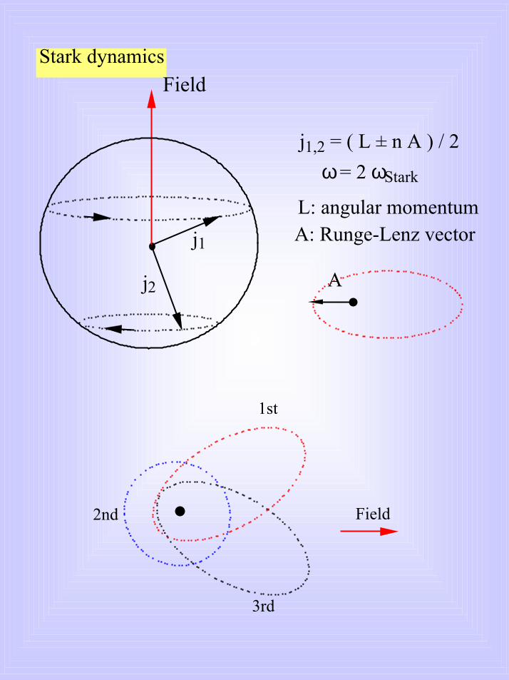
1st

3rd

2nd

Stark dynamics

j1,2 = ( L ± n A ) / 2 ω = 2 ωStark

Field

j1

j2

Field

L: angular momentumA: Runge-Lenz vector

A

Angular momentum wavepacketH(17d) at t=0

Quantum

Classical

t/Torb

/t/Torb

Field

Ener

gy

delay

Probing Stark beats with a short half-cycle pulse

experiment K(388p)

ωorb

ωStark

0 100 200 300 400Delay time (ns)

0.4

0.6

0.8

1.0

Surv

ival

pro

babi

lity

0.5

0.7

0.9ωStark

FDC = 5mV/cm, FHCP= ± 80mV/cm

time

Fiel

d

DC pump

HCP probe

classical simulation

Stark map near n=100 of K(m=0)

350

370

390

410

430

450n=

(-2E)

1/2

0.00 0.01 0.02 0.03 0.04 0.05 0.06 0.07

F0

Diagram of extreme Stark states near n=400

field ionizationthreshold

n=450

n=350

n=399,400,401

FULL MIXINGchaotic spectrum

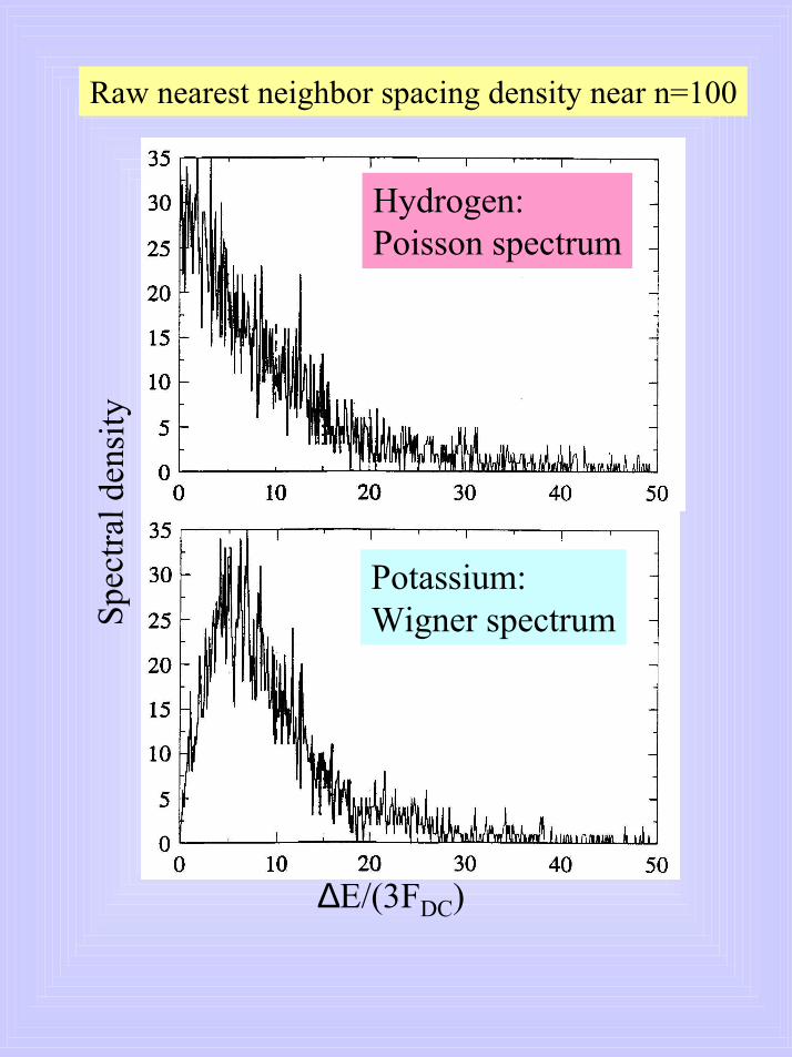
Raw nearest neighbor spacing density near n=100

Hydrogen:Poisson spectrum

Potassium:Wigner spectrumSp

ectr a

l den

s ity

∆E/(3FDC)

0 50 100 150

∆E/(3F DC)

0.00

0.05

0.10

0.15

Spec

tral d

ensi

ty

0.00

0.05

0.10

0.15

0.20

0.25

Step field ==> weighted spectrumweight= overlap with state prior to the step

Potassium

Hydrogen

Coherent states produced by a train of pulses

Fiel

d

time

PUMP

delay time

0 5 10 15 200.20

0.22

0.24

0.26

0.28

0.30

PROBE

100 pulses with scaled frequency ν0

0.25

0.27

0.29

0.31

0.33

0.35

0 5 10 15 20

Surv

ival

pro

babi

lity

Delay time (ns)

ν0=0.7

ν0=0.7

ν0=1.3

ν0=1.3

InitialEnergylevel

p0

q0

Tailoring Rydberg wavefunctions

Classical quantum correspondenceHigh n, large perturbations, short times

Producing and probing coherent states

Recent interesting studies

Information storage and retrieval with Rydberg atomsAhn, Weinacht, and Bucksbaum, Science (2000)

Rydberg antihydrogen production using a fast field stepWesdorp, Robicheaux, Noordam, Phys. Rev. Lett. 84, 3799 (2000

Tp

Torb= 2πn3

Forb= n-4F(t)

Half-cycle pulse (HCP) H(n)

Tp << Torb sudden momentum transfer or ''kick''

�∆p = - dt F(t)

F(t)

F(t) T

The kicked Rydberg atom

ν = 1/TH = Hatom + z F(t)

time

The kicked atom: linear superposition of HCPs

unidirectional

alternating

Ideal testing ground for quantum systems that may become chaotic in their classical limit

Simple driven systems

Experimental realizations

1980s-90s Rydberg atoms + microwave fieldKoch et al (Stony Brook), Bayfield (Pittsburgh)

1994 Atoms in a trap subject to a modulated standing waveRaizen et al (Austin)

1997 Rydberg electrons subject to trains ofhalf-cycle pulsesDunning et al (Rice)

H = Hatom + z F(t)

≈ p2 __ 2

_ 1 __ r

_ Σkz ∆p δ(t-kT)

The 1D periodically kicked atom

p2 __ 2

_ _ ΣkH = 1 __

qq ∆p δ(t-kT)

time dependentLz = Const ==> 2 1/2 degrees of freedom

1 1/2 degrees of freedom

U(kT,0) = Π k

UFree(Hatom,T) U

Kick(∆p)

e-iHatomT eiz∆p

(quantum)

Classical or quantumevolution operator

The 3D periodically kicked atom (unidirectional pulses)

Time evolution ==> simple discrete map

100 δ kicks

1000 δ kicks

finitewidthpulses

experiment

Scaled frequency, ν0 = ν/νorb

3D, n=390, 50 pulses 1D, n=50

Classicalstabilization !!0.6

1.92.1

ν0 = 1.3

3D, n=390

100 101 102 103 104 105 106

Number of pulses, N

10-3

10-2

10-1

100

Surv

ival

pro

babi

lity

0.7

delta kicks

0.1 1 10

0.1

1

How many atoms survive after many pulses ? Experiments and classical simulations

1 100.0

0.1

0.2

0.3

0.4

0.5

0.6

Surv

ival

pro

babi

lity

Isolating stable orbits

Consecutive intersections of a stable orbit with a plane yields a closed loop.

t=k/νp (k=1,2,...)ρ=Const.pρ=Const.

Hatom = + - (ρ2 + z2 )1/2

Lzpz + pρ2 2 2

1

2 2 ρ2 Lz = Const ~ 0

0.0 0.5 1.0 1.5 2.0 2.5 3.0z

-2

-1

0

1

2

p z

Hatom ~ pz

2__ 2

- 1___ | z |

Hatom = -0.5

Hatom = 0

Hatom = -2

Section for ∆p=0, ρ ~ 0, pρ ~ 0, Lz~0

stroboscopic Poincaresection

x

x

Section just before a kick, ρ=0, pρ=0, for ν0=1.3

∆E = ( ∆p )2_____ 2

+ pz ∆p = 0

pz=-∆p/2

Most stable periodic orbit

Fixedpoint

∆p

Correspondence between the 1D and 3D models

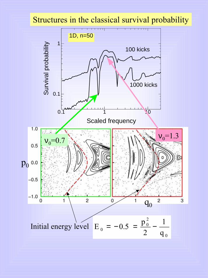
Structures in the classical survival probability

ν0=0.7 ν0=1.3

Initial energy level

p0

q0

0.1

1Su

rviv

al p

roba

bilit

y

0.1 1 10

Scaled frequency

1000 kicks

100 kicks

1D, n=50

0

20

0 q1

2p0.5E −=−=

Classical-quantum correspondence ?

1D kicked atom

∆p

1/q

Classical

Quantum

1D H(n=50) atom after 200 kicks

10-1 100 101Scaled frequency

10-1

100

Surv

ival

pro

babi

lity

1D ==> accurate quantum calculations can be be performed for large n

|Ψ(t)�

|Ψ(0)� = |Φi(t)� : initial state

- Boundary condition

- Dynamics: Schrödinger Equation

- State of the electron:

d|Ψ(t)�dt

i = H |Ψ(t)�

How can we compare classical and quantum dynamics in phase space ?

Husimi distributions:Quantum analog of classical phase space distributions:

Husimi disctributions of Floquet states

Quantum analog of Poincare sections

Usual quantum description of the electron

fw(q,p,t) = dy �q-y|Ψ(t)� �Ψ(t)|q+y� e2ipy

Weyl transform of the density matrix

�

dfwdt = Lqm fw

�1

fw (q,p,t): real quasi probability density (not positive definite)

�A� = dqdp fw(q,p,t) A(q,p)

�|�q|Ψ(t)�|2 = dp fw(q,p,t)

Classical limit: Lqm ≈ Lcl

State of the electron: Wigner function

Dynamics: quantum Liouville equation

π

Alternative quantum description of the electron

minimum uncertainty Gaussian wavepacket

classical

quantum

0.00

0.10

0.15

0.20

0.25

Prob

abili

ty d

ensi

ty

0.05

0.0 0.5 1.0 1.5 2.0 2.5 3.0p

Comparing classical and quantum densities

Husimi distribution: Gaussian smoothed Wigner function

Direct comparison with Wigner functions is difficult

fh (q,p,t) = | �gq,p|Ψ(t)�|2 > 0

gq,p(q') = C e-(q-q')2/a eipq'

Husimi distribution of the 1D n=50 level

__p02

2-0.5 = _ 1 __

q0

PCL ~ (p0)-1/2

probability maximizesat the outer turning point

classical

PQM(q,p)

q0

p0

0.00.5

1.01.5

2.02.5

-2

-1

0

1

2-0.05

-0.03

-0.01

0.01

0.03

0.05

Classical phase space vs quantum Husimi distributions

outgoing flux(norm not conserved)finite Hilbert

space

complex quasi eigenenergy period-oneevolution operator

Floquet analysis in a finite basis set

Floquet states:

Soft boudary conditions

U(T,0) |φk� = e-iεkT |φk�

Σ|Ψ(NT)� = ck e-iεkNT |φk�

k

Stable Floquet states: Im(εk) = 0

Husimi distributions of stable Floquet states for ν0=1.3

quantum

quantum

classical

Periodic orbits and fixed points

stable unstable

Any trace of unstable periodic orbits in quantum mechanics ?

∆p

Quantum localization for high frequencies

n=50, ν0=16.8, ∆p

0=-0.3

0.4

0.5

0.6

0.7

0.8

0.9

1.0

Surv

ival

pro

babi

lity

1 10 100Number of kicks

classical

quantum

breaktime

-2.5-1.5

-0.50.5

1.5

2.5

0.00.5

1.0

1.5

2.0

Husimi distribution of a stable Floquet state for ν0=16.8

q0p0

Stable Floquet states ==> scarred statesHeller (1980s)

unstable periodic orbit

P(q,p)

Why does the survival probability oscillate ?

E=0

Localization in the continuum

Classical phase space

Initiallevel

�

Husimi distributions of stable Floquet states

X: classical fixed points : Unstable periodic orbits

Correspondence for high frequencies, ν0=16.8and strong perturbations, ∆p0=-0.3

Classical phase space

Initiallevel

�

Husimi distributions of stable Floquet states

X: classical fixed points

Lack of correspondence for weak perturbations, ∆p0=+0.01

n=50ν0=16.8

What do periodic orbits resemble ?

t)mcos(2π2FFkT)-δ(t ∆pF(t)1m

avavk

ν��≥

+==

t)mcos(2π2qFHH(t)1m

avStark ν�≥

−=

avatomStark qFHH −=

Fav=∆p/T = average field

Stark orbit

Coulomborbit

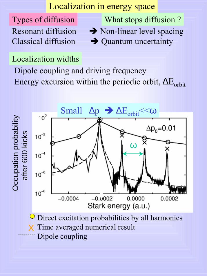
Localization in energy space

Direct excitation probabilities by all harmonicsTime averaged numerical resultDipole coupling

X

Occ

upat

ion

prob

abilit

yaf

ter 6

00 k

icks

Types of diffusionResonant diffusion � Non-linear level spacingClassical diffusion � Quantum uncertainty

Localization widths

What stops diffusion ?

Dipole coupling and driving frequencyEnergy excursion within the periodic orbit, ∆Eorbit

ω

Small ∆p � ∆Eorbit<<ω

Correspondence for the localization widthO

ccup

atio

n pr

obab

ility

afte

r 600

kic

ks ω

Large ∆p � ∆Eorbit> ω

Direct excitation probabilities by all harmonicsDipole coupling

∆Eorbit

The kicked Rydberg atom

Long timesClassical quantumCorrespondence

- short times- high n- large perturbations

Classical

quantum

Outlook

- Localization in 3D- Adding noise and other trains of pulses- Any train of pulses leading to long lived coherent states ?

Cross-disciplinary

Transport of atoms through solids

i

dissipative interactionwith the environment

= [Hatom,ρ] + R ρdρdt

+ V(r)p2

2Hatom =Screened ion field

STATE OF THE SYSTEM: ρcl(r,p,t)DYNAMICS: classical Liouville equation

STATE OF THE SYSTEM: reduced density matrix ρ(t)

DYNAMICS: quantum Liouville equation

CLASSICAL TRANSPORT:

Transmission of fast atoms through solids The randomlykicked atom

Microscopic interaction

Vint

)p(∆V~ i|e|f pd∆dtdP

intr.pi∆ ��

��

�∝

First order transition probability per unit time

Fourier transform: Probability distribution of kicks

Transition amplitudefor a given ∆p

Similarity to quantum optics

Microscopic approach: Langevin equation

kΣr .

1N Σ

N.u=1

ρ(t) = |Ψu(t)��Ψu(t)|quantum trajectory

Random multiple elastic and inelasticcollisions with particles in the solid.

H = Hatom ∆pk δ(t-tk)

Langevin equation: undeterministic Schrödinger equation