Parties, Models, Mobsters: A New Implementation of Model ... · Parties, Models, Mobsters: A New Implementation of Model-Based Recursive Partitioning in R Achim Zeileis Universit¨at

Parties, Models, Mobsters: A New Implementation

of Model-Based Recursive Partitioning in R

Achim Zeileis

Universitat InnsbruckTorsten Hothorn

Universitat Zurich

Abstract

MOB is a generic algorithm for model-based recursive partitioning (Zeileis, Hothorn,and Hornik 2008). Rather than fitting one global model to a dataset, it estimates localmodels on subsets of data that are “learned”by recursively partitioning. It proceeds in thefollowing way: (1) fit a parametric model to a data set, (2) test for parameter instabilityover a set of partitioning variables, (3) if there is some overall parameter instability, splitthe model with respect to the variable associated with the highest instability, (4) repeatthe procedure in each of the resulting subsamples. It is discussed how these steps of theconceptual algorithm are translated into computational tools in an object-oriented man-ner, allowing the user to plug in various types of parametric models. For representing theresulting trees, the R package partykit is employed and extended with generic infrastruc-ture for recursive partitions where nodes are associated with statistical models. Comparedto the previously available implementation in the party package, the new implementationsupports more inference options, is easier to extend to new models, and provides moreconvenience features.

Keywords: parametric models, object-orientation, recursive partitioning.

1. Overview

To implement the model-based recursive partitioning (MOB) algorithm of Zeileis et al. (2008)in software, infrastructure for three aspects is required: (1) statistical “models”, (2) recursive“party”tions, and (3) “mobsters” carrying out the MOB algorithm.

Along with Zeileis et al. (2008), an implementation of all three steps was provided in theparty package (Hothorn, Hornik, Strobl, and Zeileis 2015) for the R system for statisticalcomputing (R Core Team 2013). This provided one very flexible mob() function combiningparty’s S4 classes for representing trees with binary splits and the S4 model wrapper functionsfrom modeltools (Hothorn, Leisch, and Zeileis 2013). However, while this supported manyapplications of interest, it was somewhat limited in several directions: (1) The S4 wrappers forthe models were somewhat cumbersome to set up. (2) The tree infrastructure was originallydesigned for ctree() and somewhat too narrowly focused on it. (3) Writing new “mobster”interfaces was not easy because of using unexported S4 classes.

Hence, a leaner and more flexible interface (based on S3 classes) is now provided in partykit

(Hothorn and Zeileis 2015): (1) New models are much easier to provide in a basic version andcustomization does not require setting up an additional S4 class-and-methods layer anymore.(2) The trees are built on top of partykit’s flexible ‘party’ objects, inheriting many useful

2 Model-Based Recursive Partitioning in R

methods and providing new ones dealing with the fitted models associated with the tree’snodes. (3) New “mobsters” dedicated to specific models, e.g., lmtree() and glmtree() forMOBs of (generalized) linear models, are readily provided.

The remainder of this vignette is organized as follows: Section 2 very briefly reviews theoriginal MOB algorithm of Zeileis et al. (2008) and also highlights relevant subsequent work.Section 3 introduces the new mob() function in partykit in detail, discussing how all stepsof the MOB algorithm are implemented and which options for customization are available.For illustration logistic-regression-based recursive partitioning is applied to the Pima Indiansdiabetes data set from the UCI machine learning repository (Bache and Lichman 2013).Section 4 and 5 present further illustrative examples (including replications from Zeileis et al.2008) before Section 6 provides some concluding remarks.

2. MOB: Model-based recursive partitioning

First, the theory underling the MOB (model-based recursive partitioning) is briefly reviewed;a more detailed discussion is provided by Zeileis et al. (2008). To fix notation, consider aparametric model M(Y, θ) with (possibly vector-valued) observations Y and a k-dimensionalvector of parameters θ. This model could be a (possibly multivariate) normal distribution forY , a psychometric model for a matrix of responses Y , or some kind of regression model whenY = (y, x) can be split up into a dependent variable y and regressors x. An example for thelatter could be a linear regression model y = x⊤θ or a generalized linear model (GLM) or asurvival regression.

Given n observations Yi (i = 1, . . . , n) the model can be fitted by minimizing some objectivefunction

∑ni=1

Ψ(Yi, θ), e.g., a residual sum of squares or a negative log-likelihood leading toordinary least squares (OLS) or maximum likelihood (ML) estimation, respectively.

If a global model for all n observations does not fit well and further covariates Z1, . . . , Zℓ areavailable, it might be possible to partition the n observations with respect to these variablesand find a fitting local model in each cell of the partition. The MOB algorithm tries tofind such a partition adaptively using a greedy forward search. The reasons for lookingat such local models might be different for different types of models: First, the detectionof interactions and nonlinearities in regression relationships might be of interest just like instandard classification and regression trees (see e.g., Zeileis et al. 2008). Additionally, however,this approach allows to add explanatory variables to models that otherwise do not haveregressors or where the link between the regressors and the parameters of the model is inclear(this idea is pursued by Strobl, Wickelmaier, and Zeileis 2011). Finally, the model-based treecan be employed as a thorough diagnostic test of the parameter stability assumption (alsotermed measurement invariance in psychometrics). If the tree does not split at all, parameterstability (or measurement invariance) cannot be rejected while a tree with splits would indicatein which way the assumption is violated (Strobl, Kopf, and Zeileis 2015, employ this idea inpsychometric item response theory models).

The basic idea is to grow a tee in which every node is associated with a model of type M. Toassess whether splitting of the node is necessary a fluctuation test for parameter instability isperformed. If there is significant instability with respect to any of the partitioning variablesZj , the node is splitted into B locally optimal segments (the currenct version of the softwarehas B = 2 as the default and as the only option for numeric/ordered variables) and then the

Achim Zeileis, Torsten Hothorn 3

procedure is repeated in each of the B children. If no more significant instabilities can befound, the recursion stops. More precisely, the steps of the algorithm are

1. Fit the model once to all observations in the current node.

2. Assess whether the parameter estimates are stable with respect to every partitioningvariable Z1, . . . , Zℓ. If there is some overall instability, select the variable Zj associatedwith the highest parameter instability, otherwise stop.

3. Compute the split point(s) that locally optimize the objective function Ψ.

4. Split the node into child nodes and repeat the procedure until some stopping criterionis met.

This conceptual framework is extremely flexible and allows to adapt it to various tasks bychoosing particular models, tests, and methods in each of the steps:

1. Model estimation: The original MOB introduction (Zeileis et al. 2008) discussed re-gression models: OLS regression, GLMs, and survival regression. Subsequently, Grun,Kosmidis, and Zeileis (2012) have also adapted MOB to beta regression for limited re-sponse variables. Furthermore, MOB provides a generic way of adding covariates tomodels that otherwise have no regressors: this can either serve as a check whether themodel is indeed independent from regressors or leads to local models for subsets. Bothviews are of interest when employing MOB to detect parameter instabilities in psycho-metric models for item responses such as the Bradley-Terry or the Rasch model (seeStrobl et al. 2011, 2015, respectively).

2. Parameter instability tests: To assess the stability of all model parameters across acertain partitioning variable, the general class of score-based fluctuation tests proposedby Zeileis and Hornik (2007) is employed. Based on the empirical score function obser-vations (i.e., empirical estimating functions or contributions to the gradient), orderedwith respect to the partitioning variable, the fluctuation or instability in the model’s pa-rameters can be tested. From this general framework the Andrews’ supLM test is usedfor assessing numerical partitioning variables and a χ2 test for categorical partitioningvariables (see Zeileis 2005 and Merkle and Zeileis 2013 for unifying views emphasizingregression and psychometric models, respectively). Furthermore, the test statistics forordinal partitioning variables suggested by Merkle, Fan, and Zeileis (2014) have beenadded as further options (but are not used by default as the simulation of p-values iscomputationally demanding).

3. Partitioning: As the objective function Ψ is additive, it is easy to compute a singleoptimal split point (or cut point or break point). For each conceivable split, the model isestimated on the two resulting subsets and the resulting objective functions are summed.The split that optimizes this segmented objective function is then selected as the optimalsplit. For optimally splitting the data into B > 2 segments, the same idea can be usedand a full grid search can be avoided by employing a dynamic programming algorithms(Hawkins 2001; Bai and Perron 2003) but at the moment the latter is not implementedin the software. Optionally, however, categorical partitioning variables can be split intoall of their categories (i.e., in that case B is set to the number of levels without searchingfor optimal groupings).


4. Pruning: For determining the optimal size of the tree, one can either use a pre-pruningor post-pruning strategy. For the former, the algorithm stops when no significant pa-rameter instabilities are detected in the current node (or when the node becomes toosmall). For the latter, one would first grow a large tree (subject only to a minimalnode size requirement) and then prune back splits that did not improve the model, e.g.,judging by information criteria such as AIC or BIC (see e.g., Su, Wang, and Fan 2004).Currently, pre-pruning is used by default (via Bonferroni-corrected p-values from thescore-based fluctuation tests) but AIC/BIC-based post-pruning is optionally available(especially for large data sets where traditional significance levels are not useful).

In the following it is discussed how most of the options above are embedded in a commoncomputational framework using R’s facilities for model estimation and object orientation.

3. A new implementation in R

This section introduces a new implementation of the general model-based recursive partition-ing (MOB) algorithm in R. Along with Zeileis et al. (2008), a function mob() had been intro-duced to the party package (Hothorn et al. 2015) which continues to work but it turned outto be somewhat unflexible for certain applications/extensions. Hence, the partykit package(Hothorn and Zeileis 2015) provides a completely rewritten (and not backward compatible)implementation of a new mob() function along with convenience interfaces lmtree() andglmtree() for fitting linear model and generalized linear model trees, respectively. The func-tion mob() itself is intended to be the workhorse function that can also be employed to quicklyexplore new models – whereas lmtree() and glmtree() will be the typical user interfacesfacilitating applications.

The new mob() function has the following arguments:

mob(formula, data, subset, na.action, weights, offset,

fit, control = mob_control(), ...)

All arguments in the first line are standard for modeling functions in R with a formula

interface. They are employed by mob() to do some data preprocessing (described in detailin Section 3.1) before the fit function is used for parameter estimation on the preprocesseddata. The fit function has to be set up in a certain way (described in detail in Section 3.2)so that mob() can extract all information that is needed in the MOB algorithm for parameterinstability tests (see Section 3.3) and partitioning/splitting (see Section 3.4), i.e., the estimatedparameters, the associated objective function, and the score function contributions. A list ofcontrol options can be set up by the mob_control() function, including options for pruning(see Section 3.5). Additional arguments ... are passed on to the fit function.

The result is an object of class ‘modelparty’ inheriting from ‘party’. The info element ofthe overall ‘party’ and the individual ‘node’s contain various informations about the models.Details are provided in Section 3.6.

Finally, a wide range of standard (and some extra) methods are available for working with‘modelparty’ objects, e.g., for extracting information about the models, for visualization,computing predictions, etc. The standard set of methods is introduced in Section 3.7. How-ever, as will be discussed there, it may take some effort by the user to efficiently compute


certain pieces of information. Hence, convenience interfaces such as lmtree() or glmtree()can alleviate these obstacles considerably, as illustrated in Section 3.8.

3.1. Formula processing and data preparation

The formula processing within mob() is essentially done in “the usual way”, i.e., there is aformula and data and optionally further arguments such as subset, na.action, weights,and offset. These are processed into a model.frame from which the response and thecovariates can be extracted and passed on to the actual fit function.

As there are possibly three groups of variables (response, regressors, and partitioning vari-ables), the Formula package (Zeileis and Croissant 2010) is employed for processing thesethree parts. Thus, the formula can be of type y ~ x1 + ... + xk | z1 + ... + zl wherethe variables on the left of the | specify the data Y and the variables on the right specifythe partitioning variables Zj . As pointed out above, the Y can often be split up into re-sponse (y in the example above) and regressors (x1, . . . , xk in the example above). If thereare no regressors and just constant fits are employed, then the formula can be specified asy ~ 1 | z1 + ... + zl.

So far, this formula representation is really just a specification of groups of variables and doesnot imply anything about the type of model that is to be fitted to the data in the nodes of thetree. The mob() function does not know anything about the type of model and just passes(subsets of) the y and x variables on to the fit function. Only the partitioning variables zare used internally for the parameter instability tests (see Section 3.3).

As different fit functions will require the data in different formats, mob_control() allows toset the ytype and xtype. The default is to assume that y is just a single column of the modelframe that is extracted as a ytype = "vector". Alternatively, it can be a "data.frame" ofall response variables or a "matrix" set up via model.matrix(). The options "data.frame"and "matrix" are also available for xtype with the latter being the default. Note that if"matrix" is used, then transformations (e.g., logs, square roots etc.) and dummy/interactioncodings are computed and turned into columns of a numeric matrix while for "data.frame"the original variables are preserved.

By specifying the ytype and xtype, mob() is also provided with the information on how tocorrectly subset y and x when recursively partitioning data. In each step, only the subset ofy and x pertaining to the current node of the tree is passed on to the fit function. Similarly,subsets of weights and offset are passed on (if specified).

Illustration

For illustration, we employ the popular benchmark data set on diabetes among Pima Indianwomen that is provided by the UCI machine learning repository (Bache and Lichman 2013)and available in the mlbench package (Leisch and Dimitriadou 2012):

R> data("PimaIndiansDiabetes", package = "mlbench")

Following Zeileis et al. (2008) we want to fit a model for diabetes employing the plasmaglucose concentration glucose as a regressor. As the influence of the remaining variables ondiabetes is less clear, their relationship should be learned by recursive partitioning. Thus,we employ the following formula:


R> pid_formula <- diabetes ~ glucose | pregnant + pressure + triceps +

+ insulin + mass + pedigree + age

Before passing this to mob(), a fit function is needed and a logistic regression function is setup in the following section.

3.2. Model fitting and parameter estimation

The mob() function itself does not actually carry out any parameter estimation by itself,but assumes that one of the many R functions available for model estimation is supplied.However, to be able to carry out the steps of the MOB algorithm, mob() needs to able toextract certain pieces of information: especially the estimated parameters, the correspondingobjective function, and associated score function contributions. Also, the interface of thefitting function clearly needs to be standardized so that mob() knows how to invoke themodel estimation.

Currently, two possible interfaces for the fit function can be employed:

1. The fit function can take the following inputs

fit(y, x = NULL, start = NULL, weights = NULL, offset = NULL, ...,

estfun = FALSE, object = FALSE)

where y, x, weights, offset are (the subset of) the preprocessed data. In start startingvalues for the parameter estimates may be supplied and ... is passed on from the mob()function. The fit function then has to return an output list with the following elements:

❼ coefficients: Estimated parameters θ.

❼ objfun: Value of the minimized objective function∑

iΨ(yi, x,θ).

❼ estfun: Empirical estimating functions (or score function contributions) Ψ′(yi, xi, θ).Only needed if estfun = TRUE, otherwise optionally NULL.

❼ object: A model object for which further methods could be available (e.g., predict(),or fitted(), etc.). Only needed if object = TRUE, otherwise optionally NULL.

By making estfun and object optional, the fitting function might be able to savecomputation time by only optimizing the objective function but avoiding further com-putations (such as setting up covariance matrix, residuals, diagnostics, etc.).

2. The fit function can also of a simpler interface with only the following inputs:

fit(y, x = NULL, start = NULL, weights = NULL, offset = NULL, ...)

The meaning of all arguments is the same as above. However, in this case fit needs toreturn a classed model object for which methods to coef(), logLik(), and estfun()

(see Zeileis 2006, and the sandwich package) are available for extracting the parameterestimates, the maximized log-likelihood, and associated empirical estimating functions(or score contributions), respectively. Internally, a function of type (1) is set up bymob() in case a function of type (2) is supplied. However, as pointed out above, afunction of type (1) might be useful to save computation time.


In either case the fit function can, of course, choose to ignore any arguments that are notapplicable, e.g., if the are no regressors x in the model or if starting values or not supported.

The fit function of type (2) is typically convenient to quickly try out a new type of modelin recursive partitioning. However, when writing a new mob() interface such as lmtree()

or glmtree(), it will typically be better to use type (1). Similarly, employing supportingstarting values in fit is then recommended to save computation time.

Illustration

For recursively partitioning the diabetes ~ glucose relationship (as already set up in theprevious section), we employ a logistic regression model. An interface of type (2) can be easilyset up:

R> logit <- function(y, x, start = NULL, weights = NULL, offset = NULL, ...) {

+ glm(y ~ 0 + x, family = binomial, start = start, ...)

+ }

Thus, y, x, and the starting values are passed on to glm() which returns an object of class‘glm’ for which all required methods (coef(), logLik(), and estfun()) are available.

Using this fit function and the formula already set up above the MOB algorithm can beeasily applied to the PimaIndiansDiabetes data:

R> pid_tree <- mob(pid_formula, data = PimaIndiansDiabetes, fit = logit)

The result is a logistic regression tree with three terminal nodes that can be easily visualizedvia plot(pid_tree) (see Figure 1) and printed:

R> pid_tree

Model-based recursive partitioning (logit)

Model formula:

diabetes ~ glucose | pregnant + pressure + triceps + insulin +

mass + pedigree + age

Fitted party:

[1] root

| [2] mass <= 26.3: n = 167

| x(Intercept) xglucose

| -9.95151 0.05871

| [3] mass > 26.3

| | [4] age <= 30: n = 304

| | x(Intercept) xglucose

| | -6.70559 0.04684

| | [5] age > 30: n = 297

| | x(Intercept) xglucose

| | -2.77095 0.02354


Number of inner nodes: 2

Number of terminal nodes: 3

Number of parameters per node: 2

Objective function: 355.5

The tree finds three groups of Pima Indian women:

#2 Women with low body mass index that have on average a low risk of diabetes, howeverthis increases clearly with glucose level.

#4 Women with average and high body mass index, younger than 30 years, that have ahigher avarage risk that also increases with glucose level.

#5 Women with average and high body mass index, older than 30 years, that have a highavarage risk that increases only slowly with glucose level.

Note that the example above is used for illustration here and glmtree() is recommended overusing mob() plus manually setting up a logit() function. The same tree structure can befound via:

R> pid_tree2 <- glmtree(diabetes ~ glucose | pregnant +

+ pressure + triceps + insulin + mass + pedigree + age,

+ data = PimaIndiansDiabetes, family = binomial)

However, glmtree() is slightly faster as it avoids many unnecessary computations, see Sec-tion 3.8 for further details.

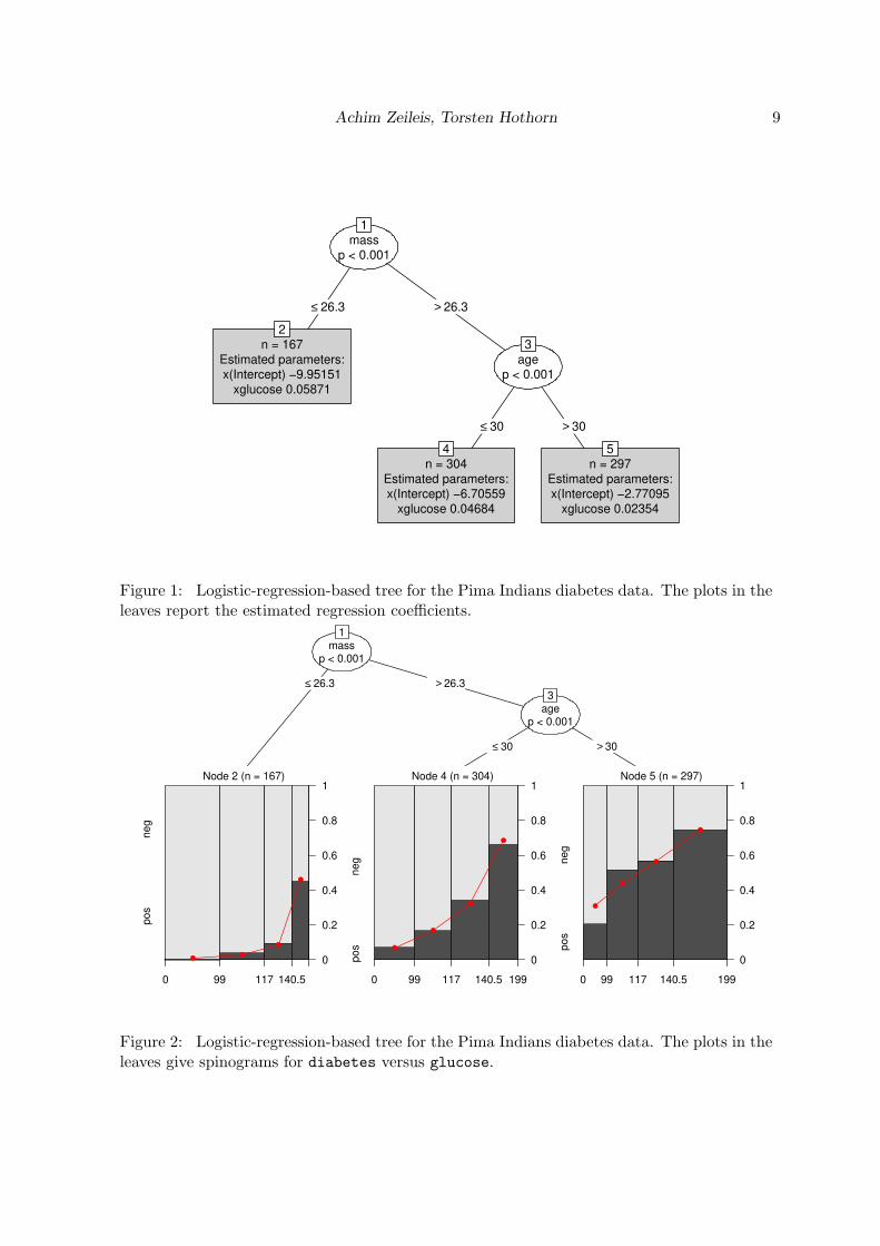
Here, we only point out that plot(pid_tree2) produces a nicer visualization (see Figure 2).As y is diabetes, a binary variable, and x is glucose, a numeric variable, a spinogram ischosen automatically for visualization (using the vcd package, Meyer, Zeileis, and Hornik2006). The x-axis breaks in the spinogram are the five-point summary of glucose on the fulldata set. The fitted lines are the mean predicted probabilities in each group.

3.3. Testing for parameter instability

In each node of the tree, first the parametric model is fitted to all observations in that node(see Section 3.2). Subsequently it is of interest to find out whether the model parametersare stable over each particular ordering implied by the partitioning variables Zj or whethersplitting the sample with respect to one of the Zj might capture instabilities in the parametersand thus improve the fit. The tests used in this step belong to the class of generalized M-fluctuation tests (Zeileis 2005; Zeileis and Hornik 2007). Depending on the class of each ofthe partitioning variables in z different types of tests are chosen by mob():

1. For numeric partitioning variables (of class ‘numeric’ or ‘integer’) the supLM statisticis used which is the maximum over all single-split LM statistics. Associated p-valuescan be obtained from a table of critical values (based on Hansen 1997) stored withinthe package.


mass

p < 0.001

1

≤ 26.3 > 26.3

n = 167

Estimated parameters:

x(Intercept) −9.95151

xglucose 0.05871

2

age

p < 0.001

3

≤ 30 > 30

n = 304



xglucose 0.04684

4

n = 297



xglucose 0.02354

5

Figure 1: Logistic-regression-based tree for the Pima Indians diabetes data. The plots in theleaves report the estimated regression coefficients.

mass

p < 0.001

1

≤ 26.3 > 26.3

Node 2 (n = 167)

0 99 117 140.5

pos

neg

0

0.2

0.4

0.6

0.8

1

●●

●

●

age

p < 0.001

3

≤ 30 > 30

Node 4 (n = 304)

0 99 117 140.5 199

pos

neg

0

0.2

0.4

0.6

0.8

1

●

●

●

●

Node 5 (n = 297)

0 99 117 140.5 199

pos

neg

0

0.2

0.4

0.6

0.8

1

●

●

●

●

Figure 2: Logistic-regression-based tree for the Pima Indians diabetes data. The plots in theleaves give spinograms for diabetes versus glucose.


If there are ties in the partitioning variable, the sequence of LM statistics (and hencetheir maximum) is not unique and hence the results by default may depend to somedegree on the ordering of the observations. To explore this, the option breakties =

TRUE can be set in mob_control() which breaks ties randomly. If there are are onlyfew ties, the influence is often negligible. If there are many ties (say only a dozenunique values of the partitioning variable), then the variable may be better treated asan ordered factor (see below).

2. For categorical partitioning variables (of class ‘factor’), a χ2 statistic is employed whichcaptures the fluctuation within each of the categories of the partitioning variable. Thisis also an LM -type test and is asymptotically equivalent to the corresponding likelihoodratio test. However, it is somewhat cheaper to compute the LM statistic because themodel just has to be fitted once in the current node and not separately for each categoryof each possible partitioning variable. See also Merkle et al. (2014) for a more detaileddiscussion.

3. For ordinal partitioning variables (of class ‘ordered’ inheriting from ‘factor’) the sameχ2 as for the unordered categorical variables is used by default (as suggested by Zeileiset al. 2008). Although this test is consistent for any parameter instabilities acrossordered variables, it does not exploit the ordering information.

Recently, Merkle et al. (2014) proposed an adapted maxLM test for ordered variablesand, alternatively, a weighted double maximum test. Both are optionally availble inthe new mob() implementation by setting ordinal = "L2" or ordinal = "max" inmob_control(), respectively. Unfortunately, computing p-values from both tests ismore costly than for the default ordinal = "chisq". For "L2" suitable tables of criticalvalues have to be simulated on the fly using ordL2BB() from the strucchange package(Zeileis, Leisch, Hornik, and Kleiber 2002). For "max" a multivariate normal probabilityhas to be computed using the mvtnorm package (Genz et al. 2015).

All of the parameter instability tests above can be computed in an object-oriented manner asthe “estfun” has to be available for the fitted model object. (Either by computing it in thefit function directly or by providing a estfun() extractor, see Section 3.2.)

All tests also require an estimate of the corresponding variance-covariance matrix of theestimating functions. The default is to compute this using an outer-product-of-gradients(OPG) estimator. Alternatively, the corrsponding information matrix or sandwich matrixcan be used if: (a) the estimating functions are actually maximum likelihood scores, and(b) a vcov() method (based on an estimate of the information) is provided for the fittedmodel objects. The corresponding option in mob_control() is to set vcov = "info" or vcov= "sandwich" rather than vcov = "opg" (the default).

For each of the j = 1, . . . , ℓ partitioning variables in z the test selected in the control optionsis employed and the corresponding p-value pj is computed. To adjust for multiple testing,the p values can be Bonferroni adjusted (which is the default). To determine whether thereis some overall instability, it is checked whether the minial p-value pj∗ = minj=1,...,ℓ pj fallsbelow a pre-specified significance level α (by default α = 0.05) or not. If there is significantinstability, the variable Zj∗ associated with the minimal p-value is used for splitting the node.


Illustration

In the logistic-regression-based MOB pid_tree computed above, the parameter instabil-ity tests can be extracted using the sctest() function from the strucchange package (forstructural change test). In the first node, the test statistics and Bonferroni-corrected p-valuesare:

R> library("strucchange")

R> sctest(pid_tree, node = 1)

pregnant pressure triceps insulin mass pedigree

statistic 2.989e+01 7.5024 15.94095 6.5969 4.881e+01 18.33476

p.value 9.778e-05 0.9104 0.06474 0.9701 8.317e-09 0.02253

age

statistic 4.351e+01

p.value 1.183e-07

Thus, the body mass index has the lowest p-value and is highly significant and hence used forsplitting the data. In the second node, no further significant parameter instabilities can bedetected and hence partitioning stops in that branch.


pregnant pressure triceps insulin mass pedigree age

statistic 10.3923 4.3538 5.9114 3.786 10.4749 3.626 6.0978

p.value 0.4903 0.9998 0.9869 1.000 0.4785 1.000 0.9818

In the third node, however, there is still significant instability associated with the age variableand hence partitioning continues.



statistic 2.674e+01 6.1758 7.3468 7.896 9.1546 17.96439

p.value 4.434e-04 0.9845 0.9226 0.870 0.7033 0.02647

age

statistic 3.498e+01

p.value 8.099e-06

Because no further instabilities can be found in the fourth and fifth node, the recursivepartitioning stops there.

3.4. Splitting

In this step, the observations in the current node are split with respect to the chosen parti-tioning variable Zj∗ into B child nodes. As pointed out above, the mob() function currentlyonly supports binary splits, i.e., B = 2. For deterimining the split point, an exhaustive search


procedure is adopted: For each conceivable split point in Zj∗ , the two subset models are fitand the split associated with the minimal value of the objective function Ψ is chosen.

Computationally, this means that the fit function is applied to the subsets of y and x foreach possibly binary split. The “objfun” values are simply summed up (because the objectivefunction is assumed to be additive) and its minimum across splits is determined. In a searchover a numeric partitioning variable, this means that typically a lot of subset models have tobe fitted and often these will not vary a lot from one split to the next. Hence, the parameterestimates“coefficients” from the previous split are employed as start values for estimatingthe coefficients associated with the next split. Thus, if the fit function makes use of thesestarting values, the model fitting can often be speeded up.

Illustration

For the Pima Indians diabetes data, the split points found for pid_tree are displayed bothin the print output and the visualization (see Figure 1 and 2).

3.5. Pruning

By default, the size of mob() trees is determined only by the significance tests, i.e., whenthere is no more significant parameter instability (by default at level α = 0.05) the treestops growing. Additional stopping criteria are only the minimal node size (minsize) and themaximum tree depth (maxdepth, by default infinity).

However, for very large sample size traditional significance levels are typically not usefulbecause even tiny parameter instabilities can be detected. To avoid overfitting in such asituation, one would either have to use much smaller significance levels or add some formof post-pruning to reduce the size of the tree afterwards. Similarly, one could wish to firstgrow a very large tree (using a large α level) and then prune it afterwards, e.g., using someinformation criterion like AIC or BIC.

To accomodate such post-pruning strategies, mob_control() has an argument prune thatcan be a function(objfun, df, nobs) that either returns TRUE if a node should be prunedor FALSE if not. The arguments supplied are a vector of objective function values in thecurrent node and the sum of all child nodes, a vector of corresponding degrees of freedom,and the number of observations in the current node and in total. For example if the objectivefunction used is the negative log-likelihood, then for BIC-based pruning the prune func-tion is: (2 * objfun[1] + log(nobs[1]) * df[1]) < (2 * objfun[2] + log(nobs[2])

* df[2]). As the negative log-likelihood is the default objective function when using the“simple” fit interface, prune can also be set to "AIC" or "BIC" and then suitable functionswill be set up internally. Note, however, that for other objective functions this strategy is notappropriate and the functions would have to be defined differently (which lmtree() does forexample).

In the literature, there is no clear consensus as to how many degrees of freedom should beassigned to the selection of a split point. Hence, mob_control() allows to set dfsplit whichby default is dfsplit = TRUE and then as.integer(dfsplit) (i.e., 1 by default) degreesof freedom per split are used. This can be modified to dfsplit = FALSE (or equivalentlydfsplit = 0) or dfsplit = 3 etc. for lower or higher penalization of additional splits.


Illustration

With n = 768 observations, the sample size is quite reasonable for using the classical signifi-cance level of α = 0.05 which is also reflected by the moderate tree size with three terminalnodes. However, if we wished to explore further splits, a conceivable strategy could be thefollowing:

R> pid_tree3 <- mob(pid_formula, data = PimaIndiansDiabetes,

+ fit = logit, control = mob_control(verbose = TRUE,

+ minsize = 50, maxdepth = 4, alpha = 0.9, prune = "BIC"))

This first grows a large tree until the nodes become too small (minimum node size: 50 ob-servations) or the tree becomes too deep (maximum depth 4 levels) or the significance levelscome very close to one (larger than α = 0.9). Here, this large tree has eleven nodes whichare subsequently pruned based on whether or not they improve the BIC of the model. Forthis data set, the resulting BIC-pruned tree is in fact identical to the pre-pruned pid_tree

considered above.

3.6. Fitted ‘party’ objects

The result of mob() is an object of class ‘modelparty’ inheriting from ‘party’. See the othervignettes in the partykit package (Hothorn and Zeileis 2015) for more details of the general‘party’ class. Here, we just point out that the main difference between a ‘modelparty’ anda plain ‘party’ is that additional information about the data and the associated models isstored in the info elements: both of the overall ‘party’ and the individual ‘node’s. Thedetails are exemplified below.

Illustration

In the info of the overall ‘party’ the following information is stored for pid_tree:

R> names(pid_tree$info)

[1] "call" "formula" "Formula" "terms" "fit" "control"

[7] "dots" "nreg"

The call contains the mob() call. The formula and Formula are virtually the same but aresimply stored as plain ‘formula’ and extended ‘Formula’ (Zeileis and Croissant 2010) objects,respectively. The terms contain separate lists of terms for the response (and regressor)and the partitioning variables. The fit, control and dots are the arguments that wereprovided to mob() and nreg is the number of regressor variables.

Furthermore, each node of the tree contains the following information:

R> names(pid_tree$node$info)

[1] "criterion" "p.value" "coefficients" "objfun"

[5] "object" "converged" "nobs"


The coefficients, objfun, and object are the results of the fit function for that node.In nobs and p.value the number of observations and the minimal p-value are provided,respectively. Finally, test contains the parameter instability test results. Note that theobject element can also be suppressed through mob_control() to save memory space.

3.7. Methods

There is a wide range of standard methods available for objects of class ‘modelparty’. Thestandard print(), plot(), and predict() build on the corresponding methods for ‘party’objects but provide some more special options. Furthermore, methods are provided thatare typically available for models with formula interfaces: formula() (optionally one canset extended = TRUE to get the ‘Formula’), getCall(), model.frame(), weights(). Fi-nally, there is a standard set of methods for statistical model objects: coef(), residuals(),logLik() (optionally setting dfsplit = FALSE suppresses counting the splits in the degreesof freedom, see Section 3.5), deviance(), fitted(), and summary().

Some of these methods rely on reusing the corresponding methods for the individual modelobjects in the terminal nodes. Functions such as coef(), print(), summary() also take anode argument that can specify the node IDs to be queried.

Two methods have non-standard arguments to allow for additional flexibility when dealingwith model trees. Typically, “normal” users do not have to use these arguments directly butthey are very flexible and facilitate writing convenience interfaces such as glmtree() (seeSection 3.8).

❼ The predict() method has the following arguments: predict(object, newdata =

NULL, type = "node", ...). The argument type can either be a function or a char-acter string. More precisely, if type is a function it should be a function (object,

newdata = NULL, ...) that returns a vector or matrix of predictions from a fittedmodel object either with or without newdata. If type is a character string, such afunction is set up internally as predict(object, newdata = newdata, type = type,

...), i.e., it relies on a suitable predict() method being available for the fitted modelsassociated with the ‘party’ object.

❼ The plot() method has the following arguments: plot(x, terminal_panel = NULL,

FUN = NULL). This simply calls the plot() method for ‘party’ objects with a custompanel function for the terminal panels. By default, node_terminal is used to includesome short text in each terminal node. This text can be set up by FUN with the defaultbeing the number of observations and estimated parameters. However, more elaborateterminal panel functions can be written, as done for the convenience interfaces.

Finally, two S3-style functions are provided without the corresponding generics (as thesereside in packages that partykit does not depend on). The sctest.modelparty can be usedin combination with the sctest() generic from strucchange as illustrated in Section 3.3. Therefit.modelparty function extracts (or refits if necessary) the fitted model objects in thespecified nodes (by default from all nodes).

Illustration

The plot() and print() methods have already been illustrated for the pid_tree above.


However, here we add that the print() method can also be used to show more detailedinformation about particular nodes instead of showing the full tree:

R> print(pid_tree, node = 3)


-- Node 3 --


x(Intercept) xglucose

-4.61015 0.03426

Objective function:

344.2

Parameter instability tests:


statistic 2.674e+01 6.1758 7.3468 7.896 9.1546 17.96439

p.value 4.434e-04 0.9845 0.9226 0.870 0.7033 0.02647

age

statistic 3.498e+01

p.value 8.099e-06

Information about the model and coefficients can for example be extracted by:

R> coef(pid_tree)


2 -9.952 0.05871

4 -6.706 0.04684

5 -2.771 0.02354

R> coef(pid_tree, node = 1)


-5.35008 0.03787

R> summary(pid_tree, node = 1)

Call:

glm(formula = y ~ 0 + x, family = binomial, start = start)

Deviance Residuals:

Min 1Q Median 3Q Max

-2.110 -0.784 -0.536 0.857 3.273

Coefficients:


Estimate Std. Error z value Pr(>|z|)

x(Intercept) -5.35008 0.42083 -12.7 <2e-16 ***

xglucose 0.03787 0.00325 11.7 <2e-16 ***

---

Signif. codes: 0 ✬***✬ 0.001 ✬**✬ 0.01 ✬*✬ 0.05 ✬.✬ 0.1 ✬ ✬ 1

(Dispersion parameter for binomial family taken to be 1)

Null deviance: 1064.67 on 768 degrees of freedom

Residual deviance: 808.72 on 766 degrees of freedom

AIC: 812.7

Number of Fisher Scoring iterations: 4

As the coefficients pertain to a logistic regression, they can be easily interpreted as odds ratiosby taking the exp():

R> exp(coef(pid_tree)[,2])

2 4 5

1.060 1.048 1.024

i.e., the odds increase by 6%, 4.8% and 2.4% with respect to glucose in the three terminalnodes.

Log-likelihoods and information criteria are available (which by default also penalize theestimation of splits):

R> logLik(pid_tree)

✬log Lik.✬ -355.5 (df=8)

R> AIC(pid_tree)

[1] 726.9

R> BIC(pid_tree)

[1] 764.1

Mean squared residuals (or deviances) can be extracted in different ways:

R> mean(residuals(pid_tree)^2)

[1] 0.9257

R> deviance(pid_tree)/sum(weights(pid_tree))


[1] 0.9257

R> deviance(pid_tree)/nobs(pid_tree)

[1] 0.9257

Predicted nodes can also be easily obtained:

R> pid <- head(PimaIndiansDiabetes)

R> predict(pid_tree, newdata = pid, type = "node")

1 2 3 4 5 6

5 5 2 4 5 2

More predictions, e.g., predicted probabilities within the nodes, can also be obtained butrequire some extra coding if only mob() is used. However, with the glmtree() interface thisis very easy as shown below.

Finally, several methods for ‘party’ objects are, of course, also available for ‘modelparty’objects, e.g., querying width and depth of the tree:

R> width(pid_tree)

[1] 3

R> depth(pid_tree)

[1] 2

Also subtrees can be easily extracted:

R> pid_tree[3]


Model formula:

diabetes ~ glucose | pregnant + pressure + triceps + insulin +

mass + pedigree + age

Fitted party:

[3] root

| [4] age <= 30: n = 304


| -6.70559 0.04684

| [5] age > 30: n = 297


| -2.77095 0.02354






The subtree is again a completely valid ‘modelparty’ and hence it could also be visualizedvia plot(pid_tree[3]) etc.

3.8. Extensions and convenience interfaces

As illustrated above, dealing with MOBs can be carried out in a very generic and object-oriented way. Almost all information required for dealing with recursively partitioned modelscan be encapsulated in the fit() function and mob() does not require more information onwhat type of model is actually used.

However, for certain tasks more detailed information about the type of model used or thetype of data it can be fitted to can (and should) be exploited. Notable examples for this arevisualizations of the data along with the fitted model or model-based predictions in the leavesof the tree. To conveniently accomodate such specialized functionality, the partykit providestwo convenience interfaces lmtree() and glmtree() and encourages other packages to dothe same (e.g., raschtree() and bttree() in psychotree). Furthermore, such a convenienceinterface can avoid duplicated formula processing in both mob() plus its fit function.

Specifically, lmtree() and glmtree() interface lm.fit(), lm.wfit(), and glm.fit(), re-spectively, and then provide some extra computations to return valid fitted ‘lm’ and ‘glm’objects in the nodes of the tree. The resulting ‘modelparty’ object gains an additional class‘lmtree’/‘glmtree’ to dispatch to its enhanced plot() and predict() methods.

Illustration

The pid_tree2 object was already created above with glmtree() (instead of mob() as forpid_tree) to illustrate the enhanced plotting capabilities in Figure 2. Here, the enhancedpredict() method is used to obtain predicted means (i.e., probabilities) and associated linearpredictors (on the logit scale) in addition to the previously available predicted nods IDs.

R> predict(pid_tree2, newdata = pid, type = "node")

1 2 3 4 5 6

5 5 2 4 5 2

R> predict(pid_tree2, newdata = pid, type = "response")

1 2 3 4 5 6

0.67092 0.31639 0.68827 0.07330 0.61146 0.04143

R> predict(pid_tree2, newdata = pid, type = "link")

1 2 3 4 5 6

0.7123 -0.7704 0.7920 -2.5371 0.4535 -3.1414


4. Illustrations

In the remainder of the vignette, further empirical illustrations of the MOB method areprovided, including replications of the results from Zeileis et al. (2008):

1. An investigation of the price elasticity of the demand for economics journals across co-variates describing the type of journal (e.g., its price, its age, and whether it is publishedby a society, etc.)

2. Prediction of house prices in the well-known Boston Housing data set, also taken fromthe UCI machine learning repository.

3. Explore how teaching ratings and beauty scores of professors are associated and howthis association changes across further explanatory variables such as age, gender, andnative speaker status of the professors.

4. Assessment of differences in the preferential treatment of women/children (“women andchildren first”) across subgroups of passengers on board of the ill-fated maiden voyageof the RMS Titanic.

5. Modeling of breast cancer survival by capturing heterogeneity in certain (treatment)effects across patients.

6. Modeling of paired comparisons of topmodel candidates by capturing heterogeneity intheir attractiveness scores across participants in a survey.

More details about several of the underlying data sets, previous studies exploring the data,and the results based on MOB can be found in Zeileis et al. (2008).

Here, we focus on using the partykit package to replicate the analysis and explore the resultingtrees. The first three illustrations employ the lmtree() convenience function, the fourth isbased on logistic regression using glmtree(), and the fifth uses survreg() from survival

(Therneau 2015) in combination with mob() directly. The sixth and last illustration is deferredto a separate section and shows in detail how to set up new “mobster” functionality fromscratch.

4.1. Demand for economic journals

The price elasticity of the demand for 180 economic journals is assessed by an OLS regres-sion in log-log form: The dependent variable is the logarithm of the number of US librarysubscriptions and the regressor is the logarithm of price per citation. The data are providedby the AER package (Kleiber and Zeileis 2008) and can be loaded and transformed via:

R> data("Journals", package = "AER")

R> Journals <- transform(Journals,

+ age = 2000 - foundingyear,

+ chars = charpp * pages)

Subsequently, the stability of the price elasticity across the remaining variables can be assessedusing MOB. Below, lmtree() is used with the following partitioning variables: raw price and


age

p < 0.001

1

≤ 18 > 18

Node 2 (n = 53)

●

●

●

●

●

●●

●●

●

●●●

●

●

●

●

●

●

●

●

●

●

●

●●

●

●

●

●

●

●●

●

●

●

●

●

●●

●

●●●

●

●

●

●●

●

●●●

−6 4

1

7

Node 3 (n = 127)

●

●

●

●

●

●●

●

●

●

●

●

●

●●●●●●●

●

●

●

●●●

●●

●●

●●

●

●●●●●

●

●●

●●●●

●

●

●

●●

●

●

●

●

●

●●

●

●

●●

●

●

●●

●

●

●

●

●

●●●

●

●

●●

●

●

●

●

●

●

●

●

●●

●

●●

●

●●

●

●

●

●●

●

●●

●

●

●

●●

●

●

●

●

●

●

●

●

●

●

●

●

●

●

●

●●●

●

●

●

−6 4

1

7

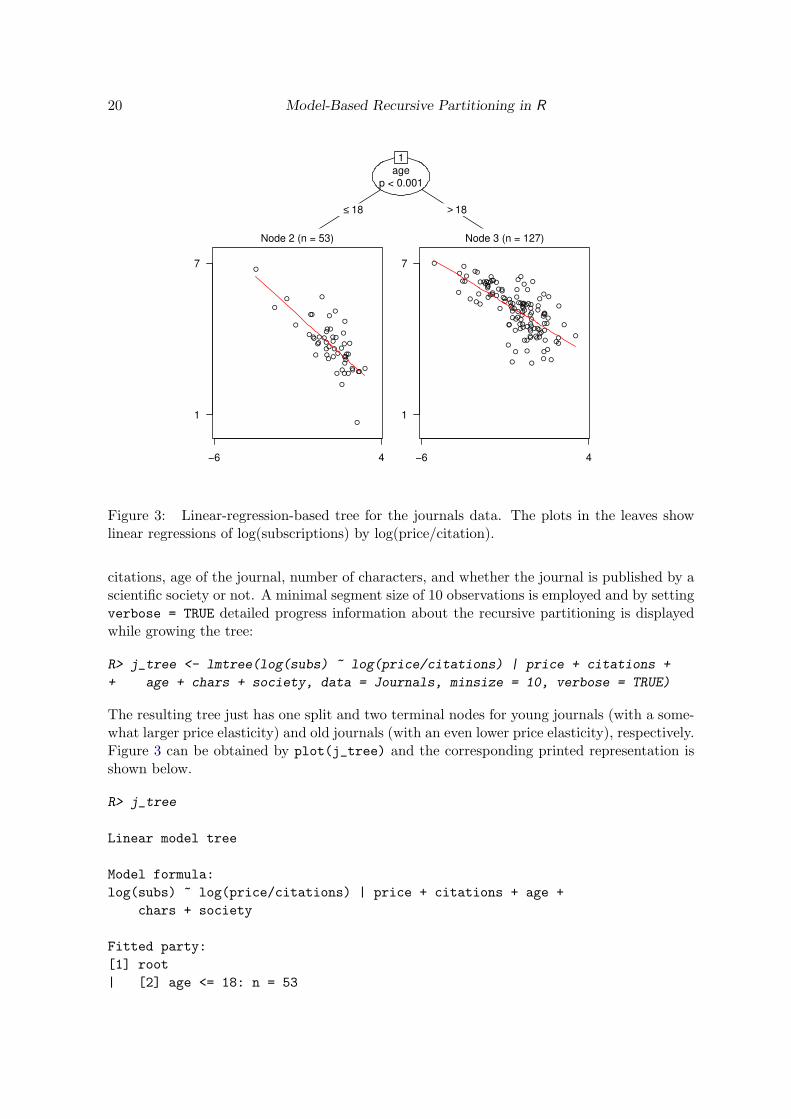
Figure 3: Linear-regression-based tree for the journals data. The plots in the leaves showlinear regressions of log(subscriptions) by log(price/citation).

citations, age of the journal, number of characters, and whether the journal is published by ascientific society or not. A minimal segment size of 10 observations is employed and by settingverbose = TRUE detailed progress information about the recursive partitioning is displayedwhile growing the tree:

R> j_tree <- lmtree(log(subs) ~ log(price/citations) | price + citations +

+ age + chars + society, data = Journals, minsize = 10, verbose = TRUE)

The resulting tree just has one split and two terminal nodes for young journals (with a some-what larger price elasticity) and old journals (with an even lower price elasticity), respectively.Figure 3 can be obtained by plot(j_tree) and the corresponding printed representation isshown below.

R> j_tree

Linear model tree

Model formula:

log(subs) ~ log(price/citations) | price + citations + age +

chars + society

Fitted party:

[1] root

| [2] age <= 18: n = 53


| (Intercept) log(price/citations)

| 4.3528 -0.6049

| [3] age > 18: n = 127

| (Intercept) log(price/citations)

| 5.011 -0.403




Objective function (residual sum of squares): 77.05

Finally, various quantities of interest such as the coefficients, standard errors and test statis-tics, and the associated parameter instability tests could be extracted by the following code.The corresponding output is suppressed here.

R> coef(j_tree, node = 1:3)

R> summary(j_tree, node = 1:3)

R> sctest(j_tree, node = 1:3)

4.2. Boston housing data

The Boston housing data are a popular and well-investigated empirical basis for illustratingnonlinear regression methods both in machine learning and statistics. We follow previousanalyses by segmenting a bivariate linear regression model for the house values.

The data set is available in package mlbench and can be obtained and transformed via:

R> data("BostonHousing", package = "mlbench")

R> BostonHousing <- transform(BostonHousing,

+ chas = factor(chas, levels = 0:1, labels = c("no", "yes")),

+ rad = factor(rad, ordered = TRUE))

It provides n = 506 observations of the median value of owner-occupied homes in Boston (inUSD 1000) along with 14 covariates including in particular the number of rooms per dwelling(rm) and the percentage of lower status of the population (lstat). A segment-wise linearrelationship between the value and these two variables is very intuitive, whereas the shapeof the influence of the remaining covariates is rather unclear and hence should be learnedfrom the data. Therefore, a linear regression model for median value explained by rm^2 andlog(lstat) is employed and partitioned with respect to all remaining variables. Choosingappropriate transformations of the dependent variable and the regressors that enter the linearregression model is important to obtain a well-fitting model in each segment and we follow inour choice the recommendations of Breiman and Friedman (1985). Monotonic transformationsof the partitioning variables do not affect the recursive partitioning algorithm and hence donot have to be performed. However, it is important to distinguish between numerical andcategorical variables for choosing an appropriate parameter stability test. The variable chas isa dummy indicator variable (for tract bounds with Charles river) and thus needs to be turnedinto a factor. Furthermore, the variable rad is an index of accessibility to radial highwaysand takes only 9 distinct values. Hence, it is most appropriately treated as an ordered factor.


Note that both transformations only affect the parameter stability test chosen (step 2), notthe splitting procedure (step 3).

R> bh_tree <- lmtree(medv ~ log(lstat) + I(rm^2) | zn + indus + chas + nox +

+ age + dis + rad + tax + crim + b + ptratio, data = BostonHousing)

R> bh_tree

Linear model tree

Model formula:

medv ~ log(lstat) + I(rm^2) | zn + indus + chas + nox + age +

dis + rad + tax + crim + b + ptratio

Fitted party:

[1] root

| [2] tax <= 432

| | [3] ptratio <= 15.2: n = 72

| | (Intercept) log(lstat) I(rm^2)

| | 9.2349 -4.9391 0.6859

| | [4] ptratio > 15.2

| | | [5] ptratio <= 19.6

| | | | [6] tax <= 265: n = 63

| | | | (Intercept) log(lstat) I(rm^2)

| | | | 3.9637 -2.7663 0.6881

| | | | [7] tax > 265: n = 162

| | | | (Intercept) log(lstat) I(rm^2)

| | | | -1.7984 -0.2677 0.6539

| | | [8] ptratio > 19.6: n = 56

| | | (Intercept) log(lstat) I(rm^2)

| | | 17.5865 -4.6190 0.3387

| [9] tax > 432: n = 153

| (Intercept) log(lstat) I(rm^2)

| 68.2971 -16.3540 -0.1478




Objective function (residual sum of squares): 6090

The corresponding visualization is shown in Figure 4. It shows partial scatter plots of thedependent variable against each of the regressors in the terminal nodes. Each scatter plotalso shows the fitted values, i.e., a projection of the fitted hyperplane.

From this visualization, it can be seen that in the nodes 4, 6, 7 and 8 the increase of value withthe number of rooms dominates the picture (upper panel) whereas in node 9 the decrease withthe lower status population percentage (lower panel) is more pronounced. Splits are performedin the variables tax (poperty-tax rate) and ptratio (pupil-teacher ratio).


tax

p <

0.0

01

1

≤4

32

>4

32

ptr

atio

p <

0.0

01

2

≤1

5.2

>1

5.2

No

de

3 (

n =

72

)

●●

●●● ● ●●●●● ●● ●●

●● ● ● ●● ●●● ● ●● ● ●● ● ●● ●●● ●●

●● ● ●●● ●● ● ●● ● ●●● ●● ●●● ● ●●●

● ●●● ●●● ●●●

0.3

3.9

1

54

●●●● ●●● ●● ●●●●● ●● ●● ●●●●● ● ● ●●●● ● ● ● ●●●

●●●● ● ● ●● ● ● ● ●●

● ● ●● ● ● ●●

●● ● ●●

● ●●●●●●

●● ●●

6.3

83

.5

1

54

ptr

atio

p <

0.0

01

4

≤1

9.6

>1

9.6

tax

p <

0.0

01

5

≤2

65

>2

65

No

de

6 (

n =

63

)

●● ●● ●●●

● ● ● ●● ● ●●● ●●● ● ●● ● ●●● ●● ●● ● ●●● ●● ● ●● ● ●● ●● ●● ●●● ●●● ●●● ●

● ●● ●

● ●●

0.3

3.9

1

54

●

●● ●●●●●● ●● ● ●●● ●● ●● ●●● ● ● ● ●●

● ●●● ● ●● ● ● ● ●●●● ●●● ●● ●● ●● ●●●● ●● ● ●●●

●●●

6.3

83

.5

1

54

No

de

7 (

n =

16

2)

●

●

●●● ●●●● ● ● ● ●● ●● ●●● ●● ●● ●●● ● ● ●● ● ● ●●● ●● ●● ●● ● ●● ●● ●● ● ●● ●● ●● ●●● ●●● ● ● ●●● ●● ●● ●●● ●● ● ●● ●● ●●● ●●● ● ●● ●● ● ●● ● ●● ● ●●● ●● ●● ●● ● ●● ●●●●● ● ●● ● ●● ● ●●● ●● ● ●● ●●●● ● ●●● ● ● ●● ● ●● ●● ●● ● ●●● ●● ●●●● ● ●

●

0.3

3.9

1

54

●● ● ●● ●● ● ●●● ●●● ●●●● ●● ●● ●●● ●● ●●● ●●● ● ●● ●● ●●●●●● ●● ● ●●● ●● ●●●● ● ●● ●●● ● ●●● ● ●●●● ●● ●● ●●● ● ●●● ●●●● ●● ●● ● ●●● ●●● ● ●● ●● ●●● ●● ● ●●●● ● ●● ●● ● ●●● ●●● ●● ● ●●● ● ● ●●● ●●● ● ●●●● ● ●●●● ●

● ●●●

●●

●●

● ●● ●

●

6.3

83

.5

1

54

No

de

8 (

n =

56

)

●● ●● ● ●● ● ●●

● ●● ●● ●●● ● ●● ● ● ●● ●●●

●●● ●●●● ●●●●●

●● ●● ●● ●●●● ● ● ●

● ●●

0.3

3.9

1

54

● ●●● ● ●●● ●●● ●●● ● ●●● ● ● ●● ●●● ● ●● ●● ●● ●● ● ● ●● ●● ●●● ●● ●● ●● ●● ●● ●

● ●

6.3

83

.5

1

54

No

de

9 (

n =

15

3)

●●

●

●●● ●●

●●

●● ●● ●●● ●●● ●● ● ●● ●●●●● ● ● ●●● ● ●●● ●● ●●●● ●● ●● ● ●● ●●●●● ●● ●● ● ● ●● ● ●● ●● ●● ● ●● ●● ● ● ●● ●●●● ●●● ● ●● ● ●● ●● ● ●● ●● ● ●●● ●● ●●● ● ●● ●● ●● ●● ● ●● ● ●● ●●● ●● ● ● ●● ●● ●●● ●● ● ●● ● ●●●● ● ● ●●

0.3

3.9

1

54

●

●

● ●● ●● ●

●●●● ●● ● ●● ●●● ●● ● ●● ●● ● ●●●● ● ●●● ●● ●● ●● ●●● ● ●● ● ●●●●● ●● ●● ● ●●●● ●●●● ●● ●● ● ●● ●● ● ●●● ●●● ● ● ●●● ●● ● ●●●● ● ●● ●● ●● ● ● ●●● ● ● ●●● ●●● ● ●●● ●●● ●● ● ●●● ●● ● ●●●●●● ● ● ●● ●● ●●● ●●● ●

●●

●

6.3

83

.5

1

54

Figure 4: Linear-regression-based tree for the Boston housing data. The plots in the leavesgive partial scatter plots for rm (upper panel) and lstat (lower panel).


For summarizing the quality of the fit, we could compute the mean squared error, log-likelihood or AIC:

R> mean(residuals(bh_tree)^2)

[1] 12.04

R> logLik(bh_tree)

✬log Lik.✬ -1311 (df=24)

R> AIC(bh_tree)

[1] 2669

4.3. Teaching ratings data

Hamermesh and Parker (2005) investigate the correlation of beauty and teaching evaluationsfor professors. They provide data on course evaluations, course characteristics, and professorcharacteristics for 463 courses for the academic years 2000–2002 at the University of Texasat Austin. It is of interest how the average teaching evaluation per course (on a scale 1–5)depends on a standardized measure of beauty (as assessed by a committee of six personsbased on photos). Hamermesh and Parker (2005) employ a linear regression, weighted by thenumber of students per course and adjusting for several further main effects: gender, whetheror not the teacher is from a minority, a native speaker, or has tenure, respectively, and whetherthe course is taught in the upper or lower division. Additionally, the age of the professorsis available as a regressor but not considered by Hamermesh and Parker (2005) because thecorresponding main effect is not found to be significant in either linear or quadratic form.

Here, we employ a similar model but use the available regressors differently. The basic modelis again a linear regression for teaching rating by beauty, estimated by weighted least squares(WLS). All remaining explanatory variables are not used as regressors but as partitioningvariables because we argue that it is unclear how they influence the correlation betweenteaching rating and beauty. Hence, MOB is used to adaptively incorporate these furthervariables and determine potential interactions.

First, the data are loaded from the AER package (Kleiber and Zeileis 2008) and only thesubset of single-credit courses is excluded.

R> data("TeachingRatings", package = "AER")

R> tr <- subset(TeachingRatings, credits == "more")

The single-credit courses include elective modules that are quite different from the remainingcourses (e.g., yoga, aerobics, or dance) and are hence omitted from the main analysis.

WLS estimation of the null model (with only an intercept) and the main effects model iscarried out in a first step:


R> tr_null <- lm(eval ~ 1, data = tr, weights = students)

R> tr_lm <- lm(eval ~ beauty + gender + minority + native + tenure + division,

+ data = tr, weights = students)

Then, the model-based tree can be estimated with lmtree() using only beauty as a regressorand all remaining variables for partitioning. For WLS estimation, we set weights = students

and caseweights = FALSE (because the weights are only proportionality factors and do notsignal exactly replicated observations).

R> (tr_tree <- lmtree(eval ~ beauty | minority + age + gender + division +

+ native + tenure, data = tr, weights = students, caseweights = FALSE))

Linear model tree

Model formula:

eval ~ beauty | minority + age + gender + division + native +

tenure

Fitted party:

[1] root

| [2] gender in female

| | [3] age <= 40: n = 69

| | (Intercept) beauty

| | 4.0137 0.1222

| | [4] age > 40

| | | [5] division in lower: n = 36

| | | (Intercept) beauty

| | | 3.5900 0.4033

| | | [6] division in upper: n = 81

| | | (Intercept) beauty

| | | 3.7752 -0.1976

| [7] gender in male

| | [8] age <= 50: n = 113


| | 3.9968 0.1292

| | [9] age > 50: n = 137


| | 4.0857 0.5028




Objective function (residual sum of squares): 2752

The resulting tree can be visualized by plot(tr_tree) and is shown in Figure 5. This showsthat despite age not having a significant main effect (as reported by Hamermesh and Parker2005), it clearly plays an important role: While the correlation of teaching rating and beauty


gender

p < 0.001

1

female male

age

p = 0.014

2

≤ 40 > 40

Node 3 (n = 69)

●

●

●●

●●

●

●

●●

●●

●

●

●

●

●

●●●

●

●●●●

●

●

●

●

●

●

●

●●

●●

●

●

●

●

●

●

●●

●

●

● ●

●

●

●

●

●

●●

●

●●●●

●

●

●

●

●

●

●●

●

−1.7 2.3

2

5

division

p = 0.019

4

lower upper

Node 5 (n = 36)

●●●●●

●

●

●

●

●

●

●

●

●

●

●

●

●●

●

●●

●●

●●

●

●

●

●

●●

●

●

●

●

−1.7 2.3

2

5

Node 6 (n = 81)

●

●●

●●

●

●

●

●

●

●

●

●●

●

●

●

●●

●●

●

●

●●●

●

●

●●

●

●

●

●

●

●

●

●●●●

●

●

●

●

●

●●

●●

●

●●

●●

●

●●

●

●●

●

●

●

●●●

●

●●●

●

●

●

●

●

●

●

●

●

●

−1.7 2.3

2

5

age

p = 0.008

7

≤ 50 > 50

Node 8 (n = 113)

●

●

●

●

●

●

●

●

●

●

●

●

●

●

●

●

●

●●●

●

●●

●●●

●

●

●

●

●

●

●

●

●

●●

●

●●●

●

●

●●

●

●

●

●●

●●

●

●

●●●

●

●

●

●●●

●

●

●

●

●

●

●

●

●

●

●

●●

●●

●●

●

●

●

●

●

●

●

●

●●●

●

●

●●●

●

●

●

●●

●●

●

●

●

●

●

●

●

●

●●

−1.7 2.3

2

5

Node 9 (n = 137)

●

●

●

●

●●●

●

●

●

●●●

●●

●

●

●

●●●

●

●

●●

●

●

●

●

●

●

●●

●

●

●

●

●

●

●

●

●

●

●●

●

●

●

●

●

●

●

●●

●●

●

●

●

●

●

●

●

●

●

●

●

●

●

●●●●

●

●

●

●●●

●

●●

●●●

●

●●

●

●

●

●

●

●

●

●

●

●●

●

●●

●

●●●●

●

●●

●

●

●

●●●

●

●

●

●●●

●

●

●●●●● ●

●●

●●

●

●

●

−1.7 2.3

2

5

Figure 5: WLS-based tree for the teaching ratings data. The plots in the leaves showscatterplots for teaching rating by beauty score.

score is rather moderate for younger professors, there is a clear correlation for older professors(with the cutoff age somewhat lower for female professors).

R> coef(tr_lm)[2]

beauty

0.2826

R> coef(tr_tree)[, 2]

3 5 6 8 9

0.1222 0.4033 -0.1976 0.1292 0.5028

Th R2 of the tree is also clearly improved over the main effects model:

R> 1 - c(deviance(tr_lm), deviance(tr_tree))/deviance(tr_null)

[1] 0.2713 0.3820

4.4. Titanic survival data

To illustrate how differences in treatment effects can be captured by MOB, the Titanic survivaldata is considered: The question is whether “women and children first” is applied in the same


way for all subgroups of the passengers of the Titanic. Or, in other words, whether theeffectiveness of preferential treatment for women/children differed across subgroups.

The Titanic data is provided in base R as a contingency table and transformed here to a‘data.frame’ for use with glmtree():

R> data("Titanic", package = "datasets")

R> ttnc <- as.data.frame(Titanic)

R> ttnc <- ttnc[rep(1:nrow(ttnc), ttnc$Freq), 1:4]

R> names(ttnc)[2] <- "Gender"

R> ttnc <- transform(ttnc, Treatment = factor(

+ Gender == "Female" | Age == "Child", levels = c(FALSE, TRUE),

+ labels = c("Male&Adult", "Female|Child")))

The data provides factors Survived (yes/no), Class (1st, 2nd, 3rd, crew), Gender (male,female), and Age (child, adult). Additionally, a factor Treatment is added that distinguisheswomen/children from male adults.

To investigate how the preferential treatment effect (Survived ~ Treatment) differs acrossthe remaining explanatory variables, the following logistic-regression-based tree is considered.The significance level of alpha = 0.01 is employed here to avoid overfitting and separationproblems in the logistic regression.

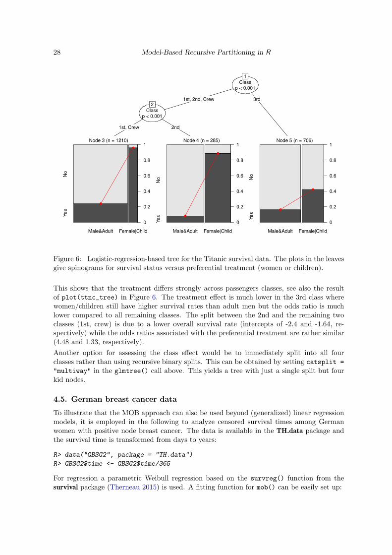
R> ttnc_tree <- glmtree(Survived ~ Treatment | Class + Gender + Age,

+ data = ttnc, family = binomial, alpha = 0.01)

R> ttnc_tree

Generalized linear model tree (family: binomial)

Model formula:

Survived ~ Treatment | Class + Gender + Age

Fitted party:

[1] root

| [2] Class in 1st, 2nd, Crew

| | [3] Class in 1st, Crew: n = 1210

| | (Intercept) TreatmentFemale|Child

| | -1.152 4.318

| | [4] Class in 2nd: n = 285

| | (Intercept) TreatmentFemale|Child

| | -2.398 4.477

| [5] Class in 3rd: n = 706

| (Intercept) TreatmentFemale|Child

| -1.641 1.327




Objective function (negative log-likelihood): 1061


Class

p < 0.001

1

1st, 2nd, Crew 3rd

Class

p < 0.001

2

1st, Crew 2nd

Node 3 (n = 1210)

Male&Adult Female|Child

Yes

No

0

0.2

0.4

0.6

0.8

1

●

●

Node 4 (n = 285)


Yes

No

0

0.2

0.4

0.6

0.8

1

●

●

Node 5 (n = 706)


Yes

No

0

0.2

0.4

0.6

0.8

1

●

●

Figure 6: Logistic-regression-based tree for the Titanic survival data. The plots in the leavesgive spinograms for survival status versus preferential treatment (women or children).

This shows that the treatment differs strongly across passengers classes, see also the resultof plot(ttnc_tree) in Figure 6. The treatment effect is much lower in the 3rd class wherewomen/children still have higher survival rates than adult men but the odds ratio is muchlower compared to all remaining classes. The split between the 2nd and the remaining twoclasses (1st, crew) is due to a lower overall survival rate (intercepts of -2.4 and -1.64, re-spectively) while the odds ratios associated with the preferential treatment are rather similar(4.48 and 1.33, respectively).

Another option for assessing the class effect would be to immediately split into all fourclasses rather than using recursive binary splits. This can be obtained by setting catsplit =

"multiway" in the glmtree() call above. This yields a tree with just a single split but fourkid nodes.

4.5. German breast cancer data

To illustrate that the MOB approach can also be used beyond (generalized) linear regressionmodels, it is employed in the following to analyze censored survival times among Germanwomen with positive node breast cancer. The data is available in the TH.data package andthe survival time is transformed from days to years:

R> data("GBSG2", package = "TH.data")

R> GBSG2$time <- GBSG2$time/365

For regression a parametric Weibull regression based on the survreg() function from thesurvival package (Therneau 2015) is used. A fitting function for mob() can be easily set up:


R> library("survival")

R> wbreg <- function(y, x, start = NULL, weights = NULL, offset = NULL, ...) {

+ survreg(y ~ 0 + x, weights = weights, dist = "weibull", ...)

+ }

As the survreg package currently does not provide a logLik() method for ‘survreg’ objects,this needs to be added here:

R> logLik.survreg <- function(object, ...)

+ structure(object$loglik[2], df = sum(object$df), class = "logLik")

Without the logLik() method, mob() would not know how to extract the optimized objectivefunction from the fitted model.

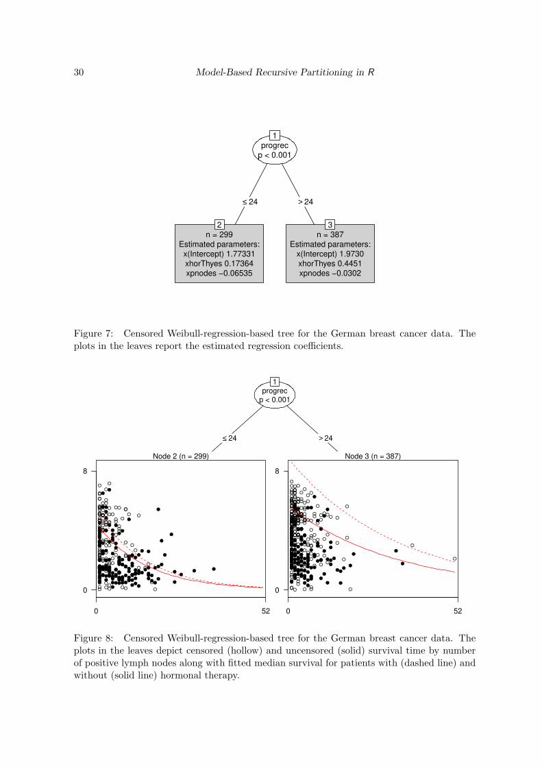
With the functions above available, a censored Weibull-regression-tree can be fitted: Thedependent variable is the censored survival time and the two regressor variables are the mainrisk factor (number of positive lymph nodes) and the treatment variable (hormonal therapy).All remaining variables are used for partitioning: age, tumor size and grade, progesterone andestrogen receptor, and menopausal status. The minimal segment size is set to 80.

R> gbsg2_tree <- mob(Surv(time, cens) ~ horTh + pnodes | age + tsize +

+ tgrade + progrec + estrec + menostat, data = GBSG2,

+ fit = wbreg, control = mob_control(minsize = 80))

Based on progesterone receptor, a tree with two leaves is found:

R> gbsg2_tree

Model-based recursive partitioning (wbreg)

Model formula:

Surv(time, cens) ~ horTh + pnodes | age + tsize + tgrade + progrec +

estrec + menostat

Fitted party:

[1] root

| [2] progrec <= 24: n = 299

| x(Intercept) xhorThyes xpnodes

| 1.77331 0.17364 -0.06535

| [3] progrec > 24: n = 387

| x(Intercept) xhorThyes xpnodes

| 1.9730 0.4451 -0.0302





R> coef(gbsg2_tree)


progrec

p < 0.001

1

≤ 24 > 24

n = 299


x(Intercept) 1.77331

xhorThyes 0.17364

xpnodes −0.06535

2

n = 387


x(Intercept) 1.9730

xhorThyes 0.4451

xpnodes −0.0302

3

Figure 7: Censored Weibull-regression-based tree for the German breast cancer data. Theplots in the leaves report the estimated regression coefficients.

progrec

p < 0.001

1

≤ 24 > 24

Node 2 (n = 299)

● ●

●

●

●

●

●

●

●

● ●●

●

●

●

●

●

●

●

●

●

●

●

●

●●

●

●

●

●

●

●

●

● ●

●

●

●

●

● ●

●

●

●

●

●

●

●

●

●●

●

●

●●

●

●

●

●

●

●

●

●

●

●●

●

●

●

●

●

●

●

●

●

●

●

●

●

●

●

●●

●

●●

●

●

●

●

●●

●

●

●●

●

●

●

● ●

●

●

●

●

●

●

●

●

●

●

●

●●

●

●

●

●

● ●

●

●

●

●

●

●

●

●

●

●

●

●

●

●

●

●

●

● ●

●

●

●

●

●

●

●●

●

●

●

●

●

●

●

●

●

●

●

●

●

●

●

●

●

●

●

●

●

●

●

●

●

●

●

●●

●

●

●

●

●

●

●

●

●

●

●

●

●

●

●●

●

●

●

●

●

●

●

●

●●

●

●

●

●

●

●

●

●

●

●

●

●

●

●

●

●

●●

●

●

●

●

●

●

●

●

●

●●

●

●

●

●

●●

●

●●●●

●

●

●

●

●

●

●

●

●

●●

●

●

●

●

●

●

●

●

●

●

●

●

●●

●

●

●

●

●●

●

●●

●

●

● ●

●

●

●

● ●●

●

●

●

●

●●●

●

●●

●

●

●

0 52

0

8

Node 3 (n = 387)

●

●

●

●

●

●●

● ●

●

●

●●

●

● ● ●

●

●

●

● ●

●

●●●

● ●

●

●

●

●

●

●

●

●

●

●

●

●

●

●

●

●

●

●

●●

●

●

●

●

●

●

●●

●●

●

●

●●

●

●

●

●●

●

●

●

●

●

●

●

●

●

●

●

●

●

●

●

●●

●

●

●

●●

●●

●

●

●

●

●

●

●

●

●

●

●

●

●

●

● ●

●

●

●

●●

●

●

●

●●

●

●●

●

●

●●

●●

●

●

●

●

●

●

●●

●●

●●

●

●

●

●

●

●

●

●

●

●

●

●

●

●●

●

●

●

●

●●

●●

●

●

●

●

●

●

●

●

●

●●

●

●

●

●

●

●●

●

●

●

●

●

●

● ●

●

●

●

●

●

●

●

●

●

●●

●

●

●

●●

●

●

●●●

●●

●

●

●

●

●

●

●

●●

●

●

●●

●

● ●●

●

●

●

●

●

●

●

●

●

●

●

●●

●●

●

●

● ●●

●●

●

●

●

●

●

●

●

●

●

●●

●

●

●

●

●

●

●

●

●

●

●

●

●●

●

●

●

●

●●

●

●

●

●

●

●●

●

●

●●●●

●

●

●

●

●

●●

●

●

●

●●

●

●

● ●

●●

●●

●

●●●

●

●

●

●

●●

●

●

●

●

●

●

●

●

●

● ●

●●

●

●

●

●

●

●

●

●●

●

●●

●

●

●●

●

●●

●

●●

●

●

●

●

● ●

●

●●●●

●●

●

●●● ●●

●

●

●

●●

● ●●

●

●

0 52

0

8

Figure 8: Censored Weibull-regression-based tree for the German breast cancer data. Theplots in the leaves depict censored (hollow) and uncensored (solid) survival time by numberof positive lymph nodes along with fitted median survival for patients with (dashed line) andwithout (solid line) hormonal therapy.


x(Intercept) xhorThyes xpnodes

2 1.773 0.1736 -0.06535

3 1.973 0.4451 -0.03020

R> logLik(gbsg2_tree)

✬log Lik.✬ -809.9 (df=9)

The visualization produced by plot(gbsg2_tree) is shown in Figure 7. A nicer graphicaldisplay using a scatter plot (with indication of censoring) and fitted regression curves is shownin Figure 8. This uses a custom panel function whose code is too long and elaborate to beshown here. Interested readers are referred to the R code underlying the vignette.

The visualization shows that for higher progesterone receptor levels: (1) survival times arehigher overall, (2) the treatment effect of hormonal therapy is higher, and (3) the negativeeffect of the main risk factor (number of positive lymph nodes) is less severe.

5. Setting up a new mobster

To conclude this vignette, we present another illustration that shows how to set up newmobster functionality from scratch. To do so, we implement the Bradley-Terry tree suggestedby Strobl et al. (2011) “by hand”. The psychotree package already provides an easy-to-usemobster called bttree() but as an implementation exercise we recreate its functionality here.

The only inputs required are a suitable data set with paired comparisons (Topmodel2007 frompsychotree) and a parametric model for paired comparison data (btmodel() from psychotools,implementing the Bradley-Terry model). The latter optionally computes the empirical esti-mating functions and already comes with a suitable extractor method.

R> data("Topmodel2007", package = "psychotree")

R> library("psychotools")

The Bradley-Terry (or Bradley-Terry-Luce) model is a standard model for paired comparisonsin social sciences. It parametrizes the probability πij for preferring some object i over anotherobject j in terms of corresponding “ability” or “worth” parameters θi:

πij =θi

θi + θj

logit(πij) = log(θi)− log(θj)

This model can be easily estimated by maximum likelihood as a logistic or log-linear GLM.This is the approach used internally by btmodel().

The Topmodel2007 data provide paired comparisons of attractiveness among the six finalistsof the TV show Germany’s Next Topmodel 2007 : Barbara, Anni, Hana, Fiona, Mandy, Anja.The data were collected in a survey with 192 respondents at Universitat Tubingen and theavailable covariates comprise gender, age, and familiarty with the TV show. The latter isassess by three by yes/no questions: (1) Do you recognize the women?/Do you know theshow? (2) Did you watch it regularly? (3) Did you watch the final show?/Do you know whowon?


To fit the Bradley-Terry tree to the data, the available building blocks just have to be tiedtogether. First, we set up the basic/simple model fitting interface described in Section 3.2:

R> btfit1 <- function(y, x = NULL, start = NULL, weights = NULL,

+ offset = NULL, ...) btmodel(y, ...)

The function btfit1() simply calls btmodel() ignoring all arguments except y as the othersare not needed here. No more processing is required because ‘btmodel’ objects come witha coef(), logLik(), and estfun() method. Hence, we can call mob() now specifying theresponse and the partitioning variable (and no regressors because there are no regressors inthis model).

R> bt1 <- mob(preference ~ 1 | gender + age + q1 + q2 + q3,

+ data = Topmodel2007, fit = btfit1)

An alternative way to fit the exact same tree somewhat more quickly would be to employ theextended interface described in Section 3.2:

R> btfit2 <- function(y, x = NULL, start = NULL, weights = NULL,

+ offset = NULL, ..., estfun = FALSE, object = FALSE) {

+ rval <- btmodel(y, ..., estfun = estfun, vcov = object)

+ list(

+ coefficients = rval$coefficients,

+ objfun = -rval$loglik,

+ estfun = if(estfun) rval$estfun else NULL,

+ object = if(object) rval else NULL

+ )

+ }

Still btmodel() is employed for fitting the model but the quantities estfun and vcov are onlycomputed if they are really required. This may save some computation time – about 20% onthe authors’ machine at the time of writing – when computing the tree:

R> bt2 <- mob(preference ~ 1 | gender + age + q1 + q2 + q3,

+ data = Topmodel2007, fit = btfit2)

The speed-up is not huge but comes almost for free: just a few additional lines of code inbtfit2() are required. For other models where it is more costly to set up a full model (withvariance-covariance matrix, predictions, residuals, etc.) larger speed-ups are also possible.

Both trees, bt1 and bt2, are equivalent (except for the details of the fitting function). Hence,in the following we only explore bt2. However, the same code can be applied to bt1 as well.

Many tools come completely for free and are inherited from the general ‘modelparty’/‘party’.For example, both printing (print(bt2)) and plotting (plot(bt2)) shows the estimatedparameters in the terminal nodes which can also be extracted by the coef() method:

R> bt2


Model-based recursive partitioning (btfit2)

Model formula:

preference ~ 1 | gender + age + q1 + q2 + q3

Fitted party:

[1] root

| [2] age <= 52

| | [3] q2 in no

| | | [4] gender in female: n = 56

| | | Barbara Anni Hana Fiona Mandy

| | | 0.9475 0.7246 0.4452 0.6350 -0.4965

| | | [5] gender in male: n = 71

| | | Barbara Anni Hana Fiona Mandy

| | | 0.43866 0.08877 0.84629 0.69424 -0.10003

| | [6] q2 in yes: n = 35

| | Barbara Anni Hana Fiona Mandy

| | 1.3378 1.2318 2.0499 0.8339 0.6217

| [7] age > 52: n = 30

| Barbara Anni Hana Fiona Mandy

| 0.2178 -1.3166 -0.3059 -0.2591 -0.2357




Objective function: 1829

R> coef(bt2)

Barbara Anni Hana Fiona Mandy

4 0.9475 0.72459 0.4452 0.6350 -0.4965

5 0.4387 0.08877 0.8463 0.6942 -0.1000

6 1.3378 1.23183 2.0499 0.8339 0.6217

7 0.2178 -1.31663 -0.3059 -0.2591 -0.2357

The corresponding visualization is shown in the upper panel of Figure 9. In all cases, theestimated coefficients on the logit scale omitting the fixed zero reference level (Anja) arereported. To show the corresponding worth parameters θi including the reference level, onecan simply provide a small panel function worthf(). This applies the worth() function frompsychotools to the fitted-model object stored in the info slot of each node, yielding the lowerpanel in Figure 9.

R> worthf <- function(info) paste(info$object$labels,

+ format(round(worth(info$object), digits = 3)), sep = ": ")

R> plot(bt2, FUN = worthf)

To show a graphical display of these worth parameters rather than printing their numericalvalues, one can use a simply glyph-style plot. A simply way to generate these is to use the


age

p < 0.001

1

≤ 52 > 52

q2

p = 0.017

2

no yes

gender

p = 0.007

3

female male

n = 56


Barbara 0.9475

Anni 0.7246

Hana 0.4452

Fiona 0.6350

Mandy −0.4965

4

n = 71


Barbara 0.43866

Anni 0.08877

Hana 0.84629

Fiona 0.69424

Mandy −0.10003

5

n = 35


Barbara 1.3378

Anni 1.2318

Hana 2.0499

Fiona 0.8339

Mandy 0.6217

6

n = 30


Barbara 0.2178

Anni −1.3166

Hana −0.3059

Fiona −0.2591

Mandy −0.2357

7

age

p < 0.001

1

≤ 52 > 52

q2

p = 0.017

2

no yes

gender

p = 0.007

3

female male

Barbara: 0.266

Anni: 0.213

Hana: 0.161

Fiona: 0.195

Mandy: 0.063

Anja: 0.103

4

Barbara: 0.175

Anni: 0.123

Hana: 0.262

Fiona: 0.225

Mandy: 0.102

Anja: 0.113

5

Barbara: 0.189

Anni: 0.170

Hana: 0.385

Fiona: 0.114

Mandy: 0.092

Anja: 0.050

6

Barbara: 0.259

Anni: 0.056

Hana: 0.153

Fiona: 0.160

Mandy: 0.164

Anja: 0.208

7

Figure 9: Bradley-Terry-based tree for the topmodel attractiveness data. The default plot(upper panel) reports the estimated coefficients on the log scale while the adapted plot (lowerpanel) shows the corresponding worth parameters.


3

Objects

Wort

h p

ara

mete

rs

0.0

0.1

0.2

0.3

0.4

●

●

● ●

●

●

Barbara Anni Hana Fiona Mandy Anja

5

Objects

Wort

h p

ara

mete

rs

0.0

0.1

0.2

0.3

0.4

●

●

●

●

●●


6

Objects

Wort

h p

ara

mete

rs

0.0

0.1

0.2

0.3

0.4

●●

●

●●

●


7

Objects

Wort

h p

ara

mete

rs

0.0

0.1

0.2

0.3

0.4

●

●

● ● ●

●


Figure 10: Worth parameters in the terminal nodes of the Bradley-Terry-based tree for thetopmodel attractiveness data.

plot() method for ‘btmodel’ objects from partykit and nodeapply this to all terminal nodes(see Figure 10):

R> par(mfrow = c(2, 2))

R> nodeapply(bt2, ids = c(3, 5, 6, 7), FUN = function(n)

+ plot(n$info$object, main = n$id, ylim = c(0, 0.4)))

Alternatively, one could set up a proper panel-generating function in grid that allows to createthe glyphs within the terminal nodes of the tree (see Figure 11). As the code for this panel-generating function node_btplot() is too complicated to display within the vignette, we referinterested readers to the underlying code. Given this panel-generating function Figure 11 canbe generated with

R> plot(bt2, drop = TRUE, tnex = 2,

+ terminal_panel = node_btplot(bt2, abbreviate = 1, yscale = c(0, 0.5)))

Finally, to illustrate how different predictions can be easily computed, we set up a small dataset with three new individuals:


age

p < 0.001

1

≤ 52 > 52

q2

p = 0.017

2

no yes

gender

p = 0.007

3

female male

Node 4 (n = 56)

●

●

●

●

●

●

B Ann H F M Anj

0

0.5Node 5 (n = 71)

●

●

●

●

● ●

B Ann H F M Anj

0

0.5Node 6 (n = 35)

●●

●

●●

●

B Ann H F M Anj

0

0.5Node 7 (n = 30)

●

●

● ● ●

●

B Ann H F M Anj

0

0.5

Figure 11: Bradley-Terry-based tree for the topmodel attractiveness data with visualizationsof the worth parameters in the terminal nodes.

age gender q1 q2 q3

1 60 male no no no

2 25 female no no no

3 35 female no yes no

For these we can easily compute (1) the predicted node ID, (2) the corresponding worthparameters, (3) the associated ranks.

R> tm

age gender q1 q2 q3

1 60 male no no no

2 25 female no no no

3 35 female no yes no

R> predict(bt2, tm, type = "node")

1 2 3

7 6 5

R> predict(bt2, tm, type = function(object) t(worth(object)))



1 0.2585 0.05573 0.1531 0.1605 0.16427 0.20792

2 0.1889 0.16993 0.3851 0.1142 0.09232 0.04958

3 0.1746 0.12305 0.2625 0.2254 0.10188 0.11259

R> predict(bt2, tm, type = function(object) t(rank(-worth(object))))


1 1 6 5 4 3 2

2 2 3 1 4 5 6

3 3 4 1 2 6 5

This completes the tour of fitting, printing, plotting, and predicting the Bradley-Terry treemodel. Convenience interfaces that employ code like shown above can be easily defined andcollected in new packages such as psychotree.

6. Conclusion

The function mob() in the partykit package provides a new flexible and object-oriented im-plementation of the general algorithm for model-based recursive partitioning using partykit’srecursive partytioning infrastructure. New model fitting functions can be easily provided,especially if standard extractor functions (such as coef(), estfun(), logLik(), etc.) areavailable. The resulting model trees can then learned, visualized, investigated, and employedfor predictions. To gain some efficiency in the computations and to allow for further customiza-tion (in particular specialized visualization and prediction methods), convenience interfaceslmtree() and glmtree() are provided for recursive partitioning based on (generalized) linearmodels.

References

Bache K, Lichman M (2013). “UCI Machine Learning Repository.” URL http://archive.

ics.uci.edu/ml/.

Bai J, Perron P (2003). “Computation and Analysis of Multiple Structural Change Models.”Journal of Applied Econometrics, 18, 1–22.

Breiman L, Friedman JH (1985). “Estimating Optimal Transformations for Multiple Regres-sion and Correlation.” Journal of the American Statistical Association, 80(391), 580–598.

Genz A, Bretz F, Miwa T, Mi X, Leisch F, Scheipl F, Hothorn T (2015). mvtnorm: Multivari-

ate Normal and t Distributions. R package version 1.0-3, URL http://CRAN.R-project.

org/package=mvtnorm.

Grun B, Kosmidis I, Zeileis A (2012). “Extended Beta Regression in R: Shaken, Stirred,Mixed, and Partitioned.” Journal of Statistical Software, 48(11), 1–25. URL http://www.

jstatsoft.org/v48/i11/.

http://archive.ics.uci.edu/ml/

http://archive.ics.uci.edu/ml/

http://CRAN.R-project.org/package=mvtnorm

http://CRAN.R-project.org/package=mvtnorm

http://www.jstatsoft.org/v48/i11/



Hamermesh DS, Parker A (2005). “Beauty in the Classroom: Instructors’ Pulchritude andPutative Pedagogical Productivity.” Economics of Education Review, 24, 369–376.

Hansen BE (1997). “Approximate Asymptotic p Values for Structural-Change Tests.” Journalof Business & Economic Statistics, 15, 60–67.

Hawkins DM (2001). “Fitting Multiple Change-Point Models to Data.” Computational Statis-

tics & Data Analysis, 37, 323–341.

Hothorn T, Hornik K, Strobl C, Zeileis A (2015). party: A Laboratory for Recursive Party-

tioning. R package version 1.0-23, URL http://CRAN.R-project.org/package=party.

Hothorn T, Leisch F, Zeileis A (2013). modeltools: Tools and Classes for Statistical Models.R package version 0.2-21, URL http://CRAN.R-project.org/package=modeltools.

Hothorn T, Zeileis A (2015). partykit: A Toolkit for Recursive Partytioning. R packageversion 1.0-3, URL http://CRAN.R-project.org/package=partykit.

Kleiber C, Zeileis A (2008). Applied Econometrics with R. Springer-Verlag, New York. URLhttp://CRAN.R-project.org/package=AER.

Leisch F, Dimitriadou E (2012). mlbench: Machine Learning Benchmark Problems. R

package version 2.1-1, URL http://CRAN.R-project.org/package=mlbench.

Merkle EC, Fan J, Zeileis A (2014). “Testing for Measurement Invariance with Respect to anOrdinal Variable.” Psychometrika, 79(4), 569–584. doi:10.1007/S11336-013-9376-7.

Merkle EC, Zeileis A (2013). “Tests of Measurement Invariance without Subgroups: A Gen-eralization of Classical Methods.” Psychometrika, 78(1), 59–82.

Meyer D, Zeileis A, Hornik K (2006). “The Strucplot Framework: Visualizing Multi-WayContingency Tables with vcd.” Journal of Statistical Software, 17(3), 1–48. URL http:

//www.jstatsoft.org/v17/i03/.

R Core Team (2013). R: A Language and Environment for Statistical Computing. R Founda-tion for Statistical Computing, Vienna, Austria. URL http://www.R-project.org/.

Strobl C, Kopf J, Zeileis A (2015). “Rasch Trees: A New Method for Detecting DifferentialItem Functioning in the Rasch Model.” Psychometrika, 80(2), 289–316. doi:10.1007/

s11336-013-9388-3.

Strobl C, Wickelmaier F, Zeileis A (2011). “Accounting for Individual Differences in Bradley-Terry Models by Means of Recursive Partitioning.” Journal of Educational and Behavioral

Statistics, 36(2), 135–153.

Su X, Wang M, Fan J (2004). “Maximum Likelihood Regression Trees.” Journal of Compu-

tational and Graphical Statistics, 13, 586–598.

Therneau TM (2015). survival: A Package for Survival Analysis in S. R package version2.38-3, URL http://CRAN.R-project.org/package=survival.

Zeileis A (2005). “A Unified Approach to Structural Change Tests Based on ML Scores,F Statistics, and OLS Residuals.” Econometric Reviews, 24, 445–466.

http://CRAN.R-project.org/package=party

http://CRAN.R-project.org/package=modeltools

http://CRAN.R-project.org/package=partykit

http://CRAN.R-project.org/package=AER

http://CRAN.R-project.org/package=mlbench

http://dx.doi.org/10.1007/S11336-013-9376-7



http://www.R-project.org/

http://dx.doi.org/10.1007/s11336-013-9388-3

http://dx.doi.org/10.1007/s11336-013-9388-3

http://CRAN.R-project.org/package=survival


Zeileis A (2006). “Object-Oriented Computation of Sandwich Estimators.” Journal of Statis-

tical Software, 16(9), 1–16. URL http://www.jstatsoft.org/v16/i09/.

Zeileis A, Croissant Y (2010). “Extended Model Formulas in R: Multiple Parts and MultipleResponses.” Journal of Statistical Software, 34(1), 1–13. URL http://www.jstatsoft.

org/v34/i01/.

Zeileis A, Hornik K (2007). “Generalized M-Fluctuation Tests for Parameter Instability.”Statistica Neerlandica, 61(4), 488–508.

Zeileis A, Hothorn T, Hornik K (2008). “Model-Based Recursive Partitioning.” Journal of

Computational and Graphical Statistics, 17(2), 492–514.

Zeileis A, Leisch F, Hornik K, Kleiber C (2002). “strucchange: An R Package for Testingfor Structural Change in Linear Regression Models.” Journal of Statistical Software, 7(2),1–38. URL http://www.jstatsoft.org/v07/i02/.

Affiliation:

Achim ZeileisDepartment of StatisticsFaculty of Economics and StatisticsUniversitat InnsbruckUniversitatsstr. 156020 Innsbruck, AustriaE-mail: [email protected]: http://eeecon.uibk.ac.at/~zeileis/

Torsten HothornInstitut fur Epidemiologie, Biostatistik und PraventionUniversitat ZurichHirschengraben 84CH-8001 Zurich, SwitzerlandE-mail: [email protected]: http://user.math.uzh.ch/hothorn/





mailto:[email protected]

http://eeecon.uibk.ac.at/~zeileis/

mailto:[email protected]

http://user.math.uzh.ch/hothorn/

Documents

Parties, Models, Mobsters: A New Implementation of Model ... · Parties, Models, Mobsters: A New Implementation of Model-Based Recursive Partitioning in R Achim Zeileis Universit¨at