Embed Size (px)
Citation preview

Particle Swarm Optimization in Stationary
and Dynamic Environments
Thesis Submitted for the degree of
Doctor of Philosophy
at the University of Leicester
by
Changhe Li
Department of Computer Science
University of Leicester
December, 2010

Particle Swarm Optimization in Stationary and Dynamic EnvironmentsChanghe Li
Abstract
Inspired by social behavior of bird flocking or fish schooling, Eber-hart and Kennedy first developed the particle swarm optimization(PSO) algorithm in 1995. PSO, as a branch of evolutionary computa-tion, has been successfully applied in many research and applicationareas in the past several years, e.g., global optimization, artificial neu-ral network training, and fuzzy system control, etc.. Especially, forglobal optimization, PSO has shown its superior advantages and ef-fectiveness.
Although PSO is an effective tool for global optimization problems,it shows weakness while solving complex problems (e.g., shifted, ro-tated, and compositional problems) or dynamic problems (e.g., themoving peak problem and the DF1 function). This is especially truefor the original PSO algorithm.
In order to improve the performance of PSO to solve complex prob-lems, we present a novel algorithm, called self-learning PSO (SLPSO).In SLPSO, each particle has four different learning strategies to dealwith different situations in the search space. The cooperation of thefour learning strategies is implemented by an adaptive framework atthe individual level, which can enable each particle to choose the opti-mal learning strategy according to the properties of its own local fitnesslandscape. This flexible learning mechanism is able to automaticallybalance the behavior of exploration and exploitation for each particlein the entire search space during the whole running process.
Another major contribution of this work is to adapt PSO to dynamicenvironments, we propose an idea that applies hierarchical clusteringtechniques to generate multiple populations. This idea is the firstattempt to solve some open issues when using multiple populationmethods in dynamic environments, such as, how to define the size ofsearch region of a sub-population, how many individuals are neededin each sub-population, and how many sub-populations are needed,etc.. Experimental study has shown that this idea is effective to locateand track multiple peaks in dynamic environments.

Declaration
The content of this submission was undertaken in the Department of Computer
Science, University of Leicester and supervised by Dr. Shengxiang Yang during
the period of registration. I hereby declare that the materials of this submission
have not previously been published for a degree or diploma at any other university
or institute. All the materials submitted for assessment are from my own research,
except the reference work in any format by other authors, which are properly
acknowledged in the content.
Part of the research work presented in this submission has been published or
has been submitted for publication in the following papers:
1. C. Li and S. Yang. A Self-Learning Particle Swarm Optimizer for Global Op-timization Problems. IEEE Transactions on Systems, Man, and Cybernetics:PartB., revised.
2. C. Li and S. Yang. Adaptive learning particle swarm optimizer–II for func-tion optimization. Proceedings of the 2010 IEEE Congress on EvolutionaryComputation, pp. 1-8, 2010. IEEE Press.
3. S. Yang and C. Li. A clustering particle swarm optimizer for locating andtracking multiple optima in dynamic environments. IEEE Transactions onEvolutionary Computation, published online first: 26 August 2010. IEEE Press.
4. C. Li and S. Yang. A clustering particle swarm optimizer for dynamic opti-mization. Proceedings of the 2009 IEEE Congress on Evolutionary Computation,pp. 439-446, 2009. IEEE Press.
5. C. Li and S. Yang. An adaptive learning particle swarm optimizer for func-tion optimization. Proceedings of the 2009 IEEE Congress on EvolutionaryComputation, pp. 381-388, 2009. IEEE Press.
6. C. Li and S. Yang. A generalized approach to construct benchmark problemsfor dynamic optimization. Proceedings of the 7th Int. Conf. on SimulatedEvolution and Learning, pp. 391-400, 2008. Springer.
7. C. Li and S. Yang. An island based hybrid evolutionary algorithm for op-timization. Proceedings of the 7th Int. Conf. on Simulated Evolution andLearning, pp. 180-189, 2008. Springer.
8. C. Li, S. Yang and I. A. Korejo. An adaptive mutation operator for particleswarm optimization. Proceedings of the 2008 UK Workshop on ComputationalIntelligence, pp. 165-170, 2008.

Acknowledgements
It is an honor for me to thank those who made this thesis possible. First, I
would like to thank my supervisor Dr. Shengxiang Yang who took me through
the course of three years’ study. His encouragement and suggestions made me
more confident to overcome many difficulties during my research, and super-
vised me to complete my research course successfully. I also give gratitude to
Dr. Fer-Jan de Vries ,Dr. Michael Hoffmann, Prof. Thomas Erlebach, and Prof. Ra-
jeev Raman for their support, advice, encouragement, and assessing my yearly
reports presented to them.
Further thanks go to the EPSRC project of “Evolutionary Algorithms for Dy-
namic Optimisation Problems: Design, Analysis and Applications” under Grant
EP/E060722/1, which provided financial support for my study.
I would like to take the opportunity to thank those people who spent their
time and shared their knowledge for helping me to improve my research work
with the best results, especially the members from the EPSRC project: Mr. Trung
Thanh Nguyen, Prof. Xin Yao, and Prof. Yaochu Jin.
I also would like to extend my thanks to my colleagues and friends in Com-
puter Science department who shared their happiness and time with me. Their
kindness, generousness, and help made an easy life for me in Leicester where is
far away from my hometown.
Specially, I want to appreciate the support from my family, my wife, my
parents, my sisters and my brothers. The appreciation can not be expressed in
words. Without their support and help, all the things I have are impossible.
Finally, I would like to present this thesis as a gift to my new born daughter
Lisha.

Contents
1 Introduction 1
1.1 Challenges for EAs in the Continuous Space . . . . . . . . . . . . . 3
1.1.1 Challenges in Stationary Environments . . . . . . . . . . . . 3
1.1.2 Challenges in Dynamic Environments . . . . . . . . . . . . . 5
1.2 Motivation . . . . . . . . . . . . . . . . . . . . . . . . . . . . . . . . . 7
1.2.1 Intelligence at the Individual Level . . . . . . . . . . . . . . . 7
1.2.2 External Memory to Record Explored Areas . . . . . . . . . 8
1.2.3 Independent Self-Restart Strategy . . . . . . . . . . . . . . . 9
1.2.4 Tracking Multiple Optima in Dynamic Environments . . . . 10
1.2.5 Ideas Implemented into PSO Algorithms . . . . . . . . . . . 10
1.3 Aims and Objectives . . . . . . . . . . . . . . . . . . . . . . . . . . . 13
1.4 Methodology . . . . . . . . . . . . . . . . . . . . . . . . . . . . . . . 13
1.5 Contributions . . . . . . . . . . . . . . . . . . . . . . . . . . . . . . . 14
1.6 Outline . . . . . . . . . . . . . . . . . . . . . . . . . . . . . . . . . . . 15
2 Particle Swarm Optimization 17
2.1 Global Optimization Algorithms . . . . . . . . . . . . . . . . . . . . 17
2.2 The Original PSO . . . . . . . . . . . . . . . . . . . . . . . . . . . . . 20
2.3 Trajectory Analysis of the Standard PSO [19] . . . . . . . . . . . . . 23
2.4 PSO in Static Environments . . . . . . . . . . . . . . . . . . . . . . . 26
iv

CONTENTS
2.4.1 Population Topology . . . . . . . . . . . . . . . . . . . . . . . 26
2.4.2 PSO with Diversity Control . . . . . . . . . . . . . . . . . . . 27
2.4.3 Hybrid PSO . . . . . . . . . . . . . . . . . . . . . . . . . . . . 28
2.4.4 PSO with Adaptation . . . . . . . . . . . . . . . . . . . . . . 28
2.5 PSO in Dynamic Environments . . . . . . . . . . . . . . . . . . . . . 30
2.6 Adaptive Mutation PSO . . . . . . . . . . . . . . . . . . . . . . . . . 34
2.6.1 Three Mutation Operators . . . . . . . . . . . . . . . . . . . . 35
2.6.2 The Adaptive Mutation Operator . . . . . . . . . . . . . . . . 35
2.7 Island Based Hybrid Evolutionary Algorithm . . . . . . . . . . . . . 38
2.8 Summary . . . . . . . . . . . . . . . . . . . . . . . . . . . . . . . . . . 41
3 Global Optimization Problems 42
3.1 Introduction . . . . . . . . . . . . . . . . . . . . . . . . . . . . . . . . 42
3.2 Test Functions . . . . . . . . . . . . . . . . . . . . . . . . . . . . . . . 45
3.2.1 Traditional Test Problems . . . . . . . . . . . . . . . . . . . . 45
3.2.2 Noisy Test Problems . . . . . . . . . . . . . . . . . . . . . . . 47
3.2.3 Shifted Test Problems . . . . . . . . . . . . . . . . . . . . . . 48
3.2.4 Rotated Shifted Test Problems . . . . . . . . . . . . . . . . . 49
3.2.5 Hybrid Composition Test Problems . . . . . . . . . . . . . . 49
3.3 Performance Metrics . . . . . . . . . . . . . . . . . . . . . . . . . . . 51
3.4 Summary . . . . . . . . . . . . . . . . . . . . . . . . . . . . . . . . . . 53
4 Dynamic Optimization Problems 54
4.1 The MPB Problem . . . . . . . . . . . . . . . . . . . . . . . . . . . . . 56
4.2 The DF1 Generator . . . . . . . . . . . . . . . . . . . . . . . . . . . . 58
4.3 The GDBG System . . . . . . . . . . . . . . . . . . . . . . . . . . . . 59
4.4 Performance Metrics . . . . . . . . . . . . . . . . . . . . . . . . . . . 62
4.4.1 Performance Metrics for the MPB Problem . . . . . . . . . . 62
v

CONTENTS
4.4.2 Performance Metrics for the DF1 Function . . . . . . . . . . 63
4.4.3 Performance Metrics for the GDBG Benchmark . . . . . . . 64
4.5 Summary . . . . . . . . . . . . . . . . . . . . . . . . . . . . . . . . . . 66
5 Self-learning Particle Swarm Optimizer 67
5.1 General Considerations . . . . . . . . . . . . . . . . . . . . . . . . . . 68
5.1.1 Tradeoff between the gbest and lbest Models . . . . . . . . . . 68
5.1.2 Premature Convergence . . . . . . . . . . . . . . . . . . . . . 69
5.1.3 Individual Level of Intelligence . . . . . . . . . . . . . . . . . 69
5.1.4 Maintaining Diversity by Intelligence . . . . . . . . . . . . . 70
5.2 Learning Strategies in SLPSO . . . . . . . . . . . . . . . . . . . . . . 71
5.3 The Adaptive Learning Mechanism . . . . . . . . . . . . . . . . . . 76
5.3.1 Ideas of Operator Adaptation . . . . . . . . . . . . . . . . . . 76
5.3.2 Selection Ratio Update . . . . . . . . . . . . . . . . . . . . . . 77
5.3.3 Working Mechanism . . . . . . . . . . . . . . . . . . . . . . . 79
5.4 Information Update for the abest Position . . . . . . . . . . . . . . . 80
5.5 Monitoring Particles’ Status . . . . . . . . . . . . . . . . . . . . . . . 83
5.5.1 Population Re-initialization . . . . . . . . . . . . . . . . . . . 83
5.5.2 Monitoring Particles’ Status . . . . . . . . . . . . . . . . . . . 84
5.6 Controlling the Number of Particles That Learn from the abest Position 86
5.7 Parameters Tuning in SLPSO . . . . . . . . . . . . . . . . . . . . . . 87
5.7.1 Setting the Update Frequency . . . . . . . . . . . . . . . . . . 88
5.7.2 Setting the Learning Probability . . . . . . . . . . . . . . . . 89
5.7.3 Setting the Number of Particles Using the Convergence Op-
erator . . . . . . . . . . . . . . . . . . . . . . . . . . . . . . . . 90
5.8 Framework of SLPSO . . . . . . . . . . . . . . . . . . . . . . . . . . . 92
5.8.1 External Memory . . . . . . . . . . . . . . . . . . . . . . . . . 92
5.8.2 Multiple Swarms . . . . . . . . . . . . . . . . . . . . . . . . . 93
vi

CONTENTS
5.8.3 Vmax and Out of Search Range Handling in SLPSO . . . . . 94
5.8.4 Convergence and Diversity in SLPSO . . . . . . . . . . . . . 94
5.8.5 Complexity of SLPSO . . . . . . . . . . . . . . . . . . . . . . 97
5.9 Summary . . . . . . . . . . . . . . . . . . . . . . . . . . . . . . . . . . 97
6 Clustering Particle Swarm Optimizer 99
6.1 Difficulties for PSO in Dynamic Environments . . . . . . . . . . . . 99
6.2 General Considerations for Multi-swarms . . . . . . . . . . . . . . . 101
6.3 Framework of the Clustering PSO . . . . . . . . . . . . . . . . . . . 103
6.4 Single Linkage Hierarchical Clustering . . . . . . . . . . . . . . . . . 104
6.5 Local Search Strategy . . . . . . . . . . . . . . . . . . . . . . . . . . . 108
6.6 Check the Status of Sub-swarms . . . . . . . . . . . . . . . . . . . . 109
6.7 Detecting Environmental Changes . . . . . . . . . . . . . . . . . . . 112
6.8 Complexity Analysis . . . . . . . . . . . . . . . . . . . . . . . . . . . 113
6.9 Comparison between CPSO and PSO with the lbest Model . . . . . 114
6.10 Summary . . . . . . . . . . . . . . . . . . . . . . . . . . . . . . . . . . 116
7 Experimental Study of SLPSO 117
7.1 Experimental Setup . . . . . . . . . . . . . . . . . . . . . . . . . . . . 118
7.2 Working Mechanism of SLPSO . . . . . . . . . . . . . . . . . . . . . 119
7.2.1 Analyzing the Search Behavior of SLPSO . . . . . . . . . . . 119
7.2.2 Self-Learning Mechanism Test . . . . . . . . . . . . . . . . . 126
7.2.3 Parameter Sensitivity Analysis of SLPSO . . . . . . . . . . . 127
7.2.4 Comparison with the Optimal Configurations . . . . . . . . 131
7.2.5 The Learning Strategy for the abest Position . . . . . . . . . . 133
7.2.6 Common Selection Ratios . . . . . . . . . . . . . . . . . . . . 135
7.3 Comparison with Variant PSO Algorithms . . . . . . . . . . . . . . 139
7.3.1 Comparison of Means . . . . . . . . . . . . . . . . . . . . . . 139
vii

CONTENTS
7.3.2 Comparison Regarding the Convergence Speed . . . . . . . 142
7.3.3 Comparison Regarding the Success Rate . . . . . . . . . . . 145
7.3.4 Comparison Regarding the Robustness . . . . . . . . . . . . 148
7.3.5 Comparison Regarding the t-Test Results . . . . . . . . . . . 153
7.4 Summary . . . . . . . . . . . . . . . . . . . . . . . . . . . . . . . . . . 155
8 Experimental Study of CPSO 157
8.1 Experimental Setup . . . . . . . . . . . . . . . . . . . . . . . . . . . . 158
8.2 Experimental Study on the MPB Problem . . . . . . . . . . . . . . . 159
8.2.1 Testing the Working Mechanism of CPSO . . . . . . . . . . . 159
8.2.2 Effect of Varying the Configurations . . . . . . . . . . . . . . 162
8.2.3 Effect of the Training Process . . . . . . . . . . . . . . . . . . 167
8.2.4 Effect of Varying the Shift Severity . . . . . . . . . . . . . . . 168
8.2.5 Effect of Varying the Number of Peaks . . . . . . . . . . . . . 169
8.2.6 Effect of Varying the Environmental Change Frequency . . . 171
8.2.7 Comparison of CPSO and PSOlbest . . . . . . . . . . . . . . . 172
8.3 Experimental Study on the GDBG Benchmark . . . . . . . . . . . . 173
8.3.1 Effect of Varying the Configurations . . . . . . . . . . . . . . 174
8.3.2 Comparison of CPSO with Peer Algorithms . . . . . . . . . 176
8.4 Summary . . . . . . . . . . . . . . . . . . . . . . . . . . . . . . . . . . 179
9 Conclusions and Future Work 181
9.1 Technical Contributions . . . . . . . . . . . . . . . . . . . . . . . . . 181
9.1.1 Techniques Developed for Global Optimization . . . . . . . 182
9.1.2 Techniques Developed in Dynamic Environments . . . . . . 184
9.2 Conclusions . . . . . . . . . . . . . . . . . . . . . . . . . . . . . . . . 184
9.2.1 Self-learning PSO . . . . . . . . . . . . . . . . . . . . . . . . . 185
9.2.2 Clustering PSO . . . . . . . . . . . . . . . . . . . . . . . . . . 186
viii

CONTENTS
9.3 Future Work . . . . . . . . . . . . . . . . . . . . . . . . . . . . . . . . 187
9.3.1 Self-learning PSO . . . . . . . . . . . . . . . . . . . . . . . . . 187
9.3.2 Clustering PSO . . . . . . . . . . . . . . . . . . . . . . . . . . 188
9.4 Discussion on Creating Individual Level of Intelligence . . . . . . . 189
ix

List of Figures
2.1 Classification of global optimization algorithms [122] . . . . . . . . 18
2.2 Particle trajectory analysis in PSO . . . . . . . . . . . . . . . . . . . . 23
3.1 Different properties of fitness landscapes . . . . . . . . . . . . . . . 44
4.1 Dynamism in the fitness landscape . . . . . . . . . . . . . . . . . . . 55
4.2 Comparison of the MPB problem and the GDBG benchmark . . . . 62
4.3 Overall performance marking measurement . . . . . . . . . . . . . 64
5.1 The fitness landscape of a composition function with ten compo-
nents in two dimensions . . . . . . . . . . . . . . . . . . . . . . . . . 72
5.2 The four Learning objectives of a particle in SLPSO . . . . . . . . . 75
5.3 Initial learning probability of each particle in a swarm of 10 particles 90
5.4 The number of particles that use the convergence operator at dif-
ferent iteration in a swarm of 10 particles . . . . . . . . . . . . . . . 91
5.5 Flow chart of creating multiple swarms in SLPSO . . . . . . . . . . 93
7.1 pbest trajectory, fitness process, and velocity of each particle on the
Sphere function (left) and Schwefel function (right) in two dimensions120
7.2 Selection ratios of the common and monitoring operators on the
Sphere function ( f1) in two dimensions . . . . . . . . . . . . . . . . . 122
x

LIST OF FIGURES
7.3 Selection ratios of the common and monitoring operators on the
Schwefel function ( f6) in two dimensions . . . . . . . . . . . . . . . 123
7.4 Process of variance of common and monitoring selection ratios of
the four learning operators on the Sphere function (left) and the
Schwefel function (right) in two dimensions . . . . . . . . . . . . . . 124
7.5 Distribution of the number of problems where SLPSO achieves the
best result with each particular parameter. . . . . . . . . . . . . . . . 131
7.6 Success learning rate of SLPSO for the 45 problems in 10, 30, and
50 dimensions . . . . . . . . . . . . . . . . . . . . . . . . . . . . . . . 134
7.7 Common selection ratios of the four learning operators for ten
selected functions, where a,b,c, and d represent the exploitation,
jumping-out,exploration and convergence operators defined in Sec-
tion 5.2, respectively. . . . . . . . . . . . . . . . . . . . . . . . . . . . 136
7.8 Common selection ratios of the four learning operators for ten
selected functions, where a,b,c, and d represent the exploitation,
jumping-out,exploration and convergence operators defined in Sec-
tion 5.2, respectively. . . . . . . . . . . . . . . . . . . . . . . . . . . . 137
7.9 The convergence process of the six algorithms on the functions
Rastrigin (left), and Weierstrass (right) in 10 (top), 30 (middle), and
50 (bottom) dimensions . . . . . . . . . . . . . . . . . . . . . . . . . 142
7.10 The convergence process of the six algorithms on the functions
Schwefel (left), and Rosenbrock (right) in 10 (top), 30 (middle), and
50 (bottom) dimensions . . . . . . . . . . . . . . . . . . . . . . . . . 143
7.11 The convergence process of the six algorithms on the functions
R Com (left), and RH Com Bound CEC05 (right) in 10 (top), 30
(middle), and 50 (bottom) dimensions . . . . . . . . . . . . . . . . . 144
xi

LIST OF FIGURES
7.12 Distribution of the success rate of the six algorithms on problems
in 10,30, and 50 dimensions. . . . . . . . . . . . . . . . . . . . . . . . 146
7.13 The number of problems that are solved, partially solved, or never
solved by the six algorithms in 10, 30, and 50 dimensions. . . . . . . 147
7.14 Comparison regarding the performance decrease on modified prob-
lems, where “O”, “N”, “S”, “R”, and “RS” represent the original
problems, the modified problems by adding noise, shifting, rotat-
ing, and combination of shifting and rotating, respectively. . . . . . 149
7.15 Distribution of the PDR, “–” means the number of problems where
algorithms have achieved the given accuracy level in the base di-
mensions . . . . . . . . . . . . . . . . . . . . . . . . . . . . . . . . . . 152
7.16 Distribution of the t-test results compared with SLPSO in 10, 30,
and 50 dimensions. . . . . . . . . . . . . . . . . . . . . . . . . . . . . 153
7.17 The winning ratio and equal ratio of SLPSO compared with the
other five algorithms. . . . . . . . . . . . . . . . . . . . . . . . . . . . 155
8.1 The dynamic behaviour of CPSO regarding (a) the number of sub-
swarms, (b) the total number of particles, (c) the number of con-
verged sub-swarms, and (d) the offline error for five environmental
changes. . . . . . . . . . . . . . . . . . . . . . . . . . . . . . . . . . . 160
8.2 The pbest locations at different evals within a single environmental
change of a typical run of CPSO on a 2-dimensional fitness landscape.161
8.3 The offline error of CPSO with different configurations on the MPB
problems with different number of peaks. . . . . . . . . . . . . . . . 165
xii

List of Tables
3.1 The test functions, where fmin is the minimum value of a function
and S ∈ Rn . . . . . . . . . . . . . . . . . . . . . . . . . . . . . . . . . 46
3.2 Test functions of f15 to f30, where “O” represents the original prob-
lems, “N”,“S”, “R”, and “RS” represent the modified problems by
adding noise, shifting, rotating, and combination of shifting and
rotating, respectively. . . . . . . . . . . . . . . . . . . . . . . . . . . . 46
3.3 Test functions of f31 to f45 chosen from [106] . . . . . . . . . . . . . . 47
3.4 Parameters settings for f3, f12, f13, f14, the rotated and rotated shifted
functions . . . . . . . . . . . . . . . . . . . . . . . . . . . . . . . . . . 47
3.5 Accuracy level of the 45 problems . . . . . . . . . . . . . . . . . . . . 53
4.1 Default settings for the MPB problem . . . . . . . . . . . . . . . . . 57
4.2 Parameter Settings for the DF1 Function . . . . . . . . . . . . . . . . 59
4.3 Default settings for the GDBG benchmark . . . . . . . . . . . . . . . 61
7.1 Configuration of Involved PSO Algorithms . . . . . . . . . . . . . . 118
7.2 Comparison with random selection for the four learning operators
regarding the mean value . . . . . . . . . . . . . . . . . . . . . . . . 127
7.3 Effect of the update frequency . . . . . . . . . . . . . . . . . . . . . 128
7.4 Effect of the learning probability . . . . . . . . . . . . . . . . . . . . 129
7.5 Effect of the number of particles that learn to the abest position . . . 130
xiii

LIST OF TABLES
7.6 Comparison with SLPSO with optimal configurations in terms of
mean values . . . . . . . . . . . . . . . . . . . . . . . . . . . . . . . . 132
7.7 The optimal configurations for the 45 problems . . . . . . . . . . . . 133
7.8 Comparison with SLPSO with the optimal configurations in terms
of the success rate . . . . . . . . . . . . . . . . . . . . . . . . . . . . . 133
7.9 Comparison results of means in 10 dimensions . . . . . . . . . . . . 139
7.10 Comparison results of means in 30 dimensions . . . . . . . . . . . . 140
7.11 Comparison results of means in 50 dimensions . . . . . . . . . . . . 140
7.12 The number of problems where the best result achieved by each
algorithm over the 45 problems in 10, 30, and 50 dimensions . . . . 141
7.13 Performance deterioration rate of the six algorithms . . . . . . . . . 151
7.14 t-Test results of comparing SLPSO with the other five algorithms
in 10, 30, and 50 dimensions . . . . . . . . . . . . . . . . . . . . . . . 154
8.1 Offline error of different parameter configurations . . . . . . . . . . 162
8.2 The number of sub-swarms created by the clustering method . . . 163
8.3 The number of survived sub-swarms . . . . . . . . . . . . . . . . . . 164
8.4 The number of peaks found by CPSO . . . . . . . . . . . . . . . . . 164
8.5 Results of CPSO with different number of iterations for training . . 167
8.6 Offline error of algorithms on the MPB problems with different shift
severities . . . . . . . . . . . . . . . . . . . . . . . . . . . . . . . . . . 168
8.7 The offline error of algorithms on the MPB problems with different
number of peaks . . . . . . . . . . . . . . . . . . . . . . . . . . . . . . 170
8.8 The offline error of CPSO on the MPB problems with different
number of peaks and the change frequency of 10000 . . . . . . . . . 171
8.9 The offline error of CPSO and PSOlbest . . . . . . . . . . . . . . . . . 173
8.10 Offline error of different configurations on the six functions with
small step change . . . . . . . . . . . . . . . . . . . . . . . . . . . . . 175
xiv

LIST OF TABLES
8.11 Offline errors of CPSO, jDE, SGA, and PSOgbest on all the test cases . 177
8.12 Overall performance of CPSO, jDE, SGA, and PSOgbest on GDBG
benchmark . . . . . . . . . . . . . . . . . . . . . . . . . . . . . . . . . 178
xv

List of Algorithms
2.1 Particle Swarm Optimizer . . . . . . . . . . . . . . . . . . . . . . . . 22
2.2 Adaptive Mutation PSO . . . . . . . . . . . . . . . . . . . . . . . . . 38
2.3 Island Based Hybrid Evolutionary Algorithm . . . . . . . . . . . . . 40
5.1 Update(operator i, particle k, f es) . . . . . . . . . . . . . . . . . . . . . 74
5.2 UpdateAbest(particle k, f es) . . . . . . . . . . . . . . . . . . . . . . . . 83
5.3 UpdateLearningOpt(particle k) . . . . . . . . . . . . . . . . . . . . . . . 88
5.4 UpdatePar() . . . . . . . . . . . . . . . . . . . . . . . . . . . . . . . . . 91
5.5 Repel(particle k) . . . . . . . . . . . . . . . . . . . . . . . . . . . . . . . 92
5.6 The SLPSO Algorithm . . . . . . . . . . . . . . . . . . . . . . . . . . 95
6.1 The CPSO Algorithm . . . . . . . . . . . . . . . . . . . . . . . . . . . 104
6.2 Clustering(C, slst) . . . . . . . . . . . . . . . . . . . . . . . . . . . . . 105
6.3 FindNearestPair(G, r, s) . . . . . . . . . . . . . . . . . . . . . . . . . . . 106
6.4 LocalSearch(S, evals) . . . . . . . . . . . . . . . . . . . . . . . . . . . . 108
6.5 LearnGBest(particle i, gbest, evals) . . . . . . . . . . . . . . . . . . . . . 109
6.6 CheckSubswarms(C, slst, clst) . . . . . . . . . . . . . . . . . . . . . . . 110
6.7 DetectChange(C, slst, clst, evals) . . . . . . . . . . . . . . . . . . . . . . 113
xvi

Chapter 1
Introduction
Optimization, in a sense, has existed since humankind was born, which is one of
the oldest scientific issues. From cutting edge technologies to our daily life, we are
always tackling this problem to attempt to get maximum profit with minimum
cost. Global optimization is a branch of applied mathematics and numerical
analysis that deals with the optimization of a function or a set of functions to find
the best possible solutions from a solution set. Analytically deterministic methods
can be used to solve simple traditional global optimization problems, however, it
becomes impossible or impractical to apply deterministic methods to solve global
optimization problems that are not differentiable, not continuous, implicit, or
have too many local optima. An implicit function here is a function where the
dependent variable is not expressed explicitly by the independent variable. For
example, the output y of a function f can be explicitly represented by the given
input x: y= f (x). By contrast, the output y of an implicit function can only be
obtained from the input x by solving an equation of the form : R(x, y)=0.
In addition, most real-world problems are not well-defined due to the limita-
tion of our knowledge or they are changing with time. Therefore, it is impossible
to achieve the exact global optimal solutions and algorithms are required to adapt
to the environments if the environments are dynamic. Another kind of global
1

CHAPTER 1. INTRODUCTION
optimization problems have a huge number of local optima, particularly in high
dimensional search space. This property sometimes makes deterministic methods
impractical to enumerate all local optima within bearable time. And even worse,
deterministic methods are not able to enumerate all possible local optima due to
high complexity of the search space. As a result, non-deterministic methods are
needed to obtain the best possible solutions that may be a bit inferior to the global
optimum within bearable time.
Evolutionary algorithms (EAs) are inspired by natural evolution of survival
of the fittest. EAs are population based, stochastic, and heuristic optimization
methods. The properties of parallel computation and self-adaptation enable EAs
to be an ideal tool for solving optimization problems, especially for complicated
problems that are considered to be impractical to be solved by traditional methods.
In addition, other advantages using EAs are no or little information needed,
no requirement of a differentiable or continuous objective function, and ease of
implementation, etc.. These characteristics of EAs lead to a huge number of
algorithms proposed over the past few decades. There are four major classes
of EAs: genetic algorithm (GA) [38], evolution strategies (ES) [93], evolutionary
programming (EP) [31], and genetic programming (GP) [54].
Inspired by the social behavior of organisms, particle swarm optimization
(PSO, 1995) [26, 51], ant colony optimization (ACO, 1991) [22], and artificial bee
colony (ABC, 2005) [46] techniques have attracted more and more researchers
recently. These research approaches are swarm intelligence (SI) based methods,
which are an important branch of artificial intelligence.
Besides the above branches, some other research methods (e.g., differential
evolution (DE, 1995) [104], estimation of distribution algorithm (EDA, 1999) [57,
139], and gene expression programming (GEP, 2001) [30] ) have also become hot
research topics.
2

CHAPTER 1. INTRODUCTION
1.1 Challenges for EAs in the Continuous Space
Although EAs are ideal methods to solve complex optimization problems, there
are some challenges when they are applied in real-world applications, such as,
how to balance an algorithm’s search behavior between exploration and exploita-
tion, which is also called the exploration and exploitation dilemma. Furthermore,
some important features of EAs in stationary environments will prevent the pop-
ulation of an EA from exploring promising areas in dynamic environments. For
example, convergence is an important property of EAs in stationary environ-
ments, but this property turns out to be a disaster for the performance of EAs in
dynamic environments. This is because an EA can not search any more in a new
environment if the population of the EA converges in the current environment.
Therefore, a traditional EA can not locate and track new global optima in dy-
namic environments. The following sections will further discuss these challenges
for EAs in both stationary and dynamic environments.
1.1.1 Challenges in Stationary Environments
The major challenge for EAs is how to avoid being trapped in local optima.
Generally speaking, EAs will converge to some location(s) in the fitness landscape
in time. An algorithm is called converged if no new candidate solutions can be
produced or the algorithm keeps on searching in a quite small subset in the search
space. However, an algorithm is called prematurely converged if it has converged
to a local optimum and there are better locations existing in the fitness landscape
than the area being currently searched. This issue is particularly challenging
if there are a huge number of local optima when the number of dimensions
of the objective function is high. The challenge lies in that it is impossible to
determine whether the best solution known so far is the global optimum or
3

CHAPTER 1. INTRODUCTION
not. In other words, it is not clear when to stop the search process, how to
explore new promising areas, or how to avoid repeated search when an algorithm
attempts to explore un-examined areas, etc. As a result, a lot of effort has been
made to attempt to solve these issues in different research areas, for example, GA
[82, 95, 96, 113, 140], DE [24, 29, 91], PSO [6, 73, 125], and EAs with techniques
from other research fields, e.g., orthogonal design [58], latin squares [60], and
taguchi methods [112], etc.
The major consequence of premature convergence is the loss of diversity. Los-
ing diversity means that the whole population enters a status where all individuals
are similar. As a result, it is hard for an algorithm to make progress any more.
According to the theory of self-organization [80], if a system is going to be in an
equilibrium, the evolution process will be stagnated. Generally speaking, diver-
sity loss can be relieved by maintaining diversity or increasing diversity. Behind
the phenomenon of diversity loss, there exists the real challenging issue: how to
balance exploitation and exploration for EAs. In the context of evolutionary com-
putation, the term of exploitation means refining individuals by a small change
of the current candidate solutions while exploration means finding new areas in
the search space. In other words, exploitation is considered to intensify a popu-
lation while exploration is to diversify a population. Therefore, generally, people
believe that exploration and exploitation are two opposite forces for guiding the
search behavior of individuals.
Actually, from the algorithm point of view, almost all EAs are subject to this
issue. If an algorithm prefers exploitation, it normally has a fast convergence
speed, but it may be easily trapped in local optima. On the other hand, if an
algorithm is in favor of exploration, it may never improve candidate solutions
well enough to find the global optima or it may take too long to find a better
location by chance. How to trade-off between exploitation and exploration is one
4

CHAPTER 1. INTRODUCTION
of the major topics in this thesis.
From the problem point of view, what kind of difficulties for EAs is determined
by the problem to be solved. In other words, problems with different properties of
fitness landscapes bring about different challenges for EAs. For example, if there is
enough gradient information of the global optimum available for algorithms, the
global optimum can be easily found. However, if there are some deceptive regions
in the fitness landscape, algorithms may be easily trapped in those deceptive areas
and it is hard for them to reach the global optimum. More fitness landscapes with
different properties will be discussed in Section 3.1 in Chapter 3.
1.1.2 Challenges in Dynamic Environments
Although most research in EAs has focused on static optimization problems over
the last decades, in recent years, investigating EAs for dynamic optimization
problems (DOPs) has attracted a growing interest from the EA community be-
cause EAs are intrinsically inspired by natural or biological evolution, which is
always subject to an ever-changing environment, and, hence, EAs, with proper
enhancements, have a potential to be good optimizers for DOPs. To solve DOPs,
an optimization algorithm is required to not only find the global optimal solu-
tion under a specific environment, but also track the trajectory of the changing
optima over dynamic environments. As a result, convergence is dangerous for
algorithms to track the changing optima because no progress can be made in the
current environment once the population has converged in the previous environ-
ment. Therefore, the biggest challenge for EAs in dynamic environments is how
to increase or maintain diversity in changing environments [10].
Over the years, several approaches have been developed into traditional EAs
to address DOPs [12, 44, 126], including diversity increasing and maintaining
schemes [21, 34, 131], memory schemes [13, 130, 133], multi-population schemes
5

CHAPTER 1. INTRODUCTION
[11, 132], adaptive schemes [78, 127, 128], multi-objective optimization methods
[18], and problem change detecting approaches [94]. By using multi-population
schemes, several PSO algorithms have been recently proposed to address DOPs
[10, 40, 41, 66, 84, 117].
The multi-population method has been shown an effective approach to en-
hancing the diversity of an algorithm for DOPs, with the aim of maintaining
multiple populations on different peaks. The traditional method of using the
multi-population method to find optima for multi-modal functions divides the
whole search space into local sub-spaces, each of which may cover one or a small
number of local optima, and then separately searches within these sub-spaces.
Here, there are several key, usually difficult, issues to be addressed, e.g., how to
guide individuals to move toward different promising sub-regions, how to define
the area of each sub-region, how to determine the number of sub-populations
needed, and how to generate sub-populations.
It is difficult to guide individuals to move toward different promising sub-
regions in the search space. It requires algorithms to be able to find relatively
better local optima rather than very bad ones. It also requires algorithms to
be able to distribute individuals to as many different promising local areas as
possible. Because of the complexity of a fitness landscape, it is impossible to
predict or estimate the exact shape of sub-regions where local optima are located,
particularly in high dimensional problems with many local optima. Due to this
difficulty, an algorithm is required to detect the shape of local optima by itself. The
optimal number of sub-populations is determined by the property of the fitness
landscape. Intuitively, the more number of local optima in the fitness landscape,
the more number of sub-populations is needed. Generating sub-populations is
also difficult as they should be distributed in different promising sub-areas.
In order to address the key issues in global optimization as well as how to
6

CHAPTER 1. INTRODUCTION
effectively use the multi-population method in dynamic environments, this thesis
mainly introduces some novel ideas for both global optimization problems and
DOPs, respectively.
1.2 Motivation
In order to alleviate the problems that EAs suffer, as explained above, several new
ideas are introduced in this section.
1.2.1 Intelligence at the Individual Level
For most EAs, evolutionary progress is achieved by exchanging information
among individuals. The way of exchanging information is the same for all indi-
viduals for most EAs. Although the whole population is able to move toward
promising areas in the fitness landscape, the search process is at the population
level. It is hard for a single individual to make its own step according to the
current local fitness landscape where it is. In other words, a single individual
can not independently search or make its own decision based on the property
of its local fitness landscape. Generally speaking, individual level intelligence is
needed for a particular individual to deal with different situations. For example,
different problems may have different properties due to different shapes of the fit-
ness landscapes. In order to effectively solve problems with different properties,
individuals may need different learning strategies to deal with different situa-
tions. This may also be true even for a specific problem because the shape of local
fitness landscape in different sub-regions of a particular problem may be quite
different, such as composition benchmark functions. Therefore, in order to make
individuals intelligent enough to deal with different situations independently, we
need to implement several learning strategies for each individual.
7

CHAPTER 1. INTRODUCTION
From another point of view, actually, the aim of introducing individual level
of intelligence is to try to balance the search behavior between exploration and
exploitation. If individuals are able to independently search in the search space,
they may be distributed in quite different sub-areas of the whole fitness landscape
and the search progress is achieved mainly based on the information learned
from their local fitness landscape rather than from the whole fitness landscape. In
this mode, an individual mainly uses information obtained from its local fitness
landscape to help its search. Therefore, this working mechanism will alleviate
the premature convergence problem and increase the chance of finding the global
optimum.
1.2.2 External Memory to Record Explored Areas
Generally speaking, for most EAs, individuals do not possess the capability of
memorizing their previous search trajectory. Population distribution of next gen-
eration is made by a certain evolutionary model, e.g., crossover, mutation, and
selection operations in GAs or by a specific update model, say PSO, DE, and EP,
etc. But this evolutionary progress is only made based on the current population.
That is, no previous search information is used to guide future search. Intuitively,
we will have two advantages if we can properly use previous trajectory infor-
mation: 1) first, the previous trajectory information would help to accelerate the
exploitation process; 2) second, we would avoid redundant search. For example,
if we can properly extract useful information of the evolutionary trajectory of the
population, we will be able to predict the future movement direction of the current
population. This strategy would be very effective especially when individuals are
in the exploitation status around a local peak in the fitness landscape. If an indi-
vidual can memorize its previously explored areas in the fitness landscape, then
this knowledge can be used for its future search by avoiding those explored ar-
8

CHAPTER 1. INTRODUCTION
eas. This idea is able to encourage individuals to explore more promising areas
in non-explored areas in the fitness landscape. Therefore, this kind of memory
techniques would accelerate the evolutionary progress and increase the global
search capability.
1.2.3 Independent Self-Restart Strategy
Convergence is one of the most important features of EAs. However, the question
is that we do not know whether a population converges to the global optimum
and it is even hard to know whether a population converges or not. So far, none
of EAs can guarantee to always find the global optimum, especially for some
complex multi-modal problems. Unfortunately, we can not let EAs run forever.
Normally, EAs are given a specific stop criterion to stop their running. When
a population converges, it does not contribute to the search any more. At this
moment, if the stop criterion is not satisfied, how to effectively use the remaining
computational resources is quite important. Normally, restart strategies can be
used to activate stagnant individuals. However, there is a potential problem
when we restart a set of individuals at the same time. The problem is that
different individuals may converge at different number of iterations. In addition,
sometimes, it is hard to judge whether the whole population converges or not.
For example, all individuals have converged but are distributed in different sub-
areas in the fitness landscape. If this case happens, it is difficult to judge whether
a population converges or not. Although some methods can be used to check
population convergence, they will bring new challenges when applying those
methods. Considering the individual level of intelligence, if we can monitor the
evolutionary status for each single individual during the run time, then each
individual will be able to automatically restart when it converges.
9

CHAPTER 1. INTRODUCTION
1.2.4 Tracking Multiple Optima in Dynamic Environments
Different from the aim in stationary environments, the aim in dynamic environ-
ments, generally speaking, is to locate and track multiple optima rather than
only the global optimum. In dynamic environments, we do not know which
local optimum in the current environment will become the global optimum in
the next or future environment. However, we do know the relatively “good”
local optima have a larger probability to be the new global optimum than those
local optima with bad fitness if the environmental change is continuous and mild.
Experimental research [10, 11, 40, 41, 66, 84, 117, 132] has shown that multiple
population methods are effective to locate and track multiple optima in dynamic
environments.
However, as discussed above, the key question of using multiple population
methods for DOPs is how to effectively generate sub-populations. The most
common approach to generating multiple populations is to randomly generate a
series of sub-populations across the whole search space. This method is simple
and easy to implement. However, the biggest issue is the overlapping problem
among randomly generated sub-populations. In order to remove the overlapping
problem, we need to consider how to distribute a number of sub-populations in
different sub-areas in the fitness landscape.
1.2.5 Ideas Implemented into PSO Algorithms
In PSO, a population of particles “fly” through the search space. Each particle
follows the previous best position found by its neighbor particles and the previous
best position found by itself. In the past decade, PSO has been actively studied
and applied to many academic and real world problems with promising results
due to its properties of simplicity and effectiveness.
PSO, on the one hand, is an effective optimization tool. It has some advantages
10

CHAPTER 1. INTRODUCTION
for solving problems: 1) it is easy to describe; 2) it is easy to implement; 3) it has
a fast convergence speed; 4) it is robust to solve different problems by tuning
parameters and the population topology. However, on the other hand, there
are some disadvantages of PSO: 1) there is no mechanism to avoid premature
convergence; 2) the application areas are relatively few.
So far, most PSO algorithms globally use a single learning pattern for all
particles. This means all particles in a swarm use a same learning strategy. The
monotonic learning pattern may cause the lack of intelligence for a particular
particle, which makes it unable to deal with different complex situations.
To bring particles more intelligence to deal with different situations, we can
start from the two basic models in PSO. There are two main models in PSO, called
gbest (global best) and lbest (local best), respectively. The two models differ in
the way of defining the neighborhood for each particle. In the gbest model, the
neighborhood of a particle consists of the particles in the whole swarm, which
share information between each other. On the contrary, in the lbest model, the
neighborhood of a particle is defined by several fixed particles. The two models
give different performance in different problems. Kennedy and Eberhart [49] and
Poli et al. [90] pointed out that the gbest model has a faster convergence speed but
also has a higher probability of getting stuck in local optima than the lbest model.
On the contrary, the lbest model is less vulnerable to the attraction of local optima
but has a slower convergence speed than the gbest model.
Therefore, in order to achieve a good performance of PSO in terms of the trade-
off between exploration and exploitation in static environments, a PSO algorithm
needs to balance its search between the lbest and gbest models. However, this
is not an easy task. If we let each particle simultaneously learn from both its
pbest position and the gbest position to update itself, the algorithm may suffer
from the disadvantages of both models. One solution might be to implement
11

CHAPTER 1. INTRODUCTION
the cognition component and the social component separately. Considering this
idea, each particle can focus on exploitation by learning from its individual pbest
position or focus on convergence by learning from the gbest particle. The idea
enables particles located in different regions in the fitness landscape to carry out
local search or global search, or vice versa, for a particular particle in different
evolutionary stages. Therefore, the probability of avoiding being trapped in the
basins of attraction of local optima may be increased.
To generate a number of sub-populations without overlapping when applying
multiple population methods for solving DOPs, we may first randomly generate
an initial population with a large number of individuals and then split it into a
series of sub-populations, each of which has a small number of individuals. To
split a population, a simple method is to evenly randomly assign individuals into
a certain number of sub-populations. It sounds an easy task. However, it is actu-
ally very hard to obtain proper division. The difficulties lie in two aspects: first,
the optimal number of sub-populations is unknown; second, deciding which in-
dividuals should be assigned into one group is also a challenge. The first question
is quite problem-dependent. Problems with different properties of fitness land-
scape need different optimal number of sub-populations to solve. It is also true
even for a same problem with different number of dimensions. For example, with
multi-modal problems, the number of peaks normally will exponentially increase
when the number of dimensions increases. Intuitively, the larger the number of
local optima in the fitness landscape, the larger the number of sub-populations
that are needed. The second issue concerns the distribution of individuals in the
fitness landscape. Individuals around a same local optimum should be classified
into one group and individuals far away from each other should be clustered into
different groups. By taking into account these two considerations, the hierarchical
clustering methods would be the best option.
12

CHAPTER 1. INTRODUCTION
1.3 Aims and Objectives
The major aim of this thesis is to develop effective approaches for global opti-
mization problems in both static and dynamic environments. The ideas will be
implemented based on the PSO algorithm. Therefore, to achieve this main aim,
the following objectives are established:
1. To study PSO’s working mechanism to understand the search behavior of
PSO.
2. To improve the performance of PSO by using some new ideas proposed in
this thesis.
3. To establish a PSO algorithm for global optimization problems.
4. To work out an effective approach to handling dynamism in dynamic envi-
ronments.
5. To establish a PSO algorithm for DOPs.
1.4 Methodology
To improve the performance of the basic PSO algorithm, several different ap-
proaches are proposed to avoid some disadvantages in this thesis, e.g., increasing
diversity by mutation methods, multi-population methods, hybrid algorithms,
modification of learning strategies, and adaptive techniques, etc. In this thesis,
we propose two novel algorithms (self-learning PSO and clustering PSO ) using
adaptive learning mechanisms and multi-population techniques, respectively.
It is very hard to give an accurate analysis of a real PSO algorithm’s perfor-
mance (e.g., convergence and diversity) due to its stochastic movement. Even if
we cannot give an accurate behavior analysis of a PSO algorithm, we can predict
some general search behavior based on its working mechanism. If given some
13

CHAPTER 1. INTRODUCTION
assumptions, the convergence behavior of the original PSO can be proved by
mathematical methods. For example, the convergence behavior is given in the
thesis by assuming that the personal best position and the global best position do
not change during the search process.
Another important method to test an algorithm’s performance is to perform
experimental study on benchmark problems. As we know, each benchmark
problem is proposed to test certain properties of an algorithm. Theoretically, if
we perform a complete test on all benchmark problems, we can conclude the
algorithm’s performance. However, it is impractical to test all benchmarks. Nor-
mally, to test an algorithm’s performance, it requires to choose benchmarks that
have different properties. In this thesis, all proposed PSOs are tested on a certain
number of benchmarks.
In addition, comparing an algorithm’s performance with other algorithms
under the same comparison condition is also an useful method. Since, usually, all
published algorithms (especially state-of-the-art algorithms) have been examined
by many researchers, they normally have some distinguished performance on
some test benchmarks. Therefore, an algorithm’s performance can be shown by
comparing with state-of-the-art algorithms. All algorithms proposed in the thesis
are compared experimentally with other state-of-the-art algorithms to further
analyze their performance.
1.5 Contributions
In this thesis, we present the following approaches to achieving the aforemen-
tioned objectives when using PSO to solve global optimization problems.
For static global optimization problems, we propose.
1. A set of learning strategies for particles.
14

CHAPTER 1. INTRODUCTION
2. An adaptive learning framework at the individual level.
3. A self-restart mechanism for particles which are in the convergence sta-
tus.
4. A method of extracting useful information from improved particles.
5. An external memory for avoiding explored areas in the search space.
For DOPs, we propose.
1. A self-adaptive method to create multiple populations.
2. Approaches for removing over-lapping and over-crowding during the
search progress.
3. A restart mechanism to deal with dynamism.
1.6 Outline
The rest of the thesis is organized as follows.
Chapter 2 gives an introduction of global optimization algorithms and PSO
methods, including the original PSO, the working mechanism, trajectory analysis
based on a simple model, and some improved PSOs. The main research on PSO
can be classified into four categories: population topology, diversity maintaining,
hybridization with auxiliary operations, and adaptive PSO. The corresponding
research work that has been done for each topic is outlined in this chapter. Our
proposed algorithms, an adaptive mutation PSO [65] and an island based hybrid
evolutionary algorithm [67], are also described in detail.
Static and dynamic optimization benchmark problems used in this thesis are
introduced in Chapter 3 and Chapter 4, respectively. The difficulties to solve
global optimization problems and DOPs are also discussed in the corresponding
chapter. For static optimization problems, we choose 45 test problems, includ-
ing traditional functions, traditional functions with noise, shifted functions, ro-
15

CHAPTER 1. INTRODUCTION
tated shifted functions, and complex hybrid composition functions. For dynamic
benchmarks, three different popular problems are presented, they are the moving
peaks benchmark (MPB) [13], the DF1 generator [79], and the general dynamic
benchmark generator (GDBG) [64, 68]. The problems introduced in these two
chapters are used to test the performance of the proposed algorithms for static
and dynamic problems, respectively.
The technical detail of the self-learning particle swarm optimizer (SLPSO) is
introduced in Chapter 5. The major components of SLPSO include a set of four
learning strategies, the adaptive learning framework, the information update
method for the global best particle, the self-restart scheme, and the generalized
parameter tuning method.
Chapter 6 describes the clustering particle swarm optimizer (CPSO) for DOPs.
Several common issues, e.g., how to guide particles to move toward different
promising sub-regions, how to define the area of each sub-region, how to deter-
mine the number of sub-swarms needed, and how to generate sub-swarms, are
considered and solved by a single linkage hierarchical clustering method.
Experimental studies of SLPSO and CPSO are present in Chapter 7 and Chapter
8, respectively. The experiments include the effectiveness study of their compo-
nents, the analysis of algorithm configuration, and comparison with other peer
algorithms on the corresponding benchmarks introduced in Chapter 3 and Chap-
ter 4, respectively.
Finally, Chapter 9 concludes the thesis and gives some discussion on the future
work as well as the expectation of real intelligent algorithms that are able to self-
learn and self-evolve in evolutionary computation.
16

Chapter 2
Particle Swarm Optimization
This chapter presents an overview of global optimization algorithms, description
of the original PSO algorithm, and the literature review of PSO in both stationary
and dynamic environments. Two of our PSO based algorithms are also described
at the end of this chapter.
2.1 Global Optimization Algorithms
Global optimization is a fast growing area. It plays an important role in com-
puter science, artificial intelligence and related research areas and the research is
important as its applications are related to engineering, computational chemistry,
finance, and many other fields.
Global optimization problems are difficult to solve. There are a wide variety of
techniques dealing with these problems. Generally speaking, global optimization
algorithms can be divided into two basic classes: deterministic and probabilistic
algorithms [122]. Figure 2.1 describes the rough classification of global optimiza-
tion algorithms. Global optimization is the process of finding the best possible
candidate solution to a given problem within a reasonable time limit. Determin-
istic algorithms are often used when there is a clear relation between the possible
17

CHAPTER 2. PARTICLE SWARM OPTIMIZATION
Intelligence (SI)
Swarm
EvolutionaryAlgorithms (EAs)
Search
Branch andBound
AlgebraicGeometry
State Space
SimulatedAnnealing (SA)
(TS)
Parallel
Stochastic
Direct MonteCarlo Sampling
Tabu Search
Tempering
Tunneling
Grammar Guided GP
Linear GP
Standard GP
DifferentialEvolution
Probabilistic
Deterministic
Monte CarloAlgorithms
Evolutionary Computation (EC)
Ant Colony
Particle SwarmOptimization (PSO)
Artificial BeeColony (ABC)
HarmonicSearch (HS)
Memetic Algorithms (MAs)
Soft Computing
Computational
Artificial Intelligence (AI)
Gradient Search
Optimization (ACO)
Intelligence (CI)
Genetic Algorithms (GAs)
Evolutionary
Genetic
Strategy (ES)Evolution
Programming (EP)
Programming (GP)
Gene ExpressionProgramming (GEP)
Figure 2.1: Classification of global optimization algorithms [122]
solutions and the objective function. Then the search space can be effectively
explored. If the relation is not so obvious or too complicated, or the number of
dimensions is too high, it will be very hard for deterministic algorithms to find
the global optima. In other words, there is not enough or no gradient information
of the objective function for traditional methods to find the global optima in the
search space. Actually, it seems a search in a black box for traditional methods
if the fitness landscape is very complex. Trying them would be possible an ex-
18

CHAPTER 2. PARTICLE SWARM OPTIMIZATION
haustive enumeration of the search space or the search just in a local search space
instead of the complete fitness landscape.
In the case where no gradient information of the objective function exists,
probabilistic algorithms come into play. Stochastic approaches can deal with this
kind of problems much easier and more effective than deterministic algorithms.
The big advantage of probabilistic algorithms is that they are simple and easy
to implement and they are robust in the situation where the objective function
is dynamic or noised. Monte Carlo methods are a class of algorithms dealing
with random calculation and most stochastic algorithms are Monte Carlo based
approaches.
Heuristics is an important topic involved in many probabilistic algorithms. It
is the process of gathering the current information by an algorithm to help it to
decide how to generate the next candidate solution or which solutions should be
processed next. It normally uses statistical information obtained from samples
in the search space or some abstract models from natural phenomenons or phys-
ical processes. Well-known algorithms are simulated annealing (SA) and EAs.
Simulated annealing, for example, decides which solution to be processed next
according to the Boltzmann probability factor of atom configurations of solidify-
ing metal melts. EAs, inspired by natural selection and survival of the fittest in the
biology world, use some mechanisms copied from nature, e.g., reproduction, mu-
tation, recombination, and selection, to evolve candidate solutions to promising
areas in the search space.
Tabu Search (TS) uses memory structures to enhance performance of local
search methods. In TS, each point obtained by the algorithm in the memory
must be not visited again so that the algorithm is less likely to get stuck in local
optima. Memetic Algorithms (MAs) are one kind of Evolutionary Computation
(EC), which are population based methods with individual learning or local search
19

CHAPTER 2. PARTICLE SWARM OPTIMIZATION
operation.
Genetic Algorithms (GAs) are population based stochastic approaches. GAs
simulate the process of natural evolution where progress is made by mechanisms
of mutation, crossover, and selection. Different from GAs, a typical EP algorithm
does not contain crossover operation. ES is also a heuristic approach based on the
idea of adaptation and evolution. Like EP, mutation and selection are the major
search operators in ES. The differences between EP and ES lie in that there is no
typical recombination mechanisms in EP. In addition, EP typically uses stochastic
selection via a tournament while ES uses deterministic selection where the worst
individual is removed normally from the population. GEP, a new evolutionary
algorithm, evolves computer programs. In GEP, the computer programs are
encoded in linear representation (genotype) and then translated into expression
trees (phenotype). All the main genetic operators can be applied in GEP, including
mutation, crossover, and recombination.
Swarm Intelligence (SI) is another important optimization methods of evo-
lutionary computation. SI is the property of a system whereby the collective
behaviors of (unsophisticated) agents interacting locally with their environment
cause coherent functional global patterns to emerge. It takes inspiration from
collective behaviors, such as ant colonies, bird flocking, animal herding, bacterial
growth, and fish schooling. In the following sections in this chapter, one of SI
methods, particle swarm optimization (PSO), is going to be discussed in detail.
2.2 The Original PSO
In PSO, a swarm of particles “fly” through the search space. Each particle keeps
track of its coordinates in the problem space which are associated with the best
solution (fitness) it has achieved so far. This value is called pbest. Another “best”
value that is tracked by a particle is the best value, obtained so far by any particle
20

CHAPTER 2. PARTICLE SWARM OPTIMIZATION
in the neighbors of the particle. This location is called lbest. When a particle takes
all the population as its topological neighbors, the best value is a global best and
is called gbest.
The PSO concept consists of, at each time step, changing the velocity of (ac-
celerating) each particle toward its pbest and lbest locations (local version of PSO).
Acceleration is weighted by a random term, with separate random numbers be-
ing generated for acceleration toward pbest and lbest locations. PSO was first
introduced in 1995. It is a very efficient stochastic optimization tool for optimiza-
tion problems. Recently, more and more researchers have been attracted by this
promising research area. It is demonstrated that PSO gets better results in a faster,
cheaper way compared with other methods.
Another reason that PSO is attractive is that there are few parameters to adjust.
One version, with slight variations, works well in a wide variety of applications.
PSO has been used for approaches that can be used across a wide range of appli-
cations, as well as for specific applications focused on a specific requirement.
Ever since PSO was first introduced, several major versions of PSO algorithms
have been developed [90]. The following version modified by Shi and Eberhart
[100] will be used in this thesis. Each particle i is represented by a position vector
xi and a velocity vector vi, which are updated as follows:
v′di = ωvdi + η1r1(xd
pbesti− xd
i ) + η2r2(xdgbest − xd
i ) (2.1)
x′di = xdi + v′di , (2.2)
where x′di and xdi represent the current and previous positions in the d-th dimension
of particle i respectively; v′i and vi are the current and previous velocity of particle
i respectively; xpbesti and xgbest are the best position found by particle i so far and the
best position found by the whole swarm so far respectively; ω ∈ (0, 1) is an inertia
21

CHAPTER 2. PARTICLE SWARM OPTIMIZATION
Algorithm 2.1 Particle Swarm Optimizer1: Generate the initial swarm by randomly generating the position and velocity
for each particle;2: Evaluate the fitness of each particle;3: repeat4: for each particle i do5: Update particle i according to Eqs. (2.1) and (2.2);6: if f (xi) < f (xpbesti) then7: xpbesti := xi;8: if f (xi) < f (xgbest) then9: xgbest := xi;
10: end if11: end if12: end for13: until the stop criterion is satisfied
weight, which determines how much the previous velocity is preserved; η1 and
η2 are the acceleration constants, and r1 and r2 are random numbers generated in
the interval [0.0, 1.0] uniformly. The framework of the original PSO algorithm is
shown in Algorithm 2.1.
Figure 2.2 illustrates the trajectory analysis of a particle in the fitness landscape.
In PSO, each particle shares the information with its neighbors. The second and
the third components on the right of Eq. (2.1) are called cognition and social
components in PSO, respectively. The updating formula Eqs. (2.1) and (2.2)
show that PSO combines the cognition component of each particle with the social
component of particles in a group. The social component suggests that individuals
ignore their own experience and adjust their behavior according to the previous
best particle in the neighborhood of the group. On the other hand, the cognition
component treats individuals as isolated beings and adjusts their behavior only
according to their own experience.
22

CHAPTER 2. PARTICLE SWARM OPTIMIZATION
����
����
����
xiixpbest
gbest
vi
iv’
Figure 2.2: Particle trajectory analysis in PSO
2.3 Trajectory Analysis of the Standard PSO [19]
From the mathematic theoretical analysis by Clerc and Kennedy [19], the trajectory
of a particle xi in PSO converges to a weighted mean of pi and pg. For simplicity,
it should be noticed that we use pi and pg to represent a particle’s personal best
position and the global best position rather than xpbesti and xgbest defined in Eq. (2.1)
in this section, respectively. During the search progress, a particle will “fly” to its
personal best so far position and the global best so far position. According to the
update equation Eq. (2.1), the personal best position of the particle will gradually
move closer to the global best position. Therefore, all the particles will eventually
converge to the global best position. This information-sharing mechanism gives
PSO a very fast speed of convergence. Meanwhile, because of this mechanism,
PSO cannot guarantee to find the global optima. In fact, particles usually converge
to a local optimum.
Once the whole swarm of particles are trapped into a local optimum, where pi
can be assumed to be the same as pg, all the particles converge to pg. Under this
condition, the velocity update equation simply becomes:
v′i = ωvi (2.3)
When the iteration becomes infinite, the velocity vi of a particle will be close to 0
23

CHAPTER 2. PARTICLE SWARM OPTIMIZATION
due to ω ∈ (0, 1). After that, the position of particle xi will not change. Therefore,
PSO has no capability of jumping out of the local optimum. This is the reason
that PSO often fails in finding the global optima.
In order to have a deep analysis of PSO’s work mechanism, the trajectory of
particle i in one dimension is given in the following mathematical formulas on
the assumption that pbesti and gbest keep constant over some generations. The
following equations can be obtained by Eqs. (2.1) and (2.2):
xi(t + 1) = xi(t) + vi(t + 1) (2.4a)
vi(t + 1) = ωvi(t) + c1r1(pi − xi(t)) + c2r2(pg − xi(t)) (2.4b)
vi(t) ≤ Vmax (2.4c)
Set φ1 = c1r1, φ2 = c2r2,φ = φ1 + φ2, the update equations become:
xi(t + 1) = ωvi(t) + (1 − φ)xi(t) + φ1pi(t) + φ2pg(t) (2.5a)
vi(t + 1) = ωvi(t) − φxi(t) + φ1pi(t) + φ2pg(t) (2.5b)
By substituting Eq. (2.5a) into Eq. (2.5b), the following non-homogeneous recur-
rence relation is obtained:
xi(t + 1) = (1 + ω − φ)xi(t) − ωxi(t − 1) + φ1pi(t) + φ2pg(t) (2.6)
The characteristic equation corresponding to the recurrence relation is:
x2 + (1 + ω − φ)x + ω = 0 (2.7)
Given the initial condition: xi(0) = x0, xi(1) = x1, and assuming that pi(t) and pg(t)
keep constant over t, the explicit closed form of the recurrence relation is then
24

CHAPTER 2. PARTICLE SWARM OPTIMIZATION
given by:
xi(t) = k1 + k2αt + k3β
t (2.8)
where,
k1 =φ1pi(t)+φ2pg(t)
φ , γ =√
(1 + ω − φ)2 − 4ω
α = 1+ω−φ+γ2 , β = 1+ω−φ−γ
2
x2 = (1 + ω − φ)x1 − ωx0 + φ1pi(t) + φ2pg(t)
k2 =β(x0−x1)−x1+x2γ(α−1) , k3 =
α(x1−x0)+x1−x2γ(β−1)
For simplicity, we assume that φ1 and φ2 are constant. When the following
limitation converges, the position sequence of particle i also converges:
limt→∞
xi(t) = limt→∞
(k1 + k2αt + k3β
t) (2.9)
Then, the following result is obtained:
1). if max (∥α∥, ∥β∥) > 1, xi(t) diverges
2). if max (∥α∥, ∥β∥) < 1, xi(t) converges
When xi(t) converges, limt→∞ xi(t) becomes:
limt→∞
xi(t) = k1 =φ1pi(t) + φ2pg(t)
φ(2.10)
If φ1 and φ2 are not constants, but are distributed within a range, e.g., uniformly
distributed numbers, then the expectation of φ1 and φ2 are:
E(φ1) = c1
∫ 1
0x
1−0dx = c12 E(φ2) = c2
∫ 1
0x
1−0dx = c22
Finally, the limitation becomes:
limt→∞
xi(t) =c1pi(t) + c2pg(t)
c1 + c2=
c1
c1 + c2pi(t) + (1 − c1
c1 + c2)pg(t) (2.11)
25
CHAPTER 2. PARTICLE SWARM OPTIMIZATION
From Eq. (2.11), we have that particle i converges to a weighted mean of pi and pg.
2.4 PSO in Static Environments
Due to its simplicity and effectiveness, PSO has become popular and many im-
proved versions have been reported in the literature since it was first introduced.
Most research on performance improvement can be classified into four categories:
population topology [43, 76], maintaining diversity [6, 73, 125], hybridization with
auxiliary search operators [1, 77, 89], and adaptive PSO [20, 39, 138]. They are
briefly reviewed below.
2.4.1 Population Topology
Population topology has a significant effect on the performance of PSO since
it determines the way particles communicate or share information with each
other. Population topologies can be divided into static and dynamic topolo-
gies. For static topologies, communication structures of circles, wheels, stars, and
randomly-assigned edges were tested in [53]. The test [53] has shown that algo-
rithms’ performance is different on different problems depending on the topology
used. Then, Kennedy and Mendes [50] have tested a large number of aspects of
social-network topology on five test functions. After that, a fully informed PSO
(FIPS) was introduced in [76] by Mendes. Mendes gave a comprehensive test on
the effect of population topology in [75]. In FIPS, a particle uses a stochastic aver-
age of pbests from all of its neighbors instead of using its own pbest position and
the gbest position. A combination of gbest and lbest models was implemented by
Parsopoulos and Vrahatis [86]. In order to give a standard form for PSO, Bratton
and Kennedy proposed a standard version of PSO (SPSO) in [14]. In SPSO [14], a
local ring population topology is used and the experimental results have shown
26

CHAPTER 2. PARTICLE SWARM OPTIMIZATION
that the lbest model is more reliable than the gbest model on many test problems.
For dynamic topologies, Suganthan [107] suggested a dynamically adjusted
neighbour model, where the search begins with a lbest model and gradually in-
creases the neighbourhood size to become a gbest model. Hu and Eberhart [39]
applied a dynamic topology where some closest particles in the objective space
are chosen in every iteration. Liang and Suganthan [43] developed a comprehen-
sive learning PSO (CLPSO) for multi-modal problems. In CLPSO, a particle uses
different particles’ historical best information to update its velocity, and for each
different dimension a particle can potentially learn from a different exemplar. It
has been reported that the topology of CLPSO can prevent premature conver-
gence by increasing diversity on multi-modal functions, either with or without
correlation between variables.
2.4.2 PSO with Diversity Control
Ratnaweera et al. [92] stated that the lack of population diversity in PSO algo-
rithms is a factor that makes algorithms prematurely converged to local optima.
Several approaches of diversity control have been introduced in order to avoid
the whole swarm converging to a single optimum. A PSO algorithm with self-
organized criticality was implemented in [73]. To help PSO attain more diversity
in [73], a “critical value” is created when two particles are too close to each other.
In [6], diversity control was implemented by preventing too many particles to get
crowded in one sub-region of the search space. Negative entropy was added into
PSO in [125] to discourage premature convergence.
Other researchers have attempted to use multi-swarm methods to maintain
the diversity of PSO. In [17], a niching PSO (NichePSO) was proposed by in-
corporating a cognitive only PSO model with the guaranteed convergence PSO
(GCPSO) algorithm [114]. Parrott and Li developed a speciation based PSO
27

CHAPTER 2. PARTICLE SWARM OPTIMIZATION
(SPSO) [61, 83], which dynamically adjusts the number and size of swarms by
constructing an ordered list of particles, ranked according to their fitness, with
spatially close particles joining a particular species. The atomic swarm approach
has been adapted to track multiple optima simultaneously with multiple swarms
in dynamic environments by Blackwell and Branke [9, 10].
2.4.3 Hybrid PSO
Hybridization of EAs is becoming more popular. The hybrid EAs extend the
scale of problems that one particular EA can solve by combining ideas from other
EAs. Among the hybrid EAs, hybrid PSO is an attractive topic. One of the
first hybridized PSO was developed by Angeline [1] where a selection scheme is
introduced. Miranda and Fonseca [77] applied the idea of evolution strategies
in PSO. In [120], fast evolutionary programming (FEP) [136] was modified by
replacing Cauchy mutation with a version of PSO velocity. Hybrid PSO based
on GP was proposed in [88, 89]. A cooperative PSO (CPSO-H) was proposed in
[115], which employs the idea of splitting the search space into smaller solution
vectors and combines it with PSO of the gbest model. CPSO-H [115] has shown
great improvement over the original PSO algorithm on multi-modal problems.
An island based model was produced by combining FEP [136], estimation of
distribution algorithm (EDA) [57, 139] with PSO of the gbest model.
2.4.4 PSO with Adaptation
Besides the above three active research topics, adaptation is another promising
research trend in PSO. An adaptive scheme that decreases ω linearly with itera-
tion was introduced by Shi and Eberhart in [100], and then they also proposed a
fuzzy adaptive ω scheme for PSO in [98]. Ratnaweera et al. [92] developed a self-
organizing hierarchical PSO with time-varying acceleration coefficients, where a
28

CHAPTER 2. PARTICLE SWARM OPTIMIZATION
larger η1 and a smaller η2 were set at the beginning and gradually reversed during
the search progress. Clerc [20] presented an adaptive version of the constriction
factor, population size, and number of neighborhood for PSO. Recently, an adap-
tive PSO version (APSO)[138] with adaptive ω, η1 and η2 was proposed by Zhan
et al.. In APSO, four evolutionary states including “exploitation”, “exploration”,
“convergence”, and “jumping out” were defined. Coincidentally, the four learn-
ing operators in ALPSO [134] play the same roles as the four evolutionary states
defined in APSO [138] but the way of implementation is different. While the four
learning operators in ALPSO is updated by an operator adaptation scheme [134],
the evolutionary states in APSO were estimated by evaluating the population
distribution and particle fitness. In each evolutionary state, APSO gives one cor-
responding equation to adjust the value of η1 and η2. Accordingly, the value of ω
was tuned using a sigmoid mapping of evolutionary factor f in each evolutionary
state. It was reported that the APSO algorithm substantially enhanced the per-
formance of PSO in terms of the convergence speed, global optimality, solution
accuracy, and algorithm reliability on 12 test problems.
In order to bring more intelligence at the individual level, an adaptive learning
PSO (ALPSO) that utilizes four learning strategies was introduced in [70]. In
ALPSO, each particle has four learning sources: its historical best position (pbest),
the pbest position of its nearest particle (pbestnearest), the global best position (gbest),
and a random position nearby (prand). The four learning strategies have different
properties that play different roles during the search progress. Learning from pbest
and learning from pbestnearest, which are used as local search strategies, are to focus
on exploitation and exploration, respectively. Learning from gbest and learning
from prand are used as global search strategies although they have different roles:
the former helps ALPSO to control convergence while the latter helps ALPSO to
avoid being trapped in the basins of attraction of local optima.
29

CHAPTER 2. PARTICLE SWARM OPTIMIZATION
Based on our previous work in [70], an updated version of ALPSO (ALPSO-
II) was proposed in [71]. Compared with ALPSO, some new functions were
introduced in ALPSO-II, including two updated learning strategies, particle status
monitoring mechanism, and controlling the number of particles that learn from
the global best position. These new features greatly enhance the performance of
ALPSO. The experimental results in [71] also show that ALPSO-II outperforms
ALPSO in terms of the convergence speed and solution accuracy.
In the two versions of ALPSO, using an adaptive technique proposed in [65],
four learning operators that are based on the four corresponding learning strate-
gies cooperate with each other to search in the entire search space. Each particle
can self-adjust its learning strategies for global search or local search. There-
fore, the four learning operators cooperate to enable particles to balance between
exploitation and exploration during the whole search progress. This adaptive
learning framework gives each particle the flexibility so that it can choose the best
learning strategy to self-adjust its behavior according to the property of the local
fitness landscape. In other words, this flexibility gives each particle the individual
level of intelligence to deal with the fitness landscape with different properties.
2.5 PSO in Dynamic Environments
Many researchers have considered multi-populations as a means of enhancing the
diversity of EAs to address DOPs. Kennedy [48] proposed a PSO algorithm that
uses a k-means clustering algorithm to identify the centers of different clusters of
particles in the population, and then uses these cluster centers to substitute the
personal best or neighborhood best positions. In order to allow cluster centers to
be stabilized, the k-means algorithm iterates three times. The limitation of this
clustering approach lies in that the number of clusters must be predefined.
Branke et al. proposed a self organizing scouts (SOS) [11] algorithm that has
30

CHAPTER 2. PARTICLE SWARM OPTIMIZATION
been shown to give promising results on DOPs with many peaks. In SOS, the
population is composed of a parent population that searches through the entire
search space and child populations that track local optima. The parent population
is regularly analyzed to check the condition for creating child populations, which
are split off from the parent population. Although the total number of individ-
uals is constant since no new individuals are introduced, the size of each child
population is adjusted regularly.
Brits et al. [16] proposed a nbest PSO algorithm which is in particular designed
for locating multiple solutions to a system of equations. The nbest PSO algorithm
defines the “neighborhood” of a particle as the closest particles in the popula-
tion. The neighborhood best for each particle is defined to be the average of the
positions of these closest particles. In [17], a niching PSO (NichePSO) algorithm
was proposed by incorporating a cognitive only PSO model and the guaranteed
convergence PSO (GCPSO) algorithm [114]. NichePSO maintains a main swarm
that can create a sub-swarm once a niche is identified. The main swarm is trained
by the cognition only model [52]. If a particle’s fitness shows a little change over
a small number of generations, then a new sub-swarm is created with the particle
and its closest neighbors. NichePSO uses some rules to decide the absorption of
particles into a sub-swarm and the merging operation between two sub-swarms,
which mainly depends on the radius of the involved sub-swarms.
Parrott and Li developed a speciation based PSO (SPSO) [61, 83] algorithm,
which dynamically adjusts the number and size of swarms by constructing an
ordered list of particles, ranked according to their fitness, with spatially close
particles joining a particular species. At each generation, SPSO aims to identify
multiple species seeds within a swarm. Once a species seed has been identified,
all the particles within its radius are assigned to that same species. Parrott and
Li also proposed an improved version of SPSO with a mechanism to remove
31

CHAPTER 2. PARTICLE SWARM OPTIMIZATION
redundant duplicate particles in species in [84]. In [4], Bird and Li developed
an adaptive niching PSO (ANPSO) algorithm which adaptively determines the
radius of a species by using the population statistics. Recently, Bird and Li
introduced another improved version of SPSO using a least square regression
(rSPSO) in [5].
The atomic swarm approach has been adapted to track multiple optima si-
multaneously with multiple swarms in dynamic environments by Blackwell and
Branke [9, 10]. In their approach, a charged swarm is used for maintaining the
diversity of the swarm, and an exclusion principle ensures that no more than one
swarm surround a single peak. In [10], anti-convergence is introduced to detect
new peaks by sharing information among all sub-swarms. This strategy was
experimentally shown to be efficient for the moving peak problem (MPB) [13].
To specify the number of clusters within the k-means PSO algorithm, Passaro
and Starita [87] used the optimization of a criterion function in a probabilistic
mixture-model framework. In this framework, the particles are assumed to be
generated by a mix of several probabilistic distributions. Each different cluster
corresponds to a different distribution. Then, finding the optimal number k is
equivalent to fitting the model with the observed data while optimizing some
criteria. The performance of their algorithm was reported better than SPSO [61]
and ANPSO [4] for static problems.
A collaborative evolutionary swarm optimization (CESO) was proposed in
[74]. In CESO, two swarms, which use the crowding differential evolution (CDE)
[111] and PSO model, respectively, cooperate with each other by a collaborative
mechanism. The swarm using CDE is responsible for preserving diversity while
the PSO swarm is used for tracking the global optimum. The competitive results
were reported in [74].
Inspired by the SOS algorithm [11], a fast multi-swarm optimization (FMSO)
32

CHAPTER 2. PARTICLE SWARM OPTIMIZATION
algorithm was proposed in [66] to locate and track multiple optima in dynamic
environments. In FMSO, a parent swarm is used as a basic swarm to detect the
most promising area when the environment changes, and a group of child swarms
are used to search the local optimum in their own sub-spaces. Each child swarm
has a search radius, and there is no overlap among all child swarms by repelling
them from each other. If the distance between two child swarms is less then their
radius, then the whole swarm of the worse one is removed. This guarantees that
no more than one child swarm covers a single peak.
In order to address the key issues relevant to the multi-swarm method, e.g.,
how to guide particles to move toward different promising sub-regions, how to
define the area of each sub-region, how to determine the number of sub-swarms
needed, and how to generate sub-swarms, a clustering PSO (CPSO) algorithm has
recently been proposed for DOPs in [69]. In CPSO, each particle learns from its
own historical best position and the historical best position of its nearest neighbor
other than the global best position as in the basic PSO algorithm. The velocity
update equation for training a particle i is as follows:
v′di = ωvdi + η1rd
i (xdpbesti− xd
i ) + η2 · rdi · (xd
pbesti n− xd
i ), (2.12)
where xpbesti n is the personal best position of the particle that is nearest to particle
i. This learning strategy enables particles in CPSO adaptively detect sub-regions
by themselves and assign them to different neighborhoods. Using a hierarchical
clustering method, the whole swarm in CPSO can be divided into sub-swarms
that cover different local regions. In order to accelerate the local search, a learning
strategy for the global best particle was also introduced in CPSO. CPSO has shown
some promising results according to the preliminary experimental study in [69].
In [134], there are some simplifications compared with the original CPSO.
First, the training process is removed in [134]. Second, in the original CPSO
33

CHAPTER 2. PARTICLE SWARM OPTIMIZATION
[69], the hierarchical clustering method involves two phases of clustering: rough
clustering and refining clustering. In [134], the hierarchical clustering method
is simplified into only one phase. The experimental results in [134] show the
efficiency of the clustering particle swarm optimizer for locating and tracking
multiple optima in dynamic environments in comparison with other PSO models
based on the multi-swarm method.
2.6 Adaptive Mutation PSO
In order to improve the performance of PSO, the addition of a mutation operator
to PSO should enhance its global search capacity. There are mainly two types of
mutation operators: one type is based on particle position [28, 37, 55, 56, 103] and
the other type is based on particle velocity [63, 92, 118, 119]. The former methods
are by far the most common techniques found in the literature, while, the work
of the latter one is very few. In this section, the adaptive mutation PSO [65] is
introduced.
Different mutation operators can be used to help PSO jump out of local optima.
However, a mutation operator may be more effective than other ones on a certain
type of problems and may be worse on another type of problems. In fact, it is
the same even for a specific problem at different stage of the optimization pro-
cess. That is, the best mutation results can not be achieved by a single mutation
operator, instead several mutation operators may have to be applied at different
stages to obtain the best performance. This section introduces a mutation operator
that can adaptively select the most suitable mutation operator for different prob-
lems. Before presenting the adaptive mutation operator, three mutation operators
designed for the global best particle are described as follows.
34

CHAPTER 2. PARTICLE SWARM OPTIMIZATION
2.6.1 Three Mutation Operators
A. Cauchy mutation operator
v′g = vgexp(δ) (2.13)
x′g = xg + v′gδg (2.14)
where xg and vg represent the position and velocity of the global best particle. δ
and δg denote Cauchy random numbers with the scale parameter of 1.
B. Gaussian mutation operator
v′g = vgexp(N) (2.15)
x′g = xg + v′gNg (2.16)
where xg and vg represent the position and velocity of global best particle. N and
Ng are Gaussian distribution numbers with the mean 0 and the variance 1.
C. Levy mutation operator
v′g = vgexp(L(α)) (2.17)
x′g = xg + v′gLg(α), (2.18)
where L(α) and Lg(α) are random numbers generated from the Levy distribution
with a parameter α, which is set to 1.3.
2.6.2 The Adaptive Mutation Operator
In this section, the adaptive mutation operator, which uses the three mutation
operators described above according to their selection ratios, is introduced. All
mutation operators have an equal initial selection ratio with 1/3. Each mutation
35

CHAPTER 2. PARTICLE SWARM OPTIMIZATION
operator is applied according to its selection ratio and its offspring fitness is
evaluated. The mutation operators that result in higher fitness values of offspring
have their selection ratios increased. The mutation operators that result in lower
fitness values of offspring have their selection ratios decreased. Gradually, the
most suitable mutation operator will be chosen automatically and controls all the
mutation behavior in the whole swarm. Without loss of generality, we discuss the
minimization optimization problems.
First, some definitions are given below: The progress value progi(t) of operator
i at generation t is defined as follows:
progi(t) =Mi(t)∑j=1
f (pij(t)) −min ( f (pi
j(t)), f (cij(t))), (2.19)
where pij(t) and ci
j(t) denote a parent and its child produced by mutation operator
i at generation t and Mi(t) is the number of particles that select mutation operator
i to mutate at iteration t.
The reward value rewardi(t) of operator i at generation t is defined as follows:
rewardi(t) = exp( progi(t)∑Nj=1 prog j(t)
α + siMi(t)
(1 − α)) + cipi(t) − 1 (2.20)
where si is the number of particles whose children have a better fitness than
themselves after being mutated by mutation operator i, pi(t) is the selection ratio
of mutation operator i at generation t, α is a random weight between (0, 1), N is
the number of mutation operators, and ci is a penalty factor for mutation operator
i, which is defined as follows:
ci =
0.9, if si = 0 and pi(t) = maxNj=1 (p j(t))
1, otherwise(2.21)
36

CHAPTER 2. PARTICLE SWARM OPTIMIZATION
If the current best operator has no contribution and it is also the best operator in
the previous generation, then the selection ratio of the current best operator will
decrease.
With the above definitions, the selection ratio of mutation operator i is updated
according to the following equation:
pi(t + 1) =rewardi(t)∑Nj=1 reward j(t)
(1 −N ∗ γ) + γ, (2.22)
where γ is the minimum selection ratio for each mutation operator, which was set
to 0.01 for all the experiments in [65]. This selection ratio update equation con-
siders four factors: the progress value, the ratio of successful mutations, previous
selection ratio, and the minimum selection ratio. Another important parameter
for the adaptive mutation operator is the frequency of updating the selection ra-
tios of mutation operators. That is, the selection ratio of each mutation operator
can be updated at a fixed frequency, e.g., every U f generations, instead of every
generation.
It should be noticed that the choice of the random weight α in Eq.(2.20) and
the penalty factor of value of 0.9 in Eq.(2.21) was developed empirically from
experiments results. They may not be the optimal choice for all problems. From
experimental results, we found that the value of the penalty factor in Eq.(2.21)
should be large enough to avoid improper severe punishment to the best learning
operator due to temporal bad performance.
The framework of the PSO algorithm with adaptive mutation is described
in Algorithm 2.2. It was reported that the algorithms with mutation operator
perform better than the original PSO on most problems used in [65]. And the
adaptive mutation operator presents at least the second best result among all the
mutation algorithms on all test problems. By introducing mutation, PSO greatly
improves its global search capability. Although different mutation operators give
37

CHAPTER 2. PARTICLE SWARM OPTIMIZATION
Algorithm 2.2 Adaptive Mutation PSO1: Generate the initial swarm by randomly generating the position and velocity
for each particle;2: Evaluate the fitness of each particle;3: repeat4: for each particle i do5: Update particle i according to Eqs. (2.1) and (2.2);6: if f (xi) < f (xpbesti) then7: xpbesti := xi;8: if f (xi) < f (xgbest) then9: xgbest := xi;
10: end if11: end if12: end for13: Mutate xgbest by one of the three mutation operators with the probability of
its selection ratio for T times.14: Compare the best one x∗gbest of the mutants with xgbest and select the better
one as the new global best particle.15: update the selection ratio for each mutation operator according to Eq. (2.22)
every U f generations.16: until the stop criterion is satisfied
different performance on different test problems, the adaptive mutation operator
shows a balanced performance on all test problems. That is, the adaptive mutation
is more robust than any single mutation operator investigated in [65].
2.7 Island Based Hybrid Evolutionary Algorithm
As reported in the literature, several heuristical techniques have been used to
improve the general efficiency of EAs. Zmuda et al. [141] introduced a hybrid
evolutionary learning scheme for synthesizing multi-class pattern recognition
systems. Wang [116] developed a hybrid approach to improve the performance of
EAs for a simulation optimization problem. A hybrid evolutionary PSO algorithm
was proposed by Shi et al. [99]. The hybrid approach executes two systems
simultaneously and selects P individuals from each system for exchanging after
38

CHAPTER 2. PARTICLE SWARM OPTIMIZATION
the designated N iterations. The individuals with a larger fitness have more
opportunities of being selected. A hybrid technique that combines GA and PSO,
called genetic swarm optimization (GSO), was proposed by Grimaldi et al. [35]
for solving an electromagnetic optimization problem. Li and Wang et al. [63, 117]
proposed a hybrid PSO using Cauchy mutation to reduce the probability of being
trapped in local optima for PSO.
In this section, an island based hybrid evolutionary algorithm (IHEA) [67]
is proposed based on PSO, FEP [135, 136] and EDA [57, 139]. An island model
using different evolutionary strategies is designed for improving the optimization
performance of the component algorithms.
The main idea of IHEA is that migration of individuals among different is-
lands can increase the diversity of each island, so it can reduce the probability
of premature convergence. In IHEA, there are three sub-populations residing in
three different islands, which use PSO, FEP, and EDA algorithms, respectively,
to search global optima in the whole shared search space. Since different islands
use different evolutionary techniques, they probably follow different search direc-
tions in the whole shared search space. That is, they explore different areas in the
whole search space. However, they are not independent to search. They exchange
their own updated information periodically between each other by migration of
promising individuals. The information sharing mechanism is helpful to search
unexplored space where probably the global optima are located.
PSO in IHEA can be regarded as a fast local search operator for exploitation,
EDA is used for exploring new promising area in the whole search space. FEP
can be taken as a mutation operator because of its long jump capability. The
cooperative search among the three islands is helpful for them to explore new
promising areas. It greatly reduces the probability of premature convergence.
Hence, the global search capability is improved. The main framework of IHEA is
39

CHAPTER 2. PARTICLE SWARM OPTIMIZATION
Algorithm 2.3 Island Based Hybrid Evolutionary Algorithm1: Initialize the three population, set k = 1;2: Evaluate the fitness of each particle;3: repeat4: Use PSO, EDA and FEP to optimize each population respectively;5: Migrate the best individual among the three population to the other two
population;6: k = k + 1;7: until the stop criterion is satisfied
shown in Algorithm 2.3.
Another big issue in IHEA is the population resource allocation among differ-
ent islands. As we know, different problems may have totally different landscapes,
such as the number of local or global optima, the difference among local optima,
the location of local or global optima, and so on. Different problems may need
different algorithms to solve it. Hence, we should allocate different population
resources on different islands. For example, we can allocate the most population
resources to the island that is more effective than other algorithms to solve the
problem.
For the EDA algorithm used in [67], the truncation selection method was used
as usual in the literature. A major issue in EDA is how to build a probability distri-
bution model. The Gaussian model with diagonal covariance matrix (GM/DCM)
[57] is used in IHEA.
IHEA was compared with SPSO, FEP, and EDA on eight test problems in [67].
It was reported that all the results obtained by IHEA are better than that of the
other three algorithms. The information sharing mechanism is developed among
the three islands in [67] and greatly reduces the probability of being trapped in a
local optimum for IHEA. The global search capability of IHEA is better than the
three component algorithms.
40

CHAPTER 2. PARTICLE SWARM OPTIMIZATION
2.8 Summary
This chapter introduced some fundamental knowledge of PSO, including the
origin of PSO, the basic PSO algorithm, and the trajectory analysis of a particle.
This chapter also reviewed the brief literature of PSO in both stationary and
dynamic spaces. Two of our proposed PSO algorithms, including the AMPSO
and the IHEA, are introduced at the end of this chapter.
41

Chapter 3
Global Optimization Problems
The most common form of global optimization is the minimization of one real-
valued function f in the parameter-space x ∈ R. That is, to find an optimum
solution x∗, which satisfies the following equation for any x ∈ R:
f (x∗) ≤ f (x), x ∈ R (3.1)
In this thesis, the global optimization problems to be solved are problems of single
objective and without constraints in the decision space except the constraint of
the search domain. Global optimization test functions have been becoming more
and more complex, from simple unimodal function to rotated shifted multi-modal
function to hybrid composition benchmark proposed recently [106]. Finding the
global optima of a function has become much more challenging and has been
practically impossible for many problems so far.
3.1 Introduction
Global optimization is about finding the best possible solution(s) for a given
problem. For a single objective function, global optimum is either its maximum
42

CHAPTER 3. GLOBAL OPTIMIZATION PROBLEMS
value or its minimum value depending on what you are looking for. For exam-
ple, in design model (normally described by a mathematical model with several
variables and parameters), we will maximize the performance of the model in
terms of a certain aspects, such as strength. On the other hand, we will minimize
the usage of materials to save cost. In this thesis, without loss of generality for
all global optimization problems, we are about to find their minimum function
values. Therefore, we just discuss the minimization problems in the following
chapters.
For a given minimization problem, a global optimum is an optimum of the
entire domain A which yields the lowest value while a local optimum is an
optimum of a subset of X where its value is the lowest in its neighbors. The
formal definition of a local optimum x∗l can be described as:
∀x ∃ϵ > 0 : f (x∗l ) ≤ f (x) ∀x ∈ X, ||x − x∗l || < ϵ (3.2)
Generally speaking, the difficulty for algorithms to find the global optimum
is how to prevent individuals from being trapped in the basins of attractions of
local optima. Generally speaking, an objective function is difficult if it is not
differentiable, not continuous, or implicit, or has too many local optima. The
difficulty can be roughly explained from Figure 3.1, which shows some different
kinds of fitness landscapes.
Most objective functions are multi-modal problems, which have many local
optima in the fitness landscape. This unsteady or fluctuating fitness landscapes
makes the objective function complicated and difficult to optimize because opti-
mizers do not know the right direction during the process. For example, if the
fitness landscape is too rugged or irregular, as in Figure 3.1-d, it is hard for op-
timizers to learn useful information to guide the search. Sometimes, the fitness
landscape shows deceptiveness, e.g., Figure 3.1-e, which will mislead optimizers
43
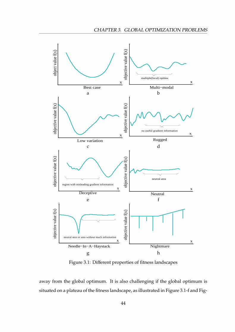
CHAPTER 3. GLOBAL OPTIMIZATION PROBLEMS
xBest case
obje
ct v
alue
f(x)
x
obje
ctiv
e va
lue
f(x)
Multi−modal
multiple(local) optima
a b
x
Low variation
obje
ctiv
e va
lue
f(x)
x
Rugged
obje
ctiv
e va
lue
f(x)
no useful gradient information
c d
xregion with misleading gradient informationob
ject
ive
valu
e f(
x)
Deceptivex
obje
ctiv
e va
lue
f(x)
Neutral
neutral area
e f
x
obje
ctiv
e va
lue
f(x)
Needle−In−A−Haystack
neutral area or area without much information
xNightmare
obje
ctiv
e va
lue
f(x)
g h
Figure 3.1: Different properties of fitness landscapes
away from the global optimum. It is also challenging if the global optimum is
situated on a plateau of the fitness landscape, as illustrated in Figure 3.1-f and Fig-
44

CHAPTER 3. GLOBAL OPTIMIZATION PROBLEMS
ure 3.1-g, because an optimizer can not find any gradient information to guide the
search. In addition, many other aspects also make the fitness landscape difficult
to optimize, e.g., noise, dynamism, rotation, shift, and dimensional linkage, etc.
In the following section, we introduce some global optimization benchmarks,
including un-rotated, shifted, rotated shifted as well as composition functions,
used in this thesis.
3.2 Test Functions
In this section, we chose 45 test functions, including traditional functions, tradi-
tional functions with noise, shifted functions, and rotated shifted functions, which
are widely used in the literature [43, 76, 136, 138] as well as the complex hybrid
composition functions proposed recently in [42, 106], to test an algorithm’s per-
formance. The details of these test functions are given in Table 3.1, Table 3.2, and
Table 3.3. The 45 functions are divided into six groups in terms of their properties:
traditional problems ( f1- f12) , noisy problems ( f19- f22), shifted problems ( f15- f18,
f31- f32, and f36- f38), rotated problems ( f23- f26), rotated shifted problems ( f27- f30,
f33- f35, and f39), and hybrid composition functions ( f13- f14 and f40- f45). Table 3.4
shows the parameter settings for some particular functions ( f3, f12- f14, f23- f30).
The detailed parameter setting for functions f31- f45 can be found in [106] with the
corresponding functions.
3.2.1 Traditional Test Problems
To test the performance of the proposed algorithms on standard test problems,
we selected 12 test functions. Five of them are unimodal problems, which are
considered easy to solve. They are the Sphere function ( f1), Rosenbrock function
( f8), Schwefel 2 22 ( f9), Schwefel 1 2 ( f10), and Schwefel 2 21 ( f11). The others in
45

CHAPTER 3. GLOBAL OPTIMIZATION PROBLEMS
Table 3.1: The test functions, where fmin is the minimum value of a function andS ∈ Rn
Name Test Function S fmin
Sphere f1(x) =∑n
i=1 x2i [−100, 100] 0
Rastrigin f2(x) =∑n
i=1 (x2i − 10 cos(2πxi) + 10) [-5.12, 5.12] 0
Noncont Rastrigin f3(x) =∑n
i=1 (y2i − 10 cos(2πyi) + 10) [-5.12, 5.12] 0
Weierstrass f4(x) =n∑
i=1(kmax∑k=0
[ak cos(2πbk(xi + 0.5))]) − nkmax∑k=0
[ak cos(πbk)], [-0.5,0.5] 0
a = 0.5, b = 3, kmax = 20
Griewank f5(x) = 14000∑n
i=1(xi − 100)2 −∏ni=1cos( xi−100√
i) + 1 [-600, 600] 0
Schwefel f6(x) = 418.9829 · n +∑ni=1 −xi sin (
√|xi|) [-500, 500] 0
Ackley f7(x) = −20 exp(−0.2√
1n∑n
i=1 x2i ) − exp( 1
n∑n
i=1 cos(2πxi)) + 20 + e [-32, 32] 0
Rosenbrock f8(x) =∑n
i=1 100(x2i+1 − xi)2 + (xi − 1)2) [-2.048, 2.048] 0
Schwefel 2 22 f9(x) =∑n
i=1 |xi| +∏n
i=1 |xi| [-10, 10] 0
Schwefel 1 2 f10(x) =∑n
i=1 (∑i
j=1 x j)2 [-100, 100] 0
Schwefel 2 21 f11(x) = maxni=1 |xi| [-100, 100] 0
Penalized 1 f12(x) = π30 {10 sin2 (πy1) +
∑n−1i=1 (yi − 1)2 · [1 + 10 sin2 (πyi+1)]+ [-50, 50] 0
(yn − 1)2} +∑ni=1 u(xi, 5, 100, 4), yi = 1 + (xi + 1)/4
H Com f13(x) =Hybrid Composition function (CF4) in [42] [-5, 5] 0
RH Com f14(x) =Hybrid Composition function (CF4) with rotation in [42] [-5, 5] 0
Table 3.2: Test functions of f15 to f30, where “O” represents the original problems,“N”,“S”, “R”, and “RS” represent the modified problems by adding noise, shifting,rotating, and combination of shifting and rotating, respectively.
O N S R RS O N S R RSSphere f1 f19 f18 f23 f27 Schwefel f6 f20 f15 f25 f28
Rastrigin f2 f22 f17 f24 f30 Ackley f7 f21 f16 f26 f29
this group are multi-modal problems where the number of local optima increases
exponentially with the number of dimensions. These problems appear to be
difficult to solve for many optimization algorithms. The Rastrigin function ( f2)
has a large number of local optima, which may easily trap algorithms into a
local optimum. Hence, to solve this problem, algorithms should maintain a large
diversity. The Noncontinuous Rastrigin function ( f3) is constructed based on the
Rastrigin function and has the same number of local optima as the continuous
Rastrigin function. The Weierstrass function ( f4) is continuous but differentiable
only on a set of points. The Griewank function ( f5) has linkages among variables,
which make it difficult to find the global optimum but the difficulty decreases
46

CHAPTER 3. GLOBAL OPTIMIZATION PROBLEMS
Table 3.3: Test functions of f31 to f45 chosen from [106]f Name&function number in [106] S fmin
f31 S Sphere CEC05(F1) [-100,100] -450f32 S Rastrigin CEC05(F9) [-5,5] -330f33 RS Rastrigin CEC05(F10) [-5,5] -330f34 RS Weierstrass CEC05(F11) [-0.5,0.5] 90f35 RS Ackley Bound CEC05(F8) [-32,32] -140f36 S Rosenbrock CEC05(F6) [-100,100] 390f37 S Schwefel 1 2 CEC05(F2) [-100,100] -450f38 S Schwefel 1 2 Noisy CEC05(F4) [-100,100] -450f39 RS Elliptic CEC05(F3) [-100,100] -450f40 Com CEC05(F15) [-5,5] 120f41 H Com CEC05(F16) [-5,5] 120f42 H Com Noisy CEC05(F17) [-5,5] 120f43 RH Com CEC05(F18) [-5,5] 10f44 RH Com NarrowBasin CEC05(F19) [-5,5] 10f45 RH Com Bound CEC05(F20) [-5,5] 10
when the number of dimensions increases [123]. The Ackley function ( f7) has
one narrow global optimum basin and many minor local optima. But it can be
easily solved as its local optima are shallow. The Schwefel function ( f6) is difficult
to solve due to its deep local optima being far from the global optimum. The
Penalized function 1 ( f12) is easy to solve as its local optima are shallow.
Table 3.4: Parameters settings for f3, f12, f13, f14, the rotated and rotated shiftedfunctions
f Parameter values
f3 yi =
{xi, |xi| < 1/2,round(2xi), |xi| ≥ 1/2
f12 u(x, a, k,m) =
k(x − a)m, x > a,0, −a ≤ x ≤ a,k(−x − a)m, x < −a.
m=10, M1−10( f13)=identity matrix, c1−10( f14)=2f13 g1−2 = Sphere function, g3−4=Rastrigin function, g5−6=Weierstrass functionf14 g7−8=Griewank function,g9−10=Ackley function
biask = 100(k − 1), k = 1, 2, . . . , 10f29 c=100
f23– f28, f30 c=2
3.2.2 Noisy Test Problems
In order to test an algorithm’s performance in noisy environments, the functions
f19 - f22 are modified from four traditional test functions ( f1, f6, f2, and f7) by adding
47

CHAPTER 3. GLOBAL OPTIMIZATION PROBLEMS
noise in each dimension by:
f (x) = g(x − 0.01 · orand)
where orand is a vector of uniformly distributed random numbers within (0, 1)
generated for each fitness evaluation.
3.2.3 Shifted Test Problems
In some problems, the global optimum has the same parameter value in all di-
mensions (e.g., the Rosenbrock function ( f8) has a global optimum of [1,1,...,1]).
In some other problems, the global optimum is always located in the origin (e.g.,
the Rastrigin function ( f2) has a global optimum at the origin [0,0,...0]). Due to
the simple properties of the global optimum in these types of test problems, some
researchers may develop algorithms that specifically exploit these properties. For
example, if the global optimal values of one dimension is found by the algorithm,
the values of all remaining dimensions can be easily obtained by copying the
found value to these dimensions. To avoid this bias, the shifted problems f15- f18
are extended from existing standard benchmark problems by shifting the global
optimum to a random position within the search range. The shifted functions
f31- f32 and f36- f38 were chosen from [106]. The functions with prefix of “S ” are
shifted problems in Table 3.2 and Table 3.3. The global optima of the problems in
this group were shifted by:
f (x) = g(x − orand)
where the new global optimum onew = orand + oold, where orand, oold, and onew are
the random position, the original global optimum, and the new global optimum,
respectively. orand is initialized once at the beginning of the run and keeps the
same for all the fitness evaluations during the whole run.
48

CHAPTER 3. GLOBAL OPTIMIZATION PROBLEMS
3.2.4 Rotated Shifted Test Problems
Some multi-modal functions in the first group are separable problems. This type of
problems have a special property: they can be solved by using D one-dimensional
search methods, like the ones used in some co-evolutionary algorithms. To avoid
this bias, we rotated and shifted some functions in the first group. The functions
with prefix of “RS ” are rotated shifted problems in Table 3.2 and Table 3.3. We
have eight rotated and shifted problems in this group, which are rotated and
shifted by the method used in [106]:
f (x) = g((x − orand) ∗M)
where M is a linear transformation matrix generated using:
M = P ∗N ∗Q
where P and Q are orthogonal matrices obtained by classical Gram-Schmidt
method, N is a diagonal matrix where the main diagonal entries are produced by:
nii = cui−min(u)
max(u)−min(u) ,u = U(1,D)
where D is the number of dimensions, U(1,D) is a random number uniformly
distributed in [1,D]; c=Cond(M) is the condition number of the matrix M, and
c is a constant which is set to different values as listed in Table 3.4 for the four
functions in this group.
3.2.5 Hybrid Composition Test Problems
In order to further test an algorithm’s performance on complex problems, eight
hybrid composition functions were chosen. The functions f13 and f14 were defined
49

CHAPTER 3. GLOBAL OPTIMIZATION PROBLEMS
in [42] and the other six ( f40- f45) listed in Table 3.3 were defined in [106]. Hybrid
composition functions are constructed using some basic benchmark functions to
create even more challenging problems with a randomly located global optimum
and several randomly located deep local optima.
The composition function can be described as:
f (x) =m∑
i=1
(wi · (g′i ((x − orandi)/λi ∗Mi) + biasi)) (3.3)
where f (x) is the composition function; gi(x) is i-th basic function used to construct
the composition function; m is the number of basic functions; Mi is the linear
transformation matrix for each gi(x); ooldi + orandi is the optimum of the changed
gi(x) caused by shifting the landscape. ooldi and orandi are the optima of the original
gi(x) without any change and a random position generated for the changed gi(x),
respectively. The value of ooldi is 0 for all the basic functions used in this group.
The weight value wi for each gi(x) is calculated as:
wi = exp(−sqrt(
∑nk=1 (xk − ok
i + okoldi
)2
2nσ2i
))
wi =
wi if wi = max(wi)
wi · (1 −max(wi)10) if wi , max(wi)
wi = wi/m∑
i=1
wi
where σi is the converge range factor of gi(x), whose default value is 1.0; λi is the
stretch factor for each gi(x), which is defined as:
λi = σi ·Xmax − Xmin
ximax − xi
min
50

CHAPTER 3. GLOBAL OPTIMIZATION PROBLEMS
where [Xmax,Xmin]n is the search range of f (x) and [ximax, xi
min]n is the search range
of gi(x).
In Eq. (3.3), g′i (x) = C · gi(x)/|gimax|, where C is a predefined constant, which is
set to 2000, and gimax is the estimated maximum value of gi(x), which is estimated
as:
gimax = gi(xmax ·Mi)
The details of functions f13 and f14 are given in Table 3.4. The only difference
between functions f13 and f14 is that f14 is rotated while f13 is not. This makes f14
more complex than f13. Although in [106] the authors proposed eleven hybrid
composition functions, we chose only six typical problems ( f40- f45) for testing
because the other functions also have similar properties and difficulty level as the
ones we selected.
It should be noticed that there are three pairs of functions in Table 3.2 and
Table 3.3 where each pair of functions have similar property. They are ( f17, f32),
( f18, f31), and ( f30, f33). For each pair, the differences are that the former chosen from
[106] have bias value but no in the later and the locations of the global optima
are also different. However, for convenient comparison, we still take the two
functions of each pair as different functions.
3.3 Performance Metrics
We test all algorithms over a certain number of independent runs on a specific
problem and then calculate the statistical results in different ways. In order
to show an algorithm’s performance in terms of different aspects, we use several
performance metrics, such as, the mean value, variance, and success rate. To com-
pare two different algorithms’ performance on a particular problem, we perform
a two-tailed T-test operation. To compare overall performances of algorithms on
51

CHAPTER 3. GLOBAL OPTIMIZATION PROBLEMS
all the 45 static problems, we calculate the winning ratio and equal ratio, which
are defined in the following section.
To evaluate an algorithm’s performance on static problems, we record the
mean value of the difference between the best result found by the algorithm and
the global optimum value over a certain number of runs (N) for each problem:
mean =1N
N∑k=1
( f (xk) − f (x∗))
where xk and x∗ represent the best solution found by the algorithm in the kth run
and the global optimum, respectively.
To compare two algorithms’ performance on the statistical level, the two-tailed
t-test with 58 degrees of freedom at a 0.05 level of significance was conducted
between two algorithms with N=30. The performance difference is significant
between two algorithms if the absolute value of the t-test result is greater than 2.0.
To compare two algorithms’ overall performance on the 45 problems, we define
a winning ratio of algorithm a against algorithm b (wr(a, b)) together with an equal
ratio (er(a, b)) as follows:
wr(a, b) =F∑
f=1
B f (a, b)/F∑
f=1
B f (b, a) (3.4)
er(a, b) =F∑
f=1
(1 − B f (a, b) − B f (b, a))/F (3.5)
where F=45 and if the performance of algorithm a is significantly better than
algorithm b on function f in terms of the t-test result, B f (a, b) returns 1; otherwise
B f (a, b) returns 0. From the two equations, we can see that the larger the winning
ratio and the smaller the equal ratio, the bigger the overall performance difference
between algorithm a and algorithm b.
52

CHAPTER 3. GLOBAL OPTIMIZATION PROBLEMS
Table 3.5: Accuracy level of the 45 problemsAccuracy level Function
1.0e-6 f1, f7, f9, f11, f12, f16, f18, f19, f21, f23
f26, f27, f29, f31, f35, f39
0.01 f2, f3, f4, f5, f6, f8, f10, f15, f17, f20, f22 , f24
f25, f28, f30, f32, f33, f34, f36, f37, f38
0.1 f13, f14, f40 , f41 , f42 , f43 , f44 , f45
Another performance metric is the success rate, which is to calculate the rate
of the number of successful runs over the total number of runs. A successful run
means an algorithm achieves the fixed accuracy level within a fixed number of
evaluations for a particular problem. The accuracy level for each test problem is
give in Table 3.5.
3.4 Summary
This chapter briefly discussed the difficulties for algorithms to solve global op-
timization problems. Some examples of how to modify traditional problems to
make them harder to solve, e.g., rotating and shifting the fitness landscape, adding
noise, and the composition method, are introduced. To evaluate and compare per-
formances of different algorithms investigated in this thesis, some performance
metrics are also defined in this chapter.
53

Chapter 4
Dynamic Optimization Problems
In recent years, there has been a growing interest in studying EAs for DOPs due
to its importance in real world applications since many real world optimization
problems are DOPs. Over the years, a number of dynamic problem generators
have been used in the literature to create dynamic test environments to compare
the performance of EAs. Generally speaking, they can be roughly divided into
two types.
For the first type, the environment is just switched between several stationary
problems or several states of a problem. For example, many researchers tested
their approaches on the dynamic knapsack problem where the weight capacity of
the knapsack changes over time, usually oscillating between two or more fixed
values [59, 81]. Cobb and Grefenstette [21] used a dynamic environment that
oscillates between two different fitness landscapes. For this type of generators, the
environmental dynamics is mainly characterized by the speed of change measured
in EA generations.
The second type of DOP generators construct dynamic environments by re-
shaping a predefined fitness landscape. For example, Branke [13] proposed the
MPB problem, which consists of a number of peaks in a multi-dimensional land-
scape, where the height, width, and position of each peak can be altered a little
54

CHAPTER 4. DYNAMIC OPTIMIZATION PROBLEMS
Figure 4.1: Dynamism in the fitness landscape
every time the environment changes. This function is capable of generating a
given number of peaks in a given number of dimensions that vary both spatially
(position and shape of a peak) and in terms of fitness. Morrison and De Jong [79]
also defined a dynamic problem generator that is similar to the MPB problem.
To evaluate an algorithm’s performance under different kinds of dynamisms, Li
and Yang proposed the GDBG benchmark [64, 68], which has seven different
environmental change types.
To understand how the fitness landscape changes over time, Figure 4.1 shows
four episodes in different time steps of the MPB problem [13]. It can be seen from
the figure, some elements are changing from time step t = 1 to time step t = 4.
The height, width, shape, location, and the number of peaks are changing over
time.
Change types are also variable. For example, in the GDBG [64, 68] system, it has
small step change, large step change, random change, chaotic change, recurrent
change, recurrent change with noise, and dimensional change. Therefore, all
55

CHAPTER 4. DYNAMIC OPTIMIZATION PROBLEMS
these dynamic characteristics require algorithms to quickly response and adapt
to the new environments, and make DOPs more complex and harder to optimize
than stationary problems.
In this chapter, three popular dynamic benchmarks are introduced to test an
algorithm’s performance in dynamic environments. They are the MPB problem
[13], the DF1 function generator [79], and the GDBG benchmark [64, 68].
4.1 The MPB Problem
The MPB problem proposed by Branke [13] has been widely used as dynamic
benchmark problems in the literature. Within the MPB problem, the optima can
be varied by three features, e.g., the location, height, and width of peaks. For the
D-dimensional landscape, the problem is defined as follows:
F(x, t) = maxi=1,...,p
Hi(t)
1 +Wi(t)∑D
j=1 (x j(t) − Xi j(t))2(4.1)
where Wi(t) and Hi(t) are the height and width of peak i at time t, respectively, and
Xi j(t) is the j-th element of the location of peak i at time t. The p independently
specified peaks are blended together by the max function. The position of each
peak is shifted in a random direction by a vector vi of a distance s (s is also called
the shift length, which determines the severity of the problem dynamics), and the
move of a single peak can be described as follows:
vi(t) =s∣∣∣r + vi(t − 1)
∣∣∣((1 − λ)r + λvi(t − 1)) (4.2)
where the shift vector vi(t) is a linear combination of a random vector r and the
previous shift vector vi(t−1) and is normalized to the shift length s. The correlated
parameter λ is set to 0, which implies that the peak movements are uncorrelated.
56

CHAPTER 4. DYNAMIC OPTIMIZATION PROBLEMS
Table 4.1: Default settings for the MPB problemParameter Value
p (number of peaks) 10change frequency 5000
height severity 7.0width severity 1.0
peak shape conebasic function noshift length s 1.0
number of dimensions D 5correlation coefficient λ 0
S [0, 100]H [30.0, 70.0]W [1, 12]I 50.0
More formally, a change of a single peak can be described as follows:
Hi(t) = Hi(t − 1) + height severity ∗ σ (4.3)
Wi(t) =Wi(t − 1) + width severity ∗ σ (4.4)
Xi(t) = Xi(t)(t − 1) + vi(t) (4.5)
where σ is a normally distributed random number with mean zero and variation
one.
The default settings and definition of the benchmark used in this thesis can be
found in Table 4.1. In Table 4.1, the change frequency is the number of evaluations
between two successive changes where the term “evaluation” means that an
individual is created and its fitness is evaluated, S denotes the range of allele
values, and I denotes the initial height for all peaks. The dynamism of changes
is described as follows. The height of peaks is shifted randomly in the range
H = [30, 70] and the width of peaks is shifted randomly in the range W = [1, 12].
57

CHAPTER 4. DYNAMIC OPTIMIZATION PROBLEMS
4.2 The DF1 Generator
The dynamic problem generator DF1, proposed by Morrison and De Jong [79],
is a kind of moving peaks benchmark generators. Within the DF1 generator, the
base landscape in the D-dimensional real space is defined as:
f (x) = maxi=1,...,p
Hi − Ri ×
√√√ D∑j=1
(x j − Xi j)2
(4.6)
where x = (x1, · · · , xD) is a point in the landscape, p specifies the number of peaks
(or cones), and each peak i is independently specified by its height Hi, its slope Ri,
and its center Xi = (Xi1, · · · ,XiD). The fitness at a point on the surface is assigned
the maximum height of all optima at that point; the optima with the greatest
height at a point is said to be visible at that point.
Just like the MPB problem [13], DF1 creates dynamic problems by changing
the features, i.e., the location, height, and slope of each peak independently. The
dynamics are controlled by the Logistics function given by:
∆t = A · ∆t−1 · (1 − ∆t−1) (4.7)
where A is a constant value in the range [1.0, 4.0] and ∆t is used as the step size
of changing a particular parameter (i.e., the location, height, or slope) of peaks at
iteration t after scaled by a scale factor s in order to reduce step sizes that may be
larger than intended for each step. The Logistics function allows a wide range of
dynamic performance by a simple change of the value of A, from simple constant
step sizes, to step sizes that alternate between two values, to step sizes that rotate
through several values, to completely chaotic step sizes. The default parameter
settings are shown in Table 4.2. More details on DF1 can be found in [79].
58

CHAPTER 4. DYNAMIC OPTIMIZATION PROBLEMS
Table 4.2: Parameter Settings for the DF1 FunctionParameter value
number of dimensions D 2A 1.2,3.3,3.99
number of peaks p 3change frequency U 6000
population size 60H [1.0,5.0]W [1.0,5.0]S [-1.0,1.0]
scale factor s 0.4
4.3 The GDBG System
The GDBG system proposed by Li and Yang [64] defines a DOP as below:
F = min f (x, ϕ, t) (4.8)
where f is the cost function, x is a feasible solution in the solution set, t is the
real-world time, and ϕ is the system control parameter(s). The GDBG system
constructs dynamic environments by changing the system control parameter(s).
It can be described as follows:
ϕ(t + 1) = ϕ(t) ⊕ ∆ϕ (4.9)
where ∆ϕ is a deviation from the current system control parameters. Then, the
new environment at the next moment t + 1 is obtained as follows:
f (x, ϕ, t + 1) = f (x, ϕ(t) ⊕ ∆ϕ, t) (4.10)
The GDBG system can be instantiated to construct DOPs in different space
domains, including binary, real, and combinatorial spaces. In this thesis, we use
59

CHAPTER 4. DYNAMIC OPTIMIZATION PROBLEMS
the real space instance to construct real-encoded DOPs as described in [68]. For
convenience, without special note, the term of “GDBG” benchmark refers to the
instances in real space in the GDBG system [64] in this thesis. In total, there are
seven basic test functions defined and each test function has seven change types,
which are small step change, large step change, random change, chaotic change,
recurrent change, recurrent change with noise, and dimensional change. The
seven change types are defined as follows:
T1 (small step): ∆ϕ = α · ∥ϕ∥ · r · ϕseverity
T2 (large step): ∆ϕ = ∥ϕ∥ · (α · sign(r) + (αmax − α) · r) · ϕseverity
T3 (random): ∆ϕ = N(0, 1) · ϕseverity
T4 (chaotic): ϕ(t + 1) = A · ϕ(t) · (1 − ϕ(t)/∥ϕ∥)
T5 (recurrent): ϕ(t + 1) = ϕmin + ∥ϕ∥(sin( 2πP t + φ) + 1)/2
T6 (recurrent with noise): ϕ(t + 1) = ϕmin + ∥ϕ∥(sin(2πP t + φ) + 1)/2 + N(0, 1) ·
noiseseverity
T7 (dimensional change): D(t + 1) = D(t) + f lag · ∆D
where ∥ϕ∥ is the range of ϕ, ϕseverity ∈ (0, 1) is the change severity of ϕ, ϕmin is
the minimum value of ϕ, noiseseverity ∈ (0, 1) is the noise severity in the recurrent
with noise change. α ∈ (0, 1) and αmax ∈ (0, 1) are constant values, which are set
to 0.04 and 0.1 in the GDBG system, respectively. The Logistics function is used
in the chaotic change type, where A is a positive constant in the range (1.0, 4.0).
If ϕ is a vector, the initial values of the items in ϕ should be different within ∥ϕ∥
in the chaotic change. P is the period of the recurrent change and the recurrent
change with noise, φ is the initial phase, r is a random number in (−1, 1), sign(x)
returns 1 when x is greater than 0, −1 when x is less than 0, or 0 otherwise. N(0, 1)
denotes a normally distributed one-dimensional random number with mean zero
60

CHAPTER 4. DYNAMIC OPTIMIZATION PROBLEMS
Table 4.3: Default settings for the GDBG benchmarkParameter Value
number of dimensions D fixed: 10; changing: [5-15]search range x ∈ [−5, 5]D
number of functions or peaks p 10change frequency U 10, 000 ×D fitness evaluations
number of changes K K = 60period P 12
severity of noisy noisyseverity = 0.8chaotic constant A 3.67
step severity α = 0.04maximum of α αmax = 0.1height range h ∈ [10, 100]initial height initial height = 50
severity of height change ϕ hseverity = 5.0sampling frequency s f 100 fitness evalutions
and standard deviation one. ∆D is a predefined constant, which is set to 1 by
default. If D(t) = Dmax, f lag = −1; if D(t) = Dmin, f lag = 1. Dmax and Dmin are the
maximum and minimum number of dimensions, respectively.
The seven basic test functions defined in [68] are the rotation peak function
with 10 peaks (F1 with p = 10), the rotation peak function with 50 peaks (F1 with
p = 50), the composition of Sphere’s functions (F2), the composition of Rastrigin’s
functions (F3), the composition of Griewank’s functions (F4), the composition of
Ackley’s functions (F5), and the hybrid composition function (F6). The parameters
of the seven problems are set the same as in [68]. The general parameter settings
are given in Table 4.3 and the detailed settings of F1 to F6 can be found from [68].
Generally speaking, the GDBG benchmark is much harder to locate and track
the global optima than the MPB and DF1 problems. Due to the huge number
of local optima and the higher number of dimensions of the GDBG benchmarks,
the complexity of some test functions (e.g., F2 - F6) is much higher than the MPB
and DF1 problems. For example, the visual comparison of the complexity of a
61

CHAPTER 4. DYNAMIC OPTIMIZATION PROBLEMS
One episode of the MPB problem One episode of the GDBG bechmark
Figure 4.2: Comparison of the MPB problem and the GDBG benchmark
fitness landscape created by the MPB problem and a fitness landscape created by
the GDBG benchmark can be found from Figure 4.2. Figure 4.2 clearly shows that
the fitness landscape of the GDBG benchmark is much rougher than that of the
MPB problem, and the number of local optima of the GDBG benchmark is also
far more than that of the MPB problem.
4.4 Performance Metrics
For different dynamic generators, different performance metrics are defined to
evaluate an algorithm’s performance. The details of these performance metrics
are described in the following sections. It should be noticed that the problems
used in dynamic environments are maximization problems that are different from
the global optimization problems used in this thesis.
4.4.1 Performance Metrics for the MPB Problem
The performance measure used for the MPB problem is the offline error, which is
defined as follows:
µ =1K
K∑k=1
(hk − fk), (4.11)
62

CHAPTER 4. DYNAMIC OPTIMIZATION PROBLEMS
where fk is the best solution obtained by an algorithm just before the k-th environ-
mental change, hk is the optimum value of the k-th environment, µ is the average
of all differences between hk and fk over the environmental changes, and K is the
total number of environments.
4.4.2 Performance Metrics for the DF1 Function
Two performance measure methods, as used in [84], are described for the DF1
problem. They are the global offline error (eg) and the average offline error (eavg).
The global offline error is defined as follows:
ek = 1 − fgk/hgk (4.12)
eg =1K
K∑k=1
ek (4.13)
where fgk and hgk are the best particle’s fitness and the height of the global op-
timum just before the k-th environmental change, and K is the total number of
environments.
In order to measure the ability of an algorithm to track multiple optima in
addition to the global optimum, the average of the best “local” errors since the
last environmental change over all visible peaks is calculated as follows:
eavgk =1|pk|
|pk |∑i=1
eik (4.14)
where eik is relative error of the best particle’s fitness on a visible peak i to the
height hik of peak i at the last generation of environment k, pk denotes those peaks
that are visible at the last generation of environment k, and |pk| is the number of
63

CHAPTER 4. DYNAMIC OPTIMIZATION PROBLEMS
n 10
(100) k+1 k
2
5
4
3
2
n 10
(100)
T 7 (10) T
1 (15)- - -T
6 (15)
F 2 (16)- - - F
6 (16) F
1 (20)
Performance(100)
m 10
(50) m 50
(50)
m 10
(50) m 50
(50)
T 7 (10) T
1 (15)- - -T
6 (15)
1
1
Figure 4.3: Overall performance marking measurement
such peaks. So, the average offline error eavg is calculated as:
eavg =1K
K∑k=1
eavgk (4.15)
When calculating eavgk , a particle is considered to be on an optimum if the
optimum is visible at the location of the particle. If no particle is on an optimum,
the local error for the optimum is the difference between the optimum’s height
and the fitness of the closest particle within the radius of the optimum’s apex. If
there is no particle on a peak, that peak is not included in the calculation of the
average local error.
4.4.3 Performance Metrics for the GDBG Benchmark
There are 49 test cases in total constructed from the seven test problems in the
GDBG benchmark. For an algorithm on each test case, the offline error (eo f f ) and
its standard variance (STD) are recorded, which are defined as in [68] as follows:
eo f f =1
R ∗ K
R∑r=1
K∑k=1
elastr,k (4.16)
64

CHAPTER 4. DYNAMIC OPTIMIZATION PROBLEMS
STD =
√∑Rr=1∑K
k=1 (elastr,k − eo f f )2
R ∗ K − 1(4.17)
where R and K are the total number of runs and the number of environmental
changes for each run, respectively, and elastr,k = | f (xbest(r, k))− f (x∗(r, k))|, where x∗(r, k)
is the global optimum of the k-th environment and xbest(r, k) is the position of the
best particle of the last generation of the k-th environment during the r-th run.
The overall performance of an algorithm on all 49 test cases is calculated using
the method proposed in [68], which is illustrated in Figure 4.3. In the figure, F1-F6
denote the six functions defined in the GDBG benchmark in [68], T1-T7 represent
the seven change types defined in Section 4.3, n10 means that the number of
dimensions is ten, and m10 and m50 denote that the number of peaks is 10 and 50,
respectively.
Each test case i is assigned a weight wi and the sum of weights of all the test
cases is 1.0. The mark obtained by an algorithm on test case i ∈ {1, . . . , 49} is
calculated by:
marki =wi
R ∗ K
R∑r=1
K∑k=1
(rlast
rk /(1 +
1S
S∑s=1
(1 − rsrk)))
(4.18)
where rlastrk is the relative ratio of the best particle fitness of the last generation to the
global optimum of the k-th environment, rsrk is the relative ratio of the best particle’s
fitness to the global optimum at the s-th sampling during the k-th environment
(initial population should be sampled), and S = U/s f is the total number of samples
for each environment. The relative ratio rsrk is defined by
rsrk =
f (xbest(r,k,s))
f (x∗(r,k)) , f = F1
f (x∗(r,k))f (xbest(r,k,s)) , f ∈ {F2,F3,F4, F5,F6}
(4.19)
where xbest(r, k, s) is the position of the best particle up to the s-th sample in the
65

CHAPTER 4. DYNAMIC OPTIMIZATION PROBLEMS
k-th environment during the r-th run.
The overall performance of an algorithm on all the test cases is then calculated
as follows:
per f ormance = 100 ×49∑i=1
marki (4.20)
4.5 Summary
This chapter introduced some basic methods of how to build the dynamic envi-
ronments to test the performance of EAs. Three popular benchmark generators,
including the MPB problem, the DF1 function, and the GDBG benchmark, are
described as well as their corresponding performance metrics.
66

Chapter 5
Self-learning Particle Swarm
Optimizer
So far, most PSO algorithms globally use a single learning pattern for all particles,
which means that all particles in a swarm use a same learning strategy. The
monotonic learning pattern may cause the lack of intelligence for a particular
particle, which makes it unable to deal with different complex situations. Actually,
due to different difficulties of different fitness landscapes, we need to develop
an intelligent system with different characteristics rather than a single learning
pattern to deal with different complex situations.
In order to bring more intelligence to the individual level, this chapter will
introduce a novel algorithm, called self-learning PSO (SLPSO). It will systemati-
cally describe the working mechanism of SLPSO in the following aspects. First, a
set of four learning strategies are introduced, which have different properties to
help particles deal with fitness landscapes with different properties. Second, an
adaptive learning framework is presented to enable each particle to adaptively
choose the best learning strategy according to its local fitness landscape. Third, in
order to extract useful information from improved particles, an information up-
67

CHAPTER 5. SELF-LEARNING PARTICLE SWARM OPTIMIZER
date method for the global best particle is described. Fourth, a monitoring method
is developed, which is able to accurately identify whether a general particle has
converged or not. Fifth, to increase diversity, a restart scheme is implemented to
create new swarms that are composed of restarted particles that are eliminated
from old swarms. Finally, a generalized parameter tuning method is introduced
for general problems. Also, multiple population methods are used to encourage
particles to explore unseen areas in the fitness landscape. How to systemically
organize these components together and make them work efficiently, will be dis-
cussed in detail in this chapter.
5.1 General Considerations
In this section, the open issues, which are challenges for EAs introduced in Sec-
tion 1.1 in Chapter 1, will be further discussed at a deep level in PSO, e.g., how
to tradeoff the performance between the gbest model and the lbest model, how
to avoid premature convergence, and what kind of intelligence a general particle
may need.
5.1.1 Tradeoff between the gbest and lbest Models
It is generally believed that the gbest model biases more toward exploitation, while
the lbest model focuses more on exploration. Although there are many improved
versions of PSO, the question of how to balance the performance of the gbest and
lbest models is still an important open issue, especially for multi-modal problems.
In the gbest model, all particles’ social behavior is strictly constrained by learn-
ing information from the gbest particle. The gbest particle is more attractive than
particles’ personal pbest positions because of the higher fitness of the global best
particle. Therefore, particles are easily attracted by the gbest particle and quickly
68

CHAPTER 5. SELF-LEARNING PARTICLE SWARM OPTIMIZER
converge to the region around the gbest particle even though that region does not
contain the global optimum. In the gbest model, once the whole swarm converges
to a local optimum, all particles will lose the capability of jumping out of the basin
of attraction of that local optimum since their velocity has reduced to zero.
In the lbest model, particles do not learn from the gbest particle of the whole
swarm but from the best particle of their neighborhood. Because of that, particles
that do not belong to the neighborhood of the gbest particle will not communicate
with the gbest particle. As a result, in the lbest model, particles are not easily
trapped in the area around the gbest particle. However, the trade-off is that the
convergence speed may be slower compared with the gbest model.
5.1.2 Premature Convergence
Another important issue is how to avoid premature convergence for EAs. Con-
vergence is one of the key performance metrics of EAs. Generally speaking, if
a swarm of particles converges to a point in the search space, it means that the
evolutionary process comes to an end. All individuals become inactive since they
have lost the search capability. According to the theory of self-organization [80],
if the system is going to be in an equilibrium, the evolution process will be stag-
nated. However, converging to a global optimum is not guaranteed for EAs. So,
we need to maintain the social diversity of swarm to keep on the evolutionary
process.
5.1.3 Individual Level of Intelligence
In order to achieve a good performance, a PSO algorithm needs to balance its
search between the lbest and gbest models. However, this is not an easy task. If we
let each particle simultaneously learn from both pbest and gbest to update itself, the
algorithm may suffer from the disadvantages of both models. One solution might
69

CHAPTER 5. SELF-LEARNING PARTICLE SWARM OPTIMIZER
be to implement the cognition component and the social component separately.
In this way, each particle can focus on exploitation by learning from its individual
pbest position or focus on convergence by learning from the gbest particle. The idea
enables particles of different locations in the fitness landscape to carry out local
search or global search, or vice versa, in different evolutionary stages. Different
particles can play different roles (exploitation or convergence) during the search
progress, and even the same particle can play different roles during the search
progress. Thanks to this flexibility, the probability of avoiding PSO from being
trapped in the basins of attraction of local optima may be increased. However,
there is a difficulty in implementing this idea: the appropriate moment for a
particle to learn from gbest or pbest is very hard to know.
To implement the idea above that allows particles to carry out different types
of search (local or global) at different evolutionary stages, we need an adaptive
method to automatically choose one type of search strategies. The method is
adaptive, i.e., it enables particles to adaptively switch from learning from global
information to learning from local information, and vice versa. Thanks to this
adaptive property, we can overcome the aforementioned difficulty of identifying
the appropriate learning stage for each particle. That is, which learning strategy
and when to apply that strategy are determined by the property of the local fitness
landscape where a particle is. The adaptive method will be further described later
in Section 5.3.
5.1.4 Maintaining Diversity by Intelligence
Maintaining diversity is an important method to prevent a population from be-
ing trapped in local optima. There are several methods to maintain population
diversity, e.g., maintaining diversity through the whole run, multi-population
methods, restart methods, etc. The restart method is simple and easy to imple-
70

CHAPTER 5. SELF-LEARNING PARTICLE SWARM OPTIMIZER
ment. However, to effectively use this technique, several open issues should be
addressed. For example, how to restart particles, and when to perform the restart
operation.
Maintaining the social diversity of a swarm can be achieved by refreshing the
inactive particles (converged particles). That is, we restart a particle if it converges
to a point in the search space. How to check the converged status of a particle and
how to introduce fresh particles will also be described in the following sections.
How to avoid explored areas in the fitness landscape is a challenging ques-
tion. Actually, maintaining diversity is a kind of idea that attempts to encourage
particles to explore new areas. However, little or no attempt has been made to
prevent particles from searching the areas that have been explored. To attempt to
achieve this goal, first we need to give an answer to the question of which regions
should be memorized by a particular particle. Second, we need to determine how
to prevent particles from searching the areas covered by the memorized regions.
These two issues will be discussed in the following sections in this chapter.
5.2 Learning Strategies in SLPSO
Inspired by the idea of division of labor, we can assign to particles different
roles, e.g., converging to the global best particle, exploitation of its personal best
position, exploring new promising areas, or jumping out of local optima. Which
role a particular particle should play is determined by the local fitness landscape
where it is. To assign to a particular particle individual level of intelligence, we
need to consider the possible situations of the local fitness landscape.
Take Figure 5.1 as an example, which shows the fitness landscape of a compo-
sition function with ten components, labeled by 1, 2, 3 . . . 10, respectively, in two
dimensions. The best learning strategy for particles in the sub-regions covered
by components 1, 2, 3, 4, and 10 may be to learn from their own personal best
71

CHAPTER 5. SELF-LEARNING PARTICLE SWARM OPTIMIZER
Figure 5.1: The fitness landscape of a composition function with ten componentsin two dimensions
positions since these components are relatively far away from each other and the
shape of them is similar to the unimodal Sphere function. While, for particles in
the sub-areas covered by components 5, 6, 7, 8, and 9, the best choice might be
to learn from their neighbor, because these components are close to each other
and they sit on several near ridges in the fitness landscape. The third case is
when a particle converges to a local optimum, the jumping out strategy might
help it escape from that local optimum. Another common case is when a particle
stands on a slope, the best strategy may be to learn from its own pbest position
or the particles with better fitness on the same slope. From Figure 5.1, we can
conclude that which learning strategy a particle should use depends on its local
fitness landscape. Therefore, we need to develop different learning strategies for
particles in different situations.
Based on the above idea, we define four learning strategies and corresponding
learning operators used in SLPSO. In SLPSO, the learning information for each
particle comes from four sources: the archive of the gbest particle (abest), its
individual pbest position, the pbest position of a random particle (pbestrand) whose
pbest is better than its own pbest, and a random position prand nearby. The four
learning strategies play the roles of convergence, exploitation, exploration, and
jumping out of the basins of attraction of local optima, respectively.
72

CHAPTER 5. SELF-LEARNING PARTICLE SWARM OPTIMIZER
The four learning strategies enable each particle to independently deal with
different situations. For each particle k, the learning equations corresponding to
the four learning operators respectively are given as follows:
Operator a: learning from its pbest position
exploitation : vdk = ωvd
k + η · rdk · (pbestd
k − xdk) (5.1)
Operator b: learning from a random position nearby
jumping out : xdk = xd
k + vdavg ·N(0, 1) (5.2)
Operator c: learning from the pbest of a random particle
exploration : vdk = ωvd
k + η · rdk · (pbestd
rand − xdk) (5.3)
Operator d: learning from the abest position
convergence : vdk = ωvd
k + η · rdk · (abestd − xd
k) (5.4)
where pbestrand is the pbest of a random particle, which is better than pbestk; the
jumping step vdavg is the average velocity of all particles in the d-th dimension,
which is calculated by vdavg =
∑Nk=1 |vd
k |/N, where N is the population size; N(0, 1)
is a random number generated from the normal distribution with mean 0 and
variance 1; the abest position is used to store the best position found by SLPSO so
far.
It should be noted that different from the standard PSO (SPSO), in SLPSO
a bias selection scheme is added into the operator of learning from the pbestrand
position. That is, a particle only learns from a pbestrand position that is better than
its own historical best position pbest. Due to this scheme, more resources are given
73

CHAPTER 5. SELF-LEARNING PARTICLE SWARM OPTIMIZER
Algorithm 5.1 Update(operator i, particle k, f es)1: if i = a then2: Update the velocity and position of particle k using operator a and Eq. (2.2);3: else if i = b then4: Update the position of particle k using operator b;5: else if i = c then6: Choose a random particle j that is not particle k;7: if f (xpbest j) < f (xpbestk) then8: Update the velocity and position of particle k using operator c and Eq. (2.2);9: else
10: Update the velocity and position of particle j using operator c and Eq. (2.2);11: end if12: else13: Update the velocity and position of particle k using operator d and Eq. (2.2);14: end if15: f es++;
where f es is the current number of fitness evaluations.
to the badly performing particles to improve the whole swarm. The procedure is
described in Algorithm 5.1.
It should also be noticed that the abest position in Eq. (5.4) is different from the
gbest particle of the whole swarm. Although it is the same position as the gbest
particle in the initial population, it will be updated by Algorithm 5.2 (it will be
explained later in Section 5.4) and gets better than the gbest particle. Different from
the ALPSO algorithm in [70], all particles in SLPSO, including the gbest particle,
learn from the abest position.
The four learning objectives of a particle in SLPSO can be visualized in Fig-
ure 5.2, where “psel f ” is a particle’s current position, “xrand” is generated within a
circle area with a radius of the mutation step (vavg), pbest rand is the pbest position
of a random particle, and abest is the archive of the gbest particle. The position
and velocity update framework in SLPSO is shown in Algorithm 5.1.
The first learning operator - learning from a particle’s own pbest position,
allows the particle to fully search in the area around its historical best position.
Such kind of exploitation helps a particle to find a better position much easier
74

CHAPTER 5. SELF-LEARNING PARTICLE SWARM OPTIMIZER
abestVelocity
pbest
pself
y
x
avgv
xrand
pbest_rand
Figure 5.2: The four Learning objectives of a particle in SLPSO
than it would do by searching in a region that is far away from its pbest position.
The second operator - learning from a random position nearby, is useful in the
case that a particle that already has converged to a local optimum but there is a
more promising region nearby which has not been explored by any particle. The
operator b will give particles a probability to jump to that promising region.
The third operator - communicating with a random neighbor, enables particles
to explore the non-searched areas with a higher probability than learning from its
nearest neighbor used in [70]. From the learning equation of Eq. (5.3), learning
from different particles can actually alter the velocity as the distance is differ-
ent from different random particles in two successive iterations. Therefore, this
learning strategy is able to maintain the social diversity of a swarm in a certain
level.
The fourth learning operator - learning from the abest position, focuses on
increasing the convergence speed, which is important for global optimization
algorithms. Like the gbest model, the information of the abest position is also
shared by all other particles of the whole swarm in SLPSO. Learning from the
abest position allows all other particles to quickly converge to the location of abest.
In SLPSO, the four learning options enable each particle to move to a promising
position with a higher probability than the original PSO. The choice of which
75

CHAPTER 5. SELF-LEARNING PARTICLE SWARM OPTIMIZER
learning option is the most suitable for a particular particle would depend on the
local fitness landscape where it is. However, it is assumed that we cannot know
how the fitness landscape looks like even though we have a priori knowledge
of the fitness landscape. Instead, each particle should detect the shape of the
local fitness landscape where it is currently in by itself. To implement the idea of
adaptively detecting the shape of the local fitness landscape, we use the method
proposed in [65] with some simplification, which enables a particle to choose the
most suitable operator automatically. The simplified method is described in the
following section.
5.3 The Adaptive Learning Mechanism
As analyzed above, the best learning strategy for a particular particle is deter-
mined by its local fitness landscape, so the optimal strategy for that particle may
change with the change of its position during the evolutionary process. In this
section, we will achieve two objectives: one is to provide a solution to how to
choose the optimal learning strategy, and the other is to adapt this learning mecha-
nism to the environmental change for a particular particle during the evolutionary
process.
5.3.1 Ideas of Operator Adaptation
The four learning operators in SLPSO represent four different population topolo-
gies, which in turn allow particles to have four different communication struc-
tures. Each population structure determines a particle’s neighborhood and the
way it communicates with the neighborhood. By adaptively adjusting the pop-
ulation topology, we can adaptively adjust the way particles interact with each
other and hence can make the PSO algorithm perform better in different situa-
76

CHAPTER 5. SELF-LEARNING PARTICLE SWARM OPTIMIZER
tions. However, currently there is very little research on adaptation of population
topologies. The most common adaptation methods in PSO are addition or re-
moval of particles [20] and parameters tuning [92, 98, 100, 138].
The task of selecting operators from a set of alternatives has been comprehen-
sively studied in EAs [27, 33, 102] and many techniques have been proposed to
solve this problem [23, 101, 109, 110]. Inspired by the idea of probability match-
ing [109], we introduce an adaptive framework using the aforementioned four
learning operators, each of which is assigned with a selection ratio. This adaptive
framework is an extension of the work we have done in [65]. Different from the
work in [65], which only implemented the adaptive scheme at a population level,
we will extend the adaptive scheme to the individual level and make it simpler
than the version in [70]. The adaptive framework is based on the assumption that
the most successful operator used in recent past iterations may be also successful
in the future several iterations. The selection ratio of each operator is equally ini-
tialized to 1/4 for each particle and is adaptively updated according to its relative
performance.
For each particle, one of the four learning operators is selected according to
their selection ratios. The operator that results in a higher relative performance,
which is evaluated by a combination of the offspring fitness, current success ratio,
and previous selection ratio, will have its selection ratio increased. Gradually, the
most suitable operator will be chosen automatically and control the leaning be-
havior of each particle in different local fitness landscapes during the evolutionary
progress.
5.3.2 Selection Ratio Update
The update method of the selection ratios of the four operators is also modified
compared with [70]. The operators’ selection ratios for a particle are updated only
77

CHAPTER 5. SELF-LEARNING PARTICLE SWARM OPTIMIZER
if it does not improve for U f successive iterations, where U f is called the updating
frequency. During the updating period for each particle, the progress value and
the reward value of operator i are calculated as follows.
The progress value pki (t) of operator i for particle k at iteration t is defined as:
pki (t) =
| f (xk(t)) − f (xk(t − 1)) |, if operator i is chosen
by xk(t) and xk(t) is better than xk(t − 1)
0, otherwise
(5.5)
The reward value rki (t) has three components, which are the normalized progress
value, the success rate, and the previous selection ratio. It is defined by:
rki (t) =
pki (t)∑M
j=1 pkj(t)α +
gki
Gki
(1 − α) + cki s
ki (t) (5.6)
where gki is the counter that records the number of successful learning times of
particle k, in which its child is fitter than particle k by applying operator i since
the last selection ratio update; Gki is the total number of iterations where operator
i is selected by particle k since the last selection ratio update;gk
i
Gki
is the success
ratio of operator i for particle k; α is a random weight between 0.0 and 1.0; M is
the number of operators; cki is a penalty factor for operator i of particle k, which is
defined as follows:
cki =
0.9, if gki = 0 and sk
i (t) = maxMj=1 (sk
j(t))
1, otherwise(5.7)
and ski (t) is the selection ratio of operator i for particle k at the current iteration.
Different from the reward calculation in Eq.(2.20) in [65], we removed the
exponential operation in Eq.(5.6) for simplicity. By removing the exponential
operation, here, the three components in Eq.(5.6) have roughly equal importance
to calculate the reward.
78

CHAPTER 5. SELF-LEARNING PARTICLE SWARM OPTIMIZER
By introducing the penalty factor in Eq. (5.6), the optimal learning strategy
is able to adapt to the environmental change for a particular particle during the
evolution process. As we know, when a particle moves to a new location in the
search space, the local fitness landscape around may also change. If the property
of the new local fitness landscape is quite different from the property of the
previous one where it moves from, it means the old optimal learning strategy
may not work any more in the new local fitness landscape. Therefore, it needs to
re-select a new optimal learning strategy. This can be achieved by punishing the
old optimal learning strategy like in Eq. (5.6).
Based on the above definitions, the selection ratio of operator i for particle k in
the next iteration t + 1 is updated according to the following equation:
ski (t + 1) =
rki (t)∑M
j=1 rkj(t)
(1 −M ∗ γ) + γ (5.8)
where γ is the minimum selection ratio for each operator, which is set to 0.01.
5.3.3 Working Mechanism
According to the above definitions, we know that there is usually one operator
that has the highest selection ratio with each particle. This operator must be the
most successful one compared with the other operators at the current moment.
However, when a particle converges or moves to a new local sub-region whose
property is different from the previous one, this most successful operator may
no longer bring any benefit to the particle. When this case happens, according
to the punishing mechanism in Eq. (5.7), the selection ratio of that operator will
decrease, while the selection ratios of the other operators will increase. So, a new
most suitable operator will be adaptively selected based on its relatively better
performance and the outdated operator will lose its domination automatically.
79

CHAPTER 5. SELF-LEARNING PARTICLE SWARM OPTIMIZER
This is how the adaptive mechanism works. Based on the analysis of the adap-
tive working mechanism, we can see that SLPSO is able to choose the optimal
learning strategy and is also able to adapt to the environmental change for each
independent particle. This kind of individual level of intelligence extends the
scale of problems that can be effectively solved by EAs.
In addition, it should be noticed that the selection ratios of the four operators
are updated at the same time and not updated every iteration. Instead of counting
the number of successive iterations for U f as in [70], we just record the number
of successive unsuccessful learning times (mk, see Algorithm 5.6 in Section 5.8).
If the value of the counter mk for particle k does not reach the maximal value of
U f and particle k is improved by any operator, the value of mk will be reset to 0.
This method reduces the risk of punishing the best operator due to its temporally
bad performance in a short period. After the selection ratios of the four learning
operators are updated, all the parameters of each operator, including the progress
value, the reward value, and the success ratio, is reset to 0, except the selection
ratio. The optimal value of U f depends on specific problems. If the value of
U f is too large, the algorithm may suffer from learning outdated information.
On the other hand, if the value of U f is too small, the algorithm may not have
enough knowledge to estimate the optimal selection ratio properly. How to set
this parameter for a general problem will be explained later in Section 5.7.
5.4 Information Update for the abest Position
In most PSO algorithms, the gbest particle is updated only when a better position
than the current gbest particle is found. Once it is updated, the information of
all dimensions of the gbest particle is replaced with that of the better position.
This updating mechanism has one disadvantage: promising information may not
always be preserved. For example, even though a particle has promising informa-
80

CHAPTER 5. SELF-LEARNING PARTICLE SWARM OPTIMIZER
tion in a particular dimension, that information would still be lost if the particle
has a lower fitness due to unpromising information from other dimensions. This
problem, called “two step forward, one step back” in [115], has two opposite
aspects to be considered regarding particles getting better or worse. Take the
separable Sphere function as an example. For particles getting improvement, one
aspect is that improvement of some dimensions on the gene level (the values of
corresponding dimensions move closer to the origin) brings the improvement on
the whole individual level. The other opposite aspect is that some dimensions
get worse (the values of corresponding dimensions move away from the origin)
although the whole individual gets better. Vice versa for the case of particles
getting worse.
Whether a particle get better or worse depends on whether the benefit from
the improvement dimensions is larger or less than the deterioration from the
worsen dimensions. This is also a common phenomenon in most evolutionary
algorithms. However, it is very difficult to find out which dimensions get better or
worse. This is because, firstly there may be inter-relationships among dimensions
and secondly the change of the objective function values may be not linearly
related to the change of the decision space.
Although it is difficult to find out which dimensions get better, we can mon-
itor the improved particles to attempt to extract improvement information from
certain dimensions. If a particle gets better over time, there may be the case that
the particle has some useful information in some certain dimensions even though
it has a relatively low fitness value. In that case, other particles should learn that
useful information. In SLPSO, the abest position learns the useful information
from the dimensions of particles which show improvement over time. Once the
promising information is extracted from the improved dimensions of a particle,
the information of corresponding dimensions of the abest position is updated.
81

CHAPTER 5. SELF-LEARNING PARTICLE SWARM OPTIMIZER
However, it is difficult to effectively implement this idea. For example, in order
to check the information of which dimension of an improved particle is useful for
the abest position, we have to check all the dimensions of that improved particle.
That is because it is very difficult to know the information of which dimension or
what combination of dimensions of the improved particle is useful for the abest
position.
Although we do not know which dimensions or what combination of dimen-
sions is useful for the abest position, we can assign a learning probability (Pl) of
each dimension for the abest position to learn from the improved particle. In-
troducing the learning probability has two advantages: firstly the algorithm will
save a lot of computational resources and secondly the algorithm can reduce the
probability of learning potentially un-useful information for the abest position
even if it also reduce the probability of learning useful information. That is, the
algorithm can utilize the saved computational resources to further explore the
search space. Intuitively, the benefit from the use of the saved computational
resources may compensate the loss of reducing the probability of learning useful
information. This is because, for many cases, the information of an improved
particle may be not useful for the abest position as they distribute in different
sub-regions of the search space. This means that assigning a learning probability
may not affect too much the performance of SLPSO. Keep in mind, although the
abest position gets better after a successful learning from an improved particle,
some dimensions of the abest position may get worse. If this case happens, the
abest position will learn potential bad information from improved particles, and
the performance of SLPSO will be seriously affected. The evidence can be seen
from the experimental results in the section of parameter sensitivity analysis in
Chapter 7. Algorithm 5.2 describes the update framework of the abest position.
82

CHAPTER 5. SELF-LEARNING PARTICLE SWARM OPTIMIZER
Algorithm 5.2 UpdateAbest(particle k, f es)1: for each dimension d of abest do2: if rand() < Pk
l then3: xt abest := xabest;4: xt abest[d] := xk[d];5: Evaluate xt abest;6: f es++;7: if f (xt abest) < f (xabest) then8: xabest[d] := xt abest[d];9: end if
10: end if11: end for
where Pkl is the learning probability for the abest position to learn from particle k.
5.5 Monitoring Particles’ Status
In this section, we will answer some open issues regarding the premature con-
vergence problem, e.g., how to identify a converged particle, when to perform
re-initialization operation, and which particles need to be restarted.
5.5.1 Population Re-initialization
Generally speaking, re-initialization is a common method to increase population
diversity in EAs. However, there are some open issues while using this method,
e.g., how to protect the re-initialized individuals from being eliminated since they
usually have very bad fitness. When to perform re-initialization is also an open
issue. Although the former issue does not exist in PSO since there is no selection
operation, we still have the later problem.
There are several ways to check when to perform re-initialization. The first
method is to check the population diversity by a given definition. If the population
diversity is less than a threshold, we perform re-initialization for some random
individuals or the whole population. The second is to monitor the global best in-
dividual. If it does not improve for a certain number of iterations, re-initialization
can be launched. For PSO algorithms, we can monitor a particle’s velocity. If the
83

CHAPTER 5. SELF-LEARNING PARTICLE SWARM OPTIMIZER
velocity’s magnitude of a particle reaches a threshold value, we can re-initialize
that particle. Whichever method we use, we have to define a threshold value to
perform this operation. However, it is very difficult to get an optimal threshold
value for a particular problem. In addition, the threshold values for different
problems probably are different because they are problem dependent.
The common problem of the above approaches is that they cannot examine
whether an individual is in the stage of evolution or in the stage of conver-
gence. If we can judge particles’ status (evolution or convergence), we will know
when to perform re-initialization. Consequently, the above problems of using
re-initialization methods will also be avoided. In order to monitor a particle’s
status, we introduce a method to check whether a particle is in the convergence
status or not.
5.5.2 Monitoring Particles’ Status
In SLPSO, there is a mechanism of monitoring the performance of the four learning
operators. The approach is to monitor the selection ratios of the four learning
operators. Once a particle converges to a local optimum, none of the four operators
can help it jump out of that local optimum. Due to the punishment mechanism,
their selection ratios will go back to the initial stage where they would have similar
equal values of 1/4. Hence, we can use this information to examine whether a
particle is converged or not. By using this approach, we can easily avoid the
above problems discussed regarding re-initialization.
To achieve this goal, in addition to calculate the common selection ratios de-
fined in Section 5.3, we need to create a monitoring selection ratio for each learning
operator. In SLPSO, every operation related to the update of the monitoring selec-
tion ratios is the same as described in Section 5.3 to update the common selection
ratios except calculating the progress value p′ki (t) of operator i for particle k at
84

CHAPTER 5. SELF-LEARNING PARTICLE SWARM OPTIMIZER
iteration t, which is defined as:
p′ki (t) =
| f (xk(t)) − f (xpbest
k ) |, if operator i is chosen by
xk and xk is better than xpbestk
0, otherwise,
(5.9)
To distinguish the definitions related to updating monitoring and common
selection ratios in SLPSO, we put a prime symbol after each definition defined
in Section 5.3, e.g., p′ki (t) and pki (t) represent the monitoring progress value and
common progress value of operator i for particle k at iteration t, respectively.
And the four learning operators referred to by the two different terms are called
common and monitoring operators in the following contents in this thesis.
The reason of introducing the monitoring selection ratios is that the common
selection ratios may not be able to monitor a particle’s status as a small fluctu-
ation of the psel f ’s fitness value will cause a large disturbance of the values of
the common selection ratios and this disturbance may affect SLPSO to correctly
judge a particle’s evolutionary status. However, the disturbance will not happen
for the monitoring operators since the pbest’s fitness value of a particle never
increases before re-initialization taking place during the evolution process. The
corresponding evidence can be seen in the experimental study in Section 7.2.1 in
Chapter 7.
In SLPSO, the common selection ratios and the monitoring selection ratios
are updated at the same time and once they are updated, all the component
parameters are reset to the initial states: progress values, reward values, success
ratios are set to 0. The re-initialization of a particle is performed only if the
variance of its monitoring selection ratios is less than a constant value of 0.05.
85

CHAPTER 5. SELF-LEARNING PARTICLE SWARM OPTIMIZER
5.6 Controlling the Number of Particles That Learn
from the abest Position
Learning from the abest position is used to accelerate the population convergence.
It has the similar property as the PSO with gbest model. As a result, for the
particles close to the abest position, the attraction to the abest position is too strong
to give opportunity to the other three learning operators. In order to make full use
of the adaptive learning mechanism, we need to control the number of particles
that learn to the abest position. There are two reasons to do so.
First, the optimal number of particles that learn from the abest position is de-
termined by the property of the problem to be solved. For example, to effectively
solve the unimodal function, e.g., the Sphere function, we need to allow all parti-
cles to learn from the abest position so that all particles can quickly converge to the
global optimum. On the contrary, for some multi-modal problems, we should al-
low most particles to do local search rather than to learn from the abest position so
that they will have a higher probability to find the global optimum. The evidence
can be seen from the experimental results in the section of parameter sensitivity
analysis in Section 7.2.3 of Chapter 7.
Second, it is not fair for the other three operators to compete with the conver-
gence operator, because all the other three operators contribute to the convergence
operator. In other words, when a particle gets improvement through whichever
of the other three operators, the convergence operator also gets benefit through
direct or indirect ways: the direct way is that the improved particle becomes the
new abest position, so that the abest position can be directly updated; the indirect
way is that to extract useful information from improved particles. If the abest
position succeeds, it will also indirectly get benefit.
Based on the above analysis, we need to control the number of particles that use
86

CHAPTER 5. SELF-LEARNING PARTICLE SWARM OPTIMIZER
the convergence operator. However, it is hard to know which particles are suitable
to use the convergence operator. To solve this problem, we randomly select a
certain number of particles to use the convergence operator every iteration. To
implement this idea, we need to update some information of the particles that are
switched to use or not to use the convergence operator in two successive iterations.
The information needed to be updated includes progress values, reward values,
success ratios, and selection ratios.
If the switch happens, there are two cases for updating the related information.
The first case is that particles use the convergence operator in previous iteration
but do not in current iteration, and the second case is opposite to the first one. In
the first case, for both common and monitoring operators, we need to remove the
learning source of the abest position, and then normalize the selection ratios of the
other three operators according to their current values and the other information
of the three operators is kept the same. For the second case, we need to process
the common and monitoring operators through different means. For the com-
mon operators, all the related information is reset to the initial states: progress
values, reward values, and success ratios are set to 0 and selection ratios are set
to 1/4 for the four common operators. While for the monitoring operators, the
related information of the convergence operator is set to the initial states and the
information of the other three operators keeps the same as the previous iteration
except the selection ratios are re-normalized based on their current values. The
update description can be seen in Algorithm 5.3.
5.7 Parameters Tuning in SLPSO
There are three key parameters in SLPSO: the update frequency (U f ), the learning
probability (Pl), and the number of particles that learn to the abest position (M).
The values of the three parameters significantly affect the performance of SLPSO
87

CHAPTER 5. SELF-LEARNING PARTICLE SWARM OPTIMIZER
Algorithm 5.3 UpdateLearningOpt(particle k)1: if CFk!=true & PFk=true then2: sum:=
∑3j=1 sk
j ; sum′:=∑3
j=1 s′kj ;3: for j=1 to 3 do4: sk
j :=skj/sum; s′kj :=s′kj /sum′;
5: end for6: sk
4:=0;s′k4 :=0;7: end if8: if CFk=true & PFk!=true then9: for j=1 to 4 do
10: pkj :=0;gk
j :=0; Gkj :=0; sk
j :=1/411: end for12: sum′:=
∑3j=1 s′kj ;
13: for j=1 to 3 do14: s′kj = s′kj /sum′∗(1-1/4);15: end for16: p′k4 :=0;g′k4 :=0; G′k4 :=0; s′k4 :=1/4;17: end if
where CFk and PFk are used to record whether particle k uses the convergence operator or not at current and previous
iteration, respectively.
in most problems tested in this thesis. To achieve the best performance for SLPSO,
different optimal values of U f , Pl, and M are needed in different problems. This
can be seen from the experimental results regarding the parameter sensitivity
analysis in Section 7.2.3 in Chapter 7. For example, a small value of Pl helps
SLPSO to achieve the best performance in the Sphere function while the same
value negatively affects the performance of SLPSO in the Rastrigin problem. In
order to achieve the best performance in different problems without manually
tuning the parameters, this section suggests an approach to adjusting the values
of the three parameters for a general problem.
5.7.1 Setting the Update Frequency
First, we present a general solution to set up the values of the update frequency
(U f ) for SLPSO in all problems. Based on our previous work in [70], the optimal
values of U f mainly distribute from 1 and 10 in most problems tested in [70]. This
88

CHAPTER 5. SELF-LEARNING PARTICLE SWARM OPTIMIZER
information is very useful for SLPSO to set up U f for a particular problem even
if we cannot know the optimal value of U f for that problem. In order to use this
information, we assign to each particle a different value of U f instead of using a
same value of U f for all particles. The value of U f for particle k is defined by the
following empirical equation.
Ukf = max(10 ∗ exp(−(1.6 · k/N)4), 1) (5.10)
where N is the population size and Ukf is the update frequency of particle k. By
using this scheme, the values of U f of all particles distribute from 1 to 10. As a
result, it is possible that some particles might be able to achieve the optimal value
of U f for different problems.
5.7.2 Setting the Learning Probability
For the learning probability (Pl) parameter, we use the same method as used for
setting up the update frequency, which is described as follows:
Pkl = max(1 − exp(−(1.6 · k/N)4), 0.05) (5.11)
where N is the population size. Figure 5.3 describes the initial learning probability
of each particle in a swarm with the population size of 10. From Figure 5.3, we
can see that the learning probabilities of all particles distribute between 0.05 and
1.0.
In order to reduce the risk of using improper values of U f and Pl for a particular
particle, we generate a permutation of particles’ index numbers at every iteration
and then update the values of U f and Pl for each particle.
89

CHAPTER 5. SELF-LEARNING PARTICLE SWARM OPTIMIZER
0
0.2
0.4
0.6
0.8
1
1 2 3 4 5 6 7 8 9 10
Lear
ning
pro
babi
lity
(Pl)
Particle’s index (k)
Figure 5.3: Initial learning probability of each particle in a swarm of 10 particles
5.7.3 Setting the Number of Particles Using the Convergence
Operator
To set up how many particles should use the convergence operator, we use the
following equation:
M( f es) = N · (1 − exp(−100( f es/TFes)3)) (5.12)
where TFes is the total number of fitness evaluations. Figure 5.4 shows the func-
tional relation between M and f es in a swarm of 10 particles. From Figure 5.4,
we can see that all particles initially do not use the convergence operator in order
to focus on local search. However, to accelerate the convergence, the number of
particles that use the convergence operator will gradually increase to the maxi-
mum value of 10 when the current fitness evaluations reaches 40 percentages of
the total fitness evaluations.
In SLPSO, the inertia weight ω linearly decreases from 0.9 to 0.4 by the follow-
ing equation:
ω( f es) = 0.9 − 0.5 ∗ f es/TFes (5.13)
The parameter tuning equations used in SLPSO were developed empirically
from our experimental study based on the problems selected in this thesis. Al-
90

CHAPTER 5. SELF-LEARNING PARTICLE SWARM OPTIMIZER
0
2
4
6
8
10
0 0.2 0.4 0.6 0.8 1
Num
ber o
f par
ticle
s (M
)
fes/TFes
Figure 5.4: The number of particles that use the convergence operator at differentiteration in a swarm of 10 particles
Algorithm 5.4 UpdatePar()1: Create a permutation of index number;2: Update U f for each particle by Eq. (5.10);3: Create another permutation of index number;4: Update Pl for each particle by Eq. (5.11);5: Calculate the number of particles using the convergence operator by Eq. (5.12);6: Update related information of the four learning operators for each particle by Algo-
rithm 5.3;7: Calculate inertia weight ω by Eq. (5.13);
though these equations and the constants used in them, e.g., 1.6 in Eq.(5.10) and
Eq.(5.11), may be not the optimal ones to set the values for the parameters of
SLPSO, they were not randomly chosen but a result of a careful analysis. The
analysis of all these equations is not discussed as it is not the main task of this the-
sis. Here, we just provide some ideas of how to tune the parameters for SLPSO for
general problems, and users can design their own methods to set the parameters
for SLPSO. Although the parameter tuning methods were developed based on
the problems used in this thesis, they can also be used for new problems. These
methods work well and the evidence can be seen from the comparison of SLPSO
that uses these methods to set the parameters with other algorithms in Chapter
7. The parameter update operation at each iteration in SLPSO is described in
Algorithm 5.4.
91

CHAPTER 5. SELF-LEARNING PARTICLE SWARM OPTIMIZER
Algorithm 5.5 Repel(particle k)
1: for each visited position visited[i]k do2: d:=dis(xk, visited[i]k)3: if d < |vk| then4: for each dimension j do5: v j
k+ = r jk · η · exp(−7 · (d/|vk|)3) · (x j
k − visited[i] jk);
6: end for7: end if8: end for
where r jk ∈ (0, 1) is a uniformly distributed random number
5.8 Framework of SLPSO
Besides the components described in the above sections, we use an external mem-
ory for restarted particles to avoid repeated search and multiple swarm methods
to encourage particles to move toward un-explored areas in the search space.
5.8.1 External Memory
In SLPSO, due to the restart mechanism, re-initialized particles may be attracted to
the positions they have visited. To encourage particles to explore new promising
areas, we use an external memory for each particle to record the best position(s)
found just before it restarts, and use the information to avoid the repeated search
in the future. To implement this idea, we create a list (visited) to store the best
position(s) found before each restart for each particle. However, the problem
is how to use this information for a particular particle. This is because we can
not directly use this information without considering the distance between the
new re-started position and the visited positions. For example, if the current
restart position is far away from its visited positions, we should not discourage
it to move toward the visited positions since there may be promising areas on
the way. To solve this problem, we assign to each particle a visual range with
its own velocity. In other words, if a visited position is within the visual range
92
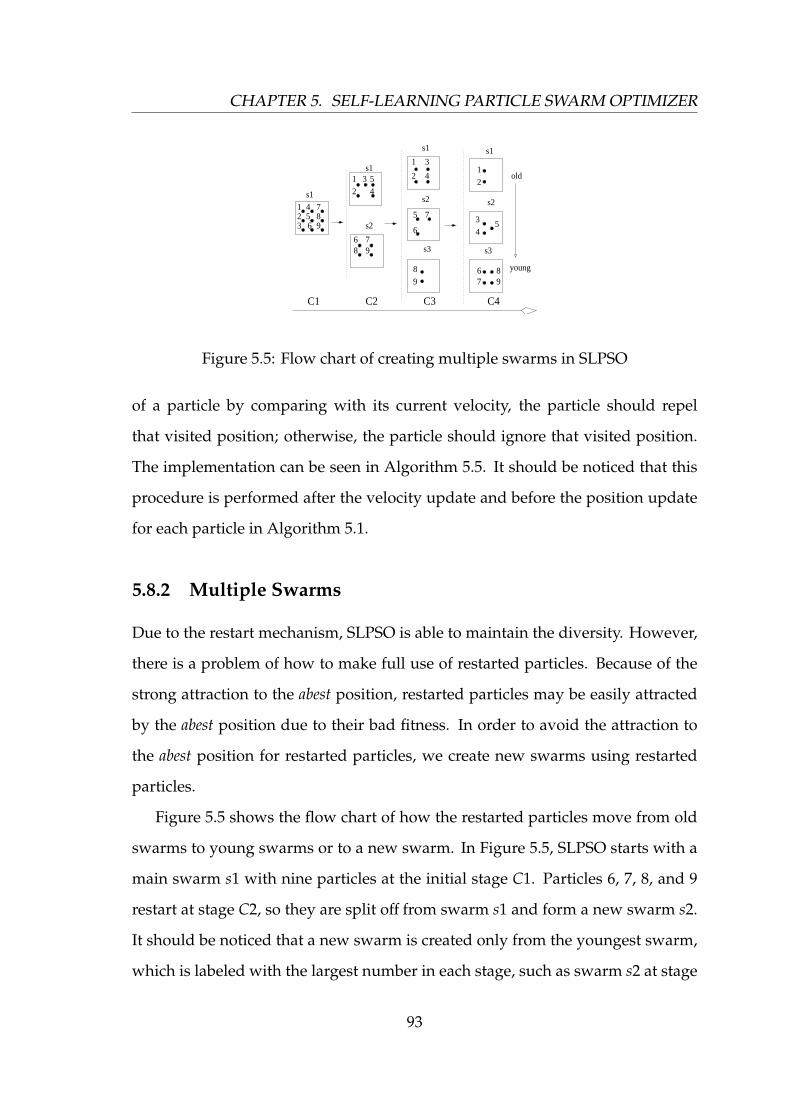
CHAPTER 5. SELF-LEARNING PARTICLE SWARM OPTIMIZER
3
456 9
2
3 5
78 9
1 3
4
7
9
C3
8
C1 C2 C4
712 8
1 2
5
6
1
3
45
2
67
young
s1
s1
s2
s1
s2
s3
s1
s2
s3
old
6
4
98
Figure 5.5: Flow chart of creating multiple swarms in SLPSO
of a particle by comparing with its current velocity, the particle should repel
that visited position; otherwise, the particle should ignore that visited position.
The implementation can be seen in Algorithm 5.5. It should be noticed that this
procedure is performed after the velocity update and before the position update
for each particle in Algorithm 5.1.
5.8.2 Multiple Swarms
Due to the restart mechanism, SLPSO is able to maintain the diversity. However,
there is a problem of how to make full use of restarted particles. Because of the
strong attraction to the abest position, restarted particles may be easily attracted
by the abest position due to their bad fitness. In order to avoid the attraction to
the abest position for restarted particles, we create new swarms using restarted
particles.
Figure 5.5 shows the flow chart of how the restarted particles move from old
swarms to young swarms or to a new swarm. In Figure 5.5, SLPSO starts with a
main swarm s1 with nine particles at the initial stage C1. Particles 6, 7, 8, and 9
restart at stage C2, so they are split off from swarm s1 and form a new swarm s2.
It should be noticed that a new swarm is created only from the youngest swarm,
which is labeled with the largest number in each stage, such as swarm s2 at stage
93

CHAPTER 5. SELF-LEARNING PARTICLE SWARM OPTIMIZER
C2, swarm s3 at stage C3, etc. And a restarted particle always moves from its old
swarm to the next young swarm or a new swarm.
Together with the above components, the implementation of the SLPSO algo-
rithm is summarized in Algorithm 5.6.
5.8.3 Vmax and Out of Search Range Handling in SLPSO
In SLPSO, we use the Vmax parameter to constrain the maximum velocity for each
particle, and the value of Vmax is set to half of the search domain for a general
problem. There are many methods of handling a particle that moves out of the
search range in the literature, e.g., using boundary values, re-initialization, and not
evaluating the particle. In SLPSO, we use a different method to constrain a particle
within the search bounds: for each dimension, before updating its position, we
first remember its position value (xd(t−1)) of the previous iteration, then calculate
a temporal value (xt) by Algorithm 5.1, and finally, update its current position
(xd(t)) as follows:
xd(t) =
R(Xd
min, xd(t − 1)) if xt < Xd
min
R(xd(t − 1),Xdmax) else if xt > Xd
max
xt, else
(5.14)
where R(a, b) returns a uniformly distributed number within (a, b) and [Xdmin,X
dmax]
is the search range of the d-th dimension of the given problem.
5.8.4 Convergence and Diversity in SLPSO
The population convergence speed is one of key performance metrics for EAs and
how to make the population quickly converge is an important issue. Another well-
known open issue in EAs is how to maintain the population diversity. A common
hypothesis is that high diversity is important to avoid premature convergence
94

CHAPTER 5. SELF-LEARNING PARTICLE SWARM OPTIMIZER
Algorithm 5.6 The SLPSO Algorithm1: Generate initial swarm and set up parameters for each particle;2: Set f es :=0, iteration counter for initial swarm t:=0;3: while f es < T Fes do4: for each swarm S[q] do5: for each particle k in swarm S[q] do6: Select one learning operator i using the roulette wheel selection rule;7: Update( i, k, f es);8: Gk
i++; G′ki ++;9: if f (xk(t)) < f (xk(t − 1) then
10: gki++, and set mk := 0;
11: pki+:= f (xk(t − 1)) − f (xk(t));
12: Perform UpdateAbest(k, f es) for the abest position;13: else14: mk := mk + 1;15: end if16: if f (xk(t)) < f (xpbestk) then17: g′ki ++; p′ki +:= f (xpbestk) − f (xk); xpbestk := xk;18: if f (xk) < f (xabest) then19: xabest := xk;20: end if21: end if22: if mk ≥ Uk
f then23: Update the common and monitoring selection ratios according to Eq. (5.8);24: for Each operator j do25: pk
j :=0;gkj :=0; Gk
j :=0; p′kj :=0;g′kj :=0; G′kj :=0;26: end for27: end if28: if 0 <Var(s′k) <= 0.05 then29: Re-initialize particle k; S[q + 1]+:=xk;30: end if31: end for32: UpdatePar();33: t++;34: end for35: end while
where T Fes is the total fitness evaluations for a run and Var(s′k) is the variance of the four monitoring selection ratios
for particle k.
and to escape from local optima. In this section, we will discuss how SLPSO
achieves population convergence and maintains population diversity.
In SLPSO, the convergence operator plays an important role for the population
convergence. This operator will guide all particles to converge to the abest position.
95

CHAPTER 5. SELF-LEARNING PARTICLE SWARM OPTIMIZER
Since the abest position shares its information with all particles by the convergence
operator and it is the best position found by all particles so far, all particles will
eventually converge to the abest position in SLPSO.
From the working mechanism of SLPSO analyzed in the above sections, we
can see that SLPSO has two ways to maintain the population diversity: one
is non-deterministic and the other is deterministic. The non-deterministic way
refers to the jumping-out operator. The jumping-out operator is used to help
particles escape from local optima. Normally, it may help particles explore the
search space in the beginning stage because it has an equal opportunity as the
other three learning operators to be chosen. Then, if the fitness landscape is not
suitable for the jumping-out operator to solve, its selection ratio will drastically
drop to a very low level, which is rare to be selected. However, when particles are
about to converge, the jumping-out operator will be revived due to the punishing
mechanism and might help particles escape from local optima. If it works, the
velocity of a particle can be regained to a certain level of the average velocity of all
particles, which can be seen in Eq. (5.2). This way is non-deterministic, because it
is not guaranteed to happen as the jumping-out operator might not work due to
the improper jumping step.
The second way to maintain the population diversity is through the restart
mechanism. As analyzed above, if none of the four learning operators can help a
particle jump out of the local optimum where it converges, restart will be the last
option to help it escape from that local optimum. After the restart, it will become
an totally active particle again. This way is deterministic because it is guaranteed
to happen for any particle. We take an extreme case where all particles converge
to the global optimum as an example. As we know, none of the four learning
operators works in this case and their selection ratios will absolutely go back to
the initial state. Therefore, the restart mechanism still works.
96

CHAPTER 5. SELF-LEARNING PARTICLE SWARM OPTIMIZER
5.8.5 Complexity of SLPSO
Compared with the basic PSO algorithm, SLPSO needs to perform extra computa-
tion on updating the selection ratios, the abest position, and the three parameters.
For the update of selection ratios and the parameters, we do not need to re-
evaluate particles, and the time complexity is O(N) (N is the population size) for
each iteration. For the abest position update, although we need to re-evaluate
particles, the re-evaluation happens only when particles get improvement, not
every iteration. In addition, for each dimension of the abest position, the update
is performed with a certain probability. According to the above component com-
plexity analysis, we can see that the time complexity of SLPSO is not very high in
comparison with the basic PSO algorithm.
5.9 Summary
In this chapter, we have introduced a novel SLPSO algorithm for global optimiza-
tion problems. In SLPSO, each particle has a set of learning strategies, which are
created by learning from four objectives: its own historical best position, a random
neighbor, the global best position so far, and a random position nearby, respec-
tively. The four learning objectives have different properties, which guide the
particle to converge to the current global best position, exploit a local optimum,
explore new promising areas, and jump out of a local optimum, respectively. In
order to enable particles to automatically choose the appropriate learning objec-
tive at the appropriate moment during the search process, an adaptive selection
mechanism is implemented by an adaptive framework at the individual level.
For each particle, one of the four learning operators is selected according to their
selection ratios. The selection ratio of each operator for each particle is equally
initialized to 1/4 and is updated according to its relative performance.
97

CHAPTER 5. SELF-LEARNING PARTICLE SWARM OPTIMIZER
To increase diversity, we introduce another mechanism to check particles’ evo-
lutionary status by monitoring the performance of the four monitoring operators.
This mechanism enables SLPSO to automatically regain diversity by restarting
those particles that have converged to local optima. Also, there are some other
heuristic rules applied in SLPSO, e.g., extracting useful information from im-
proved particles for the abest position, using an external memory to encourage
each particle to explore new promising sub-regions, and introducing multiple-
swarm methods to avoid the attraction to the exploited abest positions.
In order to make SLPSO effectively work on a general problem, several tech-
niques are introduced. First, a bias selection is given to those badly performing
particles to improve the whole swarm’s performance. Second, to reduce the
risk of punishing the current best operator for a particle because of the temporal
bad performance of that operator in a short period, the selection ratios of the
four learning operators are updated only if a particle is not improved for U f
successive iterations. Third, a learning probability Pl is introduced to solve the
time-consuming problem and to reduce the probability of learning potential bad
information when the abest position learns from an improved particle. Fourth, for
a fair competition among the four learning operators, the scheme of controlling
the number of particles that learn from the abest position is introduced. Finally, the
parameter tuning methods for the three parameters (U f , Pl, and M) are developed
to set up SLPSO for solving a general problem.
98

Chapter 6
Clustering Particle Swarm Optimizer
In the real world, many optimization problems are dynamic. This requires an op-
timization algorithm not only to find the global optimal solution under a specific
environment but also to track the trajectory of the changing optima with time over
dynamic environments. To address this requirement, this chapter investigates a
clustering particle swarm optimizer (CPSO) for DOPs. This algorithm employs
a hierarchical clustering method to locate and track multiple peaks. A fast lo-
cal search method is also introduced to search optimal solutions in a promising
sub-region found by the clustering method.
6.1 Difficulties for PSO in Dynamic Environments
Similar to other EAs in many aspects, PSO has been shown to perform well for
many static problems [85]. However, it is difficult for the basic PSO algorithm to
optimize DOPs. The difficulty lies in two aspects: one is the outdated memory
due to the changing environments and the other is the diversity loss due to the
convergence. Of these two aspects, the diversity loss is by far more serious [10].
It has been demonstrated that the time taken for a partially converged swarm to
re-diversify, find a shifted peak, and then re-converge is quite deleterious to the
99

CHAPTER 6. CLUSTERING PARTICLE SWARM OPTIMIZER
performance of PSO [8].
In the basic PSO algorithm, the diversity loss is mainly due to the strong at-
traction of the global best particle, which results in that all the particles quickly
converge to local or global optimum where the global best particle locates. This
feature is beneficial for many stationary optimization problems. However, for
DOPs, this feature is not good for PSO to track the changing optima. For DOPs, it
is important to guide particles to search in different promising regions to obtain
promising local optima as many as possible because these promising local optima
may become the global best in the next new environment. Hence, local best parti-
cles are needed to guide the search in local regions in the search space. However,
the question becomes how to determine which particles should be suitable as
the neighborhood best and how to assign particles in different neighborhoods to
move toward different sub-regions.
Several PSO algorithms have been recently proposed to address DOPs [10, 40,
41, 84, 117], of which using multi-swarms seems a good technique. The multi-
swarm method can be used to enhance the diversity of the swarm, with the aim
of maintaining multiple swarms on different peaks. The traditional method of
using the multi-swarm method to find optima for multi-modal functions divides
the whole search space into local sub-spaces, each of which may cover one or a
small number of local optima, and then separately search within these sub-spaces.
Here, there are several key, usually difficult, issues aforementioned in Chapter 1,
e.g., how to guide particles to move toward different promising sub-regions, how
to define the area of each sub-region, how to determine the number of sub-swarms
needed, and how to generate sub-swarms. These issues will be further discussed
in the following section.
100
CHAPTER 6. CLUSTERING PARTICLE SWARM OPTIMIZER
6.2 General Considerations for Multi-swarms
In order to address the convergence problem of PSO for DOPs, the multi-swarm
method can be used to maintain multiple swarms on different peaks, which are
referred to as the optima in this thesis. For example, for the MPB problem [13],
the highest peak in the fitness landscape is the global optimum and the other
peaks with a lower height are local optima. Hence, for the multi-swarm method
to work, the whole search space can be divided into several sub-regions. Each
sub-region may contain one or more than one peak. Each sub-swarm covers one
sub-region and exploits it. As mentioned above, when applying the multi-swarm
method to achieve this purpose, there are several key issues to be considered.
The first issue concerns how to guide particles to move toward different
promising sub-regions. This issue is important since if particles can not move
to different sub-regions, PSO can not locate and track multiple optima. This re-
quires that an algorithm should have a good global search capability to explore
promising sub-regions. In [17], the cognitive only PSO model, which was tested
by Kennedy [52], was used to train particles. Since there is no information sharing
among particles in the cognitive only model, each particle just searches around
its personal best position. This may cause the stagnation problem if there are de-
ceptive sub-regions in the search space. Hence, in order to guide particles toward
different promising sub-regions, particles should cooperate with the other nearby
particles.
The second issue concerns how to define the area for each sub-region in the
search space. The area of a sub-region determines how many peaks it may
contain. If the area of a sub-region is too small, there is a potential problem that
small isolated sub-swarms may search on a same local optimum. In this case,
the number of individuals of each sub-swarm may be not enough to make any
progress. However, if a sub-region is too large, there may be more than one peaks
101

CHAPTER 6. CLUSTERING PARTICLE SWARM OPTIMIZER
within the sub-region covered by a sub-swarm. The best situation is that each
sub-region just contains one peak. However, to achieve this goal is very hard
due to the complexity of the search space, especially for real world problems.
Traditionally, the search area of each sub-region is predefined by users according
to preliminary experiments [83] or a formulated estimation [10], and the size of
the search area is the same for all sub-regions. Obviously, it is not true that all the
peaks have exactly the same shape or width in the whole search space. It is very
hard to know the shape of a sub-region. Hence, how to define the search area of a
sub-region is a very hard problem. Ideally, particles within the neighborhood of
a peak should be able to calculate the sub-area by themselves.
How many sub-swarms are needed is the third issue to consider. From the
experimental results in [10], the optimal number of sub-swarms is equal to the total
number of peaks in the whole search space. The more peaks in the search space,
the more sub-swarms we probably need. If too many sub-swarms distribute in
the fitness landscape, the limited computation resources may be wasted. On the
contrary, if there are too small number of sub-swarms, the PSO algorithm can not
efficiently track different local optima. Again, the problem is that the number of
peaks in the search space is usually unknown in advance, especially for real world
problems. Although the number of peaks is given for some benchmark problems,
we should assume that it is unknown to us.
Finally, how to generate sub-swarms is also an open issue. Generally speaking,
sub-swarms are simply obtained by separating the main swarm according to some
mechanism. In [48], a k-means clustering method was used to generate clusters.
The limitation of the k-means method is that the number of clusters must be
predefined. In the speciation based PSO [83], a new species is produced around
a species seed. That is, all the particles within a radius rs distance to a species
seed are classified into a species corresponding to that species seed. Hence, a
102

CHAPTER 6. CLUSTERING PARTICLE SWARM OPTIMIZER
new species is created by a given radius rs around its seed. The number of
sub-swarms is simply predetermined in mCPSO [10], although exclusion and
anti-convergence strategies were used. Exclusion prevents sub-swarms from
covering a single peak by an exclusion radius rexcl, and anti-convergence allows
new peaks to be detected, which was implemented by defining a convergence
radius rconv. However, the serious disadvantage of SPSO and mCPSO is that those
radius parameters must be given. In order to generate sub-swarms as accurate as
possible, that is, only all particles on a same peak form a sub-swarm, the analysis
of population distribution should be done before creating sub-swarms by some
statistical methods.
If particles close to a peak can detect the peak by themselves, then they can
classify themselves into a same cluster, and the search area can also be auto-
matically defined when the new cluster is formed. This thinking motivated the
proposal of CPSO in [69, 134]. In the following section, CPSO in its simplified
version is described in detail to show how it overcomes the above problems when
using the multi-swarm method.
6.3 Framework of the Clustering PSO
To address the above considerations for multi-swarm methods, a clustering
method is introduced in CPSO. The clustering method can enable CPSO to as-
sign particles to different promising sub-regions, adaptively adjust the number
of sub-swarms needed, and automatically calculate the search region for each
sub-swarm.
CPSO starts from an initial swarm, named the cradle swarm. Then, sub-
swarms are created by a hierarchical clustering method. When sub-swarms are
created, local search is launched on them in order to exploit potential peaks cov-
ered by these sub-swarms respectively. Finally, overlapping, convergence, and
103

CHAPTER 6. CLUSTERING PARTICLE SWARM OPTIMIZER
Algorithm 6.1 The CPSO Algorithm1: Create an empty convergence list clst to record the best particles of converged
sub-swarms;2: Create an empty list slst to record sub-swarms;3: Set the fitness evaluation counter evals := 0;4: Generate an initial cradle swarm C randomly;5: Clustering(C, slst);6: while the stop criterion is not satisfied do7: for each sub-swarm slst[i] do8: LocalSearch(slst[i], evals);9: end for
10: CheckSubswarms(C, slst, clst);11: if |C| > 0 then12: LocalSearch(C, evals);13: end if14: if DetectChange(C, slst, clst, evals) then15: Clustering(C, slst);16: end if17: end while
overcrowding checks are performed on the sub-swarms before the next iteration
starts. If an environmental change is detected, a new cradle swarm will be ran-
domly re-generated with the reservation of the positions located by all survived
sub-swarms in the previous environment.
The framework of CPSO for DOPs is given in Algorithm 6.1. In the following
sections, the major components of CPSO, including the clustering method, local
search operator, sub-swarm checks, and detecting environmental changes, are
described in detail, respectively.
6.4 Single Linkage Hierarchical Clustering
Some researchers have used the k-means clustering method to generate sub-
swarms, the problem of the k-means method is that we do not know the optimum
value of k for the current population. In addition, the optimum value of k is
problem dependant. Setting k to a too large or a too small value will cause the
104

CHAPTER 6. CLUSTERING PARTICLE SWARM OPTIMIZER
Algorithm 6.2 Clustering(C, slst)1: Create a temporary cluster list G of size |C|;2: for each particle i in C do3: G[i] :=C[i]; {i.e., each particle forms one cluster in G}4: end for5: Calculate the distance between all clusters (i.e., particles) in G and construct
a distance matrix M of size |G| × |G|;6: while TRUE do7: if FindNearestPair(G, r, s) = FALSE then8: Break;9: end if
10: r := r + s; {i.e., merge clusters r and s into r}11: Delete the cluster s from G;12: Re-calculate all distances in M which have been affected by the merge of r
and s;13: if each cluster in G has more than one particle then14: Break;15: end if16: end while17: slst := G;18: Empty C;
problem of an improper number of sub-swarms, as discussed above. Traditionally,
sub-swarms are created by directly using a number of swarms or simply splitting
off from a main swarm. There is little or no analysis of distribution of individuals
in the search space. Different from traditional clustering methods for multi-swarm
based PSO algorithms, CPSO uses a single linkage hierarchical clustering method
[45], as shown in Algorithm 6.2, to create sub-swarms.
In the clustering method, the distance d(i, j) between two particles i and j in
the D-dimensional space is defined as the Euclidean distance between them as
follows:
d(i, j) =
√√D∑
d=1
(xdi − xd
j )2 (6.1)
The distance of two clusters r and s in G, which is an element in distance matrix
M in Algorithm 6.2 and is denoted as M(r, s), is defined as the distance of the two
105

CHAPTER 6. CLUSTERING PARTICLE SWARM OPTIMIZER
Algorithm 6.3 FindNearestPair(G, r, s)1: f ound := FALSE;
2: min dist :=√∑D
i=1 (Ui − Li)2, where Ui and Li are the upper and lower boundsof the i-th dimension of the search space;
3: for i := 0 to |G| do4: for j := i + 1 to |G| do5: if (|G[i]| + |G[ j]| > max subsize) then6: continue;7: end if8: if (min dist >M(G[i],G[ j])) then9: min dist :=M(G[i],G[ j]);
10: r := G[i];11: s := G[ j];12: f ound := TRUE;13: end if14: end for15: end for16: Return f ound;
closest particles i and j that belong to clusters r and s respectively. M(r, s) can be
formulated as:
M(r, s) = mini∈r, j∈s
d(i, j) (6.2)
Given a cradle swarm C, the clustering method works as follows. It first
creates a list G of clusters with each cluster only containing one particle in C.
Then, in each iteration, it uses Algorithm 6.3 to find a pair of clusters r and s
such that they are the closest among those pairs of clusters, of which the total
number of particles in the two clusters is not greater than max subsize (max subsize
is a prefixed maximum sub-swarm size), and, if successful, combines r and s into
one cluster. This iteration continues until all clusters in G contain more than one
particles. The value of max subsize directly determines how many clusters can be
obtained by the hierarchical clustering method. Definitely, it also determines the
number of sub-swarms.
From the above description, it can be seen that using the above clustering
106

CHAPTER 6. CLUSTERING PARTICLE SWARM OPTIMIZER
method, sub-swarms will be automatically created depending on the distribution
of initial particles in the fitness landscape. The number of sub-swarms and the
size of each sub-swarm are also automatically determined by the fitness landscape
and the unique parameter max subsize.
In this thesis, we have removed the training process used in the original CPSO
[70]. In [70], the aim of training the initial swarm is to guide particles to move
toward different promising sub-regions. After the training process, the clustering
operation will be conducted to generate sub-swarms. From the experimental
results, we found that training for the initial swarm is not necessary. There are
no overlapping search areas among the sub-swarms that are produced from the
initial swarm using the clustering method. Exploitation will then be carried out
immediately in the own local search area of each sub-swarm and the sub-swarms
will gradually move toward the local optima that are close to them, respectively.
Finally, all sub-swarms will distribute in different sub-regions where local optima
are located in the fitness landscape. So, the same objective as the training process
used in the original CPSO [70] can be achieved without training in the simplified
version. The test results regarding CPSO with and without the training process
will be shown later in the experimental study section in Section 8.2.3 in chapter
8. The advantage of removing the training phase in the original CPSO lies in that
more computational resources can be distributed to sub-swarms to perform local
search. The refining clustering operation in the original CPSO is also removed in
the simplified version because the number of sub-swarms can be controlled by
the value of max subsize. Setting a proper value for max subsize can help CPSO
allow one sub-swarm to cover a single peak. So, the refining clustering phase
is also redundant. For example, if we set max subsize to an extreme value (e.g.,
max subsize = 1), then each sub-swarm contains only one particle and can just
cover a single peak.
107

CHAPTER 6. CLUSTERING PARTICLE SWARM OPTIMIZER
Algorithm 6.4 LocalSearch(S, evals)1: for each particle i ∈ S do2: Update particle i according to Eqs. (2.1) and (2.2);3: evals:=++evals%U;4: if particle i is better than pbesti then5: Update pbesti;6: LearnGBest(particle i, gbest, evals);7: if particle i is better than gbest then8: Update gbest;9: end if
10: end if11: end for
It should be noted that it is very difficult for algorithms to track all peaks in
the fitness landscape, especially when we use a limited population resources to
solve a problem with a large number of peaks in the search space. However, we
can just track the peaks that have relatively higher heights compared with the
other peaks in the fitness landscape since these peaks have a higher probability of
becoming the highest peak in the next environment. In CPSO, if one sub-swarm
covers more than one peaks in a local sub-region, particles would focus on the
search on the relatively higher peaks in that local sub-region.
6.5 Local Search Strategy
When a sub-swarm is created using the above clustering method, it will undergo
the local search process in order to exploit the sub-region covered by the sub-
swarm. The framework of the local search process is described in Algorithm 6.4.
In the local search process, in order for a sub-swarm to locate a local peak quickly,
the PSO with the gbest model is used. That is, each particle in a sub-swarm also
learns from the global best position gbest found by the sub-swarm.
In order to speed up the convergence process of sub-swarms, a linear decreas-
ing scheme is also used in CPSO to adjust the inertia weight ω in Eq. (2.1) as
108

CHAPTER 6. CLUSTERING PARTICLE SWARM OPTIMIZER
Algorithm 6.5 LearnGBest(particle i, gbest, evals)1: for each dimension d of gbest do2: xt gbest := xgbest {xt gbest is a temporary particle};3: xt gbest[d] := xi[d];4: if xt gbest is better than xgbest then5: xgbest[d] := xt gbest[d];6: end if7: evals:=++evals%U;8: end for
follows:
ω = ωmax −(ωmax − ωmin) × c itr
r itr(6.3)
whereωmax andωmin are respectively the maximum and minimum value ofω, c itr
is the iteration counter for a sub-swarm, which starts from 0 when a sub-swarm is
newly created, and r itr is the remaining iterations before the next change when
a sub-swarm is created, i.e., r itr = (U − evals)/pop size, where pop size is the total
number of particles in all sub-swarms and the cradle swarm.
In order to extract useful information for the gbest particle in each sub-swarm,
the same idea as used to update the abest position in SLPSO with the learning
probability of 1 is also used in CPSO, which is shown in Algorithm 6.5.
6.6 Check the Status of Sub-swarms
After the local search operation for all sub-swarms, they are checked regarding
overlapping, convergence, and overcrowding. The checking of sub-swarms is as
shown in Algorithm 6.6.
Traditionally, the overlapping check between two sub-swarms is carried out
using their search radius. The search radius of a sub-swarm s can be calculated
as follows.
radius(s) =1|s|∑i∈s
d(i, scenter), (6.4)
109

CHAPTER 6. CLUSTERING PARTICLE SWARM OPTIMIZER
Algorithm 6.6 CheckSubswarms(C, slst, clst)1: for each pair of sub-swarms (r, s) in slst do2: if roverlap(r, s) > Roverlap then3: Merge r and s into r;4: Remove s from slst;5: end if6: end for7: for each sub-swarms r ∈ slst do8: if |r| > max subsize then9: Remove worst (|r| −max subsize) particles from r;
10: end if11: end for12: for each sub-swarms s ∈ slst do13: if radius(s) < Rconv then14: Add gbest into clst;15: Remove s from slst;16: end if17: end for18: if |C| = 0 && |slst| = 0 then19: Add max subsize random particles into C;20: end if
where scenter is the center position of sub-swarm s and |s| is the size of s. If any
particle in a sub-swarm is within the search radius of another sub-swarm, then the
overlapping search is assumed to occur. If the distance of the best particles of two
sub-swarms is less than the sum of their search radius, then they are combined
or one of them is removed. The above checking mechanism assumes that each
sub-swarm just covers one peak. However, it is not true for real PSO algorithms.
If a sub-swarm in a sub-region covers more than one peak, other sub-swarms that
are within its search area should not be removed or combined together with this
sub-swarm.
In order to reduce the risk of losing peaks that are being tracked, we adopt
the following overlapping check scheme in CPSO. If two sub-swarms r and s
are within each other’s search area, an overlapping ratio between them, denoted
roverlap(r, s), is calculated as follows. We first calculate the percentage of particles in
110

CHAPTER 6. CLUSTERING PARTICLE SWARM OPTIMIZER
r which are within the search area of s and the percentage of particles in s which
are within the search area of r, and then set roverlap(r, s) to the smaller one of the two
percentages. The two sub-swarms r and s are combined only when roverlap(r, s) is
greater than a threshold value Roperlap, which is set to 0.7.
In order to avoid too many particles searching on a single peak and hence save
computing resources, an overcrowding check is performed on each sub-swarm
in CPSO after the above overlapping check. If the number of particles in a sub-
swarm is greater than max subsize, then the particles with the worst personal best
positions are removed one by one until the size of the sub-swarm is equal to
max subsize.
For DOPs, the best solutions found in the current environment may be useful
for tracking the movements of peaks in the next environment. Hence, in CPSO,
after the crowding check, the convergence check is carried out to see whether a
sub-swarm has converged. A sub-swarm convergence list clst is used to record the
best positions found by those converged sub-swarms in the current environment.
If the radius of a sub-swarm is less than a small threshold value Rconv, which is set
to 0.0001, the sub-swarm is regarded to be converged on a peak. If a sub-swarm is
converged, its gbest is added into clst in order to be used in the next environment.
Correspondingly, the converged sub-swarm is removed from the sub-swarm list:
slst.
The removal of converged sub-swarm and combining two overlapping sub-
swarms may result in the consequence of no particle surviving. If this happens, the
algorithm will run forever. Therefore, if all sub-swarms are converged, max subsize
random particles will be generated into the current cradle swarm C to deal with
the special situation.
111

CHAPTER 6. CLUSTERING PARTICLE SWARM OPTIMIZER
6.7 Detecting Environmental Changes
Usually, for an algorithm to address DOPs efficiently, it is important to detect
the environmental changes [94]. To detect the environmental changes, we may
use the deterioration of the population performance or the time-averaged best
performance as an indicator [12]. The fitness landscape change will affect all
particles based on our experimental test on the MPB problem. Based on this fact,
we can figure out several simple efficient methods to detect the environmental
changes. Before updating pbest of each particle, we may re-evaluate its pbest
position (e.g., the method used in [84]). If the fitness changes, it means that a
change of the fitness landscape occurs. Another simple approach is to set several
monitoring particles in the search space. The monitoring particles will be re-
evaluated every iteration. If the environment changes, it will be detected by these
monitoring particles using the above detecting method.
In CPSO, we use the global best particle over all sub-swarms as the moni-
toring particle to detect the environmental changes. Before updating the global
best particle, we re-evaluate its fitness at each iteration. If its fitness changes, it
indicates that an environmental change occurs. Once an environmental change
is detected, CPSO takes the following actions, as shown in Algorithm 6.7; other-
wise, if it fails to detect the change, the previous population will be used in the
new environment. In order to adapt to the new environment quickly, we take the
following actions. First, the best position gbest of each sub-swarm in slst before
the change is saved into clst. Then, all particles are re-initialized to create a new
cradle swarm and the particles stored in clst are added to the new cradle swarm
by replacing the worst particles in it. Finally, slst and clst are re-set to be empty.
Again, the clustering method will be performed to generate the new sub-swarm
list.
112

CHAPTER 6. CLUSTERING PARTICLE SWARM OPTIMIZER
Algorithm 6.7 DetectChange(C, slst, clst, evals)1: Re-evaluate the global best particle over all sub-swarms;2: evals :=++evals%U;3: if The fitness of the re-evaluated position changes then4: Save the gbest of each sub-swarm in slst into clst;5: Remove all sub-swarms in slst;6: Generate a new cradle swarm C;7: Add the particles in clst into C;8: Empty clst;9: Return TRUE;
10: else11: Return FALSE;12: end if
6.8 Complexity Analysis
The major components of CPSO are the clustering operation, local search, and
status checking of each sub-swarm. The clustering operation is performed only
once at the very beginning when an environmental change is detected. From
Algorithm 6.2, it can be seen that the time complexity of the clustering operation
is O(N3), where N is the population size of the cradle swarm. We first compute
all distances among each pair of particles in O(N2). For each iteration of merging
two clusters r and s from the cluster list G, we find the nearest pair of clusters
of G in O(|G|2) (if we use dynamic programming method, it would be reduced
to O(|G|log(|G|))), then update the distance matrix M in O(|G|). The number of
clusters in G will decrease by 1 every iteration until the stop criterion is met.
Finally, we perform the clustering operation in O(N3).
In the local search operation (Algorithm 6.4) for each sub-swarm, except per-
forming the gbest learning on improved particles, there is no big difference from
the basic PSO algorithm. In addition, the time complexity will reduce as perform-
ing overlapping and overcrowding check because of decreasing number of total
particles.
The time complexity of the sub-swarm status check depends on how many
113

CHAPTER 6. CLUSTERING PARTICLE SWARM OPTIMIZER
sub-swarms are produced by the clustering operation. However, it also will
decrease as performing overlapping and convergence check for sub-swarms. In
total, according to the above component complexity analysis, the extra computing
time needed for CPSO is not so high in comparison with the basic PSO algorithm.
6.9 Comparison between CPSO and PSO with the
lbest Model
In the PSO with the lbest model (PSOlbest), if we define the neighborhood of a parti-
cle as its nearest max subsize particles, and assign the best one of its neighborhood
as its social component in Eqs. (2.1), it seems that we will get a similar search
behavior as CPSO. This is because the clustering method in CPSO will assign the
particles that are close to each other into a sub-swarm, which is the same as the
neighborhood defined in PSOlbest. However, CPSO has several major advantages
in comparison with PSOlbest.
First, CPSO can track multiple optima in dynamic environments. In CPSO, if
more than one sub-swarms cover a same peak, they will finally be combined with
each other into one sub-swarm by the overlapping check function. Hence, the
positions found by the converged sub-swarms in clst are distributed on different
peaks. Once an environmental change occurs, the elements in clst will be added
into the new cradle swarm. When a peak moves not too far away from the
previous location, the previous peak position locates on the slope of the new
current peak. As we know, if this case happens, the previous peak location does
help the search of the current peak in the new environment. However, PSOlbest
can not recognize such kind of peak locations even they are found by PSOlbest. It is
impossible to directly check which particles in the whole swarm are from different
peaks since different peaks have quite different heights. Therefore, PSOlbest can
114

CHAPTER 6. CLUSTERING PARTICLE SWARM OPTIMIZER
not track multiple optima in dynamic environments.
Second, CPSO can control overcrowding in a single peak. There are two
aspects regarding the overcrowding over a single peak in CPSO. One is that more
than one sub-swarms cover a single peak, and the other is that too many particles
exist within one sub-swarm on a peak. The first problem can be solved by the
overlapping check as analyzed above. Hence, those sub-swarms that are inferior
to the best sub-swarm on a peak will be automatically removed. The second
problem is solved by the overcrowding check in Algorithm 6.6. However, PSOlbest
can not solve the overcrowding problem since it can not check which particles
locate on which peaks.
Third, CPSO has a higher probability of covering more local optima than
PSOlbest can do. In CPSO, since there is no communication among sub-swarms,
each sub-swarm just searches its local area, and finally will converge to a local
optimum if it survives till the next change takes place. Hence, every peak will
be found if it is covered by a sub-swarm. However, in PSOlbest, the gbest with a
relatively better fitness of one particle’s neighborhood may belong to the neigh-
borhood of different particles. That is, particles from different peaks may share
the same gbest. So, particles from the peaks with lower heights will be attracted
by the gbest from the peak with a higher height. Finally, they will converge on that
peak with a higher height and lose the track of the peaks with relatively lower
heights.
Finally, CPSO can partially adaptively adjust the number of particles and sub-
swarms needed to achieve the best performance based on its work mechanism.
However, the number of particles in PSOlbest is fixed during the whole run.
115

CHAPTER 6. CLUSTERING PARTICLE SWARM OPTIMIZER
6.10 Summary
This chapter introduced a clustering PSO for DOPs to locate and track multiple
peaks using the multiple swarm method. The single linkage hierarchical clus-
tering method used in CPSO, which is the major contribution of the algorithm,
solves several key issues when using the multiple swarm method, e.g., how to
guide particles to move toward different promising sub-regions, how to define
the area of each sub-region, how to determine the number of sub-swarms needed,
and how to generate sub-swarms.
In addition, to improve the effectiveness of CPSO, several techniques are im-
plemented in CPSO to check the status regarding overlapping, convergence, and
overcrowding.
116

Chapter 7
Experimental Study of SLPSO
It is very hard to give an accurate analysis of a real PSO algorithm’s performance
(e.g., convergence and diversity) due to its stochastic movement. One strategy
adopted to analyze a PSO algorithm’s performance is to choose a set of functions
that have different properties and levels of complexity, and compare the best
solutions achieved by the algorithm with the global optima of the selected test
functions. Another method to examine an algorithm’s performance is to compare
the algorithm with some state-of-the-art algorithms.
In this chapter, the experimental study of the SLPSO algorithm is performed
based on the static problems ( f1- f45) introduced in Chapter 3. In order to examine
the ideas used in SLPSO and provide some evidence, the experimental study,
including the analysis of the search behavior, the adaptive learning mechanism,
the parameter sensitivity analysis, the learning strategy for the abest position, and
the process of selection ratios of the four learning operators, are performed. In
addition, some state-of-the-art PSO algorithms are chosen, including CPSO-Hk
[115], FIPS [76], CLSPO [43], and APSO [138] as well as the standard PSO (SPSO)
[14], to further test the performance of SLPSO.
117

CHAPTER 7. EXPERIMENTAL STUDY OF SLPSO
Table 7.1: Configuration of Involved PSO AlgorithmsAlgorithm Year Population Topology Parameter SettingsSPSO[14] 2007 Local ring ω=0.721348, η1=η2=1.19315CPSO-Hk[115] 2004 Cooperative multi- ω: [0.4, 0.9], η1 = η2 = 1.49
swarm approach k=6FIPS[76] 2004 Local URing χ = 0.7298,
∑ci = 4.1
CLPSO[43] 2006 Comprehensive learning ω: [0.4, 0.9], η = 2.0APSO[138] 2009 Global star ω: [0.4, 0.9], η1 + η2: [3.0, 4.0]
with adaptive tuning
7.1 Experimental Setup
Experiments were conducted to compare SLPSO with the five PSO algorithms on
the 45 test problems in 10, 30, and 50 dimensions, respectively. The configuration
of each peer algorithm, which is exactly the same as it appeared in the original
paper, is given in Table 7.1.
Below is a brief description of the peer PSO algorithms taken from the literature
to compare with SLPSO. The first algorithm is the cooperative PSO (CPSO-Hk)
[115], which combines a cooperative PSO model with the original PSO. For this
algorithm, we also use the same value of “split factor” k = 6 as it was used in
the original paper [115]. The second algorithm is the fully informed PSO (FIPS)
[76] with a U-ring topology that achieved the highest success rate. The third
algorithm is the comprehensive learning PSO (CLSPO) [43], which was proposed
for solving multi-modal problems and shows a good performance in comparison
with eight other PSO algorithms. The fourth peer algorithm is the adaptive
PSO (APSO) [138], which adaptively tunes the values of η1, η2, andω based on the
population distribution in the fitness landscape to achieve different purposes, such
as exploration, exploitation, jumping out, and convergence. It was reported that
APSO substantially enhanced the performance of PSO in terms of the convergence
speed, the global optimality, the solution accuracy, and the algorithm reliability.
118

CHAPTER 7. EXPERIMENTAL STUDY OF SLPSO
The fifth peer algorithm is the standard PSO (SPSO) proposed in [14]. We chose
this algorithm to investigate how SLPSO performs compared to the standard
version of PSO. For SLPSO, η1 and η2 were set to 1.496. Vmax was set to half of
the search domain for each test function, which can be seen from Table 3.1 and
Table 3.3, and the default parameter settings suggested in Section 5.7 were used
for all problems if there is no special note.
To fairly compare SLPSO with the other five algorithms, all algorithms were
run independently 30 times on the 45 test problems. The initial population and the
stop criterion are the same for all algorithms for each run. The maximal number of
fitness evaluations (T Fes) was used as the stop criterion for all algorithms on each
test function. The swarm size and T Fes were set to (10, 50000), (20, 100000), and
(30, 300000) for dimensions 10, 30, and 50, respectively. The parameter settings of
the other five algorithms are based on their optimal configurations suggested by
the corresponding papers.
7.2 Working Mechanism of SLPSO
In this section, the experimental study, including the search behavior, the self-
learning mechanism, parameter sensitivity analysis, the learning strategy for the
abest position, and the common selection ratios of the four learning operators, is
performed to examine the performance of SLPSO.
7.2.1 Analyzing the Search Behavior of SLPSO
This section provides evidence to support our assumption of SLPSO’s working
mechanism on the unimodal Sphere function ( f1) and multi-modal Schwefel func-
tion ( f6) in two dimensions. For simplicity, we only used five particles on both test
functions over a single run of 10000 total fitness evaluations and all five particles
119

CHAPTER 7. EXPERIMENTAL STUDY OF SLPSO
-100
-50
0
50
100
-100 -50 0 50 100
Trajectories of Particles’ pbest position
p1p2
p3
p4
p5G
-400
-200
0
200
400
-400 -200 0 200 400
Trajectories of Particles’ pbest position
p1p2
p3
p4
p5
G
-400
-350
-300
-250
-200
-150
-100
-50
0
50
0 2 4 6 8
fitn
ess
(log
)
evals (x1000)
p1p2p3p4p5
0
200
400
600
800
1000
1200
0 2 4 6 8 10
fitn
ess
evals (x1000)
p1p2p3p4p5
-180-160-140-120-100-80-60-40-20
0 20
0 2 4 6 8
velo
city
(log
)
evals (x1000)
Particles’ velocity
p1p2p3p4p5
-90-80-70-60-50-40-30-20-10
0 10
0 2 4 6 8 10
velo
city
(log
)
evals (x1000)
Particles’ velocity
p1p2p3p4p5
Figure 7.1: pbest trajectory, fitness process, and velocity of each particle on theSphere function (left) and Schwefel function (right) in two dimensions
use the four learning operators from the beginning to the end of the evolution. In
other words, different from the original SLPSO algorithm, there is no control of
using the convergence operator for all particles.
Figure 7.1 shows the pbest trajectory, fitness process, and velocity process of the
five particles on the Sphere and Schwefel functions, where the circle points labeled
with “G” of the top two graphs are the locations of the global optima of the two
functions. The five particles start the search at the locations of “Pi”, i = 1, 2, . . . , 5.
The graphs on the left hand are the results on the Sphere function and the graphs
on the right hand are the results on the Schwefel function. Figure 7.2 and Figure 7.3
120
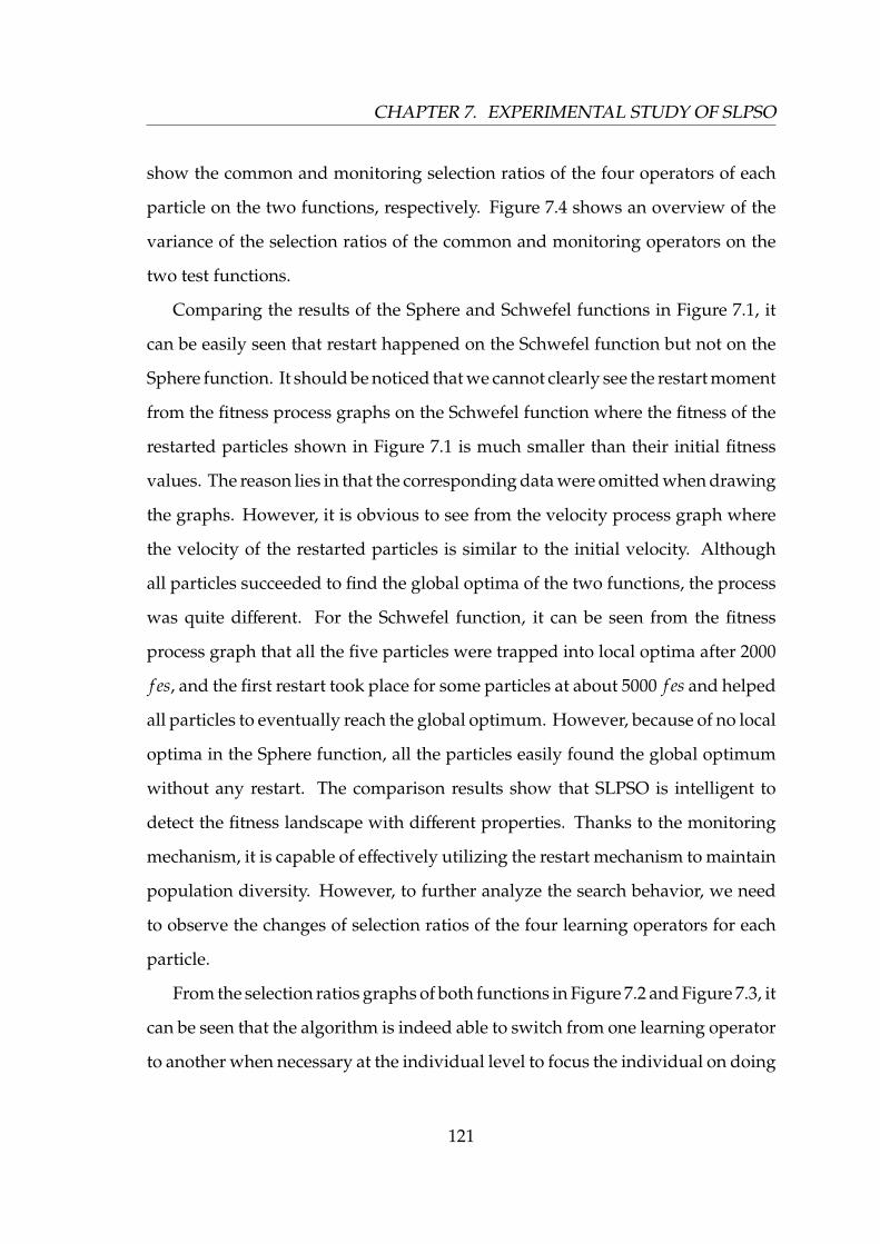
CHAPTER 7. EXPERIMENTAL STUDY OF SLPSO
show the common and monitoring selection ratios of the four operators of each
particle on the two functions, respectively. Figure 7.4 shows an overview of the
variance of the selection ratios of the common and monitoring operators on the
two test functions.
Comparing the results of the Sphere and Schwefel functions in Figure 7.1, it
can be easily seen that restart happened on the Schwefel function but not on the
Sphere function. It should be noticed that we cannot clearly see the restart moment
from the fitness process graphs on the Schwefel function where the fitness of the
restarted particles shown in Figure 7.1 is much smaller than their initial fitness
values. The reason lies in that the corresponding data were omitted when drawing
the graphs. However, it is obvious to see from the velocity process graph where
the velocity of the restarted particles is similar to the initial velocity. Although
all particles succeeded to find the global optima of the two functions, the process
was quite different. For the Schwefel function, it can be seen from the fitness
process graph that all the five particles were trapped into local optima after 2000
f es, and the first restart took place for some particles at about 5000 f es and helped
all particles to eventually reach the global optimum. However, because of no local
optima in the Sphere function, all the particles easily found the global optimum
without any restart. The comparison results show that SLPSO is intelligent to
detect the fitness landscape with different properties. Thanks to the monitoring
mechanism, it is capable of effectively utilizing the restart mechanism to maintain
population diversity. However, to further analyze the search behavior, we need
to observe the changes of selection ratios of the four learning operators for each
particle.
From the selection ratios graphs of both functions in Figure 7.2 and Figure 7.3, it
can be seen that the algorithm is indeed able to switch from one learning operator
to another when necessary at the individual level to focus the individual on doing
121

CHAPTER 7. EXPERIMENTAL STUDY OF SLPSO
0
0.2
0.4
0.6
0.8
1
0 2 4 6 8
Com
mon
sel
ectio
n ra
tios
evals (x1000)-particle 1
exploitation jumping-out exploration convergence
0
0.2
0.4
0.6
0.8
1
0 2 4 6 8
Mon
itori
ng s
elec
tion
ratio
s
evals (x1000)-particle 1
exploitation jumping-out exploration convergence
0
0.2
0.4
0.6
0.8
1
0 2 4 6 8
Com
mon
sel
ectio
n ra
tios
evals (x1000)-particle 2
exploitation jumping-out exploration convergence
0
0.2
0.4
0.6
0.8
1
0 2 4 6 8
Mon
itori
ng s
elec
tion
ratio
s
evals (x1000)-particle 2
exploitation jumping-out exploration convergence
0
0.2
0.4
0.6
0.8
1
0 2 4 6 8
Com
mon
sel
ectio
n ra
tios
evals (x1000)-particle 3
exploitation jumping-out exploration convergence
0
0.2
0.4
0.6
0.8
1
0 2 4 6 8
Mon
itori
ng s
elec
tion
ratio
s
evals (x1000)-particle 3
exploitation jumping-out exploration convergence
0
0.2
0.4
0.6
0.8
1
0 2 4 6 8
Com
mon
sel
ectio
n ra
tios
evals (x1000)-particle 4
exploitation jumping-out exploration convergence
0
0.2
0.4
0.6
0.8
1
0 2 4 6 8
Mon
itori
ng s
elec
tion
ratio
s
evals (x1000)-particle 4
exploitation jumping-out exploration convergence
0
0.2
0.4
0.6
0.8
1
0 2 4 6 8
Com
mon
sel
ectio
n ra
tios
evals (x1000)-particle 5
exploitation jumping-out exploration convergence
0
0.2
0.4
0.6
0.8
1
0 2 4 6 8
Mon
itori
ng s
elec
tion
ratio
s
evals (x1000)-particle 5
exploitation jumping-out exploration convergence
Figure 7.2: Selection ratios of the common and monitoring operators on the Spherefunction ( f1) in two dimensions
122

CHAPTER 7. EXPERIMENTAL STUDY OF SLPSO
0
0.2
0.4
0.6
0.8
1
0 2 4 6 8 10
Com
mon
sel
ectio
n ra
tios
evals (x1000)-particle 1
exploitation jumping-out exploration convergence
0
0.2
0.4
0.6
0.8
1
0 2 4 6 8 10
Mon
itori
ng s
elec
tion
ratio
s
evals (x1000)-particle 1
exploitation jumping-out exploration convergence
0
0.2
0.4
0.6
0.8
1
0 2 4 6 8
Com
mon
sel
ectio
n ra
tios
evals (x1000)-particle 2
exploitation jumping-out exploration convergence
0
0.2
0.4
0.6
0.8
1
0 2 4 6 8
Mon
itori
ng s
elec
tion
ratio
s
evals (x1000)-particle 2
exploitation jumping-out exploration convergence
0
0.2
0.4
0.6
0.8
1
0 2 4 6 8 10
Com
mon
sel
ectio
n ra
tios
evals (x1000)-particle 3
exploitation jumping-out exploration convergence
0
0.2
0.4
0.6
0.8
1
0 2 4 6 8 10
Mon
itori
ng s
elec
tion
ratio
s
evals (x1000)-particle 3
exploitation jumping-out exploration convergence
0
0.2
0.4
0.6
0.8
1
0 2 4 6 8 10
Com
mon
sel
ectio
n ra
tios
evals (x1000)-particle 4
exploitation jumping-out exploration convergence
0
0.2
0.4
0.6
0.8
1
0 2 4 6 8 10
Mon
itori
ng s
elec
tion
ratio
s
evals (x1000)-particle 4
exploitation jumping-out exploration convergence
0
0.2
0.4
0.6
0.8
1
0 2 4 6 8 10
Com
mon
sel
ectio
n ra
tios
evals (x1000)-particle 5
exploitation jumping-out exploration convergence
0
0.2
0.4
0.6
0.8
1
0 2 4 6 8 10
Mon
itori
ng s
elec
tion
ratio
s
evals (x1000)-particle 5
exploitation jumping-out exploration convergence
Figure 7.3: Selection ratios of the common and monitoring operators on theSchwefel function ( f6) in two dimensions
123

CHAPTER 7. EXPERIMENTAL STUDY OF SLPSO
0
0.2
0.4
0.6
0.8
1
0 2 4 6 8 10
varia
nce
of s
elec
tion
ratio
s
evals (x1000)-particle 1
commonmonitor
0
0.2
0.4
0.6
0.8
1
0 2 4 6 8 10
varia
nce
of s
elec
tion
ratio
s
evals (x1000)-particle 1
commonmonitor
0
0.2
0.4
0.6
0.8
1
0 2 4 6 8 10
varia
nce
of s
elec
tion
ratio
s
evals (x1000)-particle 2
commonmonitor
0
0.2
0.4
0.6
0.8
1
0 2 4 6 8 10va
rianc
e of
sel
ectio
n ra
tios
evals (x1000)-particle 2
commonmonitor
0
0.2
0.4
0.6
0.8
1
0 2 4 6 8 10
varia
nce
of s
elec
tion
ratio
s
evals (x1000)-particle 3
commonmonitor
0
0.2
0.4
0.6
0.8
1
0 2 4 6 8 10
varia
nce
of s
elec
tion
ratio
s
evals (x1000)-particle 3
commonmonitor
0
0.2
0.4
0.6
0.8
1
0 2 4 6 8 10
varia
nce
of s
elec
tion
ratio
s
evals (x1000)-particle 4
commonmonitor
0
0.2
0.4
0.6
0.8
1
0 2 4 6 8 10
varia
nce
of s
elec
tion
ratio
s
evals (x1000)-particle 4
commonmonitor
0
0.2
0.4
0.6
0.8
1
0 2 4 6 8 10
varia
nce
of s
elec
tion
ratio
s
evals (x1000)-particle 5
commonmonitor
0
0.2
0.4
0.6
0.8
1
0 2 4 6 8 10
varia
nce
of s
elec
tion
ratio
s
evals (x1000)-particle 5
commonmonitor
Figure 7.4: Process of variance of common and monitoring selection ratios of thefour learning operators on the Sphere function (left) and the Schwefel function(right) in two dimensions
124

CHAPTER 7. EXPERIMENTAL STUDY OF SLPSO
one of the following task: exploration, exploitation, convergence, or jumping out.
In both Sphere and Schwefel problems, each particle was able to choose a new best
learning objective when it could not get benefit from the old, outdated learning
objective.
For particles in different sub-regions in the fitness landscape, the learning
strategies with the largest selection ratios are different. In other words, SLPSO is
capable to adapt to different environments by using different learning strategies.
Take the Sphere function as an example. To reach the position of the global
optimum, particles 1 and 4 used the exploration operator from the beginning to
the end, while particles 2 and 3 switched between the exploration and exploitation
operators several times during the whole evolutionary process. However, for
particle 5, the most frequently used strategy was the convergence operator.
By comparing the common and monitoring selection ratios of the four learning
operators on the Schwefel function, we can clearly see a particle’s convergence
status through the monitoring selection ratios but not through the common se-
lection ratios. Take particle 1 as an example. The convergence status was shown
twice when it converged in the monitoring selection ratios graph where the val-
ues of the four learning operators went back to the initial state. However, we
cannot observe this trend in the corresponding common selection ratio graph.
This validates our assumption that the common selection ratios cannot monitor
a particle’s status. On the contrary, for the graphs of the Sphere function in Fig-
ure 7.4, we cannot see the similar observations as on the Schwefel function as no
re-initialization happened for the five particles and the process of the common
and monitoring selection ratios has similar trend for all the five particles during
the whole evolutionary process.
It should be noticed that the common selection ratios did show the initial state
where they have equal values during the evolutionary process in Figure 7.3 and the
125

CHAPTER 7. EXPERIMENTAL STUDY OF SLPSO
variance of the common selection ratios becomes 0 in Figure 7.4. This is because the
common selection ratios of the four learning operators were reset to initial states
when particles were re-initialized. This can be clearly seen from Figure 7.4. The
results on the Schwefel function in Figure 7.4 obviously show that the variance
of the monitoring selection ratios linearly decreases when particles tend to be
convergence status till the restart happened. However, although particles are in
the convergence status, the variance of common selection ratios is still in a very
large level. For the Sphere function, we cannot observe the similar phenomenon
with the monitoring selection ratios as for the Schwefel function.
By observing the search behavior of SLPSO on unimodal (Sphere) and multi-
modal (Schwefel) problems, we can conclude that the adaptive learning mecha-
nism does enable SLPSO to deal with different situations at the individual level. In
other words, each single particle is able to learn the knowledge of its surrounding
local area and also is able to check its own evolutionary status so that it can make
right decisions for some hard situations, e.g., which learning strategy should be
used, how to check the convergence status, and when to restart if being trapped
into local optimum, to adapt to the changing environments. By considering these
issues, each particle can automatically change its search behavior according to the
surrounding environments and its evolutionary status.
7.2.2 Self-Learning Mechanism Test
In order to further investigate the level of effectiveness that the adaptive learning
mechanism can bring to SLPSO, we carried out experiments on SLPSO with the
adaptive learning mechanism and on Non-SLPSO without the adaptive learning
mechanism over all the test functions in 30 dimensions. For SLPSO, the default
parameter settings were used. In Non-SLPSO, all the four learning operators have
an equal selection ratio of 0.25 during the whole evolutionary process. Table 7.2
126

CHAPTER 7. EXPERIMENTAL STUDY OF SLPSO
Table 7.2: Comparison with random selection for the four learning operatorsregarding the mean value
f f1 f2 f3 f4 f5 f6 f7 f8 f9Random 1.52e-13 7.47e-10 7.08e-07 1.34e-04 0.0168504 3.82e-04 8.99e-08 23.5034 1.39e-07Adaptive 6.32e-50 0 0 4.50e-15 0.00816972 3.82e-04 4.05e-14 7.34554 3.32e-28
f f10 f11 f12 f13 f14 f15 f16 f17 f18Random 30.7624 1.32e-04 2.49e-15 90.7131 90.3314 3.82e-04 0.001151 2.18e-05 4.21e-05Adaptive 0.185749 0.369122 1.57e-32 20.0509 20.4416 3.82e-04 3.29e-14 0 0
f f19 f20 f21 f22 f23 f24 f25 f26 f27Random 4.31e-04 3.94842 0.015133 0.088096 1.03e-12 214.611 6556.43 3.67856 1.22e-04Adaptive 6.47e-04 5.46e-04 0.01918 0.122745 5.87e-46 115.579 4575.08 4.50667 0
f f28 f29 f30 f31 f32 f33 f34 f35 f36Random 6954.29 20.8023 161.818 4.19e-05 2.88e-05 157.64 34.366 20.7782 65.9935Adaptive 4948.79 20.6376 105.687 1.29e-13 1.21e-13 114.67 30.4103 20.5754 8.20752
f f37 f38 f39 f40 f41 f42 f43 f44 f45Random 228.201 14676 0.642808 336.844 420.118 607.911 913.073 433.022 296.972Adaptive 0.0694798 14277.4 1.31e-13 290.464 414.28 986.578 1179.03 399.39 307.761
presents the results on the 45 functions for SLPSO and Non-SLPSO.
From Table 7.2, it can be seen that the results of SLPSO are much better than
that of Non-SLPSO on 36 functions out of the total 45 test problems. The reason
for the problems where the results of SLPSO are worse than those of Non-SLPSO
is because improper parameter values were used. This can be seen from the com-
parison of SLPSO with the default configurations and the optimal configurations
in the following section where the performance of SLPSO is greatly improved
when the optimal configuration are used. The comparison result shows that the
adaptive mechanism works well on most problems. And it also confirms that
different problems need different strategies to solve. To achieve the best perfor-
mance, it is necessary to tune the selection ratios of the four learning operators so
that the best learning strategy can effectively play a role.
7.2.3 Parameter Sensitivity Analysis of SLPSO
To find out how the parameters affect the performance of SLPSO, an experiment
on parameter sensitivity analysis of SLPSO was also conducted on all the 45
problems in 30 dimensions. The key parameters include the update frequency
127

CHAPTER 7. EXPERIMENTAL STUDY OF SLPSO
Table 7.3: Effect of the update frequencyU f f1 f2 f3 f4 f5 f6 f7 f8 f91 9.49e-33 0 0 1.37e-14 0.0198629 19.7401 5.36e-14 4.19863 3.38e-173 1.12e-29 0 0 1.09e-14 0.0179618 7.89627 5.89e-14 6.19834 2.45e-167 1.64e-22 0 0 8.19e-13 0.0261546 31.5839 1.10e-11 10.7329 1.17e-1210 5.01e-19 2.37e-16 1.37e-13 1.33e-09 0.0186557 11.8442 6.13e-11 12.3649 5.08e-11U f f10 f11 f12 f13 f14 f15 f16 f17 f181 0.00855641 0.0118861 1.57e-32 66.6667 169.293 19.7401 5.16e-14 0 03 0.0219023 3.40e-04 5.66e-29 66.6667 178.059 11.8442 6.23e-14 0 5.39e-277 1.07724 3.79e-05 2.47e-21 66.6667 231.113 11.8442 2.24e-12 0 2.60e-2210 3.12558 4.91e-05 6.24e-19 66.6667 226.873 3.82e-04 1.73e-11 0 2.26e-20U f f19 f20 f21 f22 f23 f24 f25 f26 f271 7.20e-04 23.6881 0.0194899 0.129472 1.69e-29 178.468 5527.69 8.40049 4.01e-303 8.57e-04 7.89635 0.0210841 0.123632 2.95e-28 177.628 5628.55 5.37123 1.68e-257 7.11e-04 3.94843 0.0187445 0.104331 6.68e-20 191.285 5770.61 5.01039 2.78e-2110 6.33e-04 7.89636 0.0196384 0.13006 4.36e-18 208.603 6123.21 6.50096 2.96e-19U f f28 f29 f30 f31 f32 f33 f34 f35 f361 6119.39 20.5861 136.602 1.50e-13 1.33e-13 149.809 31.6188 20.5105 11.1313 6502.66 20.6557 135.463 1.42e-13 1.38e-13 127.238 32.8685 20.5092 15.18887 6380.69 20.7836 136.813 1.46e-13 1.31e-13 127.436 32.9158 20.7317 15.796710 6550.11 20.8193 133.155 1.61e-13 1.67e-13 122.834 33.4664 20.8005 16.6575U f f37 f38 f39 f40 f41 f42 f43 f44 f451 0.00314017 20074.9 1.61e-13 270 456.783 1074.81 1313.41 520.227 322.2313 0.00718157 18885.6 1.55e-13 270 443.597 1069.83 1464.8 511.16 344.8077 0.132277 17770.5 2.18e-13 270 451.379 935.929 1524.22 499.565 311.21810 0.745756 18413.8 2.25e-13 250.716 484.477 912.493 1472.35 536.127 333.969
(U f ), the learning probability (Pl), and the number of particles that learn from
the abest position (M, which is replaced with percentages of population size for
convenience here). The default values of the three parameters are set to 10,1.0,
and 1.0, respectively. To separately test the effect of a particular parameter, we
used the default values of the other two parameters. For example, to test the effect
of U f , we choose a set of values for U f and use the default values for Pl =1.0 and
M =1.0, respectively.
Three groups of experiments with U f in the set [1,3,7,10], Pl in the set [0.05,0.1,
0.3,0.7,1.0], and M in the set [0.0,0.1,0.3,0.7,1.0] were carried out separately and
the corresponding results are summarized in Table 7.3, Table 7.4, and Table 7.5,
respectively. Figure 7.5 shows the statistical results of the number of problems
where SLPSO achieves the best result with each particular parameter.
For the parameter U f , as already mentioned in Section 5.3.3 in Chapter 5,
the optimal value of U f for a specific problem depends on the property of that
128

CHAPTER 7. EXPERIMENTAL STUDY OF SLPSO
Table 7.4: Effect of the learning probabilityPl f1 f2 f3 f4 f5 f6 f7 f8 f9
0.05 1.27e-61 0.0994959 0.0333333 1.95e-04 0.0184491 367.159 2.24e-14 6.31095 3.02e-300.1 1.99e-86 1.18e-16 1.78e-16 5.33e-07 0.0148208 228.981 2.03e-14 3.37152 1.73e-500.3 1.43e-62 0 0 1.42e-15 0.0195018 43.4278 2.98e-14 4.86947 4.05e-330.7 1.59e-27 0 0 6.87e-15 0.0140862 3.94833 5.44e-14 10.5145 2.21e-151 5.01e-19 2.37e-16 1.37e-13 1.33e-09 0.0186557 11.8442 6.13e-11 12.3649 5.08e-11Pl f10 f11 f12 f13 f14 f15 f16 f17 f18
0.05 0.0361189 1.16228 4.04e-32 30 56.6667 403.179 1.20e-14 0.709638 8.94e-300.1 0.00513775 0.204989 1.69e-32 26.6667 56.6667 197.359 1.45e-14 0.203381 00.3 0.00145181 0.0144136 1.57e-32 92.6254 123.333 58.4005 2.33e-14 0 00.7 0.176488 8.74e-05 2.27e-27 96.8129 144.652 23.688 5.36e-14 0 5.46e-281 3.12558 4.91e-05 6.24e-19 66.6667 226.873 3.82e-04 1.73e-11 0 2.26e-20Pl f19 f20 f21 f22 f23 f24 f25 f26 f27
0.05 2.08e-04 390.847 0.0101869 0.0852683 8.16e-32 84.3764 3876.63 3.46848 2.92e-280.1 2.04e-04 213.189 0.0104484 0.0435477 1.32e-64 101.493 4239.88 3.05643 2.82e-300.3 2.96e-04 35.5319 0.0125978 0.0615876 1.33e-59 148.328 4626.1 3.48268 00.7 5.85e-04 3.94839 0.0171477 0.0985399 1.66e-26 166.257 5965.69 4.5377 5.90e-271 6.33e-04 7.89636 0.0196384 0.13006 4.36e-18 208.603 6123.21 6.50096 2.96e-19Pl f28 f29 f30 f31 f32 f33 f34 f35 f36
0.05 4168.09 20.7942 91.8854 6.44e-14 1.42611 84.7878 28.0658 20.7632 6.942650.1 4483.06 20.7503 81.085 6.06e-14 0.431149 95.3393 27.8497 20.7512 2.946070.3 5142.13 20.7779 122.312 9.09e-14 9.76e-08 102.124 31.2341 20.7244 3.516370.7 5648.19 20.7756 125.938 1.25e-13 1.12e-13 129.741 32.3224 20.7571 11.54671 6550.11 20.8193 133.155 1.61e-13 1.67e-13 122.834 33.4664 20.8005 16.6575Pl f37 f38 f39 f40 f41 f42 f43 f44 f45
0.05 5.42e-05 4541.2 6.25e-14 274.851 432.941 1069.05 1182.15 529.11 337.2740.1 3.17e-06 6893.24 6.63e-14 216.667 400 1044.61 1132.05 421.245 304.60.3 2.07e-05 10695 9.28e-14 326.472 430 1005.83 1243.52 399.053 3000.7 0.0452609 16964.4 1.53e-13 340.283 423.333 897.496 1374.42 438.195 296.6851 0.745756 18413.8 2.25e-13 250.716 484.477 912.493 1472.35 536.127 333.969
problem. If the value of U f is too large, the algorithm may suffer from learning
outdated information. On the other hand, if the value of U f is too small, the
algorithm may not have enough knowledge to estimate the optimal selection
ratio properly. Table 7.3 shows that SLPSO does need an optimal value of U f to
achieve the best performance on each test function, and the optimal value of U f
is different for different test functions.
For the second and the third group of experiments, similar observations can
be seen as the results of the first group of experiments: the optimal value for a
particular parameter is problem dependant. Different problems need different
optimal parameter values to be solved and there is no any rule that can be applied
to find out the optimal parameter settings for a general problem.
From the general view of results of the three groups of experiments on the
129

CHAPTER 7. EXPERIMENTAL STUDY OF SLPSO
Table 7.5: Effect of the number of particles that learn to the abest positionM f1 f2 f3 f4 f5 f6 f7 f8 f90 0.0136607 0.0119123 0.0164126 0.336143 0.0313058 0.271441 0.0279166 34.741 0.0279932
0.1 0.00568289 0.0100958 0.0131758 0.274608 0.0231501 0.0278327 0.0162456 24.772 0.02369510.3 0.0011778 0.00846347 0.0108852 0.177459 0.0211172 0.00953315 0.00809967 26.0393 0.01185110.7 1.75e-05 9.36e-04 0.00392394 0.049107 0.0184869 7.24e-04 0.00101772 21.847 0.001309941 5.01e-19 2.37e-16 1.37e-13 1.33e-09 0.0186557 11.8442 6.13e-11 12.3649 5.08e-11M f10 f11 f12 f13 f14 f15 f16 f17 f180 4147.61 0.738217 1.39e-04 162.256 113.263 0.413042 0.0120229 0.0234658 0.00282844
0.1 3430.35 0.550669 1.71e-04 107.942 93.792 0.0342727 0.0107088 0.00796089 0.00285950.3 2239.15 0.341625 3.42e-05 90.9429 162.531 0.00837046 0.00748414 0.00482638 0.001733390.7 1102.69 0.0769767 2.04e-07 38.7966 62.9094 8.78e-04 0.00297164 8.87e-04 1.74e-041 3.12558 4.91e-05 6.24e-19 66.6667 226.873 3.82e-04 1.73e-11 0 2.26e-20M f19 f20 f21 f22 f23 f24 f25 f26 f270 0.0213727 0.230281 0.0656114 0.44925 0.0607009 156.371 5157.51 7.17576 0.0198961
0.1 0.0119308 0.0311916 0.0511325 0.442512 0.0202455 186.352 5679.35 6.36836 0.008440450.3 0.00591048 0.0100897 0.0430735 0.352748 0.00662235 227.502 6549.84 6.96851 0.005880830.7 0.00210027 0.00155953 0.0285277 0.221568 9.68e-05 201.066 7021.61 6.57414 8.95e-041 6.33e-04 7.89636 0.0196384 0.13006 4.36e-18 208.603 6123.21 6.50096 2.96e-19M f28 f29 f30 f31 f32 f33 f34 f35 f360 5525.13 20.8644 136.2 0.00177881 0.0178188 126.27 33.0961 20.8554 112.264
0.1 5521.1 20.8769 151.893 0.00227756 0.00662248 130.141 33.2139 20.8399 96.91370.3 5980.5 20.8699 157.813 0.00117422 0.00527378 149.129 32.8707 20.836 79.40440.7 7458.51 20.8419 159.862 1.81e-04 0.00118309 145.689 32.5435 20.8004 53.47711 6550.11 20.8193 133.155 1.61e-13 1.67e-13 122.834 33.4664 20.8005 16.6575M f37 f38 f39 f40 f41 f42 f43 f44 f450 7298.93 20095.6 10.6821 359.135 427.847 880.05 1445.78 503.007 332.696
0.1 4289.14 18888.7 13.1425 308.301 424.303 661.048 1353.64 446.083 316.5150.3 2852.46 25160.9 8.43714 292.461 429.486 746.823 1496.26 475.221 331.1830.7 1366.26 26474.5 1.51633 321.861 417.496 660.098 1429.16 451.142 312.3481 0.745756 18413.8 2.25e-13 250.716 484.477 912.493 1472.35 536.127 333.969
45 test problems in Figure 7.5, we can see that SLPSO with U f = 1 achieves the
best performance on most problems, that SLPSO with Pl = 0.1 achieves the best
performance on most problems, and that SLPSO with M = 1 achieves the best
performance on most problems.
Although we have an overview of how the three parameters affect the perfor-
mance of SLPSO, the corresponding optimal value of each parameter above may
not be the real optimal parameter setting for a particular problem. It is difficult to
obtain the real optimal parameter setting for a general problem for several reasons.
First, we cannot test all the possible values of the three parameters as one of them
is continuous, i.e., Pl. In addition, the value of M is population size dependent.
Second, there may be relationships among the three parameters, i.e., they are not
independent for SLPSO to achieve the best performance on a general problem.
130

CHAPTER 7. EXPERIMENTAL STUDY OF SLPSO
0
10
20
30
1 3 7 10
num
ber o
f pro
blem
sDistribution of the number of problems where SLPSO achieves the best result on Uf
0
10
20
30
0.05 0.1 0.3 0.7 1.0
num
ber o
f pr
oble
ms
Distribution of the number of problems where SLPSO achieves the best result on Pl
0
10
20
30
0.0 0.1 0.3 0.7 1.0
num
ber o
f pr
oble
ms
Distribution of the number of problems where SLPSO achieves the best result on M
Figure 7.5: Distribution of the number of problems where SLPSO achieves thebest result with each particular parameter.
Taking the Sphere function ( f1) as an example. The corresponding optimal values
of U f , Pl, and M are 1, 0.05, and 1, respectively. However, the direct combination
of the three optimal values may not help SLPSO achieve the best performance on
the Sphere function. The evidence can be seen in the next section.
7.2.4 Comparison with the Optimal Configurations
In this section, we have three objectives: the first is to test whether the three
key parameters of SLPSO are interdependent or not; the second objective is to
find out what the optimal configuration is for each test problem; the last one is
to investigate how big the performance difference between SLPSO with default
configurations and SLPSO with the optimal configurations could be for all the 45
test problems.
Although we do not know the real optimal configurations of SLPSO for a gen-
eral problem, we can test the performance of SLPSO based on the combination
of the values given above for all the three parameters. The experimental results
regarding the best results on each problem are shown in Table 7.6 and the cor-
131

CHAPTER 7. EXPERIMENTAL STUDY OF SLPSO
Table 7.6: Comparison with SLPSO with optimal configurations in terms of meanvalues
f f1 f2 f3 f4 f5 f6 f7 f8 f9Optimal 9.42e-106 0 0 0 0.00632859 3.82e-04 1.19e-14 1.04193 1.73e-50Default 6.32e-50 0 0 4.50e-15 0.00816972 3.82e-04 4.05e-14 7.34554 3.32e-28
f f10 f11 f12 f13 f14 f15 f16 f17 f18Optimal 9.15e-05 3.79e-05 1.57e-32 2.5771 6.49348 3.82e-04 1.20e-14 0 0Default 0.185749 0.369122 1.57e-32 20.0509 20.4416 3.82e-04 3.29e-14 0 0
f f19 f20 f21 f22 f23 f24 f25 f26 f27Optimal 1.62e-04 5.46e-04 0.00967437 0.0435477 4.90e-68 77.5683 3008.42 0.965547 0Default 6.47e-04 5.46e-04 0.01918 0.122745 5.87e-46 115.579 4575.08 4.50667 0
f f28 f29 f30 f31 f32 f33 f34 f35 f36Optimal 2347.94 20.3446 77.4264 5.87e-14 1.00e-13 68.0718 22.6206 20.3093 2.94607Default 4948.79 20.6376 105.687 1.29e-13 1.21e-13 114.67 30.4103 20.5754 8.20752
f f37 f38 f39 f40 f41 f42 f43 f44 f45Optimal 3.56e-08 2751.54 6.25e-14 154.843 387.307 502.41 400.012 241.935 289.209Default 0.0694798 14277.4 1.31e-13 290.464 414.28 986.578 1179.03 399.39 307.761
responding optimal combinations of the three parameters for each problem are
summarized in Table 7.7. It should be noticed that we take the parameters of the
optimal combinations as the real optimal configurations of SLPSO for each test
problem even if they may not be. Table 7.8 shows the comparison of the success
rate between SLPSO with the optimal configurations and SLPSO with the default
configurations on each problem.
From the results in Table 7.6, the performance of SLPSO with the optimal
configurations is better than that of SLPSO with the default configurations on
most test problems. This result shows that it is necessary to further study how to
effectively set up the parameters of SLPSO for general problems.
Comparing the optimal configurations for each problem obtained in this sec-
tion with the results in the above section, we can see that the three key parameters
do have inter-relationships. Taking the Sphere function ( f1) as an example. The
optimal combination of the three parameters are 7, 0.1, and 1 for U f , Pl, and M,
respectively, which are different from the above experimental results where the
corresponding optimal values are 1, 0.05, and 1, respectively.
However, from Table 7.8, it can be seen that SLPSO with the default config-
urations achieves the equal success rate compared with SLPSO with the optimal
132

CHAPTER 7. EXPERIMENTAL STUDY OF SLPSO
Table 7.7: The optimal configurations for the 45 problemsParameter f1 f2 f3 f4 f5 f6 f7 f8 f9 f10 f11 f12 f13 f14 f15
U f 7 1 1 3 1 7 10 3 10 3 7 1 1 1 10Pl 0.1 0.3 0.7 0.1 0.7 0.3 0.05 0.3 0.1 0.3 1 0.3 0.05 0.05 0.3M 1 1 1 0.7 0.7 0.7 0.3 1 1 1 1 1 0.7 0.7 0.7
Parameter f16 f17 f18 f19 f20 f21 f22 f23 f24 f25 f26 f27 f28 f29 f30U f 10 1 1 7 10 7 10 7 7 10 10 1 7 1 1Pl 0.05 0.7 0.1 0.05 0.1 0.05 0.1 0.1 0.05 0.1 0.05 0.3 0.1 0.05 0.1M 1 1 1 0.1 0.3 0.1 1 1 0.1 0.1 0.1 1 0.1 1 0
Parameter f31 f32 f33 f34 f35 f36 f37 f38 f39 f40 f41 f42 f43 f44 f45U f 1 7 7 7 1 10 3 10 10 1 1 10 10 1 1Pl 0.05 0.3 0.05 0.05 0.05 0.1 0.3 0.05 0.05 0.1 0.1 0.3 0.05 0.05 0.3M 0.1 1 0.1 0.3 1 1 1 0 1 0.7 0.3 0.3 0.7 0.3 0.3
Table 7.8: Comparison with SLPSO with the optimal configurations in terms ofthe success rate
Configuration f1 f2 f3 f4 f5 f6 f7 f8 f9 f10 f11 f12 f13 f14 f15Optimal 1 1 1 1 0.8 1 1 0.27 1 1 0.03 1 0.83 0.53 1Default 1 1 1 1 0.73 1 1 0.1 1 0.67 0 1 0.7 0.7 1
f16 f17 f18 f19 f20 f21 f22 f23 f24 f25 f26 f27 f28 f29 f30Optimal 1 1 1 0 1 0 0 1 0 0 0.33 1 0 0 0Default 1 1 1 0 1 0 0 1 0 0 0 1 0 0 0
f31 f32 f33 f34 f35 f36 f37 f38 f39 f40 f41 f42 f43 f44 f45Optimal 1 1 0 0 0 0.33 1 0 1 0.2 0 0 0 0 0Default 1 1 0 0 0 0.17 0.77 0 1 0.03 0 0 0 0 0
configurations on most test problems. In other words, the parameter tuning meth-
ods for the three parameters work well for the SLPSO algorithm. One interesting
observation from Table 7.6 and Table 7.8 is that although the mean value of SLPSO
with the default configuration on function f14 is larger than that of SLPSO with
the optimal configuration, but the success rate of the former configuration is 0.7,
which is higher than the success rate 0.53 of the later configuration.
7.2.5 The Learning Strategy for the abest Position
In order to test how much benefit SLPSO can get from the learning strategy
introduced for the abest position in Section 5.4, we define a learning to be a success
learning if the abest position gets improvement by learning from an improved
particle. The success learning rate (lr) is defined by the rate of the number of
successful learnings to the total number of learnings when the stop criterion is
133

CHAPTER 7. EXPERIMENTAL STUDY OF SLPSO
0
0.2
0.4
0.6
0.8
1
f1 f5 f10 f15 f20 f25 f30 f35 f40 f45
Succ
ess
lear
ning
rate
test function
10dim30dim50dim
Figure 7.6: Success learning rate of SLPSO for the 45 problems in 10, 30, and 50dimensions
satisfied. Experiments were conducted on the 45 problems in 10, 30, and 50
dimensions, respectively, and the default configurations of SLPSO were used in
this section. The experimental results are summarized in Figure 7.6.
From Figure 7.6, it can be seen that the success learning rate is between 0.1 and
0.3 on most problems, where the average value is 0.172, 0.178, and 0.166 in 10, 30,
and 50 dimensions, respectively. This means, for the abest position, there is one
successful learning every six times for a general problem, which is a satisfied level.
For some problems, e.g., functions f8, f10, and f37,this figure even reaches about
0.5. The results show that the idea of attempting to extract useful information
from improved particles works well and it may be an effective method to solve the
“two step forward, one step back” problem discussed in Section 5.4. In a word,
we can conclude that the learning strategy for the abest position is favorable to the
search.
134

CHAPTER 7. EXPERIMENTAL STUDY OF SLPSO
7.2.6 Common Selection Ratios
So far we have recognized that the adaptive learning mechanism is beneficial.
Although we have carried out the analysis on the four learning operators for each
particle in a small-scale search space, it is not yet clear that how the four operators
would perform in a high dimensional search space at the population level. To
answer this question, we analyze the behavior of each learning operator on some
selected problems of 30 dimensions over 30 runs. To clearly show the learning
behavior of the four operators without impact from other factors, we disabled the
restart mechanism in SLPSO in this set of experiments. Figure 7.7 and Figure 7.8
only present the results on 20 problems since similar observations can be obtained
on other functions. From Figure 7.7 and Figure 7.8, several observations can be
made and are described below.
First, the learning operators have very different performances on a specific
problem and their performances also vary on different problems. On many prob-
lems, the best learning operator changes from the beginning to the end of evolu-
tion. For example, the best learning operator is the jumping-out operator (operator
b) for the Schwefel 2 21 function ( f11) at the early stage. However, its selection
ratio decreases after f es = 20000 until the end. On the contrast, the selection ratio
of the exploration operator (operator c) increases and becomes the best learning
operator after about 50000 evaluations. There is a period from f es = 40000 to
f es = 50000 where the convergence operator (operator d) turns out to be the best
learning operator. The exploitation operator (operator a) may be not suitable for
the Schwefel 2 21 function as its selection ratio decreases from the beginning and
remains at a very low level till the end.
Second, for some functions, the best learning operator does not change during
the whole evolution process, e.g., the convergence operator in the Sphere function
( f1) and the exploration operator in the R Schwefel function ( f25). The correspond-
135

CHAPTER 7. EXPERIMENTAL STUDY OF SLPSO
0
0.1
0.2
0.3
0.4
0.5
0.6
0.7
0 50000 100000
sele
ctio
n ra
tios
fitness evaluations f1 (Sphere)
a b c d
0
0.1
0.2
0.3
0.4
0.5
0.6
0.7
0 50000 100000
sele
ctio
n ra
tios
fitness evaluations f2 (Rastrigin)
a b c d
0
0.1
0.2
0.3
0.4
0.5
0.6
0.7
0.8
0 50000 100000
sele
ctio
n ra
tios
fitness evaluations f4 (Weierstrass)
a b c d
0
0.1
0.2
0.3
0.4
0.5
0.6
0.7
0 50000 100000
sele
ctio
n ra
tios
fitness evaluations f5 (Griewank)
a b c d
0
0.1
0.2
0.3
0.4
0.5
0.6
0.7
0 50000 100000
sele
ctio
n ra
tios
fitness evaluations f7 (Ackley)
a b c d
0
0.1
0.2
0.3
0.4
0.5
0.6
0 50000 100000
sele
ctio
n ra
tios
fitness evaluations f10 (Schwefel_1_2)
a b c d
0
0.1
0.2
0.3
0.4
0.5
0.6
0.7
0 50000 100000
sele
ctio
n ra
tios
fitness evaluations f11 (Schwefel_2_21)
a b c d
0
0.1
0.2
0.3
0.4
0.5
0.6
0.7
0 50000 100000
sele
ctio
n ra
tios
fitness evaluations f12 (Penalized_1)
a b c d
0
0.1
0.2
0.3
0.4
0.5
0.6
0.7
0.8
0 50000 100000
sele
ctio
n ra
tios
fitness evaluations f18 (S_Sphere)
a b c d
0
0.1
0.2
0.3
0.4
0.5
0.6
0.7
0.8
0 50000 100000
sele
ctio
n ra
tios
fitness evaluations f19 (Sphere_Noisy)
a b c d
Figure 7.7: Common selection ratios of the four learning operators for ten selectedfunctions, where a,b,c, and d represent the exploitation, jumping-out,explorationand convergence operators defined in Section 5.2, respectively.
136

CHAPTER 7. EXPERIMENTAL STUDY OF SLPSO
0
0.1
0.2
0.3
0.4
0.5
0.6
0.7
0 50000 100000
sele
ctio
n ra
tios
fitness evaluations f24 (R_Rastrigin)
a b c d
0
0.1
0.2
0.3
0.4
0.5
0.6
0.7
0.8
0 50000 100000
sele
ctio
n ra
tios
fitness evaluations f25 (R_Schwefel)
a b c d
0
0.1
0.2
0.3
0.4
0.5
0.6
0.7
0 50000 100000
sele
ctio
n ra
tios
fitness evaluations f26 (R_Ackley)
a b c d
0.1
0.15
0.2
0.25
0.3
0.35
0.4
0.45
0.5
0.55
0 50000 100000
sele
ctio
n ra
tios
fitness evaluations f29 (RS_Ackley)
a b c d
0
0.1
0.2
0.3
0.4
0.5
0.6
0.7
0.8
0 50000 100000
sele
ctio
n ra
tios
fitness evaluations f30 (RS_Rastrigin)
a b c d
0
0.05
0.1
0.15
0.2
0.25
0.3
0.35
0.4
0 50000 100000
sele
ctio
n ra
tios
fitness evaluations f34 (RS_Weierstrass_CEC05)
a b c d
0
0.1
0.2
0.3
0.4
0.5
0.6
0 50000 100000
sele
ctio
n ra
tios
fitness evaluations f39 (RS_Elliptic_CEC05)
a b c d
0
0.1
0.2
0.3
0.4
0.5
0.6
0.7
0 50000 100000
sele
ctio
n ra
tios
fitness evaluations f41 (H_Com_CEC05)
a b c d
0
0.1
0.2
0.3
0.4
0.5
0.6
0.7
0 50000 100000
sele
ctio
n ra
tios
fitness evaluations f42 (H_Com_Noisy_CEC05)
a b c d
0
0.1
0.2
0.3
0.4
0.5
0.6
0.7
0 50000 100000
sele
ctio
n ra
tios
fitness evaluations f45 (RH_Com_Bound_CEC05)
a b c d
Figure 7.8: Common selection ratios of the four learning operators for ten selectedfunctions, where a,b,c, and d represent the exploitation, jumping-out,explorationand convergence operators defined in Section 5.2, respectively.
137

CHAPTER 7. EXPERIMENTAL STUDY OF SLPSO
ing selection ratios remain at the highest level during the whole evolution process
on these two functions.
In addition, the convergence status appears at the population level for the
S Sphere function ( f18). From the graph of function f18, we can see that the
selection ratios of the four learning operators return to the initial state where they
have the same value as they start. The convergence status appears only if none of
the four learning operators can help particles to move to better areas. Of course,
when a whole swarm converges to the global optimum, this phenomenon will
show.
In general, we can get the following observations: 1) due to the advantages
of the convergence operator discussed in Section 5.6, particles get the greatest
benefit from the convergence operator on functions f1, f2, f4, f5, f7, f12, f18, f19, and
f41; 2) although the jumping-out operator has the lowest selection ratio on most
problems, it does help the search during a certain period on some problems, e.g.,
f1, f2, f11, f12, f19, f24,and f26; 3) particles always get benefit from the exploration
operator and even the largest benefit from it on some functions, e.g., f25, f26, f29,
f30, f34, and f45; 4) the exploitation operator may work for a short period after
particles jump into a new local area as its selection ratio never reaches the highest
level.
The results of this section confirm the fact that different problems need different
kinds of intelligence to solve them and the need of using an adaptive method to
automatically switch to an appropriate learning operator at different evolutionary
stages. We also can draw the conclusion that the individual level of intelligence
works well for most problems.
138

CHAPTER 7. EXPERIMENTAL STUDY OF SLPSO
Table 7.9: Comparison results of means in 10 dimensionsf f1 f2 f3 f4 f5 f6 f7 f8 f9 f10 f11 f12 f13 f14 f15
SLPSO 7.96e-34 0.0307 0.00626 0 0.0274 0.00391 6.84e-15 1.89 2.60e-12 0.0551 0.0484 2.82e-30 63 10.2 3.99APSO 1.50e-173 0.199 0.333 0.0292 0.11 1.27e-04 4.35e-15 0.107 4.23e-93 4.99e-50 2.83e-33 1.74e-32 308 234 1.27e-04
CLPSO 1.05e-45 0.0663 0.367 0 0.00412 19.7 4.35e-15 4.2 5.22e-27 0.042 0.0365 1.57e-32 74.9 37.1 23.7CPSOH 6.95e-46 0.199 0.3 2.37e-16 0.0321 551 9.92e-15 0.181 2.62e-23 6.23e-15 8.51e-13 1.57e-32 250 378 451
FIPS 9.81e-53 2.46 2.32 0 0.0414 398 4.00e-15 0.625 1.42e-28 2.19e-20 4.71e-19 1.57e-32 327 478 456SPSO 3.95e-184 10 8.6 0.418 0.0674 726 0.534 0.534 2.12e-87 6.57e-52 1.42e-21 0.0207 206 202 862
f f16 f17 f18 f19 f20 f21 f22 f23 f24 f25 f26 f27 f28 f29 f30SLPSO 5.65e-15 5.56e-04 0 1.76e-05 0.197 0.00487 0.0305 9.73e-25 15.3 1.08e+03 0.513 6.08e-22 1.38e+03 20.1 15.9APSO 3.73e-10 0.365 1.56e-28 1.93e-05 1.44e-04 0.00693 0.304 2.63e-153 25.7 1.5e+03 2.16 3.69e-27 1.79e+03 20.4 27.3
CLPSO 3.29e-15 0.0995 0 1.15e-05 19.7 0.00438 0.0356 2.58e-16 11.4 1.21e+03 0.00174 5.68e-17 1.39e+03 20.4 10.4CPSOH 1.16e-14 1.73 0 1.39e-05 577 0.0047 0.373 1.44e-45 37 2.09e+03 5.05 1.07e-30 2.36e+03 20.3 41.4
FIPS 1.08 3.8 71.8 1.08e-05 381 0.00403 1.86 6.69e-48 16.1 919 4.00e-15 61.4 1.1e+03 20.4 14.2SPSO 1.29 14.1 3.24e-29 1.05e-05 857 0.457 9.02 3.73e-163 17.4 1.29e+03 0.94 3.64e-29 1.53e+03 20.3 15.6
f f31 f32 f33 f34 f35 f36 f37 f38 f39 f40 f41 f42 f43 f44 f45SLPSO 0 0.00434 16.1 4.2 20.3 15.1 8.65e-04 71.1 1.89e-15 68.1 423 650 843 982 537APSO 3.79e-15 0.298 27.3 5.65 20.4 3.21 8.15e-14 5.32e-06 9.47e-15 235 682 699 1.49e+03 1.56e+03 979
CLPSO 0 0.0995 10.4 4.23 20.4 3.46 0.0416 1.09 0 28.5 488 662 911 892 437CPSOH 4.74e-14 1.23 41.3 7.49 20.3 40 1.73e-08 136 5.31e-14 290 1.24e+03 1.27e+03 1.79e+03 1.76e+03 1.68e+03
FIPS 71.8 2.8 14.2 5.05 20.4 1.69e+07 26.1 38.7 4.65e+04 716 949 768 1.16e+03 1.28e+03 1.07e+03SPSO 6.82e-14 11.2 15.2 4.7 20.4 674 5.61e-13 1.94e-04 4.36e-14 759 849 830 1.31e+03 1.21e+03 909
7.3 Comparison with Variant PSO Algorithms
In order to compare the performance of SLPSO with other PSO algorithms, we
carried out experiments on the 45 problems with the six involved PSO algorithms
introduced in Section 7.1.
7.3.1 Comparison of Means
In this section, experiments on comparison of SLPSO with the other five peer PSO
algorithms were conducted. Each algorithm was run 30 independent times over
the 45 problems in 10, 30, and 50 dimensions, respectively. The corresponding
results are provided in Table 7.9, Table 7.10, and Table 7.11, where the best result
of each problem is shown in bold.
From the results shown in the tables, we can see that SLPSO is the best per-
former among the six algorithms. It achieves the best result on 16 problems in
10 dimensions and on 22 problems in 30 and 50 dimensions, respectively. So, the
total number of problems on which SLPSO achieves the best result is more than
the total number of problems on which any of the other five algorithms achieves
the best result.
139

CHAPTER 7. EXPERIMENTAL STUDY OF SLPSO
Table 7.10: Comparison results of means in 30 dimensionsf f1 f2 f3 f4 f5 f6 f7 f8 f9 f10 f11 f12 f13 f14 f15
SLPSO 6.32e-50 0 0 4.50e-15 0.00817 3.82e-04 4.05e-14 7.35 3.32e-28 0.186 0.369 1.57e-32 20.1 20.4 3.82e-04APSO 1.64e-51 5.7 2.3 0.27 0.013 686 0.0771 23.4 4.56e-32 0.00991 0.203 0.0173 73.3 510 318
CLPSO 3.84e-13 2.36e-04 0.302 1.67e-06 2.53e-08 39.5 4.05e-07 22.9 1.09e-08 1.48e+03 8.69 4.47e-14 40.1 75.2 15CPSOH 1.64e-30 10.8 10.9 1.57e-07 0.0235 2.67e+03 2.91e-14 18.4 1.72e-14 309 1.69e-04 4.61e-32 264 794 2.27e+03
FIPS 5.36e-12 75 82.4 2.06e-04 0.00162 2.46e+03 5.23e-07 24.7 1.17e-07 321 0.0541 2.27e-13 306 166 2.37e+03SPSO 1.15e-69 46.1 48 2.31 0.0144 3.79e+03 1.35 17.4 7.24e-37 4.54e-04 1.41 0.287 72 93.7 3.19e+03
f f16 f17 f18 f19 f20 f21 f22 f23 f24 f25 f26 f27 f28 f29 f30SLPSO 3.29e-14 0 0 6.47e-04 5.46e-04 0.0192 0.123 5.87e-46 116 4.58e+03 4.51 0 4.95e+03 20.6 106APSO 1.07 5.58 1.14e-26 2.40e-04 788 0.0113 5.72 4.38e-42 113 7.58e+03 3.76 1.05e-25 7.85e+03 21.2 152
CLPSO 4.77e-05 0.465 1.28e-12 2.22e-04 23.7 0.0108 0.202 7.56e-05 134 7.62e+03 2.25 3.47e-04 7.88e+03 21 150CPSOH 0.36 25 1.89 1.87e-04 2.76e+03 0.0101 13.1 1.56e-28 158 8.48e+03 8.25 4.91 8.45e+03 20.9 245
FIPS 8.35e-06 50.4 14.6 1.49e-04 2.56e+03 0.00891 79.3 2.29e-10 184 5.88e+03 8.61e-06 338 5.98e+03 21 180SPSO 1.1 58.2 1.01e-28 1.49e-04 3.48e+03 0.966 49.4 1.10e-56 84.9 5.33e+03 1.61 9.56e-28 5.79e+03 20.9 80.7
f f31 f32 f33 f34 f35 f36 f37 f38 f39 f40 f41 f42 f43 f44 f45SLPSO 1.29e-13 1.21e-13 115 30.4 20.6 8.21 0.0695 1.43e+04 1.31e-13 290 414 987 1.18e+03 399 308APSO 7.20e-14 5.74 133 30.4 21.2 29.9 0.0182 946 7.39e-14 363 462 656 1.71e+03 312 300
CLPSO 8.01e-13 0.199 142 30.1 21 10.4 3.38e+03 1.12e+04 4.06e-09 291 400 838 1.5e+03 492 345CPSOH 0.0426 35.5 221 28.2 20.9 1.73e+03 1.34e+03 1.07e+04 1.24 639 1.22e+03 1.35e+03 2.08e+03 649 619
FIPS 130 48.1 190 37.5 21 3.56e+06 172 770 8.87e+03 477 451 471 430 520 534SPSO 1.63e-13 47.9 82.4 32.5 21 29.1 0.616 540 51 418 403 426 545 520 586
Table 7.11: Comparison results of means in 50 dimensionsf f1 f2 f3 f4 f5 f6 f7 f8 f9 f10 f11 f12 f13 f14 f15
SLPSO 1.05e-73 0 0 2.08e-14 0.00583 6.36e-04 6.26e-14 9.85 5.17e-33 0.00524 0.26 1.57e-32 48.3 110 6.36e-04APSO 9.23e-58 21.3 14.4 0.271 0.0132 2.15e+03 0.052 44.7 2.6 7.27e+03 7.24 0.00346 143 483 2.66e+03
CLPSO 1.01e-17 0.0337 0.46 5.06e-11 2.22e-13 7.9 1.10e-09 41.3 1.59e-11 6.31e+03 6.2 1.82e-18 9.83 326 15.8CPSOH 2.97e-44 30.5 22.3 4.56e-05 0.0171 5.6e+03 3.76e-14 38.3 1.70e-20 855 1.14e-04 1.60e-32 441 1e+03 5.23e+03
FIPS 2.03e-11 201 220 2.42e-04 2.14e-05 6.75e+03 8.21e-07 44.2 8.44e-08 7.86e+03 0.741 4.74e-12 78.2 182 6.79e+03SPSO 5.06e-91 96.6 85.9 3.44 0.0139 6.67e+03 1.32 35.7 5.58e-50 0.222 4.33 0.88 223 330 6.34e+03
f f16 f17 f18 f19 f20 f21 f22 f23 f24 f25 f26 f27 f28 f29 f30SLPSO 5.40e-14 0 0 0.00121 9.58e-04 0.0195 0.263 8.78e-70 210 1.01e+04 4.09 0 1.45e+04 20.6 222APSO 8.03 22.8 1.13e-25 6.28e-04 1.98e+03 0.0152 34.5 7.61e-50 232 1.59e+04 4.79 1.61e-25 1.93e+04 21.3 437
CLPSO 2.26e-07 0.432 4.19e-17 3.77e-04 19.7 0.0111 0.194 1.02e-07 302 1.43e+04 1.08 7.38e-08 1.8e+04 21.2 306CPSOH 1.37 117 29.2 4.03e-04 5.42e+03 0.012 36.2 2.27e-41 382 1.61e+04 8 115 1.83e+04 21.1 487
FIPS 7.51e-07 142 2.47e-11 3.31e-04 7.13e+03 0.0105 202 1.79e-09 373 1.26e+04 2.06e-05 84.7 1.39e+04 21.2 369SPSO 1.23 111 3.21e-28 3.29e-04 5.91e+03 1.06 104 6.89e-72 135 1.05e+04 2.01 1.83e-27 1.34e+04 21.1 129
f f31 f32 f33 f34 f35 f36 f37 f38 f39 f40 f41 f42 f43 f44 f45SLPSO 1.88e-13 2.01e-13 222 57.7 20.6 0.315 0.0284 7.17e+04 1.99e-13 407 563 1.33e+03 1.76e+03 1.72e+03 1.65e+03APSO 1.23e-13 42.8 437 59.3 21.3 1.03e+08 10.5 4.35e+04 1.56e+06 512 716 1.9e+03 2.13e+03 2.21e+03 2.19e+03
CLPSO 7.77e-14 0.365 306 55.9 21.2 14.1 1.23e+04 3.92e+04 2.44e-13 430 446 1.42e+03 2.09e+03 2.12e+03 2.09e+03CPSOH 29.2 115 487 51.6 21.1 1.10e+05 4e+03 1.59e+04 2.03e-07 684 1.29e+03 1.47e+03 2.2e+03 2.22e+03 2.23e+03
FIPS 2.42e-11 131 369 70.5 21.2 58.7 5.66e+03 1.29e+04 1.57e+06 418 468 630 536 515 637SPSO 3.32e-13 106 128 62 21.1 41 2.6 6.83e+03 2.05e-13 549 433 467 560 806 828
Among the five unimodal problems, functions f1 and f9 are successfully solved
by all algorithms in 10, 30, and 50 dimensions in terms of the given accuracy level,
except that APSO failed on function f9 in 50 dimensions. For function f8, although
SLPSO does not obtain the best result among the six algorithms in 10 dimensions,
it achieves the best results in 30 and 50 dimensions. SPSO achieves the best result
on function f10 in 10 and 30 dimensions, while SLPSO shows the best performance
on function f10 in 50 dimensions. For function f11, CPSOH shows the best results
on all the three dimensional cases.
Because of the capability of maintaining diversity within SLPSO, it is the only
algorithm that successfully found the global optima for the Rastrigin ( f2) and non-
140

CHAPTER 7. EXPERIMENTAL STUDY OF SLPSO
Table 7.12: The number of problems where the best result achieved by eachalgorithm over the 45 problems in 10, 30, and 50 dimensions
Dim SLPSO APSO CLPSO CPSOH FIPS SPSO10 16 9 12 2 6 430 22 5 2 3 4 950 22 0 4 3 5 11
continuous Rastrigin ( f3) functions in 30 and 50 dimensions, and it also achieves
the best performance on the Schwefel function ( f6) in all tested dimensions. For
composition functions f13 and f14, SLPSO achieves much better results than the
other five algorithms on all dimensional cases except f13 in 50 dimensions. For
the other composition functions ( f40- f45), the performance of SLPSO is not the
best one among the six algorithms in problems with 30 and 50 dimensions. But
it does not mean that SLPSO is not suitable to solve this kind of problems. Com-
paring the results of SLPSO with the optimal configurations in Table 7.6 and
the best results achieved by the other five algorithms in Table 7.10 on the eight
composition functions ( f13, f14, and f40- f45), it is easy to see that SLPSO with the
optimal configurations outperforms all the other algorithms except on function
f42. Generally speaking, among the six algorithms, FIPS and SPSO have relatively
better performances on the composition problems. The detailed comparison of
SLPSO with the other algorithms on the modified multi-modal problems will be
discussed later in Section 7.3.4.
Table 7.12 shows the number of problems where the best result achieved by
each algorithm over the 45 problems in 10, 30, and 50 dimensions, respectively.
Based on the results in Table 7.12, the performance of APSO and CLPSO dramat-
ically decreases with the increasing of the number of dimensions. But, the case
of SPSO is opposite to APSO and CLPSO: its performance increases with the in-
creasing of the number of dimensions, which makes it the second best algorithm.
FIPS and CPSOH have better robustness compared with APSO and CLPSO.
141

CHAPTER 7. EXPERIMENTAL STUDY OF SLPSO
-4
-3
-2
-1
0
1
2
3
4
5
0 25000 50000
fitn
ess
of th
e gb
est p
artic
le (
log)
fitness evaluations f2 (Rastrigin)
SLPSOAPSO
CLPSOCPSOH
FIPSSPSO
-40
-35
-30
-25
-20
-15
-10
-5
0
5
0 25000 50000
fitn
ess
of th
e gb
est p
artic
le (
log)
fitness evaluations f4 (Weierstrass)
SLPSOAPSO
CLPSOCPSOH
FIPSSPSO
-40
-35
-30
-25
-20
-15
-10
-5
0
5
10
0 50000 100000
fitn
ess
of th
e gb
est p
artic
le (
log)
fitness evaluations f2 (Rastrigin)
SLPSOAPSO
CLPSOCPSOH
FIPSSPSO
-35
-30
-25
-20
-15
-10
-5
0
5
0 50000 100000
fitn
ess
of th
e gb
est p
artic
le (
log)
fitness evaluations f4 (Weierstrass)
SLPSOAPSO
CLPSOCPSOH
FIPSSPSO
-40
-35
-30
-25
-20
-15
-10
-5
0
5
10
0 150000 300000
fitn
ess
of th
e gb
est p
artic
le (
log)
fitness evaluations f2 (Rastrigin)
SLPSOAPSO
CLPSOCPSOH
FIPSSPSO
-35
-30
-25
-20
-15
-10
-5
0
5
0 150000 300000
fitn
ess
of th
e gb
est p
artic
le (
log)
fitness evaluations f4 (Weierstrass)
SLPSOAPSO
CLPSOCPSOH
FIPSSPSO
Figure 7.9: The convergence process of the six algorithms on the functions Ras-trigin (left), and Weierstrass (right) in 10 (top), 30 (middle), and 50 (bottom)dimensions
7.3.2 Comparison Regarding the Convergence Speed
In this section, we aim to not only compare SLPSO with the other five algorithms
regarding the convergence speed, but also find the evidence to show the advantage
of the restart mechanism in SLPSO at the population level. For this purpose, we
just chosen six problems for comparison, which are the Rastrigin ( f2), Weierstrass
( f4), Schwefel ( f6), Rosenbrock ( f8), R Com ( f14), and RH Com Bound CEC05( f45)
142

CHAPTER 7. EXPERIMENTAL STUDY OF SLPSO
-10
-8
-6
-4
-2
0
2
4
6
8
10
0 25000 50000
fitn
ess
of th
e gb
est p
artic
le (
log)
fitness evaluations f6 (Schwefel)
SLPSOAPSO
CLPSOCPSOH
FIPSSPSO
-3
-2
-1
0
1
2
3
4
5
6
7
8
0 25000 50000
fitn
ess
of th
e gb
est p
artic
le (
log)
fitness evaluations f8 (Rosenbrock)
SLPSOAPSO
CLPSOCPSOH
FIPSSPSO
-8
-6
-4
-2
0
2
4
6
8
10
0 50000 100000
fitn
ess
of th
e gb
est p
artic
le (
log)
fitness evaluations f6 (Schwefel)
SLPSOAPSO
CLPSOCPSOH
FIPSSPSO
2
3
4
5
6
7
8
9
0 50000 100000
fitn
ess
of th
e gb
est p
artic
le (
log)
fitness evaluations f8 (Rosenbrock)
SLPSOAPSO
CLPSOCPSOH
FIPSSPSO
-8
-6
-4
-2
0
2
4
6
8
10
0 150000 300000
fitn
ess
of th
e gb
est p
artic
le (
log)
fitness evaluations f6 (Schwefel)
SLPSOAPSO
CLPSOCPSOH
FIPSSPSO
2
3
4
5
6
7
8
9
10
0 150000 300000
fitn
ess
of th
e gb
est p
artic
le (
log)
fitness evaluations f8 (Rosenbrock)
SLPSOAPSO
CLPSOCPSOH
FIPSSPSO
Figure 7.10: The convergence process of the six algorithms on the functions Schwe-fel (left), and Rosenbrock (right) in 10 (top), 30 (middle), and 50 (bottom) dimen-sions
functions. Figure 7.9, Figure 7.10, and Figure 7.11 present the comparison results
regarding the convergence speed on the 6 selected problems in 10 (on the top), 30
(in the middle), and 50 (at the bottom) dimensions.
From the graphs of the convergence speed process, it can be seen that the
convergence speed of SLPSO is the fastest among the six algorithms. It should
be noticed that this may not be the fact for other functions. Since there are
143

CHAPTER 7. EXPERIMENTAL STUDY OF SLPSO
2
3
4
5
6
7
8
0 25000 50000
fitn
ess
of th
e gb
est p
artic
le (
log)
fitness evaluations f14 (R_Com)
SLPSOAPSO
CLPSOCPSOH
FIPSSPSO
6
6.2
6.4
6.6
6.8
7
7.2
7.4
7.6
7.8
8
0 25000 50000
fitn
ess
of th
e gb
est p
artic
le (
log)
fitness evaluations f45 (RH_Com_Bound_CEC05)
SLPSOAPSO
CLPSOCPSOH
FIPSSPSO
3
3.5
4
4.5
5
5.5
6
6.5
7
7.5
8
0 50000 100000
fitn
ess
of th
e gb
est p
artic
le (
log)
fitness evaluations f14 (R_Com)
SLPSOAPSO
CLPSOCPSOH
FIPSSPSO
5.6
5.8
6
6.2
6.4
6.6
6.8
0 50000 100000
fitn
ess
of th
e gb
est p
artic
le (
log)
fitness evaluations f45 (RH_Com_Bound_CEC05)
SLPSOAPSO
CLPSOCPSOH
FIPSSPSO
4.5
5
5.5
6
6.5
7
7.5
8
0 150000 300000
fitn
ess
of th
e gb
est p
artic
le (
log)
fitness evaluations f14 (R_Com)
SLPSOAPSO
CLPSOCPSOH
FIPSSPSO
6.4
6.6
6.8
7
7.2
7.4
7.6
7.8
8
0 150000 300000
fitn
ess
of th
e gb
est p
artic
le (
log)
fitness evaluations f45 (RH_Com_Bound_CEC05)
SLPSOAPSO
CLPSOCPSOH
FIPSSPSO
Figure 7.11: The convergence process of the six algorithms on the functions R Com(left), and RH Com Bound CEC05 (right) in 10 (top), 30 (middle), and 50 (bottom)dimensions
too many figures of the convergence speed for the six algorithms across the three
dimensional cases, the remaining figures of the other 39 functions are not provided
in this section.
For most algorithms, generally speaking, there is one knee point during the
whole evolutionary process, which can be seen from the convergence curves in
Figure 7.9, Figure 7.10, and Figure 7.11. A knee point in a convex or concave
144

CHAPTER 7. EXPERIMENTAL STUDY OF SLPSO
curve can be roughly understood as the point that has the farthest distance to the
line segment defined by the beginning point and the ending point of that curve.
Taking CLPSO on the Rosenbrock function in Figure 7.10 as an example. The
convergence curve quickly drops down to a certain level at the exploration stage,
and slowly decreases or remains at that level when it is in the convergence stage.
This is a common phenomenon for most algorithms. However, there may be
several knee regions for SLPSO due to the restart mechanism. Taking the R Com
function ( f14) in 10 dimensions in Figure 7.11 as an example. There are three knee
points. The first knee point shows at about f es = 17000. Then, the swarm is in
a temporal convergence stage. Due to the restart mechanism, the swarm jumps
to a new better local optimum at about f es = 30000. As a result, the second knee
appears. The third knee takes place at about f es = 45000 and brings the swarm to
the location that is near the global optimum. The height of the second best peak of
the R Com function is 100 and the average best results obtained by SLPSO is 10.2
in Table 7.9, which is very close to the global optimum. Similar observations for
SLPSO can also be seen from the other figures, except on the Rosenbrock function
in Figure 7.10.
The above evidence shows that the restart mechanism does help SLPSO escape
from local optima and find the global optimum.
7.3.3 Comparison Regarding the Success Rate
According to the accuracy level given for each problem in Table 3.5, we present the
comparison of the statistical results of the six algorithms in terms of the success
rate. Figure 7.12 shows the distribution of the success rate of the algorithms over
the 45 test problems, and Figure 7.13 shows the number of problems that are
solved, partially solved, and never solved by the six algorithms in 10, 30, and 50
dimensions. A problem is solved if an algorithm reaches the corresponding given
145

CHAPTER 7. EXPERIMENTAL STUDY OF SLPSO
0
5
10
15
20
25
30
35
40
45
0 0.1 0.2 0.3 0.4 0.5 0.6 0.7 0.8 0.9 1.0
num
ber o
f pro
blem
s
success rate with 10DIM
Distribution of sunccess rate
FIPSAPSO
CLPSOCPSOHSLPSO
SPSO
0
5
10
15
20
25
30
35
40
45
0 0.1 0.2 0.3 0.4 0.5 0.6 0.7 0.8 0.9 1.0
num
ber o
f pro
blem
s
success rate with 30DIM
Distribution of sunccess rate
FIPSAPSO
CLPSOCPSOHSLPSO
SPSO
0
5
10
15
20
25
30
35
40
45
0 0.1 0.2 0.3 0.4 0.5 0.6 0.7 0.8 0.9 1.0
num
ber o
f pro
blem
s
success rate with 50DIM
Distribution of sunccess rate
FIPSAPSO
CLPSOCPSOHSLPSO
SPSO
Figure 7.12: Distribution of the success rate of the six algorithms on problems in10,30, and 50 dimensions.
accuracy level for all runs. A partially solved problem means that some runs of
an algorithm achieve the given accuracy level. A never solved problem means
none of the 30 runs reaches the given accuracy level.
In Figure 7.12, each pointed curve means the number of problems where the
success rate is equal to or greater than a specific value for an algorithm in 10, 30,
and 50 dimensions, except the point with the success rate value 0, which denotes
146

CHAPTER 7. EXPERIMENTAL STUDY OF SLPSO
010203040
SLPSO APSO CLPSO CPSOH FIPS SPSOnu
mbe
r of
pro
blem
snever solved, partially solved and solved problems in 10 DIM
010203040
SLPSO APSO CLPSO CPSOH FIPS SPSO
num
ber
of p
robl
ems
never solved, partially solved and solved problems in 30 DIM
010203040
SLPSO APSO CLPSO CPSOH FIPS SPSO
num
ber
of p
robl
ems
never solved, partially solved and solved problems in 50 DIM
Figure 7.13: The number of problems that are solved, partially solved, or neversolved by the six algorithms in 10, 30, and 50 dimensions.
the number of problems where the success rate is greater than 0. From the results,
we can see that the performance of SLPSO is slightly better than APSO and CLPSO
in 10 dimensions, but it is much better than the other five algorithms in 30 and 50
dimensions. CLPSO is the second best algorithm in terms of the success rate.
In Figure 7.13, the number of never solved, partially solved, and solved prob-
lems is calculated by the number of problems where the success rate is equal to
0, within (0, 1), or equal to 1, respectively, for each algorithm. The net bar, dotted
bar, and black bar for each algorithm represent the number of problems that are
never solved, partially solved, and solved, respectively. As in Figure 7.12, it can
be seen that SLPSO has similar performance to other algorithms on problems in
10 dimensions, but has much better performance than the other algorithms on
problems in 30 and 50 dimensions. The number of problems solved by SLPSO is
about 20 in 30 and 50 dimensions, which is about twice as the number of problems
solved by the second best algorithm (CLPSO).
Generally speaking, the difficulty of a problem will increase when the number
147

CHAPTER 7. EXPERIMENTAL STUDY OF SLPSO
of dimensions increases. So, an algorithm’s performance will decrease. From
the results in Figure 7.13, we can clearly see this trend for some algorithms,
e.g., APSO and CPSOH, where the number of never solved problems increases
while the number of solved problems deceases when the number of dimensions
increases. Compared with the other five algorithms, the performance decrease
of SLPSO is not so obvious where the number of never solved problems slightly
increases with the increasing number of dimensions.
7.3.4 Comparison Regarding the Robustness
In order to compare the robustness of the six algorithms, we present the compar-
ison in two aspects in this section: the performance decrease on a problem with
different modifications and with different number of dimensions.
Comparison Regarding the Performance Decrease on Modified Problems
In order to further investigate the effect of noise, rotation, and landscape shifting
on the performance of an algorithm, we chose four traditional problems in the
first group: the Sphere ( f1), Rastrigin ( f2), Ackley ( f7), and Schwefel ( f6) functions.
For all original problems in this section, we extend them to the other four different
kinds of problems by (a) adding noise, (b) shifting the landscape, (c) rotating the
landscape, and (d) combining shifting and rotating of the landscape. Figure 7.14
shows the comparison regarding the mean values on the four traditional functions
with different modifications in 10 (left), 30 (middle), and 50 (right) dimensions.
From Figure 7.14, several observations can be obtained: 1) different modifica-
tions on a specific problem bring in different difficulties; 2) the same modification
on different problems also brings in different difficulties; 3) the same modification
on a specific problem brings in different difficulties for different algorithms.
For the Sphere function ( f1), shifting the global optimum does not affect the
148

CHAPTER 7. EXPERIMENTAL STUDY OF SLPSO
-500
-400
-300
-200
-100
0
100
O S N R RS
mean
(lo
g)
modified Sphere function in 10DIM
FIPSAPSO
CLPSOCPSOH
SLPSOSPSO
-200
-150
-100
-50
0
50
O S N R RS
mean
(lo
g)
modified Sphere function in 30DIM
FIPSAPSO
CLPSOCPSOH
SLPSOSPSO
-250
-200
-150
-100
-50
0
50
O S N R RS
mean
(lo
g)
modified Sphere function in 50DIM
FIPSAPSO
CLPSOCPSOH
SLPSOSPSO
-8
-6
-4
-2
0
2
4
O S N R RS
mean
(lo
g)
modified Rastrigin function in 10DIM
FIPSAPSO
CLPSOCPSOH
SLPSOSPSO
-10-8-6-4-2 0 2 4 6
O S N R RS
mean
(lo
g)
modified Rastrigin function in 30DIM
FIPSAPSO
CLPSOCPSOH
SLPSOSPSO
-10-8-6-4-2 0 2 4 6 8
O S N R RS
mean
(lo
g)
modified Rastrigin function in 50DIM
FIPSAPSO
CLPSOCPSOH
SLPSOSPSO
-40
-30
-20
-10
0
10
O S N R RS
mean
(lo
g)
modified Ackley function in 10DIM
FIPSAPSO
CLPSOCPSOH
SLPSOSPSO
-40
-30
-20
-10
0
10
O S N R RS
mean
(lo
g)
modified Ackley function in 30DIM
FIPSAPSO
CLPSOCPSOH
SLPSOSPSO
-40
-30
-20
-10
0
10
O S N R RS
mean
(lo
g)
modified Ackley function in 50DIM
FIPSAPSO
CLPSOCPSOH
SLPSOSPSO
-10
-5
0
5
10
O S N R RS
mean
(lo
g)
modified Schwefel function in 10DIM
FIPSAPSO
CLPSOCPSOH
SLPSOSPSO
-10
-5
0
5
10
O S N R RS
mean
(lo
g)
modified Schwefel function in 30DIM
FIPSAPSO
CLPSOCPSOH
SLPSOSPSO
-10
-5
0
5
10
O S N R RS
mean
(lo
g)
modified Schwefel function in 50DIM
FIPSAPSO
CLPSOCPSOH
SLPSOSPSO
Figure 7.14: Comparison regarding the performance decrease on modified prob-lems, where “O”, “N”, “S”, “R”, and “RS” represent the original problems, themodified problems by adding noise, shifting, rotating, and combination of shiftingand rotating, respectively.
149

CHAPTER 7. EXPERIMENTAL STUDY OF SLPSO
performance of SLPSO, but seriously affects the performance of the other five
algorithms. Adding noise produces the similar level of difficulties for all the six
algorithms in all the three dimensional cases. Rotating does not cause too much
difficulties for the six algorithms. Due to the effect of shifting, the performance of
the algorithms except SLPSO deceases on the rotated shifted Sphere function.
Similar observations can be made on the Rastrigin and Schwefel functions:
shifting and adding noise do not affect most algorithms too much, but rotating
the fitness landscape seriously affects the performance of all the six algorithms.
For the Ackley function, shifting does not raise the challenge for SLPSO, FIPS,
and SPSO, but raises the challenge for the other three algorithms. Adding noise
leads them to have similar performance. Although rotating does not affect the
performance of FIPS, the combination of rotating and shifting traps all the six
algorithms into the same local optimum.
From the experimental results, we can see that the modifications do raise the
challenge to most algorithms and make the problems harder to solve than the
original problems: shifting makes algorithms unable to take “useful” information
from other dimensions; adding noise makes it harder for algorithms to detect
the global optimum; rotating changes the shape of the original fitness landscape.
Among the six algorithms, the interesting thing is that SLPSO is the only algorithm
that is not sensitive to the modification of shifting the global optimum to a random
location on the four test functions. In other words, SLPSO has a better capability
than the other five algorithms to deal with the shifting modification.
Comparison Regarding the Performance Deterioration Rate with Increasing
Dimensions
To investigate how much the performance of an algorithm decreases with the
increasing of the number of dimensions, we define the following metric: the
150

CHAPTER 7. EXPERIMENTAL STUDY OF SLPSO
Table 7.13: Performance deterioration rate of the six algorithmsf f1 f2 f3 f4 f5 f6 f7 f8 f9
SLPSO (-,-) (0,0) (-,-) (-,-) (0.3,0.21) (-,-) (-,-) (3.9,5.2) (-,-)APSO (-,-) (29,1e+2) (6.9,43) (9.3,9.3) (0.12,0.12) (-,3.1) (-,0.67) (2e+2,4e+2) (-,-)
CLPSO (-,-) (0.0036,0.51)(0.82,1.3) (-,-) (-,-) (2,0.4) (-,-) (5.5,9.8) (-,-)CPSOH (-,-) (54,1.5e+2) (36,74) (-,-) (0.73,0.53) (4.8,10) (-,-) (1e+2,2e+2) (-,-)
FIPS (-,-) (31,82) (36,95) (-,-) (0.039,5e-4) (6.2,17) (-,-) (40,71) (-,-)SPSO (-,-) (4.6,9.6) (5.6,10) (5.5,8.2) (0.21,0.21) (5.2,9.2) (2.5,2.5) (33,67) (-,-)
f f10 f11 f12 f13 f14 f15 f16 f17 f18SLPSO (3.4,0.095) (7.6,5.4) (-,-) (0.32,0.77) (2,11) (10e-5,2e-4) (-,-) (-,-) (-,-)APSO (-,-) (-,36) (-,0.2) (0.24,0.47) (2.2,2.1) (-,8.4) (-,7.5) (15,62) (-,-)
CLPSO(4e+4,2e+5)(1e+2,2e+2) (-,-) (0.54,0.13) (2,8.8) (0.63,0.67) (-,0.0047) (4.7,4.3) (-,-)CPSOH (-,2.8) (-,0.68) (-,-) (1.1,1.8) (2.1,2.7) (5,12) (-,3.8) (14,68) (-,15)
FIPS (-,24) (-,14) (-,-) (0.94,0.24) (0.35,0.38) (5.2,15) (7e-6,6e-7) (13,37) (0.2,3e-13)SPSO (-,-) (-,3.1) (14,42) (0.35,1.1) (0.46,1.6) (3.7,7.4) (0.85,0.95) (4.1,7.9) (-,-)
f f19 f20 f21 f22 f23 f24 f25 f26 f27SLPSO (37,68) (3e-3,5e-3) (3.9,4) (4,8.6) (-,-) (7.6,14) (4.2,9.3) (8.8,8) (-,-)APSO (12,32) (-,2.5) (1.6,2.2) (19,1e+2) (-,-) (4.4,9) (5.1,11) (1.7,2.2) (-,-)
CLPSO (19,33) (1.2,1) (2.5,2.5) (5.7,5.4) (-,0.0014) (12,27) (6.3,12) (1e+3,6e+2) (-,2e-4)CPSOH (13,29) (4.8,9.4) (2.1,2.5) (35,97) (-,-) (4.3,10) (4.1,7.7) (1.6,1.6) (-,23)
FIPS (14,31) (6.7,19) (2.2,2.6) (43,1e+2) (-,-) (11,23) (6.4,14) (-,2.4) (5.5,1.4)SPSO (14,31) (4.1,6.9) (2.1,2.3) (5.5,12) (-,-) (4.9,7.8) (4.1,8.2) (1.7,2.1) (-,-)
f f28 f29 f30 f31 f32 f33 f34 f35 f36SLPSO (3.6,11) (1,1) (6.7,14) (-,-) (-,-) (7.1,14) (7.2,14) (1,1) (0.54,0.02)APSO (4.4,11) (1,1) (5.6,16) (-,-) (19,1e+2) (4.9,16) (5.4,10) (1,1) (9.3,3e+7)
CLPSO (5.7,13) (1,1) (14,29) (-,-) (2,3.7) (14,29) (7.1,13) (1,1) (3,4.1)CPSOH (3.6,7.7) (1,1) (5.9,12) (-,7e+2) (29,93) (5.3,12) (3.8,6.9) (1,1) (43,2e+3)
FIPS (5.5,13) (1,1) (13,26) (1.8,3e-13) (17,47) (13,26) (7.4,14) (1,1) (0.21,3e-06)SPSO (3.8,8.8) (1,1) (5.2,8.2) (-,-) (4.3,9.5) (5.4,8.4) (6.9,13) (1,1) (0.04,0.06)
f f37 f38 f39 f40 f41 f42 f43 f44 f45SLPSO (-,0.41) (2e+2,1e+3) (-,-) (4.3,6) (0.98,1.3) (1.5,2) (1.4,2.1) (0.41,1.8) (0.57,3.1)APSO (-,5.7e+02) (-,46) (-,-) (1.5,2.2) (0.68,1.1) (0.94,2.7) (1.1,1.4) (0.2,1.4) (0.31,2.2)
CLPSO(8e+4,3e+5)(1e+4,3e+4) (-,-) (10,15) (0.82,0.91) (1.3,2.1) (1.6,2.3) (0.55,2.4) (0.79,4.8)CPSOH (-,3) (79,1e+2) (-,1e-7) (2.2,2.4) (0.98,1) (1.1,1.2) (1.2,1.2) (0.37,1.3) (0.37,1.3)
FIPS (6.6,2e+2) (20,3e+2) (0.2,34) (0.7,0.6) (0.5,0.5) (0.6,0.8) (0.3,0.5) (0.4,0.4) (0.5,0.6)SPSO (-,4.2) (-,13) (-,4e-15) (0.5,0.7) (0.4,0.5) (0.5,0.6) (0.4,0.4) (0.4,0.7) (0.6,0.9)
performance deterioration rate (PDR). To calculate the PDR, we need to set up a
base value, which is the mean values obtained by each algorithm on problems in 10
dimensions. Then, we calculate the PDR of the mean values in higher dimensions
over the base values for each problem. In order to reasonably calculate the PDR
on different problems for each algorithm, there is a condition to calculate the PDR
for an algorithm on a specific problem: it is computed only if the base value does
not reach the corresponding accuracy level. If the condition is not satisfied, we
take the mean value of 30 dimensions as a new base value. If the condition still
does not hold, the corresponding algorithm quits the comparison.
Table 7.13 shows the PDR of each algorithm over the 45 test problems, where
151

CHAPTER 7. EXPERIMENTAL STUDY OF SLPSO
0
20
40
60
80
100
- <1 <10 <100 <+∞
num
ber o
f pro
blem
s
performance deterioration rate
FIPSAPSO
CLPSOCPSOHSLPSO
SPSO
Figure 7.15: Distribution of the PDR, “–” means the number of problems wherealgorithms have achieved the given accuracy level in the base dimensions
the symbol “–” means that the corresponding algorithm does not take part in the
comparison as its base value reaches the given accuracy level on that problem.
Each result contains two values, which are the PDR of an algorithm on that prob-
lem in 30 (the former one) and 50 (the later one) dimensions, respectively. If the
PDR is less than 1.0, it means the algorithm’s performance in higher dimensions is
better than the performance in its base dimension; otherwise, the larger the PDR,
the heavier the performance decrease.
Figure 7.15 summarizes the results in Table 7.13, which shows the distribution
of the PDR. The start point is the number of problems that do not take part in
the comparison. The pointed curves represent the number of problems where the
PDR is less than a given value over the 30 and 50 dimensional cases for the six
algorithms. It also includes the number of problems that do not take part in the
comparison. From Figure 7.15, it can be seen that SLPSO has the largest number
of cases where the PDR is less than 1. It also shows that the performance of SLPSO
and SPSO is better than the other four algorithms in terms of the PDR when the
value of PDR is less than 10.
152

CHAPTER 7. EXPERIMENTAL STUDY OF SLPSO
0
5
10
15
20
25
30
35
40
45
t<-2.0 -2.0<t<2.0 t>2.0
num
ber
of
pro
ble
ms
t-test value
Distribution of t-test values compared with SLPSO in 10DIM
APSOCLPSOCPSOH
FIPSSPSO
0
5
10
15
20
25
30
35
40
45
t<-2.0 -2.0<t<2.0 t>2.0
num
ber
of
pro
ble
ms
t-test value
Distribution of t-test values compared with SLPSO in 30DIM
APSOCLPSOCPSOH
FIPSSPSO
0
5
10
15
20
25
30
35
40
45
t<-2.0 -2.0<t<2.0 t>2.0
num
ber
of
pro
ble
ms
t-test value
Distribution of t-test values compared with SLPSO in 50DIM
APSOCLPSOCPSOH
FIPSSPSO
Figure 7.16: Distribution of the t-test results compared with SLPSO in 10, 30, and50 dimensions.
7.3.5 Comparison Regarding the t-Test Results
In order to investigate how much the performance of SLPSO is better or worse
than the performance of the other five algorithms at the statistical level on each
test problem, a two tailed t-test operation was performed in this section. The
performance difference is significant between two algorithms if the absolute value
of the t-test result is greater than 2.0. For all the t-test results in this chapter, the
suffix “+”, ”∼”, or “−” is attached to the end of each result, which represents that
the performance of SLPSO is significantly better than, statistically equivalent to,
or significantly worse than the performance of its rival, respectively. The results
are shown in Table 7.14 and summarized in Figure 7.16.
Compared with the other five algorithms on problems in 10 dimensions, it
can be seen that the performance of CLSPO is slightly better than that of SLPSO.
The t-test results of 11 problems with CLPSO are significantly better than that of
SLPSO, and the t-test results of 9 problems with SLPSO is significantly better than
those of CLPSO. However, SLPSO outperforms the other four algorithms in terms
of the t-test results.
Compared with the other five algorithms on problems in 30 and 50 dimensions,
it can be seen that the performance of SLPSO is significantly better than any of the
153

CHAPTER 7. EXPERIMENTAL STUDY OF SLPSO
Table 7.14: t-Test results of comparing SLPSO with the other five algorithms in 10,30, and 50 dimensions
10Dim 30Dim 50Dimf APSO CLPSO CPSOH FIPS SPSO APSO CLPSO CPSOH FIPS SPSO APSO CLPSO CPSOH FIPS SPSOf1 1∼ 1∼ 1∼ 1∼ 1∼ -1.3∼ -7.5+ -1.8∼ -6.9+ -1.2∼ -2∼ -10+ -3.1+ -20+ 1∼f2 -2.2+ -0.73∼ -2.2+ -6.9+ -12+ -14+ -5.4+ -9.2+ -27+ -17+ -2.8+ -1∼ -10+ -48+ -22+f3 -3.3+ -3.2+ -3+ -5+ -20+ -5.5+ -2.5+ -9+ -28+ -20+ -2.2+ -4+ -5.4+ -53+ -10+f4 -3.1+ 0∼ -1∼ 0∼ -4.3+ -4.6+ -6.5+ -1.5∼ -19+ -8.5+ -7.1+ -10+ -1.3∼ -26+ -9.3+f5 -9.2+ 7.8− -0.98∼ -1.5∼ -6.7+ -2+ 4.3− -5+ 2.4− -2+ -1.6∼ 3− -2.5+ 3− -2+f6 1.2∼ -2.4+ -13+ -11+ -16+ -2.1+ -3.8+ -20+ -16+ -27+ -4.1+ -1.4∼ -39+ -38+ -30+f7 4.1− 4.1− -3.4+ 4.9− -4+ -1.4∼ -12+ -10+ -22+ -7+ -1∼ -19+ 9.4− -27+ -9.4+f8 5.1− -5+ 4.6− 3.6− 3.1− -9.3+ -47+ -44+ -84+ -39+ -8.5+ -18+ -14+ -21+ -11+f9 1∼ 1∼ 1∼ 1∼ 1∼ -1.7∼ -13+ -1.7∼ -15+ -1.2∼ -1.8∼ -22+ -1∼ -18+ 1∼f10 1.2∼ 0.25∼ 1.2∼ 1.2∼ 1.2∼ -5.7+ -24+ -1.4∼ -11+ -2.3+ -1.8∼ -24+ -2+ -21+ -8.1+f11 1.8∼ 0.42∼ 1.8∼ 1.8∼ 1.8∼ -6.6+ -38+ -2.3+ -12+ -9.4+ -20+ -33+ 5− -8.2+ -7.5+f12 1∼ 1∼ 1∼ 1∼ -1.4∼ -2.4+ -6.6+ -1.4∼ -5.7+ -3.4+ -1∼ -9+ -1.4∼ -8.7+ -3.5+f13 -3.5+ -1∼ -3.2+ -5.8+ -2.5+ -3.5+ -4.2+ -7+ -6.8+ -2.2+ -2∼ 1.8∼ -6.7+ -0.98∼ -3.2+f14 -3.4+ -2.6+ -3.6+ -6.2+ -2.8+ -3.9+ -3.3+ -6.2+ -4+ -2∼ -3.2+ -3.2+ -7.8+ -1.2∼ -3.2+f15 1∼ -2+ -10+ -13+ -14+ -2.2+ -2.1+ -22+ -14+ -23+ -3.7+ -2.1+ -29+ -37+ -32+f16 -1∼ 4.9− -5.2+ -1.8∼ -3.8+ -1.7∼ -2.8+ -2.8+ -1.3∼ -6.6+ -5+ -3.7+ -8+ -5.5+ -9.5+f17 -3.3+ -1.8∼ -4.6+ -7.2+ -8+ -13+ -3.5+ -15+ -20+ -23+ -2.5+ -3.1+ -21+ -43+ -25+f18 -4+ 0∼ 0∼ -1.3∼ -1.2∼ -2.5+ -8.9+ -4.1+ -1.2∼ -4.2+ -2.4+ -11+ -2.7+ -2.3+ -4.3+f19-0.38∼ 4.9− 1.9∼ 5.7− 5.5− -3.1+ -7.1+ -2.5+ 2− 1.6∼ 5− 8.4− 8− 8.9− 8.9−f20 1.7∼ -2.4+ -14+ -12+ -14+ -2.6+ -2.3+ -33+ -18+ -30+ -4.4+ -2.4+ -45+ -35+ -26+f21 -1.5∼ 2.5− 0.73∼ 4.9− -2.9+ -3.1+ -5.2+ -1.7∼ 3.9− -6.3+ 3.5− 8.3− 7.3− 8.9− -6.1+f22 -2.1+ -0.14∼ -3.1+ -6.5+ -9.7+ -14+ -2.8+ -8.9+ -26+ -26+ -2.6+ 2.7− -9.1+ -46+ -14+f23 1.2∼ -1.1∼ 1.2∼ 1.2∼ 1.2∼ -1∼ -5.2+ -2.3+ -7.9+ -1.2∼ -2.1+ -5.4+ -1.4∼ -16+ 1∼f24 -4.5+ 2.6− -6.4+ -0.42∼ -1∼ -5.3+ -11+ -7.8+ -26+ -0.77∼ -0.97∼ -8.3+ -9+ -16+ 5.6−f25 -3.4+ -1.2∼ -7.6+ 1.5∼ -1.9∼ -13+ -16+ -17+ -8.9+ -7.6+ -8.1+ -7.1+ -9.5+ -4.3+ -0.69∼f26 -7.8+ 3.9− -3.6+ 3.9− -1.7∼ -11+ -6.8+ -4.5+ 6.2− -3+ -1.5∼ 7.3− -2.5+ 10− 5.1−f27 1∼ -1.3∼ 1∼ -1.4∼ 1∼ -1.4∼ -7+ -1.4∼ -1.7∼ -3.7+ -4.4+ -9.3+ -4.2+ -1∼ -6.8+f28 -4.5+ -0.25∼ -9.6+ 3.9− -1.8∼ -16+ -19+ -20+ -11+ -11+ -7.4+ -16+ -12+ 2.1− 4.4−f29 -12+ -12+ -5.6+ -14+ -8.6+ -24+ -23+ -18+ -21+ -19+ -24+ -21+ -16+ -21+ -19+f30 -5.9+ 4.6− -7.2+ 1.1∼ 0.14∼ -8.9+ -12+ -18+ -23+ -0.43∼ -5.6+ -6.1+ -13+ -12+ 6.2−f31 -1.4∼ 0∼ -9.9+ -1.3∼ -8.2+ -2.3+ -6.4+ -1∼ -1.6∼ -7.5+ 6.5− 12− -2.7+ -2.3+ -1.2∼f32 -3.5+ -1.7∼ -3.3+ -8.5+ -11+ -19+ -2.3+ -18+ -25+ -19+ -2.6+ -3.6+ -25+ -45+ -26+f33 -5.5+ 4.4− -7.1+ 1.2∼ 0.5∼ -5.9+ -15+ -14+ -27+ -1.8∼ -5.6+ -6.1+ -13+ -12+ 6.2−f34 -4.2+ -0.14∼ -7.7+ -2∼ -1.5∼ -7.7+ -12+ -6.9+ -23+ -9.2+ -1.3∼ 2.4− 5.4− -16+ -5.9+f35 -3.1+ -6.2+ -0.31∼ -7.7+ -4+ -30+ -26+ -19+ -24+ -22+ -27+ -22+ -17+ -22+ -20+f36 2.5− 2.5− -3.3+ -2.3+ -1.4∼ -4.7+ -3.5+ -1.2∼ -1.3∼ -3.6+ -1∼ -4.7+ -3.5+ -12+ -7.1+f37 1.2∼ -2.8+ 1.2∼ -1∼ 1.2∼ -5.6+ -31+ -3.5+ -11+ -1∼ -2.3+ -48+ -8.9+ -18+ -2.2+f38 4.6− 4.5− -1∼ 1∼ 4.6− 6.4− -14+ -3.2+ 7.2− 6.7− 2.1− 11− 16− 20− 23−f39 -1.7∼ 1∼ -12+ -1∼ -7.5+ -2∼ -9.4+ -1∼ -1∼ -1∼ -1∼ -2.4+ -1.2∼ -1.8∼ -0.28∼f40 -2.8+ 1.4∼ -3+ -12+ -15+ -6.6+ -5+ -7.2+ -11+ -6.3+ -2.7+ -0.95∼ -4.9+ -0.54∼ -2.9+f41 -4+ -1.7∼ -13+ -8.5+ -6.5+ -1.6∼ -1.4∼ -13+ -2.3+ -1.7∼ -1.4∼ 2.1− -11+ 1.8∼ 2.4−f42-0.63∼ -0.19∼ -9.5+ -1.7∼ -2.4+ -1.5∼ -8.9+ -13+ 0.91∼ 2.7− -8.7+ -1.4∼ -1.8∼ 13− 19−f43 -4+ -0.47∼ -6.9+ -2∼ -2.9+ -12+ -13+ -61+ -1∼ -1.8∼ -4.7+ -5+ -7.2+ 14− 11−f44 -3.9+ 0.62∼ -5.7+ -2∼ -1.4∼ -1.9∼ -6.6+ -19+ -7.4+ -6.7+ -5.4+ -5+ -6.5+ 13− 6.3−f45 -3+ 1.7∼ -8+ -4.5+ -2.7+ -1.7∼ -2.5+ -31+ -8.8+ -14+ -6.7+ -5.5+ -7.3+ 8.7− 5.7−
+ 24 9 29 16 24 22 31 30 30 27 28 31 33 29 27− 4 11 1 6 3 8 5 5 8 9 4 9 6 10 12∼ 17 25 15 23 18 15 9 10 7 9 13 5 6 6 6
other algorithms on at least 22 out of the 45 problems in 30 dimensions and 28 out
of the 45 problems in 50 dimensions. From Figure 7.16, it is obvious to see that
the number of problems where SLPSO achieves significantly better results than
the other algorithms is much larger than the number of problems where SLPSO
performs significantly worse than the other algorithms. Compared among the
results in the three dimensional cases, we can also see that the performance of
SLPSO increases when the number of dimensions increases.
Figure 7.17 shows an overview of how much the performance of SLPSO is
better than that of the other five algorithms on the 45 test problems in terms of
154

CHAPTER 7. EXPERIMENTAL STUDY OF SLPSO
0
5
10
15
20
25
30
10Dim 30Dim 50Dim
win
ing
ratio
APSOCLPSOCPSOH
FIPSSPSO
0
0.2
0.4
0.6
0.8
1
10Dim 30Dim 50Dim
equa
l rat
io
APSOCLPSOCPSOH
FIPSSPSO
Figure 7.17: The winning ratio and equal ratio of SLPSO compared with the otherfive algorithms.
the winning ratio and equal ratio defined in Section 3.3. The average winning
ratios against algorithms APSO, CLPSO, CPSOH, FIPS, and SPSO are 5.25, 3.49,
13.5, 3.11, and 4.42, respectively, over the three dimensional cases. The smallest
average winning ratio is 3.11, which is against FIPS. It means that on about three
problems out of every four problems, SLPSO achieves significantly better results
than FIPS. The average equal ratio against algorithms APSO, CLPSO, CPSOH,
FIPS, and SPSO is 0.33, 0.29, 0.22, 0.26, and 0.33, respectively. The largest average
equal ratio is 0.33, which means that there are at most 33 percentages of the total 45
test problems where SLPSO achieves similar performance as its peer algorithms.
Together, the results in Figure 7.17 show the overall performance of SLPSO is
significantly better than any of other peer algorithms on the 45 test problems.
7.4 Summary
From the experimental results of the working mechanism test on SLPSO, we
summarize the results as following: 1) the adaptive learning scheme enables each
particle to “intelligently” choose the optimal learning strategy according to its own
local environments; 2) each particle is able to monitor its own evolutionary status
by using the monitoring mechanism; 3) compared with the non-adaptive learning
155

CHAPTER 7. EXPERIMENTAL STUDY OF SLPSO
method, particles do need intelligence to choose the best learning strategy; 4) the
inter relationships among the three key parameters of SLPSO make it difficult to
find out the optimal configurations for general problems; 5) the parameters tuning
method works well for general problems although there is a big performance
difference between SLPSO with the default configuration and SLPSO with the
optimal configuration; 6) the learning method for the abest position is helpful for
the abest position to extract useful information from improved particles; 7) the
performance of the four learning operators depends on the problem to be solved.
Based on the above comparison of SLPSO with the other five algorithms over
the 45 test problems over the three dimensional cases in this chapter, we summa-
rize the results as following: 1) SLPSO achieves the best mean values among the
six algorithms on the largest number of problems; 2) regarding the convergence
speed, the self-restart mechanism does help SLPSO escape from local optima and
it is the characteristics which only SLPSO has among the six algorithms; 3) al-
though the performance of SLPSO is not the best in terms of the success rate on
problems in 10 dimensions, it achieves the best performance on problems in 30
and 50 dimensions; 4) like the other algorithms, the performance of SLPSO is
affected by the modifications on the tested problems. But, it is the only algorithm
that is not sensitive to the shifting modification; 5) increasing the number of di-
mensions brings the smallest challenge to SLPSO in the six algorithms; 6) SLPSO
outperforms all the other algorithms in terms of the winning ratio according to
the t-test results.
Although SLPSO achieves the best performance among the six algorithms
on the 45 test problems, compared with SLPSO with the optimal configurations,
there is much room for SLPSO to be improved regarding how to tune the three
key parameters, i.e., the update frequency (U f ), the learning probability (Pl), and
the number of particles that learn to the abest position (M).
156

Chapter 8
Experimental Study of CPSO
In order to test the performance of the CPSO algorithm introduced for DOPs in
Chapter 4, we first conduct the experimental study based on the MPB problem
[13] and compare the performance of CPSO with several state-of-the-art PSO
algorithms that were developed for DOPs in the literature, including two PSO
algorithms proposed by Blackwell and Branke in [10], the collaborative model
introduced by Lung and Dumitrescu [74], the speciation PSO proposed by Parrott
and Li in [84] as well as an improved version of SPSO with regression (rSPSO) [5].
Beside the experimental study on the MPB problem, we also carry out experiments
on the GDBG benchmark proposed recently in [64, 68].
Based on the experimental results, an algorithm performance analysis regard-
ing the weakness and the strength of investigated algorithms is carried out. This
chapter also carries out experiments on the sensitivity analysis with respect to
several key parameters, such as the population size of the initial swarm and the
maximum size of each sub-swarm on the performance of CPSO for DOPs.
For the MPB problem [13], three groups of experiments were carried out in this
chapter. The objective of the first group of experiments is to investigate the work
mechanism of CPSO, analyze the sensitivity of key parameters, and study the
effect of the training process used in the original CPSO [69]. In the second group
157

CHAPTER 8. EXPERIMENTAL STUDY OF CPSO
of experiments, the performance of CPSO is compared with a number of PSO
algorithms taken from the literature. The involved algorithms include mCPSO
[10], mQSO [10], SPSO [84], rSPSO [5], and CESO [74]. All the results of the peer
algorithms shown in this chapter are provided in the papers where they were
proposed. Finally, we give the comparison results between CPSO and PSO with
the lbest model in the third group of experiments.
As for the GDBG benchmark [68], we carried out experiments following the
instruction in the competition of “ Evolutionary Computation in Dynamic and
Uncertain Environments” [68] held with CEC’2009 and compared with a sim-
ple GA algorithm and PSO with the gbest model as well as the winner of the
competition.
8.1 Experimental Setup
For the convenience of description, the configuration of CPSO is represented by
C(M,N), where M is the initial swarm size of the cradle swarm and N is the value
of max subsize. In CPSO, the acceleration constants η1 and η2 were both set to 1.7.
The inertia weight ω is linearly decreased from ωmax = 0.6 to ωmin = 0.3 using
Eq. (6.3) for sub-swarms to perform local search.
The MPB problem proposed by Branke [13] and the GDBG benchmark were
used to test the performance of CPSO. The default settings and definitions of the
two benchmarks used in the experiments can be found in Table 4.1 and Table 4.3
respectively, which are the same for all the involved algorithms.
The performance measure on the MPB benchmark is the offline error, which
is defined in Eq. (4.11). For each run, there were 100 environmental changes, i.e.,
K = 100. All the results reported are based on the average over 50 independent
runs with different random seeds.
The performance metric on the GDBG benchmark is defined in [68], which is
158

CHAPTER 8. EXPERIMENTAL STUDY OF CPSO
described in Section 4.4.3 in Chapter 4. All the results reported are based on the
average over 20 independent runs with different random seeds, where each run
contains 60 environmental changes.
8.2 Experimental Study on the MPB Problem
In this section, we first perform experiments to analyze the performance of CPSO
in the following aspects: the working mechanism of CPSO, the parameter sensi-
tivity analysis, and the training process. Then, we compare CPSO with the other
algorithms with different problem configurations, including the shift severity, the
number of peaks, and the environmental change frequency. Finally, we carry
out experiments to compare the performance between CPSO and a basic PSO
algorithm with the lbest model.
8.2.1 Testing the Working Mechanism of CPSO
In order to understand the work mechanism of CPSO, in this section experiments
were carried out to investigate the dynamic behaviour of internal features of
CPSO, including the number of sub-swarms, the number of total particles, and the
number of converged sub-swarms, during the solving process. In the experiments,
the configuration of C(70, 3) was applied for CPSO. Figure 8.1 shows the average
dynamic behavior of these features and the offline error against the solving process
for five environmental changes based on the default settings of the MPB problem
over 50 runs.
Figures 8.1(a) and 8.1(b) clearly present the changes of the total number of
particles and the total number of sub-swarms during the evolution process. When
CPSO is configured to C(70, 3), we can estimate that the total number of initial
sub-swarms produced by the clustering method should be about 25, which can
159

CHAPTER 8. EXPERIMENTAL STUDY OF CPSO
0
5
10
15
20
25
30
50 100 150 200 250
The
num
ber o
f sub
-sw
arm
s
evals (x100)
10
20
30
40
50
60
70
80
90
100
50 100 150 200 250
The
num
ber o
f tot
al p
artic
les
evals (x100)
(a) (b)
0
0.2
0.4
0.6
0.8
1
1.2
1.4
1.6
1.8
50 100 150 200 250
The
num
ber o
f con
verg
ed s
ub-s
war
ms
evals (x100)
0
5
10
15
20
25
30
35
40
45
50
50 100 150 200 250
Off
line
erro
r
evals (x100)
(c) (d)
Figure 8.1: The dynamic behaviour of CPSO regarding (a) the number of sub-swarms, (b) the total number of particles, (c) the number of converged sub-swarms, and (d) the offline error for five environmental changes.
be observed from Figure 8.1(a) after an environmental change has just occurred.
Since there are ten peaks in the whole fitness landscape, we need to remove some
redundant sub-swarms to achieve the best performance. This is automatically
conducted by the overlapping check mechanism. When approaching the next
environment, some sub-swarms converge to some different peaks and they are
recorded by clst, which can be seen in Figure 8.1(c).
In order to visualize the search trajectories of all particles in different evolu-
tionary stages, we give the pbest locations of particles at different evals within a
single environmental change of a typical run of CPSO on a 2-dimensional fitness
landscape in Figure 8.2. In Figure 8.2, the cross and black square points are the
pbest positions and the locations of ten peaks, respectively. From left to right and
from top to bottom, the six images in Figure 8.2 show the movements of pbest
160

CHAPTER 8. EXPERIMENTAL STUDY OF CPSO
0
50
100
0 50 100
total particles: 100, the number of sub-swarms: 28, evals: 0
0
50
100
0 50 100
total particles: 90, the number of sub-swarms: 25, evals: 517
0
50
100
0 50 100
total particles: 82, the number of sub-swarms: 23, evals: 655
0
50
100
0 50 100
total particles: 68, the number of sub-swarms: 19, evals: 915
0
50
100
0 50 100
total particles: 45, the number of sub-swarms: 12, evals: 1275
0
50
100
0 50 100
total particles: 38, the number of sub-swarms: 10, evals: 1435
Figure 8.2: The pbest locations at different evals within a single environmentalchange of a typical run of CPSO on a 2-dimensional fitness landscape.
positions during the evolution progress. Overlapping and overcrowding happen
when more than one sub-swarms move toward a same peak. At this moment,
overlapping and overcrowding check will take effect to remove the redundant
particles. The mechanism can be seen by the changing distribution with the
deceasing number of particles and sub-swarms. When evals reaches 1275 in Fig-
ure 8.2, the number of total particles reduces to 45 and the number of sub-swarms
decreases from 28 to 12. Finally, just before the environmental change occurs, the
161

CHAPTER 8. EXPERIMENTAL STUDY OF CPSO
Table 8.1: Offline error of different parameter configurationsC(M,N)M=10 M=30 M=50 M=70 M=100 M=120 M=150 M=200
N=2 3.79 1.77 1.39 1.48 2.31 3.12 3.95 5.05N=3 4.47 1.98 1.41 1.06 1.3 1.85 3.1 4.28N=4 4.82 2.47 1.77 1.47 1.11 1.2 1.67 3.36N=5 6.05 2.76 1.9 1.61 1.27 1.33 1.47 2.67N=6 6.61 3.64 2.21 1.85 1.26 1.21 1.58 2.59N=7 5.91 3.41 2.57 2.05 1.74 1.44 1.49 1.94
N=10 8.27 4.63 3.44 2.7 2.04 1.83 1.88 2.03N=12 7.82 4.82 3.45 2.88 2.22 2.15 1.9 2.13N=15 8.65 5.73 3.87 3.29 2.94 2.44 2.32 2.28
positions in clst and the best particles in sub-swarms will be recorded for tracking
the movement of peaks in the next environment.
From the first image of the initial stage to the last image of the final stage in
Figure 8.2, it can also be seen that particles gradually move toward sub-regions
where the ten peaks are located. Finally, they converge to these peaks. This
observation validates our previous analysis that the training process in the original
CPSO is not necessary.
8.2.2 Effect of Varying the Configurations
The aim of this set of experiments is to examine the effect of different configu-
rations on the performance of CPSO. The default parameter settings of the MPB
problem were used in the experiments. CPSO was run 50 times with each of the
combined values of max subsize(N) in {2, 3, 4, 5, 7, 10, 15} and the initial size of
the cradle swarm (M) in {10, 30, 50, 70, 100, 120, 150, 200}. The offline error is
shown in Table 8.1, where the best result over all values of max subsize for each
fixed number of initial population size of the cradle swarm is shown in bold font.
Table 8.2 shows the number of sub-swarms created from the cradle swarm us-
ing the clustering method. Table 8.3 gives the results of the number of survived
162

CHAPTER 8. EXPERIMENTAL STUDY OF CPSO
Table 8.2: The number of sub-swarms created by the clustering methodC(M,N)M=10 M=30 M=50 M=70 M=100 M=120 M=150 M=200
N=2 5 15 25 35 50 60 75 100N=3 4 10.4 17.4 24.4 34.7 41.5 51.8 69N=4 3.07 8.27 13.5 18.7 26.6 31.8 39.7 52.7N=5 2.39 6.73 11 15.3 21.7 25.9 32.3 42.8N=6 2.29 5.75 9.52 13 18.3 21.9 27.2 36.1N=7 2.14 5.29 8.39 11.3 16 19 23.6 31.2
N=10 1.48 3.72 5.95 8.15 11.4 13.6 16.8 22.2N=12 1.44 3.5 5.33 6.92 9.76 11.4 14.2 18.6N=15 1.46 2.61 4.49 5.76 7.91 9.29 11.5 15.1
sub-swarms before the environment changes. The survived sub-swarms include
those converged sub-swarms and non-converged sub-swarms at the last genera-
tion before a change occurs. The number of peaks found by CPSO is presented in
Table 8.4. If a peak is within the radius of a survived sub-swarm, then the peak is
considered to be found by CPSO. Strictly speaking, we cannot assume that a peak
has been found just because it is within a sub-swarm’s radius. We use this simple
approximate measure to consider whether a peak is found or not since it works
for the purpose of our experiments here, i.e., to compare the relative performance
of different configurations of the initial swarm size M and max subsize (N) in terms
of locating peaks. This performance measure is derived from the measure used
in [84].
From Table 8.1, it can be seen that different configurations of CPSO significantly
affect the performance of CPSO. When the maximum sub-swarm size, i.e., N, is
fixed to a specific value, setting the initial size of the cradle swarm, i.e., M, to a
too large or too small value will affect the performance of CPSO, vice versa. The
optimal configuration of CPSO for the default settings of the MPB problem with
ten peaks is C(70, 3), which enables CPSO to achieve the smallest offline error of
1.06.
163

CHAPTER 8. EXPERIMENTAL STUDY OF CPSO
Table 8.3: The number of survived sub-swarmsC(M,N)M=10 M=30 M=50 M=70 M=100 M=120 M=150 M=200
N=2 3.68 7.48 10.7 14.4 21.8 28.3 39.8 63N=3 3.45 5.44 6.97 8.45 10.8 13.2 21.9 41.5N=4 2.56 4.68 5.71 6.63 7.72 8.5 10 19.5N=5 2.08 4 5.12 5.86 7 7.41 8.47 12.4N=6 1.98 3.59 4.82 5.48 6.62 7.01 7.49 9.98N=7 1.88 3.39 4.53 5.08 5.89 6.61 7.06 8.4
N=10 1.33 2.68 3.55 4.21 4.99 5.53 6 6.57N=12 1.31 2.55 3.31 3.78 4.64 5.01 5.57 6.25N=15 1.34 2.07 2.97 3.38 4.07 4.54 4.85 5.76
Table 8.4: The number of peaks found by CPSOC(M,N)M=10 M=30 M=50 M=70 M=100 M=120 M=150 M=200
N=2 3.67 5.92 6.82 7.27 7.52 7.7 7.9 8N=3 3.13 5.18 6.39 7.15 7.71 7.88 8.33 8.72N=4 2.79 4.53 5.69 6.36 6.99 7.33 7.76 8.27N=5 2.42 4.11 5.03 5.85 6.5 6.98 7.36 8.02N=6 2.33 3.9 4.89 5.46 6.17 6.77 7.05 7.73N=7 2.24 3.58 4.55 5.03 5.74 6.06 6.49 7.22
N=10 1.65 3.01 3.88 4.39 4.87 5.29 5.71 6.26N=12 1.66 2.93 3.66 4.03 4.79 4.98 5.56 6.14N=15 1.76 2.48 3.33 3.65 4.23 4.59 5.03 5.48
As discussed before, the value of max subsize directly determines the number
of sub-swarms that are generated by the clustering method. For example, if we
take the extreme value of max subsize which is equal to the size of the cradle
swarm, only one sub-swarm may be obtained. It can be seen from Table 8.2,
where the larger the value of max subsize under a fixed size of the initial cradle
swarm, the smaller number of sub-swarms that are created. Too large or too small
max subsize will cause too few or too many sub-swarms created, which may be
far away from the real number of peaks in the search space. This is why the
performance of CPSO greatly depends on the value of max subsize. On the other
hand, from Table 8.2 it can be observed that when the value of max subsize is fixed,
164

CHAPTER 8. EXPERIMENTAL STUDY OF CPSO
0 1 2 3 4 5 6 7 8 9
2 3 4 5 6 7 10 12 15
Off
line
err
or
max_subsize
p=10
M=10M=30M=50
M=70M=100M=120
M=150M=200
0 1 2 3 4 5 6 7 8 9
2 3 4 5 6 7 10 12 15
Off
line
err
or
max_subsize
p=20
M=10M=30M=50
M=70M=100M=120
M=150M=200
0 1 2 3 4 5 6 7 8 9
2 3 4 5 6 7 10 12 15
Off
line
err
or
max_subsize
p=30
M=10M=30M=50
M=70M=100M=120
M=150M=200
0 1 2 3 4 5 6 7 8 9
2 3 4 5 6 7 10 12 15
Off
line
err
or
max_subsize
p=40
M=10M=30M=50
M=70M=100M=120
M=150M=200
0 1 2 3 4 5 6 7 8 9
2 3 4 5 6 7 10 12 15
Off
line
err
or
max_subsize
p=50
M=10M=30M=50
M=70M=100M=120
M=150M=200
0 1 2 3 4 5 6 7 8 9
2 3 4 5 6 7 10 12 15
Off
line
err
or
max_subsize
p=100
M=10M=30M=50
M=70M=100M=120
M=150M=200
Figure 8.3: The offline error of CPSO with different configurations on the MPBproblems with different number of peaks.
the larger the initial population size of the cradle swarm, the larger the number
of sub-swarms that are created.
By observing Table 8.1 and Table 8.3, it can be seen that when the number of
survived sub-swarms remains at the level of 7 to 10, which is slightly smaller than
the total number of peaks, i.e., 10, CPSO achieves relatively smaller offline errors
that are below 1.5. Although the number of peaks found by CPSO is less than
the total number of peaks in the search space, it is reasonable. There may be two
165

CHAPTER 8. EXPERIMENTAL STUDY OF CPSO
possible reasons: first, some peaks of low heights may be covered by the peaks
with higher heights and are invisible in the fitness landscape. Second, actually, it
is very hard for an algorithm to track all peaks even though they are all visible,
especially when there are many peaks in the fitness landscape since the swarm
size is limited to track all these peaks.
Comparing the results in Table 8.1 and Table 8.4, it can be seen that the larger
the initial size for the cradle swarm, the more peaks that are found by CPSO.
Intuitively, the performance of CPSO should get better with a larger initial size
for the cradle swarm since the clustering technique in CPSO can obtain more
clusters (and peaks) in the fitness landscape. But, this result is not seen in Table
8.1 as expected. This occurs because the change frequency was set to 5000, which
may not be big enough to achieve the best performance of CPSO. If the change
frequency is increased, we will get better results as expected. The experimental
results will be shown later in the following experiments.
Figure 8.3 presents the performance of CPSO with different configurations on
the MPB problems with the number of peaks set in {10, 20, 30, 40, 50, 100}. From
Figure 8.3, similar observations can be obtained on the four problems with differ-
ent number of peaks. Just as shown in Table 8.1, to achieve the best performance,
CPSO needs an optimal configuration. For example, on the ten peaks problem,
when the initial population size M is set to a specific number (e.g., M = 150),
the offline error first decreases as the value of max subsize (N) increases from 2
to a turning point 7. Then, after the turning point, the offline error increases. In
addition, it can be observed from Figure 8.3 that the turning point is different
for different configurations. For example, for the ten peaks problem, the turning
point is N = 7 for M = 150, N = 4 for M = 100, etc. It is understandable. In order
to achieve the best performance, CPSO needs to adjust the value of max subsize
to adapt to the environments when a specific initial population size M is given.
166

CHAPTER 8. EXPERIMENTAL STUDY OF CPSO
Table 8.5: Results of CPSO with different number of iterations for trainingTraining iterations 0 1 3 5 7 9Offline error 1.06 1.56 1.65 1.77 1.697 1.81subswarms produced 24.4 26.01 26.33 26.55 26.64 26.62Survived subswarms 8.45 12.60 14.56 15.38 16.49 17.24Real peaks found 7.5 7.3 7.18 6.96 6.98 6.79
From Figure 8.3, interestingly, the optimal configuration of CPSO is C(70, 3) on
the MPB problems with different number of peaks.
8.2.3 Effect of the Training Process
In this set of experiments, we test the effect of the training process used in the
original CPSO on the performance of CPSO on the MPB problems. Here, the
same training method in [69] was applied in CPSO, where the neighborhood of a
particle is defined as the nearest particle to that particle. This unique particle in
the neighborhood of a particle is used for the particle’s velocity update in Eq. (2.1).
As analyzed above, the training process in [69] does not help the search for
CPSO. In order to give an explanation from the experimental view, experiments
were conducted based on the configuration of C(70, 3) for CPSO with different
number of iterations for the training process. The comparison results are shown
in Table 8.5.
From Table 8.5, it can be seen that the results of CPSO with training are much
worse than the results obtained by CPSO without training, where the smallest
offline error achieved is 1.06. The training process may cause too many isolated
pairs of close particles moving together since the neighborhood of a particle is
composed of only the nearest particle. It can be seen from Table 8.5 that too
many sub-swarms are generated by the clustering method due to the training
consequence. Just as pointed out above, the training process is not necessary since
167

CHAPTER 8. EXPERIMENTAL STUDY OF CPSO
Table 8.6: Offline error of algorithms on the MPB problems with different shiftseverities
s C(70, 3) mCPSO mQSO CESO rSPSO SPSO0.0 0.80 1.18 1.18 0.85 0.74 0.95
±0.21 ±0.07 ±0.07 ±0.02 ±0.08 ±0.081.0 1.056 2.05 1.75 1.38 1.50 2.51
±0.24 ±0.07 ±0.06 ±0.02 ±0.08 ±0.092.0 1.17 2.80 2.40 1.78 1.87 3.78
±0.22 ±0.07 ±0.06 ±0.02 ±0.05 ±0.093.0 1.36 3.57 3.00 2.03 2.4 4.96
±0.28 ±0.08 ±0.06 ±0.03 ±0.08 ±0.124.0 1.38 4.18 3.59 2.23 2.90 2.56
±0.29 ±0.09 ±0.10 ±0.05 ±0.08 ±0.135.0 1.58 4.89 4.24 2.52 3.25 6.76
±0.32 ±0.11 ±0.10 ±0.06 ±0.09 ±0.156.0 1.53 5.53 4.79 2.74 3.86 7.68
±0.29 ±0.13 ±0.10 ±0.10 ±0.11 ±0.16
sub-swarms produced from the cradle swarm without training can also achieve
the same objective of training the cradle swarm in [69]. In addition, we can take
the advantage of assigning the computing resources for training the cradle swarm
to sub-swarms to perform local search. Therefore, the training process in [69] has
been removed in the updated version of CPSO.
8.2.4 Effect of Varying the Shift Severity
In this group of experiments, we compare the performance of CPSO with mCPSO,
mQSO, SPSO, rSPSO and CESO on the MPB problems with different problem set-
tings regarding the shift severity. The experimental results regarding the offline
error and standard deviation are shown in Table 8.6. The experimental results
of the peer algorithms are taken from the corresponding papers with the con-
figuration that enables them to achieve their best performance. We choose the
optimal configuration of C(70, 3) for CPSO. Other parameter settings are the same
as above.
168

CHAPTER 8. EXPERIMENTAL STUDY OF CPSO
From Table 8.6, it can be seen that the results achieved by CPSO with the opti-
mal configuration are much better than the results of the other five algorithms on
the MPB problems with different shift severities. As we know, the peaks are more
and more difficult to track with the increasing of the shift length. Naturally, the
performance of all algorithms degrades when the shift length increases. However,
the offline error of CPSO is only slightly affected in comparison with the other
five algorithms. This result shows that CPSO is very robust to locate and track
multiple optima even in severely changing environments.
8.2.5 Effect of Varying the Number of Peaks
This set of experiments investigate how CPSO scales with the number of peaks
on the MPB problem. The performance of CPSO is also compared with that of the
peer algorithms mCPSO, mQSO,SPSO, rSPSO, and CESO. The number of peaks
was set to different values in the range form 1 to 200. The configuration of C(70, 3)
was chosen for CPSO on the MPB problems with different number of peaks, except
C(70, 3) on the MPB problem with ten peaks in the experiments. Table 8.7 presents
the experimental results in terms of the offline error and standard deviation of
eight algorithms, where the results of the other seven algorithms are provided by
the corresponding papers with their optimal configuration that enables them to
achieve their best performance. In Table 8.7, mCPSO∗ and mQSO∗ denote mCPSO
without anti-convergence and mQSO without anti-convergence, respectively.
From Table 8.7, it can be seen that the performance of CPSO is not influenced
too much when the number of peaks is increased. Generally speaking, increasing
the number of peaks makes it harder for algorithms to track the optima. However,
interestingly, the offline error decreases when the number of peaks is larger than
20 for CPSO. Similar trend can also be observed from the results of the other seven
algorithms. It seems contrary to our prediction. The reason behind this is that
169

CHAPTER 8. EXPERIMENTAL STUDY OF CPSO
Table 8.7: The offline error of algorithms on the MPB problems with differentnumber of peaks
peaksCPSO mCPSO mQSO mCPSO∗ mQSO∗ CESO rSPSO SPSO1 0.14 4.93 5.07 4.93 5.07 1.04 1.42 2.64±0.11 ±0.17 ±0.17 ±0.17 ±0.17 ±0.00 ±0.06 ±0.10
2 0.20 3.36 3.47 3.36 3.47 - 1.10 2.31±0.19 ±0.26 ±0.23 ±0.26 ±0.23 - ±0.03 ±0.11
5 0.72 2.07 1.81 2.07 1.81 - 1.04 2.15±0.30 ±0.08 ±0.07 ±0.11 ±0.07 - ±0.03 ±0.07
7 0.93 2.11 1.77 2.11 1.77 - 1.21 1.98±0.30 ±0.11 ±0.07 ±0.11 ±0.07 - ±0.05 ±0.04
10 1.056 2.08 1.80 2.05 1.75 1.38 1.50 2.51±0.24 ±0.07 ±0.06 ±0.07 ±0.06 ±0.02 ±0.08 ±0.09
20 1.59 2.64 2.42 2.95 2.74 1.72 2.20 3.21±0.22 ±0.07 ±0.07 ±0.08 ±0.07 ±0.02 ±0.07 ±0.07
30 1.58 2.63 2.48 3.38 3.27 1.24 2.62 3.64±0.17 ±0.08 ±0.07 ±0.11 ±0.11 ±0.01 ±0.07 ±0.07
40 1.51 2.67 2.55 3.69 3.60 1.30 2.76 3.85±0.12 ±0.07 ±0.07 ±0.11 ±0.08 ±0.02 ±0.08 ±0.08
50 1.54 2.65 2.50 3.68 3.65 1.45 2.72 3.86±0.12 ±0.06 ±0.06 ±0.11 ±0.11 ±0.01 ±0.08 ±0.08
100 1.41 2.49 2.36 4.07 3.93 1.28 2.93 4.01±0.08 ±0.04 ±0.04 ±0.09 ±0.08 ±0.02 ±0.06 ±0.07
200 1.24 2.44 2.26 3.97 3.86 - 2.79 3.82±0.06 ±0.04 ±0.03 ±0.08 ±0.07 - ±0.05 ±0.05
when the number of peaks increases, there will be more local optima that have a
similar height as the global optima and hence, there will be a higher probability
for algorithms to find relatively better local optima.
Comparing the results of CPSO with the other seven algorithms, the offline
error achieved by CPSO is much less than that achieved by all the other algorithms
when the number of peaks is less than 20. Although the results of CPSO are slightly
worse than the results of CESO when the number of peaks exceeds 30, they are
much better than the results of the other six algorithms. In addition, if we increase
the value of the change frequency, CPSO can achieve much better results, which
can be seen in the following section.
170

CHAPTER 8. EXPERIMENTAL STUDY OF CPSO
Table 8.8: The offline error of CPSO on the MPB problems with different numberof peaks and the change frequency of 10000
peaks M=10 M=30 M=50 M=70 M=100 M=120 M=150 M=2001 0.008 0.010 0.017 0.022 0.069 0.11 0.494 0.4942 0.354 0.175 0.0931 0.0929 0.107 0.152 0.447 0.4475 0.942 0.969 0.375 0.22 0.375 0.321 0.522 0.5227 1.51 1.02 0.708 0.563 0.401 0.468 0.732 0.732
10 2.39 1.16 0.907 0.625 0.638 0.594 0.873 0.87320 2.19 1.53 1.22 1.06 0.922 0.809 1.04 1.0430 2.24 1.57 1.36 1.02 1 0.96 1.12 1.1240 2.21 1.54 1.31 1.05 0.915 0.964 1.16 1.1650 2.11 1.47 1.31 1.05 0.982 0.961 1.18 1.18
100 1.79 1.3 1.13 0.945 0.925 0.932 1.14 1.14200 1.53 1.09 0.941 0.802 0.773 0.843 1.03 1.03
From Table 8.7, it can also be seen that CESO outperforms all algorithms
including CPSO when the number of peaks is larger than 30. As we know, a
large number of peaks needs more sub-swarms to locate and track. It means
that an algorithm with a good diversity maintaining mechanism may perform
well to find more relatively better local optima. CESO just benefits from such
sort of algorithms: the CDE algorithm [111] is used as a component algorithm in
CESO to maintain the population diversity. However, to locate and track more
local optima for CPSO, we need a larger initial swarm and big enough change
frequency to globally locate optima in the whole fitness landscape. It can be seen
from Table 8.8 (to be described below) that CPSO achieves much better results
when the initial swarm size is increased to 120 for many peaks problems (i.e.,
problems with more than 10 peaks).
8.2.6 Effect of Varying the Environmental Change Frequency
This set of experiments investigate the effect of different environmental changing
speeds on the performance of CPSO. The max subsize was set to 3 in this set of
171

CHAPTER 8. EXPERIMENTAL STUDY OF CPSO
experiments. Table 8.8 presents the results of CPSO with different initial size of
the cradle swarm on the MPB problems with different number of peaks when
the value of the change frequency is increased from the default setting of 5000 to
10000.
From Table 8.8, it can be seen that the performance of CPSO gets much better
when we increase the value of the change frequency. The smallest offline error
of CPSO on the MPB problems with different number of peaks is less than 1.0
in Table 8.8. For example, the offline error of CPSO with M = 100 on the MPB
problem with ten peaks is now 0.638, which is much lower than the value of 1.3
for CPSO with the same configuration but on the MPB problem with the change
frequency set to 5000, as seen from Table 8.1. This result is reasonable since
increasing the value of the change frequency gives CPSO more time to search
before the next environmental change occurs.
8.2.7 Comparison of CPSO and PSOlbest
In this set of experiments, we test the aforementioned advantages of CPSO over
PSO with the lbest model, i.e., PSOlbest. Both CPSO and PSOlbest were run under a
fair algorithm setting. The same gbest learning strategy used in CPSO was used
in PSOlbest. For a particle in PSOlbest, we define the max subsize nearest particles
as its neighborhood. The best particle of its neighborhood is assigned to gbest,
which is used in Eq. (2.1). The same strategy of linearly decreasing ω was used
for PSOlbest. For both algorithms, the initial swarm size was set to 100 and the
default problem settings were used. Table 8.9 presents the experimental results
of the two algorithms with different settings of max subsize.
From Table 8.9, it can be seen that all the results of CPSO are much better than
the results of PSOlbest. The comparison results obviously show the advantages of
CPSO over PSOlbest. Together with the above experimental results, CPSO shows
172

CHAPTER 8. EXPERIMENTAL STUDY OF CPSO
Table 8.9: The offline error of CPSO and PSOlbest
N=2 N=3 N=4 N=5 N=6 N=7 N=10 N=12 N=15CPSO 2.43 1.3 1.06 1.44 1.46 1.51 2.21 2.45 2.55
PSOlbest 9.85 9.40 8.51 8.74 8.25 8.27 8.14 9.22 8.70
its outstanding capability of tracking multiple optima, overcrowding control, and
adaptively adjusting the number of particles needed when solving problems in
dynamic environments.
8.3 Experimental Study on the GDBG Benchmark
In order to investigate how CPSO performs on complex problems, we test CPSO
on the benchmark cases in the real space in the GDBG system [64], which has
been introduced in Chapter 4. In this section, two groups of experiments were
conducted. We first provide experimental results of varying the configurations
of CPSO on the six test functions with the small step change. The second group
of experiments were carried out based on the instruction of the competition of “
Evolutionary Computation in Dynamic and Uncertain Environments” [68] held
with CEC’2009 and CPSO is compared with PSO with the gbest model (PSOgbest)
and a simple genetic algorithm (SGA) as well as the winner jDE [15] of the
competition, which is a self-adaptive differential evolution algorithm. The setting
for the GDBG benchmark used in this section can be seen in Section 4.3 in Chapter
4.
In the first group of experiments, the configuration (C(M,N)) of CPSO was
tested in the combination of M in the set of {10,30,50,70,100,150,200} and N in the
set of {2,5,7,10,12,15}. For the other parameters, the default settings were used as
on the MPB problem, where, the acceleration constants η1 and η2 were both set to
1.7. The inertia weight ω is linearly decreased from ωmax = 0.6 to ωmin = 0.3 using
173

CHAPTER 8. EXPERIMENTAL STUDY OF CPSO
Eq. (6.3) for sub-swarms to perform local search. The value of Roperlap was set to
0.7.
In the second group of experiments, both PSOgbest and SGA use the restart with
elitism scheme. That is, when an environment change is detected, the population
is re-initialized and the best individual in the previous generation is replaced into
the restarted population. Ten sub-swarms/sub-populations were used in PSOgbest
and SGA. The multi-parent crossover operator proposed in [108] was used in
SGA.
For PSOgbest, the acceleration constants η1 and η2 were both set to 1.49618 and
the inertia weight ω = 0.729844, as suggested in the literature [19]. The total
population size for both PSOgbest and SGA was set to 100. Hence, the population
size of each sub-swarm was 10. The crossover and mutation probabilities in SGA
were set to 0.8 and 0.02, respectively.
All the involved algorithms in this section use multi-population methods.
However, the means of generating sub-swarms is different. CPSO uses the method
described in Chapter 6, SGA and PSO use a fixed number of sub-swarms/sub-
populations without any further techniques, e.g., avoiding overlapping search
mechanism, convergence checking mechanism, or adaptively adjusting the num-
ber of sub-swarms. jDE [15] also uses a fixed number of sub-populations without
any information sharing between sub-populations, except the overlapping search
between two best individuals of two sub-populations.
8.3.1 Effect of Varying the Configurations
The corresponding offline errors of the above combinatorial configurations of
CPSO on the six functions with the small step change are shown in Table 8.10,
where the best result over all values of max subsize (N) for each fixed number of
initial population size (M) of the cradle swarm is shown in bold font.
174

CHAPTER 8. EXPERIMENTAL STUDY OF CPSO
Table 8.10: Offline error of different configurations on the six functions with smallstep change
F N M=10 M=30 M=50 M=70 M=100 M=150 M=200N=2 2.7 0.976 0.963 0.939 0.942 1.03 0.803N=5 1.8 0.286 0.178 0.0957 0.0219 0.00988 0.00313N=7 1.94 0.711 0.185 0.134 0.0692 0.0635 0.00251N=10 3.63 1.26 0.639 0.283 0.125 0.115 0.0504N=12 3.45 1.03 0.771 0.389 0.161 0.196 0.0867
F1(p = 10)
N=15 3.91 2.21 1.06 0.795 0.363 0.185 0.142N=2 4.15 1.44 0.901 0.719 0.643 0.662 0.542N=5 4.6 1.44 0.8 0.578 0.25 0.147 0.0645N=7 4.44 2.77 1.31 0.889 0.518 0.21 0.174N=10 6.33 3.21 1.82 1.36 0.736 0.458 0.3N=12 6.92 3.32 2.31 1.66 1.09 0.625 0.501
F1(p = 50)
N=15 6.75 4.61 2.96 2.11 1.55 0.776 0.47N=2 14.8 5.98 3.61 3.31 3.19 3.27 3.48N=5 15 6.25 3.59 2.48 1.19 0.853 0.476N=7 15.4 8.14 4.77 4.17 2.16 1.43 1.18N=10 19.4 13 7.71 4.92 3.18 1.79 0.871N=12 19.3 13.2 8.14 6.48 3.72 2.29 1.74
F2
N=15 17.9 15.4 11.1 8.61 5.83 3.96 2.34N=2 455 346 279 298 230 221 211N=5 214 64.1 44.8 32.4 26.4 20.2 17.7N=7 198 63.6 38.8 25.8 19.3 15.7 14.2N=10 133 50.2 30.8 24.2 15.7 10.9 10.4N=12 159 54.2 33.7 22.6 17.2 13.3 11.9
F3
N=15 127 57.2 35.2 24.3 18.8 15 11.1N=2 20.5 8.81 8.52 5.78 5.76 6.02 5.6N=5 20.1 7.28 4.1 2.39 1.96 0.913 0.875N=7 21.9 10.8 6.19 3.53 2.57 1.03 0.962N=10 21.6 14.8 8.98 6.54 3.32 2.36 1.36N=12 22.1 12.3 10.6 6.85 6.04 3.37 2.48
F4
N=15 19.5 21.3 11.8 8.44 6.11 4.45 2.61N=2 38.3 14.3 13.5 10.8 9.25 6.58 7.24N=5 16.6 5.24 1.91 1.16 0.851 0.339 0.256N=7 16.1 7.23 3.38 2.61 1.68 0.909 0.572N=10 15.6 9.91 5.54 4.35 2.9 1.64 1.16N=12 18.3 11.4 7.38 6.41 4.4 2.33 1.44
F5
N=15 20.8 15.3 9.29 8.01 4.48 3.3 2.7N=2 35.2 21 17.6 14.6 13.4 13.4 14.6N=5 20.5 9.26 8.38 5.47 3.58 3.71 2.62N=7 20.1 13.1 8.5 6.03 5.14 3.94 3.2N=10 23.7 15.6 10.8 9.46 7.04 5.09 4.5N=12 24.5 14.4 10.9 9.94 7.76 6.28 5.91
F6
N=15 21.5 19.5 15.7 12.5 8.64 5.98 3.84
As can be seen from the configuration study on the MPB problem, from Ta-
ble 8.10, different configurations also significantly affect the performance of CPSO
on the functions. From the results of the six functions in Table 8.10, it can be seen
that the offline error decreases to a certain level and then increases as the value
of M increases for each fixed value of N and similar observation can be seen with
increasing the value of N for each fixed value of M. The interesting thing that can
be observed for the six functions is that setting the value of N to 5 achieves the
175

CHAPTER 8. EXPERIMENTAL STUDY OF CPSO
best results on most test cases for the six functions with small step change.
Generally speaking, the larger the initial swarm size, the better the results will
be achieved by CPSO. It is because, compared with the MPB problem, the GDBG
benchmark is more difficult to solve, especially the test cases based on composition
functions, e.g., F2-F6. Consequently, we obtain different observations from the
configuration study on the MPB problem, where the optimal results obtained by
CPSO on the six functions are based on the largest size of the cradle swarm with
value of 200.
8.3.2 Comparison of CPSO with Peer Algorithms
In this section, we present the comparison of the performance of CPSO with other
peer algorithms on the GDBG benchmark. All the results of jDE are provided
from the paper [15]. Table 8.11 presents the results of the offline error and STD of
CPSO, jDE, SGA, and PSO on each test case, where the best offline error result for
each test case is shown in bond font. Table 8.12 shows the average performance
of CPSO, jDE, SGA, and PSO on each test case and the final marks they got,
respectively. From Tables 8.11 and 8.12, several results can be observed and are
described below.
First, in comparison with the results in the previous group of experiments, it
can be seen that the performance of CPSO degrades in this group of experiments.
This is because the DOPs in this group of experiments are much harder for CPSO
to locate and track the global optima than the MPB problem. Due to the huge
number of local optima and the higher dimensions of the GDBG benchmark
problems, the complexity of some test functions (e.g., F2 - F6) is much higher than
the MPB problem.
Second, from the comparison results of Table 8.11 and Table 8.12, it can be
seen that CPSO performs much better than SGA and SPSO on most test cases over
176

CHAPTER 8. EXPERIMENTAL STUDY OF CPSO
Table 8.11: Offline errors of CPSO, jDE, SGA, and PSOgbest on all the test casesF Algorithm Error T1 T2 T3 T4 T5 T6 T7
eo f f 0.00313 1.04 3.62 0.0628 1.42 0.468 1.88CPSOSTD 0.0063 0.505 1.65 0.0636 0.48 0.253 0.793eo f f 0.028813 3.5874 2.999 0.0153 2.177 1.1457 3.51jDESTD 0.442 7.838 7.12 0.288 4.38812 5.72 7.898eo f f 0.58614 5.75052 8.46 2.12647 3.56845 6.9611 7.69319SGASTD 1.99069 10.1057 12.0128 3.54302 5.53126 14.9035 11.5626eo f f 2.99149 7.17879 7.25077 6.58312 3.33609 13.0866 11.36
F1(p = 10)
PSOgbest STD 5.77366 10.1054 9.43427 9.33229 5.56398 17.8091 13.2116eo f f 0.0645 2.45 5.23 0.0745 0.757 0.345 4.26CPSOSTD 0.0317 0.511 1.55 0.0146 0.104 0.0661 0.979eo f f 0.172 4.086 4.292 0.0877 0.948 1.765 4.369jDESTD 0.763932 6.4546 6.74538 0.24613 1.76552 5.82652 6.9321eo f f 1.27703 6.30659 11.0064 1.87469 1.7742 7.66115 8.70514SGASTD 2.17841 8.32954 10.4983 2.16038 2.59909 14.518 9.03533eo f f 2.75578 7.40292 9.83031 2.87054 1.88839 11.9457 12.0617
F1(p = 50)
PSOgbest STD 4.09429 8.25633 9.7497 4.97619 3.38957 17.7187 10.6151eo f f 0.476 24.5 19.4 0.587 56.8 1.31 2.2CPSOSTD 0.482 11 8.83 0.328 11 0.432 0.871eo f f 0.963 43.0004 50.19 0.793 67.05 3.366 13.25jDESTD 3.08329 114.944 124.015 2.53425 130.146 12.9738 45.7797eo f f 12.5983 115.969 86.9695 12.726 133.18 14.6082 21.5497SGASTD 23.7612 183.078 155.181 15.4225 173.885 25.6411 49.0415eo f f 19.1488 120.912 78.2692 30.141 126.76 32.3515 29.9937
F2
PSOgbest STD 28.54 183.7 146.534 53.1909 175.519 57.3215 56.8522eo f f 10.4 813 659 439 737 577 337CPSOSTD 3.93 16 30.5 20 39.5 35.3 13.8eo f f 11.3927 558.497 572.105 65.7409 475.768 243.27 153.673jDESTD 58.1106 384.621 386.09 208.925 379.89 384.98 286.379eo f f 52.6124 786.113 629.924 441.974 670.328 547.149 395.602SGASTD 119.283 228.672 325.499 428.704 316.443 427.392 367.686eo f f 670.452 902.23 851.247 813.555 856.449 883.029 715.163
F3
PSOgbest STD 163.321 116.601 121.802 269.267 148.93 265.821 337.618eo f f 0.875 53.1 52.2 0.89 113 1.66 5.48CPSOSTD 0.526 17.1 14.9 0.323 19.6 0.535 2.01eo f f 1.48568 49.5044 51.9448 1.50584 69.4395 2.35478 11.7425jDESTD 4.47652 135.248 141.78 4.10062 144.041 5.78252 39.4469eo f f 23.9116 287.587 223.017 20.913 286.289 33.924 73.9041SGASTD 59.4481 260.582 242.403 46.0074 229.639 93.3312 143.608eo f f 3.9761 211.229 178.004 40.2054 219.112 50.5672 44.1123
F4
PSOgbest STD 48.2643 249.102 224.357 74.3142 230.775 98.1716 98.6696eo f f 0.256 0.605 0.794 0.162 2.56 0.201 67CPSOSTD 0.165 0.174 0.284 0.077 0.67 0.0825 0.116eo f f 0.159877 0.3339 0.3579 0.1081 0.4093 0.2296 0.4342jDESTD 1.02554 1.64364 1.83299 0.826746 1.90991 0.935494 2.22792eo f f 11.3323 14.6559 13.9869 11.1733 15.6641 11.4771 13.752SGASTD 7.87798 9.37542 8.49015 7.33382 10.2018 6.8062 8.39936eo f f 13.4091 8.81476 9.10639 20.4131 4.42864 25.2147 19.4093
F5
PSOgbest STD 37.808 29.9502 40.1531 61.7999 14.1769 75.0437 76.5314eo f f 2.62 11.2 17.3 5.96 36.5 5.4 5.39CPSOSTD 0.868 2.01 8.19 2.29 12.6 0.756 2.37eo f f 6.22948 10.3083 10.954 6.78734 14.95 7.8028 10.736jDESTD 10.4373 13.2307 23.2974 10.1702 45.208 10.9555 14.7267eo f f 17.7831 64.034 37.3423 26.1903 52.776 24.8264 13.752SGASTD 28.4897 147.026 95.6551 52.2777 125.891 51.1886 8.39936eo f f 54.4643 73.5971 68.8196 89.4687 82.2801 98.8683 94.9537
F6
PSOgbest STD 90.1469 159.67 150.61 150.028 192.617 160.007 177.889
177

CHAPTER 8. EXPERIMENTAL STUDY OF CPSO
Table 8.12: Overall performance of CPSO, jDE, SGA, and PSOgbest on GDBGbenchmark
Algorithm F T1 T2 T3 T4 T5 T6 T7 markF1(10) 0.0145 0.0142 0.0135 0.0143 0.0139 0.0141 0.00936 0.0939062F1(50) 0.0145 0.0139 0.0132 0.0142 0.0142 0.0141 0.00898 0.092998
F2 0.021 0.0166 0.0164 0.0206 0.0143 0.0195 0.0134 0.121754F3 0.0166 9.10e-04 0.00223 0.00831 0.00198 0.0044 0.0056 0.0400751F4 0.0206 0.0147 0.0142 0.0202 0.0122 0.0192 0.0123 0.113448F5 0.0199 0.0198 0.0197 0.0199 0.0188 0.0196 0.0131 0.130943
CPSO
F6 0.0187 0.0144 0.0133 0.0155 0.0149 0.0153 0.0116 0.103629F1(10) 0.0148 0.0137 0.0138 0.0147 0.0139 0.0141 0.00911 0.0942F1(50) 0.0147 0.0136 0.0135 0.0147 0.0144 0.0139 0.00899 0.0937
F2 0.0211 0.0135 0.0131 0.021 0.0124 0.0178 0.0102 0.109F3 0.0157 0.00298 0.00281 0.0128 0.00441 0.00735 0.00549 0.0515F4 0.0207 0.0131 0.0135 0.0199 0.0124 0.018 0.0102 0.108F5 0.0218 0.0209 0.0209 0.0222 0.0213 0.0207 0.0138 0.142
jDE
F6 0.017 0.0139 0.0142 0.0153 0.0155 0.014 0.00943 0.0994F1(10) 0.0133 0.0126 0.0124 0.0124 0.0134 0.0112 0.00753 0.0829F1(50) 0.0135 0.0126 0.012 0.0133 0.0139 0.0115 0.0076 0.0844
F2 0.0118 0.00828 0.0103 0.00965 0.0097 0.00939 0.00745 0.0666F3 0.000693 0.000343 0.000415 0.000409 0.000813 0.000327 0.00122 0.00422F4 0.0115 0.0067 0.00766 0.00912 0.0079 0.00858 0.00749 0.059F5 0.0135 0.0156 0.0157 0.0114 0.0185 0.011 0.0092 0.095
PSOgbest
F6 0.00769 0.00899 0.00942 0.00612 0.0118 0.00625 0.00615 0.0564F1(10) 0.0137 0.0126 0.0119 0.0129 0.013 0.0121 0.00809 0.0842F1(50) 0.0135 0.0126 0.0116 0.013 0.0135 0.0119 0.00803 0.0842
F2 0.0106 0.00619 0.00746 0.00847 0.00735 0.00809 0.00631 0.0545F3 0.00601 0.000614 0.00146 0.00279 0.00164 0.00192 0.00187 0.0163F4 0.00921 0.00354 0.00517 0.00724 0.00463 0.00688 0.00479 0.0415F5 0.00932 0.00818 0.00887 0.00745 0.011 0.00731 0.00603 0.0582
SGA
F6 0.00863 0.00577 0.00756 0.00617 0.00898 0.00613 0.00409 0.0473Overall performance CPSO: 69.6753, jDE: 69.7269, SGA: 38.0564, PSO: 44.8442
all change types, except on F3 under some change types. SGA may benefit from
its better diversity maintenance than CPSO on these test cases of F3. Compared
with jDE algorithm, CPSO outperforms jDE on 28 cases out of the total 49 cases
in terms of the average offline errors. In addition, the variance of each test case
obtained by jDE is much larger than that of CPSO. In other words, CPSO is more
robust than jDE to adapt to the dynamic environments. Although jDE obtains the
highest total mark among the four algorithms in Table 8.12, the value is only a
little higher than the total mark obtained by CPSO where the difference is 0.0516.
It should be noticed that the mark on some test cases obtained by jDE is higher
than the mark of corresponding test cases achieved by CPSO although the mean
values are worse than the mean values of CPSO, e.g., F1 under change type T1.
Third, from the tables, it can be seen that the challenge of different change
178

CHAPTER 8. EXPERIMENTAL STUDY OF CPSO
types is quite different. The small step change is the easiest for algorithms on
most test cases. The large step and chaotic change types bring in the biggest
challenge on most test cases. The dimensional change is also difficult to optimize
for algorithms.
Finally, the results also show that different problems have a different difficulty
level for algorithms. Since F1 has a smooth fitness landscape, it is the simplest
function to optimize. The composition problems are difficult for algorithms to get
the global optima. F3 is the most complicated one among all the test problems.
8.4 Summary
The multi-swarm method is an effective technique to locate and track multiple
peaks in dynamic environments. However, to make full use of this technique,
several issues should be considered, e.g., how to guide particles to move toward
different promising sub-regions, how to define the area of each sub-region, how to
determine the number of sub-swarms needed, and how to generate sub-swarms.
To effectively solve these issues, we propose a hierarchical clustering method
to create sub-swarms. This method is able to automatically create sub-swarms
based on the distribution of initial particles in the fitness landscape, and the
number of sub-swarms and the size of each sub-swarm are also automatically
determined by the fitness landscape. As a result, the search region of each sub-
swarm is also automatically obtained according to the distribution of particles
in their local fitness landscape. In addition, to avoid overlapping search and
save computational resources, an effective overlapping check mechanism and an
overcrowd detecting method are proposed.
Generally speaking, considering the above issues, CPSO can effectively locate
and track multiple optima in dynamic environments. The experimental results in-
dicate that the proposed CPSO can be a good optimizer in dynamic environments,
179

CHAPTER 8. EXPERIMENTAL STUDY OF CPSO
especially for a dynamic fitness landscape with multiple changing peaks.
180

Chapter 9
Conclusions and Future Work
This chapter summarizes the thesis based on the general issues of applying EAs
for solving global optimization problems and dynamic optimization problems,
including the main technical contributions, conclusions, future work, and discus-
sion of how to increase an individual’s intelligence in EAs.
9.1 Technical Contributions
The intelligent system developed by considering some challenging issues dis-
cussed in Chapter 1 for EAs in global optimization is one of the main contribu-
tions in this thesis. In order to assign to each particle enough intelligence to cope
with different situations, we implemented several approaches to enhancing the
performance of EAs. For example, the self-learning strategy, the evolutionary sta-
tus monitoring mechanism, the re-start strategy, and the repelling scheme. These
ideas were implemented into the PSO algorithm and substantially improve the
performance of the PSO algorithm.
Another important contribution is the clustering idea for tracking and locat-
ing multiple optima in dynamic environments. Several challenging issues in
dynamic environments are comprehensively discussed in the thesis when ap-
181

CHAPTER 9. CONCLUSIONS AND FUTURE WORK
plying multi-population methods, e.g., how to guide particles to move toward
different promising sub-regions, how to define the area of each sub-region, how to
determine the number of sub-swarms needed, and how to generate sub-swarms.
The clustering idea was proposed to alleviate the sufferings of EAs in dynamic
environments.
The following subsections summarize the main technical contributions for
both global optimization and dynamic optimization in this thesis.
9.1.1 Techniques Developed for Global Optimization
Some ideas proposed for EAs in global optimization were implemented by the
PSO optimization tool, which is called SLPSO. In this intelligent system, several
novel ideas for some challenging issues are systematically organized together to
make SLPSO effectively to deal with different complex situations.
In SLPSO, each particle has four learning sources produced by four learning
operators. The four learning sources are the abest position, its individual pbest
position, the pbest of a random particle (pbestrand) whose pbest is better than the
particle’s own pbest, and a random position prand. The four learning objectives
have different properties, which guide the particle to converge to the current
global best position, exploit a local optimum, explore new promising areas, and
jump out of a local optimum, respectively. In order to enable particles to auto-
matically choose the appropriate learning objective at the appropriate moment
during the search process, an adaptive selection mechanism, which is based on
the assumption that the most successful operator used in the recent past iterations
may also be successful in the future several iterations, is introduced. For each
particle, one of the four learning operators is selected according to their selection
ratios. For all particles, the selection ratio of each operator is equally initialized to
1/4 and is updated according to its relative performance. The operator that results
182

CHAPTER 9. CONCLUSIONS AND FUTURE WORK
in a higher relative performance will have its selection ratio increased. Gradually,
the most suitable operator will be chosen automatically for a particle and that
operator will control the particle’s search behavior according to its local fitness
landscape at the corresponding evolutionary stage.
To increase diversity, we introduce another mechanism to check particles’
evolutionary status by introducing the monitoring selection ratios of the four
learning operators. If the variance of the four monitoring selection ratios is less
than 0.05, the corresponding particle will be re-initialized with a random position.
This mechanism enables SLPSO to automatically regain diversity by restarting
those particles that have converged to local optima.
There are some other heuristic rules applied in SLPSO, e.g., extracting useful
information from improved particles for the abest position to avoid the “two step
forward, one step back” problem, using an external memory to encourage each
particle to explore new promising sub-regions, and introducing multiple-swarm
methods to avoid the attraction to the exploited abest positions.
In order to make SLPSO effectively work on a general problem, several tech-
niques are introduced. First, a bias selection is given to those badly performing
particles to improve the whole swarm’s performance in the exploration operator
where a particle learns from a random pbestrand position only if the pbestrand po-
sition is better than its own historical best position pbest. Second, to reduce the
risk of punishing the current best operator for a particle because of the temporal
bad performance of that operator in a short period, the selection ratios of the four
learning operators are updated only if a particle is not improved for U f successive
iterations instead of every U f iterations. Third, a learning probability Pl is intro-
duced to solve the time-consuming problem and also reduce the probability of
learning un-useful information when the abest position learns from an improved
particle. Fourth, for a fair competition among the four learning operators, the
183

CHAPTER 9. CONCLUSIONS AND FUTURE WORK
scheme of controlling the number of particles that learn from the abest position is
introduced. Finally, the parameter tuning method for the three parameters (U f ,
Pl, and M) is developed to set up SLPSO for solving a general problem.
9.1.2 Techniques Developed in Dynamic Environments
In order to track and locate multiple optima in dynamic environments, a single
linkage hierarchical clustering method was applied to create clusters of particles
to form sub-swarms. With this clustering method, the proper number of sub-
swarms is automatically determined and the search area of each sub-swarm is
also automatically calculated. When a sub-swarm is created, it will undergo the
local search process to exploit the promising sub-regions for optimal solutions.
In order to speed up the searching of a sub-swarm, a new learning mechanism
was introduced for its global best particle to learn from those particles that are
improved during the local search process. In order to address environmental
changes directly, a restart scheme with reservation of best positions found in
the previous environment was also applied in CPSO. In addition, an effective
overlapping check mechanism and an overcrowd detecting method are proposed
to automatically remove redundant particles during the search progress.
9.2 Conclusions
In this section, we will summarize the conclusions based on the experimental
results in this thesis. From the experimental results, we can conclude the ideas
proposed in this thesis greatly improve the performance of PSO for both global
optimization problems and DOPs.
184

CHAPTER 9. CONCLUSIONS AND FUTURE WORK
9.2.1 Self-learning PSO
In order to investigate the performance of the proposed SLPSO, we carried out
experiments on some challenging test problems, such as shifted, noisy, rotated
shifted, and hybrid composition functions in this thesis. From the behavior
analysis and comparison results on the 45 test problems, three conclusions can be
drawn for the SLPSO algorithm. First, the adaptive learning mechanism can well
balance the behavior of exploitation and exploration at the individual level where
particles are independent to adapt to their local fitness landscapes in different
sub-regions. The adaptive framework enables the four complementary learning
operators with different properties to cooperate with each other to guide particles’
search behavior. Each particle can choose an appropriate learning objective at
an appropriate moment according to the property of its local search space for
achieving the best performance of SLPSO.
Second, the restart mechanism can precisely check a particle’s convergence
status by checking the monitoring selection ratios of the four learning operators.
This mechanism enables SLPSO to automatically regain the population diversity
when particles converge to local optimum.
Third, SLPSO significantly enhances the performance of PSO in terms of the
convergence speed and the solution accuracy comparing with other peer algo-
rithms. From the experimental results in Chapter 7, SLPSO performs much better
than some state-of-the-art algorithms in two aspects: one is the comparison of
performance on the 45 problems in terms of the t-test results; the other is the com-
parison of performance decrease on modified problems and on problems with
high dimensions (30, and 50 dimensions).
To summarize the research work done in this thesis for global optimization
problems, the techniques developed based on the idea of individual level of intel-
ligence, including the four learning strategies, the adaptive selection framework,
185

CHAPTER 9. CONCLUSIONS AND FUTURE WORK
the self-restart scheme, and the idea of extracting useful information for the abest
position, compose an intelligent system to effectively alleviate the exploration-
exploitation dilemma in EAs.
9.2.2 Clustering PSO
In order to justify the proposed CPSO, experiments were carried out to compare
the performance of CPSO with several advanced PSO algorithms that are the
state-of-the-art algorithms for DOPs in the real space (i.e., the SPSO and rSPSO
algorithms [10, 5], the mCPSO and mQSO algorithms with and without anti-
convergence [84], CESO [74]) on the widely used MPB generator [13]. In addition,
to test how CPSO performs on complex problems, CPSO was compared with the
winner (jDE [15]) of the competition of “ Evolutionary Computation in Dynamic
and Uncertain Environments” [68] held with CEC’2009 on the GDBG benchmark.
From the experimental results, the following conclusions can be drawn on the
dynamic test environments. CPSO greatly improves the performance of PSO in
terms of tracking and locating multiple optima in a dynamic fitness landscape
with multiple changing peaks by introducing the clustering method. The perfor-
mance of CPSO scales well regarding the change severity in the fitness landscape
on the MPB problem in comparison with other peer PSO algorithms. CPSO per-
forms much better than mCPSO, mQSO, SPSO, rSPSO, and CESO in locating and
tracking multiple changing peaks in dynamic environments of the MPB problem,
especially in severely changing environments. The performance of CPSO also
scales well regarding the number of peaks in dynamic environments. When the
number of peaks in the fitness landscape is relatively small (e.g., less than 20),
CPSO outperforms all the other peer algorithms. In comparison with jDE, SGA,
and PSO with the gbest model on the GDBG benchmark, CPSO outperforms SGA
and PSO algorithms. The performance of CPSO is a bit worse than that of jDE
186

CHAPTER 9. CONCLUSIONS AND FUTURE WORK
in terms of the total mark obtained on the 49 cases of the GDBG benchmark.
However, the number of cases where CPSO achieves the best mean is larger than
that achieved by jDE. In other words, CPSO and jDE are matched with each other
on the GDBG benchmark.
To summarize the research work that has been done for DOPs, the basic idea
employed in the CPSO algorithm is an effective way to apply multi-population
methods to solve DOPs by taking into account some fundamental open issues,
e.g., how to determine the number of sub-populations needed, how to define the
search area of each sub-population, and how to create sub-populations.
9.3 Future Work
In this section, we mainly discuss some future work that need to be done for both
the SLPSO algorithm and the CPSO algorithm.
9.3.1 Self-learning PSO
Although the current research of SLPSO has achieved its two main objectives:
accelerating the convergence speed and preventing PSO from being trapped in
local optima, there are still some remaining issues that we would like to address
in the future.
The first issue is how to update the current SLPSO to a fully self-adaptive
version. The self-adaptive structures should be able to self-adaptively tune not
only parameters in SLPSO, such as the update frequency (U f ), the learning prob-
ability (Pl), and the number of particles that learn form the abest position (M),
but also the inertia weight (ω) as well as acceleration constrains (η). Currently,
our tuning mechanism for the three key parameters in SLPSO is non-adaptive.
Although different particles use different parameter settings, it cannot adaptively
187

CHAPTER 9. CONCLUSIONS AND FUTURE WORK
tune these values. In the future, the self-adaptive mechanism should be able
to adaptively find suitable parameter values without any a priori knowledge.
Second, exploring more effective learning operators is also an important future
work. More complimentary learning operators can enable particles to have more
intelligence to cope with more complicated situations. Third, how to make full
use of the external memory for each particle is also important work to enhance the
performance of SLPSO. Another interesting issue is to compare the performance
of SLPSO with some state-of-the-art non-PSO algorithms (e.g., the covariance ma-
trix adaptation evolution strategy (CMA-ES) [36] and some differential evolution
(DE) [105] algorithms). Finally, how to cooperate the learning operators in a more
effective way should be further investigated.
9.3.2 Clustering PSO
There are several relevant works to pursue in the future. First, although the
clustering method applied in CPSO is effective to generate sub-swarms, it is still
difficult to create accurate sub-swarms, especially for the situation when a single
peak is covered by only one particle. More work should be done to solve this
problem.
Second, CPSO can not explore an untouched area in the search space when no
particles cover that area since all sub-swarms only concern exploitation in their
own local search areas in CPSO. Introducing new local search algorithms may
solve this problem to improve the exploration capability of CPSO.
Third, in the CPSO studied in this paper, when a sub-swarm becomes con-
verged or overcrowded, we just remove the sub-swarm or the overcrowded parti-
cles from the sub-swarm. Hence, the whole population size may become smaller
and smaller during the solving process. However, according to our preliminary
experiments, simply adding corresponding number of random particles into the
188

CHAPTER 9. CONCLUSIONS AND FUTURE WORK
cradle swarm does not work well since they may be attracted to those existing
sub-swarms. It is worth investigating how to effectively add particles into the
cradle swarm to maintain the whole population size at an optimal value.
How to deal with the environmental changes is another important issue. We
need to introduce more effective methods rather than a simple restart with elitism
scheme to address the dynamism in DOPs.
Finally, it would be also interesting to combine other techniques into CPSO
to further improve its performance in dynamic environments. For example, the
max subsize parameter has a great impact on the performance of CPSO. More
research could be conducted to look at adaptation or self-adaptation of max subsize
and the population size to adjust them according to the environmental dynamics
and the properties of the base function. To the opposite direction, extending the
ideas applied in CPSO, e.g., the clustering idea and the learning technique for
updating the global best particle of a sub-swarm, to other algorithms may also be
valuable to improve their performance in dynamic environments.
9.4 Discussion on Creating Individual Level of Intel-
ligence
EAs are inspired by natural evolution. The properties of parallel computa-
tion, self-learning, and self-adaptation enable EAs to be an ideal tool for solving
complex optimization problems, such as the complicated optimization problems
which are considered to be impractical to be solved by traditional methods.
Problems come from nature, and solutions are provided by nature as well.
Nature, the greatest problem solver, gives us inspiration to find solutions to solve
different kinds of problems. EAs are the techniques inspired by nature and have
been successfully applied to solve many real world problems. However, this
189

CHAPTER 9. CONCLUSIONS AND FUTURE WORK
research field is still in a very young stage. There are many challenging aspects
to be comprehensively studied, e.g., the theoretical ground, applications to real-
world problems, and novel effective algorithms. In the end of this thesis, we
would like to briefly discuss several principles regarding how to increase an
individual’s intelligence in EAs.
First, a set of search patterns are needed to cope with different situations.
Most EAs so far only use a single search pattern. The monotonic learning pattern
may cause the lack of intelligence, which makes an algorithm unable to deal with
different complex situations. In order to bring more intelligence to deal with
different situations, the algorithm needs a set of learning patterns.
Second, the individual level of intelligence is needed for individuals to deal
with different sub-regions of the search space. Due to different structures of
sub-regions of the search space, individuals in different local search spaces need
different strategies to effectively explore the local search spaces where they reside.
Third, memory can enable individuals to learn knowledge from previous
search and to use the knowledge to guide the search to promising regions in
the whole search space. Memory schemes can assign to individuals learning
capability, which is one of the most important features of intelligent computing.
Therefore, it is important for algorithms to have the memory mechanism.
Finally, for DOPs, locating and tracking a set of relatively good peaks is an
effective method for algorithms in dynamic environments. Experimental results
show that the objective in dynamic environments should be a set of optima instead
of a single global optimum.
We would like to imagine that a truly intelligent algorithm should be the one
that can self-evolve according to the surrounding environments. In other words,
as human beings’ brain, the algorithm should have the capability of learning and
using the knowledge learned to solve problems. Although there are too many
190

CHAPTER 9. CONCLUSIONS AND FUTURE WORK
challenges on the way, we would spare no effort toward that goal , developing
the truly intelligent algorithm.
191

Bibliography
[1] P. Angeline, “Evolutionary optimization versus particle swarm optimization:
Philosophy and performance differences,” in Proc. 7th Conf. Evolutionary Pro-
gramming, 1998, pp. 601-610.
[2] T. Back and H.-P. Schwefel. “An overview of evolutionary algorithms for
parameter optimization,” Evol. Comput.,vol. 1, 1993, pp. 1-23.
[3] F. van den Bergh. “An analysis of particle swarm optimizers,” PhDThesis,
Department of Computer Science, University of Pretoria,South Africa, 2002.
[4] S. Bird and X. Li, “Adaptively choosing niching parameters in a PSO”, in
Proc. 2006 Genetic Evol. Comput. Conf., 2006, pp. 3-10.
[5] S. Bird and X. Li, “Using regression to improve local convergence,” in
Proc. 2007 IEEE Congr. Evol. Comput., 2007, pp. 592-599.
[6] T. M. Blackwell and P. Bentley, “Don’t push me! Collision-avoiding swarms,”
in Proc. 2002 Congr. Evol. Comput., vol. 2, 2002, pp. 1691-1696.
[7] T. M. Blackwell. Swarms in dynamic environments. Proc. of the2003 Genetic
and Evolutionary Computation Conference, LNCS 2723, 2003, pp. 1-12.
[8] T. M. Blackwell, “Particle swarms and population diversity II: Experiments,”
in Proc. 2003 Genetic Evol. Comput. Workshops, 2003, pp. 108-112.
[9] T. M. Blackwell and J. Branke, “Multi-swarm optimization in dynamic envi-
ronments,” in EvoWorkshops 2004: Appl. Evol. Comput., 2004, LNCS, vol. 3005,
192

193
pp. 489-500.
[10] T. M. Blackwell and J. Branke, “Multiswarms, exclusion, and anti-
convergence in dynamic environments,” IEEE Trans. Evol. Comput., vol. 10,
no. 4, 2006, pp. 459-472.
[11] J. Branke, T. Kaußler, C. Schmidth, and H. Schmeck, “A multi-population
approach to dynamic optimization problems” in Proc. 4th Int. Conf. Adaptive
Computing in Design and Manufacturing, 2000, pp. 299-308.
[12] J. Branke, Evolutionary Optimization in Dynamic Environments, Kluwer Aca-
demic Publishers, 2002.
[13] J. Branke, “Memory enhanced evolutionary algorithms for changing opti-
mization problems,” in Proc. 1999 Congr. Evol. Comput., 1999, vol. 3, pp. 1875-
1882.
[14] D. Bratton and J. Kennedy, “Defining a standard for particle swarm opti-
mization,” in IEEE Swarm Intel. Symp., 2007, pp. 120-127.
[15] J. Brest, A. Zamuda, B. Boskovic, M. S. Maucec, V. Zumer, “Dynamic
optimization using Self-Adaptive Differential Evolution,” in Proc. 2009
Congr. Evol. Comput., 2009, pp. 415-422.
[16] R. Brits, A. P. Engelbrecht, and F. van den Bergh, “Solving systems of un-
constrained equations using particle swarm optimization,” in Proc. 2002 IEEE
Conf. Syst., Man, Cybern., 2002, pp. 102-107.
[17] R. Brits, A. Engelbrecht, and F. van den Bergh, “A niching particle swarm
optimizer,” in Proc. 4th Asia-Pacific Conf. Simulated Evolution and Learning,
vol. 2, 2002, pp. 692-696.
[18] L. T. Bui, H. A. Abbass, and J. Branke, “Multiobjective optimization for
dynamic environments,” in Proc. 2005 Congr. Evol. Comput., 2005, vol. 3,
pp. 2349-2356.

194
[19] M. Clerc and J. Kennedy, “The particle swarm: Explosion, stability and con-
vergence in a multi-dimensional complex space,” IEEE Trans. Evol. Comput.,
vol. 6, no. 1, 2002, pp. 58-73.
[20] M. Clerc, Particle swarm optimization. ISTE, London,UK, 2006.
[21] H. G. Cobb and J. J. Grefenstette, “Genetic algorithms for tracking changing
environments,” in Proc. 5th Int. Conf. Genetic Algorithms, 1993, pp. 523-530.
[22] A. Colorni, M. Dorigo, and V. Maniezzo, “Distributed optimization by ant
colonies,” in European Conference on Artificial Life, 1991, pp. 134-142.
[23] L. Dacosta, A. Fialho, M. Schoenauer, and M. Sebag, “Adaptive operator
selection with dynamic multi-armed bandits,” in GECCO ’08: Proc. 10th Conf.
Genetic and Evol. Comput., 2008, pp. 913-920.
[24] S. Das, A. Abraham, U. K. Chakraborty, A. Konar, “Differential Evolution
Using a Neighborhood-Based Mutation Operator,” IEEE Trans. Evol. Comput.,
vol. 13, no. 3, June 2009, pp. 526-553.
[25] F. van den Bergh. “An Analysis of Particle Swarm Optimizers,” PhDthesis,
Department of Computer Science, University of Pretoria, South Africa, 2002.
[26] R. C. Eberhart and J. Kennedy, “A new optimizer using particle swarm
theory,” in Proc. 6th Int. Symp. Micro Machine and Human Science, 1995, pp. 39-
43.
[27] A. E. Eiben, R. Hinterding, and Z. Michalewicz, “Parameter control in evolu-
tionary algorithms,” IEEE Trans. Evol. Comput., vol. 3, no. 2, 1999, pp. 124-141.
[28] S. C. Esquivel and C. A. Coello Coello. “On the use of particle swarm
optimization with multimodal functions,” Proc. of the 2003 IEEE Congr. on
Evol. Comput., 2003, pp. 1130-1136.
[29] H. Y. Fan and J. Lampinen, “A trigonometric mutation operation to differen-
tial evolution,”J. Global Opt., vol. 27, no. 1, pp. 105-129, Sep. 2003.

195
[30] C. Ferreira, , “Gene Expression Programming: A New Adaptive Algorithm
for Solving Problems,” Complex Systems, vol. 13, 2001, pp. 87-129.
[31] L. J. Fogel, A. J. Owens and M. J. Walsh, “Artificial Intelligence through
Simulated Evolution,” New York: John Wiley, 1966.
[32] D. B. Fogel. “An introduction to simulated evolutionary optimization,” IEEE
Trans. Neural Networks, vol. 5, 1994, pp. 3-14.
[33] D. E. Goldberg. (1990, Oct.), Probability Matching, the Magnitude of Re-
inforcement, and Classifier System Bidding, J. Mach. Learn., vol. 5, no. 4,
pp. 407-425.
[34] J. J. Grefenstette, “Genetic algorithms for changing environments,” in
Proc. 2nd Int. Conf. Parallel Problem Solving From Nature, 1992, pp. 137-144.
[35] EA. Grimaldi, F. Grimacia, M. Mussetta, P. Pirinoli, and RE. Zich. “A new
hybrid genetical particle swarm algorithm for electromagnetic optimization,”
Proc. of Int. Conf. on Comput. Electromagnetics and its Applications, 2004, pp. 157-
160.
[36] N. Hansen and Ostermeier. “Convergence properties of evolution strategies
with the derandomized covariance matrix adaptation: The (µ/µ I, λ)-ES ,” in
Proc. 5th Europ. Congr. Intelligent Techniques and Soft Computing, 1997, pp. 650-
654.
[37] N. Higashi and H. Iba. “Particle swarm optimization with Gaussian muta-
tion,” Proc. of the 2003 IEEE Swarm Intelligence Symphosium, 2003, pp. 72-79.
[38] J. H. Holland, “Adaptation in natural and artificial systems,” Ann Arbor:
The University of Michigan Press, 1975.
[39] X. Hu and R. C. Eberhart, “Multiobjective optimization using dynamic neigh-
borhood particle swarm optimization,” in Proc. Congr. Evol. Comput., 2002,
pp. 1677-1681.

196
[40] S. Janson and M. Middendorf, “A hierachical particle swarm optimizer for
dynamic optimization problems,” in Evo. Workshops 2004: Appl. Evol. Comput.,
LNCS, vol. 3005,2004 pp. 513-524.
[41] S. Janson and M. Middendorf, “A hierarchical particle swarm optimizer and
its adaptive variant,” IEEE Trans. Syst., Man, Cybern. B, Cybern., vol. 35, no. 6,
2005, pp. 1272-1282.
[42] J.J. Liang, PN. Suganthan, and K. Deb.“Novel composition test functions for
numerical global optimization,” in Proc. 2005 Symp. Swarm Intelligence, 2005,
pp. 68-75.
[43] J. J. Liang, A. K. Qin, P. N. Suganthan, and S. Baskar. “Comprehensive learn-
ing particle swarm optimizer for global optimization of multimodal func-
tions,” IEEE Trans. Evol. Comput., vol. 10, 2006, pp. 281-295.
[44] Y. Jin and J. Branke, “Evolutionary optimization in uncertain environments:
a survey,” IEEE Trans. Evol. Comput., vol. 9, no. 3, 2005, pp. 303-317.
[45] S. C. Johnson, “Hierarchical Clustering Schemes”, Psychometrika, vol. 2,
pp. 241-254, 1967.
[46] D. Karaboga, “An Idea Based On Honey Bee Swarm for Numerical Op-
timization”, Technical Report-TR06,Erciyes University, Engineering Faculty,
Computer Engineering Department 2005.
[47] H. Kellerer, U. Pferschy and D. Pisinger, Knapsack Problems.Springer, 2004.
[48] J. Kennedy, “Stereotyping: Improving particle swarm performance with clus-
ter analysis,” in Proc. 2000 Congr. Evol. Comput., 2000, pp. 1507-1512.
[49] J. Kennedy and R. C. Eberhart. Swarm Intelligence. Morgan Kaufmann Pub-
lishers, 2001.
[50] J. Kennedy and R. Mendes, “Population structure and particle swarm per-
formance”, in Proc. 2002 Congr. Evol. Comput., 2002, pp. 1671-1676.

197
[51] J. Kennedy and R. C. Eberhart. “Particle Swarm Optimization,” in Proc. 1995
IEEE Int. Conf. on Neural Networks, 1995, pp. 1942-1948.
[52] J. Kennedy, “The particle swarm: social adaptation of knowledge,” in
Proc. 1997 Congr. Evol. Comput., 1997, pp. 303-308.
[53] J. Kennedy, “Small worlds and mega-minds: Effects of neighborhood topol-
ogy on particle swarm performance,” in Proc. 1999 Congr. Evol. Comput., 1999,
pp. 1931-1938.
[54] J. R. Koza, “Genetic programming: a paradigm for genetically breeding
populations of computer programs to solve problems,” Stanford,CA, USA,
Tech. Rep., 1990.
[55] R. A. Krohling. “Gaussian particle swarm with jumps,” Proc. of the 2005 IEEE
Congr. on Evol. Comput., 2005, pp. 1226-1231.
[56] R. A. Krohling and L. dos Santos Coelho. “PSO-E: Particle swarm with ex-
ponential distribution,” Proc. of the 2006 IEEE Congr. on Evol. Comput., 2006,
pp. 1428-1433.
[57] P. Larranaga and J. A. Lozano. Estimation of Distribution Algorithms: A New
Tool for Evolutionary Computation, Kluwer Academic Publishers, 2001.
[58] Y. Leung, Y. Wang, “An orthogonal genetic algorithm with quantization for
global numerical optimization,”IEEE Trans. Evol. Comput., vol. 5, no. 1, 2001,
pp. 41-53.
[59] J. Lewis, E. Hart and G. Ritchie.“ A comparison of dominance mechanisms
and simple mutation on non-stationary problems,” Proc. of the 5th Int. Conf. on
Parallel Problem Solving from Nature, 1998, pp. 139-148.
[60] D. G. Li and C. Smith, “A new global optimization algorithm based on Latin
square theory,” in Proc. IEEE Int. Conf. Evol. Program. VII, May 20-22, 1996, pp.
628-630.

198
[61] X. Li, “Adaptively choosing neighborhood bests using species in a particle
swarm optimizer for multimodal function optimization,” in Proc. 2004 Genetic
Evol. Comput. Conf., 2004, pp. 105-116.
[62] C. Li, M. Yang, and L. Kang. “A new approach to solving dynamic TSP, ”
Proc of the 6th Int. Conf. on Simulated Evolution and Learning, 2006,pp. 236-243.
[63] C. Li, Y. Liu, L. Kang, and A. Zhou. “A Fast Particle Swarm Optimization
Algorithm with Cauchy Mutation and Natural Selection Strategy”. ISICA2007,
LNCS4683, 2007, pp. 334-343,
[64] C. Li and S. Yang, “A generalized approach to construct benchmark prob-
lems for dynamic optimization,” in Proc. 7th Int. Conf. Simulated Evolution and
Learning, 2008, pp. 391-400.
[65] C. Li, S. Yang, and I. A. Korejo. “An adaptive mutation operator for particle
swarm optimization,” in Proc. 2008 UK Workshop Comput. Intell., 2008, pp. 165-
170.
[66] C. Li and S. Yang, “Fast multi-swarm optimization for dynamic optimization
problems,” in Proc. 4th Int. Conf. Natural Comput., 2008, vol. 7, pp. 624-628.
[67] C. Li and S. Yang. “An island based hybrid evolutionary algorithm for opti-
mization,” in Proc. 7th Int. Conf. Simulated Evolution and Learning, 2008, pp. 180-
189.
[68] C. Li, S. Yang, T. T. Nguyen, E. L. Yu, X. Yao, Y. Jin, H.-G. Beyer, and P. N. Sug-
anthan, “Benchmark Generator for CEC’2009 Competition on Dynamic Opti-
mization,” Technical Report 2008, Department of Computer Science, University
of Leicester, U.K., 2008.
[69] C. Li and S. Yang, “A clustering particle swarm optimizer for dynamic opti-
mization,” in Proc. 2009 Congr. Evol. Comput., 2009, pp. 439-446.

199
[70] C. Li and S. Yang. “An adaptive learning particle swarm optimizer for func-
tion optimization,” in Proc. 2009 Conf. Evol. Comput., 2009, pp. 381-388.
[71] C. Li and S. Yang. “Adaptive learning particle swarm optimizer-II for func-
tion optimization,” in proc. 2010 Congr. Evol. Comput., 2010, pp. 1-8.
[72] J. J. Liang, P. N. Suganthan, and K. Deb. “Novel composition test functions for
numerical global optimization,” Proc. of the 2005 IEEE Congr. on Evol. Comput.,
2005, pp. 68-75.
[73] M. Lovbjerg, and T. Krink, “Extending particle swarm optimisers with self-
organized criticality,” in Proc. Evol. Comput., 2002, pp. 1588-1593.
[74] R. I. Lung and D. Dumitrescu, “A collaborative model for tracking optima in
dynamic environments,” in Proc. 2007 Congr. Evol. Comput., 2007, pp. 564-567.
[75] R. Mendes, “Population topology and their influence in particle swarm per-
formance,” Ph.D. dissertaion, Departmento de informaticam Escola de En-
genharia, Univerdade do Minho, 2004.
[76] R. Mendes, J. Kennedy, and J. Neves, “The fully informed particle swarm:
simple, maybe better,” IEEE Trans. Evol. Comput., vol. 8, 2004, pp. 204-210.
[77] V. Miranda and N. Fonseca. “New evolutionary particle swarm algorithm
(EPSO) applied to voltage/var control,” in Proc. 14th Power Systems Comput.
Conf., Jun, 2002.
[78] R. W. Morrison and K. A. De Jong, “Triggered hypermutation revisited,” in
Proc. 2000 Congr. Evol. Comput., 2000, pp. 1025-1032.
[79] R. W. Morrison and K. A. De Jong. “A test problem generator for non-
stationary environments,” Proc. of the 1999 Congr. on Evol. Comput., 1999,
pp. 2047-2053.
[80] G. Nicolis, I. Prigogine. (1977) Self-organization in nonequilibrium systems: from
dissipative systems to order through fluctuations. John Wiley, NY.

200
[81] K. P. Ng and K. C. Wong.“A new diploid scheme and dominance change
mechanism for non-stationary function optimisation,” in Proc. of the 6th Int.
Conf. on Genetic Algorithms, pp. 159–166, 1995.
[82] C. K. Oei, D. E. Goldberg, and S. Chang, “Tournament selection, niching,
and the preservation of diversity”, IlliGAl Report 91011, Illinois Genetic Algo-
rithms Laboratory (IlliGAL), Department of Computer Science, Department of
General Engineering, University of Illinois at Urbana-Champaign, December
1991.
[83] D. Parrott and X. Li, “A particle swarm model for tracking multiple peaks in
a dynamic environment using speciation,” in Proc. 2004 Congr. Evol. Comput.,
2004, pp. 98-103.
[84] D. Parrott and X. Li, “Locating and tracking multiple dynamic optima by a
particle swarm model using speciation,” IEEE Trans. Evol. Comput., vol. 10,
no. 4, 2006, pp. 440-458.
[85] K. E. Parsopoulos and M. N. Vrahatis, “Recent approaches to global opti-
mization problems through particle swarm optimization,” Natural Comput.,
vol. 1, no. 2-3, 2002, pp. 235-306.
[86] K. E. Parsopoulos and M. N. Vrahatis, “UPSO A unified particle swarm
optimization scheme”, in Proc. 2004 Int. Conf. Computat. Methods Sci. and Eng.,
2004, vol. 1, pp. 868-873.
[87] A. Passaro and A. Starita, “Particle swarm optimization for multimodal func-
tions: A clustering approach,” J. of Artif. Evol. and Appl., vol. 2008, Article ID
482032, 2008.
[88] R. Poli , C. D. Chio, W. B. Langdon,“ Exploring extended particle swarms:
a genetic programming approach,” in Proc. 2005 Conf. on Genetic and Evol.
Comput., 2005, pp. 33-57.

201
[89] R. Poli, W. B. Langdon and O. Holland, “Extending particle swarm optimiza-
tion via genetic programming,” in Proc. 8th European Conf. Genetic Program-
ming, 2005, pp. 291-300.
[90] R. Poli, J. Kennedy, and T. Blackwell, “Particle swarm optimization: An
overview,” Swarm Intell., vol. 1, no. 1, 2007, pp. 33-58.
[91] A. K. Qin, V. L. Huang, P. N. Suganthan, “Differential Evolution Algo-
rithm With Strategy Adaptation for Global Numerical Optimization,” IEEE
Trans. Evol. Comput., vol. 13, no. 2, April 2009, pp. 398-417.
[92] A. Ratnaweera, S. K. Halgamuge, and H. C. Watson, “Self-organizing hierar-
chical particle swarm optimizer with time-varying acceleration coefficients,”
IEEE Trans. Evol. Comput., vol. 8, no. 3, 2004, pp. 240-255.
[93] I. Rechenberg, “Evolutions strategie - Optimierung technischer Systeme nach
Prinzipien der biologischen Evolution,” Stuttgart: Frommann-Holzboog,
1973.
[94] H. Richter, “Detecting change in dynamic fitness landscapes,” in Proc. 2009
Congr. Evol. Comput., 2009, pp. 1613-1620.
[95] S. Ronald. Preventing diversity loss in a routing genetic algorithm with hash
tagging. Complexity International, 2, April 1995.
[96] S. Ronald. “Genetic Algorithms and Permutation-Encoded Problems. Diver-
sity Preservation and a Study of Multimodality”. PhD thesis, University Of
South Aus- tralia. Department of Computer and Information Science, 1996.
[97] R. Salomon. “Reevaluating genetic algorithm performance undercoordinate
rotation of benchmark functions: A survey of sometheoretical and practical
aspects of genetic algorithms”. BioSystems, vol. 3, 1996, pp. 263-278.
[98] Y. Shi and R. C. Eberhart,“Fuzzy adaptive particle swarm optimization,” in
Proc. 2001 Congr. Evol. Comput., 2001, vol. 1, pp. 101-106.
202
[99] XH. Shi, YC. Liang, HP. Lee, C. Lu, and LM. Wang, “An improved GA
and a novel PSO-GA-based hybrid algorithm,” Information ProcessingLetters,
vol. 93(5), 2005, pp. 255-261.
[100] Y. Shi, R. Eberhart, “A modified particle swarm optimizer,” In Proc. 1998
IEEE Conf. Evol. Comput., 1998, pp. 69-73.
[101] J. E. Smith, “Credit assignment in adaptive memetic algorithms,” in Proc.
9th Annu. Conf. Genetic and Evolut. Comput., 2007, pp. 1412-1419.
[102] J. E. Smith and T. C. Fogarty, “Operator and parameter adaptation in genetic
algorithms,” Soft Computing, 1997, pp. 81-87.
[103] A. Stacey, M. Jancic, and I. Grundy.“Particle swarm optimization with mu-
tation,” Proc. of the 2003 IEEE Congr. on Evol. Comput., 2003, pp. 1425-1430.
[104] R. Storn and K. Price, “Differential evolution - A simpleand efficent adaptive
scheme for global optimization overcontinuous spaces”, Technical Report TR-
95-012, Berkeley:International Computer Science Institute, 1995.
[105] R. Storn and K. Price.(Dec, 1997), “Differential Evolution - A Simple and
Efficient Heuristic for Global Optimization over Continuous Spaces,” J. Global
Optimization, vol. 11, pp. 341-359.
[106] P. N. Suganthan, N. Hansen, J. J. Liang, K. Deb, Y.-P. Chen, A. Auger,
and S. Tiwari. “Problem definitions and evaluation criteria for the CEC 2005
special session on real-parameter optimization,” Technical Report, Nanyang
Technological University, Singapore, 2005.
[107] P. N. Suganthan, “Particle swarm optimizer with neighborhood operator,”
in Proc. 1999 Congr. Evol. Comput., 1999, pp. 1958-1962.
[108] T. Guo and L. S. Kang, “A new evolutionary algorithm for function opti-
mization,” Wuhan University Journal of Natural Science, vol. 4, 1999, pp. 409-414.

203
[109] D. Thierens. “An adaptive pursuit strategy for allocating operator proba-
bilities,” in Proc. 2005 Congr. Evol. Comput., 2005, pp. 1539-1546.
[110] D. Thierens. Parameter Setting in Evolutionary Algorithms, vol. 54. Availale:
http://www.springer.com/engineering/book/978-3-540-69431-1, April, 2007.
[111] R. Thomsen, “Multimodal optimization using crowding-based differential
evolution,” in Proc. 2004 Congr. Evol. Comput., 2004, vol. 2, pp. 1382-1389.
[112] J.-T. Tsai, T.-K. Liu, and J.-H. Chou, “Hybrid Taguchi-genetic algorithm for
global numerical optimization,” IEEE Trans. Evol. Comput., vol. 8, no. 4, pp.
365-377, Aug. 2004.
[113] Z. Tu, Y. Lu; , “A robust stochastic genetic algorithm (StGA) for global nu-
merical optimization,” Evolutionary Computation, IEEE Transactions on , vol. 8,
no. 5, 2004, pp. 456-470.
[114] F. van den Bergh, “An analysis of particle swarm optimizers,” Ph.D. disser-
tation, Dept. Comput. Sci., Univ. Pretoria, South Africa, 2002.
[115] F. van den Bergh, A. P. Engelbrecht,“A Cooperative approach to particle
swarm optimization,” IEEE Trans. Evol. Comput., vol. 8, 2004, pp. 225-239.
[116] L. Wang, “A hybrid genetic algorithm-neural network strategy for simu-
lation optimization, ” Applied Mathematics and Computation, vol. 170(2), 2005,
pp. 1329-1343.
[117] H. Wang, D. Wang, and S. Yang, “Triggered memory-based swarm optimiza-
tion in dynamic environments,” in EvoWorkshops 2007: Appl. Evol. Comput.,
LNCS, vol. 4448, 2007, pp. 637-646.
[118] H. Wang, Y. Liu, C. Li, and S. Zeng, “A Hybrid Particle SwarmAlgorithm
with Cauchy Mutation,” Proc.of the 2007 IEEE Swarm Intelligence Symposium,
2007.

204
[119] H. Wang, Y. Liu, S. Zeng, and C. Li.“Opposition-based Particle Swarm Algo-
rithm with Cauchy Mutation,” in proc. of the 2007 IEEE Congr. on Evol. Comput.,
2007, pp. 4750-4756.
[120] C. Wei, Z. He, Y. Zhang and W. Pei, “Swarm directions embedded in
fast evolutionary programming,” in Proc. Congr. Evol. Comput., vol. 2, 2002,
pp. 1278-1283.
[121] K. Weicker and N. Weicker. “Dynamic rotation and partial visibility, ”Proc. of
the IEEE 2003 Congr. on Evol. Comput., 2003, pp. 1125-1131.
[122] T. Weise, “Global Optimization Algorithms - Theory and Application”.
Thomas Weise, 2008, Online available at http://www.it-weise.de/
[123] D. Whitley, D. Rana, J. Dzubera, and E. Mathias, “Evaluating evolutionary
algorithms,” Artif. Intell., vol. 85, 1996, pp. 24-276.
[124] D. H. Wolpert and W. G. Macready.“ No free lunch theorems foroptimiza-
tion. ”IEEE Trans. Evol. Comput., vol. 1(1), 1997, pp. 67-82.
[125] X. Xie,W. Zhang and Z. Yang, “Dissipative particle swarm optimization,”
in Proc. Congr. Evol. Comput., 2002, vol. 2, pp. 1456-1461.
[126] S. Yang, Y. S. Ong, and Y. Jin (Eds), Evolutionary Computation in Dynamic and
Uncertain Environments, Springer, 2007.
[127] S. Yang and H. Richter, “Hyper-learning for population-based incremental
learning in dynamic environments,” in Proc. 2009 Congr. Evol. Comput., 2009,
pp. 682-689.
[128] S. Yang and R. Tinos, “Hyper-selection in dynamic environments,” in
Proc. 2008 Congr. Evol. Comput., 2008, pp. 3185-3192.
[129] S. Yang. “Non-stationary problem optimization using the primal-
dualgenetic algorithm, ” Proc. of IEEE Congr. on Evol. Comput., 2003, pp. 2246-
2253.

205
[130] S. Yang, “Associative memory scheme for genetic algorithms in dynamic en-
vironments,” in EvoWorkshops 2006: Appl. Evol.Comput., 2006, LNCS, vol. 3907,
pp. 788-799.
[131] S. Yang, “Genetic algorithms with memory- and elitism-based immigrants
in dynamic environments,” Evol. Comput., vol. 16, no. 3, 2008, pp. 385-416.
[132] S. Yang and X. Yao, “Experimental study on population-based incremental
learning algorithms for dynamic optimization problems,” Soft Comput., vol. 9,
no. 11, 2005, pp. 815-834.
[133] S. Yang and X. Yao, “Population-based incremental learning with associative
memory for dynamic environments,” IEEE Trans. Evol. Comput., vol. 12, no. 5,
2008, pp. 542-561.
[134] S. Yang and C. Li. “A clustering particle swarm optimizer for locating and
tracking multiple optima in dynamic environments,” IEEE Trans. Evol. Com-
put., published online first, 26 August 2010.
[135] X. Yao and Y. Liu. “Fast evolutionary programming,” Proc. of the Fifth Annual
Conference on Evolutionary Programming (EP’96), 1996, pp. 451-460.
[136] X. Yao, Y. Liu and G. Lin. “Evolutionary programming made faster,” IEEE
Trans. Evol. Comput., vol. 3, 1999, pp. 82-102.
[137] S. Zeng, H. de Garis, J. He, and L. Kang. “A novel evolutionary algorithm
based on an orthogonal design for dynamic optimization problems. ”Proc. of
the 2005 IEEE Congress on Evol. Comput.,vol. 2, 2005, pp. 1188-1195.
[138] Z. Zhan,J. Zhang, Y. Li and H. S. Chung, “Adaptive Particle Swarm Opti-
mization ”, IEEE Trans. Syst., Man, Cybern. B, vol. 39, 2009, pp. 1362-1381.
[139] B.-T. Zhang. “A Bayesian framework for evolutionary computation,” in
Proc. 1999 Congr. on Evol. Comput., 1999, pp. 722-728.

206
[140] Q. Zhang and Y. W. Leung, “An orthogonal genetic algorithm for multime-
dia multicast routing,” IEEE Trans. Evol. Comput., vol. 3, 1999, pp. 53-62.
[141] MA. Zmuda, MM. Rizki, and LA. Tamburino. “Hybrid evolutionary learn-
ing for synthesizing multi-class pattern recognition systems. ”Applied Soft
Computing, vol. 2(4), 2003, pp. 269-282.