Particle Physics in the Multiverse - Nikheft58/Presentations/CSIC2015.pdf · Particle Physics in the Multiverse ... be viewed as an e↵ective theory, valid only up to Q 1. Sometimes

Particle Physics in the Multiverse

CSIC Madrid, 17-6-2015

The Higgs discovery

“LHC is so complicated, they will never get it to work”

“Detectors, if they work at all, will be unable to isolate individual events; huge data flows are unmanageable”

“The Higgs mechanism with its silly quartic potential is just a simple model. This cannot be the real world”

During the past two decades we heard lots of skeptical comments, like:

But it has worked!

NoNew

Physics

The Standard

Modelis

Phenomenal

ppÆh ppÆ jjh ppÆtth ppÆWh ppÆZh

0.0

0.5

1.0

1.5

2.0

MeasuredêPr

edictedcrosssection

Fit to Higgs cross sections

1 10 1003 30 300

0.01

0.1

1

0.03

0.3

Mass of SM particles in GeV

Higgscoupling

Fit to Higgs couplings

b tW ZtSMprediction

Figure 3: Left: reconstruction of the Higgs production cross sections in units of the SM pre-

diction. Right: reconstruction of the Higgs couplings to the t, Z,W, b, ⌧ , assuming that no new

particles exist. The SM predicts a proportionality between the Higgs couplings and the masses

of the fermions and the squared masses of the vector bosons (diagonal line).

5.2 Higgs couplings

We here extract from data the Higgs boson couplings to vectors and fermions, assuming that

only the SM particles contribute to the h ! gg, ��, �Z loops. This amounts to restricting the

universal fit in terms of the ri parameters by setting the parameters for loop couplings to

rg = rt, r� ⇡ 1.282rW � 0.282rt, rZ� ⇡ 1.057rW � 0.057rt. (14)

These numerical expressions are obtained by rescaling the expressions for the SM loops sum-

marised in appendix A. In particular, the W loop (rescaled by rW ) and the top loop (rescaled

by rt) contribute to h ! �� with a negative interference.

Under this assumption the top coupling of the Higgs, rt, becomes indirectly probed via the

loop e↵ects. The fit to the couplings is shown in fig. 3b and agrees with the SM predictions

(diagonal line), signalling that the new boson really is the Higgs. The correlation matrix can

be immediately obtained by inserting eq. (14) into the universal �2 of eq. (12).

We allow the SM prediction to vary in position and slope by assuming that the Higgs

couplings to particles with mass m are given by (m/v0)p. Taking into account all correlations,

we find that data imply parameters p and v0 close to the SM prediction of m/v (diagonal line

in fig. 3b):

p = 1.00± 0.03, v0 = v(0.97± 0.06) (15)

with a 11% correlation.

10

From Giardino et. al. arXiv:1303.3570

0.6 0.8 1.0 1.2 1.4-1.0

-0.5

0.0

0.5

1.0

1.5

Higgs coupling to vectors a

Higgscouplingtofermionsc

Composite Higgs

SM

FP

90,99% CL

0.0 0.5 1.0 1.5-1.5

-1.0

-0.5

0.0

0.5

1.0

1.5

Higgs coupling to vectors a

Higgscouplingtofermionsc

Composite HiggsggVV

ffSM

1s bands for theVV= WW + ZZ,ff = bb + tt,gg Higgs rates

0.0 0.1 0.2 0.3 0.4 0.5 0.6

0

5

10

15

20

Model parameter x

c2-c SM2

Special composite Higgs models

1s

2s

3s

4s

Figure 4: Left: fit of the Higgs boson couplings assuming common rescaling factors a and c with

respect to the SM prediction for couplings to vector bosons and fermions, respectively. The two

sets of contour lines are our full fit (continuous) and our approximated ‘universal’ fit (dotted).

Middle: 1� bands preferred by the three independent overall rates within the model. Right:

values of the �2 along the trajectories in the (a, c) plane shown in the left panel, and given by

a =p1� ⇠ and c = a (magenta) c = (1 � 2⇠)/a (blue) c = (1 � 3⇠)/a (red), as motivated by

composite Higgs models [47]. The black dashed curve corresponds to a = 1 and c = 1� ⇠.

5.3 Composite Higgs models

Models where the Higgs is composite often assume the further restriction, in addition to eq. (14),

of a common rescaling with respect to their SM values of the Higgs boson couplings to the W,Z

bosons and a common rescaling of the Higgs boson couplings to all fermions. These rescalings

are usually denoted as a and c, respectively:

rt = rb = r⌧ = rµ = c, rW = rZ = a. (16)

The resulting fit is shown in the left panel of fig. 4. We see that our approximated universal fit

(dotted contours) reproduces very well our full fit (continuous contours). The best fit converged

towards the SM; in particular data now disfavour the solution with c < 0 which appeared in

previous fits. Similar fits by the ATLAS and CMS collaborations are given in [46]. The CMS

result is similar to ours, while ATLAS has c/a = 0.85+0.23�0.13, due to their larger h ! V V rates,

which is compatible with our result at 1� level.

The reason is visualised in the middle panel of fig. 4, where we show the bands favoured by

the overall rates for Higgs decay into heavy vectors (WW and ZZ, that get a↵ected in the same

way within the model assumptions), into fermions (bb and ⌧⌧ , that get a↵ected in the same

way within the model assumptions) and into ��. We see that these bands only cross around

the SM point, a = c = 1. The full fit to all exclusive rates contains more information than this

simplified fit.

In the right panel of fig. 4 we show the full �2 restricted along the trajectories in the (a, c)

plane (plotted in the left panel) predicted by simple composite pseudo-Goldstone Higgs models

11

Why do people want new physics?

The old physics was a lot of fun!One of the greatest stories in science history > 30 Nobel prizes.

Most people don’t like the Standard Model

There are unsolved problems.

The Standard Model

(3, 2,1

6) + (3⇤, 1,

1

3) + (3⇤, 1,�2

3) + (1, 2,�1

2) + (1, 1, 1)

Quarks and leptons

+(1, 0, 0)

Higgs (1, 2,�1

2) Gives masses to all quark and leptons

Most general interactions respecting all the symmetries: 19 parameters(not including neutrino masses)

These can only be measured, not computed.Some of them have strange value (small dimensionless ratios, like 10-6)

This gives a theory that correctly describes all known interactions except gravity.

Gauge Group SU(3)⇥ SU(2)⇥ U(1)

3 { }

Problems and Worries

• Gravity• Dark matter• Inflation• Baryogenesis.

Problems: (Clearly requiring something beyond the Standard Model)

•Choice of gauge group and representations•Why three families?•Charge quantization•Quark and lepton mass hierarchies, CKM matrix.•Small neutrino masses.•Strong CP problem.•Gauge hierarchy problem•Dark Energy (non-zero, but very small)

Worries: (Problems that may exist only in our minds)

Problems and Worries

• Gravity• Dark matter• Inflation• Baryogenesis.

Problems: (Clearly requiring something beyond the Standard Model)

•Choice of gauge group and representations•Why three families?•Charge quantization•Quark and lepton mass hierarchies, CKM matrix.•Small neutrino masses.•Strong CP problem.•Gauge hierarchy problem•Dark Energy (non-zero, but very small)

Worries: (Problems that may exist only in our minds)

A Potential Problem: stability of the Higgs Potential

��4 � µ2�2

Running Parameters

Model can be extrapolated all the way to MPlanck, but that for large values one will en-counter the pole before MPlanck.

If we increase MH the scale Q1 will decrease, and at some point they meet. It is easyto solve Eq. (5.37) with Q1 = MH, and one finds MH ⇡ 8MW ⇡ 650 GeV. It does notmake sense to increase MH beyond this point, because then the mass of the scalar is largerthan the scale up to which the theory makes sense.

All this was based on extrapolation of perturbation theory beyond its limits. It canbe made more precise by putting the theory on a lattice to deal correctly with the non-perturbative physics. This confirms in a more rigorous way that there is an upper bound ofabout 700 GeV for the Higgs mass. For values of MH below that bound, the theory shouldbe viewed as an e↵ective theory, valid only up to Q1. Sometimes this is also formulatedin the following way: if we really want to make sense of the theory for arbitrarily largescales, we are forced to set the coupling constant to 0. Then the theory is “trivial”, itis a free theory that is certainly valid for arbitrary scales, but not very interesting. Theupper bound on MH is usually referred to as the “triviality bound”.

The Stability Bound. The expression for the �4 �-function given above ignored allother interactions. It is instructive to consider the complete �-function at one loop order:

�(�) =1

16⇡2

6�2 � 24y4 + 12�y2 � �(9g2

2

+ 3g2

1

) +9

2g4

2

+ 3g2

2

g2

1

+3

2g4

1

�+ . . . (5.38)

Here y can be any quark or lepton Yukawa coupling (leptons contribute with a relativefactor 1

3

, since the quark contribution is enhanced by a color factor). In fact, each occur-rence of y is an implicit sum over all quarks and leptons, but of course to a very goodapproximation only the top quark contributes.

If � is small it is not the first term that dominates (as assumed earlier), but the secondone. Then � will decrease rather than increase, and one has to worry that it does not gothrough zero, since negative values of � would correspond to an unstable Higgs potential.Requiring that this should not happen puts a lower bound on � and hence on the Higgsmass. A detailed two-loop analysis of the coupled equations [6] (using the known topquark mass of about 175 GeV) gives a lower limit on the Standard Model Higgs massof about 150 GeV. If we combine it with the upper bound coming from the requirementthat � remains finite below M

Planck

we are left with a very small window between 150 and160 GeV. Of course both bounds are di↵erent if we add extra particles to the StandardModel. But if we don’t want to do that, and the Higgs is not found within this window,we can be pretty sure that the Standard Model must loose its validity in some way beforethe Planck mass is reached.

Note that even though � may initially decrease with increasing energy scale, theYukawa coupling decreases as well, and its contribution will eventually be smaller thatthe first term. Then at higher scales the value of � starts to increase again, and hencethe triviality problem is not solved by including the Yukawa coupling. Here we are usingthe fact that the top quark mass is still below the bound of 200 GeV mentioned in theprevious section.

78

5.2.3 Summing Leading Logarithms

The renormalization group equation can formally be solved in the following way (using�(F (g)) = @F (g)

@g�(g))

G(g, µ, Q) = G(g(log(Q/µ), Q, Q) , (5.21)

where the function g is the solution to the di↵erential equation

d

dtg(t) = �(g(t)) , (5.22)

subject to the boundary condition g(0) = g, so that we get the correct answer for Q = µ(here t = log(Q/µ)). In this solution all explicit dependence on µ via logarithms log(Q/µ)is removed by setting Q = µ. The entire dependence on both Q and µ is absorbed intothe coupling “constant” (which is actually not a constant, but depends on Q; hence thesomewhat contradictory name “running coupling constant”).

At one loop the di↵erential equation for the running coupling constant can easily besolved, and the solution is

gn�1(t) =gn�1

(1 � (n � 1)b0

tgn�1)(5.23)

If we expand this solution to order gn we get precisely the one-loop contribution discussedabove. However, even if we take for �(g) just the one-loop expression b

0

gn we see thatg contains an infinite number of terms. These correspond to the so-called “leading log”contributions to higher loop diagrams. Higher terms in �(g) correspond to “next-to-leading logs”, which are down by one or more powers of log(Q/µ). This solution is validonly if g is small, since otherwise it is certainly not correct to ignore the higher orderterms in the � function. If we extrapolate to higher energies (t = log(Q/µ) ! 1) weobserve that gn�1 becomes smaller and smaller if b

0

< 0. However, if b0

> 0 the couplingconstant increases until it becomes formally infinite for t = 1/((n � 1)b

0

gn�1) (we assumethat g > 0). This is called a “Landau pole”. Here perturbation theory breaks down, andhence one cannot conclude exactly what happens to the theory. Theories with b

0

< 0,which are well-behaved at higher energies, are called asymptotically free. This is a verydesirable property since it makes it plausible that no new dynamics will appear at higherenergy; in order words, if we understand the theory at low energies, we can be quiteconfident that it harbors no surprises when extrapolated to arbitrarily large energies. Inpractice, however, we still have to worry about interactions with other theories, mostnotably gravity, disturbing our extrapolations.

5.2.4 Asymptotic freedom

To see which theories are asymptotically free we list here the values of b0

for some populartheories. For non-abelian gauge theories coupled to Weyl fermions:

b0

= � 1

96⇡2

✓11I

2

(A) � 2I2

(Rf ) � 1

2I2

(Rs)

◆, (5.24)

73

t / log(Energy)

All Standard Model parameters “run” with energy

In particular, the Higgs self-coupling λ runs

10^5 10 15 20 25-1

0

1

2

3

HiggsMass

�

PlanckScale105 GeV 1010 GeV 1015 GeV

Our vacuum False vacuum

tunneling

Top

mas

s in

GeV

Higgs mass in GeV

From DeGrassi et. al, arXiv:1205.6497

The Singlet Era?If we see nothing, the most radical explanation is that there is nothing. The second most radical explanation is that everything else is invisible: not coupled to the SM.

All problems and several worries can be solved by singlets:

• Dark matter (axions or singlet neutrinos)

• Baryogenesis (Leptogenesis using Majorana phases of neutrinos)

• Inflation(perhaps even just the Higgs can do it)

• Strong CP problem (axions)

• Small neutrino masses (see-saw mechanism using singlet neutrinos)

Radical new physics is only needed to deal with some of the worries

Why Worry?

Fundamental Theory

The Standard Model

The old “Einstein” paradigm:

Fundamental Theory

The Standard Model

The BSM Paradigm:

New Physics Explains parameter values, families, hierarchies, etc.

Fundamental Theory

Our Standard Model

Someone else’s Standard Model





The Landscape Paradigm:

This picture is suggested by:

The MultiverseInflation suggests an eternal process of creation of new universes. (Linde, Vilenkin, Guth) Why should they all have the same laws of physics?

© A. Linde



String TheoryLarge number of “string vacua” known since 1986. (Schellekens, 1998)Now called the “String Theory Landscape”. (Susskind, 2003)

Anthropic fine-tuningsThe Standard Model is tuned for life, suggesting that it won’t be mathematically unique.

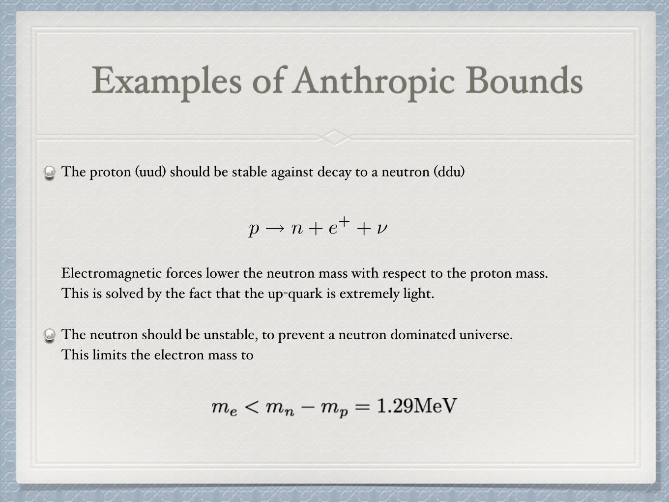
Examples of Anthropic Bounds

The proton (uud) should be stable against decay to a neutron (ddu) Electromagnetic forces lower the neutron mass with respect to the proton mass. This is solved by the fact that the up-quark is extremely light.

The neutron should be unstable, to prevent a neutron dominated universe. This limits the electron mass to

p� n + e+ + �



String TheoryLarge number of “string vacua” known since 1986. (Schellekens, 1998)Now called the “String Theory Landscape”. (Susskind, 2003; Douglas, ….)

Anthropic fine-tuningsThe Standard Model is tuned for life, suggesting that it won’t be mathematically unique.

Common senseThere is no argument for uniqueness, it is just a belief.Is all we can see all there is?

This does require physics beyond the Standard Model:A large ensemble of physically connected “vacua”.

The only known candidate is the string theory landscape.

(See Rev. Mod. Phys. 85 (2013) pp. 1491-1540 for more)

If this is true one would expect

Some gauge group, nothing mathematically special.Some choice of matter, nothing mathematically special.Some choice of parameter values, nothing mathematically special.And the whole model should extrapolate consistently to the Planck scale.

That’s exactly what we have right now!

Atomic Physics

Nuclear Physics

Hadronic Physics

The Standard Model

✗

✗

✗

✓

Running of α in Atomic Physics

Fundamental Theory

The Standard Model

New Physics





The Einstein and landscape points of view could both be correct:

But then the consistency of the SM until the Planck scale is just an accident

The Hierarchy Worry

Weak scale ⇡ 100 GeV

Planck scale ⇡ 1019GeV

+ + .....µ2�†�

The loop correction is divergent, but is assumed to be cut off at some new physics scale Λ, below or at most at the Planck scale.

If there exist heavy particles with mass M, they will contribute a correction proportional to M2 to μ2: “unnatural”

EPlanck =

r~c5G

Problem or Worry?In a finite theory, the full expression for μ2 is

But only μphys is measurable. Even if it is much smaller than each term in the sum, this has no physical consequences.

There is no hierarchy problem, just a hierarchy worry.

The Standard Model is perfectly fine as it is.

µ2phys = µ2

bare +

X

i

ai⇤2+ logs

Is the hierarchy anthropic?Weakness of gravity: brains would collapse into black holes.Maximal number of constituents:

For a “brain” with 1024 protons not to be a black hole, we need mp < 10-8 mPlanck To have stars (stellar nucleosynthesis, energy source), we need a hierarchy roughly like the one we observe. (F. Adams: “Stars In Other Universes”, arXiv:0807.3697) Agrawal et. al. (1998): Weak scale hierarchy from nuclear stability

✓mPlanck

mp

◆3

Anthropic or New Physics?

“If the electroweak symmetry breaking scale is anthropically fixed, then we can give up the decades long search for a natural solution of the hierarchy problem.”

S. Weinberg (2005)

A Derivation of the Standard Model Structure

Based on Nucl.Phys. B883 (2014) 529-580 with B. Gato Rivera

GUTs?

(3, 2,1

6) + (3⇤, 1,

1

3) + (3⇤, 1,�2

3) + (1, 2,�1

2) + (1, 1, 1)One family: +(1, 0, 0)

Charge quantization not explained by SU(3)×SU(2)×U(1)

The most popular explanation is Grand Unified Theories

One family:

(16) of SO(10)

(5

⇤) + (10) of SU(5)+ (1)

GUTs?

Higgs does not fit in a GUT representation. Breaking to SU(3) ×SU(2)×U(1) is not explained.There are alternatives, like SU(4)×U(1). Choice of representations is not explained. Choice of GUT gauge group is not explained. No evidence for coupling convergence (yet?)

1/α3

1/α2

1/α11/α1

1/α2

1/α3

SM MSSM

10logQ 10logQ0 5 10 15 0 5 10 15

Susy?

Anthropic assumptions

Sufficiently rich “atomic” physics (at least one massless photon and some (meta)stable charged particles)

Hierarchy between the scale of the atomic mass scales and gravity

We are not demanding carbon, stars, galaxies, nucleosynthesis, abundances, weak interactions(*)….

cf. Harnik, Kribs, Perez, “A universe without weak interactions”

The Hierarchy ProblemRenormalization of scalar masses

Renormalization of fermion masses

Computable statistical cost of about 10−34 for the observed hierarchy. This is the “(technical) hierarchy problem”.

Statistical cost determined by landscape distribution of λbare

µ2phys = µ2

bare +X

i

ai⇤2

�phys = �bare

X

i

bilog(⇤/Q)

!

The Hierarchy Problem

This has led to the idea that perhaps we should try to get theories with only logarithmically renormalized parameters and no quadratically renormalized scalars.

For example, the Higgs could be a composite, or the supersymmetric partner of a fermion.

All of this predicts “new physics”, which has not been found so far.

The Single Higgs Hypothesis

If we accept the current status quo, apparently nature has chosen to pay the huge price of a single scalar to create the hierarchy.

[It remains to be shown that is statistically cheaper than having fundamental Dirac particles with small masses, or than solutions to the technical hierarchy problem (susy, compositenes, ….). Requires landscape studies.]

But then this price is going to be payed only once: there should be just one Higgs.

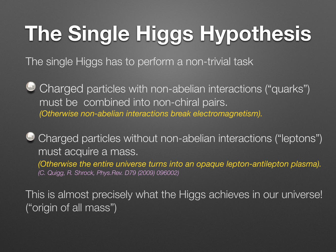
The Single Higgs HypothesisThe single Higgs has to perform a non-trivial task

Charged particles with non-abelian interactions (“quarks”) must be combined into non-chiral pairs.(Otherwise non-abelian interactions break electromagnetism).

Charged particles without non-abelian interactions (“leptons”) must acquire a mass. (Otherwise the entire universe turns into an opaque lepton-antilepton plasma). (C. Quigg, R. Shrock, Phys.Rev. D79 (2009) 096002)

This is almost precisely what the Higgs achieves in our universe! (“origin of all mass”)

String TheoryLook for theories with precisely this feature: Higgs makes chiral matter non-chiral, with massive leptons

This is very restrictive, but still has an infinite number of solutions in QFT.

The solutions can be enumerated in any theory that imposes restrictions on the choice of representation.

Here we use string theory for that purpose.

Intersecting Brane ModelsWe will assume that all matter and the Higgs bosons are massless particles in intersecting brane models.

These are characterized by higher-dimensional membranes, coinciding with our four-dimensional world, and intersecting each other in some additional, compact dimensions.

A stack of N membranes is observed as a U(N), O(N) or Sp(N) gauge group. Hence the gauge group is a product of U(N), O(N) and Sp(N) factors.

Matter is limited to a handful of choices. It originates from open strings with one end on one stack, and the other on another (or the same) stack. Massless particles (the Standard Model) originate from the brane intersections.

The low energy gauge group is assumed to come from S stacks of branes.

S=1 is easy to rule out, so we need at least S=2.

“Madrid model” (Ibañez, Marchesano, Rabadan)

Two stack modelsY = qaQa + qbQb

an anti-symmetric tensor breaks SU(N) to Sp(N) (if N is even) or Sp(N�1) (if N isodd), or to SU(N�2) ⇥ SU(2). The only way these symmetry breakings could yield aU(1) is if SU(2) is broken by means of a symmetric tensor to SO(2). But SU(2) hasno complex representations, and hence is not a suitable high-energy theory by itself; itviolates assumption 3. An adjoint representation breaks SU(N) to SU(p)⇥SU(q)⇥U(1),p + q = N . This looks promising, because at least it produces a U(1). But it is easy tosee that this can never break a chiral representation to a non-chiral one. We will discussthis in more detail for two-stack models in section 4.2.3.

4.2 Two Stack Models

The next possibility is to obtain the U(1) from two brane stacks. In this paper we willonly consider the possibility that both are unitary, and consider a general U(M)⇥U(N)two-stack model. The gauge group is SU(M)⇥ SU(N)⇥U(1)2, but anomalies (canceledby a Green-Schwarz mechanism) will leave at most one linear combination of the twoU(1)’s unbroken. We will write it as Y = qaQa + qbQb where Qa and Qb are the branecharges of the two stacks. The possibilities for chiral matter representations are then(note that adjoints are not chiral, so we do not have to consider them)

Q (M,N, qa + qb)

U (A, 1, 2qa)

D (M, 1,�qa)

S (S, 1, 2qa)

X (M,N, qa � qb) (10)

L (1, N,�qb)

T (1, S, 2qb)

E (1, A, 2qb)

where A, S denote (anti)symmetric tensors. We have given these multiplets suggestivenames referring to the Standard Model, but of course those names can correspond togenuine quarks and leptons only for M = 3 and N = 2. We will use variables Q,U,D, . . .,which can be any integer, to denote the multiplicity of these representations. If a mul-tiplicity is negative this implies a positive multiplicity for the conjugate representation.The representations themselves will be denoted asQ,U,D, . . .. We have chosen to use theanti-vectors for L and D, because then the Standard Model multiplicities will be positiveintegers. Note however that for notational convenience we have not added superscriptsto denote anti-particles. So U and D correspond to anti-quarks in the Standard Model,and L corresponds to anti-leptons.

4.2.1 Anomaly cancellation conditions

The integer multiplicities are subject to anomaly cancellation. We will denote anomaliesby a three-letter code, where ‘S’,‘W’ and ‘Y’ refer to SU(M), SU(N) and U(1), and ‘G’

22

SU(M)⇥ SU(N)⇥ U(1)

qa, qb determined by axion couplings

(We have only considered unitary branes so far)

Triangle anomaliesAnomaly Cancellation

to gravity. Hence we have anomalies of type SSS, SSY, WWW, WWY, YYY and GGY.Note that the WWW anomaly is trivial in field theory for N = 2, but in a brane modelthe requirement of tadpole cancellation still imposes it as if it were a non-abelian anomaly.Hence the anomaly contributions of vectors, symmetric and anti-symmetric tensors are 1,N + 4 and N � 4 respectively, even for N = 2 (the case N = 1 is discussed below). Wewill see however that there is a linear dependence among the six anomalies, so that theWWW anomaly is not really needed. Since we want to assume as little as possible aboutthe string theory origin of these gauge groups, it is useful to know that the anomalies weuse are really just the field-theoretic ones. Furthermore, we can use the linear dependenceto trade the awkward YYY anomaly for the much more manageable WWW anomaly.

The condition of anomaly cancellation constrains the parameters qa and qb as well asthe particle multiplicities. Note that in brane models, U(1)’s do not have to be anomalyfree, because their anomalies are canceled by the Green-Schwarz mechanism. But inthat case the corresponding gauge boson acquires a mass, and cannot be the one of theStandard Model. In brane models it may also happen that a non-anomalous U(1) acquiresa mass from mixing with axions, but this is irrelevant for our purposes. There exist modelswhere this is not the case, and those are the only ones of interest.

The anomaly cancellation conditions can be greatly simplified and brought to thefollowing form

(S + U)qa = C1

(T + E)qb = �C2

(D + 8U)qa = (4 +M)C1 +NC2 (11)

Lqb +Dqa = 0

2Eqb + 2Uqa = C1 � C2

Here qa ⌘ Mqa, qb ⌘ Nqb, C1 = �(Q�X)qb and C2 = (Q +X)qa. The Standard modelparameter values are qa = �1, qb = 1, C1 = C2 = �3, Q = U = D = L = E = 3 andS = T = X = 0, and of course satisfy these equations for M = 3, N = 2. For any M andN there are just five independent equations, demonstrating that the WWW equation isredundant even if N 6= 2.

In the derivation of these equations we used N 6= 1, M 6= 1, qa 6= 0 and qb 6= 0. IfN or M are equal to one, the SSS and WWW anomaly conditions continue to hold in abrane model, because they follow from the requirement of tadpole cancellation. If N = 1this leads to the strange results that the open string sector E contributes to anomalycancellation, even though it contains no massless states! However, the reason (11) is notnecessarily valid is that the SSY and/or WWY anomaly cancellation conditions have nomeaning anymore if M and/or N are equal to 1.

If we choose just one of the two brane stack multiplicities equal to one, we lose oneequation, but we still have five left. Since the original set of six equations has a redun-dancy, one may expect to obtain exactly the same equations, and by inspection this isindeed correct. Note that for N = 1 or M = 1 the anomaly cancellation conditions arenot just the field theoretic ones, but that there is one stringy SSS or WWW condition.

23




(S + U)qa = C1

(T + E)qb = �C2

(D + 8U)qa = (4 +M)C1 +NC2 (11)

Lqb +Dqa = 0

2Eqb + 2Uqa = C1 � C2




23




(S + U)qa = C1

(T + E)qb = �C2

(D + 8U)qa = (4 +M)C1 +NC2 (11)

Lqb +Dqa = 0

2Eqb + 2Uqa = C1 � C2




23




(S + U)qa = C1

(T + E)qb = �C2

(D + 8U)qa = (4 +M)C1 +NC2 (11)

Lqb +Dqa = 0

2Eqb + 2Uqa = C1 � C2




23

(qa=0, qb=0 treated separately)

Abelian theories

Single U(1): Higgs must break it, no electromagnetism left U(1)×U(1): No solution to anomaly cancellation for two stacks

So in two-stack models we need at least one non-abelian factor in the high-energy theory.

Strong InteractionsIt is useful to have a non-abelian factor in the low-energy theory as well, since the elementary particle charge spectrum is otherwise too poor. We need some additional interaction to bind these particles into bound states with larger charges (hadrons and nuclei in our universe).

For this to work there has to be an approximately conserved baryon number. This means that we need an SU(M) factor with M ≥ 3, and that this SU(M) factor does not become part of a larger group at the “weak” scale.

Note that SU(2) does not have baryon number, and the weak scale is near the constituent mass scale. We cannot allow baryon number to be broken at that scale.

But let’s just call this an additional assumption.

Higgs Choice

Therefore we do not consider bi-fundamental Higgses breaking both U(M) and U(N). We assume that U(N) is the broken gauge factor. Then the only Higgs choices are L,T and E.

This implies that at least one non-abelian factor is not broken by the Higgs. We take this factor to be U(M).

We will assume thatU(M) it is strongly coupled in the IR-regime and stronger than U(N).

SU(M)×U(1) (i.e. N=1)

Higgs can only break U(1), but then there is no electromagnetism.

Hence there will be a second non-abelian factor, broken by the Higgs: The “weak interactions”.

M = 3, N = 2

Higgs = LDecompose L, E, T: chiral charged leptons avoided only if

L = E, T = 0

Substitute in anomaly equation:

For M = 3, N = 2: S = 0

Sqa =

✓5�N �M

2M

◆C1

Therefore we get standard QCD without symmetric tensors.

M = 3, N = 2

Sqa =12(C2 � C1). Now we substitute this into the third equation of (11), and obtain

(5�N)C1 = MC2 (12)

For N = 2 and M = 3 this result implies that C1 = C2, and hence S = 0 (note thatthere is a second solution to the condition C2 = C1, namely M = 4, N = 1, and we willsee later what that implies). Hence to avoid chiral leptons for M = 3 we must set S = 0.Since the anti-symmetric tensor of SU(3) is an anti-triplet we are now in the desirablesituation of an SU(3) gauge group with matter only in the fundamental representation.

We will present the rest of the argument without directly using the anomaly conditions(11), because this is more insightful, and the derivation of (11) is straightforward, butrather tedious. The quark multiplets split up in the following way

Q(3, qa) +Q(3, qa + 2qb) +X(3, qa) +X(3, qa � 2qb)� U(3,�2qa)�D(3, qa) , (13)

where we have conjugated U and D in order to have only triplets. We have to pair allthese components. The first term can be paired with a component of X and with D,without any constraints on charges. But the second component can only be paired withU, since qb 6= 0. Hence if Q 6= 0, we find the relation qa+2qb = �2qa, i.e. 3qa = �2qb, andQ = U . This charge relation implies immediately that there is no partner for the secondcomponent of X, so that X must vanish. Then the first component of Q can only pairwith D, and we get D = Q. If Q = 0, we can apply the same reasoning to X, with theresult 3qa = +2qb, and X = U = D. This is just the solution with X $ Q interchangethat exists on general grounds. If Q and X both vanish there is no solution, since qa 6= 0.

All anomalies involving SU(3) already cancel, and the quark contribution to the U(1)trace anomaly cancels by itself. The relation between the charges qa and qb is the familiarone from SU(5), and so we know that all particles have their familiar charges. We choosethe Standard Model normalization conventions. We get the following equations for L, Tand E

SSY 12Q� 1

2L+ 4T = 0

GGY �L+ 3T + E = 0

YYY �34Q� 1

4L+ 3T + E = 0

which imply that L = E = Q and T = 0. Note that the SU(2) anomaly 3Q�L+6T �2Eis not really needed, and follows from the others. We do not need to check that the Higgsdoes indeed give mass to all quarks and leptons, because this is the Standard Model.

Triplet Higgs

The triplet Higgs can break SU(2)⇥U(1) in two ways [52], depending on the signs of twoterms in the Higgs potential. The Higgs vev can either take the form

hHi =✓0 00 v

◆, (14)

27

Quark sector

Q+X−D = 0 Q = U if and only if qa+2qb = −2qa

or X = U if and only if qa−2qb = −2qa

In both cases we get an SU(5) type charge relation, and hence standard charge quantization

M = 3, N = 2


(5�N)C1 = MC2 (12)






SSY 12Q� 1

2L+ 4T = 0

GGY �L+ 3T + E = 0

YYY �34Q� 1

4L+ 3T + E = 0


Triplet Higgs


hHi =✓0 00 v

◆, (14)

27

Quark sector




M = 3, N = 2


(5�N)C1 = MC2 (12)






SSY 12Q� 1

2L+ 4T = 0

GGY �L+ 3T + E = 0

YYY �34Q� 1

4L+ 3T + E = 0


Triplet Higgs


hHi =✓0 00 v

◆, (14)

27

Quark sector




M = 3, N = 2


(5�N)C1 = MC2 (12)






SSY 12Q� 1

2L+ 4T = 0

GGY �L+ 3T + E = 0

YYY �34Q� 1

4L+ 3T + E = 0


Triplet Higgs


hHi =✓0 00 v

◆, (14)

27

Quark sector




M = 3, N = 2

Hence either Q = 0 or X = 0; the choice is irrelevant.Take X = 0. Then D = Q = U, T = 0, L = E Remaining anomaly conditions: L = Q

Hence the only solution is a standard model family, occurring Q times.

The branes a and b are in principle unrelated, and can generally not be combined to a U(5) stack

M = 3, N = 2

Higgs = TThe symmetric tensor can break SU(2)×U(1) in two ways, either to U(1), in the same way as L, or to SO(2).

No allowed Higgs couplings to give mass to the charged components of L, E and T, so we must require E = L = T = 0. Then there is no solution.

Breaking to U(1) (same subgroup as L)

Breaking to SO(2)Then SO(2) must be electromagnetism. Y-charges forbid cubic T couplings, so T = 0 to avoid massless charged leptons. Quark charge pairing (to avoid chiral QED, broken by QCD) requires Q =−X. If we also require S = 0, everything vanishes.

Note: stronger dynamical assumption: S = 0

M > 3 and/or N > 2

No solution for quark pairing for M>3

Non-trivial solutions with quark and lepton pairing exist for M=3, N>2(This involves considering the most general Q+Λ, where

Q is the external U(1), and Λ a generator in the flavor group, left unbroken by dynamical symmetry breaking)

All of them satisfy standard model charge quantization, even though M+N ≠ 5

But massless charged leptons can be avoided only for N=2

Conclusions

The Standard Model is the only anthropic solution within the set of two-stack models.

Family structure (and hence family repetition), charge quantization, the weak interactions and the Higgs choice are all derived.

Standard Model charge quantization works the same way, for any value of N,even if N+3 ≠ 5.

The GUT extension offers no advantages.

Only if all couplings converge (requires susy), GUTs offer an advantage.

Anthropics

vs.

Aesthetics

Anthropics

vs.

Aesthetics

(concerns existence of observers)

Anthropics

vs.

Aesthetics

(concerns existence of observers)

(concerns happiness of observers)

Future Discoveries?

ATLAS, CMS, ALICE, LHCb, CDF, D0, TOTEM, LHCf, MoEDAL, COMPASS, NA61/SHINE, DIRAC, ALPHA, ASACUSA, AEGIS,

ATRAP, AMS, CAST, nTOF, OSQAR, XENON, LUX, DAMA, EDELWEISS, ADMX, CRESST, PICASSO, PVLAS, IAXO, REAPR,

ALPS-II, CDMS, ZEPLIN-III, WArP, COUPP, KIMS, NAIAD, ANAIS, GEODM, EURECA, SIMPLE, TEXONO, CoGeNT,

MAJORANA, XMASS, ArDM, DEAP, DarkSide, MiniCLEAN, DRIFT, NEWAGE, MIMAC, DMTPC, ANTARES, BDUNT,

BOREXINO, DAYA BAY, Double Chooz, EXO-200, HALO, IceCube, KamLAND, KM3NeT, MINERνA, MiniBooNE, MINOS, NEMO,

NOvA, OPERA, RENO, SNO+, Super-Kamiokande, GERDA, CANDLES, CUORE, NEXT-100, TROITSK, KATRIN, MARE, ECHo, Project8, Pierre Auger, PAMELA, MAGIC, HESS, DES, SDSS, Fermi-

LAT, CLIO, LIGO, GEO-600, LCGT, MiniGrail, NGO, Virgo, CryoEDM, Planck, ACBAR, AMI, AMiBA, ACT, APEX, CAPMAP,

POLARBEAR, LOFAR, VLT/UVES, Keck, ..........

Possible observations in the Singlet Era

Direct or indirect (photons from annihilation) evidence for dark matter particles. This would mean the end of the singlet era.

Evidence for a neutrino Majorana mass(neutrinoless 2β-decay)

Sterile neutrinos

Axions

Electric dipole moment of the neutron

Magnetic monopoles

Proton decay

Something totally unexpected.

An Anthropic alternative

Massless photon No massless charged leptons > 3 distinct stable atoms

Standard Model group and families are the only solutionThe Higgs choice is determined

Stacks of M and N intersecting branes.

This produces matter coupling to a gauge group SU(M) x SU(N) x U(1)

Require

B. Gato-Rivera and A. N. Schellekens, arXiv:1401.1782

Charge quantization without GUTsIn the absence of susy, GUTs only offer disadvantages

Documents

Particle Physics in the Multiverse - Nikheft58/Presentations/CSIC2015.pdf · Particle Physics in the Multiverse ... be viewed as an e↵ective theory, valid only up to Q 1. Sometimes