Embed Size (px)
Citation preview

Particle methods in CFDG.-H. Cottet
LMC-IMAG, Université Joseph Fourier
Outline:
•Basics definitions and methods for inviscid flows
•Diffusion and implicit subgrid-scale models in PM
•Regridding and multi-level PM
•Boundary conditions and interface capturing PM
Towardsmulti-physics
multi-level PM

Idea of particle methods: concentrate mass on points (particles)
Integrals become simple values, and above mass balance equationreduces to a set of differential equations
Advection equation in conservation form:
d
dtu dx
Ω(t )
∫⎛
⎝ ⎜
⎞
⎠ ⎟ + a0u dx
Ω( t )
∫ = f dxΩ(t )
∫
Conservation of mass along trajectories for Lu=f:
where Ω•
(t) = a Ω(t),t( )

Particle solution of :Lu ≡ 0
where
Fundamental examples:

Handles also Dirac functions in right hand side:
where
Lu = f
then, a particle solution reads
Here X(t;x,s) denotes the trajectory at time t originating fromx at time s
for and, for

Remarks:
Applies to linear combination of Dirac masses
Applies to vector equations
Mass of particles combine local values of u and localvolumes
What is the sense of “particle solution”?
weak solution of LU=f , that is satisfies:
u(•,t),L*ϕ(•,t)0
T
∫ dt = u0,ϕ(•,0) + f (•,t),ϕ(•,t)0
T
∫ dt
where

Consequence:
•no projection of the original equation involved•convergence based on approximation of data in appropriate space

Essential feature: transport of Dirac masses directlytranslates conservative formulation
Three classical + one less classical examples:
• Vlasov-Maxwell equations
• Gas dynamics
• Incompressible Navier-Stokes equations
• Linear elasticity

Vlasov maxwell equations
Distribution function for ions (or electrons) subject toelectric and magnetic fields
Conservation of charge:
satisfies
hence, conservative advection equation for f in velocity field U

W = (ρ,ρu,ρv,ρE) ; U = (u,v)
∂W
∂t+ div(U :W ) = Π + diffusion
Π = (0, −∇p, div(Up)) ; p = p(ρe)
Gas dynamics for compressible isentropic flows
Conservation of density, momentum and energy:

Vorticity conservation for incompressible flows
Incompressible Navier-Stokes equations in velocity-pressureformulation

Other types of particles: vorticity contours and filaments
Vorticity filament: a curve that concentrates a vortex tube
r ω
r ω
Σ1
Σ2ω • n1 dx
Σ1
∫∫ = - ω • n2 dxΣ2
∫∫
Circulation of vortex tube

Vortex filament: particle with support an oriented curve(centerline of vortex tube) and strength its circulation.
In mathematical words, filament of circulation Γ supported bycurve F parameterized by γ(ξ) :
µ,ϕ = α F
∫ ϕ γ(ξ)( ) •∂γ∂ξ
dξ
Same notions apply for contours of 2D vortex patches(method of contour dynamics): satisfies atransport-stretching equation identical to the 3D vorticityequation
∇ ×ω

In practice, filaments are tracked by a finite number of markers,and method amounts to point-particle method with stretching ofparticles implicitly accounted for by curve stretching.

So far, considered that velocity field and strain necessary to updateparticle locations and strain was given.In fact must be computed in self-consistent way from vorticity:
∇ ×u = ωω ; ∇ •u = 0
Two classical approaches:
•a completely grid-free approach, based on integral representationformulas
•an approach using grid-based Poisson solvers
First approach uses Biot-Savart law:
u = K ∗ ωω = K(x − y) × ωω(y) dy ; K = ∇(1/4π x∫ )

When ω replaced by a set of particles, velocity on each particleis expressed as
u(xp ) = αqq∑ K(xp − xq )
Two remarks:•Kernel is singular: need to mollify to avoid large values when particlesApproach•N-body problem: complexity in O(N2) if N=number of particles
Mollification is performed by convolution with cut-off with radialsymmetry and core size ε -> explicit algebraic formulasHigh order formulas obtained by imposing that cut-off shares as manymoments as possible with Dirac functionExample of formula at order 4:

Complete numerical method can be rephrased as a set of coupleddifferential equations:
Some natural conservation properties result from this formulation
dxp
dt= αq
q
∑ Kε (xp − xq )
α p
p
∑ xp (= xω(x)dx , linear impulse)∫
α p
p
∑ xp
2 (= x
2ω(x)dx , angular impulse)∫
α p
p,q
∑ αqGε (xp − xq ) (= ω(x)ω(y)Gε (x − y)dxdy , kinetic energy∫ )

O(N2) complexity can be reduce to O(NLogN) by using FastSummation Algorithms: idea is to replace kernel by algebraicexpansions:
(Greengard-Rocklin, for logarithmic kernel)
with precise estimates

Gain over direct summation can be explained on simple example
Field of M particles on N particles:• direct summation: O(MN) operations• Fast summation with p terms: O(Mp+Np)
O(Mp) calculations to compute expansion coefficients fromsources
0(Np) calculations to evaluate expansions on receivers
sour
ces receivers

Typical tree-code:
Divide recursively into boxescontaining about the same numberof particles
Upward pass:
form mulipole expansions, fromfiner to coarser level (using shifts ofpreviously computed expansions)
Downward pass:
accumulate contributions of well-separated boxes, from coarser tofiner level
At finest level, complete with directsummation of nearby particles
Still many improvements to come in 3D (parallelism ..)

Other approach for filed calculations: use an underlying Euleriangrid and grid-based Poisson solvers (Particle-In-Cell/Vortex-In-Cell methods):
•Project particle strength on grid points•Use a Poisson solver on that grid, and differentiate on the grid to get gridfield values•Interpolate back fields on particlesDrawbacks:•against Lagrangian features of particles (and possible loss ofinformation in grid-particle interpolations)
•require far-field artificial boundary conditions
Advantage:Cheap (for relatively simple geometries)

Comparison of CPU times for velocity evaluations in 3D
(Krasny tree-code vs VIC with Fishpack and 64 points interpolation formulas)
directsummation
Treecode
VIC1
VIC3
VIC2
VIC1: cartesian gridwith 100% particles
VIC2: polar grid with65% particles
VIC3: polar grid with25% particles

Conclusion: choice of solver depends on how localized vorticityis in the computational box needed:
Flow past a sphere: grid-free calculation (Ploumehans et al.)
Flow past a cylinder:VIC calculation (C.-Poncet)
About 600,000 particles,Total cpu is 200 hours on 32 HP processors
Cylindrical grid: 256x128x128 in a domain filled with 25% particlesCPU time: 3mn/RK4 iteration on alphasingle processor, 3hours/shedding cycle
4π × 2π × 2π

Possible to combine both approaches (grid-free and particle-in-cell)through domain decomposition approaches: far-field by grid-free,“boundary layer” by PIC.
Other issue related to velocity evaluations: time-stepping to pushparticles and update strengths
In general RK2 or RK4
Linear stability only requires particle not to cross each other
(no conventional CFL type condition):
∆t ≤C
∇u∞
CPU savings depend on particular flow

1. Handling diffusion in particle methods2. Understanding how particle methods work at
sub-grid level3. Regridding of particles4. Towards adaptive multi-level particle methods
Lecture 2

Focus on heat equation in free space
Explicit exact solution with integral formula
Where Gaussian kernel given in 2D by

When field given on particles, obtain superposition of gaussian blobs
First method: random walk method (Chorin 70s)
Sample these blobs by particles with appropriate density
1 particle per blob -> random walk of each particle after advection step
Convergence relies on large number laws

Formula for n steps of random walks for N particles
where
And u’s and θ’s are independent random variables with uniformdensity
For advection-diffusion problems: similar formula alternatingparticles advection and random walks
Can be interpreted as quadrature of exact solution (repeatedconvolution with Gaussian kernels) on N random points over a spaceon dimension n -> convergence ratePhysically and mathematically appealing, but not very accurate
1/ N

Particle resampling schemes
Idea: evaluate gaussians on particles and use these values to update their weigths
Can be interpreted by rewriting diffusion as an integral operator

Theorem: if kernel η satisfies the following moment properties:
then
In practice, any positive, compacted supported, radiallysymmetric function, after proper normalization, will do it

Resulting particle scheme
Here, we distinguish local values and volumes that make theparticles strengths
Not constrained with time-stepping, can be high order
Slightly more expensive than random walk

This approach extends to anistropic diffusion
with (for instance)

Implicit subgrid-scale models in particle methods
Focus on 3D Euler equations (inviscid flows) in vorticity formulation
Particle solution given by
where is a mollified velocity field. u
weak solution to

Molified particles (blobs) thus satisfy
This is an averaged Euler equationsThis means that the particle method is achieving some subgrid scale(implicit) modelThe transfer from larges scales to samll scales can be illustrated bythe following sketch

More precise analysis needed to understand enstrophy transfersFor simplicity, consider 2D case and start from
Where ωε = ω = ω ∗ ςε

First term is a drift which does not contribute to enstrophy balance
Second term can be rewritten after Taylor expansions as
For symmetry reasons, cross terms disappear and we are left with
with
In other words, «equivalent» equation for large scales (blobs) is Euler + diffusion with anisotropic eddy viscosity

Back to the enstrophy balance: compute (drop ε for simplicity) ωEdx∫
First term vanishes (div u = 0) and for second term write
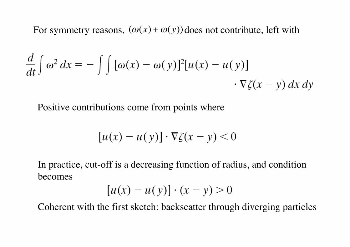
For symmetry reasons, does not contribute, left with(ω(x) + ω(y))
Positive contributions come from points where
In practice, cut-off is a decreasing function of radius, and condition becomes
Coherent with the first sketch: backscatter through diverging particles

In practice, codes have always trouble to handle backscatter: Need to compensate ,at least partially
Two ways to prevent excess backscatter in a particle code:• remesh particles or• use above calculations to tune the proper diffusion model:
Non-linear diffusion, acting only on directions of diverging particles(positive eigenvalues of strain tensor)
ς(x) = f ( x )where

Illustration: 2D decaying turbulence:correlations between eddy viscosity and high strain zones
T=1
T=2
vorticity viscosity

Comparison of pure Euler simulation (with backscatter) and eddy-viscosity correction
With correction
Pure Euler
T=1 T=2

Rk: More traditional way to cope with small scale: hairpin removal (Chorin, Leonard)
Conclusion:
•particles give a nice insight into subgrid level
•differences and links with «conventional»subgridscale modeling in grid-based methods
•numerical analysis allows to control excessbackscatter

Adaptive, multilevel particle methods
First remark: particles methods are naturally adaptivefor 2 reasons:•Particles in general follow zones of interest, which may occupy onlya small areaEx: electron beams in plasma, shear layers in flows
•If connectivity between particle can be tracked, there are easy waysto «refine» locallyEx: vortex sheet calculations of Krasny in 2d and Meiburg in 3D.

Krasny’s 2D vortex sheet calculations
Time evolution of the vortex sheet Close view of the spiral
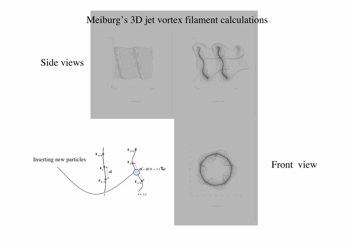
Side views
Front viewInserting new particles
Meiburg’s 3D jet vortex filament calculations

However these techniques do not apply with more complex vorticity generation and/or in presence of diffusion

Accuracy requires frequent regriddingwith high order formulas
conservation of f dx ,∫ xf dx,∫ x2 f dx∫
M'4 (x) =
⎧
⎨ ⎪
⎩ ⎪
1− 5x2 / 2 + 3 x3
/ 2 if 0 ≤ x ≤ 1
(2 − x )2(1 − x ) / 2 if 1 ≤ x ≤ 2
0 if 2 ≤ x
Λ2 (x) =
⎧
⎨ ⎪
⎩ ⎪
1 − x2 if 0 ≤ x ≤1 / 2
(1 − x )(2 − x ) / 2 if 1/ 2 ≤ x ≤ 3 / 2
0 if 3/ 2 ≤ x
«classical» interpolation formulas

Error curves
random init quiet start init
quiet start initwith remeshing
Typical example showing importance of regridding: circular patch withhigh strain

Regridding can also be used as a way to adapt particlesto the flow topology -> variable-size particles
three different approaches:
•Regridding into variable-sized particles via global mappings•Regridding via local mappings•Regridding onto piecewise uniform particles

Physical space
Mapped space
x = F( ˆ x );G = F −1
xp,vp ,ω p
ˆ x p, ˆ v p , ˆ ω p

1) Mollified particles (for field evaluation) with blob size
εp = ˆ ε J−1(xp )
2) Diffusion in mapped coordinates:
Can be written in divergence form, using the fact that
/

Using particle diffusion formulas for anisotropic diffusion we obtain

->
Remark: conservative in physical variables

Example: rebound of a dipole with exponentially stretched particle

Coarse to fine grid
T=0 T=2
T=2T=2 fine gridCoarse grid:wrong result

Flow around 2D cylinder - Variable-size particles

Rather flexible (about 10 lines of codes more than in the «uniformblob» case) but global mapping not always known analytically
Other option is to combine several local mappings (domaindecomposition approach)
Example of 2 obstacles in a flow:3 mappings: 1 around each obstacle, with refinement in theboundary layer, 1 in between with uniform blobs.


Based on overlapping of domains:
•At beginning of step, in the buffer zone:
Particles 1 and 2 are remeshed ontoparticles of type 3 (with cartesianmapping)Particles of type 3 remeshed ontoparticles of type 1 and 2 (with polarmapping)
•Then particles are advanced andexchange vorticty in each subdomain
Solution is correct except near theboundaries of overlapping zoneOverlapping zone must be big enough tocontain trajectories for one time-step anddiffusion stencil (a few grid points)
Regridding provides interpolation needed to exchangeinformation between non-conforming subdomains

Method can be extended to Adaptive Mesh Refinement:•Define zones with hierarchical grid levels, with overlapping, based on velocity gradients•Use regridding in overlapping to exchange information between gridsat different levels


Conclusion: particles have an unusual flexibility to dealwith very non-conforming domain decomposition (foradvection dominated problems) that allow to adapt locallygrid-resolution.
Major achievements of adaptive particle methods are inparticular case (sheets, filaments).
Many open pending applications of more general adaptiveschemes ..

Intermezzo: dipole ring interaction•2D case at moderate Reynolds number (Re=3,200)•3D case: inclined ring impinging on a wall (Re=1,400)

Systematic investigation of truncation error (in particular remeshing) In DNS of Isotropic homogeneous turbulence
I. DNS regime (1283 calculations)II LES regime (Comte-Bellot experiment, 323 claculations)

Statistics: comparisons with spectral reference results

Coherent structures at t=5
Spectral code VIC code

Decaying turbulence in LES regime(Comte-Bellot experiment):
comparison with spectral method with Smagorinsky model

Boundary conditions in vortex methodsin the spirit of immersed boundary
techniques

Why immersed boundaries for flows aroundbodies?
For more complex geometries, building the meshcan double the time of a full simulation
Even for simple geometries, body-fitted meshes are notstraightforward: examples for turbulent cylinder wakessimulations
C-mesh (Mittal,Moin) Spectral element (Henderson)

Immersed boundaries for flows aroundsolid boundaries: general idea
• Deal with boundaries as forcing terms in thedynamics, rather than using a body-fitted grid
• Budget accuracy vs flexibility ?
• Possible with finite-difference methods (Fadlun et al.,
JCP 2000) but particles have something special, inparticular for moving interfaces.

Two levels of boundary conditions:
1. velocity from vorticity
2. vorticity b.c. in the Navier Stokes equation
(1) ∇ × u = ω , ∇ • u = 0 Ω
u• n = 0 ∂Ω
⎧ ⎨ ⎩
(2)
∂ω∂t
+ ...= 0 Ω
∂ω∂n = g ∂Ω
⎧
⎨ ⎪
⎩ ⎪
g s.t. u•τ = 0 on ∂Ω

(1) Velocity calculation in a vortex code
where
−∆Ψ = ω
∇ • Ψ = 0
−∆Φ = 0
∂Φ
∂n= −(∇ × Ψ) • n
u = ∇ × Ψ + ∇Φ Helmholtzdecomposition
Remark: decouples b.c. and divergence-freeconstraint on stream-function

Velocity calculation (2D case)
∇ × u = ω
∇ • u = 0
u • n = 0
u(x) = u∞ + K(∫ x − y)ω(y)dy + K(x − y)q(y)dy∫
Biot-Savart law:
Potential q determined by anintegral equation on the boundary
⇒
Conclusion: no-through flow b.c. satisfiedexactly even if particles in fluid do not matchboundary discretization points

Bad news: Elliptic problem with boundary condition on immersedboundary not very well behaved (see fictitious domain methods)
∇ • u = 0
u • τ |∂Ω = 0⇒ u • n = O(h 2 ) at grid points near boundary
BUT
Solution adopted:1) tag grid-points near boundary
2) solve the linear system (GMRES type method):
ξΜ → ∆Φ = ξ →∂Φ
∂n M
= 0
Where M are the grid cells which intersect the boundary
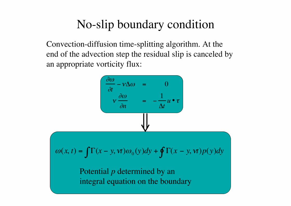
No-slip boundary condition
Convection-diffusion time-splitting algorithm. At theend of the advection step the residual slip is canceled byan appropriate vorticity flux:
∂ω∂t
−ν∆ω = 0
ν∂ω∂n
= −1
∆tu •τ⇒
ω(x, t) = Γ(∫ x − y, νt)ω0 (y)dy + Γ(x − y, νt)p(y)dy∫
Potential p determined by anintegral equation on the boundary
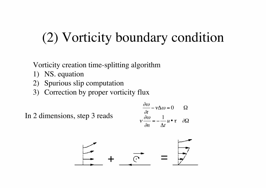
(2) Vorticity boundary condition
Vorticity creation time-splitting algorithm1) NS. equation2) Spurious slip computation3) Correction by proper vorticity flux
∂ω∂t
−ν∆ω = 0 Ω
ν∂ω∂n
= −1
∆tu•τ ∂Ω
In 2 dimensions, step 3 reads

In 3D, need boundary conditions for 3 vorticity components
+
=
After advection step computation of slip
∂ ω∂
ν ω δ
ω
ν∂ ω∂
∂∂
∂ δ
ν∂ ω∂
κω∂∂
∂ δ
ω ∂ δ
θ
θθ
tt t t
t
n
u
tt t t
n
u
tt t t
t t t
z
z
r
− = × +
=
= − × +
+⎛
⎝⎜
⎞
⎠⎟ = − × +
= × +
⎧
⎨
⎪⎪⎪⎪⎪⎪
⎩
⎪⎪⎪⎪⎪⎪
∆ Ω
Ω
Ω
Ω
Ω
0
0
0
0 0
0
0 0
0 0
0 0
sur
sur
sur
sur
sur
] , [
( )
] , [
] , [
] , [
Vorticity flux onto flow particles

In practice, the Neumann b.c. are implemented by integralformulas:
This algorithm is, by itself, an immersed boundarymethod
ω'= ω + Γ(x − y,ν∆t)g(y)dy∂Ω
∫
Rk: the flux formula alsocorrects the spurious vorticityfluxes induced by regridding ona cartesian grid

Test case: Collision ring-cylinder on a cartesian mesh


![CFD model of a fluidized bed chemical · Interconnected multi-phase CFD chemical looping model Glt m s,ox m air exhaust General parame ers Time step Δt [s] 0.0002 Mean particle diameter](https://img.dokumen.tips/doc/110x75/6011be0f8baee42d485d50cb/cfd-model-of-a-fluidized-bed-chemical-interconnected-multi-phase-cfd-chemical-looping.jpg)


