Cop

yrig

ht ©

201

4 U

nive

rsity

of C

ambr

idge

. Not

to b

e qu

oted

or

repr

oduc

ed w

ithou

t per

mis

sion

.

Partial Differential Equations

David Stuartdmas2@cam.ac.uk

Books

In addition to the sets of lecture notes written by previous lecturers ([1, 2]) whichare still useful, the books [4, 3] are very good for the PDE topics in the course,and go well beyond the course also. If you want to read more on distributions [6]is most relevant. Also [7, 8] are useful; the books [5, 9] are more advanced, butmay be helpful.

References

[1] T.W. Korner, Cambridge Lecture notes on PDE, available athttps://www.dpmms.cam.ac.uk/ twk

[2] M. Joshi and A. Wassermann, Cambridge Lecture notes on PDE,available athttp://www.damtp.cam.ac.uk/user/dmas2

[3] G.B. Folland, Introduction to Partial Differential Equations, Princeton 1995,QA 374 F6

[4] L.C. Evans, Partial Differential Equations,AMS Graduate Studies in Mathe-matics Vol 19, QA377.E93 1990

[5] H. Brezis, Functional Analysis, Sobolev Spaces and Partial Differential Equa-tions, Springer, New York 2011 QA320 .B74 2011

[6] F.G. Friedlander, Introduction to the Theory of Distributions, CUP 1982,QA324

[7] F. John, Partial Differential Equations, Springer-Verlag 1982, QA1.A647

[8] Rafael Jos Iorio and Valria de Magalhes Iorio, Fourier analysis and partialdifferential equations CUP 2001, QA403.5 .I57 2001

[9] M.E. Taylor, Partial Differential Equations,Vols I-IIISpringer 96, QA1.A647

Cop

yrig

ht ©

201

4 U

nive

rsity

of C

ambr

idge

. Not

to b

e qu

oted

or

repr

oduc

ed w

ithou

t per

mis

sion

.

1 Introduction

1.1 Notation

We write partial derivatives as ∂t = ∂∂t

, ∂j = ∂∂xj

etc and also use suffix on a function

to indicate partial differentiation: ut = ∂tu etc. A general kth order linear partialdifferential operator (pdo) acting on functions u = u(x1, . . . xn) is written:

P =∑

|α≤k

aα∂αu . (1.1.1)

Here α = (α1, . . . αn) ∈ Zn+ is a multi-index of order |α| =

∑αj and

∂α =∏

∂αj

j , xα =∏

xαj

j . (1.1.2)

For a multi-index we define the factorial α! =∏

αj!. For (real or complex) con-stants aα the formula (1.1.1) defines a constant coefficient linear pdo of order k.(Of course assume always that at least one of the aα with |α| = k is non-zero sothat it is genuinely of order k.) If the coefficients depend on x it is a variablecoefficient linear pdo. The word linear means that

P (c1u1 + c2u2) = c1Pu1 + c2Pu2 (1.1.3)

holds for P applied to Ck functions u1, u2 and arbitrary constants c1, c2.

1.2 Basic definitions

If the coefficients depend on the partial derivatives of a function of order strictlyless than k the operator

u 7→ Pu =∑

|α≤k

aα(x, ∂βu|β|<k) ∂αu (1.2.1)

is called quasi-linear and (1.1.3) no longer holds. The corresponding equationPu = f for f = f(x) is a quasi-linear partial differential equation (pde). In suchequations the partial derivatives of highest order - which are often most important- occur linearly. If the coefficients of the partial derivatives of highest order in aquasi-linear operator P depend only on x (not on u or its derivatives) the equationis called semi-linear. If the partial derivatives of highest order appear nonlinearlythe equation is called fully nonlinear; such a general pde of order k may be written

F (x, ∂αu|α|≤k) = 0 . (1.2.2)

Definition 1.2.1 A classical solution of the pde (1.2.2) on an open set Ω ⊂ Rn is

a function u ∈ Ck(Ω) which is such that F (x, ∂αu(x)|α|≤k) = 0 for all x ∈ Ω .

2

Cop

yrig

ht ©

201

4 U

nive

rsity

of C

ambr

idge

. Not

to b

e qu

oted

or

repr

oduc

ed w

ithou

t per

mis

sion

.

Classical solutions do not always exist and we will define generalized solutionslater in the course. The most general existence theorem for classical solutions is theCauchy-Kovalevskaya theorem, to state which we need the following definitions:

Definition 1.2.2 Given an operator (1.1.1) we define

• Pprincipal =∑

|α=k aα∂αu , (principal part)

• p =∑

|α≤k aα(iξ)α , ξ ∈ Rn , (total symbol)

• σ =∑

|α=k aα(iξ)α , ξ ∈ Rn , (principal symbol)

• Charx(P ) = ξ ∈ Rn : σ(x, ξ) = 0 , (the set of characteristic vectors at x)

• Char(P ) = (x, ξ) : σ(x, ξ) = 0 = ∪xCharx(P ) , (characteristic variety) .

Clearly σ, p depend on (x, ξ) ∈ R2n for variable coefficient linear operators, but are

independent of x in the constant coefficient case. For quasi-linear operators wemake these definitions by substituting in u(x) into the coefficients, so that p, σ and(also the definition of characteristic vector) depend on this u(x).

Definition 1.2.3 The operator (1.1.1) is elliptic at x (resp. everywhere) if theprincipal symbol is non-zero for non-zero ξ at x (resp. everywhere). (Again thedefinition of ellipticity in the quasi-linear case depends upon the function u(x) inthe coefficients.)

The elliptic operators are an important class of operators, and there is a well-developed theory for elliptic equations Pu = f . Other important classes of opera-tors are the parabolic and hyperbolic operators: see the introductions to sections4 and 5 for defintions of classes of parabolic and hyperbolic operators of secondorder.

1.3 The Cauchy-Kovalevskaya theorem

The Cauchy problem is the problem of showing that for a given pde and givendata on a hypersurface S ⊂ R

n there is a unique solution of the pde which agreeswith the data on S. This is a generalization of the initial value problem forordinary differential equations, and by analogy the appropriate data to be givenon S consists of u and its normal derivatives up to order k−1. A crucial conditionis the following:

Definition 1.3.1 A hypersurface S is non-characteristic at a point x if its normalvector n(x) is non-characteristic, i.e. σ(x, n(x)) 6= 0. We say that S is non-characteristic if it is non-characteristic for all x ∈ S.)

3

Cop

yrig

ht ©

201

4 U

nive

rsity

of C

ambr

idge

. Not

to b

e qu

oted

or

repr

oduc

ed w

ithou

t per

mis

sion

.

Again for quasi-linear operators it is necessary to substitute u(x) to make sense ofthis definition, so that whether or not a hypersurface is non-characteristic dependson u(x), which amounts to saying it depends on the data which are given on S.

Theorem 1.3.2 (Cauchy-Kovalevskaya theorem) In the real analytic case thereis a local solution to the Cauchy problem for a quasi-linear pde in a neighbourhoodof a point as long as the hypersurface is non-characteristic at that point.

This becomes clearer with a suitable choice of coordinates which emphasizesthe analogy with ordinary differential equations: let the hypersurface be the levelset xn = t = 0 and let x = (x1, . . . xn−1) be the remaining n− 1 coordinates. Thena quasi-linear P takes the form

Pu = a0k∂kt +

∑

|α|+j≤k,j<k

ajα∂jt ∂

αu (1.3.1)

with the coefficients depending on derivatives of order < k, as well as on (x, t).Since the normal vector to t = 0 is n = (0, 0, . . . 0, 1) ∈ R

n the non-characteristiccondition is just a0k 6= 0, and ensures that the quasi-linear equation Pu = f canbe solved for ∂k

t u in terms of ∂jt ∂

αu|α|+j≤k,j<k to yield an equation of the form:

∂kt u = G(x, t, ∂j

t ∂αu|α|+j≤k,j<k) (1.3.2)

to be solved with data

u(x, 0) = φ0(x), ∂tu(x, 0) = φ1(x) . . . ∂k−1t u(x, 0) = φk−1(x) . (1.3.3)

Notice that these data determine, for all j < k, the derivatives

∂jt ∂

αu(x, 0) = ∂αφj(x) , (1.3.4)

(i.e. those involving fewer than k normal derivatives ∂t) on the initial hypersurface.

Theorem 1.3.3 Assume that φ0, . . . φk−1 are all real analytic functions in someneighbourhood of a point x0 and that G is a real analytic function of its argumentsin a neighbourhood of (x0, 0, ∂αφj(x0)|α|+j≤k,j<k). Then there exists a unique realanalytic function which satisfies (1.3.3)-(1.3.2) in some neighbourhood of the pointx0.

Notice that the non-characteristic condition ensures that the kth normal derivative∂k

t u(x, 0) is determined by the data through the equation. Differentiation of (1.3.2)gives further relations which can be shown to determine all derivatives of thesolution at t = 0, and the theorem can be proved by showing that the resultingTaylor series defines a real-analytic solution of the equation. Read section 1C ofthe book of Folland for the full proof.

4

Cop

yrig

ht ©

201

4 U

nive

rsity

of C

ambr

idge

. Not

to b

e qu

oted

or

repr

oduc

ed w

ithou

t per

mis

sion

.

In the case of first order equations with real coefficients the method of character-istics gives an alternative method of attack which does not require real analyticity.In this case we consider a pde of the form

n∑

j=1

aj(x, u)∂ju = b(x, u) (1.3.5)

with datau(x) = φ(x) , x ∈ S (1.3.6)

where S ⊂ Rn is a hypersurface, given in paramteric form as xj = gj(σ) , σ =

(σ1, . . . σn−1) ∈ Rn−1. (Think of S = xn = 0 parametrized by g(σ1, . . . σn−1) =

(σ1, . . . σn−1, 0).)

Theorem 1.3.4 Let S be a C1 hypersurface, and assume that the aj, b, φ are allC1 functions. Assume the non-characteristic condition:

Σnj=1aj(x0, φ(x0))nj(x0) 6= 0

holds at a point x0 ∈ S. Then there is an open set O containing x0 in which thereexists a unique C1 solution of (1.3.5) which also satisfies (1.3.6) at all x ∈ O∩S.If the non-characteristic condition holds at all points of S, then there is a uniquesolution of (1.3.5)-(1.3.6) in an open neighbourhood of S.

This is proved by considering the characteristic curves which are obtained byintegrating the system of n+1 characteristic ordinary differential equations (ode):

dxj

ds= aj(x, z) ,

dz

ds= b(x, z) (1.3.7)

with data xj(σ, 0) = gj(σ), z(σ, 0) = φ(g(σ)); let (X(σ, s), Z(σ, s)) ∈ Rn × R be

this solution. Now compute the Jacobian matrix of the mapping (σ, s) 7→ X(σ, s)at the point (σ, 0): it is the n × n matrix whose columns are ∂σj

gn−1j=1 and the

vector a = (a1, . . . an), evaluated at x = g(σ), z = φ(g(σ)). The non-characteristiccondition implies that this matrix is invertible (a linear bijection) and hence, viathe inverse function theorem, that the “restricted flow map” which takes (σ, s) 7→X(σ, s) = x is locally invertible, with inverse σj = Σj(x), s = S(x) and thisallows one to recover the solution as u(x) = Z(Σ(x), S(x)). This just means wehave found a locally unique characteristic curve passing through x, and have thenfound u(x) by tracing its value back along the curve to a point g(Σ(x)) on theinitial hypersurface.

1.4 Some worked problems

1. Consider the two-dimensional domain

G := (x, y) | R21 < x2 + y2 < R2

2,

5

Cop

yrig

ht ©

201

4 U

nive

rsity

of C

ambr

idge

. Not

to b

e qu

oted

or

repr

oduc

ed w

ithou

t per

mis

sion

.

where 0 < R1 < R2 < ∞. Solve the Dirichlet boundary value problem for the Laplaceequation

∆u = 0 in G,

u = u1(ϕ), r = R1,

u = u2(ϕ), r = R2,

where (r, ϕ) are polar coordinates. Assume that u1, u2 are smooth 2π-periodic functionson the real line.

Discuss the convergence properties of the series so obtained.

[Hint: Use separation of variables in polar coordinates (u = R(r)Φ(ϕ)), with perodicboundary conditions for the function Φ of the angle variable. Use an ansatz of the formR(r) = rα for the radial function.]

Answer As the hint suggests, we use radial coordinates and transform the Laplacian. Usingthis, our PDE becomes

urr +1

rur +

1

r2uϕϕ = 0.

Using separation of variables as the hint suggests yields

R′′Φ +1

rR′Φ +

1

r2RΦ′′ = 0

We multiply this equation by r2

RΦ and rearrange to obtain an equality between an expres-sion which depends only on r and an expression which depends only on ϕ. This impliesthat the two equations are equal to a constant (denoted λ2):

r2R′′(r) + rR′(r)

R(r)=

−Φ′′(ϕ)

Φ= λ2

We require a 2π periodicity for each value of the radial coordinate, so we require that Φbe 2π periodic, and thus obtain:

Φ(ϕ) = A sin(λϕ) + B cos(λϕ),

with positve constants A, B. Since we assume the solution to be 2π-periodic it followsthat λ must be an integer, and w.l.o.g. λ is non-negative.

For the other equation we use the Ansatz R(r) = rα and obtain

α(α − 1)rα + αrα − λ2rα = 0

and thusα = ±λ.

Therefore

R(r) = Crλ + Dr−λ, if λ > 0

and by considering the case λ = 0 separately

R(r) = E + F ln(r), if λ = 0.

6

Cop

yrig

ht ©

201

4 U

nive

rsity

of C

ambr

idge

. Not

to b

e qu

oted

or

repr

oduc

ed w

ithou

t per

mis

sion

.

As the equation is linear, the most general solution is

u(r, ϕ) =

∞∑

λ=1

(Aλrλ + Bλr−λ) sin(λϕ) + (Cλrλ + Dλr−λ) cos(λϕ)

+ E0 + F0 ln(r)

To account for the boundary conditions, we expand u1 and u2 as Fourier series:

u1(ϕ) =a0

2+

∞∑

λ=1

aλ sin(λϕ) + bλ cos(λϕ),

u2(ϕ) =c0

2+

∞∑

λ=1

cλ sin(λϕ) + dλ cos(λϕ).

(This is possible by the assumptions on u1,2.) To enforce

u(R1, ϕ) = u1(ϕ), u(R2, ϕ) = u2(ϕ)

comparison of the coefficients leads to

AλRλ1 + BλR−λ

1 = aλ, AλRλ2 + BλR−λ

2 = cλ,

CλRλ1 + DλR−λ

1 = bλ, CλRλ2 + DλR−λ

2 = dλ

and

E0 + F0 ln(R1) =a0

2,

E0 + F0 ln(R2) =c0

2.

The first two equations result in

Aλ =Rλ

1aλ − Rλ2 cλ

R2λ1 − R2λ

2

, Bλ =R−λ

1 aλ − R−λ2 cλ

R−2λ1 − R−2λ

2

,

and

Cλ =Rλ

1 bλ − Rλ2dλ

R2λ1 − R2λ

2

, Dλ =R−λ

1 bλ − R−λ2 dλ

R−2λ1 − R−2λ

2

.

From the last equation we obtain

E0 =a0 ln(R2) − c0 ln(R1)

2(ln(R2) − ln(R1)), F0 =

c0 − a0

2(ln(R2) − ln(R1)).

Since the u1,2 are smooth and periodic, their Fourier coeficients are rapidly decreasing,i.e.

supλ∈N

λN (|aλ| + |bλ| + |cλ| + |dλ|) < ∞

for any positive N . Now let ρ = R1/R2 = (R2/R1)−1 ∈ (0, 1), then the above formulae

can be written as

Aλ = R−λ2

cλ − ρλaλ

1 − ρ2λ, Bλ = Rλ

1

aλ − ρλcλ

1 − ρ2λ,

7

Cop

yrig

ht ©

201

4 U

nive

rsity

of C

ambr

idge

. Not

to b

e qu

oted

or

repr

oduc

ed w

ithou

t per

mis

sion

.

and

Cλ = R−λ2

dλ − ρλbλ

1 − ρ2λ, Dλ = Rλ

1

bλ − ρλdλ

1 − ρ2λ.

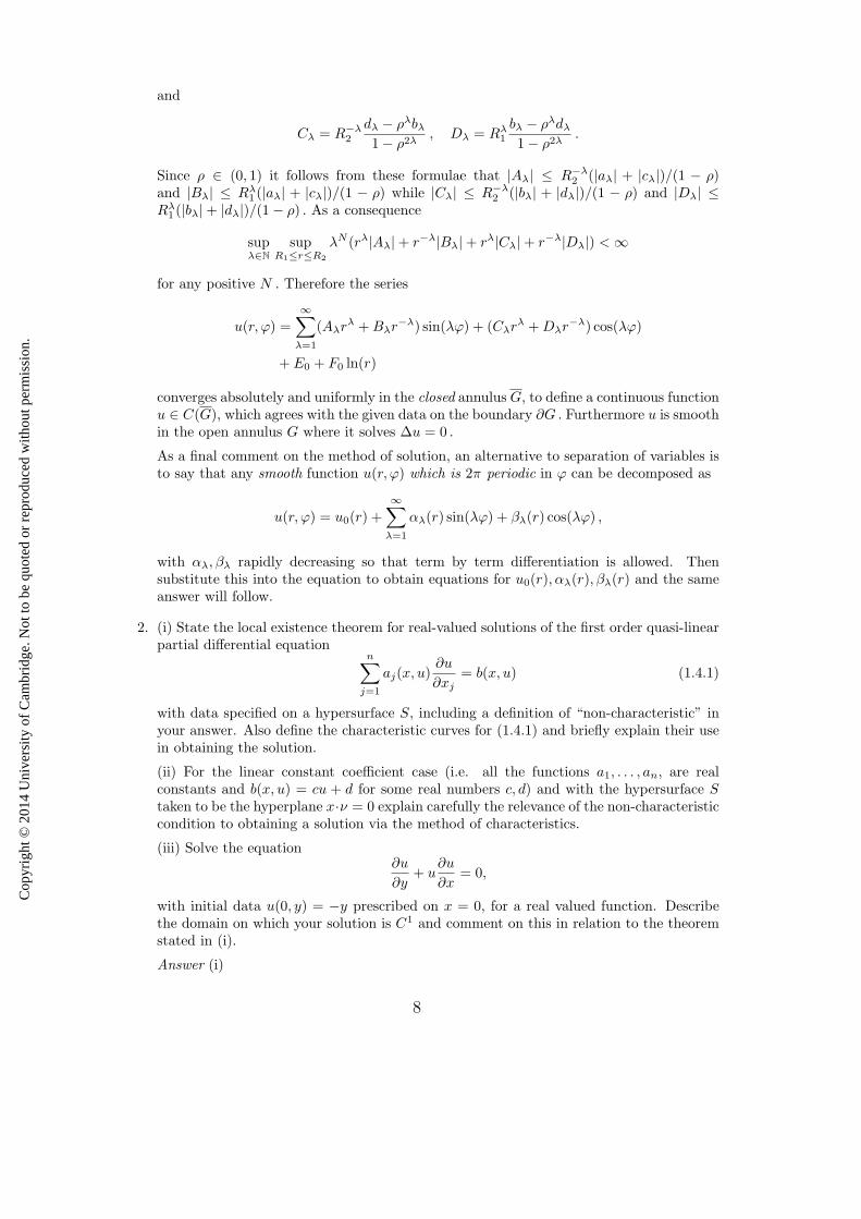
Since ρ ∈ (0, 1) it follows from these formulae that |Aλ| ≤ R−λ2 (|aλ| + |cλ|)/(1 − ρ)

and |Bλ| ≤ Rλ1 (|aλ| + |cλ|)/(1 − ρ) while |Cλ| ≤ R−λ

2 (|bλ| + |dλ|)/(1 − ρ) and |Dλ| ≤Rλ

1 (|bλ| + |dλ|)/(1 − ρ) . As a consequence

supλ∈N

supR1≤r≤R2

λN (rλ|Aλ| + r−λ|Bλ| + rλ|Cλ| + r−λ|Dλ|) < ∞

for any positive N . Therefore the series

u(r, ϕ) =

∞∑

λ=1

(Aλrλ + Bλr−λ) sin(λϕ) + (Cλrλ + Dλr−λ) cos(λϕ)

+ E0 + F0 ln(r)

converges absolutely and uniformly in the closed annulus G, to define a continuous functionu ∈ C(G), which agrees with the given data on the boundary ∂G . Furthermore u is smoothin the open annulus G where it solves ∆u = 0 .

As a final comment on the method of solution, an alternative to separation of variables isto say that any smooth function u(r, ϕ) which is 2π periodic in ϕ can be decomposed as

u(r, ϕ) = u0(r) +

∞∑

λ=1

αλ(r) sin(λϕ) + βλ(r) cos(λϕ) ,

with αλ, βλ rapidly decreasing so that term by term differentiation is allowed. Thensubstitute this into the equation to obtain equations for u0(r), αλ(r), βλ(r) and the sameanswer will follow.

2. (i) State the local existence theorem for real-valued solutions of the first order quasi-linearpartial differential equation

n∑

j=1

aj(x, u)∂u

∂xj= b(x, u) (1.4.1)

with data specified on a hypersurface S, including a definition of “non-characteristic” inyour answer. Also define the characteristic curves for (1.4.1) and briefly explain their usein obtaining the solution.

(ii) For the linear constant coefficient case (i.e. all the functions a1, . . . , an, are realconstants and b(x, u) = cu + d for some real numbers c, d) and with the hypersurface Staken to be the hyperplane x·ν = 0 explain carefully the relevance of the non-characteristiccondition to obtaining a solution via the method of characteristics.

(iii) Solve the equation∂u

∂y+ u

∂u

∂x= 0,

with initial data u(0, y) = −y prescribed on x = 0, for a real valued function. Describethe domain on which your solution is C1 and comment on this in relation to the theoremstated in (i).

Answer (i)

8

Cop

yrig

ht ©

201

4 U

nive

rsity

of C

ambr

idge

. Not

to b

e qu

oted

or

repr

oduc

ed w

ithou

t per

mis

sion

.

Theorem 1.4.1 Let S be a C1 hypersurface, and assume that the aj , b, φ are all C1

functions. Assume the non-characteristic condition:

Σnj=1aj(x0, φ(x0))nj(x0) 6= 0

holds at a point x0 ∈ S. Then there is an open set O containing x0 in which there existsa unique C1 solution of (1.4.1) which also satisfies

u(x) = φ(x) , x ∈ S ∩ O . (1.4.2)

If the non-characteristic condition holds at all points of S, then there is a unique solutionof (1.4.1)-(1.3.6) in an open neighbourhood of S.

The characteristic curves are obtained as the x component of the integral curves of thecharacteristic ode:

dxj

ds= aj(x, z) ,

dz

ds= b(x, z) (1.4.3)

with data xj(σ, 0) = gj(σ), z(σ, 0) = φ(g(σ)); let (X(σ, s), Z(σ, s)) ∈ Rn × R be this

solution. The characteristic curves starting at g(σ) are the curves s 7→ X(σ, s). They areuseful because the non-characteristic condition implies (via the inverse function theorem)that the “restricted flow map” which takes (σ, s) 7→ X(σ, s) = x is locally invertible, withinverse σj = Σj(x), s = S(x) and this allows one to obtain the solution by tracing alongthe characteristic curve using the z component of the characteristic ode above. This givesthe final formula: u(x) = Z(Σ(x), S(x)).

(ii) In the linear constant coefficient case the non-characteristic condition reads a · ν 6= 0,and the characteristic curves are lines with tangent vector a = (a1, . . . an), obtained byintegrating the characteristic ode:

dxj

ds= aj ,

dz

ds= b(x, z) = cz + d , (1.4.4)

and taking the “x component”. The flow map is the smooth function R×Rn → R

n givenby

Φ(s, x) = x + sa,

i.e. the solution of the characteristic ode starting at x . Parametrize the initial hyperplaneas x =

∑n−1j=1 σjγj , where the γj ∈ R

n are a linearly independent set of vectors in theplane (i.e. satisfying γj · ν = 0). The restricted flow map is just the restriction of the flowmap to the initial hypersurface, i.e.

X(s, σ) =n−1∑

j=1

σjγj + sa = J

σ1

...σn−1

s

.

Notice that here J , the Jacobian of the linear mapping (s, σ) 7→ X(s, σ), is precisely theconstant n × n matrix whose columns are γ1, γ2, . . . γn−1, a. But the non-characteristiccondition a·ν 6= 0 is equivalent to invertibility of this matrix and consequently X(s, σ1, . . . , σn−1) =x is uniquely solvable for

s = S(x), σ1 = Σ1(x), . . . , σn−1 = Σn−1(x)

9

Cop

yrig

ht ©

201

4 U

nive

rsity

of C

ambr

idge

. Not

to b

e qu

oted

or

repr

oduc

ed w

ithou

t per

mis

sion

.

as functions of x (i.e. X is a linear bijection). This means that given any point x ∈ Rn

there is a unique characteristic passing through it which intersects the initial hyperplaneat exactly one point. This detemines the solution u uniquely at x since by the chain rulez(s, σ1, . . . , σn−1) = u(X(s, σ1, . . . , σn−1)) satisfies

dz

ds= cz + d,

so the evolution of u along the characteristic curves is known.

(iii) The characteristic ode are

dx

ds= −z ,

dy

ds= 1 ,

dz

ds= 0 .

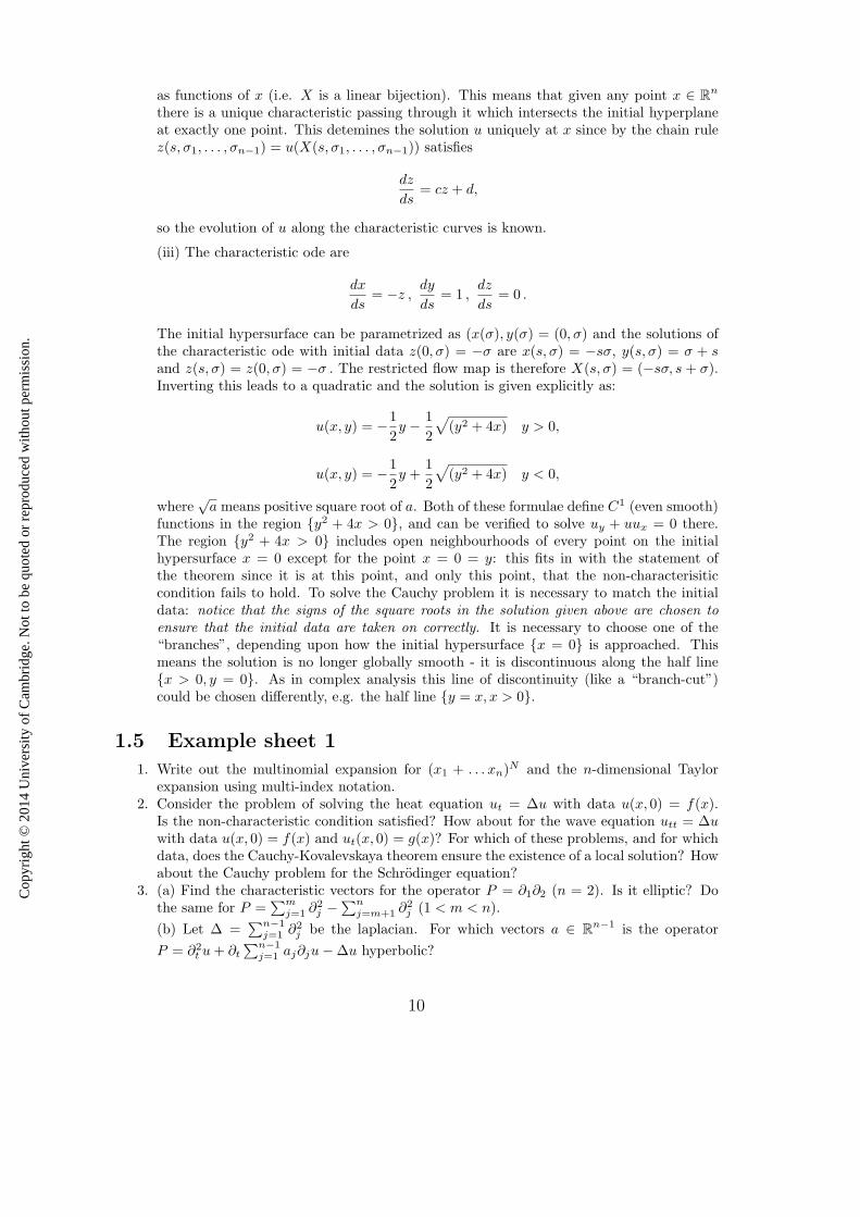
The initial hypersurface can be parametrized as (x(σ), y(σ) = (0, σ) and the solutions ofthe characteristic ode with initial data z(0, σ) = −σ are x(s, σ) = −sσ, y(s, σ) = σ + sand z(s, σ) = z(0, σ) = −σ . The restricted flow map is therefore X(s, σ) = (−sσ, s + σ).Inverting this leads to a quadratic and the solution is given explicitly as:

u(x, y) = −1

2y − 1

2

√(y2 + 4x) y > 0,

u(x, y) = −1

2y +

1

2

√(y2 + 4x) y < 0,

where√

a means positive square root of a. Both of these formulae define C1 (even smooth)functions in the region y2 + 4x > 0, and can be verified to solve uy + uux = 0 there.The region y2 + 4x > 0 includes open neighbourhoods of every point on the initialhypersurface x = 0 except for the point x = 0 = y: this fits in with the statement ofthe theorem since it is at this point, and only this point, that the non-characterisiticcondition fails to hold. To solve the Cauchy problem it is necessary to match the initialdata: notice that the signs of the square roots in the solution given above are chosen toensure that the initial data are taken on correctly. It is necessary to choose one of the“branches”, depending upon how the initial hypersurface x = 0 is approached. Thismeans the solution is no longer globally smooth - it is discontinuous along the half linex > 0, y = 0. As in complex analysis this line of discontinuity (like a “branch-cut”)could be chosen differently, e.g. the half line y = x, x > 0.

1.5 Example sheet 1

1. Write out the multinomial expansion for (x1 + . . . xn)N and the n-dimensional Taylorexpansion using multi-index notation.

2. Consider the problem of solving the heat equation ut = ∆u with data u(x, 0) = f(x).Is the non-characteristic condition satisfied? How about for the wave equation utt = ∆uwith data u(x, 0) = f(x) and ut(x, 0) = g(x)? For which of these problems, and for whichdata, does the Cauchy-Kovalevskaya theorem ensure the existence of a local solution? Howabout the Cauchy problem for the Schrodinger equation?

3. (a) Find the characteristic vectors for the operator P = ∂1∂2 (n = 2). Is it elliptic? Dothe same for P =

∑mj=1 ∂2

j − ∑nj=m+1 ∂2

j (1 < m < n).

(b) Let ∆ =∑n−1

j=1 ∂2j be the laplacian. For which vectors a ∈ R

n−1 is the operator

P = ∂2t u + ∂t

∑n−1j=1 aj∂ju − ∆u hyperbolic?

10

Cop

yrig

ht ©

201

4 U

nive

rsity

of C

ambr

idge

. Not

to b

e qu

oted

or

repr

oduc

ed w

ithou

t per

mis

sion

.

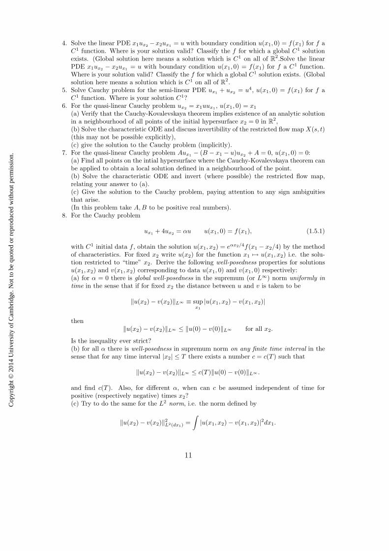
4. Solve the linear PDE x1ux2−x2ux1

= u with boundary condition u(x1, 0) = f(x1) for f aC1 function. Where is your solution valid? Classify the f for which a global C1 solutionexists. (Global solution here means a solution which is C1 on all of R

2.Solve the linearPDE x1ux2

− x2ux1= u with boundary condition u(x1, 0) = f(x1) for f a C1 function.

Where is your solution valid? Classify the f for which a global C1 solution exists. (Globalsolution here means a solution which is C1 on all of R

2.5. Solve Cauchy problem for the semi-linear PDE ux1

+ ux2= u4, u(x1, 0) = f(x1) for f a

C1 function. Where is your solution C1?6. For the quasi-linear Cauchy problem ux2

= x1uux1, u(x1, 0) = x1

(a) Verify that the Cauchy-Kovalevskaya theorem implies existence of an analytic solutionin a neighbourhood of all points of the initial hypersurface x2 = 0 in R

2,(b) Solve the characteristic ODE and discuss invertibility of the restricted flow map X(s, t)(this may not be possible explicitly),(c) give the solution to the Cauchy problem (implicitly).

7. For the quasi-linear Cauchy problem Aux1− (B − x1 − u)ux2

+ A = 0, u(x1, 0) = 0:(a) Find all points on the intial hypersurface where the Cauchy-Kovalevskaya theorem canbe applied to obtain a local solution defined in a neighbourhood of the point.(b) Solve the characteristic ODE and invert (where possible) the restricted flow map,relating your answer to (a).(c) Give the solution to the Cauchy problem, paying attention to any sign ambiguitiesthat arise.(In this problem take A,B to be positive real numbers).

8. For the Cauchy problem

ux1+ 4ux2

= αu u(x1, 0) = f(x1), (1.5.1)

with C1 initial data f , obtain the solution u(x1, x2) = eαx2/4f(x1 − x2/4) by the methodof characteristics. For fixed x2 write u(x2) for the function x1 7→ u(x1, x2) i.e. the solu-tion restricted to “time” x2. Derive the following well-posedness properties for solutionsu(x1, x2) and v(x1, x2) corresponding to data u(x1, 0) and v(x1, 0) respectively:(a) for α = 0 there is global well-posedness in the supremum (or L∞) norm uniformly intime in the sense that if for fixed x2 the distance between u and v is taken to be

‖u(x2) − v(x2)‖L∞ ≡ supx1

|u(x1, x2) − v(x1, x2)|

then‖u(x2) − v(x2)‖L∞ ≤ ‖u(0) − v(0)‖L∞ for all x2.

Is the inequality ever strict?(b) for all α there is well-posedness in supremum norm on any finite time interval in thesense that for any time interval |x2| ≤ T there exists a number c = c(T ) such that

‖u(x2) − v(x2)‖L∞ ≤ c(T )‖u(0) − v(0)‖L∞ .

and find c(T ). Also, for different α, when can c be assumed independent of time forpositive (respectively negative) times x2?(c) Try to do the same for the L2 norm, i.e. the norm defined by

‖u(x2) − v(x2)‖2L2(dx1)

=

∫|u(x1, x2) − v(x1, x2)|2dx1.

11

Cop

yrig

ht ©

201

4 U

nive

rsity

of C

ambr

idge

. Not

to b

e qu

oted

or

repr

oduc

ed w

ithou

t per

mis

sion

.

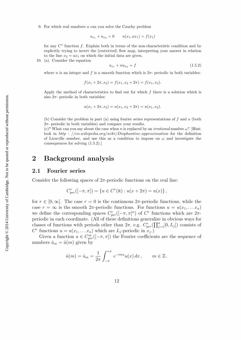
9. For which real numbers a can you solve the Cauchy problem

ux1+ ux2

= 0 u(x1, ax1) = f(x1)

for any C1 function f . Explain both in terms of the non-characteristic condition and byexplicitly trying to invert the (restricted) flow map, interpreting your answer in relationto the line x2 = ax1 on which the initial data are given.

10. (a). Consider the equationux1

+ nux2= f (1.5.2)

where n is an integer and f is a smooth function which is 2π- periodic in both variables:

f(x1 + 2π, x2) = f(x1, x2 + 2π) = f(x1, x2).

Apply the method of characteristics to find out for which f there is a solution which isalso 2π- periodic in both variables:

u(x1 + 2π, x2) = u(x1, x2 + 2π) = u(x1, x2).

(b) Consider the problem in part (a) using fourier series representations of f and u (both2π- periodic in both variables) and compare your results.(c)* What can you say about the case when n is replaced by an irrational number ω? [Hint:look in http : //en.wikipedia.org/wiki/Diophantine approximation for the definitionof Liouville number, and use this as a condition to impose on ω and investigate theconsequences for solving (1.5.2).]

2 Background analysis

2.1 Fourier series

Consider the following spaces of 2π-periodic functions on the real line:

Crper([−π, π]) = u ∈ Cr(R) : u(x + 2π) = u(x) ,

for r ∈ [0,∞]. The case r = 0 is the continuous 2π-periodic functions, while thecase r = ∞ is ths smooth 2π-periodic functions. For functions u = u(x1, . . . xn)we define the corresponding spaces Cr

per([−π, π]n) of Cr functions which are 2π-periodic in each coordinate. (All of these definitions generalize in obvious ways forclasses of functions with periods other than 2π, e.g. Cr

per(∏n

j=1[0, Lj]) consists ofCr functions u = u(x1, . . . xn) which are Lj-periodic in xj.)

Given a function u ∈ C∞per([−π, π]) the Fourier coefficients are the sequence of

numbers um = u(m) given by

u(m) = um =1

2π

∫ +π

−π

e−imxu(x) dx , m ∈ Z .

12

Cop

yrig

ht ©

201

4 U

nive

rsity

of C

ambr

idge

. Not

to b

e qu

oted

or

repr

oduc

ed w

ithou

t per

mis

sion

.

Integration by parts gives the formula ∂αu(m) = (im)αu(m) for positive integralα, which shows that the sequence of Fourier coefficients is a rapidly decreasing(bi-infinite) sequence: this means that u ∈ s(Z) where

s(Z) = u : Z → C such that |u|α = supm∈Z

|mαu(m)| < ∞ ∀α ∈ Z+ .

This in turn means that the series∑

m∈Zu(m)eimx converges absolutely and uni-

formly to a smooth function. The central fact about Fourier series is that thisseries actually converges to u, so that each u ∈ C∞

per([−π, π]) can be representedas:

u(x) =∑

u(m)eimx , where u(m) =1

2π

∫ +π

−π

e−imxu(x) dx .

The whole development works for periodic functions u = u(x1, . . . xn) with thesequence space generalized to

s(Zn) = u : Zn → C such that |u|α = supm∈Zn

|mαu(m)| < ∞ ∀α ∈ Zn+ .

Here we use multi-index notation, in terms of which we have:

Theorem 2.1.1 The mappping

C∞per([−π, π]n) → s(Zn) ,

u 7→ u = u(m)m∈Zn where u(m) =1

(2π)n

∫

[−π,π]ne−im·xu(x) dx

is a linear bijection whose inverse is the map which takes u to∑

m∈Zn u(m)eim·x

and the following hold:

1. u(x) =∑

m∈Zn u(m)eim·x where u(m) = 1(2π)n

∫[−π,π]n

e−im·xu(x) dx (Fourier

inversion),

2. ∂αu(m) = (im)αu(m) for all m ∈ Zn, α ∈ Zn+,

3. 1(2π)n

∫[−π,π]n

|u(x)|2 dx =∑

m∈Zn |u(m)|2 (Parseval-Plancherel).

2.2 Fourier transform

Define the Schwartz space of test functions:

S(Rn) = u ∈ C∞(Rn) : |u|α,β = supx∈R

n

|xα∂βu(x)| < ∞ , ∀α ∈ Zn+, β ∈ Zn

+ .

This is a convenient space on which to define the Fourier transform because of thefact that Fourier integrals interchange rapidity of decrease with smoothness, sothe space of functions which are smooth and rapidly decreasing is invariant underFourier transform:

13

Cop

yrig

ht ©

201

4 U

nive

rsity

of C

ambr

idge

. Not

to b

e qu

oted

or

repr

oduc

ed w

ithou

t per

mis

sion

.

Theorem 2.2.1 The Fourier transform, i.e. the mapping

F : S(Rn) → S(Rn) ,

u 7→ u where u(ξ) = Fx→ξ(u(x)) =

∫

Rn

e−iξ·xu(x) dx

is a linear bijection whose inverse is the map F−1 which takes v to the functionv = F−1(v) given by

v(x) =1

(2π)n

∫

Rn

e+iξ·xv(ξ) dξ ,

and the following hold:

1. u(x) = 1(2π)n

∫Rn u(ξ)eiξ·xdξ where u(ξ) =

∫Rn e−iξ·xu(x) dx (Fourier inver-

sion),

2. ∂αu(ξ) = Fx→ξ(∂αu(x)) = (iξ)αu(ξ) and (∂αu)(ξ) = Fx→ξ((−ix)αu(x)) for

all x, ξ ∈ Rn, α ∈ Zn

+,

3.∫

Rn v(ξ)u(ξ) dξ =∫

Rn v(x)u(x) dx ,

4. 1(2π)n

∫Rn v(ξ)u(ξ) dξ =

∫Rn v(x)u(x) dx (Parseval-Plancherel),

5. u ∗ v = uv where u ∗ v =∫

u(x − y)v(y) dy (convolution).

2.3 Banach spaces

A norm on a vector space X is a real function x 7→ ‖x‖ such that

1. ‖x‖ ≥ 0 with equality iff x = 0,

2. ‖cx‖ = |c|‖x‖ for all c ∈ C,

3. ‖x + y‖ ≤ ‖x‖ + ‖y‖ .

(If the first condition is replaced by the weaker requirement 1′ that ‖x‖ ≥ 0 thenthe modified conditions 1′, 2, 3 define a semi-norm.) A normed vector space is ametric space with metric d(x, y) = ‖x − y‖. Recall that a metric on X is a mapd : X × X → [0,∞) such that

1. d(x, y) ≥ 0 with equality iff x = y,

2. d(x, y) = d(y, x)

3. d(x, z) ≤ d(x, y) + d(y, z) for all x, y, z in X.

14

Cop

yrig

ht ©

201

4 U

nive

rsity

of C

ambr

idge

. Not

to b

e qu

oted

or

repr

oduc

ed w

ithou

t per

mis

sion

.

(This definition does not require that X be a vector space.) The metric space(X, d) is complete if every Cauchy sequence has a limit point: to be precise ifxj∞j=1 has the property that ∀ǫ > 0 there exists N(ǫ) ∈ N such that j, k ≥N(ǫ) =⇒ d(xj, xk) < ǫ then there exists x ∈ X such that limj→∞ d(xj, x) = 0.

Definition 2.3.1 A Banach space is a normed vector space which is complete(using the metric d(x, y) = ‖x − y‖).Examples are

• Cn with the Euclidean norm ‖z‖ = (

∑j |zj|2)

1

2 .

• C([a, b]) with ‖f‖ = sup[a,b] |f(x)| (uniform norm).

• Spaces of p-summable (bi-infinite) sequences um = u(m)m∈Z

lp(Z) = u : Z → C such that ‖u‖p = (∑

|u(m)|p) 1

p < ∞

and generalizations such as lp(Zn) and lp(N).

• Spaces of measurable Lp functions for 1 ≤ p < ∞

Lp(Rn) = u : Rn → C measurable with ‖u‖p = (

∫|u(x)‖p dx )

1

p < ∞

and generalizations such as Lp([−π, π]n) and Lp([0,∞)) etc. For p = ∞ thespace L∞(Rn) consists of measurable functions which are bounded on thecomplement of a null set, and the least such bound is called the essentialsupremum and gives the norm ‖u‖L∞ . In this example we identify functionswhich agree on the complement of a null set (almost everywhere). Read theappendix for an informal introduction to the Lebesgue spaces and a list ofresults from integration that we will use in this course1.

Completeness is important because methods for proving that an equation hasa solution typically produce a sequence of “approximate solutions”, e.g. Picarditerates for the case of ode. If this sequence can be shown to be Cauchy in somenorm then completeness ensures the existence of a limit point which is the putativesolution, and in good situations can be proved to be a solution. The basic result isthe contraction mapping principle which can be used to prove existence of solutionsof equations of the form Tx = x, i.e. to find fixed points of mappings T : X → Xdefined on complete (non-empty) metric spaces:

Theorem 2.3.2 Let (X, d) be a complete, non-empty, metric space and T : X →X a map such that

d(Ty1, T y2) ≤ kd(y1, y2)

with k ∈ (0, 1). Then T has a unique fixed point in X; in fact if y0 ∈ X, then Tmy0

converges to a fixed point as m → ∞.

1You will not be examined on any subtle points connected with the Lebesgue integral

15

Cop

yrig

ht ©

201

4 U

nive

rsity

of C

ambr

idge

. Not

to b

e qu

oted

or

repr

oduc

ed w

ithou

t per

mis

sion

.

Proof We first prove uniqueness of any fixed point: notice that if Ty1 = y1 andTy2 = y2 then the contraction property implies

d(y1, y2) = d(Ty1, T y2) ≤ kd(y1, y2)

and therefore, since 0 < k < 1, we have d(y1, y2) = 0 and so y1 = y2.To prove existence, firstly, by the triangle inequality:

d(T n+r+1y0, Tny0) ≤

r∑

m=0

d(T n+m+1y0, Tn+my0)

≤r∑

m=0

kmd(T n+1y0, Tny0) ≤

r∑

m=0

kn+md(Ty0, y0) .

But 0 < k < 1 implies that∑

m≥0 km = 11−k

< ∞ and hence Tmy0 forms aCauchy sequence in X. So by completeness of X, Tmy0 → y some y. But thenTm+1y0 → Ty, because T is continuous by the contraction property, and so Ty = yand y is a fixed point. Thus T has a unique fixed point. 2

Now review the proof of the existence theorem for ode via the contractionmapping theorem in the Banach space of continuous functions with the uniformnorm in §2.8. Theorem 2.8.4 says that for ode defined by Lipschitz vector fieldsthe solutions vary continuously with the initial data: this is the crucial propertyof well-posedness. For pde the issue is more subtle as will now be discussed.

Norms are used in the definition of well posed: if a pde can be solved for asolution u which is uniquely determined by some set of initial and/or boundarydata fj then the problem is said to be well posed in a norm ‖ · ‖ if the solutionchanges a small amount in this norm as the data change. This would be satisfiedif for example for any other solution v determined by data gj there holds:

‖u − v‖ ≤ C(∑

j

‖fj − gj‖j) , for some C > 0 , (2.3.1)

where ‖ · ‖j are some collection of norms which measure what kind of changes ofdata produce small changes of the solution. Finding the appropriate norms suchthat (2.3.1) holds for a given problem is a crucial part of understanding the problem- they are generally not known in advance. Once this is understood it is helpfulwith development of numerical methods for solving problems on computers, andtells you in an experimental situation how accurately you need to measure the datato make a good prediction.

To fix ideas consider the problem of solving an evolution equation of the form

∂tu = P (∂x)u

where P is a constant coefficient polynomial; e.g. the case P (∂x) = i∂2x corresponds

to the Schrodinger equation ∂tu = i∂2xu. If we are solving this with periodic

16

Cop

yrig

ht ©

201

4 U

nive

rsity

of C

ambr

idge

. Not

to b

e qu

oted

or

repr

oduc

ed w

ithou

t per

mis

sion

.

boundary conditions u(x, t) = u(x + 2π, t) and with given initial data u(x, 0) =u0(x) for u0 ∈ C∞

per([−π, π]). Formally the solution can be given as

u(x, t) =∑

m∈Z

etP (im)+imxu0(m) (2.3.2)

and if the initial data uo =∑

u0(m)eimx is a finite sum of exponentials then (2.3.2)is easily seen to define a solution since it reduces also to a finite sum. In the generalcase it is necessary to investigate convergence of the sum so that it does define asolution, then to prove uniqueness of this solution, and finally to find norms forwhich well-posedness holds. For this final step the Parseval identity is often veryhelpful, and for the case of the Schrodinger equation the series (2.3.2) does indeeddefine a solution for smooth periodic data u0, v0 and

maxt∈R

∫|u(x, t) − v(x, t)|2 dx ≤

∫|u0(x) − v0(x)|2 dx .

This inequality would be interpreted as saying that the Schrodinger equation iswell posed in L2 (globally in time since there is no restriction on t.) In question 7of sheet II you are asked to prove that the solutions are unique.

In general an equation defines a well posed problem with respect to specificnorms, which encode certain aspects of the behaviour of the solutions and haveto be found as part of the investigation: the property of being well posed dependson the norm. This is related to the fact that norms on infinite dimensional vectorspaces (like spaces of functions) can be inequivalent (i.e. can correspond to differentnotions of convergence), unlike in Euclidean space R

n.

2.4 Hilbert spaces

A Hilbert space is a Banach space which is also an inner product space: the norm

arises as ‖x‖ = (x, x)1

2 where (·, ·) : X × X → C satisfies:

1. (x, x) ≥ 0 with equality iff x = 0,

2. (x, y) = (y, x),

3. (ax + by, z) = a (x, z) + b (y, z) and (x, ay + bz) = a (x, y) + b (x, z) for com-plex numbers a, b and vectors x, y, z.

(Funtions X × X → C like this which are linear in the second variable and anti-linear in the first are sometimes called sesqui-linear.) Crucial properties of the innerproduct in a Hilbert space are the Cauchy-Schwarz inequality | (x, y) | ≤ ‖x‖‖y‖and the fact that the inner product can be recovered from the norm via

(x, y) =1

4

(‖x + y‖2 − ‖x − y‖2 − i‖x + iy‖2 + i‖x − iy‖2

), (polarization) .

17

Cop

yrig

ht ©

201

4 U

nive

rsity

of C

ambr

idge

. Not

to b

e qu

oted

or

repr

oduc

ed w

ithou

t per

mis

sion

.

Examples include l2(Zn) with inner product∑

m u(m)v(m) and L2(Rn) with inner

product (u, v) =∫

u(x)v(x) dx. Another example is the Sobolev spaces: firstly inthe periodic case

H1(R/2πZ) = u ∈ L2([−π, π]) : ‖u‖21 =

∑

m∈Z

(1 + |m|2)|u(m)|2 < ∞ , (2.4.1)

where u =∑

u(m)eimx is the Fourier representation, and secondly

H1(Rn) = u ∈ L2(Rn) : ‖u‖21 =

∫

Rn

(1 + |ξ|2)|u(ξ)|2 dξ < ∞ , (2.4.2)

where u is the Fourier transform.The new structure in Hilbert (as compared to Banach) spaces is the notion of

orthogonality coming from the the inner product. A set of vectors en is calledorthonormal if (en, em) = δnm. We will consider only Hilbert spaces which have acountable orthonormal basis en (separable Hilbert spaces). In such spaces it ispossible to decompose arbitrary elements as u =

∑unen where un = (en, u). (The

case of Fourier series with em(x) = eimx/√

2π,m ∈ Z is an example.) The Parsevalidentity in abstract form reads ‖u‖2 =

∑ | (en, u) |2 and:

Theorem 2.4.1 Given an orthonormal set en the following are equivalent:

• (en, u) = 0 ∀n implies u = 0, (completeness)

• ‖u‖2 =∑ | (en, u) |2 ∀u ∈ X, (Parseval),

• u =∑

(en, u) en ∀u ∈ X (orthonormal basis).

A closed subspace X1 ⊂ X of a Hilbert space is also a Hilbert space, and thereis an orthogonal decomposition

X = X1 ⊕ X⊥1

where X⊥1 = y ∈ X : (x1, y) = 0∀x1 ∈ X1. This means that any x ∈ X can

be written uniquely as x = x1 + y with x1 ∈ X1 and y ∈ X⊥1 , and there is a

correponding projection PX1x = x1.

Associated to a Hilbert space X is its dual space X ′ which is defined to be thespace a bounded linear maps:

X ′ = L : X → C , with L linear and ‖L‖ = supx∈X,‖x‖=1

|Lx| < ∞.

The definition of the norm on X ′ ensures that |L(x)| ≤ ‖L‖‖x‖.Theorem 2.4.2 (Riesz representation) Given a bounded linear map L on aHilbert space X there exists a unique vector y ∈ X such that Lx = (y, x); also‖L‖ = ‖y‖. The correspondence between L and y gives an identification of thedual space X ′ with the original Hilbert space X.

18

Cop

yrig

ht ©

201

4 U

nive

rsity

of C

ambr

idge

. Not

to b

e qu

oted

or

repr

oduc

ed w

ithou

t per

mis

sion

.

A generalization of this (for non-symmetric situations) is:

Theorem 2.4.3 (Lax-Milgram lemma) Given a bounded linear map L : X →R on a Hilbert space X, and a bilinear map B : X × X → R which satisfies (forsome positive numbers ‖B‖, γ):

• |B(x, y)| ≤ ‖B‖‖x‖‖y‖ ∀x, y ∈ X (continuity),

• B(x, x) ≥ γ‖x‖2 ∀x ∈ X (coercivity),

there exists a unique vector y ∈ X such that Lx = B(y, x)∀x ∈ X.

A bounded linear operator B : X → X means a linear map X → X with theproperty that there exists a number ‖B‖ ≥ 0 such that ‖Bu‖ ≤ ‖B‖‖u‖ ∀u ∈ X.As in Sturm-Liouville theory we say a bounded linear operator is diagonalizableif there is an orthonormal basis en such that Ben = λnen for some collection ofcomplex numbers λn which are the eigenvalues.

2.5 Distributions

Definition 2.5.1 A periodic distribution T ∈ C∞per([−π, π]n)′ is a continuous lin-

ear map T : C∞per([−π, π]n) → C, where continuous means that if fn and all its

partial derivatives ∂αfn converge uniformly to f then T (fn) → T (f). Here we callC∞

per([−π, π]n) the space of test functions.A tempered distribution T ∈ S ′(Rn) is a continuous linear map T : S(Rn) → C,

where continuous means that if ‖fn − f‖α,β → 0 for every Schwartz semi-normthen T (fn) → T (f). Here we call S(Rn) the space of test functions.

In both cases for x0 ∈ Rn any fixed point (which may be taken to lie in [−π, π]n

in the periodic case) the Dirac distribution defined by δx0(f) = f(x0) gives an

example.

Remark 2.5.2 The notion of convergence on C∞per([−π, π]n and S(Rn) used in

this definition makes these spaces into topological spaces in which the convergencemust be with respect to a countable family of semi-norms. These are examplesof Frechet spaces, a class of topological vector spaces which generalize the notionof Banach space by using a countable family of semi-norms rather than a singlenorm to define a notion of convergence. Using this notion of convergence one cancheck that the Fourier transform F is continuous as is its inverse, and the Fourierinversion theorem can be summarized by the assertion that F : S(Rn) → S(Rn) isa linear homeomorphism with inverse F−1.

Remark 2.5.3 Notice that integrable functions define distributions in a naturalway: in the simplest case if g is continuous 2π-periodic function then the formulaTg(f) =

∫[−π,π]

g(x)f(x) dx defines a periodic distribution and clearly the mapping

19

Cop

yrig

ht ©

201

4 U

nive

rsity

of C

ambr

idge

. Not

to b

e qu

oted

or

repr

oduc

ed w

ithou

t per

mis

sion

.

g 7→ Tg is an injection of Cper([−π, π]) into (C∞per([−π, π]))′. Similarly if g is

absolutely integrable on Rn then the formula Tg(f) =

∫Rn g(x)f(x) dx defines a

tempered distribution. The mapping g 7→ Tg is, properly interpreted, injective: ifg ∈ L1(Rn) then Tg(f) = 0 for all f ∈ S(Rn) implies that g = 0 almost everywhere.On account of this remark distributions are often called “generalized functions”.The Dirac example indicates that there are distrubutions which do not arise as Tg.

Remark 2.5.4 In these definitions distributions are elements of the dual spaceof a space of test functions with a specified notion of convergence ( a topology).Another frequently used class of distributions is the dual space of C∞

0 (Rn) the spaceof compactly supported smooth functions, topologized as follows: fn → f in C∞

0

if there is a fixed compact set K such that all fn, f are supported in K and if allpartial derivatives of ∂αfn converge (uniformly) to ∂αf . This class of distributionsis more convenient for some purposes, but not for using the Fourier transform, forwhich purpose the tempered distributions are most convenient because of remark2.5.2, which allows the fourier transform to be defined on tempered distributions“by duality” as we now discuss.

Operations are defined on distributions by using duality to transfer them to thetest functions, e.g.:

• Given T ∈ S ′(Rn) an arbitrary partial derivative ∂αT is defined by ∂αT (f) =(−1)|α|T (∂αf).

• Given T ∈ S ′(Rn) its fourier transform T is defined by T (f) = T (f).

• Given T ∈ S ′(Rn) and χ ∈ S(Rn) the distribution χT is defined by χT (f) =T (χf). This is also the definition if χ is a polynomial - it makes sense becausea polynomial times a Schwartz function is again a Schwartz function.

It is useful to check, with reference to the fact in remark 2.5.3 that distributionsare generalized functions, that all such defintions of operations on distributions aredesigned to extend the corresponding definitions on functions: e.g. for a Schwartzfunction g we have

∂αTg = T∂αg ,

where on the left ∂α means distributional derivative while on the right it is theusual derivative from calculus applied to the test function g. The same principleis behind the other definitions.

There are various alternate notations used for distributions:

T (f) = 〈T , f〉 =

∫T (x)f(x) dx

where in the right hand version it should be remembered that the expression ispurely formal in general: the putative function T (x) has not been defined, and

20

Cop

yrig

ht ©

201

4 U

nive

rsity

of C

ambr

idge

. Not

to b

e qu

oted

or

repr

oduc

ed w

ithou

t per

mis

sion

.

the integral notation is not an integral - just shorthand for the duality pairing ofthe definition. It is nevertheless helpful to use it to remember some formulae: forexample the formula for the distributional derivative takes the form

∂αT (f) =

∫∂αT (x)f(x) dx = (−1)|α|

∫T (x)∂αf(x) dx = (−1)|α|T (∂αf) ,

which is “familiar” from integration by parts. The formula∫

δ(x − x0)f(x) dx =f(x0) and related ones are to be understood as formal expressions for the properdefinition of the delta distribution above.

2.6 Positive distributions and Measures

In this section2 we restrict to 2π-periodic distributions on the real line for simplic-ity. The delta distribution δx0

has the property that if f ≥ 0 then δx0(f) ≥ 0;

such distributions are called positive. Positive distributions have an importantcontinuity property as a result: if T is any positive periodic distribution, thensince

−‖f‖L∞ ≤ f(x) ≤ ‖f‖L∞ , ‖f‖ = sup |f(x)|for each f ∈ C∞

per([−π, π]) it follows from positivity that T (‖f‖L∞ ± f) ≥ 0 andhence by linearity that

−c‖f‖L∞ ≤ T (f) ≤ c‖f‖L∞

where c = T (1) is a positive number. This inequality, applied with f replacedby f − fn, means that if fn → f uniformly then T (fn) → T (f), i.e. positivedistributions are automatically continuous with respect to uniform convergence,in strong contrast to the continuity property required in the original definition.In fact this new continuity property ensures that a positive distribution can beextended uniquely as a map

L : Cper([−π, π]) → R

i.e. as a continuous linear functional on the space of continuous functions. Thisextension is an immediate consquence of the density of smooth functions in thecontinuous functions in the uniform norm (which can be deduced from the Weier-strass approximation theorem). A much more lengthy argument allows such afunctional to be extended as an integral L(f) =

∫f dµ which is defined for a class

of measurable functions f which contains and is bigger than the class of continu-ous functions. To conclude: positive distributions automatically extend to definecontinuous linear functional on the space of continuous functions, and hence canbe identified with a class of measures (Radon measures) which can be used to inte-grate much larger classes of functions (extending further the domain of the originaldistribution).

2This is an optional section, for background only

21

Cop

yrig

ht ©

201

4 U

nive

rsity

of C

ambr

idge

. Not

to b

e qu

oted

or

repr

oduc

ed w

ithou

t per

mis

sion

.

2.7 Sobolev spaces

We define the Sobolev spaces for s = 0, 1, 2, . . . on various domains:

On Rn: we have the following equivalent definitions:

Hs(Rn) = u ∈ L2(Rn) : ‖u‖2Hs =

∑

α:|α|≤s

‖∂αu‖2L2 < ∞

= u ∈ L2(Rn) :

∫

Rn

(1 + ‖ξ‖2)s|u(ξ)|2 dξ < ∞

= C∞0 (Rn)

‖·‖Hs

.

In the first line the partial derivatives are taken in the distributional sense: theprecise meaning is that all distributional (=weak) partial derivatives up to orders of the distribution Tu determined by u are distributions which are determinedby square integrable funtions which are designated ∂αu (i.e. ∂αTu = T∂αu with∂αu ∈ L2 in the notation introduced previously). The final line means that Hs isthe closure of the space of smooth compactly supported functions C∞

0 (Rn) in the

Sobolev norm ‖ · ‖Hs . The quantity ‖u‖2Hs =

∫Rn (1 + ‖ξ‖2)s|u(ξ)|2 dξ appearing

in the middle definition defines a norm which is equivalent to the norm ‖u‖Hs

appearing in the first definition. (Recall that ‖ · ‖ and ‖ · ‖ are equivalent if there

exist positive numbers C1, C2 such that ‖u‖ ≤ C1‖u‖ and ‖u‖ ≤ C2‖u‖ for allvectors u; equivalent norms give rise to identical notions of convergence (i.e. theydefine the same topologies).

Theorem 2.7.1 For s = 0, 1, 2 . . . the Sobolev space Hs(Rn) is a Hilbert space,and so complete in either of the norms

‖u‖2Hs =

∑

α:|α|≤s

‖∂αu‖2L2 or ‖u‖2

Hs =

∫

Rn

(1 + ‖ξ‖2)s|u(ξ)|2 dξ

which are equivalent. Given any u ∈ Hs(Rn) there exists a sequence uν of C∞0 (Rn)

functions such that ‖u − uν‖Hs → 0 as ν → +∞ . If u ∈ Hs(Rn) for s > n2

+ kwith k ∈ Z+ then u ∈ Ck(Rn) and there exists C > 0 such that

‖u‖Ck =∑

|α|≤k

supx∈Rn

|∂αu(x)| ≤ C‖u‖Hs . (2.7.1)

• The fact that Hs functions can be approximated by C∞0 (Rn) functions means

that for many purposes calculations can be done with C∞0 (Rn), or S(Rn),

functions and in the end the result extended to Hs. See the second workedproblem to see how this goes to prove (2.7.1) with k = 0.

• For s = 0 we have H0 = L2 and the norm ‖ · ‖H0 is exactly the L2 norm,

while ‖ · ‖H0 is proportional (and hence equivalent) to the L2 norm by theParseval-Plancherel theorem.

22

Cop

yrig

ht ©

201

4 U

nive

rsity

of C

ambr

idge

. Not

to b

e qu

oted

or

repr

oduc

ed w

ithou

t per

mis

sion

.

• Strictly speaking the assertion u ∈ Ck(Rn) in the last sentence of the theoremonly holds after possibly redefining u on a set of zero measure. This subtlepoint, which will generally be ignored in the following, arises because u isreally only a distribution which can be represented by an L2 function, andas such is only defined up to sets of zero measure.

On (R/(2πZ))n : In the 2π-periodic case the following definitions are equivalent:

Hsper([−π, π]n) = u ∈ L2([−π, π]n) : ‖u‖2

Hs =∑

α:|α|≤s

‖∂αu‖2L2 < ∞

= ∑

m∈Zn

u(m)eim·x :∑

m∈Zn

(1 + ‖m‖2)s|u(m)|2 < ∞

= C∞per([−π, π]n)

‖·‖Hs

.

Again the quantity apearing in the middle line defines an equivalent norm whichcan be used when it is more convenient. Since we are considering only the case s =0, 1, 2, . . . the Fourier series

∑m∈Zn u(m)eim·x always defines a square integrable

function, and as s increases the function so defined is more and more regular(exercise), and as above we have:

Theorem 2.7.2 For s = 0, 1, 2 . . . the periodic Sobolev space Hsper([−π, π]n) is a

Hilbert space, and so complete in either of the norms

‖u‖2Hs =

∑

α:|α|≤s

‖∂αu‖2L2 or ‖u‖2

Hs =∑

m∈Zn

(1 + ‖m‖2)s|u(m)|2

which are equivalent. Given any u ∈ Hsper([−π, π]n) there exists a sequence uν of

C∞per([−π, π]n) functions such that ‖u−uν‖Hs → 0 as ν → +∞ . If u ∈ Hs([−π, π]n)

for s > n2

+ k with k ∈ Z+ then u ∈ Ck(Rn) and there exists C > 0 such that

‖u‖Ck =∑

|α|≤k

supx∈[−π,π]n

|∂αu(x)| ≤ C‖u‖Hs . (2.7.2)

Similar comments to those made after Theorem 2.7.1 apply of course. To keep thenotation clean we do not indicate “periodic” in the notation for norm on a spaceof periodic functions, only the space - it should be clear from the context.

These definitions require some modifications for the case of general domainsΩ, starting with the notion of the weak partial derivative (since we did not definedistributions in Ω).

Definition 2.7.3 A locally integrable function u defined on an open set Ω admitsa weak partial derivative corresponding to the multi-index α if there exists a locallyintegrable function, designated ∂αu, with the property that∫

Ω

u ∂αχdx = (−1)|α|∫

Ω

∂αuχ dx ,

for every χ ∈ C∞0 (Ω).

23

Cop

yrig

ht ©

201

4 U

nive

rsity

of C

ambr

idge

. Not

to b

e qu

oted

or

repr

oduc

ed w

ithou

t per

mis

sion

.

A useful fact is that in this situation:

‖∂αu‖L2 = sup∫

Ω

u ∂αχdx : χ ∈ C∞0 (Ω) and ‖χ‖L2 = 1 . (2.7.3)

Then employing this notion of partial derivative we define (for s = 0, 1, 2, . . . ):

Hs(Ω) = u ∈ L2(Ω) : ‖u‖2Hs =

∑

α:|α|≤s

‖∂αu‖2L2 < ∞

(with all L2 norms being defined by integration over Ω). This space is to bedistinguished from the corresponding closure of the space of smooth functionssupported in a compact subset of Ω:

Hs0(Ω) = C∞

0 (Ω)‖·‖Hs

.

Since these functions are limits of functions which vanish in a neighbourhood of Ωthey are to be thought of as vanishing in some generalized sense on ∂Ω (at least inthe case s = 1, 2, . . . and if Ω has a smooth boundary ∂Ω.) The case s = 1 givesthe space H1

0 (Ω) which is the natural Hilbert space to use in order to give a weakformulation of the Dirichlet problem for the elliptic equation Pu = f on Ω.

In one dimension, with Ω = (a, b) ⊂ R the relation between H1((a, b)) andH1

0 ((a, b)) can be stated simply because all f ∈ H1((a, b)) are uniformly continuous(similar to the argument in the last part of the 2nd worked problem) and

H10 ((a, b)) = f ∈ H1((a, b)) : f(a) = f(b) = 0 .

More details and proofs can be found in the relevant chapter of the book of Brezis.In this course we need to be able to use Sobolev spaces to study pde, and we willsee that the Hs spaces are easy to work with for various reasons:

1. The “energy” methods often give rise to information about∫

u2dx or∫‖∇u‖2dx

where u is a solution of a pde, and this translates into information about thesolution in Sobolev norms. As a specific example: conservation of energy

1

2

∫(u2

t + ‖∇u‖2) dx = E = constant ,

when u is a solution of the wave equation .

2. The Parseval-Plancherel theorem means that information on Sobolev normsis often easily obtainable when the solution is written down using Fouriermethods.

3. The Sobolev spaces Hs are Hilbert spaces (complete) whose elements can beapproximated by smooth functions: in practice, this means one has the dualadvantages of smoothness of the functions and completeness of the space offunctions.

24

Cop

yrig

ht ©

201

4 U

nive

rsity

of C

ambr

idge

. Not

to b

e qu

oted

or

repr

oduc

ed w

ithou

t per

mis

sion

.

Thus typically we will do some computations for smooth solutions of pde whichgive information about their Sobolev norms, and then using density we will ex-tend the information to more general (weak) solutions lying in the Sobolev spacesthemselves. The use of the full Sobolev space is crucial in any argument relyingon completeness, typically in proving existence of a solution e.g. by variationalmethods or by the Lax-Milgram lemma.

2.8 Existence theorem for ordinary differential equations(ode)

We first note the following result:

Theorem 2.8.1 (Corollary to the contraction mapping principle) Let (X, d)be a complete, non-empty, metric space and suppose T : X → X is such that T n

is a contraction for some n ∈ N. Then T has a unique fixed point in X; in fact ify0 ∈ X, then Tmy0 converges to a fixed point as m → ∞.

Proof By Theorem 2.3.2, T n has a unique fixed point, y. We also have that

T n(Ty) = T n+1y = T (T ny) = Ty.

So Ty is also a fixed point of T n and fixed points are unique so Ty = y. AlsoTmny0 → y implies that Tmn+1y0 → Ty = y and so on, until Tmn+(n−1)y0 → y as(m → ∞). All together this implies that Tmy0 → y. 2

Theorem 2.8.2 (Existence theorem for ode) Let f(t, x) be a vector-valued con-tinuous function defined on the region

(t, x) : |t − t0| ≤ a, ‖x − x0‖ ≤ b ⊂ R × Rn

which also satisfies a Lipschitz condition in x:

‖f(t, x1) − f(t, x2)‖ ≤ L‖x1 − x2‖.

Define M = sup |f(t, x)| and h = min(a, bM

). Then the differential equation

dx

dt= f(t, x), x(t0) = x0 (2.8.1)

has a unique solution for |t − t0| ≤ h.

Proof This is a consequence of the contraction mapping theorem applied in thecomplete metric space:

X = x ∈ C([t0 − h, t0 + h], Rn) : ‖x(t) − x0‖ ≤ Mh ∀t ∈ [t0 − h, t0 + h] ,

25

Cop

yrig

ht ©

201

4 U

nive

rsity

of C

ambr

idge

. Not

to b

e qu

oted

or

repr

oduc

ed w

ithou

t per

mis

sion

.

endowed with the metric d(x1, x2) = sup|t−t0|≤h

‖x1(t)−x2(t)‖ . (Recall that a limit in

the uniform norm of continuous functions is itself continuous.)Introduce the integral operator T by the formula

(Tx)(t) = x0 +

∫ t

t0

f(s, x(s))ds. (2.8.2)

The condition Mh ≤ b implies that T : X → X. Notice that x ∈ X solves (2.8.1)if and only if Tx = x, by the fundamental theorem of calculus. In particular,observe that Tx = x implies that x ∈ X is in fact continuously differentiable.

We now assert that, for |t − t0| ≤ h,

‖T kx1(t) − T kx2(t)‖ ≤ Lk

k!|t − t0|kd(x1, x2).

For k = 0, this is obvious, and in general it follows by induction since

‖T kx1(t) − T kx2(t)‖ ≤∫ t

t0‖f(s, T k−1x1(s)) − f(s, T k−1x2(s))‖ds

≤ L∫ t

t0‖T k−1x1(s) − T k−1x2(s)‖ds

≤ Lk

(k−1)!

∫ t

t0|s − t0|k−1 ds d(x1, x2)

≤ Lk

k!|t − t0|kd(x1, x2).

This implies that T k is a contraction mapping for sufficiently large k, and so theresult follows from Theorem 2.8.1. 2

Theorem 2.8.3 (Gronwall Lemma) Let u ∈ C([t0, t1]) satisfy

u(t) ≤ A + B

∫ t

t0

u(s)ds

for t0 ≤ t ≤ t1 and some positive constants A,B . Then

u(t) ≤ AeB(t−t0) , for t0 ≤ t ≤ t1 .

Proof Define F (t) = A + B∫ t

t0u(s)ds - by the fundamental theorem of calculus

this is a C1 function which verifies F = Bu ≤ BF . It follows that e−BtF (t) isnon-increasing, so that e−BtF (t) ≤ e−Bt0F (t0) , and hence

u(t) ≤ F (t) ≤ F (t0)eB(t−t0) = AeB(t−t0)

for t0 ≤ t ≤ t1. 2

Theorem 2.8.4 (Well-posedness for ode) In the situation of Theorem 2.8.2,let y(t), w(t) be two solutions of (2.8.1) defined for t0 ≤ t ≤ t1 ≤ t0 + a and suchthat ‖y(t) − x0‖ ≤ b and ‖w(t) − x0‖ ≤ b on [t0, t1] . Then

‖y(t) − w(t)‖ ≤ ‖y(t0) − w(t0)‖eL(t−t0)

for t0 ≤ t ≤ t1 .

26

Cop

yrig

ht ©

201

4 U

nive

rsity

of C

ambr

idge

. Not

to b

e qu

oted

or

repr

oduc

ed w

ithou

t per

mis

sion

.

Proof u(t) = y(t) − w(t) satisfies, by the Lipschitz property:

‖u(t)‖ = ‖y(t) − w(t)‖ = ‖y(t0) − w(t0) +

∫ t

t0

(f(s, y(s)) − f(s, w(s))

)ds ‖

≤ ‖u(t0)‖ + L

∫ t

t0

‖u(s)‖ds .

The result is now an immediate consequence of Gronwall’s inequality. 2

2.9 Appendix: integration

The aim of this appendix3 is to give a brief review of facts from integration needed- completeness of the Lp spaces, dominated convergence and other basic theorems.We first consider the case of functions on the unit interval [0, 1]. A main achieve-ment of the Lebesgue integral is to construct complete vector spaces of functionswhere the completeness is with respect to a norm defined by an integral such asthe L2 norm ‖ · ‖L2 defined by

‖f‖2L2 =

∫ 1

0

|f(x)|2 dx .

This is a perfectly good norm on the space of continuous functions C([0, 1]), butthe resulting normed vector space is not complete (and so not a Banach space)and is not so useful as a setting for analysis. The Lebesgue framework providesa larger class of functions which can be potentially integrated - the measurablefunctions. The complete Lebesgue space L2 which this construction leads to thenconsists of (equivalence classes of) measurable functions f with ‖f‖2

L2 < ∞; hereit is necessary to consider equivalence classes of functions because functions whichare non-zero only on sets which are very small (in a certain precise sense) areinvisible to the integral, and so have to be factored out of the discussion. The“very small” sets in question are called null sets and are now defined.

2.9.1 Null sets and measurable functions on [0, 1]

An interval in [0, 1] is a subset of the form (a, b) or [a, b] or (a, b] or [a, b) (respec-tively open,closed, half open). In all cases the length of the interval is |I| = b− a.A collection of intervals Iα covers a subset A if A ⊂ ∪αIα.

Definition 2.9.1 (Null sets) For a set A ⊂ [0, 1] we define the outer measureto be

|A|∗ = infIn∞n=1

∈C

∑

n

|In| : A ⊂ ∪In

,

3This section gives a brief introduction to the results on Lebesgue integral which we make useof. You should be able to use the results listed here but will not be examined on the proofs oron any subtleties connected with the results.

27

Cop

yrig

ht ©

201

4 U

nive

rsity

of C

ambr

idge

. Not

to b

e qu

oted

or

repr

oduc

ed w

ithou

t per

mis

sion

.

where C consists of countable families of intervals in [0, 1]. A set N ⊂ [0, 1] isnull if |I|∗ = 0, i.e. if for all ǫ > 0 there exists In∞n=1 ∈ C which covers A with∑

|In| < ǫ.

Definition 2.9.2 We say f = g almost everywhere (a.e.) if f(x) = g(x) for allx /∈ N for some null set N . We say a sequence of functions fn converges to f a.e.if fn(x) → f(x) for all x /∈ N for some null set N .

Equality a.e. defines an equivalence relation, and two equivalent functions f, g aresaid to be Lebesgue or measure theoretically equivalent. One way to think aboutmeasurable functions is provided by the Lusin theorem, which says a measurablefunction is one which is “almost continuous” in the sense that it agrees with acontinuous function on the complement of a set of arbitrarily small outer measure:

Definition 2.9.3 (Measurable functions) A function f : [0, 1] → R is measur-able if for every ǫ > 0 there exists a continuous function f ǫ : [0, 1] → R and a setF ǫ such that |F ǫ|∗ < ǫ and f(x) = f ǫ(x) for all x /∈ F ǫ. We write L([0, 1]) for thespace of all measurable functions so defined.

Theorem 2.9.4 L([0, 1]) is a linear space closed under almost everywhere conver-gence: given a sequence fn ∈ L([0, 1]) of measurable functions which converges toa function f a.e. it follows that f ∈ L([0, 1]).

Definition 2.9.3 is not the usual definition of measurability - which involves thenotion of a distinguished collection of sets, the σ-algebra of measurable sets - butis equivalent to it by what is called the Lusin theorem (see for example §2.4 and§7.2 in the book Real Analysis by Folland). The Lusin theorem gives a helpful wayof thinking about measurability (the Littlewood 3 principles - see §3.3 in the bookReal Analysis by Royden and Fitzpatrick). A companion to the Lusin theorem isthe Egoroff theorem which states that given a sequence fn ∈ L([0, 1]) of measurablefunctions which converges to a function f a.e. then for every ǫ > 0 it is possible tofind a set E ⊂ [0, 1] with |E|∗ < ǫ such that fn → f uniformly on Ec = [0, 1] − E.Thus two of Littlewood’s principles say that “ a measurable function is one whichagrees with a continuous function except on a set which may be taken to havearbitrarily small size” and “a sequence of measurable functions which convergesalmost everywhere converges uniformly on the complement of a set which may beassumed to be arbitrarily small”.

2.9.2 Definition of Lp([0, 1])

An integral∫ 1

0f(x)dx can be defined of any non-negative measurable function, al-

though the value can be +∞ . When the function is continuous, or indeed Riemannintegrable, this integral agrees with the Riemann integral, and it has the followingproperties (for arbitrary non-negative measurable functions f, g):

28

Cop

yrig

ht ©

201

4 U

nive

rsity

of C

ambr

idge

. Not

to b

e qu

oted

or

repr

oduc

ed w

ithou

t per

mis

sion

.

1.∫ 1

0cf(x)dx = c

∫ 1

0f(x)dx if c > 0 ,

2.∫ 1

0(f(x) + g(x)) dx =

∫ 1

0(f(x) + g(x)) dx ,

3.∫ 1

0f(x) dx ≤

∫ 1

0g(x) dx if f ≤ g a.e.

Exercise For non-negative measurable functions f, g, show that if f = g a.e. then∫ 1

0f(x)dx =

∫ 1

0g(x)dx .

Accepting that such a definition exists, we can now define the Lp([0, 1]) spaces,which are Banach spaces of functions on which there exists a well-defined notionof the integral (called the Lebesgue integral).

Definition 2.9.5 For 1 ≤ p < ∞ define Lp([0, 1]) to be the linear space of mea-surable functions on [0, 1] with the property that

‖f‖pLp =

∫ 1

0

|f(x)|p dx < ∞ .

For the case p = ∞: firstly, say that f is essentially bounded above with upper(essential) bound M if f(x) ≤ M for x /∈ N for some null set N . Then let ess sup fbe the infimum of all upper essential bounds. Then:

Definition 2.9.6 L∞([0, 1]) is the linear space of measurable functions on [0, 1]with the property that

‖f‖L∞ = ess sup |f | < ∞ .

A crucial fact for us is that considering the spaces of equivalence classes offunctions which agree almost everywhere we obtain Banach spaces, also writtenLp([0, 1]): these “Lebesgue spaces” are vector spaces of (equivalence classes of)functions which are complete with respect to the norm ‖ · ‖Lp . (The fact that,strictly speaking, the elements of these spaces are equivalence classes of functionswhich agree almost everywhere, is often taken as understood and not repeatedlymentioned each time the spaces are made use of.)

The spaces Lp([0, 1]) contain the continuous functions, and the Lebesgue in-tegral, which is defined on the whole of these spaces, is equal to the Riemannintegral when restricted to Riemann integrable functions. These Lp([0, 1]) spacesare special cases of Lp(M) spaces which arise from abstract measure spaces M onwhich a measure µ (and a σ-algebra of measurable sets) is given; µ measures the“size” of elements of this collection of measurable sets. In the general setting theintegral of a function is often defined in terms of the measure of sets on which thefunction takes given values: for example, one development of the integral takes asstarting point the following definition for the integral of a non-negative measurablefunction: ∫

f dµ =

∫ ∞

0

µ(f > λ) dλ . (2.9.1)

29

Cop

yrig

ht ©

201

4 U

nive

rsity

of C

ambr

idge

. Not

to b

e qu

oted

or

repr

oduc

ed w

ithou

t per

mis

sion

.

The point here is that as λ increases, the sets f > λ decrease and their measureµ(f > λ) decreases also, so that (2.9.1) is well-defined as the Riemann integralof a monotone function. See the book Analysis by Lieb and Loss for a developmentalong these lines.

Other examples of measure spaces used in this course are

• Lp([a, b]) with norm (∫ b

a|f(x)|p dx)

1

p ,

• Lp([−π, π]n) with norm (∫

[−π,π]n|u(x)|p dx)

1

p , and

• Lp(Ω) with norm (∫Ω|f(x)|p dx)

1

p , where Ω ⊂ Rn is open; the case Ω = R

n

will occur most often.

2.9.3 Assorted theorems on integration

Theorem 2.9.7 (Holder inequality)∫

fgdx ≤ ‖f‖Lp‖g‖Lq for any pair of func-tions f ∈ Lp, g ∈ Lq (on any measure space) with p−1 + q−1 = 1 and p, q ∈ [1,∞].

Corollary 2.9.8 (Young inequality) If f ∈ Lp(Rn) and g ∈ L1(Rn) then f ∗g ∈Lp(Rn) and ‖f ∗ g‖Lp ≤ ‖f‖Lp‖g‖L1 for 1 ≤ p ≤ ∞.

Theorem 2.9.9 (Dominated convergence theorem) Let the sequence fn ∈L1 converge to f almost everywhere (on any measure space) and assume that thereexists a nonnegative measurable function Φ ≥ 0 such that |fn(x)| ≤ Φ(x) almosteverywhere and

∫Φ < ∞. Then limn→∞

∫fn =

∫f and limn→∞ ‖fn − f‖L1 = 0 .

Corollary 2.9.10 (Differentiation through the integral) Let g ∈ C1(Rn×Ω)where Ω ⊂ R

m is open, and consider F (λ) =∫

Rn g(x, λ)dx. Assume there exists ameasurable function Φ(x) ≥ 0 such that

•∫

Rn Φ(x) dx < ∞ ,

• supλ(|g(x, λ) + |∂λg(x, λ)|) ≤ Φ(x) .

Then F ∈ C1(Ω) and ∂λF =∫

Rn ∂λg(x, λ) dx.

Corollary 2.9.11 If f is a Ck(Rn) function with all partial derivatives ∂αf oforder |α| ≤ k bounded, and g ∈ L1(Rn) then f∗g ∈ Ck(Rn) and ∂α(f∗g) = (∂αf)∗gfor |α| ≤ k.

Theorem 2.9.12 (Tonelli) If f ≥ 0 is a nonnegative measurable function f :R

l × Rm → R then∫∫

Rl×Rm

f(x, y) dxdy =

∫

Rl

( ∫

Rm

f(x, y) dy

)dx =

∫

Rm

( ∫

Rl

f(x, y) dx

)dy .

30

Cop

yrig

ht ©

201

4 U

nive

rsity

of C

ambr

idge

. Not

to b

e qu

oted

or

repr

oduc

ed w

ithou

t per

mis

sion

.

Theorem 2.9.13 (Fubini) If f is a measurable function f : Rl × R

m → R suchthat ∫∫

Rl×Rm

|f(x, y)| dxdy < ∞

then∫∫

Rl×Rm

f(x, y) dxdy =

∫

Rl

( ∫

Rm

f(x, y) dy

)dx =

∫

Rm

( ∫

Rl

f(x, y) dx

)dy .

Remark 2.9.14 In these two results it is to be understood that when we write downrepeated integrals that an implicit assertion is that the functions y 7→

∫f(x, y)dx

and x 7→∫

f(x, y)dy are measurable and integrable.

Theorem 2.9.15 (Minkowski inequality) If f is a measurable function f :R

l × Rm → R and g : R

m → R is measurable, then

‖∫

Rm

f(x, y)g(y) dy‖Lp(dx) ≤∫

Rm

‖f(x, y)‖Lp(dx)|g(y)| dy . (2.9.2)

where

‖f(x, y)‖p

Lp(dx) =

∫

Rl

|f(x, y)|p dx ,

with the understanding as above that this means that if the right hand side of(2.9.2) is finite then the function f(x, y)g(y) is integrable in y for almost every xand the resulting function x 7→

∫f(x, y)g(y) dy is measurable and (2.9.2) holds.

2.10 Worked problems

1. Prove that if a continuous 2π-periodic function f ∈ Cper([−π, π]) satisfies

f(m) = (2π)−1

∫ +π

−π

e−imxf(x)dx = 0

for all m ∈ Z , then f is identically zero. Deduce that if f ∈ C∞per([−π, π]) then f =∑

m∈Zf(m)eimx.

Answer Assume for the sake of contradiction that there exists x0 with f(x0) 6= 0. Replacingf(·) by ±f(· − x0) we may assume w.l.o.g. that f(0) > 0. Now:

∫ +π

−π

f(x)(ǫ + cos x)k dx = 0

for all k ∈ Z+ and ǫ ∈ R, by the assumption that all Fourier coefficients vanish. Bycontinuity of f there exists δ ∈ (0, π/2] such that f(x) > f(0)/2 > 0 for |x| < δ. Nowmaxδ≤|x|≤π cos x < 1 and cos 0 = 1, so there exists

31

Cop

yrig

ht ©

201

4 U

nive

rsity

of C

ambr

idge

. Not

to b

e qu

oted

or

repr

oduc

ed w

ithou

t per

mis

sion

.

• ǫ > 0 such that |ǫ + cos x| < 1 − ǫ/2 for δ ≤ |x| ≤ π;

• η ∈ (0, δ) such that |ǫ + cos x| > 1 + ǫ/2 for |x| < η.

Now

∫ +π

−π

f(x)(ǫ + cos x)k dx =

∫

|x|≤η

+

∫

|η|<|x|<δ

+

∫

δ≤|x|≤π

f(x)(ǫ + cos x)k dx

≥ (1 +ǫ

2)k f(0)

2− 2π sup |f |(1 − ǫ

2)k ,

since the middle integral is ≥ 0 because f > 0 on (−δ,+δ), and also since δ ≤ π/2 andcos x ≥ 0 on [0, π/2]. Now let k → +∞: the final term has limit zero, while the first termhas limit +∞ providing a contradiction.

For the last part observe that for f ∈ Cper([−π, π]) the Fourier coefficients satisfy

supm

mN |f(m)| < ∞

for all N (rapidly decreasing) and therefore the series∑

m∈Zf(m)eimx converges ab-

solutely to define a continuous periodic function whose Fourier coefficients are f(m).(The latter assertion follows from the fact that the sum and integral can be interchangedwhen integrating an absolutely and uniformly convergent power series.) Therefore f(x)−∑

m∈Zf(m)eimx is a continuous 2π-periodic function whose Fourier coefficents all vanish.

It therefore vanishes itself by the previous part, completing the proof.

2. For positive s the Sobolev space is defined as

Hs(Rn) = f ∈ L2(Rn) : ‖f‖2Hs =

∫

Rn

(1 + ‖ξ‖2)s|f(ξ)|2 dξ < ∞ .

Show that if s > n/2 then Hs(Rn) ⊂ C(Rn) and there exists a positive number C suchthat

supx∈Rn

|f(x)| ≤ C‖f‖Hs . (2.10.1)

In the case n = 1 prove, using calculus only, the inequality

supx∈R

|f(x)| ≤ C ′(∫

(f2 + (∂xf)2) dx

) 12

. (2.10.2)

for all f ∈ S(R) and for some positive C ′. Comment on the relation with the first part ofthe question. Prove that all functions f ∈ H1(R) are uniformly continuous on R .

Answer We will first establish the inequality for f ∈ S(Rn). By the Holder inequality:

(2π)n∣∣F−1(f)

∣∣ =

∣∣∣∣∫

Rn

f(ξ)eiξ·x dx

∣∣∣∣ =

∣∣∣∣∫

Rn

(1 + ‖ξ‖2)s2 f(ξ)eiξ·x

(1 + ‖ξ‖2)s2

dx

∣∣∣∣

≤(∫

Rn

1

(1 + ‖ξ‖2)sdx

) 12

‖f‖Hs .

32

Cop

yrig

ht ©

201

4 U

nive

rsity

of C

ambr

idge

. Not

to b

e qu

oted

or

repr

oduc

ed w

ithou

t per

mis

sion

.

The integral on the second line is finite, since adopting polar coordinates (r,Ω) it is just

∫

Sn−1

dΩ

∫ ∞

0

rn−1

(1 + r2)sdr

which is finite for 2s − n + 1 > 1, i.e. for s > n/2 . This establishes the stated inequality

(2.10.1). Exactly the same calculation shows that ‖f‖L1 ≤ C‖f‖Hs . Now to complete theproof, just approximate f ∈ Hs(Rn) by a sequence fν of Schwartz functions as in Theorem2.7.1: since the constant in (2.10.1) is independent of ν we can take the limit ν → ∞.Then since ‖f − fν‖Hs → 0 the sequence fν is Cauchy in the norm Hs, and hence alsoCauchy in the uniform C0 norm by (2.10.1). This implies that the limit f ∈ C0(Rn) andobeys (2.10.1).

For the one dimensional inequality calculate, by the Holder inequality that

|f(x) − f(y)| = |∫ x

y

f ′(z)dz| ≤ |x − y| 12∣∣∣∣∫

(f ′)2dz

∣∣∣∣12

and

|f2(x) − f2(y)| = |2∫ x

y

f(z)f ′(z)dz| ≤∫

R

f2 + (f ′)2 dz .

For f ∈ S(R) let y → +∞ in the second inequality and the result follows for such f . Itholds for general f ∈ H1(R) by density (strictly speaking up to sets of measure zero). Thefirst inequality implies uniform continuity.

Relation with the first part of the question: the Parseval-Plancherel theorem implies that:

∫

R

f2 + (f ′)2 dz =1

2π

∫

R

(|f(ξ)|2 + |ξ|2|f(ξ)|2) dξ .

So that the result of the second part is really a special case of the first part, but the proofis different.

2.11 Example sheet 2

1. Obtain and solve the ODE satisfied by characteristic curves y = y(x) for the equation(x2 + 2)2uxx − (x2 + 1)2uyy = 0. Show that there are two families of such curves which

can be written in the form y−x+2−12 arctan 2−

12 x = ξ and y +x− 2−

12 arctan 2−

12 x = η,

for arbitrary real numbers ξ, η. Now considering the change of coordinates (x, y) → (ξ, η)so determined find the form of the equation in the coordinate system (ξ, η).

2. Which of the following functions of x lie in Schwartz space S(R): (a) (1 + x2)−1,(b) e−x,

(c)e−x4

/(1 + x2)? Show that if f ∈ S(R) then so is f(x)/P (x) where P is any strictlypositive polynomial (i.e. P (x) ≥ θ > 0 for some real θ.

3. Solve the following initial value problem

∂tu = ∂3xu u(0, x) = f(x)

for x ∈ [−π, π] with periodic boundary conditions u(t,−π) = u(t, π) and f smooth and2π-periodic. Discuss well-posedness properties of your solutions for the L2 norm, i.e.‖u(t)‖L2 = (

∫ +π

−π|u(t, x)|2dx)

12 , using the Parseval-Plancherel theorem.

33

Cop

yrig

ht ©

201

4 U

nive

rsity

of C

ambr

idge

. Not

to b

e qu

oted

or

repr

oduc

ed w

ithou

t per

mis

sion

.

4. Show that the heat equation ∂tu = ∂2xu, with 2π-periodic boundary conditions in x,

is well-posed forwards in time in L2 norm, but not backwards in time (even locally).(Hint compute the L2 norm of solutions un for negative t corresponding to initial valuesun(0, x) = n−1einx.)

5. (i) Use Fourier series to solve the Schrodinger equation

∂tu = i∂2xu u(0, x) = f(x)

for initial value f smooth and periodic. Prove in two different ways that there is only onesmooth periodic solution.

(ii) Use the fourier transform to solve the Schrodinger equation for x ∈ R and initial value

f ∈ S(R). Find the solution for the case f = e−x2

.

6. (i) Verify that the tempered distribution u on the real line defined by the function(2m)−1e−m|x|, (for positive m), solves

(−d2

dx2+ m2

)u = δ0

in S ′(R).

(ii) Verify that the function on the real line g(x) = 1 for x ≤ 0 and g(x) = e−x for x > 0defines a tempered distribution Tg which solves in S ′(R)

T ′′ + T ′ = −δ0.

7. (a) Write down the precise distributional meaning of the equation

−∆(|x|−1) = 4πδ0 in S ′(R3)

in terms of test functions, and then use the divergence theorem to verify that it holds.(Hint: apply the divergence theorem on the region 0 < |x| < R − 0 < |x| < ǫ for Rsufficiently large and take the limit ǫ → 0 carefully).

(b) Find the fundamental solution Km ∈ S ′(R3) of the operator (−∆ + m2) with m > 0and in the case of domain R

3 . Indicate the modifications of (a) required to prove this.

8. Define, for non-negative s, the norm ‖ · ‖s on the space of smooth 2π-periodic function ofx by

‖f‖2s ≡

∑

m∈Z

(1 + m2)s|f(m)|2

where f(n) are the fourier coefficients of f . (This is called the Sobolev Hs norm).

(i) What are these norms if s = 0? Write down a formula for these norms for s = 0, 1, 2 . . .in terms of f(x) and its derivatives directly. (Hint Parseval).

(ii) If u(t, x) is the solution for the heat equation with 2π-periodic boundary conditions,then for t > 1 and s = 0, 1, 2, , , find a number Cs > 0 such that

‖u(t, ·)‖s ≤ Cs‖u(0, ·)‖0 .

34

Cop

yrig

ht ©

201

4 U

nive

rsity

of C

ambr

idge

. Not

to b

e qu

oted

or

repr

oduc

ed w

ithou

t per

mis

sion

.

(iii) Show that there exists a number γ1 > 0 which does not depend on f so thatmax |f(x)| ≤ γ1‖f‖1 for all smooth 2π-periodic f . For which s > 0 is it also true thatthere exists γs > 0 such that max |f(x)| ≤ γs‖f‖s for all smooth 2π-periodic functions f ?

(iv) Generalize the inequality in the last sentence of (iii) to periodic functions f =f(x1, . . . xn) of n variables. Find a number σ(n) such that the inequality holds if andonly if s > σ(n) ?

9. For each of the following equations, find the most general tempered distribution T whichsatisfies it.

xT = 0, xdT/dx = 0, x2T = δ0, xdT/dx = δ0

dT/dx = δ0, dT/dx + T = δ0 T − (d/dx)2T = δ0.

(Hint: see Friedlander §2.7).

10. Solve the equation xmT = 0 in S ′(R).

3 Elliptic equations

3.1 Introduction and Notation

The equation−∆u + u = f (3.1.1)

can be solved for u via the Fourier transform, if f ∈ S(Rn). The solution is theinverse Fourier transform of

uf (ξ) =f(ξ)

1 + ‖ξ‖2; (3.1.2)

this formula defines a Schwartz function, and hence the solution u = uf ∈ Salso, and the mapping f 7→ uf is continuous in the sense that if fn is a sequence ofSchwartz functions such that ‖fn−f‖α,β → 0 for every Schwartz semi-norm ‖ · ‖α,β,then also ‖un−u‖α,β → 0 for every Schwartz semi-norm, where un = ufn

, u = uf .In fact the formula above extends to define a distributional solution uf for each

tempered distribution f ∈ S ′(Rn), i.e. for each φ ∈ S(Rn) there holds

〈uf , −∆φ + φ 〉 = 〈 f , φ 〉 .

Using the Fourier transform definition of the Sobolev space one can check that:

‖uf‖2Hs+2 =

∫

Rn

(1 + ‖ξ‖2)s+2|u(ξ)|2 dξ =

∫

Rn

(1 + ‖ξ‖2)s|f(ξ)|2 dξ = ‖f‖2Hs .

Thus the solution operator

(−∆ + 1)−1 : Hs → Hs+2

f 7→ uf

35

Cop

yrig

ht ©

201

4 U

nive

rsity

of C

ambr

idge

. Not

to b

e qu

oted

or

repr

oduc

ed w

ithou

t per

mis

sion

.

is bounded, indicating that the solution gains two derivatives, as measured in L2,compared to the inhomogeneous term. This phenomenon goes under the nameelliptic regularity, and generalizes to wide classes of elliptic equations, as does themaximum principle bound

maxx∈Rn

|uf (x)| ≤ maxx∈Rn

|f(x)| , (3.1.3)

which is valid for classical (e.g. Schwartz) solutions, and is an immediate con-sequence of the calculus necessary conditions for u ∈ S(Rn) to attain a maxi-mum/minimum at a point x∗:

∂ju(x∗) = 0 , ∂2u(x∗) ≥ 0 , (minimum) ;

∂ju(x∗) = 0 , ∂2u(x∗) ≤ 0 , (maximum) .

The notation indicates definiteness of the symmetric matrices ∂2u(x∗) = ∂2jku(x∗) .

This definiteness implies that at a maximum ∆u(x∗) = Tr ∂2u(x∗) ≤ 0 and henceby (3.1.1) that maxu = u(x∗) ≤ f(x∗) ≤ max |f |; a similar argument for the min-imum completes the derivation of (3.1.3) for S(Rn) solutions. It is clear from theproof just outlined that this result is generalizable, both to more general classicalsolutions and also to larger classes of equations.

It is the purpose of this chapter to explain the generalizations of the results justdiscuused from (3.1.1) to much larger classes of second order elliptic equations.

Notation:Let BR = w : |w| < R and BR = w : |w| ≤ R be the open andclosed balls of radius R and more generally let BR(x) = w : |w − x| < R andBR(x) = w : |w−x| ≤ R. We write ∂BR, ∂BR(x) for the corresponding spheres,i.e. ∂BR(x) = w : |w − x| = R etc. In the following Ω ⊂ R

n is always open andbounded unless otherwise stated, Ω is its closure and ∂Ω is its boundary (alwaysassumed smooth).

3.2 Existence of solutions

In this section it is explained how to formulate and solve elliptic boundary valueproblems via the Lax-Milgram lemma, starting with the case of periodic boundaryconditions.

Definition 3.2.1 A weak solution of Pu = f ∈ L2([−π, π]n), with P the operatorgiven by

Pu = −∑

jk

∂j(ajk∂ku) + cu , (3.2.1)

with smooth periodic coefficents ajk = akj ∈ C∞([−π, π]n) and c ∈ C∞([−π, π]n),is a function u ∈ H1

per([−π, π]n) with the property that∫ ∑

jk

ajk ∂ju∂kv + cuv dx =

∫fv dx (3.2.2)

36

Cop

yrig

ht ©

201

4 U

nive

rsity

of C

ambr

idge

. Not

to b

e qu

oted

or

repr

oduc

ed w

ithou

t per

mis

sion

.

for all v ∈ H1per([−π, π]n).

Theorem 3.2.2 Let P be as in (3.2.1), and assume that the inequalities

m‖ξ‖2 ≤n∑

j,k=1

ajkξjξk ≤ M‖ξ‖2 (3.2.3)

andc(x) ≥ c0 > 0 (3.2.4)

hold everywhere, for some positive constants m,M, c0 and all ξ ∈ Rn. Then given

f ∈ L2([−π, π]n) there exists a unique weak solution of Pu = f in the sense ofdefinition (3.2.1).

Proof Define the bilinear form B(u, v) =∫ ∑

jk ajk ∂ju∂kv + cuv dx and observethat it obeys the continuity and coercivity conditions in the Lax-Milgram lemmain the Hilbert space H1

per. In particular for continuity take ‖B‖ = ‖a‖L∞ + ‖c‖L∞ ,where the norm for the matrix a(x) = (ajk(x))n

j,k=1 is the operator norm. Forcoercivity, notice that (3.2.3) and (3.2.4) imply

B(u, u) ≥ minm, c0 ‖u‖2H1 . (3.2.5)

The right hand side of (4.5.2) defines a bounded functional L(v), since

|L(v)| = |∫

fvdx| ≤ ‖f‖L2‖v‖L2 ≤ ‖f‖L2‖v‖H1 ,

by the Holder inequality, and so existence and uniqueness follows from the Lax-Milgram lemma. 2

Definition 3.2.1 and theorem 3.2.2 have various generalizations: to obtain thecorrect definition of weak solution for a given elliptic boundary value problem thegeneral idea is to start with a classical solution and multiply by a test function andintegrate by parts using the boundary conditions in their classical format. Thiswill lead to a weak formulation of both the equation and the boundary conditions.For example the weak formulation of the Dirichlet problem

Pu = f , u|∂Ω = 0 , (3.2.6)

where

Pu = −n∑

j,k=1

∂j(ajk∂ku) +n∑

j=1

bj∂ju + cu (3.2.7)

for continuous functions ajk = akj, bj and c, is to find a function u ∈ H10 (Ω) such

thatB(u, v) = L(v) , ∀v ∈ H1

0 (Ω) ,

37

Cop

yrig

ht ©

201

4 U

nive

rsity

of C

ambr

idge

. Not

to b

e qu

oted

or

repr

oduc

ed w

ithou

t per

mis

sion

.

where L(v) =∫

fv dx (a bounded linear map/functional), and B is the bilinearform:

B(u, v) =

∫ (∑

jk

ajk ∂ju∂kv +∑

bj∂juv + cuv)dx .

By the Lax-Milgram lemma we have

Theorem 3.2.3 In the situation just described, assume that (3.2.3) and (3.2.4)hold. Then if ‖b‖L∞ is sufficiently small, there exists a unique weak solution to(3.2.6).

Proof The crucial point is that (3.2.5) changes into

B(u, u) ≥ minm, c0 ‖u‖2H1 − ‖b‖L∞‖u‖2

H1 , (3.2.8)

where ‖b‖L∞ = supx ‖b(x)‖ = supx(∑n

j=1 bj(x)2)1

2 . The remainder of the proof isessentially as above. 2

This solution has various regularity properties, the simplest of which is that ifin addition ajk ∈ C1(Ω) then in any ball such that Br(y) ⊂ Ω there holds for someconstant C > 0:

‖u‖H2(Br(y)) ≤ C(‖f‖L2(Ω) + ‖u‖L2(Ω)) , (interior H2 regularity) ,

and if in addition all the coefficients are smooth then we have, for arbitrary s ∈ N

and some Cs > 0:

‖u‖Hs+2(Br(y)) ≤ Cs(‖f‖Hs(Ω) + ‖u‖L2(Ω)) , (higher interior regularity) .

For the periodic case there is no boundary, and these results hold with the ballsBr(y) replaced by the whole domain of periodicity [−π, π]n . For example, considerthe Poisson equation

−∆ u = f =∑

m∈Zn

f(m) eim·x (3.2.9)

with periodic boundary conditions.

Theorem 3.2.4 (i) If u ∈ C2per is a classical solution of (3.2.9) then necessarily

f(0) = 0 .(ii) If f ∈ L2 and f(0) = 0, then there is a unique weak solution of (3.2.9) in

the Hilbert spaceH1

per,0 = u ∈ H1per : u(0) = 0

given by

u(x) =∑

m∈Zn\0

f(m)

‖m‖2eim·x . (3.2.10)

Furthermore, this solution satisfies ‖u‖Hs+2 ≤ 2‖f‖Hs whenever f also belongs toHs

per .

38

Cop

yrig

ht ©

201

4 U

nive

rsity

of C

ambr

idge

. Not

to b

e qu

oted

or

repr

oduc

ed w

ithou

t per

mis

sion

.

Proof H1per,0 ⊂ H1

per is a closed subspace, and is thus a Hilbert space using the

same inner product as H1per . The fact that 1

2≤ ‖m‖2

1+‖m‖2 ≤ 1 for all m ∈ Zn\0implies that

B(u, v) =

∫∇u · ∇v dx = (2π)n

∑

m∈Zn\0‖m‖2u(−m)v(m)

= (2π)n∑

m∈Zn\0‖m‖2u(m)v(m)

satisfies the continuity and coercivity conditions in the Lax-Milgram lemma, ap-plied in the Hilbert space H1

per,0. A weak solution in this space means a functionu ∈ H1

per,0 such that B(u, v) =∫

fvdx for all v ∈ H1per,0; existence of a unique

weak solution in this sense follows. It can be checked directly that this solution isgiven by (3.2.10). Using the Fourier definition of the Hs norm, the same inequalityimmediately gives the regularity assertion:

‖u‖2Hs+2 =

∑

m∈Zn\0

(1 + ‖m‖2)s+2|f(m)|2‖m‖4

≤ 22‖f‖2H2 ,

as claimed. 2

Remark 3.2.5 The significance of the condition f(0) = 0 for weak solutions isthis: if u ∈ C2

per is a weak solution of (3.2.9) and f(0) = 0 then u is in fact aclassical solution (i.e. it satisfies (3.2.9) everywhere).

For the case of a domain with boundary, as in theorem 3.2.3, to get regularityright up to the boundary it is necessary to assume that the boundary itself issmooth: in this case the interior regularity estimate for the weak solution of (3.2.6)can be improved to

‖u‖H2(Ω) ≤ C ′(‖f‖L2(Ω) + ‖u‖L2(Ω)) , (boundary H2 regularity) .

3.3 Stability in Sobolev spaces

Weak solutions to elliptic boundary value problems obtained via the Lax-Milgramlemma inherit a stability (well-posedness) property in the space H1. For examplein the periodic case:

Theorem 3.3.1 Let ajk = akj ∈ C∞([−π, π]n) and c ∈ C∞([−π, π]n) be smoothperiodic coefficents for the elliptic operator

Pu = −∑

jk

∂j(ajk∂ku) + cu

39

Cop

yrig

ht ©

201

4 U

nive

rsity

of C

ambr

idge

. Not

to b

e qu

oted

or

repr

oduc

ed w

ithou

t per

mis

sion

.

and assume (3.2.3) and (3.2.4) hold for some poitive constants m,M, c0. AssumePu = f with f ∈ L2([−π, π]n), then there exists a number L such that then

‖u‖H1 ≤ L‖f(x)‖L2 .

If Puj = fj are two such solutions then

‖u1 − u2‖H1 ≤ L‖f1 − f2‖(stability or well-posedness in H1).

Proof This can be proved directly by integration by parts. 2

Alternatively, this type of result is an immediate and general consequence ofcoercivity and the Lax-Milgram formulation. Indeed, assume that B(uj, v) = Lj(v)for j = 1, 2 with the bilinear form B continuous and coercive as in the Lax-Milgramlemma with coercivity constant γ, and with L1, L2 bounded linear functionals.Then subtracting the two equations, and choosing as test function v = u1 −u2, wededuce that

γ‖u1 − u2‖2 ≤ B(u1 − u2, u1 − u2) = |(L1 − L2)(u1 − u2) | ≤ ‖L1 − L2‖‖u1 − u2‖ .

Here the norm on linear functionals L : X → R on a Hilbert space X is the dualnorm

‖L‖ = supu∈X,u 6=0

‖Lju‖‖u‖

This gives the general stability estimate

‖u1 − u2‖ ≤ γ−1 ‖L1 − L2‖ (3.3.1)

for Lax-Milgram problems.

3.4 The maximum principle

In the previous two sections we devloped techniques based on the weak formulation,which involves integration by parts (“energy” methods). For this reason it wasconvenient to work with operators in the form (3.2.1), (3.2.7) in which the principalterm is a divergence. In the present section this is no longer particularly convenient,so the divergence form for the pricipal term will be dropped, and variable coefficientoperators of the form (3.4.1) and (3.4.2) will be considered. Throughout thissection the coefficients ajk(x) = akj(x) are continuous and will be again assumedto satisfy the uniform ellipticity condition (3.2.3) for some positive constants m,Mand all ξ ∈ R

n.Recall that Ω ⊂ R

n is always open and bounded unless otherwise stated, Ω isits closure and ∂Ω is its boundary (always assumed smooth). The proofs of thefollowing results are all similar to the proof of the first, which is given. In all proofswe use the following fact from linear algebra. (Recall that a symmetric matrix Ais non-negative if ξT Aξ ≥ 0∀ ξ ∈ R

n .)

40

Cop

yrig

ht ©

201

4 U

nive

rsity

of C

ambr

idge

. Not

to b

e qu

oted

or

repr

oduc

ed w

ithou

t per

mis

sion

.

Lemma 3.4.1 If A,B are real symmetric non-negative matrices. Then Tr(AB) =∑jk AjkBjk ≥ 0 .

Theorem 3.4.2 (Weak maximum principle I) Let u ∈ C(Ω) ∩ C2(Ω) satisfyPu = 0 where

Pu = −n∑

j,k=1

ajk∂j∂ku +n∑

j=1

bj∂ju (3.4.1)

is an elliptic operator with continuous coefficients and (3.2.3) holds, then

maxx∈Ω

u(x) = maxx∈∂Ω

u(x) .

Proof Let R > 0 be chosen such that mR > ‖b‖L∞ , and define uǫ = u + ǫex1R

for ǫ > 0. Then Puǫ = (−a11R2 + b1R)ǫex1R < 0 since a11 ≥ m everywhere

inside Ω by assumption. Now for contradiction assume there exists an interiorpoint x∗ at which uǫ attains a maximum point. Then at this point ∂ju

ǫ(x∗) = 0and ∂2

jkuǫ(x∗) ≤ 0 ( as a symmetric matrix) and hence lemma 3.4.1 implies that

Puǫ(x∗) ≥ 0, giving a contradiction. It follows that there can never be an interiormaximum, i.e. maxΩ uǫ = max∂Ω uǫ . Since this holds for all ǫ > 0 the result followsby taking the limit ǫ ↓ 0 . 2

Theorem 3.4.3 (Weak maximum principle II) Let u ∈ C(Ω)∩C2(Ω) satisfyPu = 0 where

Pu = −n∑

j,k=1

ajk∂j∂ku +n∑

j=1

bj∂ju + cu (3.4.2)

is an elliptic operator with continuous coefficients and (3.2.3) holds and c ≥ 0everywhere, then maxx∈Ω u(x) ≤ maxx∈∂Ω u+(x) where u+ = maxu, 0 is thepositive part of the function u.

In these theorems the phrase weak maximum principle is in contrast to the strongmaximum principle (proved for harmonic functions in the next section) whichasserts that if a maximum is attained at an interior point the harmonic functionis (locally) constant.

Corollary 3.4.4 In the situation of theorem 3.4.3 maxx∈Ω |u(x)| = maxx∈∂Ω |u(x)|.

Theorem 3.4.5 (Maximum principle bound for inhomogeneous problems)Let u ∈ C(Ω) ∩ C2(Ω) satisfy Pu = f with Dirichlet data u|∂Ω = 0, where

Pu = −n∑

j,k=1

ajk∂j∂ku +n∑

j=1

bj∂ju + cu (3.4.3)

41

Cop

yrig

ht ©

201

4 U

nive

rsity

of C

ambr

idge

. Not

to b

e qu

oted

or

repr

oduc

ed w

ithou

t per

mis

sion

.

is an elliptic operator with continuous coefficients and (3.2.3) holds and

c(x) ≥ c0 > 0

everywhere, for some constant c0 > 0, and f ∈ C(Ω), then

maxx∈Ω

u(x) ≤ 1

c0

maxx∈Ω

|f(x)| .

If Puj = fj are two such solutions then max |u1 − u2| ≤ max |f1 − f2|/c0 (stabilityor well-posedness in uniform norm).

3.5 Harmonic functions

Definition 3.5.1 A function u ∈ C2(Ω) which satisfies ∆u(x) = 0 (resp. ∆u(x) ≥0, resp. ∆u(x) ≤ 0) for all x ∈ Ω, for an open set Ω ⊂ R

n, is said to be harmonic(resp. subharmonic, resp. superharmonic) in Ω.

Theorem 3.5.2 Let u be harmonic in Ω ⊂ Rn and assume BR(x) ⊂ Ω. Then for

0 < r ≤ R:

u(x) =1

|∂Br|

∫

∂Br(x)

u(y) dy , (mean value property) . (3.5.1)

Proof This is a consequence of the Green identity

∫

ρ<|w−x|<r

(v∆u−u∆v) dw =

∫

|w−x|=r

(v∂νu−u∂νv) dΣ−∫

|w−x|=ρ

(v∂νu−u∂νv) dΣ ,

(where ∂ν = n · ∇ just means the normal derivative on the boundary) with thechoice of v(w) = N(w − x), where N is the fundamental solution for ∆:

N(x) =|x|2−n

(2 − n)ωn

, (n > 2)

=1

2πln |x| , (n = 2) .

Here ωn =∫|x|=1

dΣ(x) = 2πn2 /Γ(n/2) is the area of the unit sphere in R

n. Thus

on ∂Br(x) we have v = r2−n/(2 − n)ωn, n > 2 or v = (ln r)/(2π), n = 2 - in otherwords v is constant on ∂Br(x), which implies that

∫

|w−x|=r

v∂νu dΣ = v(r)

∫

|w−x|≤r

∆u dx = 0

42

Cop

yrig

ht ©

201

4 U

nive

rsity

of C

ambr

idge

. Not

to b

e qu

oted

or

repr

oduc

ed w

ithou

t per

mis

sion

.

by the divergence theorem, and the harmonicity of u . Together with the corre-sponding formula for the normal derivative, ∂νv = r1−n/ωn on ∂Br(x), this impliesthat

limρ→0

∫

|w−x|=ρ

v∂νu dΣ = 0 , and limρ→0

∫

|w−x|=ρ

u∂νv dΣ = u(x)

where we have used also the continuity of u to take the latter limit:

∣∣∣u(x) −∫

|w−x|=r

u∂νv dΣ∣∣∣ =

∣∣∣ 1

ωnrn−1

∫

|w−x|=ρ

(u(x) − u(w)

)dΣ(w)

∣∣∣

≤ sup|w−x|=ρ

|u(w) − u(x)| → 0

as ρ → 0. Substituting these into the Green identity above in the limit ρ → 0 gives(3.6.1).

Corollary 3.5.3 If u is a C2 harmonic function in an open set Ω then u ∈ C∞(Ω).In fact if u is any C2 function in Ω for which the mean value property (3.6.1) holdswhenever Br(x) ⊂ Ω then u is a smooth harmonic function.

Corollary 3.5.4 (Strong maximum principle for harmonic functions) LetΩ ⊂ R

n be a connected open set and u ∈ C(Ω) harmonic in Ω with M = supx∈Ω u(x) <∞. Then either u(x) < M for all x ∈ Ω or u(x) = M for all x ∈ Ω. (In words,a harmonic function cannot have an interior maximum unless it is constant onconnected components).

Corollary 3.5.5 Let Ω ⊂ Rn be open with bounded closure Ω, and let uj ∈

C(Ω) , j = 1, 2 be two harmonic functions in Ω with boundary values uj|∂Ω = fj.Then

supx∈Ω

|u1(x) − u2(x)| ≤ supx∈∂Ω

|f1(x) − f2(x)| , (stability or well-posedness).

In particular if f1 = f2 then u1 = u2.

Corollary 3.5.6 A harmonic function u ∈ C2(Rn) which is bounded is constant.

Another consequence of the Green identity is the following. Let N(x, y) =N(|x − y|) where N is the fundamental solution defined above.

Theorem 3.5.7 Let u be harmonic in Ω with Ω bounded and u ∈ C1(Ω). Then

u(x) =

∫

∂Ω

[u(y)∂νy

N(x, y) − N(x, y)∂νyu(y)

]dΣ(y) ,

where ∂νy= n · ∇y just means the normal derivative in y, while ∂ν is the normal

in x. In fact the same formula holds with N(x, y) replaced by any function G(x, y)such that G(x, y)−N(x, y) is harmonic in y ∈ Ω and C1 for y ∈ Ω for each x ∈ Ω.

43

Cop

yrig

ht ©

201

4 U

nive

rsity

of C

ambr

idge

. Not

to b

e qu

oted

or

repr

oduc

ed w

ithou

t per

mis

sion

.

It is known from above that u is determined by its boundary values - to determinea harmonic function u from u|∂Ω is the Dirichlet problem. (The correspondingproblem of determining u from its normal derivative ∂νu|∂Ω is called the Neumannproblem. To get a formula for (or understand) the solution of these problems it issufficient to get a formula for (or understand) the correponding Green function:

Definition 3.5.8 (i) A function GD = GD(x, y) defined on GD : Ω × Ω − x =y → R such that (a) GD(x, y) − N(|x − y|) is harmonic in y ∈ Ω and continuousfor y ∈ Ω for each x, and (b) GD(x, y) = 0 for y ∈ ∂Ω, is a Dirichlet Greenfunction.

(ii) A function GN = GN(x, y) defined on GN : Ω × Ω − x = y → R suchthat (a) GN(x, y)−N(|x− y|) is harmonic in y ∈ Ω and continuous for y ∈ Ω foreach x, and (b) ∂νy

GN(x, y) = 0 for y ∈ ∂Ω, is a Neumann Green function.

Given such functions we obtain representation formulas:

∆u = 0 , u|∂Ω = f =⇒ u(x) =

∫

∂Ω

f(y)∂νyGD(x, y) dΣ(y) ,

and

∆u = 0 , ∂νu|∂Ω = g =⇒ u(x) = −∫

∂Ω

g(y)GN(x, y) dΣ(y) ,

for f, g ∈ C(∂Ω).The function P (x, y) = ∂νy

GD(x, y), defined for (x, y) ∈ Ω × ∂Ω is called thePoisson kernel, and is known explicitly for certain simple domains. For example,for the unit ball Ω = B1, the Poisson kernel is P (x, y) = (1 − ‖x‖2)/ωn‖x − y‖n

and the solution of the Dirichlet problem on the unit ball is

u(x) =

∫

∂B1

f(y)(1 − ‖x‖2)

ωn‖x − y‖ndΣ(y) .

The formula for the half-space Ω = (x, y) : x ∈ Rn, y > 0 can also be computed

explicitly (exercise).

3.6 Worked problems

1. (i) Write down the fundamental solution of the operator −∆ on R3 and state precisely

what this means.

(ii) State and prove the mean value property for harmonic functions on R3.

(iii) Let u ∈ C2(R3) be a harmonic function which satisfies u(p) ≥ 0 at every point p inan open set Ω ⊂ R

3. Show that if B(z, r) ⊂ B(w,R) ⊂ Ω, then

u(w) ≥ (r

R)3u(z).

Assume that B(x, 4r) ⊂ Ω. Deduce, by choosing R = 3r and w, z appropriately, that

infB(x,r)

u ≥ 3−3 supB(x,r)

u.

44

Cop

yrig

ht ©

201

4 U

nive

rsity

of C

ambr

idge

. Not

to b

e qu

oted

or

repr

oduc

ed w

ithou

t per

mis

sion

.

[In (iii) B(z, ρ) = x ∈ R3 : ‖x − z‖ < ρ is the ball of radius ρ > 0 centered at z ∈ R

3.]

Answer (i) the distribution N ∈ S ′(R3) defined by the integrable function (4π|x|)−1 is thefundamental solution, and the precise meaning is that

−∫

R3(4π|x|)−1∆φ(x)d3x = φ(0)

for every Schwarz function φ ∈ S(R3).

(ii) Let u be harmonic in Ω ⊂ Rn and assume BR(x) ⊂ Ω. Then for 0 < r ≤ R:

u(x) =1

|∂Br|

∫

∂Br(x)

u(y) dy , (mean value property) . (3.6.1)

This is a consequence of the Green identity

∫

ρ<|w−x|<r

(v∆u − u∆v) dw =

∫

|w−x|=r

(v∂νu − u∂νv) dΣ −∫

|w−x|=ρ

(v∂νu − u∂νv) dΣ ,

(where ∂ν = n · ∇ just means the normal derivative on the boundary) with the choice ofv(w) = N(w − x), where N is as in (i). On ∂Br(x) we have v = 1

4πr - in particular v isconstant on the sphere ∂Br(x), which implies that

∫

|w−x|=r

v∂νu dΣ = v(r)

∫

|w−x|≤r

∆u dx = 0

by the divergence theorem, and the harmonicity of u . Together with the correspondingformula for the normal derivative, ∂νv = − 1

4πr2 on ∂Br(x), we have:

limρ→0

∫

|w−x|=ρ

v∂νu dΣ = 0 , and limρ→0

∫

|w−x|=ρ

u∂νv dΣ = −u(x)

(having used also the continuity of u to take the latter limit.) Substituting these into theGreen identity above in the limit ρ → 0 gives (3.6.1).

(iii) To start with integrate (3.6.1) with respect to r to obtain:

u(x) =1

|Br|

∫

Br(x)

u(y) dy . (3.6.2)

For the first bit observe that non-negativity of u implies that∫

B(w,R)u ≥

∫B(z,r)

u and

then apply (3.6.2) to get:

|BR|u(w) =

∫

B(w,R)

u ≥∫

B(z,r)

u = |Br|u(z) .

Dividing by 4πR3

3 = |BR| gives u(w) ≥ ( rR )3u(z). For the second part, consider any two

points w, z in the ball B(x, r). Then ‖w − z‖ < 2r, and therefore B(z, r) ⊂ B(w, 3r) ⊂ Ωby the triangle inequality. It follows that u(w) ≥ 3−3u(z) and since w, z are arbitrary inB(x, r) that infB(x,r) u ≥ 3−3 supB(x,r) u. (The result is called a Harnack inequality.)

45

Cop

yrig

ht ©

201

4 U

nive

rsity

of C

ambr

idge

. Not

to b

e qu

oted

or

repr

oduc

ed w

ithou

t per

mis

sion

.

2. In this question Ω is a bounded open set in Rn with smooth boundary, and ν is the outwardpointing unit normal vector and ∂ν = ν · ∇.

[a] (i) Let u ∈ C4(Ω)4 solve

∆2u = f in Ω ,

u = ∂νu = 0 on ∂ Ω ,

for some continuous function f . Show that if v ∈ C4(Ω) also satisfies v = ∂νv = 0 on ∂Ωthen ∫

Ω

∆u ∆v dx =

∫

Ω

f v dx .

Use this to formulate a notion of weak solution to the above boundary value problem inthe space H2

∂(Ω) ⊂ H2(Ω) which is formed by taking the closure of C∞0 (Ω) in the Sobolev

space:

H2(Ω) = u ∈ L2(Ω) : ‖u‖2H2 =

∑

α:|α|≤2

‖∂αu‖2L2 < ∞ .

[a](ii) State the Lax-Milgram lemma. Use it to prove that there exists a unique functionu in the space H2

∂(Ω) which is a weak solution of the boundary value problem above forf ∈ L2(Ω) .

[Hint: Use regularity of the solution of the Dirichlet problem for the Poisson equation.]

[b] Let Ω ⊂ Rn be a bounded domain with smooth boundary. Let u ∈ H1(Ω) and denote

u =

∫

Ω

u dnx

/ ∫

Ω

dnx .

The following Poincare-type inequality is known to hold

‖u − u‖L2 ≤ C‖∇u‖L2 ,

where C only depends on Ω. Use the Lax-Milgram lemma and this Poincare-type inequalityto prove that the Neumann problem

∆u = f in Ω , ∂νu = 0 on ∂ Ω ,

has a unique weak solution in the space

H1−(Ω) = H1(Ω) ∩ u : Ω → R ; u = 0 ,

for arbitrary f ∈ L2 such that f = 0 . Show also that if this weak solution has regularityu ∈ C2(Ω) then it is a classical solution of the Neumann problem if f = 0.

Show also that if there exists a classical solution u ∈ C2(Ω) to this Neumann problemthen necessarily f = 0.

Answer [a](i) For u, v as described the Green identity gives:∫

Ω

vf dx =

∫

Ω

v∆2u dx = −∫

Ω

∇∆u · ∇v dx +

∫

∂Ω

v∇∆u · ν dS

=

∫

Ω

∆u · ∆v dx −∫

∂Ω

∆u∇v · ν dS ,

4This means all partial derivatives up to order 4 exist inside the open set Ω, and they havecontinuous extensions to the closure Ω .

46

Cop

yrig

ht ©

201

4 U

nive

rsity

of C

ambr

idge

. Not

to b

e qu

oted

or

repr

oduc

ed w

ithou

t per

mis

sion

.

which gives the result. Define the bilinear form

B : H2∂(Ω) × H2

∂(Ω) → R

by B[u, v] :=∫Ω

∆u∆v dx. Then call a weak solution of the problem a function u ∈ H2∂(Ω)

such that B[u, v] =∫Ω

vf dx for all functions v ∈ H2∂ .

[a](ii) We assume for this section H is a real Hilbert space with norm ‖ · ‖ and innerproduct (·, ·). We let 〈·, ·〉 denote the pairing of H with its dual space.Lax-Milgram Lemma: Assume that

B : H × H → R

is a bilinear mapping, for which there exists constants α, β > 0 such that

|B[u, v]| ≤ α‖u‖‖v‖ (u, v ∈ H)

and

β‖u‖2 ≤ B[u, u] (u ∈ H).

Finally, let f : H → R be a bounded linear functional on H. Then there exists a uniqueelement u ∈ H such that

B[u, v] = 〈f, v〉

for all v ∈ H.

To apply this lemma to [a](i) first notice that |B[u, v]| ≤ ‖u‖H2∂(Ω)‖v‖H2

∂(Ω) trivially, so it

is a matter to check the second (coercivity) condition. Considering the hint, regularity ofthe Dirichlet problem for the Poisson equation

∆u = f in Ω

u = 0 on ∂Ω

with f ∈ L2(Ω) asserts that the unique weak solution u ∈ H10 (Ω) is actually in L2 and

verifies:

‖u‖2H2(Ω) ≤ K‖f‖2

L2(Ω) = K‖∆u‖2L2(Ω) .

Apply this to our problem: clearly any u ∈ H2∂ also lies in H1

0 , and so:

1

K‖u‖2

H2∂(Ω) ≤ B[u, u].

Therefore by Lax-Milgram there exists a unique u ∈ H2∂(Ω) such that

B[u, v] =

∫

Ω

fv dx (3.6.3)

for all v ∈ H2∂(Ω) i.e. u is a weak solution.

47

Cop

yrig

ht ©

201

4 U

nive

rsity

of C

ambr

idge

. Not

to b

e qu

oted

or

repr

oduc

ed w

ithou

t per

mis

sion

.

[b] Define

B : H1−(Ω) × H1

−(Ω) → R

by B[u, v] :=∫Ω∇u∇v dx.

As in a) |B[u, v]| ≤ ‖u‖H1(Ω)‖v‖H1(Ω). Moreover, by the Poincare inequality with u = 0,we have for u ∈ H1

−(Ω):

‖u‖2H1(Ω) = ‖u‖2

L2(Ω) + ‖∇u‖2L2(Ω) ≤ (C2 + 1)B[u, u].

Also, since f = 0:

∣∣∫

fudx∣∣ =

∣∣∫

f(u − u)dx∣∣ ≤ C‖f‖L2‖∇u‖L2 .

Thus the functional v 7→∫Ω

fv dx is bounded on H1−(Ω) . Therefore by Lax-Milgram there

exists a unique u ∈ H1−(Ω) such that

B[u, v] = −∫

Ω

fv dx

for all v ∈ H1−(Ω) i.e. u is a weak solution.

Now if u ∈ C2(Ω) then f is also continuous; choosing as test function φ − φ for arbitraryφ ∈ C1(Ω), and integrating by parts, we obtain

∫

∂Ω

∂νu(φ − φ) dS −∫

Ω

∆u (φ − φ) dx = −∫

Ω

f (φ − φ) dx .

Now the divergence theorem gives∫

∂Ω∂νu dS =

∫Ω

∆u dx , so that the terms with φ onthe left cancel, leaving:

∫

∂Ω

∂νu φ dS −∫

Ω

∆u φ dx = −∫

Ω

f (φ − φ) dx .

If f = 0 then∫Ω

f φ dx = 0 and so we obtain

−∫

Ω

∆u φ dx = −∫

Ω

f φ dx , for all φ ∈ C10 (Ω)

which implies that ∆u = f (under the assumption f = 0).

For the last part we assume we have a solution classical solution u of the Neumann problem.Then we integrate the Poisson equation over Ω to obtain:

∫

Ω

f dx =

∫

Ω

∆u dx =

∫

∂Ω

∇u · ν dx = 0

by the divergence theorem. Therefore f = 0.

48

Cop

yrig

ht ©

201

4 U

nive

rsity

of C

ambr

idge

. Not

to b

e qu

oted

or

repr

oduc

ed w

ithou

t per

mis

sion

.

3.7 Example sheet 3

1. Recall that if u ∈ C2(R3) and ∆u ≥ 0 then u is called subharmonic. State and provea mean value property for subharmonic functions. Also state the analogous result forsuperharmonic functions, i.e. those C2 functions which satisfy ∆u ≤ 0.

2. Let φ ∈ C(Rn) be absolutely integrable with∫

φ(x)dx = 1. Assume f ∈ C(Rn) is boundedwith sup |f(x)| ≤ M < ∞. Define φǫ(x) = ǫ−nφ(x/ǫ) and show

φǫ ∗ f(x) − f(x) =

∫ (f(x − ǫw) − f(x)

)φ(w)dw

(where the integrals are over Rn). Now deduce the approximation lemma:

φǫ ∗ f(x) → f(x) as ǫ → 0

and uniformly if f is uniformly continuous. (Hint: split up the w integral into an integralover the ball BR = w : |w| < R and its complement Bc

R for large R).*Prove that iff ∈ Lp(Rn), 1 ≤ p < ∞ then limǫ→0 ‖φǫ ∗ f(x) − f(x)‖Lp = 0. (Hint: use the Minkowskiinequality in Theorem 2.9.15).

*By computing the Fourier transform of the function γǫ,a(ξ) = exp[iξ · a − ǫ‖ξ‖2] deducethe Fourier inversion theorem from the identity (u, γǫ,a)L2 = (u, γǫ,a)L2 of Theorem 2.2.1.

3. Starting with the mean value property for harmonic u ∈ C2(R3) deduce that if φ ∈ C∞0 (R3)

has total integral∫

φ(x)dx = 1 and is radial φ(x) = ψ(|x|) , ψ ∈ C∞0 (R) then u = φǫ ∗ u

where φǫ(x) = ǫ−3φ(x/ǫ). Deduce that harmonic functions u ∈ C2(R3) are in fact C∞.Also for u ∈ C2(Ω) harmonic in an open set Ω ∈ R

3 deduce that u is smooth in the interiorof Ω (interior regularity).

4. If u1, u2 ∈ C2(Ω) ∩ C(Ω) are harmonic in Ω and agree on the boundary ∂Ω, show in twodifferent ways that u1 = u2 thoroughout Ω.

5. (i) Using the Green identities show that if f1, f2 both lie in S(Rn) then the correspondingSchwartzian solutions u1, u2 of the equation −∆u + u = f , i.e.

(−∆ + 1)u1 = f1 (−∆ + 1)u2 = f2

satisfy

(∗)∫

|∇(u1 − u2)|2 + |u1 − u2|2 ≤ c

∫|f1 − f2|2

where the integrals are over Rn. (This is interpreted as implying the equation −∆u+u = f

is well-posed in the H1 norm (or “energy” norm) defined by the left hand side of (*).)Now try to improve the result so that the H2 norm:

‖u‖2H2 ≡

∑

|α|≤2

∫|∂αu|2dx,

appears on the left. (The sum is over all multi-indices of order less than or equal to 2).

(ii) Prove a maximum principle bound for u in terms of f and deduce that supRn |u1−u2| ≤supRn |f1 − f2|.(iii) Verify that for f ∈ S ′(Rn) the formula for uf in (3.2.9) remains valid, i.e. for eachφ ∈ S(Rn) there holds

〈uf , −∆φ + φ 〉 = 〈 f , φ 〉 .

49

Cop

yrig

ht ©

201

4 U

nive

rsity

of C

ambr

idge

. Not

to b

e qu

oted

or

repr

oduc

ed w

ithou

t per

mis

sion

.

6. Prove a maximum principle for solutions of −∆u + V (x)u = 0 (on a bounded domainΩ with smooth boundary ∂Ω) with V > 0: if u|∂Ω = 0 then u ≤ 0 in Ω. (Assumeu ∈ C2(Ω) ∩ C(Ω). Hint: exclude the possibility of u having a strictly positive interiormaximum).

What does the maximum principle reduce to for one dimensional harmonic functions i.e.C2 functions such that uxx = 0?

7. Write down the definition of a weak H1 solution for the equation −∆u + u + V (x)u =f ∈ L2(R3) on the domain R

3. Assuming that V is real valued, continuous, bounded andV (x) ≥ 0 for all x prove the existence and uniqueness of a weak solution. Formulate andprove well posedness (stability) in H1 for this solution.

How about the case that V is pure imaginary valued?

8. The Dirichlet problem in half-space:Let H = (x, y) : x ∈ R

n, y > 0 be the half-space in Rn+1. Consider the problem

∆xu + ∂2yu = 0, where ∆x is the Laplacian in the x variables only) and u(x, 0) = f(x)

with f a bounded and uniformly continuous function on Rn. Define

u(x, y) = Py ∗ f(x) =

∫

Rn

Py(x − z)f(z)dz

where Py(x) = 2y

cn(|x|2+y2)n+1

2

for x ∈ Rn and y > 0. Show that for an appropriate choice

of cn the function u is harmonic on H and is equal to f for y = 0. This is the Poissonkernel for half-space.(Hint: first differentiate carefully under the integral sign; then note that Py(x) = y−nP1(

xy )

where P1(x) = 2

cn(1+|x|2)n+1

2

, i.e. an approximation to the identity) and use the approxi-

mation lemma to obtain the boundary data).

(ii) Assume that n = 1 and f ∈ S(R). Take the Fourier transform in the x variables toprove the same result.

9. Formulate and prove a maximum principle for a 2nd order elliptic equation Pu = f in thecase of periodic boundary conditions. Take Pu = −

∑njk=1 ajk∂2

jku +∑n

j=1 bj∂ju + cuwith ajk = akj , bj , c and f all continuous and 2π - periodic in each variable and assume u isa C2 function with same periodicity. Assume uniform ellipticity (3.2.3) and c(x) ≥ c0 > 0for all x. Formulate and prove well-posedness for Pu = f in the uniform norm.

10. Formulate a notion of weak H1 solution for the Sturm-Liouville problem Pu = f onthe unit interval [0, 1] with inhomogeneous Neumann data: assume Pu = −(pu′)′ + quwith p ∈ C1([0, 1]) and q ∈ C([0, 1]) and assume there exist constants m, c0 such thatp ≥ m > 0 and q ≥ c0 > 0 everywhere, and consider boundary conditions u′(0) = α andu′(1) = β. (Hint : start with a classical solution, multiply by a test function v ∈ C1([0, 1])and integrate by parts). Prove the existence and uniqueness of a weak H1 solution forgiven f ∈ L2. (*) Show that a weak solution u ∈ C2((0, 1)) whose first derivative u′

extends continuously up to the boundary of the interval, is in fact a classical solutionwhich satisfies u′(0) = α and u′(1) = β.

50

Cop

yrig

ht ©

201

4 U

nive

rsity

of C

ambr

idge

. Not

to b

e qu

oted

or

repr

oduc

ed w

ithou

t per

mis

sion

.

4 Parabolic equations

In this section we consider parabolic operators of the form

Lu = ∂tu + Pu

where

Pu = −n∑

j,k=1

ajk∂j∂ku +n∑

j=1

bj∂ju + cu (4.0.1)

is an elliptic operator. Throughout this section ajk = akj, bj, c are continuousfunctions, and

m‖ξ‖2 ≤n∑

j,k=1

ajkξjξk ≤ M‖ξ‖2 (4.0.2)

for some positive constants m,M and all x, t and ξ. The basic example is the heat,or diffusion, equation ut − ∆u = 0 , which we start by solving, first for x in aninterval and then in R

n. We then show that in both situations the solutions fit intoan abstract framework of what is called a semi-group of contraction operators. Wethen discuss some properties of solutions of general parabolic equations (maximumprinciples and regularity theory).

4.1 The heat equation on an interval

Consider the one dimensional heat equation ut − uxx = 0 for x ∈ [0, 1], withDirichlet boundary conditions u(0, t) = 0 = u(1, t). Introduce the Sturm-Liouvilleoperator Pf = −f ′′, with these boundary conditions. Its eigenfunctions φm =√

2 sin mπx constitute an orthonormal basis for L2([0, 1]) (with inner product(f, g)L2 =

∫f(x)g(x)dx, considering here real valued functions). The eigenvalue

equation is Pφm = λmφm with λm = (mπ)2. In terms of P the equation is:

ut + Pu = 0

and the solution with initial data

u(0, x) = u0(x) =∑

(φm, u0)L2φm ,

is given by

u(x, t) =∑

e−tλm(φm, u0)L2φm . (4.1.1)

(In this expression∑

means∑∞

m=1.) An appropriate Hilbert space is to solve for

u(·, t) ∈ L2([0, 1]) given u0 ∈ L2, but the presence of the factor e−tλm = e−tm2π2

means the solution is far more regular for t > 0 than for t = 0:

51

Cop

yrig

ht ©

201

4 U

nive

rsity

of C

ambr

idge

. Not

to b

e qu

oted

or

repr

oduc

ed w

ithou

t per

mis

sion

.

Theorem 4.1.1 Let u0 =∑

(φm, u0)L2φm be the Fourier sine expansion of a func-tion u0 ∈ L2([0, 1]). Then the series (4.1.1) defines a smooth function u(x, t) fort > 0, which satisfies ut = uxx and limt↓0 ‖u(x, t) − u0(x)‖L2 = 0.

Proof Term by term differentiation of the series with respect to x, t has the effectonly of multiplying by powers of m . For t > 0 the exponential factor e−tλm =e−tm2π2

thus ensures the convergence of these term by term differentiated series,absolutely and uniformly in regions t ≥ θ > 0 for any positive θ . It follows that forpositive t the series defines a smooth function, which can be differentiated termby term, and which can be seen to solve ut = uxx . To prove the final assertionin the theorem, choose for each positive ǫ, a natural number N = N(ǫ) such that∑∞

N+1(φm, u0)2L2 < ǫ2/42 . Let t0 > 0 be such that for |t| < t0

‖N∑

1

(e−tλm − 1)(φm, u0)L2φm‖L2 ≤ ǫ

2.

(This is possible because it is just a finite sum, each term of which has limit zero).Then the triangle inequality gives (for 0 < t < t0):

‖u(x, t) − u0(x)‖L2 ≤ ‖∞∑

1

(e−tλm − 1)(φm, u0)L2φm‖L2

≤ ǫ

2+ 2 × ‖

∞∑

N+1

(φm, u0)L2φm‖L2 ≤ ǫ

which implies that limt↓0 ‖u(x, t) − u0(x)‖L2 = 0 since ǫ is arbitrary. (In the lastbound, the restriction to t positive is crucial because it ensures that e−tλm ≤ 1.)2

The instantaneous smoothing effect established in this theorem is an importantproperty of parabolic pde. In the next section it will be shown to occur for theheat equation on R

n also.The formula (4.1.1) also holds, suitably modified, when P is replaced by any

other Sturm-Liouville operator with orthonormal basis of eigenfunctions φm. Forexample, for if Pu = −u′′ on [−π, π]) with periodic boundary conditions: in thiscase λm = m2 and φm = eimx/

√2π for m ∈ Z .

4.2 The heat kernel

The heat equation is ut = ∆u where ∆ is the Laplacian on the spatial domain.For the case of spatial domain R

n the distribution defined by the function

K(x, t) =

1√

4πtnexp[−‖x‖2

4t] if t > 0,

0 if t ≤ 0,(4.2.1)

52

Cop

yrig

ht ©

201

4 U

nive

rsity

of C

ambr

idge

. Not

to b

e qu

oted

or

repr

oduc

ed w

ithou

t per

mis

sion

.

is the fundamental solution for the heat equation (in n space dimensions). Thiscan be derived slightly indirectly: first using the Fourier transform (in the spacevariable x only) the following formula for the solution of the initial value problem

ut = ∆u , u(x, 0) = u0(x) , u0 ∈ S(Rn) . (4.2.2)

Let Kt(x) = K(x, t) and let ∗ indicate convolution in the space variable only, then

u(x, t) = Kt ∗ u0(x) (4.2.3)

defines for t > 0 a solution to the heat equation and by the approximation lemma(see question 2 sheet 3) limt→0+ u(x, t) = u0(x). Once this formula has been derivedfor u0 ∈ S(Rn) using the fourier transform it is straightforward to verify directlythat it defines a solution for a much larger class of initial data, e.g. u0 ∈ Lp(Rn),and the solution is in fact smooth for all positive t (instantaneous smoothing).

The Duhamel principle gives the formula for the inhomogeneous equation

ut = ∆u + F , u(x, 0) = 0 (4.2.4)

as u(x, t) =∫ t

0U(x, t, s)ds, where U(x, t, s) is obtained by solving the family of

homogeneous initial value problems:

Ut = ∆U , U(x, s, s) = F (x, s) . (4.2.5)

This gives the formula (with F (x, t) = 0 for t < 0)

u(x, t) =

∫ t

0

Kt−s ∗ F (·, s) ds =

∫ t

0

Kt−s(x − y)F (y, s) ds = K ⊛ F (x, t) ,

for the solution of (4.2.4), where ⊛ means space-time convolution.

4.3 Parabolic equations and semigroups

In this section we show that the solution formulae just obtained define semi-groupsin the sense of definition 6.1.1.

Theorem 4.3.1 (Semigoup property - Dirichlet boundary conditions) Thesolution operator for the heat equation given by (4.1.1)

S(t) : u0 7→ u(·, t)

defines a strongly continuous one parameter semigroup of contractions on theHilbert space L2([0, 1]).

53

Cop

yrig

ht ©

201

4 U

nive

rsity

of C

ambr

idge

. Not

to b

e qu

oted

or

repr

oduc

ed w

ithou

t per

mis

sion

.

Proof S(t) is defined for t ≥ 0 on u ∈ L2([0, 1]) by

S(t)∑

m

(φm, u)L2φm =∑

m

e−tλm(φm, u)L2φm

and since |e−tλm| ≤ 1 for t ≥ 0 and ‖u‖2L2 =

∑m(φm, u)2

L2 < ∞ this maps L2 intoL2 and verifies the first two conditions in definition 6.1.1. The strong continuitycondition (item 4 in definition 6.1.1) was proved in theorem 4.1.1. Finally, the factthat the S(t)t≥0 are contractions on L2 is an immediate consequence of the factthat |e−tλm| ≤ 1 for t ≥ 0. 2

To transfer this result to the heat kernel solution for whole space given by(4.2.3), note the following properties of the heat kernel:

• Kt(x) > 0 for all t > 0, x ∈ Rn,

•∫

Rn Kt(x)dx = 1 for all t > 0,

• Kt(x) is smooth for t > 0, x ∈ Rn, and for t fixed Kt(·) ∈ S(Rn),

the following result concerning the solution u(·, t) = S(t)u0 = Kt ∗ u0 follows frombasic properties of integration (see appendix to §2 on integration):

• for u0 ∈ Lp(Rn) the function u(x, t) is smooth for t > 0, x ∈ Rn and satisfies

ut − ∆u = 0,

• ‖u(·, t)‖Lp ≤ ‖u0‖Lp and limt→0+ ‖u(·, t) − u0‖Lp = 0 for 1 ≤ p < ∞.

From these and the approximation lemma (question 2 sheet 3) we can read off thetheorem:

Theorem 4.3.2 (Semigroup property - Rn) (i) The formula u(·, t) = S(t)u0 =

Kt ∗ u0 defines for u0 ∈ L1 a smooth solution of the heat equation for t > 0 whichtakes on the initial data in the sense that limt→0+ ‖u(·, t) − u0‖L1 = 0.

(ii) The family S(t)t≥0 also defines a strongly continuous semigroup of con-tractions on Lp(Rn) for 1 ≤ p < ∞.

(iii) If in addition u0 is continuous then u(x, t) → u0(x) as t → 0+ and theconvergence is uniform if u0 is uniformly continuous.

The properties of the heat kernel listed above also imply a maximum principlefor the heat equation, which says that the solution always takes values in betweenthe minimum and maximum values taken on by the intial data:

Lemma 4.3.3 (Maximum principle - heat equation on Rn) Let u = u(x, t)

be given by (4.2.3). If a ≤ u0 ≤ b then a ≤ u(x, t) ≤ b for t > 0, x ∈ Rn.

Related maximum principle bounds hold for general second order parabolic equa-tions, as will be shown in the next section.

54

Cop

yrig

ht ©

201

4 U

nive

rsity

of C

ambr

idge

. Not

to b

e qu

oted

or

repr

oduc

ed w

ithou

t per

mis

sion

.

4.4 The maximum principle

Maximum principles for parabolic equations are similar to the elliptic case, oncethe correct notion of boundary is understood. If Ω ⊂ R

n is an open boundedsubset with smooth boundary ∂Ω and for T > 0 we define ΩT = Ω × (0, T ] thenthe parabolic boundary of the space-time domain ΩT is (by definition)

∂parΩT = ΩT − ΩT = Ω × t = 0 ∪ ∂Ω × [0, T ] .

We consider variable coefficient parabolic operators of the form

Lu = ∂tu + Pu

as in (4.0.1), still with the uniform ellipticity assumption (4.0.2) on P .

Theorem 4.4.1 Let u ∈ C(ΩT ) have derivatives up to second order in x and firstorder in t which are continuous in ΩT , and assume Lu = 0. Then

• if c = 0 (everywhere) then maxΩT

u(x, t) = max∂parΩT

u(x, t), and

• if c ≥ 0 (everywhere) then maxΩT

u(x, t) ≤ max∂parΩT

u+(x, t), and

maxΩT

|u(x, t)| = max∂parΩT

|u(x, t)| .

where u+ = maxu, 0 is the positive part of the function u.

Proof We prove the first case (when c = 0 everywhere). To prove the maximumprinciple bound, consider uǫ(x, t) = u(x, t) − ǫt which verifies, for ǫ > 0, the strictinequality Luǫ < 0 . First prove the result for uǫ:

maxΩT

uǫ(x, t) = max∂parΩT

uǫ(x, t)

Since ∂parΩT ⊂ ΩT the left side is automatically ≥ the right side. If the left sidewere strictly greater there would be a point (x∗, t∗) with x∗ ∈ Ω and 0 < t∗ ≤ Tat which the maximum value is attained:

uǫ(x∗, t∗) = max(x,t)∈ΩT

uǫ(x, t) .

By calculus first and second order conditions: ∂juǫ = 0, uǫ

t ≥ 0 and ∂2iju

ǫx ≤ 0 (as

a symmetric matrix - i.e. all eigenvalues are ≤ 0). These contradict Luǫ < 0 atthe point (x∗, t∗). Therefore

maxΩT

uǫ(x, t) = max∂parΩT

uǫ(x, t) .

Now let ǫ ↓ 0 and the result follows. The proof of the second case is similar. 2

55

Cop

yrig

ht ©

201

4 U

nive

rsity

of C

ambr

idge

. Not

to b

e qu

oted

or

repr

oduc

ed w

ithou

t per

mis

sion

.

4.5 Regularity for parabolic equations

Consider the Cauchy problem for the parabolic equation Lu = ∂tu + Pu = f ,where

Pu = −n∑

j,k=1

∂j(ajk∂ku) +n∑

j=1

bj∂ju + cu (4.5.1)

with initial data u0. For simplicity assume that the coefficients are all smoothfunctions of x, t ∈ Ω∞. The weak formulation of Lu = f is obtained by multiplyingby a test function v = v(x) and integrating by parts, leading to (where ( · ) meansthe L2 inner product defined by integration over x ∈ Ω):

(ut , v ) + B(u, v) = (f, v) , (4.5.2)

B(u, v) =

∫ (∑

jk

ajk ∂ju∂kv +∑

bj∂juv + cuv)dx .

To give a completely precise formulation it is necessary to define in which sensethe time derivative ut exists. To do this in a natural and general way requires theintroduction of Sobolev spaces Hs for negative s - see §5.9 and §7.1.1-§7.1.2 in thebook of Evans. However stronger assumptions on the initial data and inhomoge-neous term are made a simpler statement is possible. (In the following statementu(t) means the almost everywhere defined function of t taking values in a space offunctions of x.)

Theorem 4.5.1 For u0 ∈ H10 (Ω) and f ∈ L2(ΩT ) there exists

u ∈ L2([0, T ]; H2(Ω) ∩ L∞([0, T ]; H10 (Ω))

with time derivative ut ∈ L2(ΩT ) which satisfies (4.5.2) for all v ∈ H10 (Ω) and

almost every t ∈ [0, T ] and limt→0+ ‖u(t) − u0‖L2 = 0. Furthermore it is uniqueand has the parabolic regularity property:

∫ T

0

(‖u(t)‖2H2(Ω)+‖ut‖L2(Ω) ) dt+ess sup

0≤t≤T

‖u(t)‖2H1

0(Ω) ≤ C(‖f‖L2(ΩT )+‖u0‖H1

0(Ω)) .

(4.5.3)

The time derivative is here to be understood in a weak/distributional sense asdiscussed in the sections of Evans’ book just referenced, and the proof of theregularity (4.5.3) is in §7.1.3 of the same book. In the following result we willjust verify that the bound holds for smooth solutions of the inhomogeneous heatequation on a periodic interval:

Theorem 4.5.2 The Cauchy problem

ut − uxx = f , u(x, 0) = u0(x)

56

Cop

yrig

ht ©

201

4 U

nive

rsity

of C

ambr

idge

. Not

to b

e qu

oted

or

repr

oduc

ed w

ithou

t per

mis

sion

.

where f = f(x, t) is a smooth function which is 2π-periodic in x, and the initialvalue u0 is also smooth and 2π-periodic, admits a smooth solution for t > 0, 2π-periodic in x, which verifies the parabolic regularity estimate:

∫ T

0

( ‖ut(t)‖2L2 + ‖u(t)‖2

H2 ) dt ≤ C ( ‖u0‖2H1 +

∫ T

0

∫ π

−π

|f(x, t)|2 dxdt ) .

Here the norms inside the time integral are the Sobolev norms on 2π-periodic func-tions of x taken at fixed time.

Proof To prove existence, search for a solution in Fourier form, u =∑

u(m, t)eimx

and obtain the ODE

∂tu(m, t) + m2u(m, t) = f(m, t) , u(m, 0) = u0(m)

which has solution

u(m, t) = e−m2tu0(m) +

∫ t

0

e−m2(t−s)f(m, s) ds .

Now by properties of Fourier series, u0(m) is a rapidly decreasing sequence, andthe same is true for f(m, t) locally uniformly in time, since

max0≤t≤T

mj|f(m, t)| ≤ 1

2π

∫ π

−π

max0≤t≤T

|∂jxf(x, t)| dx .

Now, estimating u(m, t) for 0 ≤ t ≤ T simply as

|u(m, t)| ≤ |u0(m)| + |T | max0≤t≤T

|f(m, t)| ,

we see that u(m, t) is a rapidly decreasing sequence since u0(m) and f(m, t) are.Differentiation in time just gives factors of m2, and so ∂j

t u(m, t) is also rapidlydecreasing for each j ∈ N . Therefore u =

∑u(m, t)eimx defines a smooth function

for positive time, and it verifies the equation (by differentiation through the sum,since this is allowed by rapidly decreasing property just established.)

To obtain the estimate, we switch to energy methods: multiply the equationby ut and integrate. This leads to

∫ T

0

∫ π

−π

u2t dxdt +

∫ π

−π

u2x dx

∣∣t=T

=

∫ π

−π

u2x dx

∣∣t=0

+

∫ T

0

∫ π

−π

fut dxdt .

Using the Holder inequality on the final term, this gives an estimate

∫ T

0

‖ut(t)‖2L2 dt + max

0≤t≤T‖u(t)‖2

H1 ≤ C(‖u0‖2

H1 +

∫ T

0

∫ π

−π

|f(x, t)|2 dxdt)

.

57

Cop

yrig

ht ©

201

4 U

nive

rsity

of C

ambr

idge

. Not

to b

e qu

oted

or

repr

oduc

ed w

ithou

t per

mis

sion

.

(Here and below C > 0 is just a positive constant whose precise value is notimportant). To obtain the full parabolic regularity estimate from this, it is onlynecessary to use the equation itself to estimate

∫ T

0

‖uxx(t)‖2L2 dt ≤ C

(∫ T

0

‖ut(t)‖2L2 dt +

∫ T

0

‖f(x, t)‖2L2 dt

),

and combining this with the previous bound completes the proof. 2

The parabolic regularity estimate in this theorem can alternatively be derivedfrom the Fourier form of the solution (exercise).

5 Hyperbolic equations

A second order equation of the form

utt +∑

j

αj∂t∂ju + Pu = 0

with P as in (4.0.1) (with coefficients potentially depending upon t and x), isstrictly hyperbolic if the principal symbol

σ(τ, ξ; t, x) = −τ 2 − (α · ξ)τ +∑

jk

ajkξjξk

considered as a polynomial in τ has two distinct real roots τ = τ±(ξ; t, x) for allnonzero ξ. We will mostly study the wave equation

utt − ∆u = 0 , (5.0.4)

starting with some representations of the solution for the wave equation. In thissection we write u = u(t, x), rather than u(x, t), for functions of space and time tofit in with the most common convention for the wave equation.

5.1 The one dimensional wave equation: general solution

Introducing characteristic coordinates X± = x±t, the wave equation takes the form∂2

X+X−

u = 0, which has general classical solution F (X−)+G(X+), for arbitrary C2

functions F,G (by calculus). Therefore, the general C2 solution of utt − uxx = 0 is

u(t, x) = F (x − t) + G(x + t)

for arbitrary C2 functions F,G. (This can be proved by changing to the character-istic coordinates X± = x± t , in terms of which the wave equation is ∂2u

∂X+∂X−

= 0.

58

Cop

yrig

ht ©

201

4 U

nive

rsity

of C

ambr

idge

. Not

to b

e qu

oted

or

repr

oduc

ed w

ithou

t per

mis

sion

.

From this can be derived the solution at time t > 0 of the inhomogeneous initialvalue problem:

utt − uxx = f (5.1.1)

with initial datau(0, x) = u0(x) , ut(0, x) = u1(x) . (5.1.2)

u(t, x) =1

2

(u0(x− t)+u0(x+ t)

)+

1

2

∫ x+t

x−t

u1(y) dy +1

2

∫ t

0

∫ x+t−s

x−t+s

f(s, y) dyds .

(5.1.3)Notice that there is again a “Duhamel principle” for the effect of the inhomo-

geneous term since

1

2

∫ t

0

∫ x+t−s

x−t+s

f(s, y) dyds =

∫ t

0

U(t, s, x)ds

where U(t, s, x) is the solution of the homogeneous problem with data U(s, s, x) = 0and ∂tU(s, s, x) = f(s, x) specified at t = s.

Theorem 5.1.1 Assuming that (u0, u1) ∈ C2(R) × C1(R) and that f ∈ C1(R ×R) the formula (5.1.2) defines a C2(R × R) solution of the wave equation, andfurthermore for each fixed time t, the mapping

Cr × Cr−1 → Cr × Cr−1

(u0(·), u1(·)) 7→ (u(t, ·), ut(t, ·))

is continuous for each integer r ≥ 2 . (Well-posedness in Cr × Cr−1.)

The final property stated in the theorem does not hold in more than one spacedimension (question 7). This is the reason Sobolev spaces are more appropriatefor the higher dimensional wave equation.

5.2 The one dimensional wave equation on an interval

Next consider the problem x ∈ [0, 1] with Dirichlet boundary conditions u(t, 0) =0 = u(t, 1). Introduce the Sturm-Liouville operator Pf = −f ′′, with these bound-ary conditions as in §4.1, its eigenfunctions being φm =

√2 sin mπx with eigenval-

ues λm = (mπ)2. In terms of P the wave equation is:

utt + Pu = 0

and the solution with initial data

u(0, x) = u0(x) =∑

u0(m)φm , ut(0, x) = u1(x) =∑

u1(m)φm ,

59

Cop

yrig

ht ©

201

4 U

nive

rsity

of C

ambr

idge

. Not

to b

e qu

oted

or

repr

oduc

ed w

ithou

t per

mis

sion

.

is given by

u(t, x) =∞∑

m=1

cos(t√

λm)u0(m)φm +sin(t

√λm)√

λm

u1(m)φm

with an analogous formula for ut. Recall the definition of the Hilbert spaceH1

0 ((0, 1)) as the closure of the functions in C∞0 ((0, 1))5 with respect to the norm

given by ‖f‖2H1 =

∫ 1

0f 2 + f ′2 dx. In terms of the basis φm the definition is:

H10 ((0, 1)) = f =

∑fmφm : ‖f‖2

H1 =∞∑

m=1

(1 + m2π2)|fm|2 < ∞ .

(In all these expressions∑

means∑∞

m=1.) As equivalent norm we can take∑λm|fm|2. An appropriate Hilbert space for the wave equation with these bound-

ary conditions is to solve for (u, ut) ∈ X where X = H10 ⊕ L2, and precisely we

will take the following:

X = (f, g) = (∑

fmφm,∑

gmφm) : ‖(f, g)‖2X =

∑(λm|fm|2 + |gm|2) < ∞ .

Now the effect of the evolution on the coefficients u(m, t) and ut(m, t) is the map

(u(m, t)ut(m, t)

)7→

(cos(t

√λm) sin(t

√λm)√

λm

−√

λmsin(t√

λm) cos(t√

λm)

)(u(m, 0)ut(m, 0)

)(5.2.1)

Theorem 5.2.1 The solution operator for the wave equation

S(t) :

(u0

u1

)7→

(u(t, ·)ut(t, ·)

)

defined by (5.2.1) defines a strongly continuous group of unitary operators on theHilbert space X, as in definition 6.3.1.

5.3 The wave equation on Rn

To solve the wave equation on Rn take the Fourier transform in the space variables

to show that the solution is given by

u(t, x) = (2π)−n

∫expiξ·x(cos(t‖ξ‖)u0(ξ) +

sin(t‖ξ‖)‖ξ‖ u1(ξ))dξ (5.3.1)

for initial values u(0, x) = u0(x), ut(0, x) = u1(x) in S(Rn). The Kirchhoff formulaarises from some further manipulations with the fourier transform in the case n = 3and u0 = 0 and gives the following formula

u(t, x) =1

4πt

∫

y:‖y−x‖=t

u1(y) dΣ(y) (5.3.2)

5i.e. smooth functions which are zero outside of a closed set [a, b] ⊂ (0, 1)

60

Cop

yrig

ht ©

201

4 U

nive

rsity

of C

ambr

idge

. Not

to b

e qu

oted

or

repr

oduc

ed w

ithou

t per

mis

sion

.

for the solution at time t > 0 of utt − ∆u = 0 with initial data (u, ut) = (0, u1).The solution for the inhomogeneous initial value problem with general Schwartzinitial data u0, u1 can then be derived from the Duhamel principle, which takesthe same form as in one space dimension (as explained in §5.1).

5.4 The energy identity and finite propagation speed

Lemma 5.4.1 (Energy identity) If u is a C2 solution of the wave equation(5.0.4), then

∂t

(u2t + |∇u|2

2

)+ ∂i

(−ut∂iu

)= 0

where ∂i = ∂∂xi .

From this and the divergence theorem some important properties follow:

Theorem 5.4.2 (Finite speed of propagation) If u ∈ C2 solves the wave equa-tion (5.0.4), and if u(0, x) and ut(0, x) both vanish for ‖x − x0‖ < R, then u(t, x)vanishes for ‖x − x0‖ < R − |t| if |t| < R.

Proof Notice that the energy identity can be written div t,x(e, p) = 0, where

(e, p) =(u2

t + |∇u|22

,−ut∂1u, · · · − ut∂nu)∈ R

1+n .

Let t0 > 0 and consider the backwards light cone with vertex (t0, x0), i.e. the set

(t, x) ∈ R1+3 : t ≤ t0, ‖x − x0‖ ≤ t0 − t .

The outwards normal to this at (t, x) is ν = 1√2(1, x−x0

‖x−x0‖) ∈ R1+n, which satisfies

ν · (e, p) ≥ 0 by the Cauchy-Schwarz inequality. Integrating the energy identityover the region formed by intersecting the backwards light cone with the slab(t, x) ∈ R

1+3 : 0 ≤ t ≤ t1 , and using the divergence theorem then leads to∫‖x−x0‖≤t0−t1

e(t1, x) dx ≤∫‖x−x0‖≤t0

e(0, x) dx . This implies the result by choosingR = t0 . 2

Theorem 5.4.3 (Regularity for the wave equation) For initial data u(0, x) =u0(x) and ut(0, x) = u1(x) in S(Rn), the formula (5.3.1) defines a smooth solutionof the wave equation (5.0.4), which satisfies the energy conservation law

1

2

∫

Rn

ut(t, x)2 + ‖∇u(t, x)‖2 dx = E = constant .

Furthermore, at each fixed time t there holds:

‖(u(t, ·), ut(t, ·))‖Hs+1×Hs ≤ C‖(u0(·), u1(·))‖Hs+1×Hs , C > 0 (5.4.1)

for each s ∈ Z+ . Thus the wave equation is well-posed in the Sobolev norms Hs+1×Hs and regularity is preserved when measured in the Sobolev L2 sense.

61

Cop

yrig

ht ©

201

4 U

nive

rsity

of C

ambr

idge

. Not

to b

e qu

oted

or

repr

oduc

ed w

ithou

t per

mis

sion

.

Proof The fact that (5.3.1) defines a smooth function is a consequence of thetheorems on the properties of the Fourier transform and on differentiation throughthe integral in §2, which is allowed by the assumption that the initial data areSchwartz functions. Given this, it is straightforward to check that (5.3.1) definesa solution to the wave equation. Energy conservation follows by integrating theidentity in lemma 5.4.1. Energy conservation almost gives (5.4.1) for s = 0. It isonly necessary to bound ‖u(t, ·)‖2

L2 , which may be done in the following way. Tostart, using energy conservation, we have:

∣∣ d

dt‖u‖2

L2

∣∣ =∣∣ 2(u, ut)L2

∣∣ ≤ ‖u‖L2‖ut‖L2 ≤√

2E‖u‖L2

This implies that Fǫ(t) = (ǫ + ‖u(t, ·)‖2L2)

1

2 satisfies6, for any positive ǫ

Fǫ(t) ≤√

2E

and hence ‖u(t, ·)‖L2 ≤ Fǫ(t) ≤ (ǫ + ‖u(0, ·)‖2L2)

1

2 +√

2Et, for any ǫ > 0. Thiscompletes the derivation of (5.4.1) for s = 0 . The corresponding cases of (5.4.1)for s = 1, 2 . . . are then derived by successively differentiating the equation, andapplying the energy conservation law to the differentiated equation. 2

Remark 5.4.4 Well-posedness and preservation of regularity do not hold for thewave equation when measured in uniform norms Cr × Cr−1, except in one spacedimension, see question 7.

Remark 5.4.5 For initial data (u0, u1) ∈ Hs+1 × Hs there is a distributionalsolution (u(t, ·), ut(t, ·)) ∈ Hs+1 × Hs at each time, which can be obtained by ap-proximation using density of C∞

0 in the Sobolev spaces Hs and the well-posednessestimate (5.4.1).

6 One-parameter semigroups and groups

If A is a bounded linear operator on a Banach space its norm is

‖A‖ = supu∈X,u 6=0

‖Au‖‖u‖ , (operator or uniform norm).

This definition implies that if A,B are bounded linear operators on X then ‖AB‖ ≤‖A‖‖B‖ .

6The ǫ is introduced to avoid the possibility of dividing by zero.

62

Cop

yrig

ht ©

201

4 U

nive

rsity

of C

ambr

idge

. Not

to b

e qu

oted

or

repr

oduc

ed w

ithou

t per

mis

sion

.

6.1 Definitions

Definition 6.1.1 A one-parameter family of bounded linear operators S(t)t≥0

on a Banach space X forms a semigroup if

1. S(0) = I (the identity operator) , and

2. S(t + s) = S(t)S(s) for all t, s ≥ 0 (semi-group property).

3. It is called a uniformly continuous semigroup if in addition to (1) and (2):

limt→0+

‖S(t) − I‖ = 0 , (uniform continuity).

4. It is called a strongly continuous (or C0) semigroup if in addition to (1) and(2):

limt→0+

‖S(t)u − u‖ = 0 ,∀u ∈ X (strong pointwise continuity).

5. If ‖S(t)‖ ≤ 1 for all t ≥ 0 the semigroup S(t)t≥0 is called a semigroup ofcontractions.

Notice that in 3 the symbol ‖ · ‖ means the operator norm, while in 4 the samesymbol means the norm on vectors in X. Also observe that uniform continuity isa stronger condition than strong continuity.

6.2 Semigroups and their generators

For ordinary differential equations x = Ax, where A is an n × n matrix, thesolution can be written x(t) = etAx(0) and there is a 1− 1 corespondence betweenthe matrix A and the semigroup S(t) = etA on R

n. In this subsection7 we discusshow this generalizes.

Uniformly continuous semigroups have a simple structure which generalizesthe finite dimensional case in an obvious way - they arise as solution operators fordifferential equations in the Banach space X:

du

dt+ Au = 0 , for u(0) ∈ X given . (6.2.1)

Theorem 6.2.1 S(t)t≥0 is a uniformly continuous semgroup on X if and onlyif there exists a unique bounded linear operator A : X → X such that S(t) =e−tA =

∑∞j=0(−tA)j/j!. This semigroup gives the solution to (6.2.1) in the form

u(t) = S(t)u(0), which is continuously differentiable into X. The operator A iscalled the infinitesimal generator of the semigroup S(t)t≥0.

7This subsection is for background information only

63

Cop

yrig

ht ©

201

4 U

nive

rsity

of C

ambr

idge

. Not

to b

e qu

oted

or

repr

oduc

ed w

ithou

t per

mis

sion

.

This applies to ordinary differential equations when A is a matrix. It is not veryuseful for partial differential equations because partial differential operators areunbounded, whereas in the foregoing theorem the infinitesimal generator was nec-essarily bounded. For example for the heat equation we need to take A = −∆,the laplacian defined on some appropriate Banach space of functions. Thus it isnecessary to consider more general semigroups, in particular the strongly contin-uous semigroups. An unbounded linear operator A is a linear map from a linearsubspace D(A) ⊂ X into X (or more generally into another Banach space Y ).The subspace D(A) is called the domain of A. An unbounded linear operatorA : D(A) → Y is said to be

• densely defined if D(A) = X, where the overline means closure in the normof X, and

• closed if the graph ΓA = (u,Au)|u∈D(A) ⊂ X × Y is closed in X × Y .

A class of unbounded linear operators suitable for understanding strongly contin-uous semigroups is the class of maximal monotone operators in a Hilbert space:

Definition 6.2.2 1. A linear operator A : D(A) → X on a Hilbert space X ismonotone if (u,Au) ≥ 0 for all u ∈ D(A).

2. A monotone operator A : D(A) → X is maximal monotone if, in addition,the range of I + A is all of X, i.e. if:

∀f ∈ X ∃u ∈ D(A) : (I + A)u = f .

Maximal monotone operators are automatically densely defined and closed, andthere is the following generalization of theorem 6.2.1:

Theorem 6.2.3 (Hille-Yosida) If A : D(A) → X is maximal monotone thenthe equation

du

dt+ Au = 0 , for u(0) ∈ D(A) ⊂ X given , (6.2.2)

admits a unique solution u ∈ C([0,∞); D(A)) ∩ C1([0,∞); X) with the propertythat ‖u(t)‖ ≤ ‖u(0)‖ for all t ≥ 0 and u(0) ∈ D(A). Since D(A) ⊂ X is densethe map D(A) ∋ u(0) → u(t) ∈ X extends to a linear map SA(t) : X → Xand by uniqueness this determines a strongly continuous semigroup of contractionsSA(t)t≥0 on the Hilbert space X. Often SA(t) is written as SA(t) = e−tA.

Conversely, given a strongly continuous semigroup S(t)t≥0 of contractionson X, there exists a unique maximal monotone operator A : D(A) → X suchthat SA(t) = S(t) for all t ≥ 0. The operator A is the infinitesimal generator ofS(t)t≥0 in the sense that d

dtS(t)u = Au for u ∈ D(A) and t ≥ 0 (interpreting the

derivative as a right derivative at t = 0).

64

Cop

yrig

ht ©

201

4 U

nive

rsity

of C

ambr

idge

. Not

to b

e qu

oted

or

repr

oduc

ed w

ithou

t per

mis

sion

.

6.3 Unitary groups and their generators

Semigroups arise in equations which are not necessarily time reversible. For equa-tions which are, e.g. the Schrodinger and wave equations, each time evolutionoperator has an inverse and the semigroup is in fact a group. In this subsection8

We give the definitions and state the main result.

Definition 6.3.1 A one-parameter family of unitary operators U(t)t∈R on aHilbert space X forms a group of unitary operators if

1. U(0) = I (the identity operator) , and

2. U(t + s) = U(t)U(s) for all t, s ∈ R (group property).

3. It is called a strongly continuous (or C0) group of unitary operators if inaddition to (1) and (2):

limt→0

‖U(t)u − u‖ = 0 ,∀u ∈ X (strong pointwise continuity).

A maximal monotone operator A which is symmetric (=hermitian), i.e. suchthat

(Au, v) = (u,Av) for all u, v in D(A) ⊂ X (6.3.1)

generates a one-parameter group of unitary operators U(t)t∈R, often writtenU(t) = e−itA, by solving the equation

du

dt+ iAu = 0 , for u(0) ∈ D(A) ⊂ X given . (6.3.2)

It is useful to introduce the adjoint operator A∗ via the Riesz representation the-orem: first of all let

D(A∗) = u ∈ X : the map v 7→ (u,Av) extends to a

bounded linear functional X → C

so that D(A∗) is a linear space, and for u ∈ D(A∗) there exists a vector wu such that(wu, v) = (u,Av) (by Riesz representation). The map u → wu is linear on D(A∗)and so we can define an unbounded linear operator A∗ : D(A∗) → X by A∗u = wu,and since we started with a symmetric operator it is clear that D(A) ⊂ D(A∗) andA∗u = Au for u ∈ D(A); the operator A∗ is thus an extension of A.

Definition 6.3.2 If A : D(A) → X is an unbounded linear operator which issymmetric and if D(A∗) = D(A) then A is said to be self-adjoint and we writeA = A∗.

8In this subsection you only need to know definition 6.3.1. The remainder is for backgroundinformation.

65

Cop

yrig

ht ©

201

4 U

nive

rsity

of C

ambr

idge

. Not

to b

e qu

oted

or

repr

oduc

ed w

ithou

t per

mis

sion

.

Theorem 6.3.3 Maximal monotone symmetric operators are self-adjoint.

Theorem 6.3.4 (Stone theorem) If A is a self-adjoint operator the equation(6.3.2) has a unique solution for u(0) ∈ D(A) which may be written u(t) =UA(t)u(0) with ‖u(t)‖ = ‖u(0‖ for all t ∈ R. It follows that the UA(t) extenduniquely to define unitary operators X → X and that UA(t)t∈R constitutes astrongly continuous group of unitary operators which are written UA(t) = e−itA.

Conversely, given a strongly continuous group of unitary operators U(t)t∈R

there exists a self-adjoint operator A such that U(t) = UA(t) = e−itA for all t ∈ R.

6.4 Worked problems

1. Let C∞per = u ∈ C∞(R) : u(x+2π) = u(x) be the space of smooth 2π− periodic functions

of one variable.

(i) For f ∈ C∞per show that there exists a unique u = uf ∈ C∞

per such that

−∂2u

∂x2+ u = f.

(ii) Show that If [uf + φ] > If [uf ] for every φ ∈ C∞per which is not identically zero, where

If : C∞per → R is defined by

If [u] =1

2

∫ +π

−π

((∂u

∂x)2 + u2 − 2f(x)u

)dx.

(iii) Show that the equation∂u

∂t− ∂2u

∂x2+ u = f(x),

with initial data u(0, x) = u0(x) ∈ C∞per has, for t > 0 a smooth solution u(t, x) such that

u(t, ·) ∈ C∞per for each fixed t > 0, and give a representation of this solution as a Fourier

series in x. Calculate limt→+∞ u(t, x) and comment on your answer in relation to (i).

(iv) Show that If [u(t, ·)] ≤ If [u(s, ·)] for t > s > 0, and that If [u(t, ·)] → If [uf ] ast → +∞.

Answer (i) Any solution uf ∈ C∞per can be represented as a Fourier series: uf =

∑uf (α)eiαx,

as can f . Here α ∈ Z. The fourier coefficients are rapidly decreasing i.e. faster than anypolynomial so it is permissible to differentiate through the sum, and substituting into theequation we find that the coefficients uf (α) are uniquely determined by f according to

(1 + α2)uf (α) = f(α), hence

uf (x) =∑ f(α)

1 + α2eiαx.

(Can also prove uniqueness by noting that if there were two solutions u1, u2 then thedifference u = u1−u2 would solve −uxx+u = 0. Now multply by u and integrating by parts(using periodicity) - this implies that

∫u2

x + u2 = 0 which implies that u = u1 − u2 = 0.)

66

Cop

yrig

ht ©

201

4 U

nive

rsity

of C

ambr

idge

. Not

to b

e qu

oted

or

repr

oduc

ed w

ithou

t per

mis

sion

.

(ii) Calculate, using the equation satisfied by uf and integration by parts, that

If [uf + φ] − If [uf ] =1

2

∫ π

π

(φ2x + φ2)dx > 0

for non-zero φ ∈ C∞per.

(iii) Expand the solution in terms of Fourier series and then substitute into the equationand use integrating factor to obtain that the solution is u(t, x) =

∑u(α, t)eiαx where

u(α, t) = e−t(1+α2)u0(α) +

∫ t

0

e−(t−s)(1+α2)f(α)ds.

Carry out the integral to deduce that

u(α, t) =f(α)

1 + α2+ e−t(1+α2)

(u0(α) − f(α)

1 + α2

).

which implies that u(α, t) → uf (α) = f(α)1+α2 as t → +∞, and further that u(x, t) → uf (x)

uniformly in x as t → +∞.

(iv) By (i) and (iii) we see that u(x, t) = uf (x)+φ(x, t) where φ(α, t) = e−t(1+α2)(u0(α)−uf (α)). Now apply (ii) and use the Parseval theorem to deduce that

If [u(t, ·)] − If [uf ] = π∑

(1 + α2)|φ(α, t)|2

= π∑

(1 + α2)e−2t(1+α2)|u0(α) − uf (α)|2

which decreases to zero since u0(α) and uf (α) are rapidly decreasing.

2. For the equation ut − uxx + u = f , where f = f(x, t) is a smooth function which is2π-periodic in x, and the initial data u(x, 0) = u0(x) are also smooth and 2π-periodicobtain the solution as a Fourier series u =

∑u(m, t)eimx and hence verify the parabolic

regularity estimate:

∫ T

0

( ‖ut(t)‖2L2 + ‖u(t)‖2

H2 ) dt ≤ C ( ‖u0‖2H1 +

∫ T

0

∫ π

−π

|f(x, t)|2 dxdt ) .

Answer: Use the Fourier form of the solution u(x, t) =∑

m∈Zn u(m, t)eim·x at each timet, and similarly for f , and the definition

Hsper = u =

∑

m∈Zn

u(m)eim·x ∈ L2 : ‖u‖2Hs =

∑

m∈Zn

(1 + ‖m‖2)s|u(m)|2 < ∞ ,

is for the Sobolev spaces of fixed time functions 2π-periodic in each co-ordinate xj andfor s = 0, 1, 2, . . . . Writing ωm = 1 + ‖m‖2, and using an integrating factor the solution isgiven by:

u(m, t) = e−ωmtu(m, 0) +

∫ t

0

e−(t−s)ωm f(m, s) ds

in Fourier representation. The second term is a convolution, so by the Hausdorff-Younginequality ‖f ∗ g‖2

L2 ≤ ‖f‖2L1‖g‖2

L2 we obtain:

∫ T

0

|∫ t

0

e−(t−s)ωm f(m, s) ds |2 dt ≤(∫ T

0

|e−tωm |dt)2

∫ T

0

|f(m, t)|2dt

≤ 1

ω2m

∫ T

0

|f(m, t)|2dt .

67

Cop

yrig

ht ©

201

4 U

nive

rsity

of C

ambr

idge

. Not

to b

e qu

oted

or

repr

oduc

ed w

ithou

t per

mis

sion

.

Here we have made use of∫ T

0e−ωmt dt = 1−e−ωmT

ωm≤ 1

ωm. Using this bound, and |a+b|2 ≤

2(a2 + b2), we obtain:

∫ T

0

ω2m|u(m, t)|2 dt ≤ 2

[∫ T

0

e−2tωm dt ω2m |u(m, 0)|2 +

∫ T

0

|f(m, t)|2dt]

≤ 2[ ωm

2|u(m, 0)|2 +

∫ T

0

|f(m, t)|2dt].

Now sum over m ∈ Zn and use the Parseval theorem and definitions of ‖ · ‖Hs to obtain

∫ T

0

‖u(t)‖2H2 dt ≤ const.

[‖u(0)‖2

H1 +

∫ T

0

|f(t)|2L2 dt].

To obtain the inequality as stated it is sufficient to use the equation to obtain the same

bound for∫ T

0‖ut(t)‖2

L2 dt (with another constant).

3. (i) Define the Fourier transform f = F(f) of a Schwartz function f ∈ S(Rn), and also ofa tempered distribution u ∈ S ′(Rn).

(ii) From your definition compute the Fourier transform of the distribution Wt ∈ S ′(R3)given by

Wt(ψ) =< Wt, ψ >=1

4πt

∫

‖y‖=t

ψ(y)dΣ(y)

for every Schwartz ψ ∈ S(R3). (Here dΣ(y) = t2dΩ(y) is the integration element on thesphere of radius t,) and hence deduce a formula (Kirchoff) for the solution of the initialvalue problem for the wave equation in three space dimensions,

∂2u

∂t2− ∆u = 0,

with initial data u(0, x) = 0 and ∂u∂t (0, x) = g(x), x ∈ R

3 where g ∈ S(R3). Explain brieflywhy the formula is valid for arbitrary smooth f .

(iii) Show that any C2 solution of the initial value problem in (ii) is given by the formuladerived in (ii) (uniqueness).

(iv) Show that any two solutions of the initial value problem for

∂2u

∂t2+

∂u

∂t− ∆u = 0,

with identical initial data as in (ii), also agree for any t > 0.

Answer (i) f(ξ) =∫

f(x)e−ix·ξ dx , and 〈u, f〉 = 〈u, f〉 . This defines u ∈ S ′(Rn) since

for any f ∈ S(Rn) the Fourier transform f ∈ S(Rn) also; in fact f 7→ f is a linearhomeomorphism on S(Rn) .

(ii) Compute

< Wt, f >=1

4πt

∫

‖y‖=t

f(y)dΣ(y) =t

4π

∫

Rn

f(ξ)

∫

‖Ω‖=1

e−it‖ξ‖ cos θ dΩdξ

Here we are writing Ω = (θ, φ) for the spherical polar angles for y, with the direction ofξ taken as the “e3 axis”, so that y · ξ = ‖ξ‖‖y‖ cos θ = t‖ξ‖ cos θ. The inner integral can

68

Cop

yrig

ht ©

201

4 U

nive

rsity

of C

ambr

idge

. Not

to b

e qu

oted

or

repr

oduc

ed w

ithou

t per

mis

sion

.

be performed, after inserting dΩ = sin θdθdφ, and equals 2π × (2 sin t‖ξ‖)/(t‖ξ‖) , so thatoverall:

< Wt , f >=< Wt , f >=

∫

Rn

sin t‖ξ‖‖ξ‖ f(ξ) dξ .

This means Wt is the distribution determined by the function sin(t‖ξ‖)‖ξ‖ . (This function

is actually smooth and bounded by the Taylor expansion, and so determines a tempereddistribution.)

But in Fourier variables the solution of the wave equation is:

u(t, ξ) =(cos(t‖ξ‖)u0(ξ) +

sin(t‖ξ‖)‖ξ‖ u1(ξ)

)

for initial values u(0, x) = u0(x), ut(0, x) = u1(x) in S(Rn). Comparing with the formulajust derived, and applying the convolution theorem, it follows that the solution with u0 = 0and u1 = g is given at each time t by u(t, ·) = Wt ∗ g, since then

u(t, ξ) = Wt(ξ)g(ξ) =sin(t‖ξ‖)

‖ξ‖ g(ξ)

(iii) Classical solutions of the wave equation obey the energy momentum conservation law

et + ∇ · p = 0

where e = (u2t + |∇u|2)/2 and p = −ut∇u. Integrate et + ∇ · p = 0 over the part of the

backward light cone with vertex (t0, x0), for some t0 > 0 , which lies in the slab betweent = 0 and t = t1 < t0; i.e. the region

Kt0,x0= (t, x) ∈ R

1+3 : 0 ≤ t ≤ t1, ‖x − x0‖ ≤ t0 − t .

Applying the divergence theorem, and noticing that if ν is the outward pointing normal onthe sloping part of the boundary of this region, then ν · (e, p) ≥ 0 by the Cauchy-Schwarzinequality, we deduce that

∫

‖x−x0‖≤t0−t1

e(t1, x) dx ≤∫

‖x−x0‖≤t0

e(0, x) dx . (6.4.1)

This implies that if the initial data are zero then the solution is zero at all later times. Bytime reversal symmetry an identical argument implies the same thing for negative times.Applied to the difference of two solutions this implies uniqueness (since by linearity thedifference of two solutions of the wave equation also solves the wave equation), and hencethat any classical C2 solution is given by the same formula as was derived in (ii).

(iv) Do essentially the same calculation as in (iii) but using this time that

et + ∇ · p = −u2t ≤ 0

which gives the same conclusion 6.4.1 for positive times. (However, since time reversalsymmetry no longer holds, the argument cannot now be simply reversed to obtain theanalogous inequality for negative times).

69

Cop

yrig

ht ©

201

4 U

nive

rsity

of C

ambr

idge

. Not

to b

e qu

oted

or

repr

oduc

ed w

ithou

t per

mis

sion

.

6.5 Example sheet 4

1. (a) Use the change of variables v(t, x) = etu(t, x) to obtain an “x-space” formula for thesolution to the initial value problem:

ut + u = ∆u u(0, · ) = u0(·) ∈ S(Rn).

Hence show that |u(t, x)| ≤ supx |u0(x)| and use this to deduce well-posedness in thesupremum norm (for t > 0 and all x).

If a ≤ u0(x) ≤ b for all x what can you say about the possible values of u(t, x) for t > 0.

(b) Use the Fourier transform in x to obtain a (Fourier space) formula for the solution of:

utt − 2ut + u = ∆u u(0, · ) = u0(·) ∈ S(Rn), ut(0, ·) = u1(·) ∈ S(Rn).

2. Show that if u ∈ C([0,∞) × Rn) ∩ C2((0,∞) × R

n) satisfies (i) the heat equation, (ii)u(0, x) = 0 and (iii) |u(t, x)| ≤ M and |∇u(t, x)| ≤ N for some M,N then u ≡ 0. (Hint:multiply heat equation by Kt0−t(x − x0) and integrate over |x| < R, a < t < b. Applythe divergence theorem, carefully let R → ∞ and then b → t0 and a → 0 to deduceu(t0, x0) = 0.)

3. Show that if S(t) is a strongly continuous semigroup on a Banach space X with norm ‖ · ‖then

limt→0+

‖S(t0 + t)u − S(t0)u‖ = 0 , ∀u ∈ X and ∀t0 > 0 .

4. Let Pu = −(pu′)′ + qu, with p and q smooth, be a Sturm-Liouville operator on the unitinterval [0, 1] and assume there exist constants m, c0 such that p ≥ m > 0 and q ≥ c0 > 0everywhere, and consider Dirichlet boundary conditions u(0) = 0 = u(1). Assume φn∞n=1

are smooth functions which constitute an orthonormal basis for L2([0, 1]) of eigenfunctions:Pφn = λnφn. Show that there exists a number γ > 0 such that λn ≥ γ for all n. Writedown the solution to the equation ∂tu + Pu = 0 with initial data u0 ∈ L2([0, 1]) and showthat it defines a strongly continuous semigroup of contractions on L2([0, 1]), and describethe large time behaviour.

5. (i) Let ∂tuj + Puj = 0 , j = 1, 2 where P is as in (4.0.1) and the functions uj have theregularity assumed in theorem 4.4.1 and satisfy Dirichlet boundary conditions: uj(x, t) =0∀x ∈ ∂Ω, t ≥ 0. Assuming, in addition to (4.0.2), that

c ≥ c0 > 0 (6.5.1)

for some positive constant c0 prove that for all 0 ≤ t ≤ T :

supx∈Ω

|u1(x, t) − u2(x, t)| ≤ e−tc0 supx∈Ω

|u1(x, 0) − u2(x, 0)|.

(ii) In the situation of part (i) with

Pu = −n∑

j,k=1

∂j(ajk∂ku) +

n∑

j=1

bj∂ju + cu , (6.5.2)

70

Cop

yrig

ht ©

201

4 U

nive

rsity

of C

ambr

idge

. Not

to b

e qu

oted

or

repr

oduc

ed w

ithou

t per

mis

sion

.

assuming in addition to (4.0.2) and (6.5.1) also that ajk, bj are C1 and that

n∑

j=1

∂jbj = 0 , in ΩT ,

prove that for all 0 ≤ t ≤ T :

∫

Ω

|u1(x, t) − u2(x, t)|2 dx ≤ e−2tc0

∫

Ω

|u1(x, 0) − u2(x, 0)|2 dx.

6. (i) Let Kt be the heat kernel on Rn at time t and prove directly by integration that

Kt ∗ Ks = Kt+s

for t, s > 0 (semi-group property). Use the Fourier transform and convolution theorem togive a second simpler proof.(ii) Deduce that the solution operators S(t) = Kt∗ define a strongly continuous semigroupof contractions on Lp(Rn)∀p < ∞.(iii) Show that the solution operator S(t) : L1(Rn) → L∞(Rn) for the heat initial valueproblem satisfies ‖S(t)‖L1→L∞ ≤ ct−

n2 for positive t, or more explicitly, that the solution

u(t) = Stu(0) satisfies ‖u(t)‖L∞ ≤ ct−n2 ‖u(0)‖L1 , or:

supx

|u(x, t)| ≤ ct−n/2

∫|u(x, 0)|dx

for some positive number c, which should be found.(iii) Now let n = 4. Deduce, by considering v = ut, that if the inhomogeneous termF ∈ S(R4) is a function of x only, the solution of ut − ∆u = F with zero initial dataconverges to some limit as t → ∞. Try to identify the limit.

7. (i) Let u(t, x) be a twice continuously differentiable solution of the wave equation on R×Rn

for n = 3 which is radial, i.e. a function of r = ‖x‖ and t. By letting w = ru deduce thatu is of the form

u(t, x) =f(r − t)

r+

g(r + t)

r.

(ii) Show that the solution with initial data u(0, ·) = 0 and ut(0, ·) = G, where G is radialand even function, is given by

u(t, r) =1

2r

∫ r+t

r−t

ρG(ρ)dρ.

(iii) Hence show that for initial data u(0, ·) ∈ C3(Rn) and ut(0, ·) ∈ C2(Rn) the solutionu = u(t, x) need only be in C2(R×R

n). Contrast this with the case of one space dimension.

8. Write down the solution of the Schrodinger equation ut = iuxx with 2π-periodic boundaryconditions and initial data u(x, 0) = u0(x) smooth and 2π-periodic in x, and show thatthe solution determines a strongly continuous group of unitary operators on L2([−π, π]).Do the same for Dirichlet boundary conditions i.e. u(−π, t) = 0 = u(π, t) for all t ∈ R.

71

Cop

yrig

ht ©

201

4 U

nive

rsity

of C

ambr

idge

. Not

to b

e qu

oted

or

repr

oduc

ed w

ithou

t per

mis

sion

.

9. (i) Write the one dimensional wave equation utt−uxx = 0 as a first order in time evolutionequation for U = (u, ut).

(ii) Use Fourier series to write down the solution with initial data u(0, ·) = u0 and ut(0, ·) =u1 which are smooth 2π-periodic and have zero mean: uj(0) = 0.

(iii) Show that ‖u‖2H1

per

=∑

m 6=0 |m|2|u(m)|2 defines a norm on the space of smooth 2π-

periodic functions with zero mean. The corresponding complete Sobolev space is the cases = 1 of

Hsper =

∑

m 6=0

u(m)eim·x : ‖u‖2Hs

per

=∑

m 6=0

|m|2s|u(m)|2 < ∞ ,

the Hilbert space of zero mean 2π-periodic Hs functions.

(iv) Show that the solution defines a group of unitary operators in the Hilbert space

X = U = (u, v) : u ∈ H1per and v ∈ L2([−π, π]) .

(v) Explain the “unitary” part of your answer to (iv) in terms of the energy

E(t) =

∫ π

−π

(u2t + u2

x) dx .

(vi) Show that ‖U(t)‖Hs+1per ⊕Hs

per= ‖(u0, u1)‖Hs+1

per ⊕Hsper

(preservation of regularity).

10. (a) Deduce from the finite speed of propagation result for the wave equation (lemma 5.4.2)that a classical solution of the initial value problem, 2u = 0, u(0, t) = f, ut(0, x) = g,with f, g ∈ D(Rn) given is unique.

(b) The Kirchhoff formula for solutions of the wave equation n = 3 for initial data u(0, ·) =0, ut(0, ·) = g is derived using the Fourier transform when g ∈ S(Rn). Show that thevalidity of the formula can be extended to any smooth function g ∈ C∞(Rn).(Hint: finitespeed of propagation).

11. Write out Stone’s theorem for the case of a finite dimensional Hilbert space (so that theoperator is now a matrix). Prove it directly. (For the converse statement, assume dif-ferentiability of the semigroup to start with. Then convince yourself that this additionalassumption is in fact redundant by considering the one dimensional case and using loga-rithms).

Additional questions

1. Solve the Dirichlet problem for the Laplace equation in a square G ⊂ R2

∆u = 0 in G = [0, a] × [0, a] ,

u(x, 0) = f1(x) , u(x, a) = f2(x) , u(0, y) = f3(y) , u(a, y) = f4(y) .

[Hint: Solve the system separately for each of the given boundary conditions, assumingthat the solution is zero on the other three sides of the rectangle. Since the equation islinear, you can take the sum of these solutions as the solution of the problem.]

72

Cop

yrig

ht ©

201

4 U

nive

rsity

of C

ambr

idge

. Not

to b

e qu

oted

or

repr

oduc

ed w

ithou

t per

mis

sion

.

Your final solution should be as follows: for the case u(a, y) = f4(y), u(x, y) = 0 on therest of ∂G the solution uay is given by

uay(x, y) =

∞∑

n=1

Cn sinhnπ

ax sin

nπ

ay

where:

Cn =2

a sinh nπ

∫ a

0

f4(y) sinnπ

aydy (6.5.3)

The other three solutions can be obtained through similarly: using obvious notation uxa

satisfying the boundary conditions for u(x, a) is obtained by switching x and y, and re-placing f4 by f2. Similarly u0y and ux0 are found by substituting uay(a − x, y) anduxa(x, a − y) respectively, and switching to f3 or f1 respectively. The complete solutionis the superposition u = uay + uxa + u0y + ux0 and is of the form:

u(x, y) =

∞∑

n=1

(Cayn sinh

nπ

ax sin

nπ

ay + Cxan sinh

nπ

ay sin

nπ

ax

+ C0yn sinhnπ

a(a − x) sin

nπ

ay + Cx0n sinh

nπ

a(a − y) sin

nπ

ax)

The coefficients are all calculated (6.5.3) up to a switch of x and y etc as just described.

2. Let u0 : R → R, u0 ∈ C1(R), u0(x) ≥ 0 for all x ∈ R. Consider the partial differentialequation for u = u(x, y),

4yux + 3uy = u2, (x, y) ∈ R2

subject to the Cauchy condition u(x, 0) = u0(x).

i) Compute the solution of the Cauchy problem by the method of characteristics.

ii) Prove that the domain of definition of the solution contains

(x, y) ∈ R ×(−∞,

3

supx∈R (u0(x))

).

3. Define the tempered distributions S ′(R) and the Dirac distribution δa(x) = δ(x − a) andprove that δa does define a tempered distribution δa ∈ S ′(R).

Show also that if t → X(t) is continuous then the formula T (x, t) = δ(x−X(t)) defines atempered distribution T ∈ S ′(R2).

Define the distributional derivative of a tempered distribution. Starting from this defini-tion prove that the tempered distribution T just defined satisfies the partial differentialequation

∂tT + x∂xT + T = 0

if X(t) is a C1 solution of the equation X = X.

4. Calculate the fourier transform of the distribution Tt ∈ S ′(R3) defined, for all t > 0, by:

〈Tt, χ〉 =1

4πt

∫

‖y−x‖=t

χ(y) dΣ(y) , χ ∈ S(R3) . (6.5.4)

Relate your answer to the wave equation in three space dimensions.

73

Cop

yrig

ht ©

201

4 U

nive

rsity

of C

ambr

idge

. Not

to b

e qu

oted

or

repr

oduc

ed w

ithou

t per

mis

sion

.

5. For the equation ut − uxx + u = f , where f = f(x, t) is a smooth function which is2π-periodic in x, and the initial data u(x, 0) = u0(x) are also smooth and 2π-periodicobtain the solution as a Fourier series u =

∑u(m, t)eimx and hence verify the parabolic

regularity estimate:

∫ T

0

( ‖ut(t)‖2L2 + ‖u(t)‖2

H2 ) dt ≤ C ( ‖u0‖2H1 +

∫ T

0

∫ π

−π

|f(x, t)|2 dxdt ) .

6. Write down the solution of

ut = uxxx u(0, x) = u0(x) (6.5.5)

for u0 smooth and 2π-periodic, and show that the solution operator defines a stronglycontinuous group of unitary operators on L2([−π, π]).

7. Prove that there exists a constant C such that for s > n/2

maxx∈R

n|u(x)| ≤ C‖u‖Hs (6.5.6)

for a smooth function which is 2π-periodic in each co-ordinate xjnj=1. Deduce from the

density of such smooth functions in Hsper that (6.5.6) holds for all u ∈ Hs

per.

For the equationutt − ∆u + u = 0 (6.5.7)

with smooth initial data u(0, x) = u0(x) and ut(0, x) = u1(x) which is 2π-periodic in eachcoordinate show that the solution satisfies at each T > 0

max0≤t≤T

‖(u(t), ut(t))‖2Hs+1×Hs ≤ C ′‖(u0, u1)‖2

Hs+1×Hs

for every s = 0, 1, 2 . . . and some positive constant C ′.

Find a value of s (depending upon n) which ensures that if ‖(u0, u1)‖Hs+1×Hs < ∞ thenu(t, x) remains bounded for all time. Do the same for an arbitrary partial derivative∂αu(t, x).

(In this question use

Hsper = u =

∑

m∈Zn

u(m)eim·x ∈ L2 : ‖u‖2Hs =

∑

m∈Zn

(1 + ‖m‖2)s|u(m)|2 < ∞ ,

for the Sobolev spaces of functions 2π-periodic in each co-ordinate xj and for s = 0, 1, 2, . . . .)

8. For the equationutt − uxx + u = 0 , (6.5.8)

with Schwartz initial data u(0, ·) = u0(·) ∈ S(R) and ut(0, ·) = u1(·) ∈ S(R) show thatthe solution satisfies at each T > 0

max0≤t≤T

‖(u(t), ut(t))‖2Hs+1×Hs ≤ C‖(u0, u1)‖2

Hs+1×Hs

for every s = 0, 1, 2 . . . and some constant C = C(m,T ). Comment on the dependence onT , distinguishing the case m = 0.

74

Cop

yrig

ht ©

201

4 U

nive

rsity

of C

ambr

idge

. Not

to b

e qu

oted

or

repr

oduc

ed w

ithou

t per

mis

sion

.

Prove that a C2 solution verfies

∂t

(u2

t + u2x + u2

2

)− ∂x

(utux

)= 0

and deduce from this and the divergence theorem, applied on the solid backward lightcone, a finite propagation speed result for (6.5.8).

9. (i) Derive, from the definition of Fourier transform on S ′(Rn), a formula for the Fouriertransform of δ0 and its derivatives. For n = 1 find the Fourier transform of the Heavisidedistribution.

(ii) If T ∈ S ′(Rn) and φ ∈ S(Rn), prove that φT = (2π)−nφ ⋆ T .

10. Write down the Kirchoff formula for the solution of the wave equation in three spacedimensions with initial data u(0, x) = 0, ut(0, x) = u1(x) for u1 ∈ S(R3). What can yousay about the behaviour of u(t, x) for large t?

What can you say about the behaviour of∫|u(t, x)|2dx for large t? How about for the

equation (6.5.8)?

11. (i) Use the Fourier transform to obtain a representation for the solution to the initial valueproblem (6.5.5) for u0 a Schwartz function. Deduce that the solution obtained satisfiesthe well-posedness estimate for all times t:

∫ +∞

−∞|u(t, x) − v(t, x)|2dx ≤

∫ +∞

−∞|u(0, x) − v(0, x)|2dx

(Global well-posedness in L2 uniformly in time). Show that the formula defines a stronglycontinuous group of unitary operators on L2(R).

12. Using the representation of the solution of the initial value problem

(∗∗) ∂tu − ∆u = 0 u(0, x) = f(x), f ∈ S(Rn)

given by the fundamental solution show that if supx∈Rn f(x) ≤ M then supx∈Rn u(t, x) ≤M for all t > 0. Let u be a smooth solution of the initial value problem (**) which lies inthe Schwartz class S(Rn) for each fixed t > 0. Compute, assuming you can differentiateunder the integral sign, d

dt

∫Rn |u(t, x)|2dx and hence prove that there is only one such

solution of (**). Compute also

d

dt

∫

Rn

φ(u(t, x)

)dx

where φ ∈ C2(R) is a positive function. For which φ is your answer ≤ 0?

13. (i) Starting from the Kirchoff formula in the case that ut(0, x) = u1(x) depends only onx1, x2 and is independent of x3, obtain a formula for the solution of the wave equationutt −∆u = 0 in two space dimensions with initial data u(0, x1, x2) = 0 and ut(0, x1, x2) =u1(x1, x2).

(ii) For the solution of the inhomogeneous Cauchy problem 2u = h with h a Schwartzfunction as obtained by the Duhamel principle determine the domain of dependence for apoint (t0, x0) on the values of h. Comment on the difference between the cases of two andthree space dimensions.

75

Cop

yrig

ht ©

201

4 U

nive

rsity

of C

ambr

idge

. Not

to b

e qu

oted

or

repr

oduc

ed w

ithou

t per

mis

sion

.

Old exam questions

1. (a) Solve the equation∂u

∂x+

∂u

∂y= u2

together with the boundary condition on the x-axis:

u(x, 0) = f(x) ,

where f is a smooth function. You should discuss the domain on which the solution issmooth. For which functions f can the solution be extended to give a smooth solution onthe upper half plane y > 0?(b) Solve the equation

x∂u

∂x+ y

∂u

∂y= 0

together with the boundary condition on the unit circle:

u(x, y) = x when x2 + y2 = 1.

2. Define the Schwartz space S(R) and the corresponding space of tempered distributionsS ′(R) .

Use the Fourier transform to give an integral formula for the solution of the equation

−d2u

dx2+

du

dx+ u = f (∗)

for f ∈ S(R). Prove that your solution lies in S(R). Is your formula the unique solutionto (∗) in the Schwartz space?

Deduce from this formula an integral expression for the fundamental solution of the oper-

ator P = − d2

dx2 + ddx + 1.

Let K be the function:

K(x) =

1√5e−(

√5−1)x/2 forx ≥ 0,

1√5e(

√5+1)x/2 forx ≤ 0.

Using the definition of distributional derivatives verify that this function is a fundamentalsolution for P .

3. Write down a formula for the solution u = u(t, x), for t > 0 and x ∈ Rn, of the initialvalue problem for the heat equation:

∂u

∂t− ∆u = 0 u(0, x) = f(x),

for f a bounded continuous function f : Rn → R. State (without proof) a theorem which

ensures that this formula is the unique solution in some class of functions (which shouldbe explicitly described).

76

Cop

yrig

ht ©

201

4 U

nive

rsity

of C

ambr

idge

. Not

to b

e qu

oted

or

repr

oduc

ed w

ithou

t per

mis

sion

.

By writing u = etv, or otherwise, solve the initial value problem

∂v

∂t+ v − ∆v = 0, v(0, x) = g(x), (†)

for g a bounded continuous function g : Rn → R and give a class of functions in which

your solution is the unique one.

Hence, or otherwise, prove that for all t > 0:

supx∈Rn

v(t, x) ≤ supx∈Rn

g(x)

and deduce that the solutions v1(t, x) and v2(t, x) of (†) corresponding to initial valuesg1(x) and g2(x) satisfy, for t > 0,

supx∈Rn

|v1(t, x) − v2(t, x)| ≤ supx∈Rn

|g1(x) − g2(x)|.

4. (a) Solve the equation, for a function u(x, y),

∂u

∂x+

∂u

∂y= 0 (∗)

together with the boundary condition on the x-axis:

u(x, 0) = x.

Find for which real numbers a it is possible to solve (∗) with the following boundarycondition specified on the line y = ax:

u(x, ax) = x.

Explain your answer in terms of the notion of characteristic hypersurface, which shouldbe defined.

(b) Solve the equation∂u

∂x+ (1 + u)

∂u

∂y= 0

with the boundary condition on the x-axis

u(x, 0) = x,

in the domain D = (x, y) : 0 < y < (x+1)2/4, −1 < x < ∞. Sketch the characteristics.

5. (a) Define the convolution f ∗ g of two functions. Write down a formula for a solutionu : [0,∞) × R

n → R to the initial value problem

∂u

∂t− ∆u = 0

together with the boundary condition

u(0, x) = f(x)

77

Cop

yrig

ht ©

201

4 U

nive

rsity

of C

ambr

idge

. Not

to b

e qu

oted

or

repr

oduc

ed w

ithou

t per

mis

sion

.

for f a bounded continuous function on Rn. Comment briefly on the uniqueness of the

solution.

(b) State and prove the Duhamel principle giving the solution (for t > 0) to the equation

∂u

∂t− ∆u = g

together with the boundary condition

u(0, x) = f(x)

in terms of your answer to (a).

(c) Show that if v : [0,∞) × Rn → R is the solution to

∂v

∂t− ∆v = G

together with the boundary condition

v(0, x) = f(x)

with G(t, x) ≤ g(t, x) for all (t, x) then v(t, x) ≤ u(t, x) for all (t, x) ∈ (0,∞) × Rn.

Finally show that if in addition there exists a point (t0, x0) at which there is strict in-equality in the assumption i.e.

G(t0, x0) < g(t0, x0),

then in factv(t, x) < u(t, x)

whenever t > t0.

6. Define the Schwartz space S(Rn) and the space of tempered distributions S ′(Rn). Statethe Fourier inversion theorem for the Fourier transform of a Schwartz function.

Consider the initial value problem:

∂2u

∂t2− ∆u + u = 0 , x ∈ R

n , 0 < t < ∞ ,

u(0, x) = f(x) ,∂u

∂t(0, x) = 0

for f in the Schwartz space S(Rn).

Show that the solution can be written as

u(t, x) = (2π)−n/2

∫

Rn

eix·ξu(t, ξ)dξ ,

whereu(t, ξ) = cos

(t√

1 + |ξ|2)

f(ξ)

and

f(ξ) = (2π)−n/2

∫

Rn

e−ix·ξf(x)dx.

State the Plancherel-Parseval theorem and hence deduce that∫

Rn

|u(t, x)|2dx ≤∫

Rn

|f(x)|2dx.

78

Cop

yrig

ht ©

201

4 U

nive

rsity

of C

ambr

idge

. Not

to b

e qu

oted

or

repr

oduc

ed w

ithou

t per

mis

sion

.

7. (a) Define characteristic hypersurfaces and state a local existence and uniqueness theoremfor a quasilinear partial differential equation with data on a non-characteristic hypersur-face.

(b) Consider the initial value problem

3ux + uy = −yu, u(x, 0) = f(x),

for a function u : R2 → R with C1 initial data f given for y = 0. Obtain a formula for

the solution by the method of characteristics and deduce that a C1 solution exists for all(x, y) ∈ R

2.

Derive the following (well-posedness) property for solutions u(x, y) and v(x, y) correspond-ing to data u(x, 0) = f(x) and v(x, 0) = g(x) respectively:

supx

|u(x, y) − v(x, y)| 6 supx

|f(x) − g(x)| for all y.

(c) Consider the initial value problem

3ux + uy = u2, u(x, 0) = f(x),

for a function u : R2 → R with C1 initial data f given for y = 0. Obtain a formula for the

solution by the method of characteristics and hence show that if f(x) < 0 for all x, thenthe solution exists for all y > 0. Show also that if there exists x0 with f(x0) > 0, then thesolution does not exist for all y > 0.

8. (a) If f is a radial function on Rn (i.e. f(x) = φ(r) with r = |x| for x ∈ R

n) , and n > 2,then show that f is harmonic on R

n − 0 if and only if

φ(r) = a + br2−n

for a, b ∈ R.

(b) State the mean value theorem for harmonic functions and prove it for n > 2.

(c) Generalise the statement and the proof of the mean value theorem to the case of asubharmonic function, i.e. a C2 function such that ∆u 6 0.

9. Consider the initial value problem

∂2u

∂t2− ∆u = 0 (1)

to be solved for u : R × Rn → R, subject to the initial conditions

u(0, x) = f(x),∂u

∂t(0, x) = 0 (2)

for f in the Schwarz space S(Rn). Use the Fourier transform in x to obtain a representationfor the solution in the form

u(t, x) =

∫eix·ξA(t, ξ)f(ξ)dnξ (3)

79

Cop

yrig

ht ©

201

4 U

nive

rsity

of C

ambr

idge

. Not

to b

e qu

oted

or

repr

oduc

ed w

ithou

t per

mis

sion

.

where A should be determined explicitly. Explain carefully why your formula gives asmooth solution to (1) and why it satisfies the initial conditions (2), referring to therequired properties of the Fourier transform as necessary.

Next consider the case n = 1. Find a tempered distribution T (depending on t, x) suchthat (3) can be written

u =< T, f >

and (using the definition of Fourier transform of tempered distributions) show that theformula reduces to

u(t, x) =1

2

[f(x − t) + f(x + t)

].

State and prove the Duhamel principle relating to the solution of the n-dimensional inho-mogeneous wave equation

∂2u

∂t2− ∆u = h

to be solved for u : R × Rn → R, subject to the initial conditions

u(0, x) = 0,∂u

∂t(0, x) = 0

for h a C∞ function. State clearly assumptions used on the solvability of the homogeneousproblem.

[Hint: it may be useful to consider the Fourier transform of the tempered distributiondefined by the function ξ 7→ eiξ·a.]

10. (a) State and prove the Mean Value Theorem for harmonic functions.

(b) Let u ≥ 0 be a harmonic function on an open set Ω ⊂ Rn. Let B(x, a) = y ∈ R

n :|x − y| < a. For any x ∈ Ω and for any r > 0 such that B(x, 4r) ⊂ Ω, show that

supy∈B(x,r)

u(y) ≤ 3n infy∈B(x,r)

u(y) .

11. (a) State and prove the Duhamel principle for the wave equation.

(b) Let u ∈ C2([0, T ] × Rn) be a solution of

utt + ut − ∆u + u = 0

where ∆ is taken in the variables x ∈ Rn and ut = ∂tu etc.

Using an ‘energy method’, or otherwise, show that, if u = ut = 0 on the set t = 0, |x −x0| ≤ t0 for some (t0, x0) ∈ [0, T ] × R

n, then u vanishes on the region K(t, x) = (t, x) :0 ≤ t ≤ t0, |x − x0| ≤ t0 − t. Hence deduce uniqueness for the Cauchy problem for theabove PDE with Schwartz initial data.

12. (i) Find w : [0,∞) × R −→ R such that w(t, ·) is a Schwartz function of ξ for each t andsolves

wt(t, ξ) + (1 + ξ2)w(t, ξ) = g(ξ) ,

w(0, ξ) = w0(ξ) ,

80

Cop

yrig

ht ©

201

4 U

nive

rsity

of C

ambr

idge

. Not

to b

e qu

oted

or

repr

oduc

ed w

ithou

t per

mis

sion

.

where g and w0 are given Schwartz functions and wt denotes ∂tw. If F represents theFourier transform operator in the ξ variables only and F−1 represents its inverse, showthat the solution w satisfies

∂t(F−1)w(t, x) = F−1(∂tw)(t, x)

and calculate limt→∞

w(t, ·) in Schwartz space.

(ii) Using the results of Part (i), or otherwise, show that there exists a solution of theinitial value problem

ut(t, x) − uxx(t, x) + u(t, x) = f(x)

u(0, x) = u0 ,

with f and u0 given Schwartz functions, such that

‖u(t, ·) − φ‖L∞(R) −→ 0

as t → ∞ in Schwartz space, where φ is the solution of

−φ′′

+ φ = f.

13. Consider the equation

x2∂u

∂x1− x1

∂u

∂x2+ a

∂u

∂x3= u, (∗)

where a ∈ R, to be solved for u = u(x1, x2, x3). State clearly what it means for ahypersurface

Sφ =(x1, x2, x3) : φ(x1, x2, x3) = 0

,

defined by a C1 function φ, to be non-characteristic for (∗). Does the non-characteristiccondition hold when φ(x1, x2, x3) = x3?

Solve (∗) for a > 0 with initial condition u(x1, x2, 0) = f(x1, x2) where f ∈ C1(R2). Forthe case f(x1, x2) = x2

1 + x22 discuss the limiting behaviour as a → 0+.

14. Define a fundamental solution of a linear partial differential operator P . Prove that thefunction

G(x) = 12e−|x|

defines a distribution which is a fundamental solution of the operator P given by

P u = −d2u

dx2+ u .

Hence find a solution u0 to the equation

−d2u0

dx2+ u0 = V (x) ,

where V (x) = 0 for |x| > 1 and V (x) = 1 for |x| ≤ 1.

Consider the functional

I[u] =

∫

R

1

2

[(du

dx

)2

+ u2]− V u

dx .

Show that I[u0 + φ] > I[u0] for all Schwartz functions φ that are not identically zero.

81

Cop

yrig

ht ©

201

4 U

nive

rsity

of C

ambr

idge

. Not

to b

e qu

oted

or

repr

oduc

ed w

ithou

t per

mis

sion

.

15. Write down a formula for the solution u = u(t, x) of the n-dimensional heat equation

wt(t, x) − ∆w = 0, w(0, x) = g(x),

for g : Rn → C a given Schwartz function; here wt = ∂tw and ∆ is taken in the variables

x ∈ Rn. Show that

w(t, x) ≤∫

|g(x)| dx

(4πt)n/2.

Consider the equationut − ∆u = eitf(x) , (∗)

where f : Rn → C is a given Schwartz function. Show that (∗) has a solution of the form

u(t, x) = eitv(x) ,

where v is a Schwartz function.

Prove that the solution u(t, x) of the initial value problem for (∗) with initial data u(0, x) =g(x) satisfies

limt→+∞

∣∣u(t, x) − eitv(x)∣∣ = 0 .

16. Write down the solution of the three-dimensional wave equation

utt − ∆u = 0 , u(0, x) = 0 , ut(0, x) = g(x) ,

for a Schwartz function g. Here ∆ is taken in the variables x ∈ R3 and ut = ∂u/∂t

etc. State the “strong” form of Huygens principle for this solution. Using the method ofdescent, obtain the solution of the corresponding problem in two dimensions. State the“weak” form of Huygens principle for this solution.

Let u ∈ C2([0, T ] × R3) be a solution of

utt − ∆u + |x|2u = 0 , u(0, x) = 0 , ut(0, x) = 0 . (∗)

Show that∂te + ∇ · p = 0 , (∗∗)

wheree = 1

2

(ut

2 + |∇u|2 + |x|2u2), and p = −ut∇u .

Hence deduce, by integration of (∗∗) over the region

K =(t, x) : 0 ≤ t ≤ t0 − a ≤ t0, |x − x0| ≤ t0 − t

or otherwise, that (∗) satisfies the weak Huygens principle.

17. (a) State a local existence theorem for solving first order quasi-linear partial differentialequations with data specified on a smooth hypersurface.

(b) Solve the equation∂u

∂x+ x

∂u

∂y= 0

with boundary condition u(x, 0) = f(x) where f ∈ C1(R), making clear the domainon which your solution is C1. Comment on this domain with reference to the non-characteristic condition for an initial hypersurface (including a definition of this concept).

82

Cop

yrig

ht ©

201

4 U

nive

rsity

of C

ambr

idge

. Not

to b

e qu

oted

or

repr

oduc

ed w

ithou

t per

mis

sion

.

(c) Solve the equation

u2 ∂u

∂x+

∂u

∂y= 0

with boundary condition u(x, 0) = x and show that your solution is C1 on some open setcontaining the initial hypersurface y = 0. Comment on the significance of this, again withreference to the non-characteristic condition.

18. Define a fundamental solution of a constant-coefficient linear partial differential operator,and prove that the distribution defined by the function N : R

3 → R

N(x) = (4π|x|)−1

is a fundamental solution of the operator −∆ on R3.

State and prove the mean value property for harmonic functions on R3 and deduce that

any two smooth solutions of

−∆u = f , f ∈ C∞(R3)

which satisfy the conditionlim

|x|→∞u(x) = 0

are in fact equal.

19. Write down the formula for the solution u = u(t, x) for t > 0 of the initial value problemfor the n-dimensional heat equation

∂u

∂t− ∆u = 0 ,

u(0, x) = g(x) ,

for g : Rn → C a given smooth bounded function.

State and prove the Duhamel principle giving the solution v(t, x) for t > 0 to the inhomo-geneous initial value problem

∂v

∂t− ∆v = f ,

v(0, x) = g(x) ,

for f = f(t, x) a given smooth bounded function.

For the case n = 4 and when f = f(x) is a fixed Schwartz function (independent of t),find v(t, x) and show that w(x) = limt→+∞ v(t, x) is a solution of

−∆w = f .

[Hint: you may use without proof the fact that the fundamental solution of the Laplacianon R

4 is −1/(4π2|x|2).]

83

Cop

yrig

ht ©

201

4 U

nive

rsity

of C

ambr

idge

. Not

to b

e qu

oted

or

repr

oduc

ed w

ithou

t per

mis

sion

.

20. (a) State the Fourier inversion theorem for Schwartz functions S(R) on the real line. Definethe Fourier transform of a tempered distribution and compute the Fourier transform of thedistribution defined by the function F (x) = 1

2 for −t ≤ x ≤ +t and F (x) = 0 otherwise.(Here t is any positive number.)

Use the Fourier transform in the x variable to deduce a formula for the solution to theone dimensional wave equation

utt − uxx = 0 , with initial data u(0, x) = 0 , ut(0, x) = g(x) , (∗)

for g a Schwartz function. Explain what is meant by “finite propagation speed” and brieflyexplain why the formula you have derived is in fact valid for arbitrary smooth g ∈ C∞(R).

(b) State a theorem on the representation of a smooth 2π-periodic function g as a Fourierseries

g(x) =∑

α∈Z

g(α)eiαx

and derive a representation for solutions to (∗) as Fourier series in x.

(c) Verify that the formulae obtained in (a) and (b) agree for the case of smooth 2π-periodicg.

21. (i) Consider the problem of solving the equation

n∑

j=1

aj(x)∂u

∂xj= b(x, u)

for a C1 function u = u(x) = u(x1, . . . , xn), with data specified on a C1 hypersurfaceS ⊂ R

n

u(x) = φ(x), ∀x ∈ S.

Assume that a1, . . . , an, φ, b are C1 functions. Define the characteristic curves and explainwhat it means for the non-characteristic condition to hold at a point on S. State a localexistence and uniqueness theorem for the problem.

(ii) Consider the case n = 2 and the equation

∂u

∂x1− ∂u

∂x2= x2u

with data u(x1, 0) = φ(x1, 0) = f(x1) specified on the axis x ∈ R2 : x2 = 0. Obtain a

formula for the solution.

(iii) Consider next the case n = 2 and the equation

∂u

∂x1− ∂u

∂x2= 0

with data u(g(s)) = φ(g(s)) = f(s) specified on the hypersurface S, which is givenparametrically as S ≡ x ∈ R

2 : x = g(s) where g : R → R2 is defined by

g(s) = (s, 0), s < 0,

g(s) = (s, s2), s ≥ 0.

84

Cop

yrig

ht ©

201

4 U

nive

rsity

of C

ambr

idge

. Not

to b

e qu

oted

or

repr

oduc

ed w

ithou

t per

mis

sion

.

Find the solution u and show that it is a global solution. (Here “global” means u is C1

on all of R2.)

(iv) Consider next the equation∂u

∂x1+

∂u

∂x2= 0

to be solved with the same data given on the same hypersurface as in (iii). Explain, withreference to the characteristic curves, why there is generally no global C1 solution. Discussthe existence of local solutions defined in some neighbourhood of a given point y ∈ S forvarious y. [You need not give formulae for the solutions.]

22. Define (i) the Fourier transform of a tempered distribution T ∈ S ′(R3), and(ii) the convolution T ∗ g of a tempered distribution T ∈ S ′(R3) and a Schwartz functiong ∈ S(R3). Give a formula for the Fourier transform of T ∗ g (“convolution theorem”).

Let t > 0. Compute the Fourier transform of the tempered distribution At ∈ S ′(R3)defined by

〈At, φ〉 =

∫

‖y‖=t

φ(y)dΣ(y), ∀φ ∈ S(R3),

and deduce the Kirchhoff formula for the solution u(t, x) of

∂2u

∂t2− ∆u = 0,

u(0, x) = 0,∂u

∂t(0, x) = g(x), g ∈ S(R3) .

Prove, by consideration of the quantities e = 12 (u2

t + |∇u|2) and p = −ut∇u, that any C2

solution is also given by the Kirchhoff formula (uniqueness).

Prove a corresponding uniqueness statement for the initial value problem

∂2w

∂t2− ∆w + V (x)w = 0,

w(0, x) = 0,∂w

∂t(0, x) = g(x), g ∈ S(R3)

where V is a smooth positive real-valued function of x ∈ R3 only.

23. Write down the formula for the solution u = u(t, x) for t > 0 of the initial value problemfor the heat equation in one space dimension

∂u

∂t− ∂2u

∂x2= 0 ,

u(0, x) = g(x) ,

for g : R → C a given smooth bounded function.

Define the distributional derivative of a tempered distribution T ∈ S ′(R). Define a fun-damental solution of a constant-coefficient linear differential operator P , and show thatthe distribution defined by the function 1

2e−|x| is a fundamental solution for the operator

P = − d2

dx2+ 1.

85

Cop

yrig

ht ©

201

4 U

nive

rsity

of C

ambr

idge

. Not

to b

e qu

oted

or

repr

oduc

ed w

ithou

t per

mis

sion

.

For the equation∂u

∂t− ∂2u

∂x2= etφ(x), (∗)

where φ ∈ S(R), prove that there is a unique solution of the form etv(x) with v ∈ S(R).Hence write down the solution of (∗) with general initial data u(0, x) = f(x) and describethe large time behaviour.

24. State and prove the mean value property for harmonic functions on R3.

Obtain a generalization of the mean value property for sub-harmonic functions on R3, i.e.

C2 functions for which−∆u(x) ≤ 0

for all x ∈ R3.

Let φ ∈ C2(R3; C) solve the equation

−∆φ + iV (x)φ = 0 ,

where V is a real-valued continuous function. By considering the function w(x) = |φ(x)|2show that, on any ball B(y,R) = x : ‖x − y‖ < R ⊂ R

3,

supx∈B(y,R)

|φ(x)| 6 sup‖x−y‖=R

|φ(x)|.

25. (i) State the local existence theorem for the first order quasi-linear partial differentialequation

n∑

j=1

aj(x, u)∂u

∂xj= b(x, u),

which is to be solved for a real-valued function with data specified on a hypersurface S.Include a definition of “non-characteristic” in your answer.

(ii) Consider the linear constant-coefficient case (that is, when all the functions a1, . . . , an

are real constants and b(x, u) = cx+d for some c = (c1, . . . , cn) with c1, . . . , cn real and dreal) and with the hypersurface S taken to be the hyperplane x ·n = 0 . Explain carefullythe relevance of the non-characteristic condition in obtaining a solution via the method ofcharacteristics.

(iii) Solve the equation∂u

∂y+ u

∂u

∂x= 0,

with initial data u(0, y) = −y prescribed on x = 0, for a real-valued function u(x, y).Describe the domain on which your solution is C1 and comment on this in relation to thetheorem stated in (i).

26. Consider the initial value problem for the so-called Liouville equation

ft + v · ∇xf −∇V (x) · ∇vf = 0, (x, v) ∈ R2d, t ∈ R,

f(x, v, t = 0) = fI(x, v),

for the function f = f(x, v, t) on R2d ×R. Assume that V = V (x) is a given function with

V , ∇xV Lipschitz continuous on Rd.

86

Cop

yrig

ht ©

201

4 U

nive

rsity

of C

ambr

idge

. Not

to b

e qu

oted

or

repr

oduc

ed w

ithou

t per

mis

sion

.

[(i)] Let fI(x, v) = δ(x− x0, v − v0), for x0, v0 ∈ Rd given. Show that a solution f is given

byf(x, v, t) = δ(x − x(t, x0, v0), v − v(t, x0, v0)),

where (x, v) solve the Newtonian system

˙x = v, x(t = 0) = x0,

˙v = −∇V (x), v(t = 0) = v0.

[(ii)] Let fI ∈ L1loc(R

2d), fI ≥ 0. Prove (by using characteristics) that f remains non-negative (as long as it exists).

[(iii)] Let fI ∈ Lp(R2d), fI ≥ 0 on R2d. Show (by a formal argument) that

‖f(·, ·, t)‖Lp(R

2d)= ‖fI‖Lp(R

2d)

for all t ∈ R, 1 ≤ p < ∞.

[(iv)] Let V (x) = |x|22 . Use the method of characteristics to solve the initial value problem

for general initial data.

27. [(a)] Solve the initial value problem for the Burgers equation

ut +1

2(u2)x = 0, x ∈ R, t > 0,

u(x, t = 0) = uI(x),

where

uI(x) =

1, x < 0,

1 − x, 0 < x < 1,

0, x > 1.

Use the method of characteristics. What is the maximal time interval in which this (weak)solution is well defined? What is the regularity of this solution?

[(b)] Apply the method of characteristics to the Burgers equation subject to the initialcondition

uI(x) =

1, x > 0,

0, x < 0.

In (x, t) | 0 < x < t use the ansatz u(x, t) = f(xt ) and determine f .

[(c)] Using the method of characteristics show that the initial value problem for the Burgersequation has a classical solution defined for all t > 0 if uI is continuously differentiableand

duI

dx(x) > 0

for all x ∈ R.

28. [(a)] Consider the nonlinear elliptic problem

∆u = f(u, x), x ∈ Ω ⊆ R

d,

u = uD, x ∈ ∂Ω.

87

Cop

yrig

ht ©

201

4 U

nive

rsity

of C

ambr

idge

. Not

to b

e qu

oted

or

repr

oduc

ed w

ithou

t per

mis

sion

.

Let ∂f∂u (y, x) ≥ 0 for all y ∈ R, x ∈ Ω. Prove that there exists at most one classical

solution.

[Hint: use the weak maximum principle.]

[(b)] Let ϕ ∈ C∞0 (Rn) be a radial function. Prove that the Fourier transform of ϕ is radial

too.

[(c)] Let ϕ ∈ C∞0 (Rn) be a radial function. Solve

−∆u + u = ϕ(x), x ∈ Rn

by Fourier transformation and prove that u is a radial function.

[(d)] State the Lax–Milgram lemma and explain its use in proving the existence anduniqueness of a weak solution of

−∆u + a(x)u = f(x), x ∈ Ω,

u = 0 on ∂Ω,

where Ω ⊆ Rd bounded, 0 ≤ a ≤ a(x) ≤ a < ∞ for all x ∈ Ω and f ∈ L2(Ω).

29. (a) Solve by using the method of characteristics

x1∂

∂x1u + 2x2

∂

∂x2u = 5u , u(x1, 1) = g(x1) ,

where g : R → R is continuous. What is the maximal domain in R2 in which u is a solutionof the Cauchy problem?

(b) Prove that the function

u(x, t) =

0 , x < 0 , t > 0 ,x/t , 0 < x < t , t > 0 ,1 , x > t > 0 ,

is a weak solution of the Burgers equation

∂

∂tu +

1

2

∂

∂xu2 = 0 , x ∈ R, t > 0 , (∗)

with initial data

u(x, 0) =

0 , x < 0 ,1 , x > 0 .

(c) Let u = u(x, t), x ∈ R, t > 0 be a piecewise C1-function with a jump discontinuityalong the curve

Γ : x = s(t)

and let u solve the Burgers equation (∗) on both sides of Γ. Prove that u is a weak solutionof (1) if and only if

s(t) =1

2(ul(t) + ur(t))

88

Cop

yrig

ht ©

201

4 U

nive

rsity

of C

ambr

idge

. Not

to b

e qu

oted

or

repr

oduc

ed w

ithou

t per

mis

sion

.

holds, where ul(t), ur(t) are the one-sided limits

ul(t) = limxրs(t)−

u(x, t) , ur(t) = limxցs(t)+

u(x, t) .

[Hint: Multiply the equation by a test function φ ∈ C∞0 (R × [0,∞)), split the integral

appropriately and integrate by parts. Consider how the unit normal vector along Γ can beexpressed in terms of s.]

30. Consider the Schrodinger equation

i∂tΨ = − 1

2∆Ψ , x ∈ Rn , t > 0 ,

for complex-valued solutions Ψ(x, t) and where ∆ is the Laplacian.

(a) Derive, by using a Fourier transform and its inversion, the fundamental solution of theSchrodinger equation. Obtain the solution of the initial value problem

i∂tΨ = − 1

2∆Ψ , x ∈ Rn, t > 0 ,

Ψ(x, 0) = f(x) , x ∈ Rn ,

as a convolution.

(b) Consider the Wigner-transform of the solution of the Schrodinger equation

w(x, ξ, t) =1

(2π)n

∫

Rn

Ψ(x + 12 y, t) Ψ(x − 1

2 y, t) e−iy·ξ dny ,

defined for x ∈ Rn, ξ ∈ Rn, t > 0. Derive an evolution equation for w by using theSchrodinger equation. Write down the solution of this evolution equation for given initialdata w(x, ξ, 0) = g(x, ξ).

31. Solve the Dirichlet problem for the Laplace equation in a disc in R2

∆u = 0 in G = x2 + y2 < R2 ⊆ R2 , R > 0 ,

u = uD on ∂G ,

using polar coordinates (r, ϕ) and separation of variables, u(x, y) = R(r)Θ(ϕ). Then usethe ansatz R(r) = rα for the radial function.

32. Let H = H(x, v), x, v ∈ Rn, be a smooth real-valued function which maps R2n into R.Consider the initial value problem for the equation

ft + ∇vH · ∇xf −∇xH · ∇vf = 0, x, v ∈ Rn, t > 0 ,

f(x, v, t = 0) = fI(x, v), x, v ∈ Rn ,

for the unknown function f = f(x, v, t).

89

Cop

yrig

ht ©

201

4 U

nive

rsity

of C

ambr

idge

. Not

to b

e qu

oted

or

repr

oduc

ed w

ithou

t per

mis

sion

.

(i) Use the method of characteristics to solve the initial value problem, locally in time.

[(ii)] Let fI ≥ 0 on R2n. Use the method of characteristics to prove that f remainsnon-negative (as long as it exists).

[(iii)] Let F : R → R be smooth. Prove that

∫

R2n

F (f(x, v, t)) dx dv =

∫

R2n

F (fI(x, v)) dx dv ,

as long as the solution exists.

[(iv)] Let H be independent of x, namely H(x, v) = a(v), where a is smooth and real-valued. Give the explicit solution of the initial value problem.

33. Consider the Schrodinger equation

i∂tψ(t, x) = −1

2∆ψ(t, x) + V (x)ψ(t, x) , x ∈ Rn, t > 0 ,

ψ(t = 0, x) = ψI(x) , x ∈ Rn ,

where V is a smooth real-valued function.

Prove that, for smooth solutions, the following equations are valid for all t > 0:

[(i)] ∫

Rn|ψ(t, x)|2 dx =

∫

Rn|ψI(x)|2 dx .

[(ii)]

∫

Rn

1

2|∇ψ(t, x)|2 dx +

∫

Rn

V (x)|ψ(t, x)|2 dx

=

∫

Rn

1

2|∇ψI(x)|2 dx +

∫

Rn

V (x)|ψI(x)|2 dx .

34. [(a)] State the local existence theorem of a classical solution of the Cauchy problem

a(x1, x2, u)∂u

∂x1+ b(x1, x2, u)

∂u

∂x2= c(x1, x2, u) ,

u|Γ = u0 ,

where Γ is a smooth curve in R2.

[(b)] Solve, by using the method of characteristics,

2x1∂u

∂x1+ 4x2

∂u

∂x2= u2 ,

u(x1, 2) = h ,

where h > 0 is a constant. What is the maximal domain of existence in which u is asolution of the Cauchy problem?

90

Cop

yrig

ht ©

201

4 U

nive

rsity

of C

ambr

idge

. Not

to b

e qu

oted

or

repr

oduc

ed w

ithou

t per

mis

sion

.

35. Consider the functional

E(u) =1

2

∫

Ω

|∇u|2 dx +

∫

Ω

F (u, x) dx ,

where Ω is a bounded domain in Rn with smooth boundary and F : R×Ω → R is smooth.

Assume that F (u, x) is convex in u for all x ∈ Ω and that there is a K > 0 such that

−K ≤ F (v, x) ≤ K(|v|2 + 1

)∀v ∈ R, x ∈ Ω .

[(i)] Prove that E is well-defined on H10 (Ω), bounded from below and strictly convex. As-

sume without proof that E is weakly lower-semicontinuous. State this property. Concludethe existence of a unique minimizer of E.

[(ii)] Which elliptic boundary value problem does the minimizer solve?

36. Let u0 : R → R, u0 ∈ C1(R), u0(x) ≥ 0 for all x ∈ R. Consider the partial differentialequation for u = u(x, y),

4yux + 3uy = u2, (x, y) ∈ R2

subject to the Cauchy condition u(x, 0) = u0(x).

i) Compute the solution of the Cauchy problem by the method of characteristics.

ii) Prove that the domain of definition of the solution contains

(x, y) ∈ R ×(−∞,

3

supx∈R (u0(x))

).

37. Consider the elliptic Dirichlet problem on Ω ⊂ Rn, Ω bounded with a smooth boundary:

∆u − eu = f in Ω, u = uD on ∂Ω.

Assume that uD ∈ L∞(∂Ω) and f ∈ L∞(Ω).

(i) State the strong Minimum-Maximum Principle for uniformly elliptic operators.

(ii) Prove that there exists at most one classical solution of the boundary value problem.

(iii) Assuming further that f ≥ 0 in Ω, use the maximum principle to obtain an upperbound on the solution (assuming that it exists).

38. Consider the nonlinear partial differential equation for a function u(x, t), x ∈ Rn, t > 0,

ut = ∆u − α|∇u|2, (6.5.9)

subject to u(x, 0) = u0(x), (6.5.10)

where u0 ∈ L∞(Rn).

(i) Find a transformation w := F (u) such that w satisfies the heat equation

wt = ∆w, x ∈ Rn,

if (6.5.9) holds for u.

91

Cop

yrig

ht ©

201

4 U

nive

rsity

of C

ambr

idge

. Not

to b

e qu

oted

or

repr

oduc

ed w

ithou

t per

mis

sion

.

(ii) Use the transformation obtained in (i) (and its inverse) to find a solution to the initialvalue problem (6.5.9), (6.5.10).[Hint. Use the fundamental solution of the heat equation.]

(iii) The equation (6.5.9) is posed on a bounded domain Ω ⊆ Rn with smooth bound-

ary, subject to the initial condition (6.5.10) on Ω and inhomogeneous Dirichlet boundaryconditions

u = uD on ∂Ω,

where uD is a bounded function. Use the maximum-minimum principle to prove thatthere exists at most one classical solution of this boundary value problem.

39. i) State the Lax–Milgram lemma.

ii) Consider the boundary value problem

∆2u − ∆u + u = f in Ω,

u = ∇u · γ = 0 on ∂Ω,

where Ω is a bounded domain in Rn with a smooth boundary, γ is the exterior unit normal

vector to ∂Ω, and f ∈ L2(Ω). Show (using the Lax–Milgram lemma) that the boundaryvalue problem has a unique weak solution in the space

H20 (Ω) :=

u : Ω → R;u = ∇u · γ = 0 on ∂Ω

.

[Hint. Show that

‖∆u‖2L2(Ω) =

n∑

i,j=1

∥∥∥ ∂2u

∂xi∂xj

∥∥∥2

L2(Ω)for all u ∈ C∞

0 (Ω),

and then use the fact that C∞0 (Ω) is dense in H2

0 (Ω). In addition, you may assume thatH2

0 (Ω)) is a Hilbert space (and so complete) with the norm

∥∥∥u∥∥∥

2

L2(Ω)+

n∑

j=1

∥∥∥ ∂u

∂xj

∥∥∥2

L2(Ω)+

n∑

i,j=1

∥∥∥ ∂2u

∂xi∂xj

∥∥∥2

L2(Ω)

and that the functions in it satisfy the boundary conditions given at the beginning of thequestion, in an appropriate sense. ]

40. (a) Discuss briefly the concept of well-posedness for a Cauchy problem for a partial differ-ential equation.

Solve the Cauchy problem

∂2u + x1∂1u = au2 , u(x1, 0) = φ(x1)

where a ∈ R and φ ∈ C1(R).

For the case a = 0 show that the solution satisfies maxx1∈R

|u(x1, x2)| = ‖φ‖C0 and de-

duce that the Cauchy problem is then well-posed in the uniform metric (i.e. the metricdetermined by the C0 norm below).

92

Cop

yrig

ht ©

201

4 U

nive

rsity

of C

ambr

idge

. Not

to b

e qu

oted

or

repr

oduc

ed w

ithou

t per

mis

sion

.

(b) State the Cauchy-Kovalevskaya theorem and deduce that the following Cauchy problemfor the Laplace equation:

∂21u + ∂2

2u = 0 , u(x1, 0) = 0 , ∂2u(x1, 0) = φ(x1) (6.5.11)

has a unique analytic solution in some neighbourhood of x2 = 0 for any analytic φ = φ(x1).Write down the solution for the case φ(x1) = sin(nx1) and hence give a sequence of initialdata φn(x1)∞n=1 with the property that

‖φn‖Cr → 0 , as n → ∞, for each r ∈ N ,

whereas un, the corresponding solution of (6.5.11), satisfies

maxx1∈R

|un(x1, x2)| → +∞ , as n → ∞, for any x2 6= 0 .

In this question use the following definition

‖u‖Cr =

r∑

i=0

maxx∈R

|∂i1φ(x1)|

for the Cr norm on functions φ = φ(x1) of one variable, with r = 0, 1, 2 . . . and write∂1φ = ∂x1

φ = ∂φ∂x1

etc.

41. State the Lax-Milgram lemma.

Let V = V(x1, x2, x3) be a smooth vector field which is 2π-periodic in each co-ordinatexj for j = 1, 2, 3. Formulate the definition of weak H1

per solution for the equation

−∆u +∑

Vj∂ju + u = f (6.5.12)

to be solved for u = u(x1, x2, x3) given f = f(x1, x2, x3) in H0, both also 2π-periodic ineach co-ordinate.

For the case that the vector field is divergence free

div V =3∑

j=1

∂jVj = 0

prove that there exists a unique H1per weak solution for all such f .

For the case that V is the constant vector field with components (1, 0, 0) write down thesolution in terms of Fourier series, and show that there exists a number C > 0 such that

‖u‖H2 ≤ C‖f‖H0 . (6.5.13)

In this question use the definition

Hsper = u =

∑

m∈Z3

u(m)eim·x ∈ L2 : ‖u‖2Hs =

∑

m∈Z3

(1 + ‖m‖2)s|u(m)|2 < ∞ ,

for the Sobolev spaces of functions 2π-periodic in each co-ordinate xj and for s = 0, 1, 2, . . . .

93

Cop

yrig

ht ©

201

4 U

nive

rsity

of C

ambr

idge

. Not

to b

e qu

oted

or

repr

oduc

ed w

ithou

t per

mis

sion

.

42. Define the parabolic boundary ∂parΩT of the domain ΩT = [0, 1] × (0, T ] for T > 0.

Let u = u(x, t) be a smooth real valued function on ΩT which satisfies the inequality:

ut − auxx + bux + cu ≤ 0 .

Assume the coefficients a, b and c are smooth functions and that there exist positiveconstants m,M such that m ≤ a ≤ M everywhere, and c ≥ 0. Prove that

max(x,t)∈ΩT

u(x, t) ≤ max(x,t)∈∂parΩT

u+(x, t) . (6.5.14)

(Here u+ = maxu, 0 is the positive part of the function u.)

Consider a smooth real valued function φ on ΩT such that

φt − φxx − (1 − φ2)φ = 0 , φ(x, 0) = f(x)

everywhere, and φ(0, t) = 1 = φ(1, t) for all t ≥ 0. Deduce from (6.5.14) that if f(x) ≤ 1for all x ∈ [0, 1] then φ(x, t) ≤ 1 for all (x, t) ∈ ΩT . Hint: consider u = φ2−1 and computeut − uxx.

43. (i) Show that an arbitrary C2 solution of the one dimensional wave equation utt −uxx = 0can be written in the form u = F (x − t) + G(x + t).

Using this deduce the formula for the solution at arbitrary t > 0 of the Cauchy problem:

utt − uxx = 0 , u(0, x) = u0(x) , ut(0, x) = u1(x) , (6.5.15)

with initial data given by arbitrary Schwartz functions u0, u1.

Deduce from this formula a theorem on finite propagation speed for the one dimensionalwave equation.

(ii) Define the Fourier transform of a tempered distribution. Compute the Fourier trans-form of the tempered distribution Tt ∈ S ′(R) defined for all t > 0 by the function

Tt(y) =

12 if |y| ≤ t,

0 if |y| > t.

(i.e. 〈Tt , f 〉 = 12

∫ +t

−tf(y) dy for all f ∈ S(R)). By consideration of the Fourier transform

in x deduce from this the formula for the solution of (6.5.15) that you obtained in part(i) in the case u0 = 0.

94