Welcome to the second part of the series focused on bias.  In this module, we will discuss selection bias.

1

Following the completion of this module, you will be able to:Explain the impact of selection bias on measure of associationGive examples of ways to assess and address selection bias in the design and conduct of a study

2

Recall that there are two main types of bias:

Selection bias: all biases regarding how participants end up in the studyInformation bias: how information is collected to assign exposure and disease status

This series focuses on selection bias and the third part of this series focuses on information bias.

3

Selection bias can impact both the exposure and outcome. Selection bias is evident when those included don’t represent the source population because of how they were selected into the study sample.

The investigator may introduce selection bias as a result of how the participants were chosen, for example, if in a smoking prevalence study, only participants in low socioeconomic settings are selected.  

Also, personal choices may result in selection bias, if for example, hospitalized people more likely to have poor health behaviors and may be more likely to smoke, so selecting hospitalized patients for a particular study, may result in selection bias.

The manner in which persons are diagnosed may also result in selection bias, if for example, citizens next to a chemical factory are screened more regularly than citizens in a different geographic region.

Keep in mind that selection bias is not necessarily intentional.

Also, don’t confuse selection bias with generalizability. Almost all studies select a sample from the larger population, which can affect external validity (generalizability). Internal validity is threatened when a systematic error, or biased approach, is made in selecting one or more of the study groups that will be compared‐ OR/RRs may not be correct estimates and may lead to non‐valid inferences regarding exposure/disease associations.

4

Selection bias occurs when there are systematic differences between those who are included in the study, and those who are not. 

Selection bias can be introduced by the investigator, but the choices of the participants themselves, or how a person appears to be eligible for inclusion usually assessed by meeting the case definition.

An example of an investigator introducing selection bias is when a non‐random sample is collected. Suppose an investigator wants to study how cytokine levels are affected in patients who are being treated for hepatitis C infection. Let’s say the investigator identifies a case group of patients at a hospital who have been diagnosed with hepatitis C. Some have been treated and some have not been treated. He successfully enrolls all the patients diagnosed in the past year, draws their blood and measures the cytokine levels. What the investigator doesn’t know is the reasons why some patients were treated and some patients were not treated. Suppose the patients who are not treated have compromised immune systems and their baseline cytokine levels are different from patients with normal immune systems who are eligible for treatment. This is selection bias introduced by the investigator.

Now let’s use the same cytokine level scenario in hepatitis C infected patients. But this time assume the investigator only wants to recruit patients who have been treated. Also, suppose he tries to enroll all of the patients who are receiving treatment, but only 60% of the patients provide consent to participate in the study. Further, assume that the 60% who participated had poorer functioning immune systems than the 40% who declined to participate. (This could happen because the 60% sicker patients are more motivated to look for cures than the 40% who are not so sick.) Thus, the patients’ choices to enroll or not enroll resulted in selection bias.

Finally, again using the same general scenario, suppose that patients with compromised immune systems are more likely to be unemployed and have lower incomes. Thus, when they are diagnosed with hepatitis C, they get diagnosed with a cheaper, less accurate test. In contrast, patients with healthy immune systems are more likely to be employed and insured, have access to better health care and therefore diagnosed with a better test. Suppose the result is the group of hepatitis C patients with health immune systems comprises a group of patients truly infected with hepatitis C; whereas the patients with poor immune systems is actually contaminated with people who aren’t truly infected with hepatitis C, but think they are infected because they were tested using an inferior test.

As you can see, there are multiple sources of potential selection bias.

4

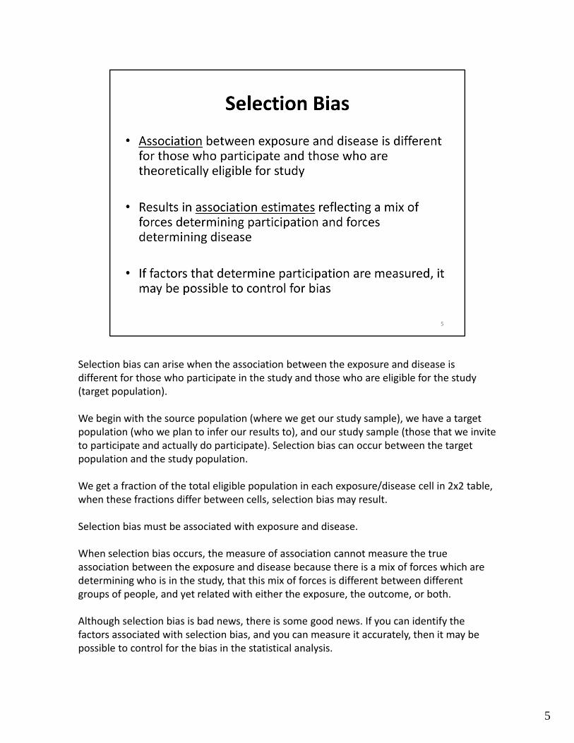
Selection bias can arise when the association between the exposure and disease is different for those who participate in the study and those who are eligible for the study (target population).

We begin with the source population (where we get our study sample), we have a target population (who we plan to infer our results to), and our study sample (those that we invite to participate and actually do participate). Selection bias can occur between the target population and the study population.

We get a fraction of the total eligible population in each exposure/disease cell in 2x2 table, when these fractions differ between cells, selection bias may result.

Selection bias must be associated with exposure and disease.

When selection bias occurs, the measure of association cannot measure the true association between the exposure and disease because there is a mix of forces which are determining who is in the study, that this mix of forces is different between different groups of people, and yet related with either the exposure, the outcome, or both.

Although selection bias is bad news, there is some good news. If you can identify the factors associated with selection bias, and you can measure it accurately, then it may be possible to control for the bias in the statistical analysis.

5

6

Let’s consider a series of diagrams to better understand selection bias.

Red symbols reflect a diseased case and blue symbols reflect a non‐diseased control.

If our sample is unbiased, we should see the same prevalence of disease (red symbols) in target population and study sample.

Referring to the diagram, the red shapes represent people with disease. The blue shapes represent people without disease. There are three different shapes, cylinders, triangles, and crosses. The big circle represents the general population. In the big circle, there are 20 crosses, 75% of which have disease and so are red, there are 20 triangles, 25% of which have the disease, and 12 cylinders, half of which have the disease.   We can think of the shapes as high, medium, and low risk subsets.

Now let’s select participants from the big circle and count them in the small circle, which is our study population. We sampled 4 crosses, 4 triangles, and 4 cylinders. Fortunately, the distribution of red and blue shapes is the same as the general population. That means, our study population was selected without bias.

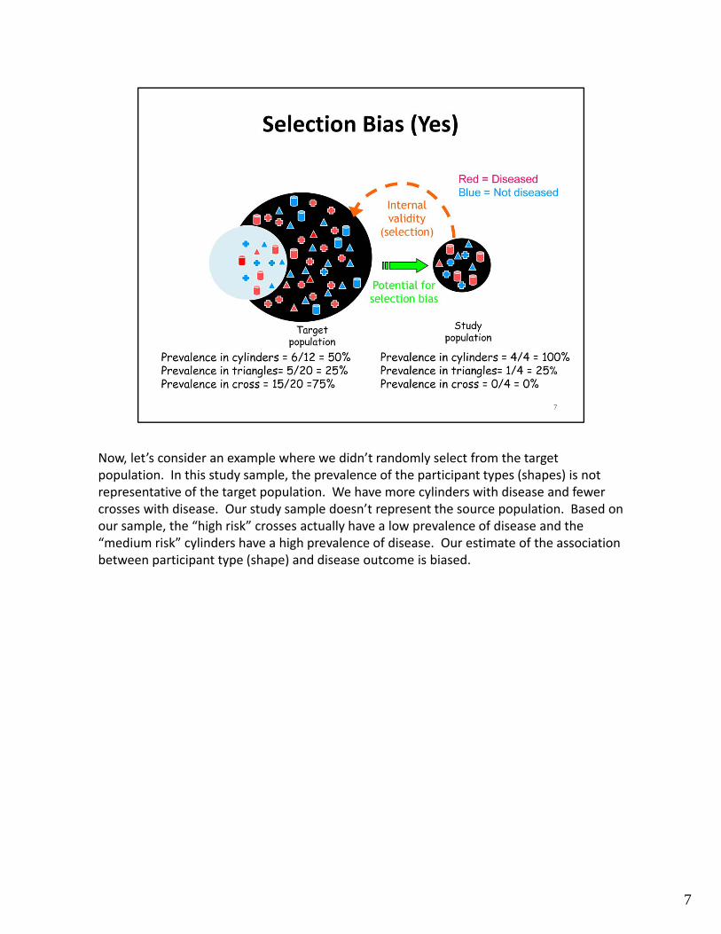
Now, let’s consider an example where we didn’t randomly select from the target population.  In this study sample, the prevalence of the participant types (shapes) is not representative of the target population.  We have more cylinders with disease and fewer crosses with disease.  Our study sample doesn’t represent the source population.  Based on our sample, the “high risk” crosses actually have a low prevalence of disease and the “medium risk” cylinders have a high prevalence of disease.  Our estimate of the association between participant type (shape) and disease outcome is biased.

7

Now, let’s consider some common sources of selection bias.  We will first consider self‐selection or membership bias.

Self‐selection can be subtle and tricky to identify. Bias can be introduced when characteristics of an individual leads them to select or engage (consciously or unconsciously) in certain health behaviors. Not necessarily self‐selecting to a group, but a behavior which affects exposure.

When assessing for self‐selection bias, consider the characteristics of the person. Individuals may select themselves into certain occupations or choose behaviors because of certain personal characteristics.  For example, individuals need to have a certain level of good health to jog and therefore, this selection criteria could impact your assessment of the association between jogging and heart disease where non‐joggers are less healthy and not able to participate in jogging.

Another source of selection bias relates to the “healthy worker effect”.  Keep in mind that those who are occupationally exposed may have decreased risk of disease because they must have a certain level of health to work. To address this source of selection bias, we typically use another occupational group as a comparison instead of the general population (includes workers and non‐workers).  Remember, the general population has people who are on disability, have mental illness, are excessively old, etc. 

The effect of self‐selection bias can go towards or away from the null, so you have to look 

8

at each context to decide the direction of the bias.

8

Note that in practice, self‐selection or membership bias is difficult to avoid.  To minimize the potential for self‐selection or membership bias, we can choose comparison groups with the same selection pressures or probabilities to try to balance the groups from the beginning.

It is important to keep in mind that self‐selection or membership bias cannot be completely avoided in observational studies given that the exposures and behaviors are not assigned at random; instead, participants make these selections.  We can, however, adjust for known and measured factors that are associated with self‐selection to have certain behaviors or exposures.

Note that self‐selection and membership bias can only be avoided if exposures are assigned at random, through an experimental clinical trial.  With randomization, individuals do not choose their exposures, but instead, exposures are assigned at random and therefore, are balanced between groups.

9

Let’s consider an example of self‐selection in more detail.

In our jogging example, assume that we were studying the effects of jogging on coronary heart disease (CHD).  To address this question, we compared the incidence of CHD in a sample of joggers to the incidence of CHD in a sample of individuals from the general population who did not exercise regularly.

Because joggers are more likely to eat a healthy diet – which is associated with lower rates of coronary heart disease, it will be difficult to separate the effect jogging has on coronary heart disease and eating a diet low in cholesterol unless you measure HDL and LDL levels in both groups and then can account for it in the analysis.  Also, members of the general population may not be healthy enough to participate in jogging, so the comparison between joggers and members of the general population who do not exercise regularly will reflect more than just the effect of jogging on the outcome.

10

Now, let’s consider another source of selection bias, namely, non‐response bias in case‐control studies.

Non‐response bias is another pervasive bias and is somewhat related to self‐selection bias. It is very rare to get 100% participation in studies. As participation rates decrease, can you predict the impact it may have on your study results? It may be helpful to find out reasons people chose not to participate, although this is difficult to assess in practice because people who don’t want to participate in the case‐control study are unlikely to participate in a different study to understand why they didn’t participate in the first place.

Keep in mind that people who agree to participate in the study may be different in terms of exposure or other important characteristics from those who do not agree.

The impact of selection bias may be to increase or decrease risk estimates depending on factors related to non‐response.

11

In practice, how can we determine if non‐response bias is present?  Note that we cannot simply compare response proportions between the cases and controls.  The response or participation proportions may be the same between the groups but the selection of the cases and controls relative to exposures may be biased (i.e., reasons associated with participation may differ even though the proportion participating is the same between cases and controls).  Alternatively, participation rates may be different between cases and controls but the sampling relative to exposure between the cases and controls is unbiased and therefore, non‐response bias is not present.

Bias occurs when participant cases have a different exposure frequency than non‐participant cases or participant controls have a different exposure frequency than non‐participant controls.  The selection must be related to both exposure and outcome in order to create bias. 

In practice, we can reduce the impact of non‐response bias by using methods to ensure high response proportions, such as using incentives to compensate participants for their time.

To assess the potential impact of non‐response bias, you should collect information about relevant patient characteristics, possibly collecting at least basic demographic characteristics on all (including non‐responders). You can also conduct a sensitivity analysis where you make different assumptions about the potential impact of bias and see what the potential impact on the estimate are.

12

Just knowing response proportions among cases and controsl is insufficient to address non‐response bias. You need to know the distribution of exposure among respondents and non‐respondents among both cases and controls. As your participation rate increases, the less impact non‐response bias will have on your results.

12

Let’s consider an example of non‐response bias. 

A case‐control study was conducted to determine the efficacy of Pap smears in reducing cervical cancer. 

The controls were identified by study personnel going through neighborhoods, knocking on doors, and soliciting participants.

On average, the sampling required knocking on 12 doors to find 1 control.  This is because no one was home at the time of the neighborhood canvassing.

13

So, suppose that being home was related to the likelihood of having had a Pap smear in the past five years. If women who were not at home were employed, and employed women were more likely to have health insurance, and therefore were more likely to have had a Pap smear than women staying at home, then the control group would have a higher proportion of women who had not had a Pap smear as a result of their insurance status. 

This non‐response of the controls with insurance could result in the control (non‐cancer controls) being less likely to have undergone Pap smears.  As a result, we could potentially underestimate the magnitude of the protective effect of the Pap smear on cervical cancer mortality because the non‐cases controls were less likely to be exposed to the Pap test as a result of the sampling method. 

14

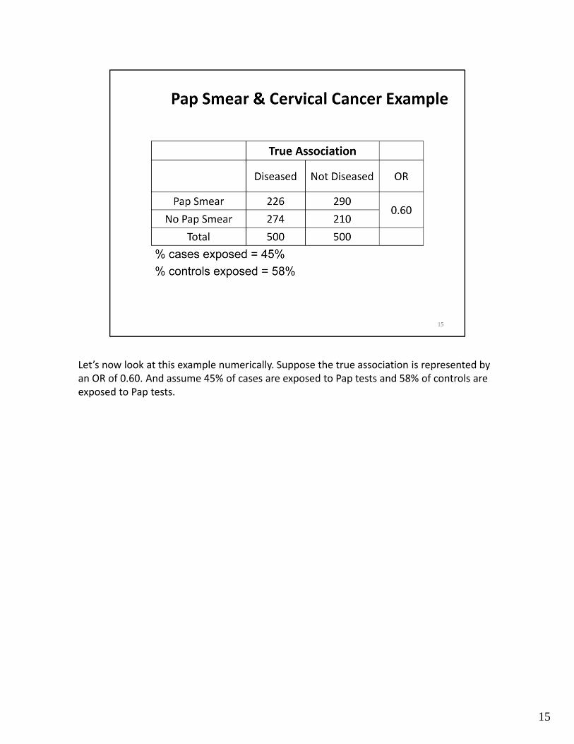
Let’s now look at this example numerically. Suppose the true association is represented by an OR of 0.60. And assume 45% of cases are exposed to Pap tests and 58% of controls are exposed to Pap tests.

15

Looking for the % of cases and controls exposed to be the same between what we observed and the non‐responders. If it was the same, even though the response proportion differed between cases and controls, there would be no bias.

In this case, even though only 80% of those approached agreed to participate, because the sampling was not related to disease state or exposure, we still have the result that 45% of cases received a Pap test and 58% of the controls were exposed to a Pap test, resulting in an OR of 0.59, essentially the same as the true association of 0.60.

If you have an 80% participation rate among cases and control and the exposure distribution remains the same among both cases and controls, the observed OR is essentially unchanged.

16

Now, let’s consider a case where we have an 80% participation rate among cases and controls, but the non‐response bias among controls (for example, less likely to sample controls who are exposed) reduces likelihood that control had a Pap smear by 10%.

In this case, the percent of cases with a Pap test remains at 45%; however, the percentage of controls with a Pap test is reduced from 58% to 48%.  As a result, the Odds Ratio changes from 0.60 to 0.89 and is biased towards the null.  With this type of biased sampling, we have underestimated the protective effect of a Pap test.

17

Now, let’s consider a case where we have a different response rate among cases and controls (e.g., 80% response among cases, 60% response among controls). In this case, the distribution of exposure among both cases and controls can be biased.

In this numeric example, the percent of cases with a Pap test increases from 45% to 50% and the percentage of controls with a Pap test is reduced from 58% to 48%.  As a result, the Odds Ratio changes from 0.60 to 1.1 and is biased.  In this example, cancer cases are associated with a higher odds of Pap test (OR > 1).

18

There is a type of bias in cohort studies called loss to follow‐up bias, which is similar to non‐response bias in case‐control studies. You can’t determine it’s presence by calculating participation rates among the exposed and non‐exposed groups alone because the bias can be present if follow‐up proportions are equal or bias could be absent if follow‐up proportions are unequal.  The presence of bias depends whether the disease incidence between exposed and unexposed differs between those remaining in the study versus those who are lost to follow‐up.

19

If the incidence of the outcome is different among exposed who are followed, compared to those who are lost, or among unexposed who are followed compared to those who are lost, then a biased risk estimate will result.  Again bias arises when the missing information or sampling differs by both exposure and outcome.

Strategies that are used to minimize loss to follow‐up bias include the use of incentives at enrollment and throughout the course of the study, as well as maintaining contact with the participants throughout the course of the study. 

In order to fully investigate the impact of bias, you need to know the proportion of those who experienced the outcome in both the followed and lost groups; however, if you knew whether the participant experienced the outcome, they wouldn’t be lost to follow‐up. Of course the best thing to do is try your best to follow‐up with each and every participant. Otherwise, you can try to compare the followed group and lost group by known characteristics and try to predict the effect on the study results.

20

21

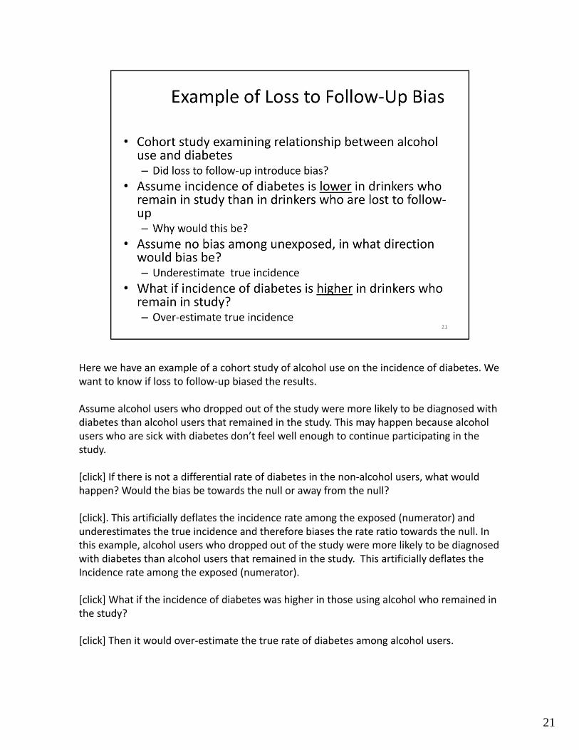
Here we have an example of a cohort study of alcohol use on the incidence of diabetes. We want to know if loss to follow‐up biased the results. 

Assume alcohol users who dropped out of the study were more likely to be diagnosed with diabetes than alcohol users that remained in the study. This may happen because alcohol users who are sick with diabetes don’t feel well enough to continue participating in the study. 

[click] If there is not a differential rate of diabetes in the non‐alcohol users, what would happen? Would the bias be towards the null or away from the null?

[click]. This artificially deflates the incidence rate among the exposed (numerator) and underestimates the true incidence and therefore biases the rate ratio towards the null. In this example, alcohol users who dropped out of the study were more likely to be diagnosed with diabetes than alcohol users that remained in the study.  This artificially deflates the Incidence rate among the exposed (numerator).

[click] What if the incidence of diabetes was higher in those using alcohol who remained in the study? 

[click] Then it would over‐estimate the true rate of diabetes among alcohol users.

The last form of selection bias we’re going to discuss is Berkson’s bias. This was named after Joseph Berkson who  described how cases who were hospitalized were different from cases of the same disease who were not hospitalized. This may happen if there is a combination of factors which increase the probability of a person being hospitalized. These factors could be biologic or sociologic. 

These factors may affect controls as well, depending on the control selection. Like all biases, its difficult to address unless you know it’s present.

22

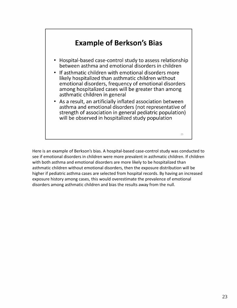
Here is an example of Berkson’s bias. A hospital‐based case‐control study was conducted to see if emotional disorders in children were more prevalent in asthmatic children. If children with both asthma and emotional disorders are more likely to be hospitalized than asthmatic children without emotional disorders, then the exposure distribution will be higher if pediatric asthma cases are selected from hospital records. By having an increased exposure history among cases, this would overestimate the prevalence of emotional disorders among asthmatic children and bias the results away from the null. 

23

In summary, we have learned that biases are a primary source of error in observational epidemiologic research.  Biases can be either conscious or unconscious.  To prevent or limit sources of bias, we need to consider whether the study design is appropriate for the hypotheses under investigation.  In our design and implementation, we need to use appropriate sample selection methods that are both valid and reliable.  It is also important to learn from other studies, and avoid reported sources of bias that have arisen with other studies. 

24