Part I (Electric and electromagnetic Methods)

Prof. Dr. Adel Kamel

1

Part I

(Electric and electromagnetic

Methods)

Prof. Dr. Adel Kamel Mohamed


2

DIRECT CURRENT RESISTIVITY TECHNIQUE

Since students have taken the basic principle of electric methods before in

physics department, we will continue learning measurement and interpretation

with reviewing some basic points. Geophysical resistivity techniques are

based on the response of the earth to the flow of electrical current. In

these methods, an electrical current is passed through the ground and two

potential electrodes allow us to record the resultant potential difference

between them, giving us a way to measure the electrical resistance of the

subsurface material. The apparent resistivity is then a function of the measured

resistance (ratio of potential to current) and the geometry of the electrode

array. Depending upon the survey geometry, the apparent resistivity data are

plotted as 1-D soundings, 1-D profiles, or in 2-D cross-sections (that will

discuss later ) in order to look for anomalous regions.

In the shallow subsurface, the presence of water controls much of the

conductivity variation. Measurement of resistivity (inverse of conductivity) is,

in general, a measure of water saturation and connectivity of pore space. This

is because water has a low resistivity and electric current will follow the path

of least resistance. Increasing saturation, increasing salinity of the

underground water, increasing porosity of rock (water-filled voids) and

increasing number of fractures (water-filled) all tend to decrease

measured resistivity. Increasing compaction of soils or rock units will

expel water and effectively increase resistivity. Air, with naturally high

resistivity, results in the opposite response compared to water when filling

voids. Whereas the presence of water will reduce resistivity, the presence of

air in voids should increase subsurface resistivity. Also presence of

hydrocarbon increases the resistivity reading.

Resistivity measurements are associated with varying depths depending

on the separation of the current and potential electrodes in the survey, and


3

can be interpreted in terms of a lithologic and/or geohydrologic model of the

subsurface. Data are termed apparent resistivity because the resistivity values

measured are actually averages over the total current path length but are

plotted at one depth point for each potential electrode pair. Two dimensional

images of the subsurface apparent resistivity variation are called

pseudosections. Data plotted in cross-section is a simplistic representation of

actual, complex current flow paths. Computer modeling can help interpret

geoelectric data in terms of more accurate earth models.

Classification of Materials according to Resistivities Values

a) Materials which lack pore spaces will show vey high resistivity such as

massive limestone and most igneous and metamorphic (granite, basalt)

b) Materials whose pore space lacks water will show high resistivity such as

dry sand and gravel. Also pores filled with petroleum will show high

resistivity

c) Materials whose connate water is clean (free from salinity) will show high

resistivity such as clean sand or gravel , even if water saturated.

d) most other materials will show medium or low resistivity, especially if clay

is present such as clay soil and weathered rock.

Factors which control the Resistivity

(1) Geologic Age

(2) Salinity.

(3) Free-ion content of the connate water.

(4) Interconnection of the pore spaces (Permeability).

(5) Temperature.

(6) Porosity.

(7) Pressure

(8) Depth

Resistivity survey instruments:


4

a- High tension battery pack (source of current).

b- Four metal stakes.

c- Milliammeter.

d- Voltmeter.

e- Four reels of insulated cable.

Field considerations for DC Resistivity

1- Good electrode contact with the earth

- Wet electrode location.

- Add Nacl solution or bentonite

2- Surveys should be conducted along a straight line whenever possible .

3- Try to stay away from cultural features whenever possible .

- Power lines

- Pipes

- Ground metal fences

- Pumps

Sources of Noise

There are a number of sources of noise that can effect our measurements of

voltage and current.

1- Electrode polarization.

A metallic electrode like a copper or steel rod in contact with an electrolyte

groundwater will generate a measurable contact potential. For DC Resistivity,

use non polarizing electrodes. Copper and copper sulfate solutions are

commonly used.

2- Telluric currents.

Naturally existing current flow within the earth. By periodically reversing the

current from the current electrodes or by employing a slowly varying AC

current, the affects of telluric can be cancelled.


5

3- Presence of nearby conductors. (Pipes, fences)

Act as electrical shorts in the system and current will flow along these

structures rather than flowing through the earth.

4- Low resistivity at the near surface.

If the near surface has a low resistivity, it is difficult to get current to flow

more deeply within the earth.

5- Near- electrode Geology and Topography

Rugged topography will act to concentrate current flow in valleys and disperse

current flow on hills.

6- Electrical Anisotropy.

Different resistivity values will be obtained if measured parallel to the bedding

plane hen wcompared to perpendicular to it .

7- Instrumental Noise .

8- Cultural Feature.

Electric current flow in a half-space

1 Potential of a single current electrode

In the lab, the electrical resistivity of a rock sample can be measured by

placing flat electrode plates on each side of a rectangular sample. In this

geometry the electric current flow is parallel and the simple equation

derived in C1 can be used to compute the resistivity, ρ from the measured

resistance (R). However this approach is not practical for the measuring

the Earth, since we cannot inject current from large plates. Thus we must

consider the electric current flow from a simple electrode (metal spike).


6

Consider an electric current, I, flowing from an electrode. The air has a

very high electrical resistivity, so all current flows in the Earth. From

symmetry arguments, the current spreads out uniformly in all directions.

Now consider a shell of rock, with radius, r, and thickness dr. The voltage

(potential) drop across the shell is ΔV

The resistance of the hemispherical shell,

Rearranging and taking limits gives

(the minus sign accounts for the fact that V decreases with r)

To compute the potential, V, apply the boundary condition that V = 0 when r =

∞ and integrate to

give:


7

Thus surfaces of equal potential (equi potentials) will be hemispheres centered

on the electrode. Note that the electric current flow is at right angles to the

equipotential. (just like for gravity.

The voltage between the electrodes A and B is defined as ΔVAB = VA-VB

Using the above result

where rA and rB are the distances from the current electrode to the potential

electrodes A and B respectively. Rearranging this equation gives

Note that this is essentially Ohms Law with a geometric factor added.

2 Potential of two-current electrodes, definition of apparent resistivity

A more realistic situation uses two current electrodes. Current is injected

through one electrode and withdrawn through the other.


8

To compute the potential at electrode P1, we can simply add the potentials

generated by the two current electrodes C1 and C2.

However, to measure a voltage, we need two potential electrodes to

connect to a voltmeter. Consider the arrangement of electrodes shown

below.

The voltage difference measured between electrodes P1 and P2 is given by

Now let us make the geometry of the array simple, with the 4 electrodes

separated by a distance a. Then we have r1 = r4 = a and have r2 = r3 = 2a


9

This represents a solution to a forward problem i.e. for a model of the Earth

resistivity, ρ) we can predict the value of ΔV that will be observed in a

geophysical survey. Simple rearrangement gives us a solution to the

corresponding inverse problem.

The electrical resistivity methods is commonly used therefore to map

lateral and vertical changes in geological (or man-made) materials. The

method may also used to:

1. assess the quality of rock/soil masses in engineering terms;

2. determine the depth to the water table (normally in arid or semi-arid

areas);

3. map the saline/fresh water interface in coastal regions;

4. locate economic deposits of sand and gravel; and

5. locate buried features such as cavities, pipelines, clay-filled sink holes

and buried channels. The electrical resistivity of a material is defined as the

resistance offered by a unit cube of that material to the flow of electrical

current between two opposite faces. Most common rock forming minerals are

insulators, with the exception of metalliferous minerals which are usually good

conductors. In general, therefore, rocks and soils conduct electricity by

electrolytic conduction within the water contained in their pores, fissures, or

joints. It follows that the conductivity of rocks and soils is largely dependent

upon the amount of water present, the conductivity of the water, and the

manner in which the water is distributed within the material (i.e., the porosity,

degree of saturation, degree of cementation, and fracture state).

These factors are related by Archie’s empirical equation (Archie 1942):

where = resistivity of the rock or soil, = resistivity of the pore water, n =

porosity, s degree of saturation, 1=2, m = 1.3-2.5, and a = 0.5-2.5.


10

The manner in which the water is distributed in the rock determines the factor

m (cementation factor) which for loose (uncemented sands) is about 1.3 (Van

Zijl 1978). The validity of Archie’s equation is, however, dependent on various

factors such as the presence or absence of clay minerals (Griffiths 1946).

Guyod (1964) gives a simplified version of Archie’s equation:

where = resistivity of the rock/soil, = resistivity of the pore water, and n =

porosity.

Because the conduction of electrical current through the pore water is

essentially electrolytic, the conductivity of the pore water must be related to

the amount and type of electrolyte within it. Figure given below shows the

relation between the salinity of the pore water and the measured resistivity for

materials with different porosities. As the salinity of the pore water increases,

there is a significant decrease in measured resistivity. The above relationships

suggest that the more porous (or the more fissured/jointed) the soil or rock is,

the lower is its resistivity. Thus, in general, crystalline rocks such as igneous

rocks which exhibit a low porosity, have a high resistivity compared with the

more porous sedimentary rocks such as sandstones. Clay-bearing rocks and

soils will tend to have lower resistivities than non clay-bearing rocks and soils.

These generalizations are reflected in the typical resistivity values for different

soil and rock types given in the Table given below.


11

Table: Typical electrical resistivity values for different soil and rock

types

* Values from Dohr (1975).

† Values from Sowers and Sowers (1970).

OPERATION

Figure is a schematic diagram showing the basic principle of D.C. resistivity

measurements. Two short metallic stakes (electrodes) are driven about 1 foot

into the earth to apply the current to the ground. Two additional electrodes are

used to measure the earth voltage (or electrical potential) generated by the

current. Depth of investigation is a function of the electrode spacing. The

greater the spacing between the outer current electrodes, the deeper the

electrical currents will flow in the earth, hence the greater the depth of

exploration.


12

Figures show different types pf arrays

Wenner array

=

I

Vaa 2

Schlumberger array

I

VaLa

−=

42

2


13

Dipole dopole array

( )( )I

Vannna

++= 21


14

Porous-pot non-polarizing electrodes

SURVEY DESIGN

Two categories of field techniques exist for conventional resistivity analysis of

the subsurface. These techniques are vertical electric sounding (VES), and

Horizontal Electrical Profiling (HEP).


15

1- Vertical Electrical Sounding (VES).

The objective of VES is to deduce the variation of resistivity with depth below

a given point on the ground surface and to correlate it with the available

geological information in order to infer the depths and resistivities of the layers

present.

In VES, with wenner configuration, the array spacing “a” is increased by

steps, keeping the midpoint fixed (a = 2 , 6, 18, 54…….) .

In VES, with schlumberger, The potential electrodes are moved only

occasionally, and current electrode are systematically moved outwards in steps

AB > 5 MN.

2- Horizontal Electrical profiling (HEP) .

The objective of HEP is to detect lateral variations in the resistivity of the

ground, such as lithological changes, near- surface faults…… .

In the wenner procedure of HEP , the four electrodes with a definite array

spacing “a” is moved as a whole in suitable steps, say 10-20 m. four electrodes

are moving after each measurement.

In the schlumberger method of HEP, moving all four electrodes together

after each measurement.

Multiple Horizontal Interfaces

For Three layers resistivities in two interface case, four possible curve types

exist.

1- Q – type ρ1> ρ2> ρ3

2- H – Type ρ1> ρ2< ρ3

3- K – Type ρ1< ρ2> ρ3

4- A – Type ρ1< ρ2< ρ3


16

In four- Layer geoelectric sections, there are 8 possible relations:

ρ1> ρ2< ρ3< ρ4 HA Type

ρ1> ρ2< ρ3> ρ4 HK Type

ρ1< ρ2< ρ3< ρ4 AA Type

ρ1< ρ2< ρ3> ρ4 AK Type

ρ1< ρ2> ρ3< ρ4 KH Type

ρ1< ρ2> ρ3> ρ4 KQ Type

ρ1> ρ2> ρ3< ρ4 QH Type

ρ1> ρ2> ρ3> ρ4 QQ Type

Quantitative VES Interpretation: Master Curves

Layer resistivity values can be estimated by matching to a set of master curves

calculated assuming a layered Earth, in which layer thickness increases with

depth. For two layers, master curves can be represented on a single plot.


17

Master curves: log-log plot with ρa / ρ1 on vertical axis and a / h on horizontal

(h is depth to interface)

Plot smoothed field data on log-log graph transparency.

Overlay transparency on master curves keeping axes parallel.

Note electrode spacing on transparency at which (a / h=1) to get interface

depth.

Note electrode spacing on transparency at which (ρa / ρ1 =1) to get

resistivity of layer 1.

Read off value of k to calculate resistivity of layer 2 from equation given

above:

Quantitative VES Interpretation: Inversion

Curve matching is also used for three layer models, but book of many more

curves. Recently, computer-based methods have become common:

forward modeling with layer thicknesses and resistivities provided by

user


18

inversion methods where model parameters iteratively estimated from

data subject to user supplied constraints as given by (Barker, 1992).

Start with model of as many layers as data points and resistivity equal to

measured apparent resistivity value.

Calculated curve does not match data, but can be perturbed to improve fit.

Limitations of Resistivity Interpretation

1- Principle of Equivalence (non uniqeness).


19

If we consider three-lager curves of K (ρ1< ρ2> ρ3 ) or Q type (ρ1> ρ2> ρ3)

we find the possible range of values for the product T2= ρ2 h2 Turns out to be

much smaller. This is called T-equivalence. H = thickness, T : Transverse

resistance it implies that we can determine T2 more reliably than ρ2 and h2

separately. If we can estimate either ρ2 or h2 independently we can narrow

the ambiguity. Equivalence means several models produce the same

results. Ambiguity in physics of 1D interpretation such that different layered

models basically yield the same response.

2- Principle of Suppression.

This states that a thin layer may sometimes not be detectable on the field

graph within the errors of field measurements. The thin layer will then be

averaged into on overlying or underlying layer in the interpretation. Thin

layers of small resistivity contrast with respect to background will be missed.

Thin layers of greater resistivity contrast will be detectable, but equivalence

limits resolution of boundary depths, etc.

The delectability of a layer of given resistivity depends on its relative thickness

which is defined as the ratio of Thickness/Depth.

Comparison of Wenner and Schlumberger sounding

(1) In Sch. MN ≤ 1/5 AB

Wenner MN = 1/3 AB

(2) In Sch. Sounding, MN are moved only occasionally.

In Wenner Soundings, MN and AB are moved after each measurement.

(3) The manpower and time required for making Schlumberger soundings are

less than that required for Wenner soundings.

(4) Stray currents that are measured with long spreads effect

measurements with Wenner more easily than Sch.

(5) The effect of lateral variations in resistivity are recognized and corrected

more easily on Schlumberger than Wenner.


20

Disadvantages of Wenner Array

1. All electrodes must be moved for each reading

2. Required more field time

3. More sensitive to local and near surface lateral variations

4. Interpretations are limited to simple, horizontally layered structures

Advantages of Schlumberger Array

1. Less sensitive to lateral variations in resistivity

2. Slightly faster in field operation

3. Small corrections to the field data

Disadvantages of Schlumberger Array

1. Interpretations are limited to simple, horizontally layered structures

2. For large current electrodes spacing, very sensitive voltmeters are required.

Advantages of Resistivity Methods

1. Flexible

2. Relatively rapid. Field time increases with depth

3. Minimal field expenses other than personnel

4. Equipment is light and portable

5. Qualitative interpretation is straightforward

6. Respond to different material properties than do seismic and other methods,

specifically to the water content and water salinity

Disadvantages of Resistivity Methods

1- Interpretations are ambiguous, consequently, independent geophysical and

geological controls are necessary to discriminate between valid alternative

interpretation of the resistivity data ( Principles of Suppression & Equivalence)

2- Interpretation is limited to simple structural configurations.

3- Topography and the effects of near surface resistivity variations can mask

the effects of deeper variations.


21

4- The depth of penetration of the method is limited by the maximum electrical

power that can be introduced into the ground and by the practical difficulties of

laying out long length of cable. The practical depth limit of most surveys is

about 1 Km.

5. Accuracy of depth determination is substantially lower than with

seismic methods or with drilling.

Lateral inhomogeneities in the ground affect resistivity measurements in

different ways: The effect depends on

The size of inhomogeneity with respect to its depth

2. The size of inhomogeneities with respect to the size of electrode array

3. The type of electrode array used

4. The geometric form of the inhomogeneity

6. The orientation of the electrode array with respect to the strike of the

inhomogeneity

We have to note the following:

Apparent Resistivity:

Instrument readings (current and voltage) are generally reduced to "apparent

resistivity" values. The apparent resistivity is the resistivity of the

homogeneous half-space which would produce the observed instrument

response for a given electrode spacing. Apparent resistivity is a weighted

average of soil resistivities over the depth of investigation. For soundings a

log-log plot of apparent resistivity versus electrode separation is obtained. This

is sometimes referred to as the "sounding curve."

Modeling:

Resistivity data is generally interpreted using the "modeling" process: A

hypothetical model of the earth and it's resistivity structure (geoelectric

sections) is generated. The theoretical electrical resistivity response over that

model is then calculated. The theoretical response is then compared with the


22

observed field response and differences between observed and calculated are

noted. The hypothetical earth model is then adjusted to create a response

which more nearly fits the observed data. When this iterative process is

automated it is referred to as "iterative inversion" or "optimization."

Uniqueness

Resistivity models are generally not unique; i.e., a large number of earth

models can produce the same observed data or sounding curve. In general,

resistivity methods determine the "conductance" of a given stratigraphic layer

or unit. The conductance

is the product of the resistivity and the thickness of a unit. Hence that layer

could be thinner and more conductive or thicker and less conductive, and

produce essentially the same results. Hence constraints on the model, from

borehole data or assumed unit resistivities, can greatly enhance the

interpretation.

Geoelectric" cross section

The end product from a D.C. resistivity survey is generally a "geoelectric"

cross section showing thicknesses and resistivities of all the geoelectric units or

layers. If borehole data or a conceptual geologic model is available, then a

geologic identity can be assigned to the geoelectric units. A two-dimensional

geoelectric section may be made up of a series of one-dimensional

soundings joined together to form a two-dimensional view section, or it

may be a continual two dimensional modeling cross section (using multi

electrode system). The type of section produced depends on the acquisition

parameters and the type of processing applied to the data.

Figure is a two dimensional modeling geoelectric section from a dipole-

dipole survey in Alaska. The resistivity survey, part of a water resources

investigation, was conducted in order to identify fracture zones with increased


23

porosity. The geophysical objective was to locate conductive fracture zones in

the more resistive bedrock.

APPLICATIONS

Electrical resistivity of soils and rocks correlates with other soil/rock properties

which are of interest to the geologist, hydrogeologist, geotechnical engineer

and/or quarry operator.

D.C. resistivity techniques may be used to map lateral changes and identify

near-vertical features (e.g., fracture zones), or they may be used in the

sounding mode (e.g., Schlumberger soundings) to determine depths to

geoelectric horizons (e.g., depth to saline groundwater).

Common applications of the D.C. resistivity method include

• estimating depth to bedrock, to the water table, or to other geoelectric

boundaries, and

• mapping and/or detecting other geologic features. D.C. resistivity and

electromagnetic (EM) techniques both measure electrical properties of the

earth, and hence both are used for many of the same applications.

Conductivity, which is often reported by EM instruments, is the reciprocal of

resistivity.


24

Basic EM theory

Electromagnetic theory was first comprehended by Maxwell who

recognized that Ohm’s law, Faraday’s law, and Amperes’s law were all

part of a great whole, that now being called Maxwell’s equations. These

equations are the quintessence of the development of electromagnetic

theory. Further development was only a matter of performing the

appropriate mathematical manipulations. Maxwell’s field equations for a

homogeneous isotropic medium, assuming a time dependence of the type eiwt

and a charge free space, are;

= −E B t / (2.1)

= +H J D t / (2.2)

=. B 0 (2.3)

=. D 0 , (2.4)

where E is the electric field intensity (V/m), H is the magnetic field

intensity (A/m), B is the magnetic induction (W/m 2 ), D is the

displacement current (C/m 2 ), and J is the current density (A/m 2).

To relate Maxwell’s equations to properties of the subsurface, the

constitutive equations must be used

D E= . (2.5)

B H= . (2.6)

J E= . , (2.7)

where )/( mF is the dielectric constant or electrical permitivity, is the

magnetic permeability ( / 0

74 10= − H m in free space), ( / )S m is the

electrical conductivity. In most materials, and do not differ

appreciably from the values of 0 and 0 in free space. A combination of

Maxwell’s and constitutive equations form a single characteristic of the

medium referred to as the wave number which then determines the


25

behaviour of the EM field. Reformulation of Maxwell equations (2.1 and 2.2)

in terms of the magnetic and electrical field strengths, gives the following;

= +H Et

E

( ) (2.8)

= −Et

H

( ) . (2.9)

The ratio of electric field strength to the magnetic field strength is known

as the Cagniard impedance or wave impedance (units in ohm) and is given

by

( )ZEx

Hyw

T= = =

0

1 2

3

1 22

10 5

//

. (2.10)

Re-arranging the above equation, the apparent resistivity in a

homogeneous medium is

a TEx

Hy= 0 2

2

. . (2.11)

The depth z at which the amplitude of the field has been attenuated by 1/e

or 0.37 of its value at the surface of the medium is called skin depth and is

given by

( )

( ) ( )

= = =

1 2 2503

1 2

1 2

real k w wT m

. .

/

/. (2.12)

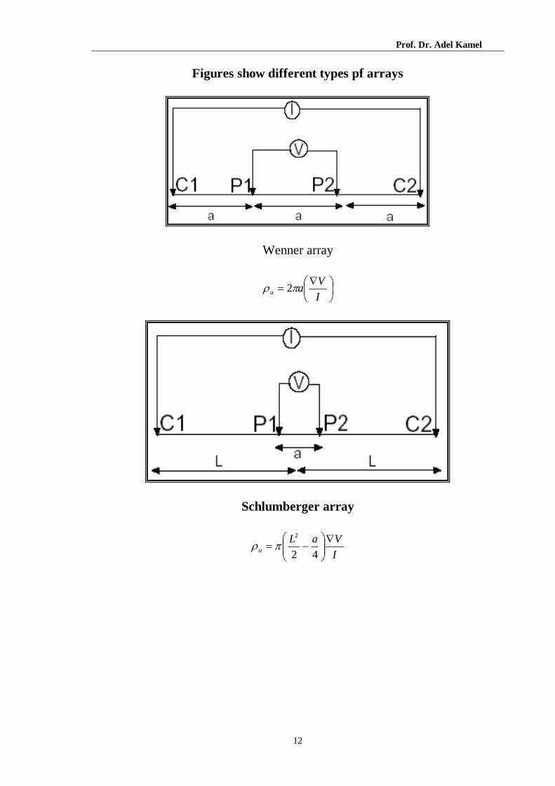
The effect of conductivity on penetration depth (Fig. ) can be explained

physically as follow (Zhadanov and Keller, 1994): as an electromagnetic field

penetrates a conductor, its energy is expended on the vibration of free

electrical charge carriers present in the conductor. The vibration excited by the

electromagnetic field represents conversion of the energy of electromagnetic

field to heat. As a result, the field in a conductor loses energy rapidly as it

travels, and is attenuated. When an electromagnetic field travels into an

extensive conductor, its energy is almost entirely lost in a zone near the entry

surface; this zone is like a skin protecting the interior of the conductor from

penetration by electromagnetic field, and hence the name skin effect. In an


26

insulator, there are no free charge carriers to vibrate and extract energy from

the electromagnetic field, and so, the field can propagate to greater distance.

Figure: Wave numbers as a function of frequency and resistivity. A scale for

converting wave numbers to radian wave lengths or skin depths is shown on

the right hand side (Keller and Frischknecht, 1966).

The physical meaning of Frequency domain electromagnetic methods

The physical meaning is that a transmitter coil radiates an

electromagnetic field which induces eddy currents in the subsurface. The

eddy currents, in turn, induce a secondary electromagnetic field. The

secondary field is then intercepted by a receiver coil. The voltage

measured in the receiver coil is related to the subsurface conductivity.

These conductivity readings can then be related to subsurface conditions.

Figure presents a schematic drawing of EM operating principles.

The conductivity of geologic materials is highly dependent upon the water

content and the concentration of dissolved electrolytes. Clays and silts

typically exhibit higher conductivity values because they contain a relatively


27

large number of ions. Sands and gravels typically have fewer free ions in a

saturated environment and, therefore, have lower conductivities.

Figure: Schematic Drawing of Electromagnetic Operating Principles

Basic theory of magnetotelluric method

The magnetotelluric field can be defined as the time-varying portion of

the earth’s magnetic field which induces current flow in the earth. The

source of the MT fields is natural electromagnetic energy from distant

transient sources in the ionosphere. This energy is utilised to probe the

resistivity structure of the earth’s interior from depths of tens of meters to

many hundreds of kilometres. The external magnetic fields penetrate the

ground to induce electric fields and secondary magnetic fields. Then the

components of the electric and magnetic fields are measured on the

surface. The study of natural EM fields has shown that the amplitude of the

electric field component (E) is strongly dependent on local geology and can

vary by a factor of 20 over a distance of about 1 km (Yungul, 1996). On the


28

other hand, the magnetic field component (H) is very much less dependent on

local geology and seldom varies by more than a factor of 1.5 within the

distance of a few kilometres (Yungul, 1996). A typical average amplitude

spectrum of the magnetic variations shows a minimum at about 1 Hz (Fig. 2.1)

and allows the source field to be classified into two types of activities, one

above and the other below 1 Hz. This frequency (1 Hz) distinguishes two

kinds of activities with relative sources above and below 1 Hz.

Sources above 1 Hz

The electrical storms in the lower atmosphere are the main source of

fields of frequencies above 1Hz. It includes fields from lightning

associated with thunderstorms. The lightning signals are referred to as

“sferics” and attain their peaks in the early afternoon, their frequency

range being between 5 Hz and 30 MHz (Yungul, 1982). They propagate

around the world trapped in the waveguide formed between the ionosphere and

the earth’s surface. In the day time the waveguide width is 60 km increasing to

90 km during the night time. This wave guide at large distance from the source

is converted into a plane wave of variable frequency. There are three storm

centres in the equatorial regions (Brazil, central Africa, and Malaysia).

These centres have an average of 100 storms; their geographic

distribution is such that during any hour of the day there is possibly a

storm in progress in one of the centres. This is in addition to small areas

within these centres which average more than 200 stormy days per year.

These MT fields penetrate the earth’s surface to produce the telluric currents.

The amplitude of the induced current has peaks at distinct frequencies (e.g. the

Schumann resonance; 8, 14, 20, 26, 32 Hz) since the wave-guide absorbs

energy at these frequencies to become enhanced (Jiracek et al., 1995). Man-

made power distribution systems are other minor sources of signals which are


29

generally localised and restricted, to 50 or 60 Hz and subsequent harmonics.

However, the total energy available from these frequencies is very small.

Sources below 1 Hz

The complex interaction between the solar wind (charged particles

emanating from the sun) with the earth’s magnetic field and atmosphere

is the main cause of the natural EM field below 1 Hz. When ionised

particles moving outward from the sun encounter the earth’s magnetosphere,

the ionised particles produce protons and electrons. When the protons and

electrons encounter the terrestrial magnetic field, they are deflected in opposite

directions and thus current systems are produced with their own secondary

magnetic field to oppose the earth’s field which appears to change at a level of

a few gammas at a boundary called the “magnetopause” which is the outer

boundary of the earth’s magnetosphere. This complex interaction results in

what is called micropulsations which are the main source of fields in the range

of frequency of 0.00167 to 5 Hz (Yungul, 1996). Their amplitudes depend on

solar activity, latitude, frequency, season, local and universal times, and local

geology. Depending on their continuity and periods, the micropulsations are

classified as continuous pulsation (regular) and irregular pulsation (Parkinson,

1983). Continuous pulsations occur mostly during the daytime forming wave

trains that last for tens of minutes. Their amplitudes tend to peak in the early

afternoon (local mean time) and diminish during the night. Irregular pulsations

occur mostly during night time with wave trains that are of limited duration and

a period range of about 40 to 120 seconds (frequency range 0.025 to 0.00833

Hz). In areas where industrial electromagnetic noise is too high for any

meaningful exploration during day time, irregular pulsations are very useful.


30

Figure: A schematic drawing depicting the magnetotelluric field

equipment.

Transient electromagnetic (TEM) method

Basic principles

The transient electromagnetic (TEM) method is an inductive method that

utilises strong current which is passed through a rectangular loop

commonly laid on the surface of the ground. The flow of this current in

the surface loop will create a magnetic field that spreads out into the

ground in the form of a primary magnetic field and induces eddy currents

in the subsurface. When the current is abruptly terminated, this primary

magnetic field is time varying and in accordance with Faraday’s law,

there will be an electromagnetic induction during this time. This

electromagnetic induction in turn results in eddy current flow in the

subsurface. The intensity of these currents at a certain time and depth

depends on ground resistivity (Kaufman and Keller, 1983), in other

words, the conductivity, size, and shape of subsurface conductor. The

voltage response, which is proportional to the time rate of change of the

secondary magnetic field created by the eddy currents, is measured. For

poor conductors, these initial voltages are large but the fields decay

rapidly. For good conductors, the initial voltages are smaller but the field


31

decays slowly. Nabighian (1979) has shown that at any given time after

switch off, this system of induced currents can be represented by a simple

current filament of the same shape as the transmitter loop, and moves outward

and downward with decreasing velocity and diminishing amplitude with time

(Figure.). This is known as the smoke ring.

Figure: System of equivalent current filaments at various times after

current interruption in the transmitter loop, showing their downward and

outward movement (after McNeill, 1990).

The velocity VZ with which the ring expands away from the transmitter, at a

time t is given by the equation (Nabighian, 1979)

Vt

Z =2

, (3.1)

and the diffusion depth, d, of the wave is given by

t

d2

2= . (3.2)

The depth of investigation is determined by the time interval after the

transmitter current is turned off and the subsurface conductivity

(equation 3.2). As the time increases, the current intensity migrates to

greater depths.

The current driven through the transmitter loop consists of equal periods

of on-time and off-time (Figure). The TDEM signal is measured during


32

the transmitter off time period only, i.e. in the absence of a primary field.

When the TEM response is plotted logarithmically against the logarithm of

time in a homogeneous medium, the response can be divided into three stages,

early stage (where the response is constant with time), an intermediate stage

(response shape is continually varying with time), and late stage (response is a

straight line).

Figure: Schematic diagram showing on and transmitter current linear

ramp turn-off time and receiver signal (after Swift, 1990).

In the early time stage of the transient process, the induced currents (Grant and

West, 1965) will be independent of the conductivity and firstly (i.e. at time

t=0) be confined to the surface of the conductor in such a way as to preserve

the normal component of the pre-existing primary magnetic field at the surface

of the conductor (Weaver, 1970). At this stage, the initial current distribution

is only a function of the size and shape of the conductor (Grant and West,

1965). In the subsurface, an inward diffusion of the current pattern later occurs

as a result of ohmic losses which leads to the region immediately inside the

conductor seeing a decreasing magnetic field and an induced emf that causes


33

new current to flow. This is the intermediate stage. This continues until a

stage is reached at which current distribution becomes more or less invariant

with time. The inductance and resistance of each current ring have reached

stabilised values and both the currents and their associated external magnetic

fields begin to decay with a time constant given by

=

a2

2, (3.3)

where a is the radius of an equivalent circular loop.

This is the late–time stage of the transient process.

TEM in homogeneous medium

The derivative of the vertical magnetic field, BZ as a function of time is given

by (McNeill, 1980)

( )( )

B

tM t

t= / /

/

/4 3 2

3 2

5 2. (3.4)

Re-arranging this equation by inversion, we have

( )

a

z

tt

M

tB=

•4

2

5

2 3/

, (3.5)

where M is the transmitter dipole moment,

BB

tz

• =

and a is the apparent resistivity of the ground.

TEM field measurements

In the TEM survey, the transmitter is connected to a loop of wire laid on

the ground. With the exception of the on time measuring system (UTEM

and INPUT), all TEM transmitters generate a bipolar waveform with a

ramp turn-off time as shown in Figure . The decaying voltage in the

receiver is measured when the transmitter is turned off which allows the

very small voltage to be measured without interference from the large

primary field. The receiver samples the amplitude of the transient decay

using a number of gates. The width of gates increases with time so the

early time gates are narrow in order to accurately measure the voltage


34

while the later gates, situated where the transient varies more slowly, are

much broader. This wider gate enhances the signal to noise ratio which

decreases with time as the amplitude of the signal decays.

The design of TEM survey depends on the depth of investigation

required. The practical limitation on the depth of investigation for TEM

system is determined by the maximum recording time, the time t at which

the signal decays to the noise level, the source moment and earth

resistivity. These independent parameters render the depth of investigation

difficult to quantify. Spies (1989) has studied the depth of investigation of

TEM survey; he has shown that in case of transmitter-receiver separation or

loop size less than the depth of investigation (near-zone) and induced voltage

measured with an induction coil, the depth of investigation is proportional to

the 1/5 power of the source moment and ground resistivity 5/1)( IA . On the

other hand, if the receiver is a magnetometer the depth of investigation is

proportional to the 1/3 power of the source moment and is no longer a function

of resistivity. In case of loop size greater than the depth of investigation (far-

zone), the depth of investigation for an induced voltage receiver is proportional

to the ¼ power of the source moment and resistivity and is inversely

proportional to the source-receiver separation (Spies, 1989). This analysis

gives the maximum depth of investigation based on detection of a buried layer.

The minimum depth, at which individual conductivity variations can be

resolved, is determined by the earliest sample time.

TEM loop configurations

The most common factor for designing all time domain techniques is the

fact that they all utilise either square shaped or rectangular as the

transmitter. Also a large transmitter loop offers a better capability for

depth penetration. These methods use either fixed- or moving-loop

configurations and measure the rate of decay of the secondary field when the


35

primary field is switched off. They are mostly used to investigate the variation

of conductivity with depth (resistivity sounding). A number of different loop

configurations are possible for TEM measurements, some being better

than others for specific geologic situations. They include the common

zero-offset (in-loop and single-loop), short offset (separated-loop or

soTEM) and the long-offset (loTEM) techniques. Figure 3.3 illustrates the

most common loop configurations. Brief descriptions of the most

commonly used TEM loop configurations are given below.

Central loop (or in-loop) configuration:

In this method, a dipole multi turn receiver is located at the centre of the

transmitter loop. The size of transmitter loop varies between 50 x 50 and

500 x 500 m depending upon the exploration depth required. The rule of

thumb is that the transmitter size is approximately one half the depth of

penetration. The receiver coil is much smaller (usually a multi turn coil of 1 m

diameter). Several different receivers can be used consecutively to record the

transient over a large dynamic range with better resolution. Shallow anomalies

near the centre of the loop are expected to have a large effect on the central

receiver. The advantage of on-loop technique is that it gives high resolution of

conductor position, provided inhomogeneities are minimal, and provides

horizontal as well as vertical components of the magnetic field.

Coincident (transmitter-receiver) loop or single loop:

This configuration utilises a single loop both as a transmitter and a

receiver. The loop acts as transmitter when the current is in the loop and

as a receiver once the current is switched off. Coincident transmitter-

receiver loop has the same geometry and response as the single loop

configuration except that the transmitter and receiver are separate loops laid

out spatially coincident. This loop is widely used in the search for large

stratiform targets at depth since the propagation distances to and from the


36

target are minimised, resulting in less signal attenuation of both primary and

secondary fields. Further, the secondary field effects are purely additives.

This simplifies interpretation and facilitates the detection of weak secondary

signals. Common sizes are 50, 100 or 200 m per side. Loops smaller than

50 m per side may require more than one turn to give effective dipole moments

but such loops can be time consuming to lie out. Depth of penetration

increases with increasing loop size and is 2-3 times the loop side length or

more. The advantage of this loop is its highest signal level because the

receiver loop is in place of strongest transmission especially when the

transmission field is attenuated by conductive overburden. This also ensures a

degree of coupling with targets at any orientation especially if they lie at a near

horizontal attitude.

Offset loop:

It consists of a large transmitter loop that can have sides up to 1km long.

A small roving receiver is moved both inside and outside the Tx loop

along lines that are perpendicular to the side of the loop. The main

advantage of this is its greater depth of penetration and high productivity but

some consideration must be taken into account from erroneous interpretation

due to current gathering and channelling phenomena that occur, especially in

conductive terrain (Spies and Parker, 1984).


37

Figure: TEM loop configurations (after Swift, 1990).


38

Ground penetrating radar

Short notes

GPR uses high frequency electromagnetic waves (i.e., radar) to acquire

subsurface information. The waves are radiated into the subsurface by an

emitting antenna. When a wave strikes a suitable object, a portion of the wave

is reflected back to a receiving antenna. Measurements are continuously

recorded with a resolution that is significantly higher than most other surface

geophysical methods, providing a profile (i.e., cross-section) of subsurface

conditions The GPR method utilizes antennas that emit a single frequency

between 10 and 3000 MHz. Higher frequencies within this range provide better

subsurface resolution at the expense of depth of penetration. Lower frequencies

in this range allow for greater penetration depths but sacrifice subsurface target

resolution In addition to the antenna frequency, the depth of wave penetration

is controlled by the electrical properties of the media being investigated. In

general, the higher the conductivity of the media, the more the induced radar

wave is attenuated (absorbed), lessening the return wave. Electrically

conductive materials (e.g., many mineral clays and soil moisture rich in salts

and other free ions) rapidly attenuate the radar signal and can significantly limit

the usefulness of GPR. For example, in shallow, wet clays with high

conductivity values (30 millimhos per meter or greater), the depth of

penetration may be less than 2 feet. In contrast, in dry materials that have

electrical conductivity values of only a few millimhos per meter, such as clay-

free sand and gravel, penetration depths can be as great as 90 feet. Penetration

depths typically range between 3 and 15 feet bgs. As a result, it is important to

research the likely subsurface materials in an area before deciding to use this

method. Test surveys are also commonly used to help predict the success of

GPR. The depths to reflecting interfaces can be calculated from the two-way

travel times of the reflected waves. Travel times are measured in nanoseconds.


39

Figure:Schematic Drawing Of Ground Penetrating Radar Operating

Principles

GPR measurements are usually made along parallel lines that traverse the area

of interest. The spacing of the lines depends on the level of detail sought and

the size of the target(s) of interest. Traverse rates can vary greatly depending

on the objective of the survey. Typically, an average walking pace of 2 to 3

miles per hour is used. Some very detailed investigations can be as slow as 0.1

mile per hour, and newer systems can be mounted on vehicles and used at

speeds up to 65 miles per hour for reconnaissance of the shallow subsurface.

The data can be recorded for processing off-site, or they can be produced in

real-time for analysis in the field.

GPR is relatively unaffected by above surface cultural interferences if the

GPR antennas are shielded. For antennas that are not shielded, an experienced

operator can often distinguish and ignore reflections from overhead objects.


40

Ground Penetrating Radar Survey and Interpretation Of Buried

metals


41

Self-Potential (SP) Method

Basic Concept

Self Potential (SP) geophysical surveys measure the potential difference

between any two points on the ground produced by the small, naturally

produced currents that occur beneath the Earth's surface. The SP method

is passive, non-intrusive and does not require the application of an electric

current. Small potentials of the order of a few millivolts are produced by

two electrolytic solutions of differing concentrations that are in direct

contact, and by the flow of groundwater through porous materials

(streaming potential). Larger ground potentials are produced by

conductive mineralised ore bodies partially immersed below the water

table.

Various potentials are produced in native ground or within the subsurface

altered by our actions. Natural potentials occur about dissimilar materials, near

varying concentrations of electrolytic solutions, and due to the flow of fluids.

Sulfide ore bodies have been sought by the self potential generated by ore

bodies acting as batteries. Other occurrences produce spontaneous

potentials, which may be mapped to determine the information about the

subsurface. Spontaneous potentials can be produced by mineralization

differences, electro-chemical action, geothermal activity, and bioelectric

generation of vegetation.

Four different electrical potentials are recognized. Electrokinetic, or

streaming, potential is due to the flow of a fluid with certain electrical

properties passing through a pipe or porous medium with different electrical

properties (figure). Liquid-junction, or diffusion, potential is caused by the

displacement of ionic solutions of dissimilar concentrations. Mineralization,

or electrolytic contact, potential is produced at the surface of a conductor


42

with another medium. Shale, potential occurs when similar conductors have a

solution of differing concentrations about them. Telford, Geldart and Sheriff

(1990) provide equations for differing potentials. Generally, the SP method is

qualitative and does not attempt to quantify the anomalous volume size, owing

to the unknown volumetric shapes, concentration/density of various masses,

and electrical properties of the sought causative media.

Recognition of different spontaneous-potential sources is important to liminate

noise, the low background voltages. Some engineering and environmental

occurrences may be mapped by contouring surficial voltages between

base/reference electrode(s) and the mobile electrodes. Flow of gasses and

fluids in pipes, leakage of a reservoir within the foundation, movement of ionic

fluids to or within the groundwater, flow of geothermal fluids, and movement

of water can be the origin of streaming potentials. These potentials may

exceed the background voltage variation of a site.

Data Acquisition

Standard SP surveys utilise non-polarising, porous pot electrodes, which

have been specially adapted to minimise contact voltages. Readings are

typically taken with one electrode fixed at a base station and a second,

mobile 'field' electrode that is moved around the survey area. Reading

stations are spaced at regular intervals along linear profiles, closed loops

or grids depending upon the desired application.

A simple SP survey consists of a base electrode position and a roving

electrode to determine potential differences on a gridded survey or along

profile lines. The required equipment merely includes electrodes, wire,

and a precise millivoltmeter


43

Sp over sulphide minerals


44

Schematic of flow-induced negative streaming potentials

The electrodes in contact with the ground surface should be the nonpolarizing

type, also called porous pots porous pots. Porous pots are metal electrodes

suspended in a supersaturated solution of their own salts (such as a copper

electrode suspended in copper sulfate) within a porous container. These pots

produce very low electrolytic contact potential, such that the background

voltage is as small as possible. Refilling the pot with solution must occur

before a day's work due to the possible contact potential change while

performing a measurement set. A useful procedure is to mix remaining fluids

from pots in a single container, add new solution to the mixture in the pot, and

use the mixed solution to fill the pots. Then all pots contain the same solution

mix.

Multiple pots are purchased such that breakage and cleaning may be

accomplished readily in the field. Only one set of a base and mobile electrode

are used at any one measurement loop/grid. Base station pots are usually

larger in size to assure constant electrical contact through the time of use of

that station. Mobile or traveling pots are often smaller in volume of salt

solution and size.


45

Copper-clad steel electrodes are used in a variety of electrical surveys. Steel

electrodes should be avoided in SP investigations. Contact potential of these

electrodes is quite high and variable in the soil at various stations of the

survey.

Field Deployment. Background potentials for these surveys may be at a

level of a few tens of millivolts. Source self-potentials must exceed the

background to be apparent. Potentials exceeding 1.0 V have occurred for

shallow or downhole measurements of large sources. Measurements with

the electrodes may require a system of reversing the electrode position to

resolve contact potentials at the electrodes. Previously measured locations

may need to be remeasured on a systematic or periodic basis.

Reoccupation of stations is necessary when very accurate surveys are

being conducted and for sites with temporal potential changes or spatial

variations of electrode potential. Changes temporally in the electrodes or due

to the self potential of the field require the survey to be conducted in a gridded

or loop array. Loops should have closure voltages of zero or only a few

millivolts. High closure potential requires remeasuring several to all of the

loop stations. Station reoccupation should be in the same exact position of the

earlier reading(s). Unclosed lines should be avoided. Reoccupation of

particular station intervals should be made when closed loops are not possible.

The traveling electrode should periodically remeasure the base location to

observe contact potential, dirty electrodes, or other system changes. Reversing

the survey electrodes or changing the wire polarity should only change the

voltage polarity.

Electrodes may have contact differences due to varying soil types, chemical

variations, or soil moisture. Temporal and temperature variations are also

possible, which may require the reoccupation of some of the survey positions

on some arranged loop configuration. Electrode potentials have minor shifts


46

with temperature changes (Ewing 1939). Variation in the flow of fluid due to

rainfall, reservoir elevation changes, channelization of flow, or change of

surface elevation where measurements are obtained are sources of variation of

streaming potential. Self potentials may have temporal or spatial changes due

to thunderstorm cloud passage, dissemination of mineralization or electrolytic

concentration, and in the groundwater flow conduits and location. High telluric

potential variations may require the SP survey to be delayed for a day.

Some simple procedures are required to perform accurate and precise SP

surveys. Good maintenance of porous pots, wires, and voltmeters must be

observed through the survey. The traveling pot needs to be kept clean of soil

with each position. Contact with moist soil, or more elaborate measures for

good electrical contact with roadways or rock, must be assured. A water

vessel may be carried to moisten the soil hole and clean the porcelain surface.

Wire reels speed the pulling of cable and wire recovery for changing loops, and

lessen wear on the cable. Reversing the wire polarity for some measurements

and reoccupation of adjacent stations assures the cable has not been grounded

or stripped. Repair and checking of the wire must be made between loops and

is easily done when rewinding the cable reel.

Quality assurance in the field is conducted by reoccupation of loop closure

points with the same base position. Repeated and reversed readings of

particular loop-end stations and checking base locations provide statistics for

the assessment of measurement quality.

Grid surveys offer some advantages in planning SP surveys. Changes in

elevation (changing the distance to the potential source) and cognizance of

cultural effects can be minimized with planning survey grids or loops. AC

power lines, metal fences, and underground utilities are cultural features that

affect the potential field extraneous to the normal sources of interest.


47

Data Interpretation

Most SP investigations use a qualitative evaluation of the profile

amplitudes or grid contours to evaluate self- and streaming-potential

anomalies. Flow sources produce potentials in the direction of flow. Fluid

inflow produces negative relative potentials, as would greater distance from the

flow tube; outflow of the fluid results in positive potentials.

Quantitative interpretations for a dam embankment with possible under

seepage would be determined from the profiles across the crest. Negative

anomalies may be indicative of flow from the reservoir at some depth.

The width of the half-amplitude provides a depth estimate. Outflow at the

toe of an embankment or at shallow depths beneath the toe would produce

positive, narrow anomalies. Mineral or cultural utilities produce varying

surface potentials depending on the source. Semiquantitative, forward

solutions may be estimated by equations or programs (Corwin, 1989; Wilt and

Butler, 1990) for sphere, line, and plate potential configurations. These

solutions of potential configurations aid in evaluation of the corrected field

readings, but are solutions of the data set taken.

APPLICATIONS

o Finding leaks in canal embankments

o Identifying seepage in dams and reservoirs

o Locating leachate leaks at landfill margins

o Assessing the effectiveness of water-engineering remedial

measures

o Defining zones and plumes of contaminants

o Mineral exploration of massive sulphide ore bodies


48

Induced Polarization

Introduction

Conrad Schlumberger (Dobrin 1960) probably was first to report the

induced polarization phenomenon, which he called "provoked

polarization." While making conventional resistivity measurements, he

noted that the potential difference, measured between the potential

electrodes, often did not drop instantaneously to zero when the current

was turned off. Instead, the potential difference dropped sharply at first,

then gradually decayed to zero after a given interval of time. Certain

layers in the ground can become electrically polarized, forming a battery

when energized with an electric current. Upon turning off the polarizing

current, the ground gradually discharges and returns to equilibrium.

The study of the decaying potential difference as a function of time is now

known as the study of induced polarization (IP) in the time domain (figure

a). In this method the geophysicist looks for portions of the earth where

current flow is maintained for a short time after the applied current is

terminated. Another technique is to study the effect of alternating currents

on the measured value of resistivity, which is called IP in the "frequency

domain" (figure b). In this method the geophysicist tries to locate portions of

the earth where resistivity decreases as the frequency of applied current is

increased. The induced electrical polarization method is widely used in

exploration for ore bodies, principally of disseminated sulfides. Use of IP

in geotechnical and engineering applications has been limited, and has

been used mainly for groundwater exploration. Groundwater IP studies

generally have been made with time-domain IP.

General Theory of the IP Effect

The origin of induced electrical polarization is complex and is not well

understood. This is primarily because several physio-chemical


49

phenomena and conditions are likely responsible for its occurrence. Only

a fairly simple discussion will be given here. According to Seigel (1970),

when a metal electrode is immersed in a solution of ions of a certain

concentration and valence, a potential difference is established between

the metal and the solution sides of the interface. This difference in

potential is an explicit function of the

ion concentration, valence, etc. When an external voltage is applied

across the interface, a current is caused to flow, and the potential drop

across the interface changes from its initial value. The change in interface

voltage is called the "overvoltage" or "polarization" potential of the

electrode. Overvoltages are due to an accumulation of ions on the

electrolyte side of the interface waiting to be discharged. The time

constant of buildup and decay is typically several tenths of a second.

Overvoltage is therefore established whenever current is caused to flow

across an interface between ionic and electronic conduction. In normal

rocks, the current that flows under the action of an applied emf does so by

ionic conduction in the electrolyte in the pores of the rock. There are,

however, certain minerals that have a measure of electronic conduction

(almost all the metallic sulfides (except sphalerite) such as pyrite,

graphite, some coals, magnetite, pyrolusite, native metals, some arsenides,

and other minerals with a metallic lustre). Figure is a simplified

representation of how overvoltages are formed on an electronic

conducting particle in an electrolyte under the influence of current flow.


50

Figure. (a)Time domain and (b)frequency domain waveform illustrations

(Glaser, 2007).


51

Figure: Overvoltage on a metallic particle in electrolyte. (Seigel 1970;

copyright permission granted by Geological Survey of Canada)

Figure. Nonmetallic induced polarization agent. (Seigel 1970; copyright

permission granted by Geological Survey of Canada)


52

The most important sources of nonmetallic IP in rocks are certain types of

clay minerals (Vacquier 1957, Seigel 1970). These effects are believed to be

related to electrodialysis of the clay particles. This is only one type of

phenomenon that can cause "ion-sorting" or "membrane effects." For example,

figure shows a cation-selective membrane zone in which the mobility of the

cation is increased relative to that of the anion, causing ionic concentration

gradients and therefore polarization. A second group of phenomena includes

electrokinetic effects that produce voltage gradients through the `streaming

potential' phenomenon. These voltage gradients will have the same external

appearance as polarization effects. Electrokinetic effects seem less important

than membrane effects in the overall polarization picture.

the main origin of SP is the following:

Membrane polarization

The surfaces of clays and some other platey or fibrous minerals are

negatively charged and cause membrane polarization in rocks with small

pore spaces. Positive ions in the formation waters in such rocks

congregate near the pore walls, forming an electrical double layer. If an

electric field is applied, the positive ion clouds are distorted and negative

ions move into them and are trapped, producing concentration gradients

that impede current flow. When the applied field is removed, a reverse

current flows to restore the original equilibrium.

Electrode polarization

Additional over-voltages are produced whenever currents flow. This

electrode polarization occurs not merely at artificial electrodes but

wherever grains of electronically conducting minerals are in contact with

the groundwater. The degree of polarization is determined by the surface

area, rather than the volume, of the conductor present, and polarization

methods are thus exceptionally well suited to exploration for disseminated


53

porphyry ores. Strong anomalies are also usually produced by massive

sulphide mineralization, because of surrounding disseminated holes. Although,

for equivalent areas of active surface, electrode polarization is the stronger

mechanism, clays are much more abundant than sulphides and most observed

IP effects are due to membrane polarization In time-domain IP, several indices

have been used to define the polarizability of the medium. Seigel (1959)

defined "chargeability" (in seconds) as the ratio of the area under the decay

curve (in millivolt-seconds, mV-s) to the potential difference (in mV) measured

before switching the current off. Komarov, et al., (1966) defined

"polarizability" as the ratio of the potential difference after a given time from

switching the current off to the potential difference before switching the current

off. Polarizability is expressed as a percentage.

Measurements

The square wave in chargeable ground When a steady current flowing in the

ground is suddenly terminated, the voltage Vo between any two grounded

electrodes drops abruptly to a small polarization voltage Vp and then declines

asymptotically to zero. Similarly, when current is applied to the ground, the

measured voltage first rises rapidly and then approaches Vo asymptotically.

Although in theory Vo is never reached, in practice the difference is not

detectable after about a second. Chargeability is formally defined as the


54

polarization voltage developed across a unit cube energized by a unit current

and is thus in some ways analogous to magnetic susceptibility. The apparent

chargeability of an entire rock mass is defined, in terms of the square

wave shown in Figure, as the ratio of Vp to Vo. This is a pure number but

in order to avoid very small values it is generally multiplied by a thousand

and quoted in millivolts per volt. The ratio of Vp to Vo cannot be measured

directly since electromagnetic transients are dominant in the first tenth of a

second after the original current ceases to flow. The practical definition of

time-domain chargeability, which is in terms of the decay voltage at some

specified delay time, is only tenuously linked to the theoretical definition. Not

only do different instruments use different delays, but also it was originally

essential and is still quite common to measure an area under the decay curve

using integrating circuitry, rather than an instantaneous voltage. The results

then depend on the length of the integration period as well as on the delay and

are quoted in milliseconds.

Frequency effects

Figure also shows that if a current were to be terminated almost immediately

after being introduced, a lower apparent resistivity, equal to (Vo − Vp)/I

multiplied by the array geometrical factor, would be calculated. The IP

frequency effect is defined as the difference between the ‘high frequency’

and ‘DC’ resistivities, divided by the high-frequency value. This is

multiplied by 100 to give an easily handled whole number, the percent

frequency effect (PFE). The origin of the theoretical relationship between

the PFE and the chargeability:

M = [PFE]/(100 + [PFE])

Metal factors


55

A PFE can be divided by the DC resistivity to give a quantity which,

multiplied by 1000, 2000 or 2000π, produces a number of convenient size

known as the metal factor. Metal factors emphasize rock volumes that are

both polarizable and conductive and which may therefore be assumed to have a

significant sulphide (or graphite) content. Although this may be useful when

searching for massive sulphides, low resistivity is irrelevant and can

be actually misleading in exploration for disseminated deposits. As usual when

factors that should be considered separately are combined, the result is

confusion, not clarification.

Phase

The square-wave of Figure can be resolved by Fourier analysis into sinusoidal

components of different amplitudes and frequencies. The asymmetry of the

voltage curve implies frequency-dependent phase shifts between the

applied current and the measured voltage. In spectral IP surveys, these

shifts are measured, in milliradians, over a range of frequencies.

Spectral Induced Polarization

Spectral Induced Polarization (SIP) measures the variation of resistivity with

frequency. The method, therefore, requires several resistivity measurements at

different frequencies. These can be recorded in the frequency domain or in the

time domain. In the time domain, where voltage measurements are recorded

after the transmitting current has been turned off, the decaying voltage is

sampled several times as it decays. Using the Fourier Transform, these data

can be transformed into the frequency domain providing resistivity values at

different frequencies.

SIP measurements are occasionally used in mineral exploration to assist in

identifying graphite and clay from sulfide mineralization. In addition, some

information about the habit of the polarizable minerals could be obtained. It

can also be used to map clay and, in some cases, contamination.


56

Sounding and Profiling

The techniques of sounding and profiling, used in resistivity measurements, are

also used in the IP method. IP soundings are most commonly made using the

Schlumberger array, pole-dipole array, or Wenner array, and usually in the

time domain. The apparent chargeability ηa versus the electrode spacing a is

plotted on logarithmic coordinates. The IP sounding curve is an interpreted

curve matching procedures, either graphically, using sets of IP sounding master

curves, or by computer.

Documents

Part I (Electric and electromagnetic Methods)