Agricultural and Biosystems EngineeringPublications Agricultural and Biosystems Engineering

2012

Odor and Odorous Chemical Emissions fromAnimal Buildings: Part 4. Correlations BetweenSensory and Chemical MeasurementsNeslihan AkdenizUniversity of Minnesota

Larry D. JacobsonUniversity of Minnesota–Twin Cities

Brian P. HetchlerUniversity of Minnesota–Twin Cities

Sarah D. BereznickiPurdue University

Albert J. HeberPurdue University

See next page for additional authorsFollow this and additional works at: http://lib.dr.iastate.edu/abe_eng_pubs

Part of the Agriculture Commons, and the Bioresource and Agricultural Engineering Commons

The complete bibliographic information for this item can be found at http://lib.dr.iastate.edu/abe_eng_pubs/238. For information on how to cite this item, please visit http://lib.dr.iastate.edu/howtocite.html.

This Article is brought to you for free and open access by the Agricultural and Biosystems Engineering at Iowa State University Digital Repository. Ithas been accepted for inclusion in Agricultural and Biosystems Engineering Publications by an authorized administrator of Iowa State UniversityDigital Repository. For more information, please contact digirep@iastate.edu.

Odor and Odorous Chemical Emissions from Animal Buildings: Part 4.Correlations Between Sensory and Chemical Measurements

AbstractThis study supplemented the National Air Emissions Monitoring Study (NAEMS) with one year ofcomprehensive measurements of odor emission at five swine and four dairy buildings. The measurementsincluded both standard human sensory measurements using dynamic forced-choice olfactometry andchemical analysis of the odorous compounds using gas chromatography-mass spectrometry. In this article,multilinear regressions between odor and gas concentrations (a total of 20 compounds including H2S, NH3,and VOCs) were investigated. Regressions between odor and gas emission rates were also tested. It was foundthat gas concentrations, rather than emission rates, should be used to develop multilinear regression models.For the dairy sites, H2S, NH3, acetic acid, propanoic acid, 2-methyl propanoic, and pentanoic acids wereobserved to be the compounds with the most significant effect on sensory odor. For the swine sites, inaddition to these gases, higher molecular weight compounds such as phenol, 4-methyl phenol, 4-ethyl phenol,and 1H-indole were also observed to be significant predictors of sensory odor. When all VOCs were excludedfrom the model, significant correlations between odor and H2S and NH3 concentrations were still observed.Although these coefficients of determination were lower when only H2S and NH3 were used, they can beused to predict odor variability by up to 83% when VOC data are unavailable.

KeywordsDairy, Emission rate, Multilinear regression, Odor concentration, Swine, Volatile organic compound

DisciplinesAgriculture | Bioresource and Agricultural Engineering

CommentsThis article is from Transactions of the ASABE 55, no. 6 (2012): 2347–2356.

AuthorsNeslihan Akdeniz, Larry D. Jacobson, Brian P. Hetchler, Sarah D. Bereznicki, Albert J. Heber, Jacek A. Koziel,Lingshuang Cai, Shicheng Zhang, and David B. Parker

This article is available at Iowa State University Digital Repository: http://lib.dr.iastate.edu/abe_eng_pubs/238

Transactions of the ASABE

Vol. 55(6): 2347-2356 2012 American Society of Agricultural and Biological Engineers ISSN 2151-0032 2347

ODOR AND ODOROUS CHEMICAL EMISSIONS FROM ANIMAL BUILDINGS:

PART 4. CORRELATIONS BETWEEN SENSORY AND CHEMICAL MEASUREMENTS

N. Akdeniz, L. D. Jacobson, B. P. Hetchler, S. D. Bereznicki, A. J. Heber, J. A. Koziel, L. Cai, S. Zhang, D. B. Parker

ABSTRACT. This study supplemented the National Air Emissions Monitoring Study (NAEMS) with one year of comprehen-sive measurements of odor emission at five swine and four dairy buildings. The measurements included both standard hu-man sensory measurements using dynamic forced-choice olfactometry and chemical analysis of the odorous compounds using gas chromatography-mass spectrometry. In this article, multilinear regressions between odor and gas concentra-tions (a total of 20 compounds including H2S, NH3, and VOCs) were investigated. Regressions between odor and gas emission rates were also tested. It was found that gas concentrations, rather than emission rates, should be used to devel-op multilinear regression models. For the dairy sites, H2S, NH3, acetic acid, propanoic acid, 2-methyl propanoic, and pen-tanoic acids were observed to be the compounds with the most significant effect on sensory odor. For the swine sites, in addition to these gases, higher molecular weight compounds such as phenol, 4-methyl phenol, 4-ethyl phenol, and 1H-indole were also observed to be significant predictors of sensory odor. When all VOCs were excluded from the model, sig-nificant correlations between odor and H2S and NH3 concentrations were still observed. Although these coefficients of de-termination were lower when only H2S and NH3 were used, they can be used to predict odor variability by up to 83% when VOC data are unavailable.

Keywords. Dairy, Emission rate, Multilinear regression, Odor concentration, Swine, Volatile organic compound.

dor emission from animal production buildings is a critical local issue, according to a National Re-search Council report to the livestock and poultry

industries (NRC, 2003). Even though federal and some state agencies do not regulate odors, emission of odorous compounds remains a high priority for animal producers and for those living near livestock and poultry operations (Jacobson et al., 2008; Parker, 2008; Ni et al., 2009). There is an urgent need for odor emission factors from animal confinement buildings, since very limited data are presently

available (Jacobson et al., 2005; Guo et al., 2006, 2007). This study was funded by the USDA National Research

Initiative (NRI) to supplement the National Air Emissions Monitoring Study (NAEMS) (Heber et al., 2008) with comprehensive measurements of odor from four of the NAEMS sites: two swine and two dairy facilities (total of nine buildings). The NAEMS was initiated by the livestock and poultry industries to comply with an agreement with U.S. Environmental Protection Agency (EPA) to study pol-lutants by monitoring particulate matter continuously and hydrogen sulfide and ammonia on a semi-continuous basis (sequential 10 min sampling at multiple locations) for 24 months. Although odor is the air pollutant that creates the most widespread public concern for the animal indus-try, it was not included in the NAEMS because it is not regulated by the EPA.

There are two general approaches used to measure odor. One is to analytically measure the concentrations of one or more individual odorant gases, and the other is to use the human nose, using olfactometry to sensorially evaluate the entire gas mixture. Both approaches have strengths and weaknesses. The key advantage of olfactometry is the di-rect correlation with odor and its use of the highly sensitive human sense of smell. The response of human olfactometry to odorous stimulants is known to be different from the re-sponse of analytical instruments to the same stimulants (Qu et al., 2010). Olfactometry also has the advantage that it

O

Submitted for review in September 2011 as manuscript number

SE 9046; approved for publication by the Structures & Environment Divi-sion of ASABE in August 2012.

The authors are Neslihan Akdeniz, Research Associate, Larry D. Ja-cobson, ASABE Fellow, Professor, and Brian P. Hetchler, ASABEMember, Research Fellow, Department of Bioproducts and BiosystemsEngineering, University of Minnesota, St. Paul, Minnesota; Sarah D. Be-reznicki, ASABE Member, Physical Scientist, and Albert J. Heber,ASABE Member, Professor, Department of Agricultural and BiologicalEngineering, Purdue University, West Lafayette, Indiana; Jacek A. Koziel,ASABE Member, Associate Professor, and Lingshuang Cai, ASABEMember, Research Assistant Professor, Department of Agricultural andBiosystems Engineering, Iowa State University, Ames, Iowa; Shicheng Zhang, Associate Professor, Department of Environmental Science andEngineering, Fudan University, Shanghai, China; and David B. Parker,ASABE Member, Professor and Director, Commercial Core Laboratory, West Texas A&M University, Canyon, Texas. Corresponding author:Larry D. Jacobson, 210 BAE Building, University of Minnesota, 1390Eckles Avenue, St. Paul, MN 55108; phone: 612-625-8288; e-mail: ja-cob007@umn.edu.

2348 TRANSACTIONS OF THE ASABE

analyzes the complete gas mixture so that the contribution of each compound in the sample is included in the analysis. On the other hand, olfactometry suffers from a lack of pre-cision compared to some sophisticated and commercially available chemical sensors. The lack of precision in olfac-tometry is due in part to the variability in each person’s sense of smell and reaction to an odor. In addition, olfac-tometry cannot identify the compounds that make up an odor without chemical analysis. However, most odors are a mixture of many different gaseous compounds, some of which are odorous at extremely low concentrations. The composition and concentrations of the gas mixture affects the perceived odor. To completely measure an odor, each odorous compound needs to be measured. The fact that most odors are made up of many different gases at extreme-ly low concentrations makes it very difficult and expensive to determine the exact composition of an odor. The odor measurements conducted in this study included both human sensory measurements using a dynamic forced-choice ol-factometer and chemical analysis of odorous compounds using gas chromatograph-mass spectrometry (GC-MS).

Several studies attempted to correlate human sensory measurements and chemical concentrations, but no univer-sally applicable relationships were observed. In some stud-ies, odor concentrations were observed to be well correlat-ed to hydrogen sulfide (H2S) and ammonia (NH3) concentrations. Blanes-Vidal et al. (2009) analyzed the re-lationship between concentrations of odorous gases above agitated swine slurry and overall odor concentrations. Odor concentrations were found to be most strongly related to H2S concentrations. Gostelow and Parsons (2000) investi-gated correlations between odor and H2S concentrations. They reported good correlations for sludge storage and handling units but poor correlations for aeration tanks. No-ble et al. (2001) measured odor and gas concentrations from mushroom composting sites. High correlations were reported between odor and H2S and dimethyl disulfide con-centrations. On the other hand, some studies reported that H2S and NH3 were poorly correlated with livestock odor concentrations (Jacobson et al., 1997; Zahn et al., 1997). Lo et al. (2008) identified nearly 300 compounds emitted from swine manure. The challenge relative to the odor issue is to extract from this large field of “potential” odorants the compounds that constitute the primary odor impact. Given sufficiently comprehensive and accurate reference and ana-lytical data regarding the volatile compounds present in these environments, it would seem possible to accurately predict and rank the primary odor impact compounds. However, from a practical standpoint, this does not produce satisfactory results in most cases. The factors working against such success are incomplete and/or imprecise odor threshold data in concert with the extremely low odor thresholds of many, if not most, of the key odorants pre-sent.

In this study, multilinear correlations between odor and gas concentrations and between odor and gas emission rates were investigated. A total of 20 gases, including H2S, NH3, and various volatile organic compounds (VOCs), were evaluated. The specific objectives of this article are to: (1) evaluate regressions between odor and summed concen-

trations and emission rates of the gases, (2) develop equa-tions to predict odor concentrations and emission rates of animal buildings using multilinear regressions based on gas concentrations and emission rates, (3) find the most signifi-cant gases that contribute to odor concentrations and emis-sion rates of the buildings, and (4) develop equations to predict odor using H2S and NH3, which can be easily measured with continuous gas analyzers.

This article is part 4 of a six-article series presenting re-sults from an NRI-funded project. In part 1, the overall pro-ject description and overview with comparisons of odor concentrations between olfactometry laboratories are pre-sented (Bereznicki et al., 2012). Part 2 focuses on odor emissions as measured using olfactometry (Akdeniz et al., 2012). Part 3 deals with VOC emissions analyzed by GC-MS with olfactometry (GC-MS-O) (Cai et al., 2012). In part 4 (this article), the correlations between sensory (olfac-tometry) and chemical measurements are reported, and part 5 deals with correlations between GC-MS-O sensory data and chemical measurements (Zhang et al., 2012). Fi-nally, part 6 further assesses the results of the study using the relatively new “odor activity value” parameter (Parker et al., 2012).

MATERIALS AND METHODS SAMPLING SITES

Data collection began in November 2007, several months after the commencement of monitoring by the NAEMS at four of the 14 NAEMS barn monitoring sites: two dairy sites and two swine sites (Bereznicki et al., 2012). The NAEMS monitoring sites are briefly described as follows:

Dairy site WI5B was located in western Wisconsin. Two freestall barns, housing a total of 560 cows, were mechani-cally ventilated year-round with a new crossflow system (Jacobson et al., 2008). Misting was used to provide evapo-rative cooling in hot weather. Manure was removed by flushing and cows were bedded with sawdust during the first year. Manure was removed by scraping and cows were bedded with sand during the second year. NAEMS moni-toring and odor sampling were conducted in both freestall barns.

Dairy site IN5B was located in northern Indiana. Two freestall barns, housing a total of 3370 cows, were mechan-ically (tunnel) ventilated, with hot-weather cooling accom-plished by evaporative cooling pads at the air inlets. Ma-nure was removed by scraping, and cows were bedded with digested manure solids. NAEMS monitoring and odor sam-pling were conducted in both freestall barns.

The swine finishing site (IN3B) was located in north central Indiana. The NAEMS monitoring was conducted in a quad building, a four-room building housing a total of 4000 finishing pigs. Manure was collected by a fully slatted floor and stored in a deep pit under the floor. Each room was crossflow ventilated in cold weather with pit fans and tunnel ventilated in warm weather. Odor sampling was conducted in two of the four rooms.

The sow gestation and farrowing site (IA4B) was locat-

55(6): 2347-2356 2349

ed in central Iowa. The NAEMS monitoring and odor sam-pling were conducted in two gestation barns housing a total of 2100 sows. The gestation barns were mechanically (tun-nel) ventilated in the summer and crossflow ventilated in cold weather with pit fans. Manure was collected by a fully slatted floor and stored in a deep pit under the floor. NAEMS monitoring and odor sampling were also conduct-ed in one 24-sow room of the 16-room farrowing building. The farrowing room was mechanically ventilated with a preheated hallway system. Manure was collected by a wire mesh floor and stored in a shallow pit under the floor, from which it was drained to the gestation barns after each far-rowing period.

SAMPLE COLLECTION AND DATA ANALYSIS Data collection was conducted in four sequential 13-

week rounds or cycles between November 2007 and April 2008. Weekly odor sampling at two of the four sites alter-nated with sampling at the other two sites on a weekly ba-sis. Chemical samples were collected in conjunction with every other odor sample collection; hence, each site was sampled monthly for chemical analysis. Only one set of samples was analyzed each week by the Iowa State Air Quality Laboratory because of the time required to analyze samples with GC-MS-O. The frequency of chemical sam-pling with sorbent tubes was therefore 50% that of odor sampling, with the exception that both odor and chemical sampling were conducted exclusively at one of the sites during the last (13th) week of each cycle.

Odor samples, in sets of eight samples, were collected from each barn inlet and exhaust location into Tedlar bags. An interlaboratory comparison test was conducted in the last week of each sampling cycle, when two additional sets of odor samples were collected to allow the olfactometry laboratories at the University of Minnesota, Iowa State University, and Purdue University to analyze identical samples for cross-comparisons. This sampling and analysis process was rotated so that each of the four sites was even-tually evaluated by the extra sets of odor samples. All air samples were evaluated for dilution-to-threshold (DT), he-donic tone, and odor intensity by all three laboratories with-in 30 h of collection using identical olfactometer models (AC′SCENT International Olfactometer, St. Croix Sensory, Lake Elmo, Minn.) (Jacobson et al., 2010). More infor-mation about odor sample collection and analyses is given in part 1 (Bereznicki et al., 2012), part 2 (Akdeniz et al., 2012), and part 3 (Cai et al., 2012).

Gas samples were collected using Tenax sorbent tubes, with one sample per barn inlet and exhaust location. GC-MS-O (Zhang et al. 2010) was used to evaluate 18 volatile organic compounds (VOCs), which included acetic acid, propanoic acid, 2-methyl propanoic acid (isobutyric acid), butanoic acid, 3-methyl butanoic acid (isovaleric acid), pentanoic acid, hexanoic acid, heptanoic acid, 2-methyoxy phenol, phenol, 4-methyl phenol (p-cresol), 4-ethyl phenol, 1-(2-aminophenyl) phenone, 1H-indole, 3-methyl-1H-indole (skatole), dimethyl disulfide, diethyl disulfide, and dimethyl trisulfide. The sulfur-containing compounds (di-methyl disulfide, diethyl disulfide, and dimethyl trisulfide) were analyzed only during the last few months of the study.

Compound identity (chromatograms and spectral matches) was evaluated based on the existing library of over 350,000 compounds. Multidimensional GC separation was used to identify co-eluting compounds of significant malodor (Cai et al., 2012).

Hydrogen sulfide (H2S) and ammonia (NH3) concentra-tions were measured using continuous gas analyzers operat-ing at the same time as the odor samples were collected. Hy-drogen sulfide was measured with the pulsed florescence method (model 450i, Thermo Electron Corp., Franklin, Mass.), and NH3 was measured with a photoacoustic infrared analyzer (Innova model 1412, LumaSense Technologies, Ballerup, Denmark) and/or a chemiluminescence analyzer (model 17C, Thermo Electron Corp., Franklin, Mass.). Gas concentrations were recorded every minute as an average of sixty 1 s readings, and the 1 h average for each sampling event was calculated from sixty 1 min records.

DATA CALCULATIONS Concentrations

Average odor and chemical concentrations for two am-bient (barn inlet) measurements and three exhaust air measurements at two barns or rooms each at sites WI5B, IN5B, and IN5B were calculated for each sampling day, whereas the averages of two ambient and two exhaust air measurements at three barns/rooms were calculated at IA4B.

Emission Rates Average concentrations of the two ambient measure-

ments were subtracted from the concentration of each barn outlet measurement. Then averages of the individual con-centration differences were calculated for each sampling location as an average net concentration for the barn. Venti-lation rates were determined by recording exhaust fan run times and differential static pressure for each barn or room. Fan airflow was measured in situ with the Fan Assessment Numeration System (FANS) (Jacobson et al., 2008; Jin et al., 2012). Emission rates of odor and gases were calculated by multiplying the average net barn concentrations by the barn ventilation rates. Emission rate correlations differ from the concentration correlations since emission rates use the net (exhaust − ambient) concentrations.

STATISTICAL ANALYSIS For statistical analyses, odor and gas data were log-

transformed because they were log-normally distributed. A total of 71 VOC samples were used in the regression analy-sis. Fifty-one samples did not include the three sulfur-containing VOCs, since these compounds were analyzed during the last months of the project. The remaining 20 samples included the three sulfur-containing VOCs. Analyses were conducted using total (H2S + NH3 + VOCs) and individual (H2S, NH3, and VOCs) gas concentrations and emission rates. Total and individual gas analyses were per-formed with and without VOC data. The justification for the analysis without VOC data was to test whether H2S and NH3 could be used to predict odor when VOC data are unavaila-ble. The reason that VOC data may not be available is that VOC measurement is more expensive, time-consuming, and

2350 TRANSACTIONS OF THE ASABE

advanced than H2S and NH3 measurement, which can be conducted with a variety of commercially available and portable gas analyzers.

Correlations Between Odor and Total Gas (H2S + NH3 + VOCs) Concentrations and Emission Rates

Total hydrogen sulfide, ammonia, and VOC (THAV) concentrations were calculated by summing the concentra-tions of 20 individual gases (H2S + NH3 + VOCs). Total hydrogen sulfide and ammonia (THA) concentrations were calculated by summing only H2S and NH3 concentrations. Linear regressions between odor and total gas concentra-tions were tested using equation 1 (SPSS, 2008):

OC = B0 + B1(C1 + C2 + … + C20) (1)

where OC is the predicted odor concentration (OU m-3); B0 and B1 are regression coefficients; and C1, C2, …C20 are gas concentrations (μg m-3).

Similarly, total emission rates were calculated by sum-ming the emission rates of individual gases, and linear re-gressions between odor emission rates and total gas emis-sion rates were investigated using equation 2:

OE = B0 + B1(E1 + E2 + … + E20) (2)

where OE is the predicted odor emission (OU s-1); B0 and B1 are regression coefficients; and E1, E2, …E20 are gas emission rates (μg s-1).

Correlations Between Odor and Gas (H2S, NH3, and VOCs) Concentrations and Emission Rates

Multilinear regressions between odor and individual gas (H2S, NH3, and VOC) concentrations and emission rates were investigated using equations 3 and 4 (SPSS, 2008):

OC = B0 + B1C1 + B2C2 + … + B20C20 (3)

where OC is the predicted odor concentration (OU m-3); B0, B1, …B20 are regression coefficients; and C1, C2, …C20 are gas concentrations (μg m-3).

OE = B0 + B1E1 + B2E2 + … + B20E20 (4)

where OE is the predicted odor emission rate (OU s-1); B0, B1, …B20 are regression coefficients; and E1, E2, …E20 are gas emission rates (μg s-1).

Two methods were used for these analyses. The first method was the so-called “backward method.” This is the most commonly used method. In the backward method, SPSS enters all independent variables into the model. Then the independent variable with the largest p-value (p > 0.1) is removed, and the regression is re-calculated. If this weakens the model significantly, the variable is re-entered; otherwise it is deleted. This procedure is repeated until only significant variables remain in the model. The second method was the “stepwise method.” In the stepwise meth-od, similar to the backward method, the weakest independ-ent variables are removed until no more independent varia-bles can be removed. Then the independent variable not in the equation and with the smallest p-value (p < 0.05) is re-entered, and all variables in the equation are examined again for removal. This process continues until no more variables can be entered or removed from the model with-

out weakening the model significantly. The default proba-bility of Fentry was 0.05, and the default probability of Fre-

moval was 0.10. The stepwise method provides the smallest possible set of necessary variables. This method is used when the minimum number of independent variables is de-sired to predict the dependent variable.

The validity of the models developed with the stepwise method was tested (cross-validated) by splitting the data in-to a training data set (randomly selected data points that ac-count for 60% of the data) and a testing data set (the re-maining data). Validation tests were performed three times (random data selection was repeated three times), and an average R2 value was calculated for the training data set. The average R2 value of the training data set was compared to the R2 of the developed model.

Collinearity among the independent variables of the models was checked using variance of inflation factor (VIF). The VIF of each variable was below 1.0, which indi-cated that there was no significant collinearity among the variables. Both the coefficient of determination (R2) and the adjusted R2 (R2 values that take into account the number of variables and observations) are reported for the developed models.

Correlations Between Odor and Gas (H2S and NH3) Concentrations and Emission Rates

Multilinear regressions between odor and H2S and NH3 concentrations and emission rates were evaluated using the enter method (SPSS, 2008) (eqs. 5 and 6). In the backward and stepwise methods, independent variables are entered into the model or removed from the model according to their contributions to the model; however, in the enter method, all independent variables are entered in a single step, and then the significance of the coefficients is calcu-lated (p < 0.05):

OC = B0 + BH2SCH2S + BNH3CNH3 (5)

where OC is the predicted odor concentration (OU m-3); B0, BH2S, and BNH3 are regression coefficients; and CH2S and CNH3 are gas concentrations (μg m-3).

OE = B0 + BH2SEH2S + BNH3ENH3 (6)

where OE is the odor emission rate (OU s-1); B0, BH2S, and BNH3 are regression coefficients; and EH2S and ENH3 are gas emission rates (μg s-1).

RESULTS AND DISCUSSION CORRELATIONS BETWEEN ODOR AND TOTAL GAS CONCENTRATIONS AND EMISSION RATES

Correlations between odor and total gas concentrations and emission rates are shown in figures 1 and 2, respective-ly (eqs. 1 and 2). Coefficients of determination ranged from 0.27 to 0.62 for total gas concentrations and from 0.23 to 0.83 for total emission rates. There were slight differences between the correlations found for THAV (H2S + NH3 + VOCs) concentrations and emission rates and the correla-tions observed for THA (H2S + NH3) concentrations and emission rates. This was due to the relatively high concen-

55(6): 2347-2356 2351

Figure 1. Correlations between odor concentrations (OU m-3) and total gas concentrations (μg m-3). Asterisks (*) show the coefficient of determi-nation (R2) for THAV (H2S + NH3 + VOCs) concentrations, and two asterisks (**) show the R2 value for THA (H2S + NH3) concentrations.

Figure 2. Correlations between odor emission rates (OU s-1) and total gas emission rates (μg s-1). Asterisks (*) show the coefficient of determina-tion (R2) for THAV (H2S + NH3 + VOCs) emission rates, and two asterisks (**) show the R2 value for THA (H2S + NH3) emission rates.

y = 0.59x + 1.62R² = 0.45*p<.0001

y = 0.69x + 1.29R² = 0.44**

p<.0001

0.0

1.0

2.0

3.0

4.0

5.0

0.5 1.0 1.5 2.0 2.5 3.0 3.5 4.0 4.5 5.0

log

odo

r con

cent

ratio

n

log total gas concentration

WI5B-concentrations

VOCs+H2S+NH3 H2S+NH3Linear (VOCs+H2S+NH3) Linear (H2S+NH3)

y = 1.38x - 0.11R² = 0.27*p= 0.002

y = 1.34x + 0.05R² = 0.25p=0.001

0.0

1.0

2.0

3.0

4.0

5.0

0.5 1.0 1.5 2.0 2.5 3.0 3.5 4.0 4.5 5.0

log

odor

con

cent

ratio

n

log total gas concentration

IN5B-concentrations

VOCs+H2S+NH3 H2S+NH3Linear (VOCs+H2S+NH3) Linear (H2S+NH3)

y = 1.15x - 0.16R² = 0.36* p<.0001

y = 1.39x - 1.15R² = 0.24**

p=.001

0.0

1.0

2.0

3.0

4.0

5.0

0.5 1.0 1.5 2.0 2.5 3.0 3.5 4.0 4.5 5.0

log

odor

con

cent

ratio

n

log total gas concentration

IN3B-concentrations

VOCs+H2S+NH3 Series2Linear (VOCs+H2S+NH3) Linear (Series2)

y = 0.66x + 1.69R² = 0.63**

p<.0001

y = 0.68x + 1.61R² = 0.63*p<.0001

0.0

1.0

2.0

3.0

4.0

5.0

0.5 1.0 1.5 2.0 2.5 3.0 3.5 4.0 4.5 5.0lo

g od

or c

once

ntra

tion

log total gas concentration

IA4B-concentrations

VOCs+H2S+NH3 H2S+NH3Linear (VOCs+H2S+NH3) Linear (H2S+NH3)

y = 0.19x + 4.35R² = 0.28*

p=0.01

y = 0.17x + 4.38R² = 0.28**

p=0.01

2.0

3.0

4.0

5.0

6.0

7.0

8.0

2.0 2.5 3.0 3.5 4.0 4.5 5.0 5.5 6.0

log

odor

em

issi

on ra

te

log total gas emission rate

WI5B-emissions

VOCs+H2S+NH3 H2S+NH3Linear (VOCs+H2S+NH3) Linear (H2S+NH3)

y = 0.73x + 2.71R² = 0.31*

p=0.02

y = 0.76x + 2.49R² = 0.29**

p=0.03

2.0

3.0

4.0

5.0

6.0

7.0

8.0

2.0 2.5 3.0 3.5 4.0 4.5 5.0 5.5 6.0

log

odor

em

issi

on ra

te

log total gas emission rate

IN5-emissions

VOCs+H2S+NH3 H2S+NH3Linear (VOCs+H2S+NH3) Linear (H2S+NH3)

y = 0.83x + 1.08R² = 0.24*

p=0.03

y = 0.83x + 0.96R² = 0.22**

p=0.042.0

3.0

4.0

5.0

6.0

7.0

8.0

2.0 2.5 3.0 3.5 4.0 4.5 5.0 5.5 6.0

log

odor

em

issi

on ra

te

log total gas emission rate

IN3B-emissions

VOCs+H2S+NH3 H2S+NH3Linear (VOCs+H2S+NH3) Linear (H2S+NH3)

y= 0.86x+ 1.15R² = 0.83*p<.0001

y = 0.88x + 0.99R² = 0.83**

p<.00012.0

3.0

4.0

5.0

6.0

7.0

8.0

2.0 2.5 3.0 3.5 4.0 4.5 5.0 5.5 6.0

log

odor

em

issi

on ra

te

log total gas emission rate

IA4B-emissions

VOCs+H2S+NH3 H2S+NH3Linear (VOCs+H2S+NH3) Linear (H2S+NH3)

2352 TRANSACTIONS OF THE ASABE

trations of H2S and NH3. In most cases, the sum of H2S and NH3 concentrations was about 10 times higher than the sum of individual VOC concentrations. The sum of the H2S and NH3 concentrations at site IA4B was about 50 times higher than the sum of VOC concentrations. Animal species (pigs vs. cows), diets, and barn ventilation rates probably caused the differences in H2S and NH3 concentrations. Site IA4B was also associated with unusually elevated H2S concentra-tions, most likely caused by high sulfur content in the water supply.

All correlations were statistically significant (p < 0.05), but a maximum of 63% of the variation in odor concentra-tions could be predicted by using total gas concentrations (fig. 1, site IA4B). Based on these results, it was concluded that total gas concentrations can be used to predict odor concentrations from animal buildings, but these concentra-tions will not yield high coefficients of determination. If to-tal gas concentrations are used to predict odor, then there is no strong reason to include VOC concentrations; only THA (H2S + NH3) can be used to predict odor variability. Note that this conclusion was based on the 20 gases measured in this study; nearly 300 volatile and semi-volatile organic compounds can contribute to odor emissions from animal buildings (Lo et al., 2008).

When the emission rates were considered, a maximum of 83% of the variation in odor emissions could be predict-ed (fig. 2, site IA4B). Similar to the concentration correla-tions, regression analyses with and without VOC emission

data yielded very similar results. For instance, the coeffi-cient of determination for the regressions with and without VOC data was the same at both site WI5B (R2 = 0.28) and site IA4B (R2 = 0.83).

The precision (repeatability) of the measurements was variable (figs. 1 and 2). This was mainly due to the effect of seasonal changes on odor and gas concentrations and emis-sion rates. Significant differences were observed between seasons of the year (Akdeniz et al., 2012; Cai et al., 2012).

CORRELATIONS BETWEEN ODOR AND GAS (H2S, NH3, AND VOCS) CONCENTRATIONS AND EMISSION RATES Concentration Correlations

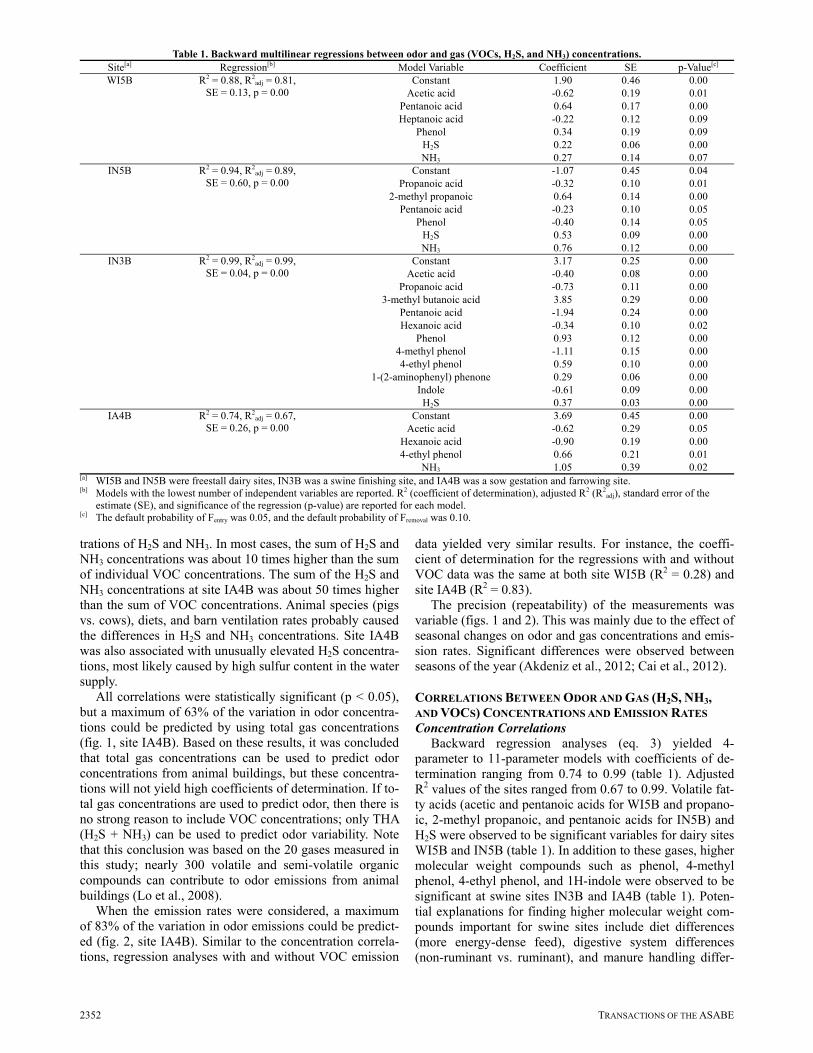
Backward regression analyses (eq. 3) yielded 4-parameter to 11-parameter models with coefficients of de-termination ranging from 0.74 to 0.99 (table 1). Adjusted R2 values of the sites ranged from 0.67 to 0.99. Volatile fat-ty acids (acetic and pentanoic acids for WI5B and propano-ic, 2-methyl propanoic, and pentanoic acids for IN5B) and H2S were observed to be significant variables for dairy sites WI5B and IN5B (table 1). In addition to these gases, higher molecular weight compounds such as phenol, 4-methyl phenol, 4-ethyl phenol, and 1H-indole were observed to be significant at swine sites IN3B and IA4B (table 1). Poten-tial explanations for finding higher molecular weight com-pounds important for swine sites include diet differences (more energy-dense feed), digestive system differences (non-ruminant vs. ruminant), and manure handling differ-

Table 1. Backward multilinear regressions between odor and gas (VOCs, H2S, and NH3) concentrations. Site[a] Regression[b] Model Variable Coefficient SE p-Value[c] WI5B R2 = 0.88, R2

adj = 0.81, SE = 0.13, p = 0.00

Constant 1.90 0.46 0.00 Acetic acid -0.62 0.19 0.01

Pentanoic acid 0.64 0.17 0.00 Heptanoic acid -0.22 0.12 0.09

Phenol 0.34 0.19 0.09 H2S 0.22 0.06 0.00 NH3 0.27 0.14 0.07

IN5B R2 = 0.94, R2adj = 0.89,

SE = 0.60, p = 0.00 Constant -1.07 0.45 0.04

Propanoic acid -0.32 0.10 0.01 2-methyl propanoic 0.64 0.14 0.00

Pentanoic acid -0.23 0.10 0.05 Phenol -0.40 0.14 0.05

H2S 0.53 0.09 0.00 NH3 0.76 0.12 0.00

IN3B R2 = 0.99, R2adj = 0.99,

SE = 0.04, p = 0.00 Constant 3.17 0.25 0.00

Acetic acid -0.40 0.08 0.00 Propanoic acid -0.73 0.11 0.00

3-methyl butanoic acid 3.85 0.29 0.00 Pentanoic acid -1.94 0.24 0.00 Hexanoic acid -0.34 0.10 0.02

Phenol 0.93 0.12 0.00 4-methyl phenol -1.11 0.15 0.00 4-ethyl phenol 0.59 0.10 0.00

1-(2-aminophenyl) phenone 0.29 0.06 0.00 Indole -0.61 0.09 0.00 H2S 0.37 0.03 0.00

IA4B R2 = 0.74, R2adj = 0.67,

SE = 0.26, p = 0.00 Constant 3.69 0.45 0.00

Acetic acid -0.62 0.29 0.05 Hexanoic acid -0.90 0.19 0.00 4-ethyl phenol 0.66 0.21 0.01

NH3 1.05 0.39 0.02 [a] WI5B and IN5B were freestall dairy sites, IN3B was a swine finishing site, and IA4B was a sow gestation and farrowing site. [b] Models with the lowest number of independent variables are reported. R2 (coefficient of determination), adjusted R2 (R2

adj), standard error of the estimate (SE), and significance of the regression (p-value) are reported for each model.

[c] The default probability of Fentry was 0.05, and the default probability of Fremoval was 0.10.

55(6): 2347-2356 2353

ences (long-term manure underfloor storage of swine ma-nure vs. flushing of dairy manure to outside storage basins).

Stepwise regression analyses yielded lower coefficients of determination (0.53 to 0.69) than the backward method, but fewer variables were included in the stepwise models (table 2). While odor was comprised of several compounds, the most significant were pentanoic acid and H2S (R2 = 0.69) at dairy site WI5B, 2-methyl propanoic acid (R2 = 0.58) at dairy site IN5B, H2S (R2 = 0.53) at swine finishing site IN3B, and NH3 and 4-ethyl phenol at sow site IA4B. These particular compounds apparently can be used to ac-count for up to 69% of the variance in odor concentrations.

The models developed with the stepwise method were cross-validated by splitting the data into a training data set (randomly selected data points that account for 60% of the data) and a testing data set (the remaining data). Average R2 values of the training data set were close to the R2 values of the developed models, which indicated that the models were valid (table 2).

The most significant compounds were found to be dif-ferent for each site. This was expected, since odor and gas concentrations and emission rates were significantly differ-ent due to variations in the barn and management character-istics of the sites. Both WI5B and IN5B had freestall dairy

Table 2. Stepwise multilinear regressions between odor and gas (VOCs, H2S, and NH3) concentrations. Sites[a] Model Regression[b] Model Variables Coefficient SE p-Value[c] WI5B 1 R2 = 0.61, R2

adj = 0.6, SR = 0.19, p = 0.00,

R2training = 0.60

Constant 2.48 0.06 0.00 Pentanoic acid 0.23 0.05 0.00

2 R2 = 0.69, R2adj = 0.66,

SE = 0.19, p = 0.00, R2

training = 0.65

Constant 2.25 0.12 0.00 Pentanoic acid 0.18 0.05 0.00

H2S 0.12 0.06 0.04 IN5B 1 R2 = 0.59, R2

adj = 0.55, SE = 0.13, p = 0.00,

R2training = 0.52

Constant 2.21 0.04 0.00 2-methyl propanoic acid 0.33 0.08 0.00

IN3B 1 R2 = 0.53, R2adj = 0.51,

SE = 0.27, p = 0.00, R2

training = 0.49

Constant 1.94 0.23 0.00 H2S 0.39 0.09 0.00

IA4B 1 R2 = 0.56, R2adj = 0.54,

SE = 0.31, p = 0.00, R2

training = 0.51

Constant -1.56 1.03 0.15 NH3 1.30 0.28 0.00

2 R2 = 0.68, R2adj = 0.64,

SE = 0.27, p = 0.00, R2

training = 0.62

Constant -1.07 0.93 0.27 NH3 1.05 0.27 0.00

4-ethyl phenol -0.73 0.30 0.03 [a] WI5B and IN5B were freestall dairy sites, IN3B was a swine finishing site, and IA4B was a sow gestation/farrowing site. Two models were found

for the WI5B and IA4B sites, and one model was found for the IN5B and IN3B sites. [b] The validity of the models developed with the stepwise method was tested (cross-validated) by splitting the data into a training data set (randomly

selected data points that accounted for 60% of the data) and a testing data set (the rest of the data). Random data selection was repeated three times, and an average R2 value was calculated for the training data set (R2

training). [c] The default probability of Fentry was 0.05, and the default probability of Fremoval was 0.10.

Table 3. Backward multilinear regressions between odor and gas (VOCs, H2S, and NH3) emission rates.

Site[a] Regression[b] Model Variables Coefficient SE p-Value[c] WI5B R2 = 0.99, R2

adj = 0.97, SE = 0.09, p = 0.00

Constant 3.20 0.27 0.00 Acetic acid -1.16 0.16 0.00 Butyric acid 0.88 0.18 0.00

3-methyl butanoic acid -1.49 0.37 0.01 Pentanoic acid 1.49 0.21 0.00 Hexanoic acid 1.71 0.24 0.00

Phenol -0.75 0.13 0.00 4-methyl phenol -0.33 0.08 0.01

IN5B R2 = 0.97, R2adj = 0.95,

SE = 0.11, p = 0.00 Constant 6.72 0.39 0.00

2-methyl propanoic acid 0.80 0.13 0.00 3-methyl butanoic acid -3.03 0.34 0.00

Pentanoic acid 1.26 0.23 0.01 IN3B R2 = 0.57, R2

adj = 0.48, SE = 0.39, p = 0.02

Constant 1.21 0.79 0.16 Propanoic acid 2.11 0.66 0.01

3-methyl butanoic acid -1.89 0.73 0.03 IA4B R2 = 0.77, R2

adj = 0.64, SE = 0.21, p = 0.00

Constant 2.39 1.11 0.05 Propanoic acid 0.92 0.35 0.02

3-methyl butanoic acid -1.52 0.52 0.01 Pentanoic acid 0.91 0.47 0.08 Hexanoic acid -0.79 0.27 0.01

4-methyl phenol 1.63 0.60 0.02 4-ethyl phenol -1.79 0.48 0.00

3-methyl-1H-indole 0.54 0.10 0.00 [a] WI5B and IN5B were freestall dairy sites, IN3B was a swine finishing site, and IA4B was a sow gestation/farrowing site. [b] Models with the lowest number of independent variables are reported. R2 (coefficient of determination), adjusted R2 (R2

adj), standard error of the estimate (SE), and significance of the regression (p-value) are reported for each model.

[c] The default probability of Fentry was 0.05, and the default probability of Fremoval was 0.10.

2354 TRANSACTIONS OF THE ASABE

barns, but the ventilation systems, manure collection meth-ods, bedding types, and animal weights were different be-tween the sites (Akdeniz et al., 2012). Many studies have demonstrated that diet has significant effects on odor emis-sions from swine manure (Willing et al., 2005; Le et al., 2005; Le et al., 2008).

Dimethyl disulfide and dimethyl trisulfide are known to be odorous compounds with relatively low odor detection thresholds (Parker et al., 2010). Surprisingly, dimethyl di-sulfide, diethyl disulfide, and dimethyl trisulfide were not significant for any of the sites. This might have been due to the low sample sizes for these compounds, since they were only analyzed during the last few months of the project. This should be further investigated in future studies.

Emission Rate Correlations Backward and stepwise correlations between odor and

gas emission rates are given in tables 3 and 4, respectively (eq. 4). When the backward method was used, high coeffi-cients of determination (ranging from 0.57 to 0.98) were observed for all sites. The highest coefficients were for pentanoic and hexanoic acids at site WI5B, 3-methyl buta-noic and pentanoic acids at site IN5B, propanoic acid at site IN3B, and propanoic acid, 4-methyl phenol, and 3-methyl-1H indole at site IA4B. With the stepwise method, pentano-ic and hexanoic acids were observed to be the most signifi-cant compounds for site WI5B (table 4). The most signifi-cant compound for site IA4B was 3-methyl-1H-indole, but the coefficient of the model was low (0.32) (table 4). No linear correlations were observed for sites IN5B and IN3B.

Based on these results, it was concluded that gas concentra-tions rather than emission rates should be used to predict odor emissions variability. In future studies, polynomial re-gression models can be tested to find better correlations be-tween odor and gas emission rates of livestock buildings.

CORRELATIONS BETWEEN ODOR AND GAS (H2S AND NH3) CONCENTRATIONS AND EMISSION RATES

When VOCs were excluded from the model and correla-tions between concentrations of odor and H2S and NH3 gases (eq. 5) were investigated, significant correlations (R2 ranged from 0.42 to 0.83) were observed (table 5). For sites WI5B and IN3B, only H2S was observed to be significant, while for sites IN5B and IA4B both H2S and NH3 were ob-served to be significant (p < 0.05). Although H2S and NH3 correlations had lower R2 values than the values observed with 20 gases (H2S, NH3, and VOCs), they can be used to estimate variability in odor concentrations when VOC data are not available. Noble et al. (2001) and Blanes-Vidal et al. (2009) also reported good correlations between odor and H2S concentrations. Noble et al. (2001) reported high corre-lations between odor and H2S concentrations for mushroom composting sites, but they observed poor correlations be-tween odor and NH3 concentrations. Blanes-Vidal et al. (2009) observed that H2S accounted for 68% of the varia-tion in odor concentrations above the stirred slurry samples. It was reported that the contribution of ammonia to the odor concentrations was only significant in the absence of H2S. When correlations between odor and H2S and NH3 emis-sion rates (eq. 6) were evaluated, both H2S and NH3 were

Table 4. Stepwise multilinear regressions between odor and gas (VOCs, H2S, and NH3) emission rates. Sites[a] Model Regression[b] Model Variables Coefficient SE p-Value[c] WI5B 1 R2 = 0.69, R2

adj = 0.67, SE = 0.28, p = 0.00,

R2training = 0.60

Constant 2.86 0.27 0.00 Pentanoic acid 0.62 0.12 0.00

2 R2 = 0.79, R2adj = 0.76,

SE = 0.24, p = 0.00, R2

training = 0.70

Constant 2.96 0.23 0.00 Pentanoic acid 1.60 0.44 0.00 Hexanoic acid -1.08 0.47 0.04

IA4B 1 R2 = 0.32, R2adj = 0.29,

SE = 0.29, p = 0.00, R2

training = 0.25

Constant 4.52 0.11 0.00 3-methyl-1H-indole 0.22 0.08 0.01

[a] WI5B and IN5B were freestall dairy sites, IN3B was a swine finishing site, and IA4B was a sow gestation/farrowing site. No linear regression was found for the IN5B and IN3B sites. Two models were found for the WI5B site, and one model was found for the IA4B site.

[b] The validity of the models developed with the stepwise method was tested (cross-validated) by splitting the data into a training data set (randomly selected data points that accounted for 60% of the data) and a testing data set (the rest of the data). Random data selection was repeated three times, and an average R2 value was calculated for the training data set (R2

training). [c] The default probability of Fentry was 0.05, and the default probability of Fremoval was 0.10.

Table 5. Multilinear regressions between odor and gas (H2S and NH3) concentrations (enter method). Sites[a] Regression[b] Model Variables Coefficient SE p-Value WI5B R2 = 0.43, R2

adj = 0.38, SE = 0.32, p = 0.00

Constant 1.98 0.39 0.00 H2S 0.30 0.07 0.00 NH3 -0.44 0.14 0.75

IN5B R2 = 0.69, R2adj = 0.64,

SE = 0.11, p = 0.00 Constant 0.38 0.34 0.29

H2S 0.21 0.06 0.00NH3 0.42 0.09 0.00

IN3B R2 = 0.83, R2adj = 0.79,

SE = 0.19, p = 0.00 Constant 1.78 0.29 0.00

H2S 0.61 0.14 0.00 NH3 -0.13 0.14 0.38

IA4B R2 = 0.63, R2adj = 0.62,

SE = 0.46, p = 0.00 Constant -0.27 0.45 0.54

H2S 0.10 0.22 0.04 NH3 0.84 0.28 0.00

[a] WI5B and IN5B were freestall dairy sites, IN3B was a swine finishing site, and IA4B was a sow gestation and farrowing site. [b] R2 (coefficient of determination), adjusted R2 (R2

adj), standard error of the estimate (SE), and significance of the regression (p-value) are reported for each model. Significant p-values are in boldface type.

55(6): 2347-2356 2355

found to be significant for site WI5B, while only H2S was significant for sites IN5B and IN3B (table 6). For site IA4B, although the overall coefficient of determination was found to be significant (R2 = 0.25, p = 0.04), only the con-stant value was significant, and none of the gases (H2S and NH3) had significant coefficients (table 6). Similar to the results of the regression analysis between odor and 20 gas-es (VOC, H2S, and NH3), concentrations of H2S and NH3, rather than emission rates, can be used to estimate odor var-iability.

CONCLUSIONS The following conclusions were drawn from this re-

search: Summed concentrations of gases can be used to predict

up to 63% of the variation in odor samples. If summed con-centrations are used to predict odor, there is no strong rea-son to include VOC concentrations since there was slight difference between the correlations observed for THAV (H2S + NH3 + VOCs) and the correlations observed for THA (H2S + NH3).

When gas concentrations were assessed, H2S, NH3, ace-tic acid, propanoic acid, 2-methyl propanoic acid, pentanoic acid, and phenol were observed to be significant gases for the dairy sites. For the swine sites, in addition to some of these gases, higher molecular weight compounds such as 4-methyl phenol, 4-ethyl phenol, and 1H-indole were also found to be significant.

When the emission rates of the gases were taken into ac-count, the most significant compounds were pentanoic and hexanoic acids for site WI5B, pentanoic acid for site IN5B, propanoic acid for site IN3B, and propanoic acid, 4-methyl phenol (p-cresol) and 3-methyl-1H indole (skatole) for site IA4B.

When VOCs were excluded from the model, significant correlations were still observed between odor and H2S and NH3 concentrations. Although these coefficients were less significant than observed for 20 gases (VOCs, H2S, and NH3), they can be used to predict odor variability when VOC data are not available. In many cases, VOC data are unavailable since their measurement requires advanced analytical techniques, while H2S and NH3 can be easily measured with continuous gas analyzers.

This article highlights the most significant contributors to odor production inside animal buildings. To test the ap-plicability of the models to other geographic locations and livestock barns, future studies should collect additional samples from different types of animals and sites. In addi-tion, developing separate regression equations for cool and warm seasons may help to find higher linear correlations between odor and gas concentrations and emission rates.

ACKNOWLEDGEMENTS This project was supported by National Research Initia-

tive Competitive Grant No. 2005-35112-15336 from the USDA Cooperative State Research, Education, and Exten-sion Service Air Quality Program. The authors gratefully acknowledge Blanca Martinez, Erin L. Cortus, Teng T. Lim, Katie T. Heathcote, Steven J. Hoff, and Edward A. Caraway for their contributions during sample collection and analysis.

REFERENCES Akdeniz, N., L. D. Jacobson, B. P. Hetchler, S. D. Bereznicki, A.

J. Heber, J. A. Koziel, L. Cai, S. Zhang, and D. B. Parker. 2012a. Odor and odorous chemical emissions from animal buildings: Part 2. Odor emissions. Trans. ASABE 55(6): 2335-2345.

Bereznicki, S. D., A. J. Heber, N. Akdeniz, L. D. Jacobson, B. P. Hetchler, K. Y. Heathcote, S. J. Hoff, J. A. Koziel, L. Cai, S. Zhang, D. B. Parker, E. A. Caraway, T. T. Lim, E. L. Cortus, and R. B. Jacko. 2012. Odor and odorous chemical emissions from animal buildings: Part 1. Project overview, collection methods, and quality control. Trans. ASABE 55(6): 2325-2334.

Blanes-Vidal, V., M. N. Hansen, A. P. S. Adamsen, A. Feilberg, S. O. Peterson, and B. B. Jensen. 2009. Characterization of odor released during handling of swine slurry: Part I. Relationship between odorants and perceived odor concentrations. Atmos. Environ. 43(18): 2997-3005.

Cai, L., J. A. Koziel, S. Zhang, E. L. Cortus, D. B. Parker, S. J. Hoff, G. Sun, K. Y. Heathcote, L. D. Jacobson, N. Akdeniz, B. P. Hetchler, S. D. Bereznicki, A. J. Heber, E. A. Caraway, and T. T. Lim. 2012. Odor and odorous chemical emissions from animal buildings: Part 3. Chemical emissions. Trans. ASABE (in review).

Gostelow, P., and S. A. Parsons. 2000. Sewage treatment works odour measurement. Water Sci. Tech. 41(6): 33-40.

Guo, H., W. Dehod, J. Agnew, C. Lague, J. R. Feddes, and S. Pang. 2006. Annual odor emission rate from different types of

Table 6. Multilinear regressions between odor and gas (H2S and NH3) emission rates (enter method). Sites[a] Regression[b] Model Variables Coefficients SE p-Value WI5B R2 = 0.43, R2

adj = 0.37, SE = 0.42, p = 0.00

Constant -2.94 2.83 0.31 H2S 0.37 0.11 0.00NH3 1.15 1.15 0.04

IN5B R2 = 0.97, R2adj = 0.94

SE = 0.03, p = 0.03 Constant 3.69 0.48 0.02

H2S 0.32 0.04 0.02 NH3 -0.06 0.09 0.55

IN3B R2 = 0.69, R2adj = 0.59,

SE = 0.39, p = 0.03 Constant -0.25 1.97 0.91

H2S 0.89 0.27 0.02NH3 0.14 0.42 0.76

IA4B R2 = 0.25, R2adj = 0.18,

SE = 0.33, p = 0.04 Constant 2.38 0.91 0.02

H2S 0.11 0.39 0.78 NH3 0.36 0.39 0.36

[a] WI5B and IN5B were freestall dairies, IN3B was a swine finishing site, and IA4B was sow gestation and farrowing site. [b] R2 (coefficient of determination), adjusted R2 (R2

adj), standard error of the estimate (SE), and significance of the regression (p-value) are reported for each model. Significant p-values are in boldface type.

2356 TRANSACTIONS OF THE ASABE

swine production buildings. Trans ASABE 49(2): 517-525. Guo, H., W. Dehod, J. Agnew, J. R. Feddes, C. Lague, and S.

Pang. 2007. Daytime odor emission variations from various swine barns. Trans. ASABE 50(4): 1365-1372.

Heber, A. J., B. W. Bogan, J.-Q. Ni, T. T. Lim, E. L. Cortus, J. C. Ramirez-Dorronsoro, C. A. Diehl, S. M. Hanni, C. Xiao, K. D. Casey, C. A. Gooch, L. D. Jacobson, J. A. Koziel, F. M. Mitloehner, P. M. Ndegwa, W. P. Robarge, L. Wang, and R. Zhang. 2008. The National Air Emissions Monitoring Study: Overview of barn sources. Paper presented at the 8th International Livestock Environment Symposium. ASABE Publication No. 701P0408. St. Joseph, Mich.: ASABE.

Jacobson, L. D., C. J. Clanton, D. R. Schmidt, C. Radman, R. E. Nicolai, and K. A. Janni. 1997. Comparison of hydrogen sulfide and odor emissions from animal manure storages. In Proc. Intl. Symp. on Ammonia and Odour Control from Animal Production Facilities, 405. J. A. M. Voermans and G. Monteny, eds. Vinkeloord, The Netherlands: CIGR.

Jacobson, L. D., H. Guo, D. R. Schmidt, R. E. Nicolai, J. Zhu, and K. A. Janni. 2005. Development of the OFFSET model for determination of odor-annoyance-free setback distances from animal production sites: Part I. Review and experiment. Trans. ASAE 48(6): 2259-2268.

Jacobson, L. D., B. P. Hetchler, D. R. Schmidt, R. E. Nicolai, A. J. Heber, J.-Q. Ni, S. J. Hoff, J. A. Koziel, D. B. Parker, Y. Zhang, and D. B. Beasley. 2008. Quality assured measurements of animal building emissions: Part 3. Odor concentrations. J. Air and Waste Mgmt. Assoc. 58(6): 806-811.

Jacobson, L. D., N. Akdeniz, L. Cai, S. Zhang, J. A. Koziel, S. A. Hoff, K. Heathcote, A. J. Heber, S. D. Bereznicki, D. B. Parker, and E. A. Caraway. 2010. Odor emissions and chemical analysis of odorous compounds from animal buildings. In Proc. WEF Conf.: Odors and Air Pollutants, 864-885. Washington, D.C.: Water Environment Federation.

Jin, Y., T. T. Lim, J.-Q. Ni, J.-H. Ha, and A. J. Heber. 2012. Emissions monitoring at a deep-pit swine finishing facility: Research methods and system performance. J. Air and Waste Mgmt. Assoc. (in press, doi: 10.1080/10962247.2012.707163).

Le, P. D., A. J. A. Aarnink, N. W. M. Ogink, P. M. Becker, and M. W. A. Verstegen. 2005. Odor from animal production facilities: Its relationship to diet. Nutrition Res. Rev. 18(1): 3-30.

Le, P. D., A. J. A. Aarnink, A. W. Jongbloed, C. M. C. van de Peet-Schwering, M. W. A. Verstegen, and N. W. M. Ogink. 2008. Interactive effects of dietary crude protein and fermentable carbohydrate levels on odor from pig manure. Livestock Sci. 114(1): 48-61.

Lo, Y. C., J. A., Koziel, L. Cai, S. J. Hoff, W. S. Jenks, and H. Xin. 2008. Simultaneous chemical and sensory characterization of VOCs and semi-VOCs emitted from swine

manure using SPME and multidimensional gas chromatography-mass spectrometry-olfactometry system. J. Environ. Qual. 37(2): 521.

Ni, J.-Q., A. J. Heber, M. J. Darr, T. T. Lim, C. A. Diehl, and B. W. Bogan. 2009. Air quality monitoring and on-site computer system for livestock and poultry environment studies. Trans. ASABE 52(3): 937-947.

Noble, R., P. J. Hobbs, A. Dobrovin-Pennington, T. H. Misselbrook, and A. Mead. 2001. Olfactory response to mushroom composting emissions as a function of chemical concentration. J. Environ. Qual. 30(3): 760-767.

NRC. 2003. The scientific basis for estimating emissions from animal feeding operations. Washington, D.C.: National Research Council.

Parker, D. P. 2008. Reduction of odor and VOC emissions from a dairy lagoon. Applied Eng. in Agric. 24(5): 647-655.

Parker, D. B., Z. L. Perschbacher-Buser, N. A. Cole, and J. A. Koziel. 2010. Recovery of agricultural odors and odorous compounds from polyvinyl fluoride film bags. Sensors 10(9): 8536-8552.

Parker, D. B., J. A. Koziel, L. Cai, L. D. Jacobson, N. Akdeniz, S. D. Bereznicki, T. T. Lim, E. A. Caraway, S. Zhang, S. J. Hoff, A. J. Heber, K. Y. Heathcote, and B. P. Hetchler. 2012. Odor and odorous chemical emissions from animal buildings: Part 6. Odor activity value. Trans. ASABE 55(6): 2357-2368.

Qu, G., I. E. Edeogu, and J. J. R. Feddes. 2010. Odor index: An integration of odor parameters for swine slurry odors. Trans. ASABE 53(1): 219-223.

SPSS. 2008. Statistics 17.0.1 User’s Guide. Chicago, Ill.: SPSS, Inc.

Willing, S., D. Losel, and R. Claus. 2005. Effects of resistant potato starch on odor emission from feces in swine production units. J. Agric. Food Chem. 53(4): 1173-1178.

Zahn, J. A. J. L. Hatfield, Y. S. Do, A. A. Dispirito, D. A. Laird, and R. L. Pfeiffer. 1997. Characterization of volatile organic emissions and wastes from a swine production facility. J. Environ. Qual. 26(6): 1687.

Zhang, S., L. Cai, J. A. Koziel, S. J. Hoff, D. R. Schmidt, C. J. Clanton, L. D. Jacobson, D. P. Parker, and A. J. Heber. 2010. Field air sampling and simultaneous chemical and sensory analysis of livestock odorants with sorbent tubes and GC-MS/olfactometry. Sensors and Actuators B 146(2): 427-432.

Zhang, S., L. Cai, J. A. Koziel, S. J. Hoff, K. Y. Heathcote, L. Chen, L. D. Jacobson, N. Akdeniz, B. P. Hetchler, D. B. Parker, E. A. Caraway, A. J. Heber, and S. D. Bereznicki. 2012. Odor and odorous chemical emissions from animal buildings: Part 5. Correlations between odor intensities and chemical concentrations (GC-MS-O). Trans. ASABE (in review).