Embed Size (px)
Citation preview

Part 1
• Course administration
• Overview of course syllabus
• An example of a real-life auction: The sale of Bezeq.
• Definitions: normal-form games, dominant strategies, Nash equilibrium.
• One-item auctions: analysis of the 2nd price auction.

Course administration
• Grade is based on two components of equal weight:
– Giving a 20-minutes talk. This assignment can be done in couples (10 minutes each).
AND
– Multiple choice exam (15 questions, 1.5 hours)
OR solving a final exercise at home. The exercise contains difficult mathematical questions, and is intended only for students who want a mathematical challenge.
• Course website on moodle. All material is there.

Presentations• Possible topics for presentations are detailed in moodle.
– Book chapters, research papers, webpages on research
– Main focus should be the connection of theory to practice, so maybe add real-life examples that you search over the Internet searches.
• Email me which chapter would you like to do. I will update in the moodle site with the already occupied subjects and slots.
• Each week, three people will give a talk (a group of two can be split between two consecutive weeks).
• Next week the presentations should be about “stable matching”. I will give a 15-points bonus for this topic. The first three to email will have the slots.

What is Auction Theory?• Auctions are becoming more and more popular
– The Internet only helps.
• We see different auction formats, different rules.
– Can we say anything about the difference, what will be the result of one format vs. another.
– Examples: Ebay has proxies, different sites has different end rules, etc.
• How to analyze this? We use Game Theory, that models strategic decisions of players.
• The course will describe the mathematical theory that evolved (but with very little mathematical proofs)

הסיפור מאחורי הפרטת בזק
2005 למאי 29מקור: "הארץ", •
שתי קבוצות התמודדו במכרז: קבוצת סבן, וקבוצת אלג'ם.•
מיליארד3.6 מיליארד , סבן: 3.2ההצעות ההתחלתיות - אלג'ם: •
התכנון המקורי של משרד האוצר היה לחשוף את ההצעות, ולקבל הצעות •חדשות (כלומר לערוך מכרז אנגלי עולה). אבל לנוכח הפער הגדול בין שתי
מיליון שקל), באוצר חששו להמשיך לפי התכנון המקורי, 400ההצעות (שמא אלג'ם תתייאש ותפרוש.
היועץ המקצועי, פרופ' מוטי פרי מירושלים, התעקש להמשיך לפי התכנון: •"אין ביטחון מלא, אבל בדרך כלל השקיפות מביאה לתוצאות הטובות
ביותר. יש למסור לכל אחד מהמשתתפים את תוצאות הסבב הראשון... ההצעה העיקרית שלי במכרז היתה ליצור מערכת שקופה לחלוטין, שבה כל אחד מהצדדים יודע בדיוק מה קורה ומקבל את כל המידע. ככל שלמתחרים
יש יותר ידע, רמת הסיכון שלהם יורדת, מרכיב ההימור בעסקה יורד, והם מוכנים להסתכן בהצעות גבוהות יותר".

הסיפור מאחורי הפרטת בזק
מיליארד.3.6 מיליארד , סבן: 3.2ההצעות ההתחלתיות - אלג'ם: •
מיליארד, 4.11 מיליארד, וסבן העלה ל-3.8המשך המכרז: אלג'ם העלו ל-•וניצח.
מכרז בזק היה המכרז הראשון בתולדות ההפרטה שנוהל על פי ייעוץ של •פרופ'
לתורת המשחקים. תוצאות המכרז הוכיחו שגישה זו הייתה נכונה.

Course Overview
1. Basic game-theoretic notions, The basic auction model, description and analysis of classic one-item auctions.
2. Revenue-maximizing auctions for one item.
3. Bidders with interdependent values.
4. Mechanism Design and VCG.
5. Auctions for multiple goods.

Four “classic” auctions
• First price: bidders submit bids. Winner is the highest bidder. Pays her bid.
• Second price: bidders submit bids. Winner is the highest bidder. Pays her bid.
• Dutch auction: price starts from a very high number, and gradually descends. First one to raise her hand wins. Pays that price.
• English auction: price starts from zero, and gradually ascends. Last one to keep her hand up wins. Pays that price.

Simulation• Each student gets a different amount of virtual dollars: two last
digits of ID number.
• I will conduct two auctions:submit a note that contains your name and ID number, and your bid for the first and second price auctions.
• Each winner pays the price she owes me with her virtual dollars. Each remaining virtual dollar will give one bonus point in the final grade (and vice versa - if she cannot pay the entire price with her virtual dollars, I will deduct the difference from the grade!).

A game (in complete information)
Action “T”
Action “B”
Action “R”Action “L”
Player I’s actions
Player II’s actions
Here’re the utilities if player I plays T and II plays L
5 , -3
If player I plays B and II plays R then player I gets 5 and II gets -3

Example: Prisoner’s dilemma
• The story: Business partners decide to break down, and each one needs to hire a lawyer, to reach a settlement on how to split their property. Total property is worth 10.– Two types of lawyers: cheap costs 1, expensive costs 5.– If both choose same type, property is split equally.– Otherwise the one with the expensive lawyer gets everything.
• So, the game is:
“C”
“E” 0 , 0
“C” “E”
4 , 4
5 , -1
-1 , 5

What will happen in this game?
DFN: Action A dominates action B (for player i) if for any combination of actions of the other players, a-i, ui(A,a-i) > ui(B,a-i).Action A is a dominant action if it dominates all other actions.
• Observation:“E” is a dominant strategy.
• Assumption: Players indeedplay a dominant strategy ifthey have one.
• Demonstration:the reality show
“C”
“E” 0 , 0
“C” “E”
4 , 4
5 , -1
-1 , 5

A one-item auctionThe story:
• A seller wishes to sell a good to n players. Player i will obtain a value of vi > 0 from having the good. vi is known only to i.
• The seller can charge a payment pi from player i.In this case player i’s utility is: vi – pi
• Like we did in the beginning of the class.

Analysis of second price
• Example: three players. v1 = 10, v2 = 7, v3 = 4.
• If they all bid their true values, player 1 wins, and pays 7.
• Notice that none of the players can improve her utility by changing her bid.
THM: In the second price auction, bidding the true value is a dominant strategy.

Drawing the game (for two players)
• The strategy space of each player is composed of all integers.
• For fixed v1, v2, if player 1 plays b1 and player 2 plays b2,and b2 > b1, then the utility of player 1 is 0, and of 2 is v2 – b1.
.
.
.b1
b2
0, v2 – b1

Analysis for n=2Claim: A dominant action for player i=1,2 is to play bi=vi
Proof: Fix any b2
• If v1 > b2 then winning is better than losing for player 1. Declaring b1=v1 will cause player 1 to win.
• If v1 < b2 then losing is better than winning for player 1. Declaring b1=v1 will cause player 1 to lose.
• Conclusion: no matter what the other player declared, the strategy b1=v1 dominates all other strategies of player 1.

Analysis for n>2
• For n > 2 players the game and the claim are similar.
Claim: The dominant action of player i is to play bi=vi
Proof: Fix any b-i , and let x = max j i bj
• If vi > x then winning is better than losing for player i. Declaring bi=vi will cause player i to win.
• If vi < x then losing is better than winning for player i. Declaring bi=vi will cause player i to lose.

Equivalence of second price and English auctions
• In the English auction, the dominant strategy of every player is to drop exactly when the price reaches her value.
• If all players do that, then the player with the highest value wins, and she pays the second highest value (since the price stops exactly when the second highest player drops).

Next: 1st price auction
• What about the 1st price rule?
• If players continue to bid their true value, then this auction will clearly have a higher revenue.
• But of-course players adjust their behavior according to the rules of the auction.
• Observation: There is no dominant strategy in the 1st price auction (if a player wins with a bid b he would have preferred to say slightly less than b).

Part 2
• We started by talking about the four classic auctions, and about analyzing them using game theory.
• We continue by reviewing the theoretical analysis of these auctions:
– Analyze the equilibrium strategies of these auctions.
– Describe another auction with a better revenue.
– Talk about two insightful lemmas, that are related to the construction of the auction.

Nash Equilibrium
• In the “coordination game”, players gain a positive utility if and only if they play the same action.
DFN
• Action ai is best response to a-i iffor any other action a’i of player i,ui(ai, a-i) > ui(a’i, a-i)
• The actions (a1,…,an) are in Nash equilibrium ai is best response to a-i for all players i.
• What are the Nash equilibria in the coordination game?
1 , 2
2 , 1
0 , 0
0 , 0“A”
“B”
“A” “B”

Example: the Braess paradox
• Using Nash Equilibrium to study transportation networks.
• The picture shows a road network. All cars need to arrive from node S to node T.
• There are two types of roads:
– label “1”: wide and long road, travel time is one hour regardless of number of cars.
– label “x”: narrow and short road, x is the fraction of cars that take this road, travel time is x times one hour. For exampleif ½ of all cars take this road then travel time is half an hour.
S T
x
x
1
1

Example: the Braess paradox
• If all cars take the upper path, total travel time will be 2.
• Drivers care only about their total travel time, which is influenced by the choices of all other drivers. Thus this is a game.
• What is a Nash equilibrium of this game?
S T
x
x
1
1
100%

Example: the Braess paradox
• If all cars take the upper path, total travel time will be 2.
• Drivers care only about their total travel time, which is influenced by the choices of all other drivers. Thus this is a game.
• What is a Nash equilibrium of this game?Answer: 50% of the drivers take each path. Total driving time of each driver is 1.5 hours.Remark: This is the unique Nash equilibrium.
S T
x
x
1
1
50%
50%

Example: the Braess paradox
S T
x
x
1
1
0
• Now the government has decided to expand the network and build a new fast road. What will happen?
• In other words what will be the new Nash equilibrium, and what will be the travel times in this equilibrium?

Example: the Braess paradox
• Now the government has decided to expand the network and build a new fast road. What will happen?
• In other words what will be the new Nash equilibrium, and what will be the travel times in this equilibrium?Answer: As in the picture. This is again the unique Nash equilibrium. Why?
S T
x
x
1
1
0100%

Example: the Braess paradox
• Now the government has decided to expand the network and build a new fast road. What will happen?
• In other words what will be the new Nash equilibrium, and what will be the travel times in this equilibrium?Answer: As in the picture. This is again the unique Nash equilibrium.
• Driving time of each driver is 2 hours, worse than before.
• The paradox: instead of helping, the government only made things worse. The lesson: strategic behavior can cause unexpected phenomena, and must be taken into account.
S T
x
x
1
1
0100%

Example: the Braess paradox• This has happened in reality:
• In NYC, the 42nd street was closed on Earth Day in 1990. Lucius J. Riccio, the transportation ommissioner at the time, said that “many predicted it would be doomsday“. However, to everyone’s surprise, traffic flow improved when the street closed.
• In Seoul, South Korea, traffic improved when a motorway was removed as part of the Cheonggyecheon restoration project -- an elevated highway was removed to uncover a historic waterway.
• In Stuttgart, Germany, initial investments into the road network in 1969 did not improve traffic. However, once a section of this newly-built road was closed, the traffic situation improved.
• In 2008, an academic research specified roads that, if closed, will reduce travel time in NYC, Boston, and London.

Back to auctions

Reminder: Four “classic” auctions
• First price: bidders submit bids. Winner is the highest bidder. Pays her bid.
• Second price: bidders submit bids. Winner is the highest bidder. Pays her bid.We saw that it is a dominant strategy to bid the true value.
• Dutch auction: price starts from a very high number, and gradually descends. First one to raise her hand wins. Pays that price.
• English auction: price starts from zero, and gradually ascends. Last one to keep her hand up wins. Pays that price.

Analysis of 1st price
• If players continue to bid their true value, then this auction will clearly have a higher revenue.
• But of-course players adjust their behavior according to the rules of the auction.
• Observation: There is no dominant strategy in the 1st price auction (if a player wins with a bid b he would have preferred to say slightly less than b). We will therefore use the notion of a Nash equilibrium.

Equilibrium in incomplete information
• Assumption: vi is drawn from a probability distribution fi, and these distributions are known to all (“common priors”).
• Useful example: vi is drawn from the uniform distribution on [0,1]. In this case:
– Pr(vi < 1/2) = 1/2. In general, for any 0 < x < 1, Pr(vi < x) = x.
– E[vi]=1/2.
• The strategies of the players are in (Bayesian-Nash) equilibriumif each player maximizes her expected profit by following her equilibrium strategy, given that the other players follow their strategies.

Equilibrium in the 1st price auction
THM: Assume each value is drawn from the uniform distribution on [0,1]. Then a Bayesian-Nash equilibrium of the 1st price auction is when every player i bids bi(vi) =[(n-1)/n] · vi
• Clearly, in the 1st price auction a bidder needs to “shade down” his value. This tells the players by how much.
– As the number of players grow, shading down becomes smaller.

Example
• n=2. Therefore, in equilibrium, every player bids half his value. Let’s see if this is indeed best for player 1, if his value is 2/3:
• u1(1/4) = (2/3 - 1/4) · Pr[ v2 / 2 < 1/4]
profit if wins probability to win

• n=2. Therefore, in equilibrium, every player bids half his value. Let’s see if this is indeed best for player 1, if his value is 2/3:
• u1(1/4) = (2/3 - 1/4) · Pr[ v2 / 2 < 1/4] = (5/12)(1/2) 0.208 Pr[ v2 < 1/2] = 1/2
Example

• n=2. Therefore, in equilibrium, every player bids half his value. Let’s see if this is indeed best for player 1, if his value is 2/3:
• u1(1/4) = (2/3 - 1/4) · Pr[ v2 / 2 < 1/4] = (5/12)(1/2) 0.208 Pr[ v2 < 1/2] = 1/2
• u1(1/3) = (2/3 - 1/3) · Pr[ v2 / 2 < 1/3] = (1/3)(2/3) 0.222 Pr[ v2 < 2/3] = 2/3
• u1(1/2) = (2/3 - 1/2) · Pr[ v2 / 2 < 1/2] = 1/6 0.167 Pr[ v2 < 1] = 1
Example

Remarks• 1st price auction is equivalent to a descending (“Dutch”) auction: the
auctioneer gradually lowers the price, the first to accept wins, for this price.
• A comparison to second price:
– No dominant strategies, so less obvious how to play.
– In both auctions, in equilibrium, the bidder with the highest value gets the item (the “efficient” outcome).
– 2nd price may look bad - the winner’s price may be much lower than his bid. An extreme once happened in a New-Zealand government-auction: One firm bid NZ$100,000 for a license, and paid the second-highest price of only NZ$6 (http://www.economicprincipals.com/issues/06.05.21.html).
– Compare these strategies to what you chose to do last class.

Revenue considerations
• Which of the two auctions raises more revenue?
• Is there an auction with a higher revenue than both these auctions?

Numerical example
VAL 1 VAL 2 1st price revenue 2nd price revenue optimal revenue96 64 48 64 6452 18 26 18 5036 78 39 36 5094 39 47 39 5058 23 29 23 5012 38 19 12 029 24 14.5 24 047 33 23.5 33 088 19 44 19 502 78 39 2 50
87 64 43.5 64 6496 84 48 84 8444 79 39.5 44 5011 27 13.5 11 038 72 36 38 505 82 41 5 50
52 46 26 46 5050 16 25 16 5051 14 25.5 14 50
33 31.15789 42.73684

• The symmetric case: players’ values are drawn from the same distribution, F(v). Choose v* that solves v = (1-F(v))/f(v).
• Then, English auction when the price starts from v* is the revenue maximizing auction:
– If the highest value is below v*, no one wins
– If the highest value is above v* and the second highest is below v*, the highest player wins and pays v*.
– If the second highest is above v*, the highest wins and pays the second highest.
The optimal auction for symmetric bidders

Numerical example
VAL 1 VAL 2 1st price revenue 2nd price revenue optimal revenue96 64 48 64 6452 18 26 18 5036 78 39 36 5094 39 47 39 5058 23 29 23 5012 38 19 12 029 24 14.5 24 047 33 23.5 33 088 19 44 19 502 78 39 2 50
87 64 43.5 64 6496 84 48 84 8444 79 39.5 44 5011 27 13.5 11 038 72 36 38 505 82 41 5 50
52 46 26 46 5050 16 25 16 5051 14 25.5 14 50
33 31.15789 42.73684

Practical Conclusion: Devote a large effort to figuring out the correct reservation price.

Remark
• How does such an auction increases the revenue of the regular English auction?
• The reservation price introduces two opposite effects:
– Sometimes the optimal auction does not sell the item, so the revenue is 0, while the English auction always sells the item (and thus always has a positive revenue).
– Sometimes the optimal auction sells the item but charges more than the second highest value, if it is below v*, while the price in the English auction is always the second highest value.
• The correct choice of v* enables the auctioneer to gain more from the second point and lose less from the first point.

Two observations that helped to find and prove this

The Revelation Principle
• Problem: there are infinitely many possible auction formats, so it is hard to go over all of them…
• Reminder: In a direct-revelation auction, the strategy space of a player is simply to report her type (value).
THM: Given any auction format with equilibrium strategies s(), there exists a direct-revelation auction for which truthfulness is an equilibrium, with the same outcome, and the same prices.
– Remark: This holds for any type of equilibrium (dominant strategies, Bayesian-Nash,...)
• The implication: we need only search for a direct-revelation auction.

Example
• We mimic the equilibrium strategy, hence truthfulness is an equilibrium.
• For example, suppose the true value of player 1 is 2/3.
– If she declares her true value it is as if she plays 1/3 in the 1st price auction.
– If she instead declares 1/2, it is as if she declares 1/4 in the 1st price auction. But we already know that this is not better in the 1st price auction.
1st price Auction
v1Convert to (1/2) v1
New Auction
Original Output
Input
v2Convert to (1/2) v2

Proof (sketch)
• A proxy mimics the equilibrium strategy: if others are truthful, player i would like to play si(vi), so she needs to declare vi.
• Examples:– In the 1st price auction, the proxy will convert vi to [(n-1)/n] vi
– In the English auction, the proxy will take vi and will keep “raising the hand” until the price reaches vi.
Original Auction“Proxy”
Input v Output s(v)
New Auction
Original Output

Conclusion: there is no revenue advantage for “complicated” indirect auctions (though there may
be a marketing advantage)

The Revenue Equivalence Theorem
THM (The Revenue Equivalence Theorem):
Suppose vi is drawn independently from some Fi(x). Take any two auctions such that, in both auctions:
- The expected utility of a player with value 0 is the 0.- The winner (in equilibrium) is always the same.
Then these two auctions raise the same expected revenue (in equilibrium) .
• The 1st and 2nd price auctions satisfy the conditions (in equilibrium, the item is sold to the bidder with the highest value), so they raise the same revenue. Another example: an all-pay auction. Here, too, the winner is the person with the highest value, so the revenue is the same.
• Why is the optimal auction different?

Conclusion: To design a revenue-maximizing auction, the only question is who will be the winner (in
equilibrium).

Risk aversion in 1st and 2nd price auctions
• A crucial assumption in the analysis of the 1st price auction is that players aim to maximize the expected profit.
– This is termed risk-neutral players.
– Many times this is not true: for example, we might care about the variance (smaller variance might be better).
• In a 2nd price auction, the dominant strategy is to bid truthfully, so risk-aversion does not change anything.
– There is no expectation in the considerations of a player, since dominant strategy maximizes the player’s utility, no matter what the others are doing.

The picture for risk-averse bidders
Revenue of 1st price with risk-aversion
>
Revenue of 1st price with risk-neutrality
=
Revenue of 2nd price with risk-neutrality
=
Revenue of 2nd price with risk-aversion
• Remark: There are examples where the revenue is strictly higher in a 1st price auction, and examples where the revenue is equivalent.

Summary
• We discussed the issue of “private-value” auctions:
– Analyzed equilibrium behavior in the classic auctions.
– Saw the revenue-maximizing auction.
– Studied the “revelation principle” and the “revenue equivalence” theorem.
– Discussed a crucial assumption to the above: risk-neutrality vs. risk-aversion.
• Next week: interdependent values.

Part 3
Next topic: “interdependent values”.
– Introduction: selling a jar of money, and a newspaper article.
– Definition of the model, and the “winner’s curse”.
– Equilibrium in the English auctions.
– Discussion about revenue.

Interdependent values• Up to now we have assumed that the player determines and knows her
value (the “private value” model).• Many times this is not the case:
– oil rights, a sale of a large company,…– valuable paintings, real-estate,…
• In interdependent values, each player receives a signal Xi, and her value is a function of all signals:
Vi = Vi(X1,…,Xn)
– In the private value model, Vi(X1,…,Xn)=Xi
– In the “common value” model, Vi(X1,…,Xn)=V(X1,…,Xn)
– Assumption: Vi(0,…,0)=0.
• We assume risk-neutral players.

Example
• Xi is uniformly distributed in [0,100], and Vi = 1/n(X1 + … + Xn).
• Suppose we conduct a second price auction. The problem of a player: How to bid without knowing the value?
• Solution: estimate
– In real life firms dedicate much effort to this issue.
– Another problem: sometimes we over-estimate.
• For example, we may be tempted to bid E( Vi | Xi ).
• Is this a good idea?

The winner’s curse
• Suppose everyone indeed bid E( Vi | Xi ):
– In the example, bi = (1/n)Xi + (n-1)/n · 50. Therefore all bids will be “close to” 50 (for example if n=5 then all bids will be at least 40).
– Now suppose all signals are very low (between 1 and 10). In this case, the winner will pay more than her value!
• More generally, if player i wins. This means that he has the highest value, and so
E( Vi | Xi = x ) > E( Vi | Xi = x and Y1 < x)
( Y1 = maxi≠1Xi )
• So winning is an indication that the value is not as high as you first thought…

The English auction
• Suppose we have 3 players, Vi = 1/3(X1 + X2 + X3).
• Consider the following strategies:
– In the beginning, each player will drop at her signal.
– After the first player drops, the other two can infer her signal, and so they can update their value. As a result, each i of the remaining two will drop at 1/3(X1 + Xi + Xi).
• With signals 10, 20, and 30, we will have: the first player will drop at price=10, the second player will drop at price=50/3, and the first player will win and will pay this. Notice that her actual value is 20 > 50/3.

Equilibrium in the English Auction• Step 1:
– Each player i estimate her value by bN(Xi) = V(Xi,…, Xi) and drops when the price reaches this estimate.
– The first player that drops is the player with the lowest signal. Call her player N. All other players see the price at which that player dropped. Then they can infer her signal.
• Step 2:
– All remaining players update the estimated value, by plugging in the signal of player N. I.e. bN-1(Xi) = V(Xi,…,Xi,XN). Each player remains until the price reaches her estimate. When the next player drops, all other players infer her signal.
• And so on and so forth, until one player remains.
THM The strategy s* = [b1(),…,bN()] forms a symmetric equilibrium.

Remarks
• When a player drops he knows that his value is higher than the price! (but still he has no way to win the auction with a profit)
• No equivalence between second-price and English auction.
• This equilibrium is in fact stronger than Bayesian-Nash:
DFN: The strategies s1,…, sn are in ex-post equilibrium if for any i, v-i, vi, ai : ui(si(vi),s-i(v-i) > ui(ai,s-i(v-i)
– Implies a Bayesian-Nash equilibrium for any possible distribution.
– Has the “no regret” property: a player does not regret her action even after knowing the signals and actions of the other players.

Remarks (2)
• The English auction does not have dominant-strategies: if the player with the lowest signal stays after he is supposed to retire, the rest will get a false picture of his signal, and can pay more then their value.
• For example, suppose two players with signals X1=10, X2=2, and the value for both is the average of the signals. If player 2 decides to drop when the price reaches 8, the first player will still win, but he will pay 8 which is larger than his value (which is 6).
Revenue comparison and Information Revelation
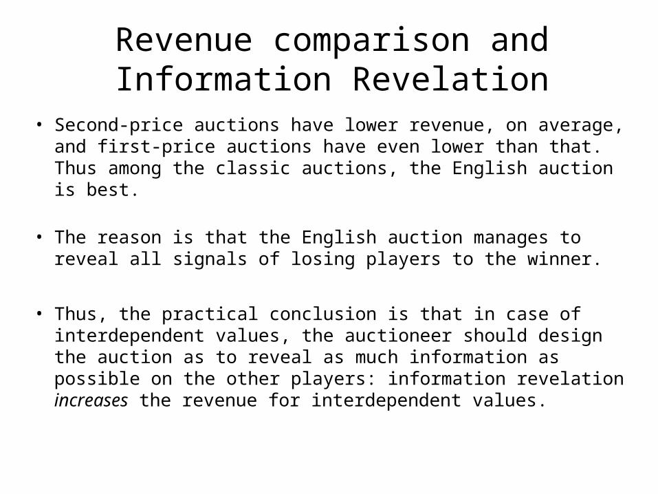
• Second-price auctions have lower revenue, on average, and first-price auctions have even lower than that. Thus among the classic auctions, the English auction is best.
• The reason is that the English auction manages to reveal all signals of losing players to the winner.
• Thus, the practical conclusion is that in case of interdependent values, the auctioneer should design the auction as to reveal as much information as possible on the other players: information revelation increases the revenue for interdependent values.

Social Efficiency• Efficiency: the item goes to the player with highest value.
Measures the society’s welfare, not for the auctioneer’s own utility.
• Why is this good? For example,
– In the FCC auction, the US law requires the government to maximize the efficiency, and not the revenue.
– Super-huge firms sometime have “dummy money” to make inside decisions more efficient (e.g. IBM has “blue-money”).
– Ideological reasons: economists should know how to improve global social welfare.
• With private values, we know that first-price, second-price, and English auction are all efficient. This is true with symmetric interdependent values as well.
• With general interdependent values, this is not the case.

Part 4
• Mechanism design and VCG -- how to “implement” a social choice function.
• Truthful cost-sharing and auctions for unlimited number of identical items.

Two Examples
• “Public Project”: The government considers building a bridge. Each citizen, i, will increase his productivity by some value vi if the bridge will be built. The cost of building the bridge is C. The government wants to build the bridge iff i vi > C, but does not know the values. What to do?
• “Efficient allocation of a resource”: A manager has a unique machine it can give only one of his workers. Each worker, i, will increase his productivity by some value vi. The manager wants to give the machine to the worker with the highest productivity increase. What to do?

The setting
• A social designer has a set of alternatives.
• Each player has a value for every alternative.
• The social planner wants to choose the alternative that maximizes the sum of values.
• Example:
a b c
I 1 5 10
II 7 6 4
III 9 8 7
sum 17 19 21

The setting
• A social designer has a set of alternatives.
• Each player has a value for every alternative.
• The social planner wants to choose the alternative that maximizes the sum of values.
• Example:
a b c
I 1 5 10
II 7 6 4
III 9 8 7
sum 17 19 21 The planner wants to choose alternative c.

Vickrey-Clarke-Groves (VCG)• Problem: the designer does not know the values of the players.
• A solution (VCG mechanism):
– Request players to reveal values.
– Choose the alternative according to players' declarations.
– Charge a payment from player i that is equal to the “damage” she causes the other players: the aggregate value of the best alternative, if player i was absent, minus the sum of values of all players besides i to the chosen alternative.
THM: 1) The VCG mechanism is truthful.
2) Payments are always non-negative (players always pay).
3) A player’s utility is non-negative.4) If the same outcome will be chosen whether the player
participates or not, then his price is zero.

Example
a b c price utility
I 1 5 10 5 10-5=5
II 7 6 4 0 4
III 9 8 7 0 7
sum 17 19 21
If player I is absent, alternative a is chosen, with value 16. The chosen alternative when player I is present is c, and its value to the other players is 11. Thus the price of player I is 16 – 11 = 5.

Example
a b c price utility
I 1 5 10 5 10-5=5
II 7 6 4 0 4
III 9 8 7 0 7
sum 17 19 21
What if player I lies and says that her value for c is 7?
a b c price utility
I 1 5 10 7 2 5-2=3
II 7 6 4
III 9 8 7
sum 17 19 18

Example
a b c price utility
I 1 5 10 5 10-5=5
II 7 6 4 0 4
III 9 8 7 0 7
sum 17 19 21
What if player I lies and says that her value for c is 7?
a b c price utility
I 1 5 10 7 2 5-2=3
II 7 6 4
III 9 8 7
sum 17 19 18
smaller than her utility when telling the truth!

Intuition to proof: Redoing the case of the 2nd price auction
• Another mechanism:
– Each bidder reports his type.
– The winner is the player with the highest value.
– The mechanism pays all other players the winners’ value.
• In other words, we equate the utility of all players to be the highest value.
• Example: three players with true values 10, 8, 7.
10 gets the item, pays nothing; 8, 7 (each) get a payment 10.
• Is this truthful?
• Problem: But we pay the players, instead of getting paid??

Solution
• Solution: subtract a “constant” hi(v-i) from the prices, so that the total will be negative.
• For example: hi(v-i) = max j ≠ i vj . Therefore the payments in the example will be:
– The 10 player will additionally pay max(8,7)=8.
– The 8 player will get 10 and will pay max(10,7)=10, so his total payment will be zero.
– The 7 player will get 10 and will pay max(10,8)=10, so his total payment will also be zero.
– Conclusion: this is exactly the second price auction.

Two main disadvantages of VCG
• Suitable only when our goal is welfare maximization. Other goals, like revenue maximization, are not answered.
• If some values are negative, the mechanism may end up paying the players more than the payments it collects.

Solution to the public project
• Reminder: The government considers building a bridge. Each citizen, i, will increase his productivity by some value vi if the bridge will be built. The cost of building the bridge is C. The government wants to build the bridge iff i vi > C, but does not know the values. What to do?
• We can use VCG. We have two alternatives (YES/NO), and each player, including the government, has a value for each alternative (zero for NO, vi or -C for YES). VCG will choose YES iff i vi - C > 0, which is what the government wants.

Properties of the payments
• A player will pay nothing if j ≠ i vj > C, otherwise (in a YES case) he will pay C - j ≠ i vj.
• These payments may not cover the entire cost C.
• The main problem: suppose C=100, we have 102 players, and each player has value=1. Then the price that each player will pay is zero!
• If we can exclude some players from using the bridge, we can use the CostShare method that we will next see.

Truthful cost sharing
• What happens if we must cover the cost?
• The mechanism CostShare(R): collect bids b1,…,bn, and repeat:
– Suppose we have k bids left (initially we have k=n).
– If there exists a bid lower than R/k, delete it, and repeat.
– Otherwise all remaining bidders win, and each one pays R/k.
• Example: bids (5,4,3,2,1), R=9
– In the 1st round the tentative price is 9/5. Bid 5 is deleted.
– In the 2nd round the tentative price is 9/4. Bid 4 is deleted.
– In the 2nd round the tentative price is 9/3. All three remaining bids win, each one pays 9/3=3. Total revenue is 9.

Properties
• Upon success, we get a revenue R, so for example we will manage to cover the cost of the bridge, if we decide to build it.
• Sometimes we will fail, although the sum of values is larger than the cost.
– Example: two bidders with values 9,2. The cost is 10.
– In other words, this method is not efficient. There is a theorem that if we want efficiency we have to use VCG.
• Another difference from VCG: here we assume we can exclude losers from using the bridge.
• Most importantly, is this truthful??

Truthfulness of CostShare
• Answer: YES!
• Explanation:
– An auction is “value-monotone” if a winner that increases his bid (while the rest stays the same) still wins.
– The “threshold-bid” of a player: the smallest bid for which he still wins (while the rest stays the same).
– Any value-monotone auction, in which every winner pays his threshold-bid, and every loser pays 0, is truthful.
– Example: 2nd price. (What about 1st price)?
– Check at home that CostShare is value-monotone, and every winner indeed pays his threshold bid.

An application: Unlimited Supply
• Infinitely many identical items. Each bidder wants one item.
– Corresponds to a situation were we have no marginal production cost.
– Very common in “digital goods” – songs sold over the Internet, software, etc.
• Bidder i has private value vi for the item.
– We assume throughout that bidders are ordered so thatv1>v2>…>vn

Known probability distribution
• If the values of the players are i.i.d from a probability distribution F, the we can use the optimal auction we already know:
– Since we have unlimited supply, we need to determine, for every bidder separately, if she wins or loses.
– So we need an optimal auction for one bidder.
– We already know that this is a take-it-or-leave-it auction, with a reservation price p such that p=(1-F(p))/f(p)

Worst-case analysis
• What if we do not know, and cannot estimate, the underlying probability distribution?
• We will design an auction with revenue close to the following benchmark auction:
• Suppose we know the values of the players, but must sell all items in the same price. The price will then be:
F(v) = maxi i·vi
• Remark: a non-discriminatory monopoly chooses this price.
• A slightly weaker benchmark: F(2)(v) = maxi>2 i·vi
– For “most” cases F(v)= F(2)(v), and we want to avoid the extreme situations for which this is not true.
• We want to find a small constant c and a truthful auction with revenue R(v) > F(2)(v)/c for any input v.

The auction
1. Randomly partition the bids to two sets (A, B) by tossing a fair coin for each player and associating her to A if the coin came out “head”, and otherwise to B.
2. Compute FA=F(A) and FB=F(B).
3. Run CostShare(A, FB) and CostShare(B, FA) to determine winners and prices.
Theorem: This auction is truthful, no matter what the coin tosses are, and its expected revenue, for any v, is at least F(2)(v)/4.

Part 5
• Multi-item auctions with identical items.
• Multi-item auctions with different items.

Identical items
• Three possible bidder types:
– Unit-demand bidders
– Decreasing marginal values
– General valuations

Unit demand bidders• Each bidder desires one item.
• Two popular “sealed-bid” auction formats:
– Uniform-price auctions: The M highest bidders win, each pays the M+1 highest bid.
– Discriminatory auctions: The M highest bidders win, each pays her bid.
• Two equivalent “open-cry” auctions:
– Ascending price (English): The price ascends until M bidders remain.
– Descending price (Dutch): The price descends until M bidders accept.
• Similarly to the single-item case, uniform-price is equivalent to English, and Discriminatory price is equivalent to Dutch.

Example
• Two items, three bidders, with values 4,7,10:
– The players with values 7,10 win, and each one pays 4.

Example “Real” Applications
• Government securities were sold by the US government using discriminatory auctions, until 1992.
• From 1992, some securities (e.g. 2-years and 5-years) are being sold using a uniform-price auction.
• In the UK, electricity generators bid to sell their output on a daily basis. Until 2000 the auctions were uniform-price, and after that they switched to discriminatory price

Efficiency and Revenue in Unit-Demand
• In uniform-price: is in fact a VCG mechanism (check at home). Therefore:
– Truth-telling is a dominant strategy
– The resulting allocation is efficient
• The revenue equivalence theorem and the optimal auction analysis can be extended to unit-demand bidders:
– Any two auctions with the same outcome in equilibrium raise the same revenue (e.g. unifrom-price and discriminatory-price).
– The optimal auction is to sell the M items to the M bidders with the highest virtual valuations.

Decreasing Marginal Valuations• Each player has a marginal valuation function vi: {1,…,M}-> R
– The value of receiving q items is vi(1)+…+vi(q)
• Marginal decreasing means: vi(q+1) < vi(q) for any 1<q<M
• Implication: Every bidder submits many bids
• Example for the uniform-price auction with two items:
Red is player 1 17
Black is player 2 15
Blue is player 3. 14
Result: the red player wins two items 7
and pays 2·14=28 => utility=4 6
Can one of the players improve his utility??
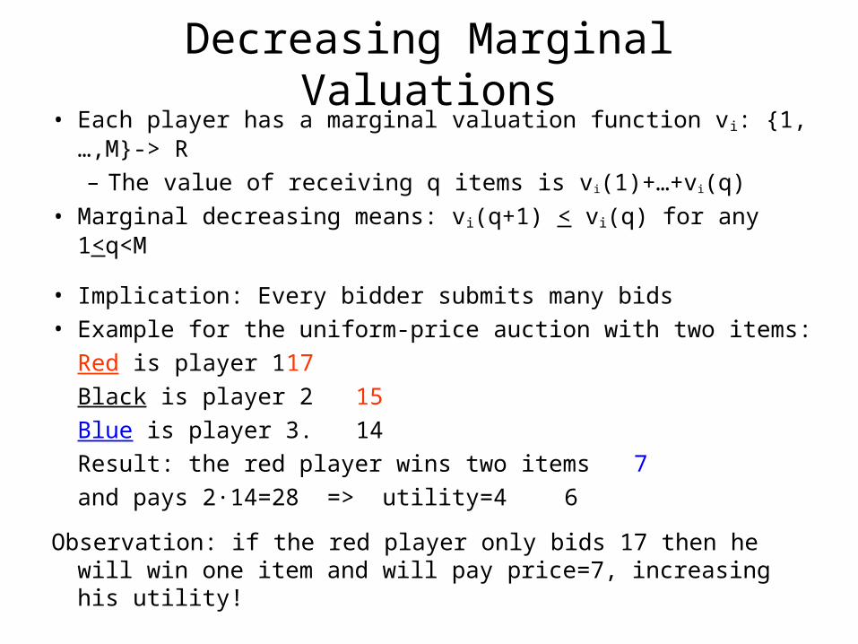
Decreasing Marginal Valuations• Each player has a marginal valuation function vi: {1,…,M}-> R
– The value of receiving q items is vi(1)+…+vi(q)
• Marginal decreasing means: vi(q+1) < vi(q) for any 1<q<M
• Implication: Every bidder submits many bids
• Example for the uniform-price auction with two items:
Red is player 1 17
Black is player 2 15
Blue is player 3. 14
Result: the red player wins two items 7
and pays 2·14=28 => utility=4 6
Observation: if the red player only bids 17 then he will win one item and will pay price=7, increasing his utility!
Conclusions and remarks• It is no longer true that the dominant strategy of a player in the
uniform-price auction is to bid truthfully.
• As we saw, it is beneficial for the players to decrease their stated values for the items. This phenomena is termed “demand reduction”.
• There are no dominant strategies. However, the uniform-price auction is known to have a pure strategy equilibrium, in which:
– “demand reduction” occurs.
– the result is inefficient.
• It is also possible to show that every equilibrium of the discriminatory auction is inefficient.

VCG• VCG continues to have dominant strategies and an efficient
outcome.
• The VCG price for this case: suppose player i won q items, and let x1,…,xq be the q highest non-winning bids of the other players. Then player i pays x1+…+xq.
• In the previous example (2-item auction), 17
15
Result: the red player wins two items 14
and pays 14+7=21 => utility=11 7
6

The residual supply, and the Ausubel auction
• di(p) = max {q | vi(q) > p }
• s-i(p) = M - Σj≠i dj(p)
• 1 bids: 17, 15. 2 bids: 14, 6. 3 bids: 7.
• While price < 6, the demand of player 1 is 2, the demand of player 2 is 2, and the demand of player 3 is 1. Therefore the residual supply of each player < 0.
• At a price=6, 2’s demand decreases to 1. Therefore 1’s residual supply is 0.
• At a price=7, 3’s demand decreases to 0. Therefore 1’s residual supply is 1. Therefore he gets one item at price 7.
• At price=14, 2’s demand decreases to 0. Therefore 1’s residual supply is 1. Therefore he gets a second item for a price 14.

This is equivalent to the VCG prices. As a result, truthfulness is an ex-post equilibrium in this auction.
bidss-i(p)di(p)
VCG price
bids
quantity
s-i(p)di(p)
uniform price
quantity

General valuations (with complementarities)
• In general, marginal valuations may increase. For example v(1)=0, v(2)=100 represents a situation where the player must get two units in order to obtain any value from the items.
• In this case, the discriminatory-price and the uniform-price have no real meaning.
• VCG, again, has dominant strategies, and reaches the efficient outcome. However, no “natural” way of representing VCG or its price is known. We simply use the general mechanism.

Multi-item (“combinatorial”) auctions
• We have M different items.
• Players value subsets of items: vi (S) is the value for subset S. It is usually assumed that:
– Normalization: vi() = 0
– Free disposal: S T => vi(S) < vi(T)
• This represents different types of interactions among the items:
– Substitutability: item “a” can substitute item “b”. For example, an e-store on eBay sells different types of cell phones. In this case we would expect v({a,b}) < v(a) + v(b).
– Complementarities: item “a” helps to extract more value from item “b”. For example, different computer parts. In this case we would expect v({a,b}) > v(a) + v(b).

Real world applications• An early documentation in the beginning of the 20th century: a
company went bankrupt, had to sell two plants (say A and B), and requested price offers. One offer stated a price x for A, a price y for B, and: “if we were to receive A and B, then our price is z” where z > x+y.
• The London bus routes market: 800 routes are auctioned to bus companies, by the 1984 “Transport Act”.
– First auction in 1985, until 1995 half of the network was auctioned at least once. Today 15%-20% of the network is auctioned each year.
• Spectrum rights: hundreds of spectrum intervals, combinations of wave lengths are needed for technical reasons.
– Spectrum auctions are conducted in the US, UK, Europe.

The representation issue
• There are 2M subsets (“bundles”), so each player “holds” many numbers. How should she communicate with the auctioneer?
– With 100 items the total size of the valuation is enormous.
• Two approaches:
– “Bidding languages”: the player writes down her values in a “sophisticated” language that may reduce the total size
– “Iterative queries”: the auctioneer repeatedly asks questions, the answers keep the process going until we reach a result.
• In single-item auctions we also saw these two approaches but here things get complicated.

The strategic issue by an example
a bItem
Temp. winner
Temp. price
-- --
0 0
Player I: v(a)=v(b)=3, v(a,b)=3
Player II: v(a)=v(b)=5, v(a,b)=5
Player III: v(a)=2, v(b)=0, v(a,b)=2
=1

Example
a bItem
Temp. winner
Temp. price
I --
1 0
(phase 1)
=1
Player I: v(a)=v(b)=3, v(a,b)=3
Player II: v(a)=v(b)=5, v(a,b)=5
Player III: v(a)=2, v(b)=0, v(a,b)=2

Example
a bItem
Temp. winner
Temp. price
I II
1 1
(phase 2)
=1
Player I: v(a)=v(b)=3, v(a,b)=3
Player II: v(a)=v(b)=5, v(a,b)=5
Player III: v(a)=2, v(b)=0, v(a,b)=2

Example
a bItem
Temp. winner
Temp. price
III II
2 1
(phase 3)
=1
Player I: v(a)=v(b)=3, v(a,b)=3
Player II: v(a)=v(b)=5, v(a,b)=5
Player III: v(a)=2, v(b)=0, v(a,b)=2

Example
a bItem
Temp. winner
Temp. price
I II
3 1
(phase 4)
=1
Player I: v(a)=v(b)=3, v(a,b)=3
Player II: v(a)=v(b)=5, v(a,b)=5
Player III: v(a)=2, v(b)=0, v(a,b)=2

Example
a bItem
Temp. winner
Temp. price
I II
3 1
(phase 4)
Player I did not bid for the item with lowest price.
=1
Player I: v(a)=v(b)=3, v(a,b)=3
Player II: v(a)=v(b)=5, v(a,b)=5
Player III: v(a)=2, v(b)=0, v(a,b)=2

Example
a bItem
Temp. winner
Temp. price
I II
3 1
Result:
Player I wins item 1 and pays 3.
Player II wins item 2 and pays 1.
=1
Player I: v(a)=v(b)=3, v(a,b)=3
Player II: v(a)=v(b)=5, v(a,b)=5
Player III: v(a)=2, v(b)=0, v(a,b)=2

Properties of the auction
DFN: A player is myopic if he always bids on the item x in argmaxxS [ v(x) - p(x) ]
THM: Assume all players are unit demand. Then:
• When all players are myopic then the ascending auction terminates in an allocation with maximal welfare*.
• When all other players are myopic, player i will maximize* his utility by behaving myopically.
* up to a difference of about .
• In the previous example, suppose is negligible, then players I and II will win and will both pay price=2, which is exactly the VCG price.

What happens with complementarities?
• Example: Two items a,b are for sale. Bidder 1 needs both, for a value of 140. Bidder 2 needs only one (either a or b), for a value of 75.
– Suppose we change the ascending auction by simply allowing the bidders to place their name on several items together.
– We would like bidder 1 to win. However, bidder 2 raises the prices of both items to 75, so in order to win bidder 2 needs to pay 150, which is too much for him.
– This is called the “exposure” problem.

Package bidding
• We can attempt to solve this by introducing prices for bundles, and not only for items.
– In our example, we will have three prices: for {a}, for {b}, and for {ab}.
– Note that we have exponential number of prices.
• The course of the auction:
– Bidders state all bundles for which price < value.
– The seller composes an allocation with maximal value.
– Prices on all bundles desired by a losing player are increased
• This will solve the exposure problem:
– The prices on all bundles will reach 75, and then stop.

Package bidding (2)• Package bidding creates another problem:
– Suppose a third bidder that wants item {b} for 40. We would then like bidders 2+3 to win.
– Now, the prices for {a} and {b} will advance more slowly, as the winning allocation can contain both {a} and {b}.
– At some point, the prices may be 40 for {a}, 40 for {b}, and {80} for {a,b}. Now, player 2 will not be willing to increase his bid for {a}, as she’s hoping that player 3 will do this first for {b}, and so nobody raises the bid for the singletons, and player 1 wins.
• This is called the “threshold” problem.
• This can be solved by having bundle prices for each bidder separately. This turns out to be equivalent to VCG.

The disadvantages of VCG• Exponential complexity (both communication and computation).
• Low and non-monotonic seller’s revenue :
– Example: Bidder 1 wants {a,b} for 2M. Bidders 2,3 value any singleton {a} or {b} by 2M. In VCG 2 and 3 are the winners.
– The price of bidder 2 is the difference between the value, to the other bidders, of one item or two items. But this is zero!
– So the revenue is zero. If the two items were bundled and sold as a whole, we would get a price of 2M.
– Removing the third bidder will increase the revenue.
• Collusion: If bidders 2,3 were to have values 0.5M, they were losing. But, if together they would have raised their values to 2M, they would win, and would pay zero, i.e. gaining from the lie.
• Shill bidding: If there were no bidder 3, bidder 2 will profit from “inventing” him.

So what happens in practice?
• Ascending auctions are usually the choice, despite their problems.
• The FCC runs a “Simultaneous Ascending Auction” (SAA), where prices are per item.
• A “clock auction” aims to resolve the threshold problem by increasing prices in a constant rate (“clock”).
– Sometimes people add “activity rules”, e.g. the demand of a player must be consistent among different rounds and prices.
• The “clock-proxy” auction format suggests to perform a clock auction, followed by a package bidding concluding phase.
• Those are all heuristics, with incomplete theoretical background, and much more research is still needed.