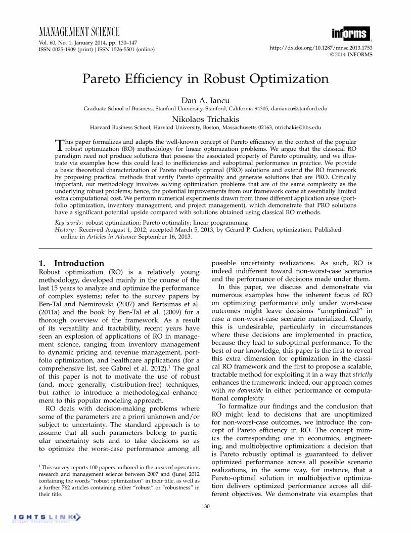
MANAGEMENT SCIENCEVol. 60, No. 1, January 2014, pp. 130–147ISSN 0025-1909 (print) ó ISSN 1526-5501 (online) http://dx.doi.org/10.1287/mnsc.2013.1753

©2014 INFORMS

Pareto Efficiency in Robust OptimizationDan A. Iancu

Graduate School of Business, Stanford University, Stanford, California 94305, daniancu@stanford.edu

Nikolaos TrichakisHarvard Business School, Harvard University, Boston, Massachusetts 02163, ntrichakis@hbs.edu

This paper formalizes and adapts the well-known concept of Pareto efficiency in the context of the popularrobust optimization (RO) methodology for linear optimization problems. We argue that the classical RO

paradigm need not produce solutions that possess the associated property of Pareto optimality, and we illus-trate via examples how this could lead to inefficiencies and suboptimal performance in practice. We providea basic theoretical characterization of Pareto robustly optimal (PRO) solutions and extend the RO frameworkby proposing practical methods that verify Pareto optimality and generate solutions that are PRO. Criticallyimportant, our methodology involves solving optimization problems that are of the same complexity as theunderlying robust problems; hence, the potential improvements from our framework come at essentially limitedextra computational cost. We perform numerical experiments drawn from three different application areas (port-folio optimization, inventory management, and project management), which demonstrate that PRO solutionshave a significant potential upside compared with solutions obtained using classical RO methods.

Key words : robust optimization; Pareto optimality; linear programmingHistory : Received August 1, 2012; accepted March 5, 2013, by Gérard P. Cachon, optimization. Published

online in Articles in Advance September 16, 2013.

1. IntroductionRobust optimization (RO) is a relatively youngmethodology, developed mainly in the course of thelast 15 years to analyze and optimize the performanceof complex systems; refer to the survey papers byBen-Tal and Nemirovski (2007) and Bertsimas et al.(2011a) and the book by Ben-Tal et al. (2009) for athorough overview of the framework. As a resultof its versatility and tractability, recent years haveseen an explosion of applications of RO in manage-ment science, ranging from inventory managementto dynamic pricing and revenue management, port-folio optimization, and healthcare applications (for acomprehensive list, see Gabrel et al. 2012).1 The goalof this paper is not to motivate the use of robust(and, more generally, distribution-free) techniques,but rather to introduce a methodological enhance-ment to this popular modeling approach.RO deals with decision-making problems where

some of the parameters are a priori unknown and/orsubject to uncertainty. The standard approach is toassume that all such parameters belong to partic-ular uncertainty sets and to take decisions so asto optimize the worst-case performance among all

1 This survey reports 100 papers authored in the areas of operationsresearch and management science between 2007 and (June) 2012containing the words “robust optimization” in their title, as well asa further 762 articles containing either “robust” or “robustness” intheir title.

possible uncertainty realizations. As such, RO isindeed indifferent toward non-worst-case scenariosand the performance of decisions made under them.In this paper, we discuss and demonstrate via

numerous examples how the inherent focus of ROon optimizing performance only under worst-caseoutcomes might leave decisions “unoptimized” incase a non-worst-case scenario materialized. Clearly,this is undesirable, particularly in circumstanceswhere these decisions are implemented in practice,because they lead to suboptimal performance. To thebest of our knowledge, this paper is the first to revealthis extra dimension for optimization in the classi-cal RO framework and the first to propose a scalable,tractable method for exploiting it in a way that strictlyenhances the framework: indeed, our approach comeswith no downside in either performance or computa-tional complexity.To formalize our findings and the conclusion that

RO might lead to decisions that are unoptimizedfor non-worst-case outcomes, we introduce the con-cept of Pareto efficiency in RO. The concept mim-ics the corresponding one in economics, engineer-ing, and multiobjective optimization: a decision thatis Pareto robustly optimal is guaranteed to deliveroptimized performance across all possible scenariorealizations, in the same way, for instance, that aPareto-optimal solution in multiobjective optimiza-tion delivers optimized performance across all dif-ferent objectives. We demonstrate via examples that

130

Dow

nloa

ded

from

info

rms.o

rg b

y [1

71.6

6.19

.162

] on

12 N

ovem

ber 2

014,

at 1

0:19

. Fo

r per

sona

l use

onl

y, a

ll rig

hts r

eser

ved.

Iancu and Trichakis: Pareto Efficiency in Robust OptimizationManagement Science 60(1), pp. 130–147, © 2014 INFORMS 131

decisions made using RO need not have this property.To alleviate this, we propose methods for verifyingwhether a decision is Pareto optimal or not and meth-ods for obtaining robustly optimal decisions that areprovably Pareto optimal as well. Put differently, inthis paper, we introduce an essential property that ROdecisions that are to be implemented in practice needto possess (in a way that parallels the importance ofPareto efficiency in economics) and develop theoryand computational tools pertaining to it. Our method-ology enables a decision maker to compute robustlyoptimal solutions that are compatible with the classi-cal RO framework, incur no extra computational cost,and can perform strictly better in practice.Specifically, we make the following contribu-

tions:a. We formalize and adapt the well-accepted con-

cept of Pareto efficiency to the classical RO frame-work. We demonstrate that the framework neednot produce solutions that possess the associatedproperty of Pareto optimality, and we illustrate viaexamples how this could lead to inefficiencies andsuboptimal performance in practice.b. We provide a basic theoretical characterization

of Pareto robustly optimal solutions.c. We extend the RO framework by proposing prac-

tical methods that verify Pareto optimality and gen-erate solutions that are also (provably) Pareto. Crit-ically important, all of our proposed methodologyinvolves optimization problems that are of the samecomputational complexity as the underlying robust prob-lems; hence, the potential improvements from ourframework come at essentially limited extra computa-tional cost.d. We perform numerical experiments drawn from

three different application areas studied in the man-agement science literature: portfolio optimization,inventory management, and project management. Thestudies demonstrate that Pareto robustly optimalsolutions obtained using our methodology have a sig-nificant upside compared with solutions obtained viaclassical methods.We conclude by noting that our treatment in this

paper is restricted to the case of uncertain linear opti-mization problems. We make this choice primarilybecause of the overwhelming preponderance of lin-ear models in practice, as well as for reasons of sim-plicity and ease of exposition. However, we see thisas a first step in treating more general optimizationproblems appearing in the classical RO framework(Ben-Tal et al. 2009).

1.1. Literature ReviewOriginally introduced in operations research and man-agement science by Soyster (1973), the RO method-ology has been revitalized in the late 1990s and

early 2000s through the seminal work of Ben-Tal andNemirovski (2002), Bertsimas and Sim (2003), andEl-Ghaoui et al. (1998) (see the review papers byBen-Tal andNemirovski 2007 andBertsimas et al. 2011aand the book by Ben-Tal et al. 2009 for a thoroughoverview of the methodology and contributions).With a strong emphasis on computational tractabil-

ity and the ability to accommodate a diverse rangeof relevant optimization models, the RO methodologyhas been adopted in many applications of interest inmanagement science. Such examples include inven-tory management (Ben-Tal et al. 2005, Bertsimas andThiele 2006, Bienstock and Özbay 2008, See and Sim2010, Bertsimas et al. 2011b), dynamic pricing and rev-enue management (Adida and Perakis 2006, Lim andShanthikumar 2007, Perakis and Roels 2010), assort-ment planning (Rusmevichientong and Topaloglu2012), portfolio optimization (Goldfarb and Iyengar2003, Fabozzi et al. 2007, Bertsimas and Pachamanova2008), project management (Cohen et al. 2007, Adidaand Joshi 2009, Goh et al. 2010, Wiesemann et al.2012), healthcare (Chan et al. 2006), and auctiondesign (Bandi and Bertsimas 2012). The list is by nomeans exhaustive; the interested reader can refer tothe recent review papers by Bertsimas et al. (2011a)and Gabrel et al. (2012) and the book by Ben-Tal et al.(2009) for comprehensive references.Despite its empirical success, however, the robust

framework has been known to suffer from severalpotential shortcomings. One criticism is that by focus-ing exclusively on the worst-case outcomes, it mayresult in conservative decisions, with limited poten-tial upside. This has led to several alternative pro-posals of robustness measures, such as absoluteor relative regret (Savage 1972), “soft-robustness”(Ben-Tal et al. 2010), “light-robustness” (Fischetti andMonaci 2009), bw-robustness (Roy 2010, Gabrel et al.2013), Å-robustness (Kalai et al. 2012), among oth-ers. Depending on the exact assumptions and setup,such approaches typically result in the same (orslightly decreased) modeling flexibility and the same(or slightly increased) computational complexity asthe standard RO framework. Critically, however, allsuch approaches trade off some of the robustness (i.e.,performance in the worst case) in exchange for poten-tial upside. By contrast, our approach, which parallelsthe notion of Pareto efficiency, guarantees the sameworst-case outcome while at the same time allowingpotentially improved upside, with no increase in com-putational complexity.A second and more subtle criticism is that by solely

focusing on worst-case outcomes, the minimax/maximin criterion may result in multiple optimalsolutions, and hence it may generate Pareto inefficien-cies in the decision process. This idea has emergedin several research streams, from fairness in resourceallocation (Young 1995, Bertsimas et al. 2012) to

Dow

nloa

ded

from

info

rms.o

rg b

y [1

71.6

6.19

.162

] on

12 N

ovem

ber 2

014,

at 1

0:19

. Fo

r per

sona

l use

onl

y, a

ll rig

hts r

eser

ved.

Iancu and Trichakis: Pareto Efficiency in Robust Optimization132 Management Science 60(1), pp. 130–147, © 2014 INFORMS

multiobjective optimization (Ogryczak 1997, Suh andLee 2001), but it has been, to the best of our knowl-edge, absent from the mainstream RO literature.2 Theunifying characteristic in the above settings is thatthey are concerned with a finite set of alternativerealizations/scenarios (e.g., the multiple parties in aproblem of equitable resource allocation or the objec-tives in a multiobjective problem). This case, how-ever, is typically of limited interest in RO, where thestandard setup involves a continuous uncertainty set,i.e., an infinite number of realizations (Ben-Tal et al.2009). In this sense, the proposals for correcting Paretoinefficiencies of the maximin rule in resource alloca-tion and multiobjective optimization (e.g., the lexico-graphic max–min fairness scheme; see Young 1995,Ogryczak 1997) cannot be readily extended to theclassical RO framework. By contrast, our definitionof Pareto robustly optimal solutions is applicable tocases with both finite and infinite uncertainty sets,and hence fully compatible with the RO methodol-ogy. Furthermore, our approach still allows potentialmultiplicity in the Pareto robustly optimal solutions,hence not eliminating the benefits of multiplicity inRO (Bertsimas et al. 2013, Iancu et al. 2013).Finally, we note that the concepts of “Pareto opti-

mality/efficiency” and “robust optimization” haveappeared together before, typically in the area ofmultiobjective optimization, but in a very differ-ent spirit than that addressed in the present paper.In particular, Gorissen and den Hertog (2011) discussthe use of RO and, more broadly, convex optimiza-tion to approximate the Pareto frontier in multiob-jective optimization problems. Several papers havealso attempted introducing robust formulations ofmultiobjective problems (e.g., Suh and Lee 2001, Deband Gupta 2005, Cristobal et al. 2006, Luo and Zheng2008, Ono and Nakayama 2009, Chen et al. 2012).The notions of robustness used are typically differentthan those in the classical RO framework, resultingin models that require solving very difficult optimiza-tion problems; this usually leads to the use of variousheuristics, such as evolutionary algorithms, polyno-mial chaos, or particle swarm optimization.

1.2. NotationWe use 1 to denote the vector with all componentsequal to 1. We use e

i

to denote the unit vector with 1in the ith component. The inequality sign for vectorsis used for component-wise inequality.We use several basic notions of convex analysis

(Rockafellar 1970) that we denote as follows. For a setS ⇢✓n, we use ext4S5 to denote the set of its extreme

2 The multiplicity of optimal solutions has been typically seen as apositive feature in RO, because it allowed deriving simple dynamicpolicies in multiperiod problems (Bertsimas et al. 2010, Iancu et al.2013) or optimizing secondary objectives (Bertsimas et al. 2013).

points, we use conv4S5 to denote its convex hull, weuse ri4S5 to denote its relative interior, and we use S

⇤

to denote its dual cone.

2. Pareto Robustly Optimal SolutionsIn this section, we introduce and formally define thenotion of Pareto efficiency in RO. For illustration pur-poses and to ease exposition, we consider a specificform of RO problems, for which we present our def-initions and the results in §3. In §4, we discuss howour findings extend to more general forms of ROproblems.The type of RO problem we consider is a linear

optimization problem where only the objective is sub-ject to uncertainty. Specifically, we consider the prob-lem of selecting x from a polyhedral feasible set X ⇢✓n so as to maximize p

T

x. The objective vector p is apriori unknown and belongs to a polyhedral uncer-tainty set U ⇢✓n. We assume that both sets X and U

are nonempty and bounded and that their inequalityrepresentations are

X = 8x 2✓n

2 Ax b9 and (1a)

U = 8p 2✓n

2 Dp� d91 (1b)

where A 2✓m

X

⇥n, b 2✓m

X , D 2✓m

U

⇥n, and d 2✓m

U aregiven. We note that our findings readily extend to thecase where we only have access to a representation ofU through its extreme points.Although linear models with polyhedral uncer-

tainty sets are a strict subset of the RO methodology,we choose them as the focus of our treatment dueto their widespread use in practice, and because theyare a natural first step before examining more generalconvex optimization models.According to the classical RO paradigm (Ben-Tal

et al. 2009), one selects x in the above setting by solv-ing the following optimization problem:3

maximizex2X

minp2U

p

T

x0 (2)

To solve this problem, note that min8pT x2 p 2 U 9 =max8yT

d2 D

T

y = x1y � 09, by strong linear pro-gramming duality. Therefore, letting z

RO denote theoptimal value and letting X

RO denote the set of opti-mal solutions of problem (2), it is easy to check that

X

RO = �x 2X2 9y 2✓m

U+ such that

D

T

y = x1 y

T

d � z

RO 0 (3)

3 Note that this model can also correspond to a distributionallyrobust setting, where U is a subset of the probability simplex,denoting ambiguity about the true probability measure, and thegoal is to maximize the worst-case expected outcome (where natureis choosing the distribution adversarially). In this sense, our modelcan speak to the vast literature on risk measures and choice underambiguity (see, e.g., Ben-Tal et al. 2010 or Bertsimas et al. 2011a formore references).

Dow

nloa

ded

from

info

rms.o

rg b

y [1

71.6

6.19

.162

] on

12 N

ovem

ber 2

014,

at 1

0:19

. Fo

r per

sona

l use

onl

y, a

ll rig

hts r

eser

ved.

Iancu and Trichakis: Pareto Efficiency in Robust OptimizationManagement Science 60(1), pp. 130–147, © 2014 INFORMS 133

An optimal solution x 2 X

RO of problem (2) is typi-cally referred to as a robustly optimal solution in thissetting. It corresponds to a solution that maximizesthe worst-case objective value p

T

x under all possiblerealizations of the uncertainty p 2 U . In other words,a robustly optimal solution is selected under the solerequirement of protecting us against worst-case sce-narios. We are guaranteed that no other solution doesbetter along that requirement. If such a solution is tobe used in practice, however, this raises the followingquestions.• How would x perform (in terms of the objective

value) in case the uncertainty scenario that actuallymaterialized did not correspond to a worst-case one?• Are there any guarantees that no other solution

exists that, apart from protecting us from worst-casescenarios, also performs better overall, under all pos-sible uncertainty realizations?To better understand the meaning of these ques-

tions, we consider a stylized network flow examplearising in a communication network. The exampleillustrates that, in general, a robustly optimal solutionx 2 X

RO might perform poorly in case a worst-casescenario was not realized: in fact, we show that it issometimes possible to find another robustly optimalsolution that outperforms x under all possible uncer-tainty realizations.

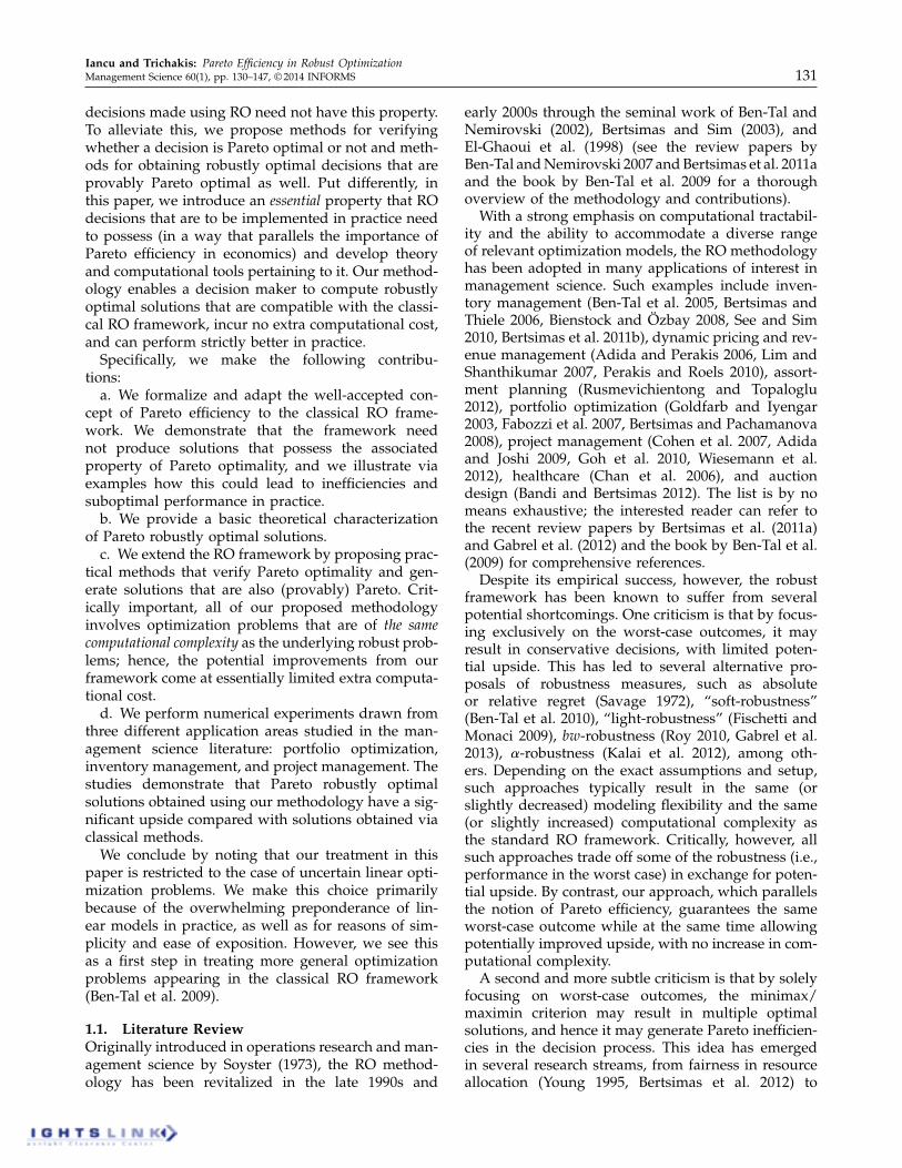
Example 1. Consider a communication networkthat consists of multiple links. Any given link is usedto transmit information between two points in thenetwork at a rate that is determined by the network

Figure 1 An Illustration of the Network Structure in Example 1

Channel ALink l1

Link l0

Link l2

x1 = a1

x2 = a2 + b2

a0

a1

a2

Channel BLink l3

Link lN + 2

x3 = b3

xN + 2 = bN + 2

b2

bN + 2

b3

......

... ...

manager. The links share different capacitated com-munication channels for transmission; capacity limi-tations then affect the information transmission ratesof the individual links.Specifically, consider the following network struc-

ture: there are two channels, denoted by A and B.The channels are of unit capacity and are utilized byN + 3 links, denoted by l01 l11 0 0 0 1 lN+2, with N � 3.Links l0 and l1 utilize only channel A. Link l2 uti-lizes both channels A and B. Links l31 0 0 0 1 lN+2 utilizeonly channel B. Let a

i

denote the transmission rateof link l

i

over channel A, i = 01112. Accordingly, bi

denotes the transmission rate of link l

i

over channel B,i = 21 31 0 0 0 1N + 20 Vectors a 2 ✓3 and b 2 ✓N+1 con-tain the associated values. The structure is depicted inFigure 1.Links l11 0 0 0 1 lN+2 are dedicated for emergency pur-

poses, whereas link l0 is used for general purposes.Let x

i

be the transmission rate of the emergencylink l

i

, i= 1121 0 0 0 1N + 2. We have

x1 = a11 x2 = a2 + b21 and

x

i

= b

i

1 i= 3141 0 0 0 1N + 20

In case an emergency transmission needs to be esta-blished, this is achieved by utilizing one of the dedi-cated links or a combination thereof. More specifically,let f

i

be the fraction of the emergency transmissionrouted via link l

i

, i = 1121 0 0 0 1N + 2. The net emer-gency transmission rate is then

f

T

x=N+2X

i=1

f

i

x

i

0

Dow

nloa

ded

from

info

rms.o

rg b

y [1

71.6

6.19

.162

] on

12 N

ovem

ber 2

014,

at 1

0:19

. Fo

r per

sona

l use

onl

y, a

ll rig

hts r

eser

ved.

Iancu and Trichakis: Pareto Efficiency in Robust Optimization134 Management Science 60(1), pp. 130–147, © 2014 INFORMS

Fractions f depend on the emergency situation andare uncertain. In particular, f is assumed to belong toa probability simplex uncertainty set U ; i.e.,

U = �f 2✓N+2

+ 2 1T f = 1 0

The problem for the network manager is then to selectrates x, a, and b (in case of an emergency) so asto maximize the net emergency transmission rate. Ifthe manager uses robust optimization, the rates areselected by solving

maximize minf2U

f

T

x

subject to x1 = a11

x2 = a2 + b21

x

i

= b

i

1 i= 31 0 0 0 1N + 21

a0 + a1 + a2 = 11

b2 + b3 + · · ·+ b

N+2 = 11

a1 b � 01

(4)

with variables x, a, and b. Let X be the feasible set.It is easy to check that the optimal value is zRO = 1/N ,and the optimal set is

X

RO =⇢4x1a1 b5 2X2 x� 1

N

1�0

To solve problem (4), we used the standard ROmethodology introduced in §2 and solved the result-ing linear program using interior point methods.4 Fora problem with N = 10, we obtained the followingrobustly optimal solution:

a

IP = ⇥ 13

13

13

⇤T

1 b

IP = ⇥0 1

10 · · · 110

⇤T

1

x

IP = ⇥ 13

13

110 · · · 1

10

⇤T

0

Note that for any realization of f drawn from U , wehave

f

T

x

IP � 1N

= 110

0

An associated worst-case realization of f for whichthe obtained performance is equal to 1/10 is, forinstance, e3. Consider now a non-worst-case scenariofor xIP, e.g., f = e1. Then, the realized objective valueis e

T

1 xIP = 1/3.

We now compare the robustly optimal solution4x

IP1a

IP1 b

IP5 that we obtained with the following

solution:

x

? = ⇥ 12

12

110 · · · 1

10

⇤T

1

a

? = ⇥0 1

212

⇤T

1 b

? = ⇥0 1

10 · · · 110

⇤T

0

It is easy to check that this solution is also robustlyoptimal; i.e., 4x?

1a

?

1 b

?

5 2X

RO. Hence, it has the same

4 More specifically, the SeDuMi software package (Sturm et al. 2006)was used.

qualities as the obtained solution 4x

IP1a

IP1 b

IP5 in pro-

tecting us from worst-case realizations of f . However,if f = e1 is realized, this solution yields strictly betterperformance:

e

T

1 x? = 1

2 > e

T

1 xIP = 1

3 0

In fact, it is easy to see that x? performs strictly betteror at least as well as xIP for any realization of f drawnfrom U . In particular, we have

f

T

x

? � f

T

x

IP1 8 f 2U 1 and (5a)

f

T

x

?

> f

T

x

IP1 8 f 2U \ 8f 2 f1 + f2 > 090 (5b)

The above discussion demonstrates that by focus-ing only on worst-case scenarios, the classical ROparadigm allows solutions that are dominated, i.e., thatcan be improved without affecting worst-case perfor-mance. Clearly, this inefficiency is not important incase RO is used only for purposes of determining theoptimal worst-case costs or profits. However, it mightnegatively affect managers who utilize RO to actuallycompute solutions they implement in practice.To rectify the aforementioned weakness of the clas-

sical RO framework, we need to additionally requirefrom a robustly optimal solution to perform as wellas possible across all uncertainty scenarios that canbe realized. In particular, for any robustly optimalsolution we select, we need to guarantee that theredoes not exist another solution that performs atleast as well across all uncertainty realizations andstrictly better at some realizations. If such a solutionexisted, it would be strictly preferred for all practicalconsiderations.We call solutions with the above property Pareto

robustly optimal (PRO) solutions. Formally, we havethe following definition.

Definition 1. A solution x is a Pareto robustlyoptimal solution for problem (2) if it is robustly opti-mal, i.e., x 2X

RO, and there is no other x 2X such that

p

T

x� p

T

x1 8p 2U 1 and

p

T

x > p

T

x1 for some p 2U 0

In the definition above, we say that x Paretodominates x. As discussed in the introduction, theterminology we use borrows from economics andmultiobjective optimization: RO can be viewed asa multiobjective optimization problem with an infi-nite number of objectives, one for each uncertaintyscenario.Returning to Example 1, by (5), we have that the

solution 4x

?

1a

?

1 b

?

5 Pareto dominates the solution x

IP.Moreover, one can show that the solution 4x

?

1a

?

1 b

?

5 is

Dow

nloa

ded

from

info

rms.o

rg b

y [1

71.6

6.19

.162

] on

12 N

ovem

ber 2

014,

at 1

0:19

. Fo

r per

sona

l use

onl

y, a

ll rig

hts r

eser

ved.

Iancu and Trichakis: Pareto Efficiency in Robust OptimizationManagement Science 60(1), pp. 130–147, © 2014 INFORMS 135

a PRO solution. In fact, if we denote the set of all PROsolutions with X

PRO, then for problem (4) we have

X

PRO = �4x1a1 b5 2X2 x� 1

N

11 x1 + x2 = 1 0

Below is another toy example that illustrates thenotion of PRO solutions.

Example 2. Consider the following problem, whichis of the same form as problem (2):

maximize minp2U

�p1x1 + p2x2 + p3x3

subject to x1 É x2 = 01

x1 + x3 = 01

x1 � 01

x1 11

(6)

where U = 8p 2 ✓32 1 p 29 is a hypercube uncer-

tainty set.For the above problem, it is easy to check that for

any x 2 X, 61 1 27T is a worst-case uncertainty real-ization for which 61 1 27x = 0. Hence, we have thatX =X

RO.To solve problem (6), we used the standard RO

methodology discussed above and solved the result-ing linear program using the simplex method.5

We obtained the robustly optimal solution x

simplex =60 0 07T . Consider the solution x

? = 61 1 É17T . For anyuncertainty realization different from the worst-caserealization we identified above, i.e., p 6= 61 1 27T , wehave that pT x?

> p

T

x

simplex. For the worst-case realiza-tion, both solutions yield an objective value of zero.Hence, solution x

? Pareto dominates solution x

simplex.In fact, x? is the only PRO solution for problem (6), sothat XPRO = 8x

?

9.

There are many interesting questions to be ad-dressed that are theoretically and practically relevantin view of the notion of PRO solutions we have intro-duced. Do PRO solutions always exist, and how canwe find them efficiently? When is every robustly opti-mal solution also a PRO solution? Can we character-ize X

PRO? Is it a convex set?Apart from shedding light on the questions raised

above, the rest of the paper is devoted to answeringthe following two central questions:1. Given a robustly optimal solution x 2 X

RO, howdo we check whether x is also PRO? If it is not, howdo we find a PRO solution x 2X

PRO that Pareto dom-inates x?

5 We used the IBM ILOG CPLEX solver, with the simplex methodselected.

2. How do we optimize over the set of PRO solu-tions X

PRO? From our discussion so far, it should beobvious that for practical decision making, a man-ager should always prefer PRO solutions. In case amanager also has a secondary objective, how can sheselect a PRO solution that is optimal with respect tothis secondary objective?

3. Finding and Optimizing OverPRO Solutions

As suggested at the end of §2, several questions ofinterest can be posed concerning the set of PRO solu-tions. The goal of this section is to provide detailedanswers to these questions. We focus our discussionhere on the class of RO problems described by (2),when the feasible set X and the uncertainty set U

are given by (1a) and (1b), respectively. In §4, werevisit and extend our results to several other modelsof interest.

3.1. Finding PRO SolutionsIn current practice, a decision maker would first for-mulate a RO model for the particular application ofinterest and then seek to solve the resulting prob-lem, hence determining a robustly optimal solutionx 2X

RO. However, as suggested by the simple exam-ples in §2, the solution x does not necessarily have tobe a PRO solution.In this context, the first question of interest is how

to check whether a given x 2X

RO is also PRO and, ifnot, how to find an x that is PRO and Pareto dom-inates x. The following theorem argues that both ofthese questions can be answered in a straightforwardfashion by solving a single linear program (LP) ofcompact size.

Theorem 1. Given a point x 2 X

RO, consider an arbi-trary point p 2 ri4U 5 and the following optimizationproblem:

maximizey

p

T

y

subject to y 2U

⇤1

x+ y 2X0

(7)

Then, either the optimal value in the problem is zero, inwhich case x 2 X

PRO, or the optimal value is strictly pos-itive, in which case x = x + y

? Pareto dominates x andx 2X

PRO for any optimal solution y

?.

Proof of Theorem 1. Note first that y = 0 is alwaysfeasible in problem (7). Hence, the optimal value isnonnegative. The discussion separates into two dis-joint cases.Case 1: The optimal value is zero. Assume that x y

X

PRO; i.e., there exists x 2X that Pareto dominates x.In particular, (i) p

T

x � p

T

x1 8p 2 U , and (ii) 9 p 2 U

such that pT x > p

T

x. Without loss of generality, we can

Dow

nloa

ded

from

info

rms.o

rg b

y [1

71.6

6.19

.162

] on

12 N

ovem

ber 2

014,

at 1

0:19

. Fo

r per

sona

l use

onl

y, a

ll rig

hts r

eser

ved.

Iancu and Trichakis: Pareto Efficiency in Robust Optimization136 Management Science 60(1), pp. 130–147, © 2014 INFORMS

additionally take p 2 ext4U 5, e.g., as a vertex solutionto max

p2U 4xÉ x5

T

p.Note that xÉ x is readily feasible in (7). We claim

that p

T

4x É x5 > 0. To prove this, recall that any p 2ri4U 5 has a representation as a strict convex combi-nation of all extreme points of U (Rockafellar 1970),i.e., 9ã 2 ✓óextU ó such that ã > 01 1Tã = 1, and p =P

i2I ã

i

p

i

, where ext4U 5

def= 8p

i

2 i 2I9. But then,

p

T

4xÉ x5= p

T

4xÉ x5| {z }>0

+ X

i2I 2p

i

6=p

p

T

i

4xÉ x5| {z }�0

> 00

This immediately leads to the desired contradiction.Case 2: The optimal value is positive. The conditions

in Definition 1 can be directly verified for x, show-ing that x Pareto dominates x. To see that x 2 X

PRO,consider testing this by solving problem (7), i.e., withx replaced by x = x + y

?, and the same p. We claimthat the optimal solution to this problem must be zero(which, in turn, implies that x 2 X

PRO). Otherwise,if an optimal solution y existed, with p

T

y > 0, theny

? + y would be feasible and provide a higher objec-tive value than y

? when solving problem (7) to testwhether x was PRO, contradicting the fact that y? wasan optimal solution. ÉLet us comment on the result and its relevance.

We claimed that problem (7) is an LP. This followssince the dual cone U

⇤ of a polyhedral set U alwayshas a polyhedral representation (Rockafellar 1970).For instance, if U is the polytope given by (1b), thenby strong LP duality,

U

⇤ def= 8y 2✓n

2 y

T

p� 01 8p 2U 9

= �y 2✓n

2 9ã 2✓m

U+ such thatD

T

ã= y1 d

T

ã� 0 0 (8)

This implies that problem (7) can be solved effi-ciently using standard software (e.g., CPLEX, Gurobi,SeDuMi) for sizes that are typical in real-worldapplications.Note also that our result is stated for an arbitrary

point p in the relative interior of U , so that prob-lem (7) must only be solved once. Since finding a pointin the relative interior of a polyhedron can be doneefficiently by LP techniques (Schrijver 2000), this read-ily leads to an efficient procedure for testing whetherx 2X

PRO and (if not) for producing points that Paretodominate x.In a different sense, Theorem 1 also confirms that

PRO solutions to any robust LP problem always existand suggests the following procedure for findingthem.

Corollary 1. Consider an arbitrary point p 2 ri4U 5.Then, all the optimal solutions to the problemmaximize

x2XRO pT

x are PRO.

The proof follows analogously to that of Theorem 1and is omitted. It is interesting to note that finding anx 2X

PRO is not substantially more difficult than find-ing an x 2 X

RO—one needs to sample a point p fromri4U 5, which can be done by an LP, and to solve anadditional LP over the set X

RO. That is, although alimited additional overhead is incurred, the computa-tional complexity of the underlying RO framework isfundamentally preserved. Moreover, since the poten-tial gains from working with PRO solutions can besubstantial (as illustrated in our examples in §5), thissuggests that the framework can have considerablepromise in practice.The procedure introduced in Corollary 1 also sug-

gests a simple way to generate (potentially different)solutions in X

PRO, by (i) sampling different valuesp from ri4U 5 and (ii) solving the corresponding LPover X

RO. The following result confirms that all thepoints of X

PRO can, in fact, be generated by such aprocedure.

Proposition 1. For any x2XPRO, there exists p2 ri4U 5

such that x 2 argmaxy2XRO p

T

y.

Proof of Proposition 1. Let P 2 ✓n⇥óext4U 5ó denotethe matrix with columns given by the extreme pointsof U , and without loss of generality, assume that thelast óext4U 5ó É k columns (where k óext4U 5ó) cor-respond to all the points p 2 ext4U 5 such that pT x =z

RO 8x 2X

RO. Also, let P 2✓n⇥k denote the matrixobtained by keeping the first k columns of P .Consider any point x 2 X

PRO. To construct the de-sired p 2 ri4U 5, we note that it is enough to show that9ã 2 ✓k such that ã � 1 and x 2 argmax

y2XRO yT

Pã.The reason is that any such ã can be extended into

ã

def= 11Tã+ óext4U 5ó É k

ã

1

�1

which satisfies the relations ã > 01 1T ã = 1, and x 2argmax

y2XRO yT

P ã if and only if

x 2 argmaxy2XRO

y

T

P

ã

0

�0

To this end, assume (for the purposes of deriv-ing a contradiction) that 8ã � 1, we have x yargmax

y2XRO yT

Pã. This implies that

8ã� 119y4ã5 2X

RO2 4y4ã5É x5

T

Pã> 0 )minã�1

maxy2XRO

4yÉ x5

T

Pã> 04⇤5,

maxy2XRO

minã�1

4yÉ x5

T

Pã> 04⇤⇤5)

9y 2X

RO2max81Tå2 åT 4yÉ x5

T

P1 å� 09> 00

Dow

nloa

ded

from

info

rms.o

rg b

y [1

71.6

6.19

.162

] on

12 N

ovem

ber 2

014,

at 1

0:19

. Fo

r per

sona

l use

onl

y, a

ll rig

hts r

eser

ved.

Iancu and Trichakis: Pareto Efficiency in Robust OptimizationManagement Science 60(1), pp. 130–147, © 2014 INFORMS 137

Step 4⇤5 follows from the minimax theorem in con-vex analysis, which is applicable here since the func-tion 4y É x5

T

Pã is bilinear in y and ã, and the setX

RO is compact (Rockafellar 1970). Step 4⇤⇤5 followsfrom strong LP duality, which holds for the given y,since the minimization over ã is feasible and boundedbelow. The last step implies that x y X

PRO, since y

Pareto dominates x. ÉThe previous results also allow formulating condi-

tions under which all the points in X

RO are actuallyPRO solutions. This is relevant because a decisionmaker would then not have to worry about Paretodomination—he could simply utilize any solutionobtained by solving a standard robust problem. Thenext result, whose proof also follows directly fromTheorem 1, argues that this question can also beanswered by solving a compact LP.

Corollary 2. Consider any p 2 ri4U 5 and the follow-ing optimization problem:

maximizex1y

p

T

y

subject to x 2X

RO1

y 2U

⇤1

x+ y 2X0

(9)

Then, XPRO =X

RO if and only if the optimal value is zero.

Proof of Corollary 2. Let x

?, y

? be optimalsolutions of problem (9). It can be checked that if theoptimal value is positive, then x

? + y

? is PRO andPareto dominates x? 2X

RO, implying that XPRO 6=X

RO.The reverse direction follows since an optimal valueof zero implies that any x 2X

RO is PRO, according toTheorem 1. ÉIn practice, it may be relevant to look for simpler

conditions guaranteeing X

PRO = X

RO. By Corollary 2,one such example is when 0 2 ri4U 5—in this case,any x 2 X

RO yields the same objective value of zeroso that XPRO = X

RO. It is important to note that thiscondition applies to the particular objective used inthe robust problem (2), i.e., pT x, where p is uncertain.Clearly, by suitably translating any uncertainty set Uwith a nonempty relative interior, one may obtain anew model with objective rT x+p

T

x, where r is knownexactly, p 2 U is uncertain, and 0 2 ri4U 5. For sucha model, 0 2 ri4U 5 no longer guarantees that XPRO =X

RO. Although having zero in the relative interiormay occur in some cases, many of the RO modelsconsidered in applications do not typically satisfy thecondition (see our numerical studies in §5 and Ben-Talet al. 2009 for details). In fact, the condition shouldnever be satisfied if the physical nature of an uncer-tain parameter prevented it from switching signs, e.g.,if it corresponded to an uncertain yield in a produc-tion process, a probability, or a customer demand.

3.2. Optimizing Over the Set of PRO SolutionsIn the previous section, we discussed procedures fortesting and generating PRO solutions for the class ofRO problems described by (2). Note that in this classof problems, the manager wishes to optimize withrespect to a particular objective p; the fact that thisobjective vector is uncertain gives rise to the employ-ment of the RO methodology.In some cases in practice, however, a manager

may also have a secondary objective in mind. Forinstance, in scheduling problems, managers oftenchoose to minimize the number of late jobs as theirprimary objective. Among all solutions that optimizethis objective, managers typically prefer solutions thatminimize total completion time, which is then theirsecondary objective (see, e.g., Leung et al. 2010).In this section, we deal with the problem of optimiz-ing such linear secondary objectives over the set ofPRO solutions.6More formally, for a given objective vector r 2 ✓n,

we are interested in solving the following problem:

maximize r

T

x

subject to x 2X

PRO0

Note that if the objective lies in the relative interiorof U , i.e., r 2 ri4U 5, Corollary 1 provides a direct solu-tion: the manager can simply maximize r

T

x over theset X

RO. More broadly, however, understanding thestructure and properties of the set XPRO becomes rel-evant. The following example confirms that XPRO is,unfortunately, not a convex set in general.

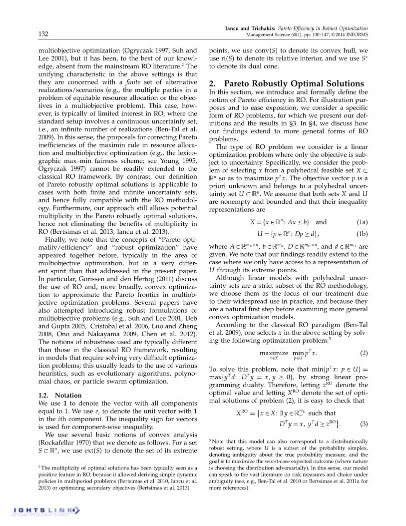
Example 3 (Nonconvexity of X

PRO). Consider the

following feasible set X and uncertainty set U :

X=8x2✓4+2 x111 x2+x361 x3+x451 x2+x4591

U =conv48ei

1 i2811000149950It can be checked that z

RO = 1, and X

RO = 8x 2 X2

x � 19. Also, x1 = 61 2 4 17T and x

2 = 61 4 2 17T areboth PRO solutions (they are the optimal solutionsto the problems of maximizing 6Ö Ö 1É 3Ö Ö7

T

and 6Ö 1É 3Ö Ö Ö7

T over XRO, respectively, for somesmall Ö > 0). However, the point 005x1 + 005x2 =61 3 3 17T y X

PRO, since it is Pareto dominated by61 3 3 27T 2X

RO.

The nonconvex structure of XPRO suggests that solv-ing optimization problems over the set may be com-putationally challenging in general. One particularcase when this is simple is when X

RO = X

PRO, whichcan be tested using the LP in Corollary 2. When X

RO 6=X

PRO, the following result provides some intuitionabout the structure of the latter set.

6 Note that in the classical RO framework, optimizing a linearsecondary objective over X

RO can be cast as an LP, utilizing thepolyhedral description of XRO in (3).

Dow

nloa

ded

from

info

rms.o

rg b

y [1

71.6

6.19

.162

] on

12 N

ovem

ber 2

014,

at 1

0:19

. Fo

r per

sona

l use

onl

y, a

ll rig

hts r

eser

ved.

Iancu and Trichakis: Pareto Efficiency in Robust Optimization138 Management Science 60(1), pp. 130–147, © 2014 INFORMS

Proposition 2. If XRO 6= X

PRO, then X

PRO \ ri4XRO5

=ô.

Proof of Proposition 2. We first argue that ifX

RO 6=X

PRO, then there does not exist a p 2 ri4U 5 suchthat pT x is constant for all x 2 X

RO. To see this, notethat if such a p existed, then the optimal objectivefunction in problem (7), for any point x 2X

RO, wouldhave to be zero, implying that XRO =X

PRO.Assume now that X

PRO \ ri4XRO5 6= ô, and con-

sider any x in the intersection. By Proposition 1, theremust exist p 2 ri4U 5 such that x 2 argmax

x2XRO pT

x.Furthermore, since pT x is not constant over XRO, theremust exist a y 2 X

RO such that p

T

y < p

T

x. But then,since x 2 ri4XRO

5, there exists a small enough Ö > 0such that x

def= x + Ö · 4x É y5 2 X

RO, for which p

T

x >

p

T

x—a contradiction. ÉThe previous result shows that the set XPRO is either

identical to X

RO or contained in the boundary of thelatter. This result is somewhat encouraging, since itmay allow a characterization of the convex hull ofX

PRO in particular cases. We do not pursue this ideafurther in the present paper.In a different sense, the results in Proposition 2

also suggest that whether a solution x 2 X

RO is actu-ally PRO critically depends on the algorithm usedfor solving the nominal RO problem. In particular, ifX

RO 6= X

PRO and the nominal RO problem is solvedusing a typical interior point method (i.e., one thatreturns solutions in the interior of the optimal face;see Ye 1992), then, by Proposition 2, the resulting solu-tion x 2 X

RO will not be PRO. However, even whenthe simplex method is used, there is still no reasonto a priori expect that the obtained solution would bePRO (see Example 2 of §2).We now return to the main question of interest,

i.e., developing a tractable procedure for optimiz-ing a linear objective over the set X

PRO, and wepresent two different approaches for addressing it.The first involves solving a mixed-integer linear pro-gram (MILP) and is summarized in the followingproposition.

Proposition 3. For any r 2✓n and any p 2 ri4U 5, let4x

?

1å

?

1á

?

1z

?

5 2 ✓n ⇥ ✓m

X ⇥ ✓⇥ 80119mX be an optimalsolution of the following MILP:

maximizex1å1á1z

r

T

x (10a)

subject to x 2X

RO1 (10b)

åM41É z51 (10c)

bÉAxMz1 (10d)

DA

T

åÉ dá�Dp1 (10e)

å� 01 á� 01 z 2 80119mX

1 (10f)

where M is a sufficiently large value. Then, x? is an opti-mal solution of the problem

maximizex2XPRO

r

T

x0

Proof of Proposition 3. We need to show that x 2X

RO is PRO if and only if there exist å 2 ✓m

X , á 2 ✓,and z 2 80119mX that satisfy (10c)–(10f).Fix a solution x 2 X

RO. By Theorem 1, x is PROif and only if, for an arbitrarily chosen p 2 ri4U 5,the optimal value in the problem maximize

y

8p

T

y2 y 2U

⇤1 x + y 2 X9 is zero. Equivalently, x is PRO if and

only if the optimal value in the following primal-dualLP pair is zero:

maximizeã

p

T

D

T

ã

subject to

d

T

ã�0AD

T

ãbÉAx

ã�0

=

minimizeå1á

å

T

4bÉAx5

subject to

DA

T

åÉdá�Dp

å�0á�00

To arrive at the primal (maximization), we used thedescription in (1a) for the set X, the expression in (8)for the dual cone U

⇤, and we eliminated the auxiliaryvariables y. Note that the primal is trivially feasible,with the choice ã = 0 resulting in an objective valueof zero. As such, whenever its optimal value is lessthan or equal to zero, strong LP duality must hold.We then have that the optimal value is zero if and

only if there exist å 2 ✓m

X and á 2 ✓ satisfying theconstraints of the dual, such that åT

4bÉAx5= 0. Thisis a bilinear constraint in variables x and å. In fact,since å � 0 and b É Ax � 01 8x 2 X

RO, it is equiva-lent to the linear complementarity constraints å

i

· 4bÉAx5

i

= 01 i = 11 0 0 0 1mX

(Luo et al. 1996). The latterconstraint can be modeled using variables z 2 80119mX

and constraints (10c) and (10d), where M is suffi-ciently large.7 ÉThe above approach should be very relevant in

practice, since large-scale MILPs can be solved in amatter of seconds using commercially available soft-ware such as CPLEX or Gurobi. In case this is stillan onerous task, one can also resort to the follow-ing simple heuristic for optimizing linear functionsover X

PRO: solve the problem maxx2XRO p

T

x for (sev-eral) randomly sampled points p 2 ri4U 5, collect allthe optimal solutions in a set XPRO, and then solve theproblem max

x2XPRO rT

x.Because, by Corollary 1 and Proposition 1 all the

PRO solutions can be generated by sampling points

7 Note that we need M � maxi=110001m

X

max4åi

1 maxx2X e

T

i

4b É Ax55.The latter term can always be bounded since X is compact. The for-mer term may also be bounded, depending on the dual feasible set.In practice, one may simply choose an increasing sequence of M ,stopping when the constraints for åM are no longer binding.

Dow

nloa

ded

from

info

rms.o

rg b

y [1

71.6

6.19

.162

] on

12 N

ovem

ber 2

014,

at 1

0:19

. Fo

r per

sona

l use

onl

y, a

ll rig

hts r

eser

ved.

Iancu and Trichakis: Pareto Efficiency in Robust OptimizationManagement Science 60(1), pp. 130–147, © 2014 INFORMS 139

p from the relative interior of U , the set X

PRO willbe a subset of the true X

PRO, so that this algorithmwill always produce a lower bound to the true opti-mal value. However, coupled with a suitable upperbound (e.g., obtained by maximizing r

T

x over X

RO),the heuristic may prove satisfactory in cases wherethe exact MILP in Proposition 3 is difficult to solve.

4. GeneralizationsIn this section, we discuss several directions forextending our earlier framework and results.

4.1. Uncertainty in the ConstraintsConsider a linear optimization problem where thecoefficients of the constraints matrix are uncertain.Specifically, consider the following RO formulation:

minimize c

T

x

subject to Ax� b1 8A 2U

A

1

(11)

where c 2 ✓n and b 2 ✓m are given, and U

A

⇢ ✓m⇥n

is a bounded polyhedral uncertainty set of the formtypically considered in the RO literature8 (Ben-Talet al. 2009). Problems with uncertainty in the vec-tors c and b can be readily reformulated so as tohave the same form as problem (11). For instance, incase c is uncertain, one can consider an equivalentepigraph formulation where the objective is replacedby an additional variable t and the extra constrainttÉ c

T

x� 0 is added.Let XRO be the optimal set and let zRO be the opti-

mal value of problem (11). The vector of slacks forconstraints in (11) for a solution x and uncertaintyrealization A, denoted by s4x1A5, is equal to

s4x1A5

def=AxÉ b1 8x 2✓n

1 A 2U

A

0

In view of the above, one can express XRO as follows:

X

RO = �x 2✓n

2 c

T

x z

RO1 s4x1A5� 01 8A 2U

A

0 (12)

A compact polyhedral description of X

RO is readilyavailable whenever such a description is also avail-able for U

A

, which we have assumed to be the casehere.According to classical RO, a robustly optimal solu-

tion x 2 X

RO in this setting protects us from worst-case realizations of A 2U

A

by ensuring that the slacksare nonnegative. Moreover, it does so at a minimum

8 The typical modeling assumption is that the matrix A dependsaffinely on a collection of primitive uncertain quantities, i.e., A4é5=P

m

i=1Ai

é

i

, where A

i

2✓m⇥n are known and é 2✓m denotes the prim-itive uncertain parameters, assumed to lie in an uncertainty set Ê⇢✓m. As such, whenever Ê has a compact polyhedral representation,the corresponding set U

A

= 8A4é52 é 2Ê9 does as well (see Ben-Talet al. 2009 for details).

cost c

T

x = z

RO. That is, by selecting a robustly opti-mal solution, we are guaranteed that no other solu-tion exists that yields nonnegative slacks under alluncertainty scenarios and at a lower cost than z

RO.However, in a similar spirit to our discussion in §2,such a selection criterion does not “optimize slacks”under all possible uncertain realizations—in fact, itfails to guarantee that no other solution exists yield-ing “larger” slacks and at the same cost as z

RO.The above observation gives rise to the notion of

PRO solutions for formulation (11). To evaluate theslacks provided by different solutions and uncertaintyrealizations, we introduce a slack value vector v 2 ✓m

that quantifies the relative value of slack in each con-straint.9 In particular, the slacks provided by solutionx, under scenario A, are valued at

v

T

s4x1A5= v

T

4AxÉ b51 8x 2✓n

1 A 2U

A

0

We have the following definition.

Definition 2. A solution x is called a PRO solutionfor problem (11) if it is robustly optimal, i.e., x 2X

RO,and there is no other x 2X

RO such that

v

T

s4x1A5� v

T

s4x1A51 8A 2U

A

1 and

v

T

s4x1 A5>v

T

s4x1 A51 for some A 2U

A

0

Similar to our discussion in §2, in this settingPRO solutions guarantee that slacks are optimizedfor all uncertainty realizations A 2 U

A

. Comparedwith robustly optimal solutions, PRO solutions havethe same qualities, i.e., they ensure feasibility at thelowest cost possible, but, in addition, they also pro-vide potentially higher slacks (as valued through vec-tor v). This is particularly important for the followingreasons:a. In the majority of problems of the form (11)

that are derived from practical applications, one ofthe constraints typically involves the actual realizedcost, e.g., because of an epigraph reformulation.10 Assuch, slack in that particular constraint immediatelytranslates into lower actual realized cost. We referthe reader to our numerical studies in §§5.2–5.3 forexamples.

9 We choose to compare two slack vectors by scalarization throughthe value vector v 2 ✓n, a method that is common in multiobjec-tive optimization (Boyd and Vandenberghe 2004). However, othermultidimensional orderings may be more suitable in particular set-tings (for instance, the Lorenz order). Extending our framework tosuch cases is an interesting direction that we do not pursue in thepresent paper.10 Note that an epigraph reformulation is necessary not only incases where the actual cost vector is uncertain (as discussed above),but also when the cost of the problem is piecewise affine; see, forinstance, Bertsimas et al. (2010).

Dow

nloa

ded

from

info

rms.o

rg b

y [1

71.6

6.19

.162

] on

12 N

ovem

ber 2

014,

at 1

0:19

. Fo

r per

sona

l use

onl

y, a

ll rig

hts r

eser

ved.

Iancu and Trichakis: Pareto Efficiency in Robust Optimization140 Management Science 60(1), pp. 130–147, © 2014 INFORMS

b. Solutions that provide zero or low values ofslack can more readily generate infeasibility as aresult of potential misspecifications of other modelparameters. For the value of slack, we refer the reader,for instance, to Joshi and Boyd (2009).Hence, similar to the notion studied in §2, PRO solu-tions in this setting have no downside and have con-siderable potential upside.From a methodological standpoint, the conditions

of Pareto domination in Definition 2 are equivalent to

4A

T

v5

T

x� 4A

T

v5

T

x1 8A 2U

A

1 and

4A

T

v5

T

x > 4A

T

v5

T

x1 for some A 2U

A

0

If we let p def=A

T

v and

U

def= 8A

T

v2 A 2U

A

91 (13)

we arrive at the same formulation of Pareto effi-ciency as in Definition 1. Using this observation, onecan extend all our findings in §3.1. For instance, theextended Corollary 1 would state the following.

Corollary 3. Consider an arbitrary point p 2 ri4U 5,where U is given by (13). Then, all the optimal solutions tomaximize

x2XRO pT

x are PRO for problem (11), where XRO

is given by (12).

As such, all the remarks in §3.1 pertaining toour results and their practical relevance hold in thepresent setting as well.

4.2. Mixed-Integer Linear Optimization ModelsA second direction for extending our results is thecase when some of the decisions x are constrainedto be integers. This is of great relevance in prac-tical applications, since many models of real-worldprocesses involve integrality constraints (see, e.g.,Bertsimas and Sim 2003).To this end, the present section is concerned with

the following problem:

maximizex2X

minp2U

p

T

x

X = �x 2✓n

2 Ax b1 x

i

2⇢1 8 i 2I 1

U = �p 2✓n

2 Dp� d

1

where I ✓ 811 0 0 0 1n9 is a set of indices, and A, b, D,and d are known.Our goal is to revisit the main results of §3 and

investigate their validity in the present setting. As ageneral overview, all the critical results can be suit-ably adapted to the new model: by solving particu-lar MILPs, one can (a) test whether a given x is aPRO solution (and, if not, obtain a PRO solution x

that Pareto dominates it), (b) generate PRO solutions,and (c) optimize linear objectives over the set of PRO

solutions. The sole results of §3 that no longer holdhere are Propositions 1 and 2—in particular, not allPRO solutions can be recovered by maximizing linearobjectives of the form p

T

x where p 2 ri4U 5, and the setX

PRO is not necessarily in the boundary of XRO whenthe two are different. For reasons of brevity, we refrainfrom reproving the (new) claims, since the argumentsexactly parallel their counterparts in §3.First, note that the representation for the set of

robust optimal solutions X

RO remains identical toexpression (3); i.e.,

X

RO=�x2X2 9y2✓m

U+ such that DT

y=x1 y

T

d�z

RO 0

Here, however, the optimal (worst-case) value forthe problem, z

RO, is obtained by solving an MILP(Bertsimas and Sim 2003), and the set X

RO also in-cludes integrality constraints due to X.In this context, we can reaffirm our first main result

in Theorem 1, which holds true without any modifi-cations. In particular, to test whether a point x 2X

RO

is also a PRO, one only needs to solve the optimiza-tion problem (7) for an arbitrarily chosen p in ri4U 5.As before, if the optimal value is exactly zero, then x 2X

PRO. Otherwise (i.e., strictly positive optimal value),x+y

? 2X

PRO, and it Pareto dominates x. We note thatthe sole change from the result in §3.1 is that prob-lem (7) is now an MILP instead of an LP. In particu-lar, the computational complexity for finding a PROsolution compared to just finding a solution x 2 X

RO

is still the same, because both now require solvingMILPs. However, the exact computational cost for theformer problem may be increased not only because ofthe requirement of solving additional MILPs but alsobecause it may not preserve some of the structure ofthe nominal MILP problem.As before, this theorem readily leads to a sim-

ple procedure for finding points x 2 X

PRO. In par-ticular, a result analogous to Corollary 1 holds: forany p 2 ri4U 5, all the optimal solutions to the MILPmaximize

x2XRO pT

x are guaranteed to be PRO points.Furthermore, just as stated in Corollary 2, determin-ing whether XRO =X

PRO resumes to solving the MILPin (9) and comparing the optimal value with zero.This result also brings us to the first main point of

departure from §3. Recall that by choosing differentpoints p 2 ri4U 5, the union of the sets argmax

x2XRO pT

x

was guaranteed to contain all PRO solutions for thecase without integrality constraints (see Proposition 1in §3.1). Unfortunately, that is no longer the case here.In particular, there may be points x 2X

PRO that lie inthe strict interior of the set conv4XRO

5 and hence can-not be recovered by maximizing a linear functionalover X

RO. The following example presents such aninstance.

Example 4 (Strictly Interior Point in X

RO). Let

X = 84x11x21x35 2 ⇢2+ ⇥ ✓2 1

2x1 + 15x2 11 x3 � É11

Dow

nloa

ded

from

info

rms.o

rg b

y [1

71.6

6.19

.162

] on

12 N

ovem

ber 2

014,

at 1

0:19

. Fo

r per

sona

l use

onl

y, a

ll rig

hts r

eser

ved.

Iancu and Trichakis: Pareto Efficiency in Robust OptimizationManagement Science 60(1), pp. 130–147, © 2014 INFORMS 141

Figure 2 Illustration of Sets and Points Considered in Example 4

PRO points

1

1

2

2

3

4

5

x1

x3

x2

conv(XRO)

Notes. The marked points correspond to all the points of X RO; PRO pointsare marked as stars. Note that one of the PRO points lies in the relativeinterior of the convex hull of X RO, which is shaded in gray.

x3 09, and let U = conv48e11 e21 e395. It can bechecked that

X

RO = 8x 2X2 x3 = 091

X

PRO = �60 2 07T 1 65 0 07T 1 61 2 07T

0

In particular, x = 61 2 07T 2 ri4conv4XRO55, and

therefore there is no p 2 ri4U 5 such that x 2argmax

x2XRO pT

x. Figure 2 provides a graphical illus-tration of XRO and X

PRO in this case.

Example 4 also proves that there are cases in whichX

RO 6= X

PRO and some points in X

PRO lie in the strict(relative) interior of XRO such that Proposition 2 alsodoes not hold.For the same reason, the sampling heuristic sug-

gested in §3.2 for optimizing a linear functional overX

PRO may not be very effective: one can certainly stillapply it, but since sampling points p 2 ri4U 5 is nolonger guaranteed to generate all the points in X

PRO,one may be unable to recover the exact (true) optimalvalue.However, we note that the problem of optimizing

linear objectives over X

PRO can nonetheless be dealtwith in a scalable fashion. In particular, the mainresult in Proposition 3 still holds, and, for any r 2✓n,the optimal value in the problem maximize

x2XPRO rT

x

can be obtained by solving the MILP in (10). As aresult, optimizing over XPRO when some decisions areintegral is as easy as finding a single x 2X

RO, unlikethe setting discussed in §3.2.

5. Numerical StudiesIn this section, we evaluate the implications of ourfindings by performing numerical studies. We focus

on three application areas in which RO has provento be very powerful. In particular, we study threeclassical problems from the literature drawn fromfinance, inventory management, and project manage-ment applications.We generate multiple instances of the problems we

consider, using random data, with the purpose ofassessing(a) the frequency at which computed robustly opti-

mal solutions are Pareto dominated by other solu-tions, and(b) the performance gain by considering PRO solu-

tions in practice instead of dominated robustly opti-mal solutions.For every generated instance, we solve an equivalentproblem to problem (9) using the simplex methodto identify dominated robustly optimal solutions andassociated PRO solutions.We find that in approximately 805% of the instances

we generate (across all three problems), there existrobustly optimal solutions that are Pareto dominatedby other PRO solutions. Moreover, using the associ-ated PRO solutions in these cases yields a relative per-formance gain that can be as high as 43% comparedwith using the dominated robustly optimal solutions.

5.1. Portfolio OptimizationRO has been widely studied and used in financial ser-vices applications, particularly in portfolio optimiza-tion problems. We refer the reader to Ben-Tal et al.(2000), Goldfarb and Iyengar (2003), Bertsimas andPachamanova (2008), Natarajan et al. (2008), Calafiore(2007), Ben-Tal et al. (2010), Gabrel et al. (2012) andthe book by Fabozzi et al. (2007) for a thoroughoverview.In this section, we consider a simple portfolio selec-

tion problem that has the form we studied in §2, i.e.,a linear program with uncertainty in the objective.

5.1.1. Problem Description. A manager wishes toinvest her wealth in n+1 investment opportunities orassets. We denote the return of the ith asset with r

i

,i = 11 0 0 0 1n + 1. The 4n + 15th asset yields a known,deterministic return of å

n+1, i.e.,

r

n+1 =å

n+11

with no associated risk. On the contrary, all remain-ing assets are risky. In particular, the return of the ithasset is equal to

r

i

=å

i

+ë

i

Ü

i

1 i= 11 0 0 0 1n1

where å

i

is the expected return of the ith asset; Üi

is arandom, uncertain shock affecting the return of the ithasset; and ë

i

is a volatility parameter. The values ofthe shocks Ü 2✓n are assumed to be bounded between

Dow

nloa

ded

from

info

rms.o

rg b

y [1

71.6

6.19

.162

] on

12 N

ovem

ber 2

014,

at 1

0:19

. Fo

r per

sona

l use

onl

y, a

ll rig

hts r

eser

ved.

Iancu and Trichakis: Pareto Efficiency in Robust Optimization142 Management Science 60(1), pp. 130–147, © 2014 INFORMS

É1 and 1, and they are assumed to sum up to zero.Uncertainty sets of this style have been introducedand used in Bandi and Bertsimas (2012).Let x 2 ✓n+1 be the target portfolio composition

vector; i.e., x

i

is the fraction of the wealth thatthe manager wishes to invest in the ith asset. Werequire that (a) no shorting is allowed, i.e., x � 0;and that (b) the net fraction of the wealth invested inany of the asset groups 811 0 0 0 1N/49, 8N/41 0 0 0 1N/29,8N/21 0 0 0 13N/49, and 83N/41 0 0 0 1N 9 does not exceed25%, for diversification purposes. The objective of themanager is to select a portfolio composition so as tomaximize its worst-case return.A formulation of the above RO problem is as

follows:

maximize minÜ2U

n+1X

i=1

r

i

x

i

subject to r

i

=å

i

+ë

i

Ü

i

1 i= 11 0 0 0 1n1

r

n+1 =å

n+11

44k+15N 5/4X

i=1+4kN 5/4

x

i

00251 k= 01112131

1T x= 11

x� 01

with variables r 2 ✓n+1, x 2 ✓n+1, and U = 8Ü 2 ✓n

2

É1 Ü 11 1T Ü = 09.

5.1.2. Data. We consider 10,000 instances of prob-lems of size n= 8. The expected returns of the riskyassets 8å

i

9

n

i=1 are independently sampled from a uni-formly distributed random variable taking values 1%,102%1 0 0 0 13%. The volatility parameters are set to ë

i

=002å

i

+ 008éi

, for all i = 11 0 0 0 1n, where the values8é

i

9

n

i=1 are independently sampled from the same ran-dom variable as the expected returns. The risk-freereturn is set to å

n+1 = 1%.

5.1.3. Results. The average number of instancesin which the solver found a robustly optimal solu-tion x that was not PRO was 31%. For these instances,we obtained a single PRO solution x by solving prob-lem (7), for which we recorded two different perfor-mance gaps. The first corresponded to the relativeimprovement that x yielded in objective comparedwith x if a “nominal” scenario p materialized, i.e.,

p

T

4xÉ x5

p

T

x

1

where p corresponds to Ü = 0 and the returns equal totheir expected values. The second gap correspondedto the maximum relative improvement across all pos-sible scenario realizations, i.e.,

maxp2U

p

T

4xÉ x5

p

T

x

0

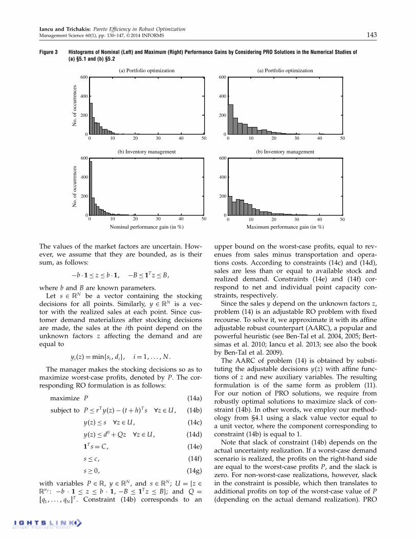
Histograms for both gaps are recorded in Figure 3(a).For the performance gaps under the nominal scenario,the median value recorded was 205%, whereas themaximum was as high as 22%. For the maximum per-formance gaps across all scenarios, the median valuerecorded was 5%, whereas the maximum was as highas 43%.

5.2. Inventory ManagementA different stream of applications in which RO hasproven particularly useful has been inventory andsupply chain management. For a thorough reviewand many references, we direct the interested readerto the papers by Ben-Tal et al. (2005), Bertsimas andThiele (2006), Adida and Perakis (2006), Bienstock andÖzbay (2008), Bertsimas et al. (2010, 2011b), and Seeand Sim (2010); the review papers by Bertsimas et al.(2011a) and Gabrel et al. (2012); and the book byBen-Tal et al. (2009).In this section, we consider a single-warehouse

multiple-retailer setting, where the manager needsto make stocking decisions in the face of uncertaindemand. From an RO perspective, the resulting prob-lem is a two-stage adjustable problem with fixedrecourse.

5.2.1. Problem Description. Consider a retail net-work consisting of a single warehouse and N differentretail points, indexed by i= 11 0 0 0 1N , where customerdemand is realized. For simplicity, we consider thecase where a single item is offered for sale.We have C units of the item available in the ware-

house that need to be distributed to the retail points.The ith retail point holds zero initial inventory and iscapable of stocking at most c

i

units. The transporta-tion costs for distributing or, equivalently, stocking,inventory at the ith retail point is t

i

currency unitsper unit of inventory. Similarly, we assume that thereis an operating cost at the ith retail point equal to h

i

currency units per unit of inventory.11 The revenuesfrom sales at the ith retail point are r

i

currency unitsper unit of inventory sold.Customer demand at each point is uncertain and

is driven by n

f

factors that affect the market. In par-ticular, we assume that the demand at the ith point,denoted by d

i

, is equal to

d

i

= d

0i

+ q

T

i

z1 i= 11 0 0 0 1N 1

where d

0i

is the nominal expected demand, z 2 ✓n

f isa vector of the realized values of the n

f

factors, andq

i

2✓n

f is a vector of parameters that measure theexposure of demand d

i

to each of the market factors.

11 For simplicity, we assume no fixed transportation or operat-ing costs, although one could include them in a straightforwardmanner.

Dow

nloa

ded

from

info

rms.o

rg b

y [1

71.6

6.19

.162

] on

12 N

ovem

ber 2

014,

at 1

0:19

. Fo

r per

sona

l use

onl

y, a

ll rig

hts r

eser

ved.

Iancu and Trichakis: Pareto Efficiency in Robust OptimizationManagement Science 60(1), pp. 130–147, © 2014 INFORMS 143

Figure 3 Histograms of Nominal (Left) and Maximum (Right) Performance Gains by Considering PRO Solutions in the Numerical Studies of(a) §5.1 and (b) §5.2

No.

of o

ccur

renc

esN

o. o

f occ

urre

nces

Nominal performance gain (in %) Maximum performance gain (in %)

00

00

00

0

2020

2020

4040

4040

1010

1010

3030

3030

5050

5050

200200

200

400400

400

600600

600

0

200

400

600(a) Portfolio optimization (a) Portfolio optimization

(b) Inventory management (b) Inventory management

The values of the market factors are uncertain. How-ever, we assume that they are bounded, as is theirsum, as follows:

Éb · 1 z b · 11 ÉB 1T z B1

where b and B are known parameters.Let s 2 ✓N be a vector containing the stocking

decisions for all points. Similarly, y 2 ✓N is a vec-tor with the realized sales at each point. Since cus-tomer demand materializes after stocking decisionsare made, the sales at the ith point depend on theunknown factors z affecting the demand and areequal to

y

i

4z5=min8si

1d

i

91 i= 11 0 0 0 1N 0

The manager makes the stocking decisions so as tomaximize worst-case profits, denoted by P . The cor-responding RO formulation is as follows:

maximize P (14a)

subject to P r

T

y4z5É 4t+h5

T

s 8z 2U 1 (14b)

y4z5 s 8z 2U 1 (14c)

y4z5 d

0 +Qz 8z 2U 1 (14d)

1T s =C1 (14e)

s c1 (14f)

s � 01 (14g)

with variables P 2 ✓, y 2 ✓N , and s 2 ✓N ; U = 8z 2✓n

f

2 Éb · 1 z b · 11 ÉB 1T z B9; and Q =6q11 0 0 0 1 qN 7

T . Constraint (14b) corresponds to an

upper bound on the worst-case profits, equal to rev-enues from sales minus transportation and opera-tions costs. According to constraints (14c) and (14d),sales are less than or equal to available stock andrealized demand. Constraints (14e) and (14f) cor-respond to net and individual point capacity con-straints, respectively.Since the sales y depend on the unknown factors z,

problem (14) is an adjustable RO problem with fixedrecourse. To solve it, we approximate it with its affineadjustable robust counterpart (AARC), a popular andpowerful heuristic (see Ben-Tal et al. 2004, 2005; Bert-simas et al. 2010; Iancu et al. 2013; see also the bookby Ben-Tal et al. 2009).The AARC of problem (14) is obtained by substi-

tuting the adjustable decisions y4z5 with affine func-tions of z and new auxiliary variables. The resultingformulation is of the same form as problem (11).For our notion of PRO solutions, we require fromrobustly optimal solutions to maximize slack of con-straint (14b). In other words, we employ our method-ology from §4.1 using a slack value vector equal toa unit vector, where the component corresponding toconstraint (14b) is equal to 1.Note that slack of constraint (14b) depends on the

actual uncertainty realization. If a worst-case demandscenario is realized, the profits on the right-hand sideare equal to the worst-case profits P , and the slack iszero. For non-worst-case realizations, however, slackin the constraint is possible, which then translates toadditional profits on top of the worst-case value of P(depending on the actual demand realization). PRO

Dow

nloa

ded

from

info

rms.o

rg b

y [1

71.6

6.19

.162

] on

12 N

ovem

ber 2

014,

at 1

0:19

. Fo

r per

sona

l use

onl

y, a

ll rig

hts r

eser

ved.

Iancu and Trichakis: Pareto Efficiency in Robust Optimization144 Management Science 60(1), pp. 130–147, © 2014 INFORMS

solutions ensure “optimal performance” under anydemand realization by maximizing this slack, unlikerobustly optimal solutions that ignore it.

5.2.2. Data. We consider 10,000 instances of prob-lems of size N = 10. The available inventory is set toC = 21000 units. All other problem data are indepen-dently sampled from uniformly distributed randomvariables. Inventory capacities at individual pointsc 2✓N are drawn between 300 and 500. Transporta-tion t 2✓N and operations cost rates h 2✓N are drawnbetween 1 and 3. Sales revenue rates r 2✓N are drawnbetween 20 and 40.Nominal demand values d

0 2 ✓N are drawn be-tween 100 and 200. The number of market factors n

f

is drawn from the values 2, 3, and 4. Exposure param-eters Q 2✓N⇥n

f are drawn between É2 and 2. Param-eters b and B that bound the factor values are set to 5and 25, respectively.

5.2.3. Results. The average number of instancesin which a robustly optimal solution was identifiedthat was not a PRO solution was 12%. For theseinstances, similarly with the study above, we com-puted the nominal and maximum performance gaps(in terms of actual profits) between the PRO solu-tion and the dominated robustly optimal solution weobtained. In this setting, the nominal scenario cor-responds to the case of z= 0 and customer demandequal to its expected value. The median performancegap under the nominal scenario recorded was 105%,whereas the maximum was as high as 20%. Themedian of the maximum gaps recorded was 605%,whereas the absolute maximum was as high as 35%.Related histograms are depicted in Figure 3(b).

5.3. Project ManagementThe third application that we consider is focused onrobust models for project management. These havebeen studied in several papers, including Cohen et al.(2007), Goh et al. (2010), Adida and Joshi (2009), andWiesemann et al. (2012). Here, we consider a modeldiscussed in Ben-Tal et al. (2009), where a managerneeds to make resource allocation decisions in the faceof uncertain processing times. From a methodologi-cal standpoint, the resulting problem is a two-stageadjustable RO problem with fixed recourse.

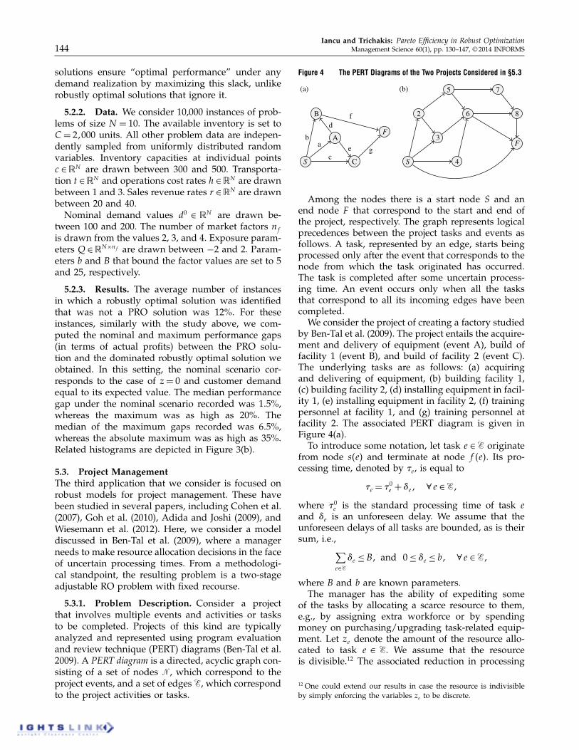
5.3.1. Problem Description. Consider a projectthat involves multiple events and activities or tasksto be completed. Projects of this kind are typicallyanalyzed and represented using program evaluationand review technique (PERT) diagrams (Ben-Tal et al.2009). A PERT diagram is a directed, acyclic graph con-sisting of a set of nodes N , which correspond to theproject events, and a set of edges E, which correspondto the project activities or tasks.

Figure 4 The PERT Diagrams of the Two Projects Considered in §5.3

S C

A

B

F

c

ab

d

e g

f

S 4

3

2

5

6

7

8

F

(a) (b)

Among the nodes there is a start node S and anend node F that correspond to the start and end ofthe project, respectively. The graph represents logicalprecedences between the project tasks and events asfollows. A task, represented by an edge, starts beingprocessed only after the event that corresponds to thenode from which the task originated has occurred.The task is completed after some uncertain process-ing time. An event occurs only when all the tasksthat correspond to all its incoming edges have beencompleted.We consider the project of creating a factory studied

by Ben-Tal et al. (2009). The project entails the acquire-ment and delivery of equipment (event A), build offacility 1 (event B), and build of facility 2 (event C).The underlying tasks are as follows: (a) acquiringand delivering of equipment, (b) building facility 1,(c) building facility 2, (d) installing equipment in facil-ity 1, (e) installing equipment in facility 2, (f) trainingpersonnel at facility 1, and (g) training personnel atfacility 2. The associated PERT diagram is given inFigure 4(a).To introduce some notation, let task e 2E originate

from node s4e5 and terminate at node f 4e5. Its pro-cessing time, denoted by í

e

, is equal to

í

e

= í

0e

+ Ñ

e

1 8 e 2E1

where í

0e

is the standard processing time of task e

and Ñ

e

is an unforeseen delay. We assume that theunforeseen delays of all tasks are bounded, as is theirsum, i.e.,

X

e2EÑ

e

B1 and 0 Ñ

e

b1 8 e 2E1

where B and b are known parameters.The manager has the ability of expediting some

of the tasks by allocating a scarce resource to them,e.g., by assigning extra workforce or by spendingmoney on purchasing/upgrading task-related equip-ment. Let z

e

denote the amount of the resource allo-cated to task e 2 E. We assume that the resourceis divisible.12 The associated reduction in processing

12 One could extend our results in case the resource is indivisibleby simply enforcing the variables z

e

to be discrete.

Dow

nloa

ded

from

info

rms.o

rg b

y [1

71.6

6.19

.162

] on

12 N

ovem

ber 2

014,

at 1

0:19

. Fo

r per

sona

l use

onl

y, a

ll rig

hts r

eser

ved.

Iancu and Trichakis: Pareto Efficiency in Robust OptimizationManagement Science 60(1), pp. 130–147, © 2014 INFORMS 145

time of task e is then r z

e

, where r is the time reduc-tion rate per unit of resource allocated. The maxi-mum resource amount that can be allocated to anytask is equal to c, and the manager has C units of theresource that need to be allocated so as to minimizethe worst-case completion time T of the project.If we denote the time that event ç 2 N occurs

with t

ç

, it can be seen that tç

depends on the uncer-tain delays Ñ. More formally, if we let 6S7

def= ô andrecursively define 6v7

def=Se=4u1v52E86u7[ 8e99 as the set

of all edges on directed paths from S to v that precedenode v, then it can be readily seen that t

ç

dependson the delays on the edges in 6ç7, which we denoteby Ñ

6ç7

.The following formulation captures the manager’s

problem:

minimize T (15a)

subject to

t

F

4Ñ

6F 7

5 T 1 8Ñ 2U 1 (15b)

t

S

= 01 (15c)

t

f 4e5

4Ñ

6f 4e57

5É t

s4e5

4Ñ

6s4e57

5� í

0e

+ Ñ

e

É rz

e

1

8e 2E1 8Ñ 2U 1 (15d)

1T z=C1 (15e)

z c1 (15f)

z� 00 (15g)

Here, U = 8Ñ 2 ✓óEó2 0 Ñ b · 11 1T Ñ B9 is the

uncertainty set, T 2 ✓ and z 2 ✓óEó are nonadjustabledecisions,13 and the times t 2 ✓óN ó are adjustable,allowed to depend on the delays realized on edges.Constraints (15b) and (15c) determine the end andstart times of the project. Constraint (15d) enforceslogical precedence of tasks and events as discussedabove. Constraints (15e) and (15f) limit the amount ofthe resource to be allocated.Problem (15) is an adjustable RO problem with

fixed recourse. To solve it, we approximate it with itsAARC similarly to the inventory management prob-lem in the previous section.For our notion of PRO solutions, we require from

robustly optimal solutions to maximize slack of con-straint (15b), because it translates to potential reduc-tion of the worst-case value of T (depending on theactual delay realizations). That is, we again employour methodology from §4.1 using a slack value vectorequal to a unit vector, where the component corre-sponding to constraint (15b) is equal to 1.

13 In our model, we assume that the resource allocation decisions zmust be made far in advance, before observing the realized delays;in practice, one could also consider adjustable policies. See Ben-Talet al. (2009) or Wiesemann et al. (2012) for details.

We study separately two PERT graphs, depicted inFigure 4:(a) the topology from Ben-Tal et al. (2009) we have

discussed thus far (panel a), and(b) a more complicated, randomly generated topol-

ogy (panel b).

5.3.2. Data. We consider 10,000 instances for eachcase (a) and (b). The standard processing times í

0 2✓óEó are independently sampled from a uniformly dis-tributed random variable (a) between 1 and 10, and(b) between 5 and 20. Parameters B and b that boundthe unforeseen delays are set to 6 and 2 for case (a),respectively, and 25 and 5 for case (b). The processingtime reduction rate r is (a) 1 and (b) 5. The maximumallowable resource at each task c is set to 1 for (a).For case (b), we replace constraint (15f) with í

0e

�r z

e

8 e 2 E to ensure nonnegativity of task process-ing times. The resource amount available C is set to(a) 3 and (b) 10.

5.3.3. Results. The average percentage of in-stances in which a robustly optimal solution was iden-tified that was not a PRO solution was 305% for case (a)and 7% for case (b). Similar to the study above, forthese instances we computed the nominal and maxi-mum performance gaps (in terms of actual completiontime) between the PRO solution and the dominatedrobustly optimal solution we obtained. In this setting,the nominal scenario corresponds to the case whereÑ is the analytic center of U , and tasks are equallydelayed. The median performance gap under the nom-inal scenario recorded was (a) 205% and (b) 105%,whereas the maximum was as high as (a) 12% and(b) 15%. The median of the maximum performancegaps recorded was (a) 405% and (b) 10%, whereasthe absolute maximum was as high as (a) 25% and(b) 27%. Related histograms are depicted in Figure 5.

6. ConclusionsIn this paper, we adapted the well-known conceptof Pareto efficiency in the context of the popular ROmethodology. We argued that by focusing exclusivelyon worst-case outcomes, the classical RO paradigmneed not produce solutions that are also Paretooptimal, leading to inefficiencies and suboptimalperformance in practice. We provided a basic theoret-ical characterization of PRO solutions and extendedthe RO framework by proposing practical methodsthat verify Pareto optimality, and we generate solu-tions that are PRO. Critically important, our approachinvolves solving optimization problems that are of thesame complexity as the underlying robust problems;hence, the potential improvements come at essen-tially limited extra computational cost. Our numericalexperiments, drawn from three different applicationareas (portfolio optimization, inventory management,

Dow

nloa

ded

from

info

rms.o

rg b

y [1

71.6

6.19

.162

] on

12 N

ovem

ber 2

014,

at 1

0:19

. Fo

r per

sona

l use

onl

y, a

ll rig

hts r

eser

ved.

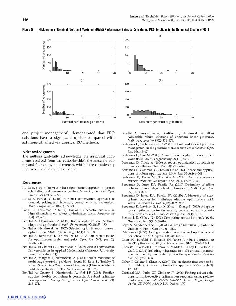
Iancu and Trichakis: Pareto Efficiency in Robust Optimization146 Management Science 60(1), pp. 130–147, © 2014 INFORMS

Figure 5 Histograms of Nominal (Left) and Maximum (Right) Performance Gains by Considering PRO Solutions in the Numerical Studies of §5.3

Num

ber o

f occ

urre

nces

Num

ber o

f occ

urre

nces

Nominal performance gain (in %) Maximum performance gain (in %)

00

00

0

2020 4040 1010 30

0 20 4010 30

30

0 20 4010 30

50

100100

100

150

200200

200

0

50

100

150

200

300300

400400

(a) (a)

(b) (b)

and project management), demonstrated that PROsolutions have a significant upside compared withsolutions obtained via classical RO methods.

AcknowledgmentsThe authors gratefully acknowledge the insightful com-ments received from the editor-in-chief, the associate edi-tor, and four anonymous referees, which have considerablyimproved the quality of the paper.

ReferencesAdida E, Joshi P (2009) A robust optimisation approach to project

scheduling and resource allocation. Internat. J. Services, Oper.Informatics 4(2):169–193.

Adida E, Perakis G (2006) A robust optimization approach todynamic pricing and inventory control with no backorders.Math. Programming 107(1):97–129.

Bandi C, Bertsimas D (2012) Tractable stochastic analysis inhigh dimensions via robust optimization. Math. Programming134(1):23–70.

Ben-Tal A, Nemirovski A (2002) Robust optimization—Method-ology and applications. Math. Programming 92(3):453–480.

Ben-Tal A, Nemirovski A (2007) Selected topics in robust convexoptimization. Math. Programming 112(1):125–158.

Ben-Tal A, Bertsimas D, Brown DB (2010) A soft robust modelfor optimization under ambiguity. Oper. Res. 58(4, part 2):1220–1234.

Ben-Tal A, El-Ghaoui L, Nemirovski A (2009) Robust Optimization,Princeton Series in Applied Mathematics (Princeton UniversityPress, Princeton, NJ).

Ben-Tal A, Margalit T, Nemirovski A (2000) Robust modeling ofmulti-stage portfolio problems. Frenk H, Roos K, Terlaky T,Zhang S, eds. High Performance Optimization (Kluwer AcademicPublishers, Dordrecht, The Netherlands), 303–328.

Ben-Tal A, Golany B, Nemirovski A, Vial J-P (2005) Retailer-supplier flexible commitments contracts: A robust optimiza-tion approach. Manufacturing Service Oper. Management 7(3):248–271.

Ben-Tal A, Goryashko A, Guslitzer E, Nemirovski A (2004)Adjustable robust solutions of uncertain linear programs.Math. Programming 99(2):351–376.

Bertsimas D, Pachamanova D (2008) Robust multiperiod portfoliomanagement in the presence of transaction costs. Comput. Oper.Res. 35(1):3–17.

Bertsimas D, Sim M (2003) Robust discrete optimization and net-work flows. Math. Programming 98(1–3):49–71.

Bertsimas D, Thiele A (2006) A robust optimization approach toinventory theory. Oper. Res. 54(1):150–168.

Bertsimas D, Caramanis C, Brown DB (2011a) Theory and applica-tions of robust optimization. SIAM Rev. 53(3):464–501.

Bertsimas D, Farias VF, Trichakis N (2012) On the efficiency-fairness trade-off. Management Sci. 58(12):2234–2250.

Bertsimas D, Iancu DA, Parrilo PA (2010) Optimality of affinepolicies in multistage robust optimization. Math. Oper. Res.35(2):363–394.

Bertsimas D, Iancu DA, Parrilo PA (2011b) A hierarchy of near-optimal policies for multistage adaptive optimization. IEEETrans. Automatic Control 56(12):2809–2824.

Bertsimas D, Litvinov E, Sun X, Zhao J, Zheng T (2013) Adaptiverobust optimization for the security constrained unit commit-ment problem. IEEE Trans. Power Systems 28(1):52–63.

Bienstock D, Özbay N (2008) Computing robust basestock levels.Discrete Optim. 5(2):389–414.

Boyd S, Vandenberghe L (2004) Convex Optimization (CambridgeUniversity Press, Cambridge, UK).

Calafiore G (2007) Ambiguous risk measures and optimal robustportfolios. SIAM J. Optim. 18(3):853–877.

Chan TC, Bortfeld T, Tsitsiklis JN (2006) A robust approach toIMRT optimization. Physics Medicine Biol. 51(10):2567–2583.

Chen W, Unkelbach J, Trofimov A, Madden T, Kooy H, Bortfeld T,Craft D (2012) Including robustness in multi-criteria optimiza-tion for intensity-modulated proton therapy. Physics MedicineBiol. 57(3):591–608.

Cohen I, Golany B, Shtub A (2007) The stochastic time-cost trade-off problem: A robust optimization approach. Networks 49(2):175–188.

Cristobal MA, Parks GT, Clarkson PJ (2006) Finding robust solu-tions to multi-objective optimisation problems using polyno-mial chaos. Proc. 6th ASMO UK/ISSMO Conf. Engrg. DesignOptim. CD-ROM. ASMO UK, Oxford, UK.

Dow

nloa

ded

from

info

rms.o

rg b

y [1

71.6

6.19

.162

] on

12 N

ovem

ber 2

014,

at 1

0:19

. Fo

r per

sona

l use

onl

y, a

ll rig

hts r

eser

ved.

Iancu and Trichakis: Pareto Efficiency in Robust OptimizationManagement Science 60(1), pp. 130–147, © 2014 INFORMS 147

Deb K, Gupta H (2005) Searching for robust Pareto-optimalsolutions in multi-objective optimization. Coello Coello CA,Hernández Aguirre A, Zitzler E, eds. Evolutionary Multi-Criterion Optimization, Lecture Notes in Computer Science,Vol. 3410 (Springer, Berlin), 150–164.

El-Ghaoui L, Oustry F, Lebret H (1998) Robust solutions to uncer-tain semidefinite programs. SIAM J. Optim. 9(1):33–52.

Fabozzi F, Kolm P, Pachamanova D, Focardi S (2007) Robust Portfo-lio Optimization and Management. Frank J. Fabozzi Series (JohnWiley & Sons, Hoboken, NJ).

Fischetti M, Monaci M (2009) Light robustness. Ahuja R,Möhring R, Zaroliagis C, eds. Robust and Online Large-ScaleOptimization, Lecture Notes in Computer Science, Vol. 5868(Springer, Berlin), 61–84.

Gabrel V, Murat C, Thiele A (2012) Recent advances in robustoptimization and robustness: An overview. Technical report,LAMSADE, Universite Paris-Dauphine, Paris.

Gabrel V, Murat C, Wu L (2013) New models for the robust shortestpath problem: Complexity, resolution and generalization. Ann.Oper. Res. 207(1):97–120.

Goh J, Hall N, Sim M (2010) Robust optimization strategies for totalcost control in project management. Working paper, StanfordUniversity, Stanford, CA.

Goldfarb D, Iyengar G (2003) Robust portfolio selection problems.Math. Oper. Res. 28(1):1–38.

Gorissen BL, den Hertog D (2011) Approximating the Paretoset of multiobjective linear programs via robust optimiza-tion. CentER Discussion Paper 2012-031, Center for EconomicResearch, Tilburg University, Tilburg, The Netherlands.

Iancu DA, Sharma M, Sviridenko M (2013) Supermodularity andaffine policies in dynamic robust optimization. Oper. Res.61(4):941–956.

Joshi S, Boyd S (2009) An efficient method for large-scale slackallocation. Engrg. Optim. 41(12):1163–1176.

Kalai R, Lamboray R, Vanderpooten D (2012) Lexicographic Å-robustness: An alternative to min–max criteria. Eur. J. Oper.Res. 220(3):722–728.

Leung JY-T, Pinedo M, Wan G (2010) Competitive two-agentscheduling and its applications. Oper. Res. 58(2):458–469.

Lim AEB, Shanthikumar JG (2007) Relative entropy, exponentialutility, and robust dynamic pricing. Oper. Res. 55(2):198–214.

Luo B, Zheng J (2008) A new methodology for searching robustPareto optimal solutions with MOEAs. Proc. IEEE WorldCongress Comput. Intelligence (IEEE, Piscataway, NJ), 580–586.

Luo Z-Q, Pang J-S, Ralph D (1996) Mathematical Programs with Equi-librium Constraints (Cambridge University Press, Cambridge,UK).

Natarajan K, Pachamanova D, Sim M (2008) Incorporating asym-metric distributional information in robust value-at-risk opti-mization. Management Sci. 54(3):573–585.

Ogryczak W (1997) On the lexicographic minimax approach tolocation problems. Eur. J. Oper. Res. 100(3):566–585.

Ono S, Nakayama S (2009) Multi-objective particle swarm opti-mization for robust optimization and its hybridization withgradient search. IEEE Congress Evolutionary Comput. (IEEE,Piscataway, NJ), 1629–1636.

Perakis G, Roels G (2010) Robust controls for network revenuemanagement. Manufacturing Service Oper. Management 12(1):56–76.

Rockafellar T (1970) Convex Analysis (Princeton University Press,Princeton, NJ).

Roy B (2010) Robustness in operational research and decision aid-ing: A multi-faceted issue. Eur. J. Oper. Res. 200(3):629–638.

Rusmevichientong P, Topaloglu H (2012) Robust assortment opti-mization in revenue management under the multinomial logitchoice model. Oper. Res. 60(4):865–882.

Savage LJ (1972) The Foundations of Statistics, 2nd ed. (Dover Pub-lications, Mineola, NY).

Schrijver A (2000) Theory of Linear and Integer Programming, 2nd ed.(John Wiley & Sons, Chichester, UK).

See C-T, Sim M (2010) Robust approximation to multiperiod inven-tory management. Oper. Res. 58(3):583–594.

Soyster AL (1973) Convex programming with set-inclusive con-straints and applications to inexact linear programming. Oper.Res. 21(5):1154–1157.

Sturm J, Polik I, Terlaky T (2006) SeDuMi 1.3. http://sedumi.ie.lehigh.edu/.

Suh M, Lee T (2001) Robust optimization method for the economicterm in chemical process design and planning. Indust. Engrg.Chemistry Res. 40(25):5950–5959.

Wiesemann W, Kuhn T, Rustem B (2012) Robust resource allo-cations in temporal networks. Math. Programming 135(1–2):437–471.

Ye Y (1992) On the finite convergence of interior-point algorithmsfor linear programming. Math. Programming 57(1–3):325–335.

Young HP (1995) Equity: In Theory and Practice (Princeton Univer-sity Press, Princeton, NJ).

Dow

nloa

ded

from

info

rms.o

rg b

y [1

71.6

6.19

.162

] on

12 N

ovem

ber 2

014,

at 1

0:19

. Fo

r per

sona

l use

onl

y, a

ll rig

hts r

eser

ved.