Embed Size (px)
Citation preview

IZA DP No. 2516
Parental Education and Child Health:Evidence from a Schooling Reform
Maarten LindeboomAna Llena-NozalBas van der Klaauw
DI
SC
US
SI
ON
PA
PE
R S
ER
IE
S
Forschungsinstitutzur Zukunft der ArbeitInstitute for the Studyof Labor
December 2006
Parental Education and Child Health: Evidence from a Schooling Reform
Maarten Lindeboom Free University Amsterdam,
Tinbergen Institute, HEB, Netspar and IZA Bonn
Ana Llena-Nozal Free University Amsterdam
and Tinbergen Institute
Bas van der Klaauw Free University Amsterdam,
Tinbergen Institute, CEPR and IZA Bonn
Discussion Paper No. 2516 December 2006
IZA
P.O. Box 7240 53072 Bonn
Germany
Phone: +49-228-3894-0 Fax: +49-228-3894-180
E-mail: [email protected]
Any opinions expressed here are those of the author(s) and not those of the institute. Research disseminated by IZA may include views on policy, but the institute itself takes no institutional policy positions. The Institute for the Study of Labor (IZA) in Bonn is a local and virtual international research center and a place of communication between science, politics and business. IZA is an independent nonprofit company supported by Deutsche Post World Net. The center is associated with the University of Bonn and offers a stimulating research environment through its research networks, research support, and visitors and doctoral programs. IZA engages in (i) original and internationally competitive research in all fields of labor economics, (ii) development of policy concepts, and (iii) dissemination of research results and concepts to the interested public. IZA Discussion Papers often represent preliminary work and are circulated to encourage discussion. Citation of such a paper should account for its provisional character. A revised version may be available directly from the author.

IZA Discussion Paper No. 2516 December 2006
ABSTRACT
Parental Education and Child Health: Evidence from a Schooling Reform
This paper investigates the impact of parental education on child health outcomes. To identify the causal effect we explore exogenous variation in parental education induced by a schooling reform in 1947, which raised the minimum school leaving age in the UK. Findings based on data from the National Child Development Study suggest that postponing the school leaving age by one year had little effect on the health of their offspring. Schooling did however improve economic opportunities by reducing financial difficulties among households. We conclude from this that the effects of parental income on child health are at most modest. JEL Classification: I12, I28 Keywords: returns to education, intergenerational mobility, health, regression-discontinuity Corresponding author: Bas van der Klaauw Department of Economics Free University Amsterdam De Boelelaan 1105 1081 HV Amsterdam The Netherlands E-mail: [email protected]

1
1 Introduction
Studies have found that poor infant health persists into adulthood and that poor infant health
contributes to the health income gradient found later in life (see Case, Fertig and Paxson, 2005;
and the references cited therein). It is therefore important to examine which factors determine
infant health and whether their effect is causal. In this paper we look at the effect of parental
education on child health.
There are different channels through which parental education can affect their children’s
health. Education might have a direct impact on child health because it increases the ability to
acquire and process information. This helps parents to make better health investments for
themselves and their children and may result in better parenting in general. Alternatively,
education can affect child health through indirect pathways. An increased level of education can
give access to more skilled work with higher earnings and these resources could be used to invest
in health and to cushion the impact of adverse health shocks (Case, Lubotsky and Paxson, 2002).
In the presence of assortative mating, individuals with a higher level of education also marry
partners with higher levels of education, which positively affect family income. Case, Lubotsky
and Paxson (2002) find that parents’ long run income is important for the child’s health.
Furthermore, attending school for a longer time could lead to a change in preferences by either
lowering the discount rate or increasing risk-aversion (Cutler and Lleras-Muney, 2006). Finally,
increased education can increase the opportunity cost of having children and change fertility
choices or delay having children. However, McCrary and Royer (2006) do not find any effect of
mother’s education on fertility choices.
While all these channels are potential explanations to why parental education might
induce better child health, parental education and child health can also be related in non-causal
ways. Indeed, endowments that are transmitted across generations can cause a positive
association between parental education and child health. To overcome such endogeneity problems
it is necessary to find some exogenous variation in parental education. Recently the use of
schooling reforms as a source of exogenous variation has become popular in labor and health
economics. Most studies focus on the causal impact of education on earnings (e.g. Harmon and
Walker, 1995; Meghir and Palme, 2005; Pischke and Von Wachter, 2005) or on the effect of
parental income on the education of their children (e.g. Black, Devereux and Salvanes, 2005;
Chevalier, Harmon, O’Sullivan and Walker, 2005; Holmlund, Lindahl and Plug, 2006;
Oreopoulos, Page and Stevens, 2006). Only a few papers have examined the impact of education
on health. Oreopoulos (2006) uses changes in the minimum school leaving ages in the UK and

2
Ireland and finds that an extra year of schooling increases earnings and improves self-assessed
health when leaving school. Lleras-Muney (2005) uses variation across states in compulsory
education laws and finds that an additional year of education lowers mortality. Using Danish
panel data, Arendt (2005) finds inconclusive results of education on self-reported health and body
mass index. He finds, however, that an increase in education reduces the probability that a person
smokes. Currie and Moretti (2003) examine the impact of college openings on women’s
educational attainment and their infants’ health. They find that maternal education does improve
their offspring’s health. Part of the effect is assigned to the increased use of prenatal care and
reduced smoking. McCrary and Royer (2006) exploit discontinuities in school entry policies in
California and Texas to assess the effect of education on fertility and infant health outcomes.
They find that education does not affect observable inputs to infant health and has only small
effects on infant health. Finally, Doyle, Harmon and Walker (2005) use a schooling reform and
grandparental smoking behavior to instrument parental education and income and find no effect
of parental income on the health of their offspring and weak effects of parental education. They
conclude from this that the significant effects of parental income on child health as found in Case,
Lubotsky and Paxson (2002) and Currie, Shields and Wheatley-Price (2006) is spurious.
In this paper, we use a schooling reform that took place in the United Kingdom in 1947.
The reform raised the minimum school leaving age from 14 to 15. We show that the reform only
affected the schooling decision of individuals at the lower end of the education distribution; the
fraction of individuals leaving school at age 16 or later remained unaffected by the reform. More
precisely, due to the reform about 50% of the individuals in a birth cohort raised their school
leaving age from 14 to 15. We focus our empirical analyses mainly on those parents (fathers and
mothers) leaving school at age 14 and 15.1 This means that the estimated impact of parental
education should be considered as local average treatment effects (see Imbens and Angrist, 1994).
We show that restricting the data increases the impact of the reform on schooling compared to
using individuals with all levels of schooling as is done in previous studies. Previous approaches
in this literature (e.g. Chevalier, Harmon, O’Sullivan and Walker, 2005; Doyle, Harmon and
Walker, 2005; Oreopoulos, 2006) mostly included all schooling levels in the analyses, thereby
implicetly assuming that reforms at the lower end of the education distribution also affect school
leaving ages of those at the higher end of the education distribution. In the absence of such effects
on the higher end of the education distribution this might lead to a weak instruments problem that
will bias the results.
1 This is in line with the approach taken by Black, Devereux and Salvanes (2005).

3
We assess the causal effect of parental education on a wide range of child health
variables. These variables include health measured at birth as well as health measured later in
childhood. We discussed above that parental education might affect child health through different
mechanisms. We therefore also examine whether parental education causally affects parental
behavior, parental health and labor market outcomes. We find little effect of a direct causal
relationship between parental education and child health. We also find that increased parental
education reduces possible financial difficulties in the family. We therefore conclude that the
effects of parental education and income on child health are at most modest.
The remainder of this paper is organized as follows. In Section 2 we describe the dataset,
and in Section 3 we discuss the background of the 1947 reform. Section 4 presents the empirical
specification. The results are presented in Section 5 and we close with a discussion and
conclusion in section 6.
2 Data
The National Child Development Study is a longitudinal study of about 17,000 babies born in
Great Britain in the week of 3-9 March 1958. The study started as the “Perinatal Mortality
Survey” and surveyed the economic and obstetric factors associated with stillbirth and infant
mortality. Since the first wave, cohort members have been traced on six other occasions to
monitor their physical, educational and social circumstances. The interviews were carried out in
1965 (age 7), 1969 (age 11), 1974 (age 16), 1981 (age 23), 1991 (age 33) and 1999 (age 42). For
the birth survey, information was gathered from the mother and medical records. For the surveys
during childhood and adolescence, interviews were carried out with parents, teachers, and the
school health service. The advantage of the National Child Development Study is that it contains
information on both parents and children about education, health and other background
characteristics.
The main indicators of health at birth are birth weight and an indicator for whether the
child experienced an illness in the first week of life. We exclude twins from our sample since
their birth weight is not comparable with singletons. Illnesses at birth can be: incompatible Rh,
severe jaundice, congenital malformation, convulsions (or cerebral irritation/cyanotic attacks),
hypothermia, respiratory distress, infection, and pyloric stenosis. During later years in childhood
and adolescence, parents are asked questions about their children’s record of illnesses,
psychological problems, accidents and hospitalizations. A medical examination is performed by a
physician who records the child’s specific medical problems. Using this information we develop

4
several measures of child health. The first one is a measure of morbidity based on the number of
conditions the child has experienced at ages 7, 11 and 16 (as reported by both parents and the
physician)2. In addition, the survey contains information on the height and weight of the cohort
members measured by a physician (and therefore less subject to measurement error than self-
reports), which can be used to construct anthropometric indicators. Height-for-age-z-scores are
built by comparing the height data with the distribution of height for a reference population,
which is constructed by the US National Center for Health Statistics. Low height for age, or
stunting, is an indicator of past growth failure and is associated with frequent or chronic illness,
chronic inappropriate nutrition (insufficient energy intake and protein), and poverty. Height and
weight are also used to construct the Body Mass Index, which is a measure for overweight and
thinness. We use the height-for-age-z-scores and the Body Mass Index when the child was 7, 11
and 16.
We know the year of birth of the parents and the age at which they left full-time
education. In each wave we have information on the mother’s working status and on whether the
family experienced financial difficulties. We choose not to use information on wages given the
low response rate for this variable. The National Child Development Study records parental
weight and height when the child is age 11. This information can be transformed to obtain the
Body Mass Index. In addition, chronic conditions for the father and/or mother are recorded in all
waves during childhood and adolescence. We use this information to construct a dummy for the
presence of chronic conditions. Both can be used as measures for parental health. Finally, we
have some information about fertility since the birth survey contains a measure of parity (the
number of times the mother has given birth in 1958) and on the number of siblings the cohort
member has at each age.
Table 1 shows sample statistics of parental and child variables for different levels of
parental education. For this study, we focus on the sample of cohort members who have both their
natural parents between 1965 and 1974. We observe that parents with more education have better
socioeconomic and health outcomes. In particular, both more educated fathers and mothers have
higher earnings and the prevalence of chronic conditions and obesity is lower among this group.
Furthermore, all measures of child health are better for higher educated parents (lower probability
of birth weight, illness at birth, serious conditions, stunting, and obesity). This shows the presence
of the positive association between parental socioeconomic status and health that is also found in
other studies.
2 The conditions are categorized under 12 groups (see Power and Peckham, 1987).

5
3 Background of he 1947 reform and changes in schooling distribution
3.1 Description of the education reform
The Education Act of 1944 changed the education system for secondary schools in England and
Wales. It introduced a tripartite system whereby secondary schools were divided into: grammar
schools (academic track), secondary technical and secondary modern schools. Students were
allocated on the basis of an exam known as the 11 plus. It also made secondary education free for
all. The aims of the education reform were to “improve the future efficiency of the labor force,
increase physical and mental adaptability, and prevent the mental and physical cramping caused
by exposing children to monotonous occupations at an especially impressionable age”
(Oreopoulos, 2006). In addition, the Act resulted in the raising of the minimum school-leaving
age from 14 to 15 in April 1947. According to Galindo-Rueda (2003), the reform brought about
an increase in the number of pupils that was largely concentrated among the secondary modern
and technical schools where there were few entry requirements based on ability.
3.2 Distribution of schooling before and after the reform in the National Child Development Study data
The National Child Development Study includes parents born at different dates who are therefore
affected differently by the reform. The first cohort of parents that is affected by the reform is born
in 1934; they had to stay in school until the age of 15, compared to 14 for previous cohorts.
Figure 1 shows the mean age of finishing school by year of birth for fathers and mothers. The
mean age experiences a sharp raise in 1934, showing that the reform raised schooling age by on
average 3 months for fathers and 4.5 months for mothers. Previous to the reform fathers’
education reached a peak in 1930 and started to decline while mother’s education declined later,
in 1932. This is due to the fact that fathers tend to be older than mothers in our sample (see
frequency of birth years in Table 2). In addition, after the original increase caused by the reform
we observe a decrease in the mean age of schooling. Note that these are parents who had a child
in 1958 and that less educated individuals are more likely to have children at young ages. This
can lead to a sample where older individuals are more likely to have more education.
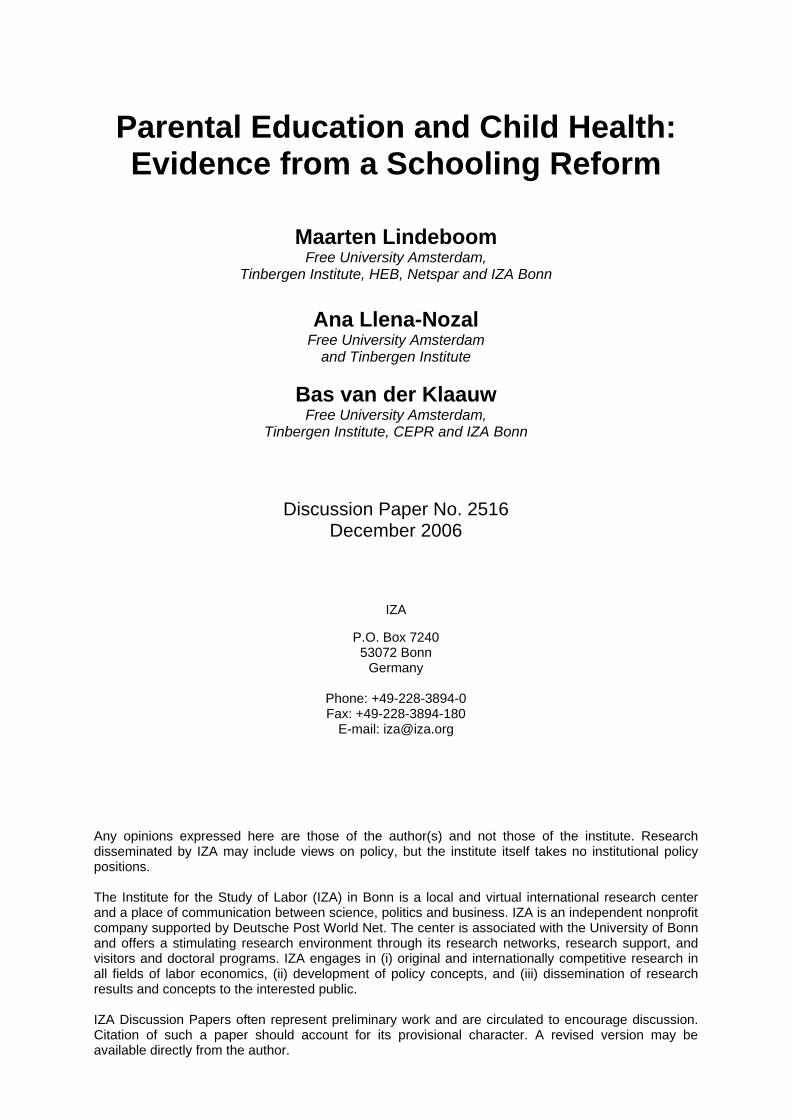
Figures 2 and 3 depict the percentages of parents leaving school at each age (stratified
according to their year of birth). We see that prior to the reform more than 60% of the population
left school at age 14 while between 10 and 20% (depending on the year and gender) left at age 15.
Within two years after the reform, close to 70% of fathers and mothers left at age 15. The graphs
show that the proportion leaving at age 16 and beyond remains similar before and after the

6
implementation of the new minimum school leaving age. It therefore appears that the reform
primarily affected those who would have left school earlier in absence of the reform. In 1934 only
about 50% finished school at age 15 (55% for mothers), while 20% of mothers and 30% of
fathers stayed until age 14 only. This is most likely due to partial implementation of the reform or
to pupils turning 14 before the reform was fully passed. Since we do not have the exact date of
birth we cannot check either hypothesis. Galindo-Rueda (2003) investigated whether behavioral
responses to the reform varied according to observable characteristics. He found that mothers
from smaller families and with skilled or semi-skilled parents were more likely to increase their
schooling (the response was not heterogeneous for fathers).
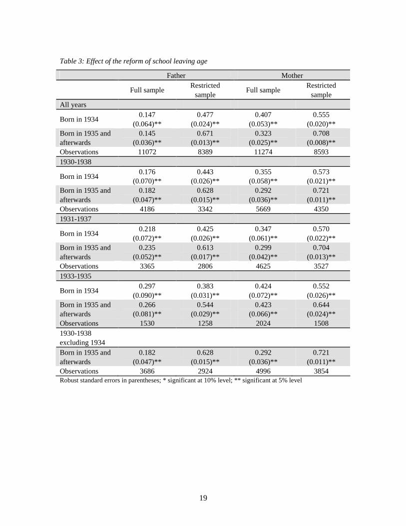
We estimate the effect of the reform on the age at which fathers and mothers leave
school. We capture the effect of the reform by a dummy for whether the individual was 14 on the
year the reform was implemented and on the subsequent years it was in place. Since the reform
might not fully affect the 1934 cohort like the later birth cohorts, we look at the effect of being
born in 1934 and of being born in 1935 and afterwards. Additionally, for comparison purposes,
we re-estimate the same model excluding those born in 1934. We perform the regressions for
different birth year intervals and we also compare the effect on the entire education distribution
(full sample) and only those finishing at ages 14 and 15 (restricted sample). The results are
reported in Table 3 and show that the education reform had a higher impact on the restricted
sample of lower educated individuals. For the restricted sample both the coefficients are higher
and the standard errors are lower. For the full sample, the reform in 1947 increased the mother’s
education by 0.407 years. The increase for the lower educated (restricted) was 0.555 years. For
males this difference was even bigger (the coefficient increased from 0.147 to 0.477). This indeed
confirms that the reform mainly affected the educational choices of those individuals at the lower
end of the educational distribution. Furthermore, there seems to be some sensitivity of the
reform’s impact to the sample of birth cohorts chosen. When looking at all education ages, it
appears that the reform had a slightly larger effect for those born in 1934. The reverse is true for
the sample of people leaving at ages 14 and 15: those born in 1935 and afterwards experienced a
greater increase in education than those born in 1934. In addition, the effect of the reform slightly
decreases as birth cohorts closer in time are taken into account.

7
4 Estimation methods
The schooling reform provides a natural experiment that can be used to identify the causal impact
of parental schooling on a number of different outcome measures. Since close to the reform
individuals are expected to be similar except for exposure to the reform, we can use regression-
discontinuity techniques. The design is fuzzy as the school leaving age does not deterministically
depend on exposure to the reform (e.g. Hahn, Todd and Van der Klaauw, 2001). Obviously prior
to the reform some individuals left school at age 15 or later, but also after the reform still some
individuals left school at age 14. Since exposure to the reform depends on the year of birth, the
regression-discontinuity design suggests that we should compare individuals born close to 1934,
which was the first birth cohort affected by the reform. In the fuzzy regression-discontinuity
design parental education is instrumented by whether or not they were exposed to the reform. Our
empirical model is summarized by the following three equations:
εββββββββ ++++++++= mfmf AARPSEEH 76543210 (1)
E Y S P R Af f f= + + + + + +δ δ δ δ δ δ γ0 1 2 3 4 5 (2)
E Y S P R Am m m= + + + + + +δ δ δ δ δ δ υ0 1 2 3 4 5 (3)
H represents child health, E is the age at which the father and mother finished school, S is the sex
of the child, P is parity in 1958, R includes dummy variables for the region of residence, A
includes the age of the father and the mother in 1958, and Y is a dummy for whether the
individual was affected by the reform. The superscript f indicates that the variable relates to the
father, while the superscript m relates to the mother.
An important reason for including parity of the child and parental age is to reduce
potential biases that might arise because the sample consists of families having a child born in
1958. It cannot be ruled out that the schooling reform affects fertility decisions such as the timing
of childbearing and/or the number of children. We have checked the effect of the reform on parity
in 1958 and on total fertility as observed in the 1974 survey and we did not find a significant
effect of the reform in these regressions. Nevertheless, it is possible that the reform affects the
decision to have any children at all or to delay childbearing. Furthermore, parents affected by the
reform were born in later years than parents not affected by the reform. This implies that the
parents affected by the reform were younger in 1958 when the child was born. We expect that
controlling for parity and parental age reduces potential biases, but we cannot rule out that some

8
biases remain. It has to be noted that the same criticism applies to the study by McCrary and
Royer (2006) who condition on mothers having their first child before age 23.
This model will estimate the causal effects of parental education on a range of child
health variables: the child’s birth weight, whether the child had an illness at birth, the number of
chronic conditions in later childhood, height-for-age-z-scores and Body Mass Index. The results
of these analyses will be discussed in Subsection 5.1.
As mentioned earlier, the impact of parental education may act on child health through
various channels. Firstly, it may be that higher educated parents have more knowledge about
prenatal care and care-taking of children and therefore for example they smoke less during
pregnancy or more often breastfeed their child. Secondly, it is possible that increased education
may have a direct impact on parents’ health and that better parental health is transmitted across
generations. Thirdly, health benefits might come from increased earnings or changed labor supply
choices (particularly for women). We will also examine whether there is a causal effect of
education on parental outcome variables such as: maternal smoking, whether the child was
breastfed, an indicator of a chronic condition for the father or mother, father’s Body Mass Index,
or mother’s Body Mass Index, the work status of the mother and whether the family experienced
financial difficulties. The results of these analyses will be discussed in Subsection 5.2.
Identification from the regression-discontinuity design assumes that the population
affected by the reform and the population not affected by the reform differ only in exposure to the
reform. In practice, this assumption is justified only if the sample consists of birth cohorts
sufficiently close to 1934 in order to avoid other cohort and trend effects. Indeed, children born to
older parents might face a different socioeconomic environment than those born to younger
parents, which might affect the outcomes of interest. We estimate our model for different
subsamples of birth cohorts. It is obvious that if we restrict the subsample to only a few birth
cohorts, we have a relatively small sample size. On the other hand if we take a subsample with
many birth cohorts, other cohort and trend effects might bias the estimated effects. When
restricting to a subsample of particular birth cohorts, we include only families with both parents
born in the included birth years. As mentioned in the previous subsection, in 1934 there might
have been only partial compliance to the reform. Therefore, as instrumental variables in equations
(2) and (3), we include separate dummy variables for being born in 1934 and for being born in
1935 or later. Furthermore, we construct subsamples from which we exclude families with
parents born in 1934. As mentioned in the previous section, the reform only affected the behavior
of those individuals for which the reform was binding. The fraction of individuals leaving school
at age 16 or later did not change due to the reform. We estimate our model both for the full

9
sample containing individuals with all levels of education and a restricted sample containing only
individuals who left school at age 14 or 15. The interpretation of the coefficients 1β and 2β
differs between both sample choices. In case we use the full sample, the coefficients describe
homogenous effects of education. We have shown that the reform affected only individuals in the
lower part of the educational distribution. This implies that if we use the full sample, the linear
first stage regressions (2) and (3) are wrongly specified. If we use the restricted sample, the
coefficients 1β and 2β should be interpreted as local effect of schooling, since these coefficient
only measure educational effects for those parents persuaded to obtain one additional year of
education due to the reform. Under the assumption that no individual will lower his/her level of
education due to the reform (monotonicity assumption), our estimated effects should be
interpreted within the local average treatment effect framework (Imbens and Angrist, 1994). In
particular, this implies that our estimated effects are the educational effects for those individuals
who due to the reform increased their school leaving age from 14 to 15. From the previous
section we have seen that this is about 50% of a birth cohort. The results are nevertheless
interesting from a policy point of view because they focus on those at the bottom of the education
distribution, the same group that is often aimed at in public programs.
5 Results
5.1 Child health
The OLS estimation results for equation (1) are presented in Table 4. The table includes the effect
of parental education on infant health at the time of birth (measured by birth weight and whether
or not the child has an illness at birth) and at later ages in childhood (the number of conditions
and height-for-age-z-scores and Body Mass Index at ages 7, 11 and 16). We present the results
for different samples of birth cohorts and education groups. The OLS estimates show some
significant associations between parental education and indicators for their offspring’s health at
birth. Higher birth weight is related to more parental education (either father or mother depending
on the sample). The coefficient is also higher when focusing on the restricted sample with less
educated parents. There is, on the other hand no effect of parental education on the probability of
an illness at birth (the sample of less educated parents born in 1933-1935 being the exception).
For later childhood health, the full sample shows that there exists a positive association
between parental schooling and child health when looking at anthropometric measures. Both
maternal and paternal education levels are associated with higher height-for-age-z-scores for

10
children. When we focus on fewer birth years around the year of the reform, we find only
maternal education to be significantly associated with higher height-for-age-z-scores. Father’s
education is correlated with Body Mass Index; more years of schooling for the father are
associated with lower Body Mass Index. For the full sample, we never find a significant
association between either father’s or mother’s education and the number of conditions during
later childhood. We find no significant association between parental education and the child’s
health measures between ages 7 to 16 for the sample of lower educated parents.
Table 5 presents the instrumental variables (IV) results. We instrument the age at which
the parents left school by whether they were affected by the reform. Almost all results are
statistically insignificant, suggesting that there is no causal effect of increased parental education.
Compared to the OLS results, the lack of significance is not always caused by reduced parameter
estimates. For example, for the number of conditions and for height-for age-z-scores, we quite
often see that both the estimated coefficients and the standard error increases. For the sample of
parents leaving school at age 14-15 we find only that father’s education has a marginally
significant effect on the probability of having an illness at birth. But this effect is only present in
the subsample of the birth cohorts 1931-1937 and disappears in the other subsamples of birth
cohorts.
Epidemiological and economic studies on the long run effects of poor infant health often
find different results for boys and girls. For instance, Leon et al. (1998) find that the relationship
between birth weight and death from ischaemic heart disease is significant for men and not for
women. Similarly, Van den Berg. Lindeboom and Portrait (2006) find that being born in a
recession increases mortality risk at later ages and that this effect is only significant for men. We
therefore also performed separate IV analyses for boys and girls. This did not alter the results. In
none of the analyses we found any significant effect of parental education on the infant’s health.
In the economic literature intergenerational effects are most often estimated separately
for fathers and mothers (Black, Devereux and Salvanes, 2005; Holmlund, Lindahl and Plug,
2006). The interpretation of the coefficients of education in separate regressions differs from
those in our model where both father’s and mother’s education are included. In particular, when
separate regressions are done for the father and mother, the estimated effects also include the
effects of whom he/she marries (Behrman and Rosenzweig, 2002). Effects of assortative mating
on education are thus included in the parameter estimate of the education coefficient when one
performs separate regressions for both parents. In a model where the education of both parents is
included one can interpret the results as the direct effects of each parents’ education. However,
more importantly, performing separate analyses for fathers and mothers can lead to inconsistent

11
estimates in the case of assortative mating, even if one performs IV analyses. The main reasoning
behind this is that if the father and mother are close in age, the reform is not a valid instrumental
variable anymore. If one parent is affected by the reform, this increases the probability that also
the partner is also affected by the reform. Therefore, the increased education of the partner does
not only run via the educational level of the parent, but also via the reform. Since the educational
level of the partner is not included as regressor, it is absorbed in the error term of the second
stage. Assortative matching on age thus causes that the variables describing the reform are
correlated with the second-stage error terms, which violates the validity condition for
instrumental variables. Our data shows that the correlation between year of birth of the father and
mother is 0.79. The correlation for exposure to the reform is 0.53, while the correlation in years
of education is 0.57.
It is, however, interesting to see how the effects of education change if we do
separate analyses for fathers and mothers. The results from IV estimation for mothers and
fathers are presented in Table 6 and 7 respectively. Most effects for parental education
are very small and not significant. For mothers, we only find in the 1933-1935 sample
that more education reduces the height-for-age-z-score. For fathers we find similarly in
the 1933-1935 sample a significant negative effect of education on the height-for-age-z-
score.
5.2 Parental outcomes
We found little evidence for a causal impact of parental education on child heath. In the
introduction we have specified a number of channels through which parental education could
affect child health. In particular, we mentioned that parental education may affect child health
indirectly via parental behavior, parental health and parental financial resources. By investigating
the causal impact of education on these parental outcomes measures, we might be able to rule out
whether these parental outcomes might affect child health. The underlying idea is that when
parental education for example significantly increases parental financial resources, it is very
unlikely that parental financial resources have a substantial impact on child health, given that we
do not find any effect of parental education on child health. In Table 8 we show results from OLS
estimation for the effect of parental education on parental outcomes. Table 9 presents the IV
results.
12
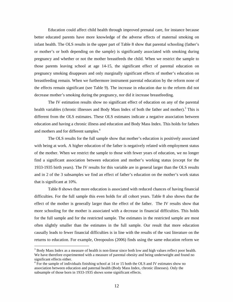
Education could affect child health through improved prenatal care, for instance because
better educated parents have more knowledge of the adverse effects of maternal smoking on
infant health. The OLS results in the upper part of Table 8 show that parental schooling (father’s
or mother’s or both depending on the sample) is significantly associated with smoking during
pregnancy and whether or not the mother breastfeeds the child. When we restrict the sample to
those parents leaving school at age 14-15, the significant effect of parental education on
pregnancy smoking disappears and only marginally significant effects of mother’s education on
breastfeeding remain. When we furthermore instrument parental education by the reform none of
the effects remain significant (see Table 9). The increase in education due to the reform did not
decrease mother’s smoking during the pregnancy, nor did it increase breastfeeding.
The IV estimation results show no significant effect of education on any of the parental
health variables (chronic illnesses and Body Mass Index of both the father and mother).3 This is
different from the OLS estimates. These OLS estimates indicate a negative association between
education and having a chronic illness and education and Body Mass Index. This holds for fathers
and mothers and for different samples.4
The OLS results for the full sample show that mother’s education is positively associated
with being at work. A higher education of the father is negatively related with employment status
of the mother. When we restrict the sample to those with fewer years of education, we no longer
find a significant association between education and mother’s working status (except for the
1933-1935 birth years). The IV results for this variable are in general larger than the OLS results
and in 2 of the 3 subsamples we find an effect of father’s education on the mother’s work status
that is significant at 10%.
Table 8 shows that more education is associated with reduced chances of having financial
difficulties. For the full sample this even holds for all cohort years. Table 8 also shows that the
effect of the mother is generally larger than the effect of the father. The IV results show that
more schooling for the mother is associated with a decrease in financial difficulties. This holds
for the full sample and for the restricted sample. The estimates in the restricted sample are most
often slightly smaller than the estimates in the full sample. Our result that more education
causally leads to fewer financial difficulties is in line with the results of the vast literature on the
returns to education. For example, Oreopoulos (2006) finds using the same education reform we
3 Body Mass Index as a measure of health is non-linear since both low and high values reflect poor health. We have therefore experimented with a measure of parental obesity and being underweight and found no significant effects either. 4 For the sample of individuals finishing school at 14 or 15 both the OLS and IV estimates show no association between education and paternal health (Body Mass Index, chronic illnesses). Only the subsample of those born in 1933-1935 shows some significant effects.

13
use large and significant earnings returns to education. It is generally found that more education
leads to higher earnings and that the IV results are generally larger than the OLS results (see for
instance the survey of Card, 1999).
The significant causal effect of education on parental income sheds some more light on
the potential effect of income in determining child health. Given that parental education has a
causal effect on financial resources but no direct effect on the child health, we can conclude that
parental income can at most have a very modest effect on child health. For the population of
parents affected by the reform we do not find any effect of education on own health or on
parental care. Therefore, our results do not rule out that parental health and/or parental
care are important for child health.
6 Discussion and Conclusion
We examined the intergenerational effects of education on child health. As in most of the
empirical literature, our data shows a strong positive association between parental socioeconomic
status and child health. To investigate the causality of the relationship, we have exploited
exogenous variation in parental educational due to a schooling reform on the minimum school
leaving age. We have shown that the schooling reform only affected the educational decisions of
individuals at the lower end of the educational distribution. In particular, about 50% of all
individuals in a birth cohort were affected. The education reform appears to have had a
substantial positive effect on time in schooling. For males additional schooling can be as high as
0.6 years, for females this is 0.7 years. Our results provide little evidence of a direct causal effect
of parental education on child health. There is however more robust evidence of the positive
effect of increasing education on living standards since an extra year of schooling decreases the
household’s financial difficulties. Given the fact that education has a causal impact on financial
resources but little impact on child health, this raises the question as to what extent parental
income does influence offspring health outcomes. For the population that is affected by the
reform we do not find any effect of education on parental health or on parental care. Therefore
our results do not rule out that parental health and/or parental care are important for child health.
Our findings are line with finding from the literature on the intergenerational
transmission of education. Black, Devereux and Salvanes (2003) use a change in the educational
system in Norway to assess the causal effect of parental education on the child’s education. They
also do not find a causal effect from parental education. They conclude from their findings that

14
the intergenerational correlation in education is due to family circumstances and/or inherited
ability. This may also be the case for child health.
It is interesting to compare our findings to two studies on the intergenerational effects of
education on child health. Currie and Moretti (2003) find significant improvement of infant health
for women attending College. This seems to contrast our findings. However, they argue that the
improvements in child health come from increases in prenatal care and reduced smoking due to
the higher education of the mother. We did not find any changes in prenatal behavior or child care
due to the increased schooling. Our results are completely in line with McCrary and Royer
(2006). They exploit discontinuities in school entry policies. In their set up the discontinuities can
lead to 0.14 to 0.25 fewer years of education for those born beyond the school entry date. This
change is substantially smaller than the changes in our sample induced by the reform. They
examine the effect of education for those mothers giving birth before the age of 23 and find
limited returns to education. They argue that this is because they focus on a sample of low
educated women at risk of dropping out of school (like in our sample). Alternatively, the
differences in results between Currie and Moretti (1999) on the one hand and our study and
McCrary and Royer (2006) on the other hand can be explained by the fact that the type of policy
is different: our study focuses on a policy manipulating time of exit while Currie and Moretti
(2003) look at a policy promoting College entrance.5 The policies thus interfere at different
margins of the parental educational distribution. One might take from combining the studies that
positive intergenerational effects on child health appear when the parents reach a sufficiently high
educational level. Besides most of those affected by the 1947 reform went into general secondary
education and one could argue that because of this the value added of the additional year of
schooling was very small. So, the quality of education rather than the quantity of education is
important.
5 McCrary and Royer (2006) is more similar to our study as they also consider low educated mothers and they focus on the time in school of these women.

15
References Arendt, J.N. (2005), Does Education Cause Better Health? A Panel Data Analysis Using School Reforms for Identification, Economics of Education Review 24, 149-160. Behrman, J.R. and M.R. Rosenzweig (2002), Does Increasing women’s Schooling Raise the Schooling of the Next Generation?, American Economic Review 92, 323-334. Black, S., P. Devereux and K. Salvanes (2005), Why the Apple Doesn’t Fall Far: Understanding the Intergenerational Transmission of Education, American Economic Review 95, 437-449. Card, D. (1999), The Causal Effect of Education on Earnings, in O.C. Ashenfelter and D. Card (eds.), Handbook of Labor Economics, Volume 3A, North-Holland. Case, A., A. Fertig and C. Paxson (2005), The Lasting Impact on Childhood Health and Circumstance, Journal of Health Economics 24, 365-389. Case, A., M. Lubotsky and C. Paxson (2002), Economic Status and Health in Childhood: The Origins of the Gradient, American Economic Review 92, 1308-1334. Chevalier, A., C. Harmon, V. O’Sullivan and I. Walker (2005), The Impact of Parental Income and Education on the Schooling of their Children. IZA Discussion Papers Series, Discussion Paper 1496. Currie, J. and E. Moretti (2003), Mother’s Education and the Intergenerational Transmission of Human Capital: Evidence from College Openings, Quarterly Journal of Economics 118, 1495-1532. Currie, A., M.A. Shields and S. Wheatley-Price (2006), Is the Child Health / Family Income Gradient Universal?, Journal of Health Economics, forthcoming. Currie, J. and M. Stabile (2003), Socioeconomic Status and Child Health: Why Is the Relationship Stronger for Older Children?, American Economic Review 93, 1813-1823. Cutler, D.M. and A. Lleras-Muney (2006), Education and Health: Evaluating Theories and Evidence. National Bureau Economic Research Working Paper Series, Working Paper 12352. Doyle, O., C. Harmon, I. Walker (2005), The Impact of Parental Income and Education on the Health of their Children, IZA Discussion Paper Series, Discussion Paper 1832. Galindo-Rueda, F. (2003), The Intergenerational Effect of Parental Schooling: Evidence from the British 1947 School Leaving Reform, Centre for Economic Performance, mimeo. Hahn, J., P. Todd and W. van der Klaauw (2001), Identification and Estimation of Treatment Effects with a Regression-Discontinuity Design, Econometrica 69, 201-209. Harmon, C. and I. Walker (1995), Estimates of the Economic Return to Schooling for the United Kingdom, American Economic Review 85, 1278-1296.

16
Holmlund, H., M. Lindahl and E. Plug (2006), Estimating Intergenerational Schooling Effects: A Comparison of Methods, Mimeo. Imbens, G.W. and J.D. Angrist (1994), Identification and Estimation of Local Average Treatment Effects, Econometrica 62, 467-475. Leon, D.A., H.O. Lithell, D. Vågerö, I. Koupilová, R. Mohsen, L. Berglund, U-B. Lithell and P.M. McKeigne (1998), Reduced Fetal Growth Rate and Increased Risk of Death from Ischaemic Heart Disease: Cohort Study of 15 000 Swedish Men and Women Born 1915-29. British Medical Journal 317, 241-245. Lleras-Muney, A. (2005), The Relationship Between Education and Adult Mortality in the United States, Review of Economic Studies 72, 189-221. McCrary, J. and H. Royer (2006), The Effect of Female Education on Fertility and Infant Health: Evidence from School Entry Policies Using Exact Date of Birth, University of Michigan, Working Paper. Meghir, C. and M. Palme (2005), Educational Reform, Ability and Parental Background, American Economic Review 95, 414-424. Oreopoulos, P. (2006), Estimating Average and Local Average Treatment Effects of Education When Compulsory Schooling Laws Really Matter, American Economic Review 96, 152-175. Oreopoulos, P., M.E. Page and A.H. Stevens (2006), The Intergenerational Effects of Compulsory Schooling, Journal of Labor Economics 24, 729-760. Pischke, J.-S. and T. von Wachter (2005) Zero Returns to Compulsory Schooling in Germany: Evidence and Interpretation, National Bureau Economic Research Working Paper Series, Working Paper 11414. Power, C. and C. Peckham (1987), Childhood Morbidity and Adult Ill-Health, National child Development Study User Support Group, Working Paper No. 37. Van den Berg, G.J., M. Lindeboom and F. Portrait (2006), Economic Conditions Early In Life and Individual Mortality, American Economic Review 96, 290-302.

17
Table 1: Parental and child variables by level of parental schooling
Fathers Mothers
14 15 16+ 14 15 16+
Financial difficulties in the
family
(Avg over 1965, 1969, 1974)
9.56% 9.75% 3.09% 10.57% 9.79% 3.86%
Mother works
(Avg over 1965, 1969, 1974) 53.23% 59.52% 48.96% 57.85% 59.39% 53.53%
Father chronic conditions
(Avg over 1969, 1974) 8.26% 4.78% 4.03% 8.62% 5.63% 4.52%
Mother chronic conditions
(Avg over 1969, 1974) 6.19% 5.64% 4.24% 6.68% 5.41% 4.26%
Father obese in 1974 5.01% 3.41% 3.49% 5.05% 3.69% 3.86%
Mother obese in 1974 8.08% 5.67% 2.68% 7.87% 6.54% 3.24%
Maternal smoking during
pregnancy 36.20% 31.63% 24.57% 37.71% 33.42% 21.81%
Breastfeeding 64.98% 71.36% 76.47% 63.19% 72.36% 75.54%
Child birth weight in kg 3.34 3.31 3.39 3.35 3.30 3.39
Child illness at birth 3.03% 2.23% 2.41% 3.19% 2.63% 2.13%
Child number of conditions
(Avg over 1965, 1969, 1974) 2.17 2.16 2.07 2.15 2.22 2.10
Child stunt
(Avg over 1965, 1969, 1974) 2.68% 2.69% 1.03% 2.58% 2.85% 1.12%
Child obese
(Avg over 1965, 1969, 1974) 4.42% 3.28% 3.09% 4.67% 3.27% 3.10%

18
Table 2: Distribution of parents schooling by year of birth
Fathers Mothers Mean SD Freq. Mean SD Freq.
1927 14,96 2,11 1644 14,81 1,74 1254 1928 14,94 1,93 1947 14,83 1,64 1557 1929 14,94 2,00 2019 14,84 1,67 1905 1930 15,03 2,03 2133 14,86 1,62 1857 1931 14,99 1,92 1989 14,92 1,71 2316 1932 14,86 1,62 1977 14,96 1,71 2040 1933 14,79 1,65 1785 14,82 1,39 2055 1934 15,09 1,35 1500 15,24 1,29 2019 1935 15,06 0,94 1305 15,25 1,04 1986 1936 15,14 1,14 966 15,17 0,98 1860 1937 15,15 1,08 588 15,19 0,87 1608 1938 15,01 0,73 330 15,12 0,68 1245 1939 15,03 0,74 174 15,09 0,65 744
19
Table 3: Effect of the reform of school leaving age
Father Mother
Full sample Restricted
sample Full sample
Restricted sample
All years
Born in 1934 0.147
(0.064)** 0.477
(0.024)** 0.407
(0.053)** 0.555
(0.020)** Born in 1935 and afterwards
0.145 (0.036)**
0.671 (0.013)**
0.323 (0.025)**
0.708 (0.008)**
Observations 11072 8389 11274 8593 1930-1938
Born in 1934 0.176
(0.070)** 0.443
(0.026)** 0.355
(0.058)** 0.573
(0.021)** Born in 1935 and afterwards
0.182 (0.047)**
0.628 (0.015)**
0.292 (0.036)**
0.721 (0.011)**
Observations 4186 3342 5669 4350 1931-1937
Born in 1934 0.218
(0.072)** 0.425
(0.026)** 0.347
(0.061)** 0.570
(0.022)** Born in 1935 and afterwards
0.235 (0.052)**
0.613 (0.017)**
0.299 (0.042)**
0.704 (0.013)**
Observations 3365 2806 4625 3527 1933-1935
Born in 1934 0.297
(0.090)** 0.383
(0.031)** 0.424
(0.072)** 0.552
(0.026)** Born in 1935 and afterwards
0.266 (0.081)**
0.544 (0.029)**
0.423 (0.066)**
0.644 (0.024)**
Observations 1530 1258 2024 1508 1930-1938 excluding 1934
Born in 1935 and afterwards
0.182 (0.047)**
0.628 (0.015)**
0.292 (0.036)**
0.721 (0.011)**
Observations 3686 2924 4996 3854 Robust standard errors in parentheses; * significant at 10% level; ** significant at 5% level

20
Table 4: Parents education and child’s health- OLS
Full sample Parents finishing at age 14-15
Birth w
eight
Illness at birth
Num
ber of conditions
Height-for
age-Z scores
Body M
ass Index
Birth w
eight
Illness at birth
Num
ber of conditions
Height-for
age-Z scores
Body M
ass Index
1930-1938
Father 0.007
(0.006)
0.000
(0.002)
0.000
(0.015)
0.028
(0.013)**
-0.040
(0.026)
0.084
(0.026)**
0.008
(0.008)
-0.110
(0.069)
0.073
(0.054)
0.049
(0.109)
Mother 0.020
(0.008)**
-0.001
(0.003)
-0.014
(0.021)
0.039
(0.016)**
-0.002
(0.034)
-0.035
(0.029)
-0.008
(0.009)
-0.011
(0.075)
-0.062
(0.057)
-0.085
(0.119)
P-value joint 0.000 0.951 0.725 0.000 0.150 0.006 0.515 0.238 0.314 0.752
Observations 3331 3459 8186 7921 7921 2287 2381 5609 5415 5415
1931-1937
Father 0.005
(0.007)
-0.003
(0.002)
-0.009
(0.018)
0.026
(0.015)*
-0.085
(0.029)**
0.080
(0.030)**
0.005
(0.010)
-0.116
(0.085)
0.046
(0.062)
-0.035
(0.131)
Mother 0.018
(0.010)*
0.001
(0.003)
-0.021
(0.025)
0.041
(0.019)**
0.029
(0.041)
-0.015
(0.033)
-0.001
(0.010)
-0.021
(0.091)
-0.037
(0.066)
-0.117
(0.144)
P-value joint 0.023 0.496 0.367 0.000 0.008 0.028 0.834 0.304 0.726 0.625
Observations 2345 2434 5740 5543 5543 1606 1669 3928 3786 3786
1933-1935
Father 0.014
(0.017)
0.009
(0.006)
-0.057
(0.043)
0.018
(0.027)
-0.171
(0.058)**
0.088
(0.055)
-0.200
(0.100)*
-0.231
(0.142)
-0.029
(0.105)
-0.357
(0.243)
Mother 0.013
(0.019)
-0.008
(0.007)
0.001
(0.054)
0.080
(0.034)**
0.165
(0.080)**
-0.109
(0.058)*
-0.021
(0.119)
-0.077
(0.154)
-0.048
(0.112)
-0.355
(0.276)
P-value joint 0.396 0.311 0.344 0.008 0.011 0.109 0.099 0.133 0.812 0.027
Observations 543 561 1321 1288 1288 372 2365 900 868 868
1930-1938, excluding 1934
Father -0.000
(0.007)
0.000
(0.002)
0.017
(0.017)
0.023
(0.015)
-0.058
(0.028)**
0.099
(0.032)**
0.010
(0.010)
-0.023
(0.084)
0.047
(0.066)
0.082
(0.128)
Mother 0.028
(0.009)
-0.002
(0.003)
-0.024
(0.022)
0.047
(0.018)**
0.006
(0.039)
-0.002
(0.004)
-0.011
(0.011)
-0.063
(0.091)
-0.062
(0.068)
-0.092
(0.141)
P-value joint 0.002 0.785 0.487 0.000 0.042 0.006 0.483 0.697 0.599 0.719
Observations 2532 2612 6221 6032 6032 1746 1816 4282 4151 4151
Robust standard errors in parentheses; * significant at 10% level; ** significant at 5% level. For each interval, both the mother and the father are born within those years. Regressions are performed for children living with their natural parents and include sex of child, parity, regional dummies, and parental age. The results for the number of conditions, height-for age-Z scores and Body Mass Index are based on observations when the child was 7, 11 and 16 years old. We control for the age of the child and the estimation includes clustered standard errors. Disaggregated analyses are available upon request.

21
Table 5: Parents education and child’s health – IV
full sample Parents finishing at age 14-15 B
irth weight
Illness at birth
Num
ber of conditions
Height-for ag
e-Z
-scores
Body M
ass Index
Birth w
eight
Illness at birth
Num
ber of conditions
Height-for ag
e-Z
-scores
Body M
ass Index
1930-1938
Father 0.094
(0.091)
0.002
(0.027)
0.134
(0.209)
0.091
(0.151)
-0.301
(0.327)
0.049
(0.099)
-0.018
(0.031)
-0.066
(0.241)
-0.058
(0.190)
-0.458
(0.391)
Mother -0.121
(0.078)
0.000
(0.023)
0.116
(0.195)
-0.059
(0.142)
-0.175
(0.313)
-0.145
(0.075)*
-0.005
(0.023)
0.058
(0.184)
-0.145
(0.139)
-0.382
(0.296)
P-value joint 0.253 0.997 0.556 0.810 0.460 0.152 0.810 0.929 0.519 0.165
Observations 3331 3459 8186 7921 7921 2287 2381 5609 5415 5415
1931-1937
Father 0.087
(0.137)
-0.017
(0.040)
0.183
(0.353)
0.024
(0.257)
-0.285
(0.580)
0.172
(0.138)
-0.073
(0.043)*
-0.036
(0.349)
-0.018
(0.272)
-0.070
(0.572)
Mother -0.105
(0.127)
0.006
(0.036)
0.241
(0.320)
-0.231
(0.234)
-0.418
(0.483)
-0.045
(0.097)
0.009
(0.030)
0.128
(0.245)
-0.214
(0.186)
-0.482
(0.388)
P-value joint 0.533 0.885 0.655 0.609 0.625 0.459 0.241 0.870 0.471 0.411
Observations 2345 2434 5740 5543 5543 1606 1669 3928 3786 3786
1933-1935
Father -0.025
(0.105)
-0.012
(0.035)
0.055
(0.278)
-0.056
(0.162)
-0.301
(0.454)
0.024
(0.121)
-0.011
(0.039)
0.102
(0.305)
-0.388
(0.243)
-0.832
(0.574)
Mother -0.240
(0.187)
-0.054
(0.060)
-0.525
(0.568)
0.105
(0.381)
-0.095
(0.822)
-0.098
(0.109)
-0.030
(0.035)
-0.363
(0.294)
-0.062
(0.216)
1.380
(1.121)
P-value joint 0.437 0.652 0.564 0.872 0.791 0.656 0.554 0.457 0.107 0.284
Observations 543 561 1321 1288 1288 372 386 900 868 868
1930-1938, excluding 1934
Father 0.183
(0.178)
-0.006
(0.046)
0.161
(0.330)
-0.037
(0.258)
-0.011
(0.525)
0.094
(0.120)
-0.013
(0.038)
-0.049
(0.286)
-0.125
(0.234)
-0.014
(0.455)
Mother -0.201
(0.142)
0.035
(0.037)
0.059
(0.305)
-0.132
(0.226)
-0.497
(0.467)
-0.153
(0.097)
0.031
(0.030)
0.026
(0.230)
-0.316
(0.174)
-0.567
(0.360)
P-value joint 0.362 0.544 0.688 0.668 0.396 0.262 0.595 0.982 0.132 0.277
Observations 2532 2629 6221 6032 6032 1746 1816 4282 4151 4151
Robust standard errors in parentheses; * significant at 10% level; ** Significant at 5% level. For each interval, both the mother and the father are born within those years. The regressions are performed for those children with their natural parents. Extra controls as in Table 4.

22
Table 6:Separate analyses: Mother’s education and child’s health IV
full sample finishing at age 14-15 B
irth weight
Illness at birth
Num
ber of conditions
Height-for ag
e-Z
-scores
Body M
ass Index
Birth w
eight
Illness at birth
Num
ber of conditions
Height-for ag
e-Z
-scores
Body M
ass Index
1930-1938
Mother -0.063
(0.071)
-0.009
(0.022)
0.041
(0.162)
0.063
(0.127)
-0.201
(0.278)
-0.094
(0.057)
-0.005
(0.019)
-0.007
(0.143)
-0.061
(0.107)
-0.395
(0.231)
Observations 5337 5515 13043 12618 12618 4094 4229 9952 9601 9601
1931-1937
Mother -0.029
(0.073)
-0.009
(0.023)
0.010
(0.164)
0.096
(0.130)
-0.125
(0.281)
-0.057
(0.067)
-0.008
(0.022)
-0.005
(0.167)
-0.004
(0.126)
-0.374
(0.269)
Observations 4342 4496 10625 10277 10277 3313 3426 8054 7761 7761
1933-1935
Mother -0.107
(0.067)
-0.020
(0.020)
0.083
(0.150)
-0.093
(0.120)
-0.206
(0.260)
-0.109
(0.047)**
-0.015
(0.016)
0.053
(0.118)
-0.161
(0.088)*
-0.266
(0.188)
Observations 1908 1971 4678 4531 4531 1426 1466 3469 3335 3335
1930-1938, excluding 1934
Mother -0.073
(0.103)
0.011
(0.031)
-0.022
(0.225)
0.059
(0.175)
-0.329
(0.392)
-0.101
(0.065)
0.006
(0.022)
-0.010
(0.164)
-0.060
(0.121)
-0.423
(0.262)
Observations 4707 4861 11460 11075 11075 3627 3747 8795 8480 8480
Robust standard errors in parentheses; * significant at 10% level; ** significant at 5% level. The regressions are performed for those children with their natural parents. Extra controls as in Table 4.

23
Table 7: Separate analyses: Father’s education and child’s health IV
full sample finishing at age 14-15 B
irth weight
Illness at birth
Num
ber of conditions
Height-for ag
e-Z
-scores
Body M
ass Index
Birth w
eight
Illness at birth
Num
ber of conditions
Height-for ag
e-Z
-scores
Body M
ass Index
1930-1938
Father 0.034
(0.090)
-0.011
(0.028)
0.108
(0.224)
-0.043
(0.177)
-0.393
(0.376)
-0.003
(0.084)
-0.010
(0.027)
0.053
(0.216)
-0.135
(0.175)
-0.424
(0.356)
Observations 3944 4093 9614 9291 9291 3141 3266 7650 7392 7392
1931-1937
Father 0.016
(0.112)
-0.035
(0.036)
0.219
(0.319)
0.011
(0.239)
-0.321
(0.514)
-0.026
(0.105)
-0.029
(0.033)
0.077
(0.279)
-0.247
(0.230)
-0.505
(0.464)
Observations 3167 3286 7692 7423 7423 2543 2645 6193 5973 5973
1933-1935
Father -0.019
(0.104)
-0.010
(0.033)
0.422
(0.355)
-0.181
(0.236)
-0.445
(0.494)
-0.009
(0.063)
-0.017
(0.019)
0.150
(0.165)
-0.237
(0.130)*
-0.286
(0.256)
Observations 1444 1496 3475 3362 3362 1182 1227 2837 2735 2735
1930-1938, excluding 1934
Father 0.056
(0.101)
-0.015
(0.031)
-0.057
(0.243)
-0.118
(0.209)
-0.308
(0.421)
0.034
(0.091)
-0.011
(0.029)
-0.089
(0.229)
-0.161
(0.186)
-0.239
(0.375)
Observations 3468 3601 8479 8219 8219 2764 2874 6751 6553 6553
Robust standard errors in parentheses; * significant at 10% level; ** significant at 5% level. The regressions are performed for those children with their natural parents. Extra controls as in Table 4.

24
Table .8: Parental education on parental variables –OLS results
Maternal smoking during pregnancy
Breastfeeding Father Illness
Mother Illness
Body Mass Index Father
Body Mass Index Mother
Mother work
Financial difficulties
All education years 1930-1938
Father -0.012
(0.006)**
0.022
(0.006)**
-0.008
(0.002)**
-0.004
(0.002)*
-0.104
(0.043)**
-0.179
(0.054)**
-0.018
(0.005)**
-0.009
(0.002)**
Mother -0.025
(0.008)**
0.018
(0.008)**
0.000
(0.003)
-0.001
(0.003)
-0.077
(0.054)
-0.105
(0.067)
0.013
(0.006)**
-0.008
(0.002)**
P-value 0.000 0.000 0.000 0.018 0.000 0.000 0.003 0.000
Observations 3459 3121 5966 5966 2849 2849 8947 8906
1933-1935
Father -0.027
(0.016)*
0.029
(0.016)*
-0.018
(0.006)**
-0.006
(0.007)
-0.115
(0.114)
-0.188
(0.134)
-0.007
(0.015)
-0.008
(0.004)*
Mother -0.001
(0.019)
0.012
(0.018)
0.002
(0.007)
-0.001
(0.008)
-0.156
(0.132)
-0.084
(0.159)
0.025
(0.014)*
-0.014
(0.005)**
P-value 0.184 0.053 0.002 0.484 0.113 0.175 0.181 0.000
Observations 561 495 970 970 463 463 1449 1446
1930-1938 except 1934
Father -0.008
(0.007)
0.020
(0.007)**
-0.008
(0.002)**
-0.003
(0.002)
-0.116
(0.049)**
-0.222
(0.061)**
-0.019
(0.006)**
-0.008
(0.002)**
Mother -0.031
(0.009)**
0.023
(0.008)**
0.001
(0.003)
0.000
(0.003)
-0.040
(0.061)
-0.075
(0.076)
0.016
(0.007)**
-0.009
(0.002)**
P-value 0.000 0.000 0.000 0.164 0.002 0.000 0.006 0.000
Observations 2629 2373 4529 4529 2159 2159 6794 6761
Left school at 14-15 1930-1938
Father -0.031
(0.025)
-0.009
(0.026)
-0.013
(0.010)
0.011
(0.012)
-0.159
(0.181)
0.002
(0.234)
-0.015
(0.020)
-0.019
(0.010))*
Mother 0.032
(0.027)
0.058
(0.028)**
0.010
(0.011)
-0.012
(0.013)
-0.114
(0.197)
-0.281
(0.254)
0.012
(0.022)
-0.038
(0.011)**
P-value 0.333 0.109 0.405 0.518 0.453 0.507 0.714 0.000
Observations 2381 2158 4098 4098 1951 1951 6168 6139
1933-1935
Father 0.078
(0.052)
0.020
(0.052)
-0.065
(0.026)**
-0.021
(0.025)
-0.293
(0.390)
-0.770
(0.459)*
0.094
(0.039)**
-0.001
(0.021)
Mother 0.006
(0.055)
0.091
(0.056)
0.057
(0.026)**
0.021
(0.026)
-0.701
(0.419)*
-0.368
(0.494)
-0.033
(0.042)
-0.025
(0.021)
P-value 0.257 0.156 0.025 0.635 0.08 0.08 0.061 0.447
Observations 386 338 667 667 315 315 998 996
1930-1938 except 1934
Father -0.005
(0.030)
0.013
(0.031)
0.001
(0.012)
0.016
(0.015)
-0.101
(0.222)
0.041
(0.288)
-0.032
(0.024)
-0.021
(0.011)*
Mother -0.020
(0.033)
0.069
(0.034)**
0.004
(0.013)
-0.021
(0.015)
-0.017
(0.243)
-0.099
(0.315)
0.021
(0.027)
-0.050
(0.012)**
P-value 0.785 0.065 0.945 0.324 0.875 0.951 0.398 0.000
Observations 1816 1646 3129 3129 1492 1492 4708 4685
Robust standard errors in parentheses; * significant at 10% level; ** significant at 5% level. For each interval, both the mother and the father are born within those years. The regressions are performed for those children with their natural parents. Extra controls include parental age.

25
Table 9: Parental education on parental variables –IV results
Maternal smoking during pregnancy
Breastfeeding Father Illness
Mother Illness
Body Mass Index Father
Body Mass Index Mother
Mother work
Financial difficulties
All education years 1930-1938
Father -0.054
(0.076)
-0.080
(0.076)
-0.01 8
(0.028)
0.029
(0.028)
0.277
(0.511)
0.148
(0.644)
-0.041
(0.055)
-0.008
(0.029)
Mother 0.055
(0.068)
0.049
(0.073)
0.030
(0.027)
-0.021
(0.029)
0.139
(0.469)
0.469
(0.593)
-0.020
(0.056)
-0.068
(0.029)**
P-value 0.648 0.537 0.522 0.517 0.759 0.638 0.630 0.034
Observations 3459 3121 5966 5966 2849 2849 8947 8906
1933-1935
Father -0.033
(0.082)
0.000
(0.084)
-0.028
(0.038)
0.053
(0.037)
-0.173
(0.617)
-0.526
(0.692)
0.067
(0.071)
-0.016
(0.032)
Mother 0.072
(0.145)
0.041
(0.160)
0.024
(0.078)
0.038
(0.080)
-1.211
(1.555)
-0.203
(1.744)
-0.097
(0.154)
0.000
(0.063)
P-value 0.795 0.966 0.652 0.331 0.732 0.749 0.403 0.872
Observations 561 495 970 970 463 463 1449 1446
1930-1938 except 1934
Father 0.095
(0.142)
-0.083
(0.129)
-0.052
(0.049)
0.039
(0.049)
0.576
(0.996)
-0.069
(1.209)
0.051
(0.106)
-0.017
(0.049)
Mother -0.042
(0.118)
0.181
(0.121)
0.053
(0.045)
-0.045
(0.045)
0.204
(0.865)
0.837
(1.049)
-0.182
(0.095)*
-0.083
(0.044)*
P-value 0.785 0.278 0.482 0.607 0.533 0.543 0.095 0.018
Observations 2529 2373 4529 4529 2227 2227 6794 6761
Left school at 14-15 1930-1938
Father 0.051
(0.094)
-0.161
(0.092)
-0.023
(0.038)
0.041
(0.038)
0.476
(0.645)
0.489
(0.830)
0.055
(0.069)
-0.020
(0.036)
Mother 0.113
(0.071)
0.036
(0.070)
0.042
(0.027)
0.001
(0.028)
0.188
(0.466)
0.263
(0.600)
-0.024
(0.052)
-0.052
(0.027)*
P-value 0.188 0.216 0.279 0.551 0.655 0.703 0.688 0.111
Observations 2381 2158 4098 4098 1951 1951 6168 6139
1933-1935
Father -0.083
(0.113)
-0.145
(0.114)
-0.056
(0.050)
0.072
(0.054)
0.131
(0.844)
-0.805
(0.991)
0.147
(0.084)*
-0.022
(0.041)
Mother 0.157
(0.102)
0.021
(0.102)
0.060
(0.043)
0.061
(0.037)*
-0.432
(0.769)
-0.427
(0.902)
-0.024
(0.079)
-0.004
(0.038)
P-value 0.300 0.430 0.307 0.014 0.850 0.468 0.209 0.839
Observations 386 338 667 667 315 315 998 996
1930-1938 except 1934
Father 0.150
(0.110)
-0.067
(0.107)
-0.045
(0.044)
0.019
(0.044)
0.650
(0.790)
0.203
(1.015)
0.135
(0.083)*
-0.041
(0.042)
Mother 0.082
(0.090)
0.066
(0.087)
0.039
(0.035)
-0.014
(0.034)
0.794
(0.609)
0.785
(0.782)
-0.097
(0.067)
-0.078
(0.033)**
P-value 0.181 0.664 0.403 0.866 0.225 0.552 0.136 0.022
Observations 1816 1646 3129 3129 1534 1534 4708 4685
Robust standard errors in parentheses; * significant at 10% level; ** significant at 5% level. For each interval, both the mother and the father are born within those years. The regressions are performed for those children with their natural parents. Extra controls include parental age.

26
14,7
14,8
14,9
15
15,1
15,2
15,3
1927 1928 1929 1930 1931 1932 1933 1934 1935 1936 1937 1938 1939
Year of birth
Ag
e
Fathers M others
Figure 1: Mean age of finishing schooling by birth year

27
0%
10%
20%
30%
40%
50%
60%
70%
80%
14 15 16+
Age
Pe
rce
nta
ge
1927 19281929 19301931 19321933 19341935 19361937 1938
Figure 2: Age finishing school by year of birth (fathers)

28
0%
10%
20%
30%
40%
50%
60%
70%
80%
90%
14 15 16+
Age
Pe
rce
nta
ge
1927 19281929 19301931 19321933 19341935 19361937 1938
Figure 3: Age finishing school by year of birth (mothers)