Parametric time warping of peaks with the ptw package

Ron Wehrens Tom Bloemberg Paul Eilers

May 25, 2018

1 Introduction

In many fields of science one can find examples where similar events are not occur-ing simultaneously. When comparing these events, one has to make sure that they arematched correctly. In the natural sciences such phenomena occur frequently, especiallyin techniques employing chromatography as a separation step, e.g., in metabolomics andproteomics. Retention times are variable, more so when samples are measured in differ-ent labs, using different equipment or at different points in time. In cases where suchretention time differences cannot easily be corrected, e.g., by using internal standards,automatic methods defining the optimal “warping” of the time axis are necessary Bloem-berg et al. [2013]. Many different methods have been proposed in literature for warpingchromatograms, e.g., Dynamic Time Warping (DTW, Wang and Isenhour [1987]) anda penalized variant of DTW (VPdtw, Clifford and Stone [2012]), and Correlation Opti-mized Warping (COW, Tomasi et al. [2004]).

Parametric Time Warping (PTW, Eilers [2004]) tackles this issue by finding a poly-nomial transformation of the time axis that leads to maximal overlap between two sam-ples. Typically, one sample is taken as a reference r, and all others (si) are transformed:si(wi(t)) ≈ r(t), where wi(t) signifies the warping function for the i-th signal. The de-gree of the warping function can be chosen by the user: a zeroth-order warping signifiesa constant shift, whereas a first-order function also introduces stretching or compres-sion. Higher-order terms allow for even more complex behaviour. Compared to otherapproaches, PTW is particularly appropriate for aligning chromatographic signals for anumber of reasons:

• it is simple; basically, one only has to decide on the degree of the warping function,and on the similarity function.

• it is fast ; many alternatives, in particular COW, are much slower.

• it is restricted ; too much liberty in the warping will lead to false matches anderroneous results. For applications in chromatography the restricted nature of theaccessible warping space is actually an advantage.

• it presents explicit warping functions. This has a number of advantages, mentionedbelow.

1

Note that in many fields such as proteomics and metabolomics, often based on mass-spectrometry (MS) detection, dedicated peak-matching algorithms are being used to linkfeatures across samples. Typically, these allow for only minor differences in retentiontime, and are not able to correct for larger ones – in many cases they are very flexible,and allowing too much freedom would lead to many incorrect matches. An example isthe retention time correction implemented in the popular R package xcms, which fits asmooth curve through the centers of peak groups and in that way iteratively determineswhat retention time correction to apply [Smith et al., 2006]. Such a procedure worksreally well to counter the usual small and random deviations in LC-MS data. However,it cannot correct the larger and more systematic effects that occur when comparingretention times to data measured some time before, or measured under different circum-stances or in different labs. In these cases, the polynomial warpings provided by PTWcan be extremely useful.

The current document describes an extension over the original implementation in theptw R package [Bloemberg et al., 2010] providing the warping of stick spectra, i.e., datawhere not the profiles over time are recorded, but only the positions and intensities ofthe features. This leads to a speed improvement of sometimes orders of magnitude, aswell as (in some cases) to better warpings. The key idea is that the optimization focuseson only the relevant parts of the data, and that irrelevant areas with high intensitiesbut not constituting regular peaks, as are often encountered in chromatograms, areignored. The consequence is also that elements like baseline correction, essential in thefull-profile version of ptw, are now taken care of by the peak picking procedures, whichare often domain-specific, and can therefore be much more efficient. The theory ofwarping sticks is (briefly) described in Wehrens et al. [2015a] – here, we concentrate onthe R code and show a more full version of the results. Unfortunately the vignette takestoo long to build according to CRAN guidelines, so only the LATEXsource is included:the Sweave source and the data files can be found on the package github site: https:

//github.com/rwehrens/ptw.

2 Forward and backward warping

The original version of PTW [Eilers, 2004] calculates for a given position, or index,which other index will end up in that particular place [Bloemberg et al., 2013]. Or,to put it differently: for a given time point in the reference, it calculates what timepoint in the signal should be compared with that: si(wi(t)) ≈ r(t). This is somewhatcounter-intuitive. A positive zeroth-order warping coefficient, for example, indicates ashift to the left. Interpretation, and several other actions, would be easier if the warpingwould be implemented in exactly the opposite way, i.e., the warping function would tellwhere a particular time point would end up. This new functionality is implemented inversion 1.9-0 (and later) of ptw under the label forward warping ; the old behaviour is stillavailable as backward warping. So for a given point in the signal, forward warping tellsyou where the corresponding point in the reference is: si(t) ≈ r(wi(t)). Alignment ofsticks is only implemented in forward warping mode: in this way one directly calculates

2

the new time associated with a particular feature. In general, forward and backwardwarping give the same or at least very similar results, but it may happen that one of thetwo ends up in a local optimum.

3 Example data

In this tutorial vignette, two data sets are used. The first comes from an investigation ofcarotenoid levels in grape samples, investigating the influence of tri-ethylamine (TEA)as a conservation agent [Wehrens et al., 2015b]. Data were measured on separate daysusing diode-array detection coupled to liquid chromatography (LC-DAD). Multivariatecurve resolution (MCR, de Juan and Tauler [2006]) was used to finally obtain elutionprofiles, clustered in 14 groups according to spectral characteristics. Although thesesamples were analysed in a single batch, retention time differences are appreciable, dueto the volatile nature of the solvent and the variable temperature conditions in the lab.This set will be used to explain the principles of warping stick spectra.

The second data set consists of LC-MS measurements of 156 apple extracts. This setis much more complex than the DAD set for a number of reasons: first, the number offeatures is orders of magnitude larger than in the DAD set. Second, whereas the grapeset contained replicate measurements of the same sample, in the apple data set biologicalreplicates from apples of seven different varieties are present, as well as a pooled applesample that is used as a quality control (QC) sample. This set will be used to showthe potential of warping sticks on much larger data sets and on sets containing differentclasses. Here, particularly severe deviations of retention times occur because of a leakingcolumn.

Both sets are publicly available from the Metabolights repository1 with identifiersMTBLS85 and MTBLS99, respectively. The raw data can easily be read into R usingthe Risa package [Gonzalez-Beltran et al., 2015] but the sets also contain the RDataobjects used in this vignette.

4 Analysis of the LC-DAD data from grapes

Here we analyse a subset of the original data from MTBLS85, corresponding to thoseinjections where TEA was added. Examples of both the elution profiles, obtained afterMCR analysis, and the lists of peaks obtained from these profiles with a very simplepeak picking procedure, are shown in Figure 1. Note that some less important peaksare missed, in particular peaks near the edges of the retention time range, and shoulderpeaks.

The data are available in two objects, grape.peaks and grape.profiles, bothnested lists, with the samples at the first level and the MCR components at the sec-ond level. As the names suggest, the first contains peaks (for each component a number

1http://www.ebi.ac.uk/metabolights

3

Tday00a

Time

Inte

nsity 0

2040

60

Component 1

10 12 14 16 18 20

050

100

150

200

Component 2

020

4060

8010

0

10 12 14 16 18 20

Component 3

05

1015

Component 4

Figure 1: Some elution profiles from the first sample in the grape data set (blue con-tinuous lines). Peaks, obtained after peak picking with a very simple algorithm, areindicated with red vertical lines.

of combinations of retention time and intensity), and the second contains the elution pro-files for each of the components at all time points. As an example, the number of peaksin each sample/component combination can be assessed by the following command:

> sapply(grape.peaks, function(x) sapply(x, nrow))[1:8, 1:7]

Tday00a Tday00b Tday01 Tday03 Tday04 Tday09 Tday10

[1,] 13 13 15 12 13 16 13

[2,] 9 10 10 10 7 10 6

[3,] 13 14 18 15 15 14 15

[4,] 13 13 13 13 13 15 14

[5,] 11 14 12 11 12 13 11

[6,] 15 16 16 15 14 16 14

[7,] 9 11 9 7 9 12 8

[8,] 6 11 8 6 8 8 8

where for reasons of space we restrict the output to the first eight components and thefirst seven samples. Clearly, there is some difference in the number of peaks, not onlyfor each component, but also over time.

4

Closer inspection of the peaks in the MCR component over the different samplesreveals that there are some differences in retention times. Component 2, for instance,has few peaks and therefore is easy to inspect – the next code shows the retention timeof the largest feature in this component across all samples:

> sapply(grape.peaks, function(x) {

+ big.idx <- which.max(x[[2]][,"I"])

+ as.numeric(rownames(x[[2]])[big.idx])

+ })

Tday00a Tday00b Tday01 Tday03 Tday04 Tday09 Tday10

10.98 10.80 10.94 10.91 10.94 10.99 10.94

Tday11 Tday13 Tday15 Tday17 Tday21 Tday24 Tday28

10.95 11.09 10.67 10.57 10.89 10.89 10.90

Assuming that the biggest peak is actually the same compound in all cases, we see amaximal retention time difference of almost one minute.

Alignment of the profiles using the ptw function is easy, and works pretty well. Wechoose (rather arbitrarily) the first injection as a reference sample. This is usually notthe best choice, since retention time differences are likely to be biggest when comparingthe extremes of the sequence – often, a sample from the middle is selected as a reference.Since the retention time deviations here are caused by environmental fluctuations intemperature rather than by a slower process like column degradation, it is expectedthat the choice of a reference here does not make much of a difference. We will createone single warping function that optimizes the overlap in all fourteen MCR componentssimultaneously, and use system.time to get an impression on the speed of the warping.All parameters have been kept to the system defaults; in particular, a quadratic warpingfunction is fitted.

> library(ptw)

> system.time(grape.profwarp <-

+ lapply(grape.profiles[-1],

+ function(y) ptw(t(grape.profiles[[1]]), t(y), mode = "forward",

+ warp.type = "global", trwdth = 40)))

user system elapsed

11.863 0.004 11.869

In comparison, the warping of the peak positions is much faster – note that each pro-file contains 1,000 time points, whereas the maximal number of peaks in one componentis less than 20. So what exactly does “much faster” mean? We can find out by usingfunction stptw instead of ptw. Note that a few things change in the call. We now usepeak lists rather than lists of elution profiles. In stick-based warping, the only possiblewarping type is the "global" warping, so this argument is no longer needed. Here goes:

5

Tday28

Time

Inte

nsity 0

2040

60

Component 1

10 12 14 16 18 20

050

100

150

200

Component 2

020

4060

8010

0

10 12 14 16 18 20

Component 3

05

10

Component 4

Figure 2: Warped elution profiles and peak positions from the last sample; the figureshows the same components as those in Figure 1. Profiles in gray show the original timeprofiles, those in blue the profiles after warping. Red vertical segments show sticks afterwarping.

> system.time(grape.stickwarp <-

+ lapply(grape.peaks[-1],

+ function(y)

+ stptw(grape.peaks[[1]], y, trwdth = 40)))

user system elapsed

1.785 0.000 1.785

That is a speed increase of almost an order of magnitude – not bad!How good is the agreement between the two types of warping? First of all, we can

look at the warped profiles, and the positions of the warped peaks. The same componentsas seen in Figure 1, but now for the last sample in the sequence, are shown in Figure 2.The agreement between the peaks in the blue warped profiles and the warped peaks,shown in red, is excellent. There is one case, in component 4, where a major peak isnot picked because it is too close to the boundary of the time window – note that inthe reference sample, Tday00a, the peak is found. This kind of errors can easily becorrected by either more sophisticated peak picking algorithms or simply taking a largertime window.

6

●

●

●

●

●

●

●

●

●

●

●

●

●

0.02 0.04 0.06 0.08 0.10 0.12

0.10

0.15

0.20

0.25

WCC (continuous)

WC

C (

stic

ks)

Figure 3: Comparison of WCC values from the continuous warping (x axis) and stickwarping (y axis) of the grape DAD data.

Apart from the agreement between warped profiles and peak positions, one can alsoinspect the warping objects to see if both warpings lead to the same result. The valuesof the WCC quality criterion for profile- and stick-based warpings are not directly com-parable, even though they both use the same triangle width. Figure 3 shows this. Thereason is that the data are different: in general the profile-based WCC values are lower(indicating more agreement) because they take into account large areas in which thereis no or very little signal, which positively contributes to the evaluation criterion.

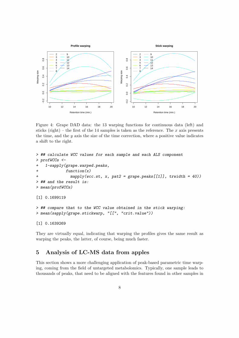
Luckily, we can use one of the big advantages of parametric time warping here, viz.the existance of an explicit warping function. This means we can directly warp thecontinuous profiles using the warping function obtained from the sticks. The result canthen be compared with the result of the warping of the continuous profiles. In Figure 4this is done, with the warping functions of the continuous data on the left, and those ofthe sticks on the right. Clearly, both sets of warping functions are extremely similar. Wecan warp the peaks with both sets of warping functions, and compare the WCC values:

> ## warp peaks according to continuous warping functions

> grape.warped.peaks <-

+ lapply(2:length(grape.peaks),

+ function(ii)

+ lapply(grape.peaks[[ii]],

+ function(x) {

+ new.times <- warp.time(x[,"rt"],

+ t(grape.profwarp[[ii-1]]$warp.coef))

+ x[,"rt"] <- new.times

+ x}))

7

10 12 14 16 18 20

−0.

20.

00.

20.

40.

60.

8Profile warping

Retention time (min.)

War

ping

siz

e

2345678

91011121314

10 12 14 16 18 20

−0.

20.

00.

20.

40.

60.

8

Stick warping

Retention time (min.)

War

ping

siz

e

2345678

91011121314

Figure 4: Grape DAD data: the 13 warping functions for continuous data (left) andsticks (right) – the first of the 14 samples is taken as the reference. The x axis presentsthe time, and the y axis the size of the time correction, where a positive value indicatesa shift to the right.

> ## calculate WCC values for each sample and each ALS component

> profWCCs <-

+ 1-sapply(grape.warped.peaks,

+ function(x)

+ mapply(wcc.st, x, pat2 = grape.peaks[[1]], trwidth = 40))

> ## and the result is:

> mean(profWCCs)

[1] 0.1699119

> ## compare that to the WCC value obtained in the stick warping:

> mean(sapply(grape.stickwarp, "[[", "crit.value"))

[1] 0.1639269

They are virtually equal, indicating that warping the profiles gives the same result aswarping the peaks, the latter, of course, being much faster.

5 Analysis of LC-MS data from apples

This section shows a more challenging application of peak-based parametric time warp-ing, coming from the field of untargeted metabolomics. Typically, one sample leads tothousands of peaks, that need to be aligned with the features found in other samples in

8

Retention time (s)

800 1000 1200 1400 1600 1800 2000

Brookfield

Buby Gala

Buckeye

Fendela de Carli

Galaxy

Incognito

QC

Schniga Ve

STDmix

Figure 5: TICs of the LC-MS data – intensities increase from white to brown to yellow togreen. Injection classes are shown separately to show the gradual increase in retentiontimes more clearly. The earliest injections are at the bottom of each class panel –retention time shifts are up to one minute in size.

order to draw any conclusions. A peak is defined by three characteristics: the retentiontime, the mass-to-charge ratio, and the intensity. All three are subject to experimen-tal error, but the error in retention time is by far the largest and most important, inparticular when comparing data that have not been measured in the same batch.

To align peaks, we start by defining m/z bins of a specific width, and construct apeak list for each bin. The result is very similar in structure to the ALS componentsseen with the DAD data, only more extensive: one can easily define hundreds or eventhousands of bins. Choosing a high resolution leads to many bins, but there will be manycases where bins are empty, or contain only very few peaks. Putting all m/z values in onebin corresponds to something like aligning using the total ion current (TIC), somethingthat is not going to be easy [Bloemberg et al., 2010]. On the other hand, having toofew peaks in individual bins may make the alignment harder because no informationis available for the optimization routine, and one will have to strike a balance betweenthese two effects. Note that this binning process does not mean that mass resolution islost: individual peaks are merely grouped for the purpose of retention time alignment.

The total-ion current (TIC) chromatograms of these data are shown in Figure 5. Toshow the deviations in retention times more clearly, the TICs are shown for each classof apples separately, in order of injection. Note how different the peaks in the standardmixture (at the top of the figure) are, compared to the apple data.

9

5.1 Time warping of QC samples only

For the apple data set, we start by considering only the 27 QC samples. These have beenmeasured at regular intervals, covering the complete injection sequence. First we loadthe data, and define bins of 1 Dalton (i.e., very broad bins) in which peaks are grouped.We only retain those bins containing peaks for at least half the samples.

> QC.idx <- which(metaInf$Variety == "QC")

> QC.pks <- All.pks[QC.idx]

> QC.tics <- All.tics[QC.idx]

> ## divide the peak tables for all files into bins of size 1

> mzbins <- lapply(QC.pks, pktab2mzchannel, massDigits = 0)

> ## which bins occur in more than half of the files?

> allmasses <-

+ table(unlist(lapply(mzbins, function(x) unique(names(x)))))

> mymasses <- as.numeric(names(allmasses[allmasses > 13]))

> length(mymasses)

[1] 698

> ## now we can divide the peak tables again, focusing on these masses only

> QC.mzlist <- lapply(QC.pks, pktab2mzchannel,

+ masses = mymasses, massDigits = 0)

The result is a nested list: for each of the 27 samples, 688 m/z bins are considered indefining a warping function. Clearly, this is much more challenging than the 14 DADsamples with 14 components.

Let us define the first QC sample as the reference sample, and calculate warpingfunctions for all 26 other samples:

> QCwarpings <-

+ lapply(2:length(QC.mzlist),

+ function(ii)

+ stptw(QC.mzlist[[1]], QC.mzlist[[ii]], trwdth = 50))

This step does take some time, so to prevent unnecessary waiting during the developmentof this vignette, we cheat and save intermediate results for later re-use.

We can visualize the effect of the warping by applying it to the (continuous) totalion chromatogram (TIC) data, summarizing for every time point the total amount ofsignal across all masses. Here, we concentrate on the middle part of the chromatogram,between 800 and 2000 seconds:

> ## create a matrix of tic signals from the individual vectors of the

> ## samples - these are not measured at exactly the same times, so we

> ## use interpolation, one value for each second.

> QCticmat <- sapply(QC.tics,

10

800 1000 1200 1400 1600 1800 2000

510

1520

25Original TICs

Retention time (sec.)

QC

sam

ple

800 1000 1200 1400 1600 1800 2000

510

1520

25

Warped TICs

Retention time (sec.)Q

C s

ampl

e

Figure 6: Original TICs of the apple QC samples (left), and TICS warped according tothe warping functions from the peak lists (right). The injection order of the samples isfrom the bottom to the top.

+ function(x)

+ approx(x$scantime, x$tic, tictimes)$y)

> ## Now do the same, but apply the warping to the scantimes

> QCticmat2 <-

+ sapply(seq(along = QC.tics),

+ function(ii) {

+ if (ii == 1) {

+ approx(QC.tics[[ii]]$scantime,

+ QC.tics[[ii]]$tic,

+ tictimes)$y

+ } else {

+ new.times <- warp.time(QC.tics[[ii]]$scantime,

+ QCwarpings[[ii-1]]$warp.coef)

+ approx(new.times, QC.tics[[ii]]$tic, tictimes)$y

+ }})

The result is shown in Figure 6. The left figure clearly shows that peaks elute at latertimes in later QC samples, whereas this trend is absent in the right figure, showing thePTW-corrected TICs.

5.2 Time warping of non-QC samples

Defining the optimal warping works best if the majority of features is present in allsamples. Obviously, in real-life data sets this is very often not the case, and the danger

11

is that the optimization will end up in a suboptimal solution. Two approaches can beused to remedy this. The first assumes that subsequent injections are similar. That is,in finding the optimal warping of sample i+1, one could start from the result of warpingsample i. Not only does this decrease the result of false matches and an incorrect warping,it probably also speeds up the procedure since fewer optimization steps are needed toreach convergence.

However, this is not a fundamental solution to the fact that samples may be verydifferent, and that in such a case false matches between peaks can be expected. Thesecond possibility is to use the QC samples mentioned earlier, and interpolate the warpingfunctions of samples injected between two QC samples. This again assumes a smoothshift in retention times over the injection sequence, which usually is the case. Theretention times of the peaks in the apple samples can then be warped according tothe warping functions found in the QC warping, through a simple process of linearinterpolation between the QCs. We can calculate warped retention times for the QCwarpings and then interpolate, or directly interpolate the warping coefficients:

> interpolate.warping <- function(rt, coef1, coef2, idx,

+ type = c("coef", "time")) {

+ weights <- abs(idx[2:3] - idx[1]) / diff(idx[2:3])

+

+ type <- match.arg(type)

+ if (type == "time") {

+ rt1 <- warp.time(rt, coef1)

+ rt2 <- warp.time(rt, coef2)

+ crossprod(rbind(rt1, rt2), weights)

+ } else {

+ coefs <- crossprod(rbind(coef1, coef2), weights)

+ warp.time(rt, coefs[,1])

+ }

+ }

First we define the relevant QCs for each of the real samples:

> ## sort on injection order

> inj.order <- order(metaInf$InjectionNr)

> metaInf <- metaInf[inj.order,]

> All.pks <- All.pks[inj.order]

> All.tics <- All.tics[inj.order]

> ## pick out only the apple samples

> sample.idx <- which(!(metaInf$Variety %in% c("QC", "STDmix")))

> QC.idx <- which(metaInf$Variety == "QC")

> ## store the IDs of the QC samples around each sample

> neighbours.idx <- t(sapply(sample.idx,

+ function(x) {

+ c(x,

12

+ max(QC.idx[QC.idx < x]),

+ min(QC.idx[QC.idx > x]))

+ }))

> head(neighbours.idx, 9)

[,1] [,2] [,3]

[1,] 7 5 14

[2,] 8 5 14

[3,] 9 5 14

[4,] 10 5 14

[5,] 11 5 14

[6,] 12 5 14

[7,] 13 5 14

[8,] 15 14 21

[9,] 16 14 21

So now we know what warpings to use for each of the sample. For example, let’s lookat the fifth sample, injected at position 12. This is flanked by the fourth and fifth QCsamples, at positions 5 and 14:

> relevant.warpings <- which(QC.idx %in% c(5, 14)) - 1

> ## Original data:

> head(All.pks[[12]][,c("mz", "rt", "maxo", "sn")])

mz rt maxo sn

[1,] 57.06821 1299.491 7.088608 7.150621

[2,] 60.07875 1368.869 12.151901 10.056416

[3,] 67.05031 1370.171 7.088608 5.346768

[4,] 69.06414 1686.200 14.177216 9.407192

[5,] 69.06279 1845.409 14.177216 6.286520

[6,] 69.06596 1616.806 9.113922 4.191239

> ## the weighted average of the warpings of the 2 QC samples

> interpolate.warping(All.pks[[12]][1:6, "rt"],

+ QCwarpings[[relevant.warpings[1]]]$warp.coef,

+ QCwarpings[[relevant.warpings[2]]]$warp.coef,

+ neighbours.idx[5,],

+ type = "time")

[,1]

[1,] 1270.069

[2,] 1338.654

[3,] 1339.941

[4,] 1651.215

[5,] 1807.324

[6,] 1583.025

13

> ## one warping, obtained by the weighted average of the warping coefs

> interpolate.warping(All.pks[[12]][1:6, "rt"],

+ QCwarpings[[relevant.warpings[1]]]$warp.coef,

+ QCwarpings[[relevant.warpings[2]]]$warp.coef,

+ neighbours.idx[5,],

+ type = "coef")

[1] 1270.069 1338.654 1339.941 1651.215 1807.324 1583.025

Clearly, the results of the two types of warping are the same. Calculating averagecoefficients is more efficient, so that is the default in our function. Now, let’s do this forall the samples, where we have to remember not only to correct the retention time butalso the intervals around the retention times:

> corrected.pks <-

+ lapply(1:nrow(neighbours.idx),

+ function(pki) {

+ smp.idx <- which(names(All.pks) ==

+ metaInf[neighbours.idx[pki, 1], "file.name"])

+ QC1 <- which(QC.idx == neighbours.idx[pki, 2]) - 1

+ QC2 <- which(QC.idx == neighbours.idx[pki, 3]) - 1

+

+ coef1 <- QCwarpings[[QC1]]$warp.coef

+ coef2 <- QCwarpings[[QC2]]$warp.coef

+

+ cpk <- All.pks[[smp.idx]]

+ cpk[,"rt"] <- interpolate.warping(cpk[,"rt"],

+ coef1, coef2,

+ neighbours.idx[pki,])

+ cpk[,"rtmin"] <- interpolate.warping(cpk[,"rtmin"],

+ coef1, coef2,

+ neighbours.idx[pki,])

+ cpk[,"rtmax"] <- interpolate.warping(cpk[,"rtmax"],

+ coef1, coef2,

+ neighbours.idx[pki,])

+ cpk

+ })

> names(corrected.pks) <- metaInf[neighbours.idx[,1], "file.name"]

Applying the peak-based warpings to the TICs is done following exactly the same lineas earlier. First we correct all apple profiles:

> samp.tics <- All.tics[sample.idx] ## only real apple samples

> Corr.tics <-

+ lapply(seq(along = samp.tics),

14

Retention time (s)

800 1000 1200 1400 1600 1800 2000

Brookfield

Buby Gala

Buckeye

Fendela de Carli

Galaxy

Incognito

Schniga Ve

Figure 7: Corrected TICs of the LC-MS data, where the warping functions are obtainedfrom the peak lists.

+ function(ii) { ## no warping for the first sample, the reference

+ if (ii == 1) {

+ samp.tics[[1]]

+ } else {

+ QC1 <- which(QC.idx == neighbours.idx[ii, 2]) - 1

+ QC2 <- which(QC.idx == neighbours.idx[ii, 3]) - 1

+

+ coef1 <- QCwarpings[[QC1]]$warp.coef

+ coef2 <- QCwarpings[[QC2]]$warp.coef

+

+ new.times <- interpolate.warping(samp.tics[[ii]]$scantime,

+ coef1, coef2,

+ neighbours.idx[ii,])

+ list(tic = samp.tics[[ii]]$tic, scantime = new.times)

+ }})

A part of the time axis of these corrected TICs is shown in Figure 7. This figure shouldbe compared with Figure 5 – again, we can see that within each class the retention timeshift has been corrected very well. There still is some variation, but the large effects ofthe leaking column have been eliminated, and the remaining variation is probably smallenough to be tackled with the usual retention time correction methods present in XCMS.

15

6 Discussion

Alignment can be a lengthy process, especially when many samples with many timepoints need to be corrected. PTW has always been quite fast, but the new peak-basedform decreases computation times by an order of magnitude or more, which significantlyenhances its usefulness in modern high-throughput applications. The new functionalitycould even be used to fit higher-order warping functions with optimization routines thatare less likely to end up in local minima (but that need more iterations) – in some cases,we have seen that higher-order warping coefficients can be quite variable, and this effectis significantly reduced when using optimization methods like simulated annealing orgenetic algorithms. In practice, this functionality may not be of crucial importance, butthe possibility to investigate this is an asset. In the stptw function experimental codehas been included, accessible through the argument nGlobal: this integer indicates thenumber of global searches to be performed (using function nloptr from the package withthe same name, algorithm “NLOPT_GN_CRS2_LM”) prior to the normal steepest-descentoptimization. By default, nGlobal = 0 when the polynomial degree is three or smaller,and nGlobal = 5 when higher-order polynomials are used. Note that this takes quite abit of computing time.

In this vignette we show that the peak-based warpings are very similar to the originalprofile-based ones, and that forward and backward warping modes can both be used foralignment of chromatographic signals. We explicitly indicate how to use interpolatedwarpings, based on QC samples, for aligning real samples, as already indicated in Eilers[2004]. This is a real bonus in cases where samples of a quite different nature need tobe warped: when comparing cases with controls, for example, it may happen that largedifferences in features lead a classical warping astray and that regular shift correctionssuch as DTW or COW, that do not yield functional descriptions of the optimal warpings,cannot be used.

We already mentioned the simple form of the PTW paradigm, requiring the user onlyto choose a polynomial degree and the similarity function. The latter choice is absent inthe peak-based form of PTW, which is only implemented for the WCC criterion (shownto outperform the other criterion, Euclidean distance, in any case – see Bloemberg et al.[2010]). When analysing the peak lists in LC-MS data, it will be necessary to aggregatethe peaks into m/z bins2 of a certain width. This is an extra step that requires someattention from the user. Luckily, the choice of bin width is not crucial. Wider bins leadto more peaks per bin and fewer alignment steps, and are therefore faster; narrow binscontain few peaks, but then there are more bins to process. In general, as long as thereare not too many empty bins, and there is not too much overlap within individual bins,peak-based PTW will have no problems. In this vignette, for example, we have notoptimized the bin width at all.

2For nominal-mass GC data, this step is not even necessary.

16

References

T.G. Bloemberg, J. Gerretzen, H. Wouters, J. Gloerich, H.J.C.T. Wessels, M. van Dael,L.P. van den Heuvel, P.H.C. Eilers, L.M.C. Buydens, and R. Wehrens. Improvedparametric time warping for proteomics. Chemom. Intell. Lab. Syst., 104:65–74, 2010.

T.G. Bloemberg, J. Gerretzen, A. Lunshof, R. Wehrens, and L.M.C. Buydens. Warpingmethods for spectroscopic and spectrometric signal alignment: a tutorial. Anal. Chim.Acta, 781:14–32, 2013.

D. Clifford and G. Stone. Variable penalty dynamic time warping code for aligning massspectrometry chromatograms in R. J. Stat. Softw., 47(8):1–17, 2012.

A. de Juan and R. Tauler. MCR from 2000: progress in concepts and applications. Crit.Rev. Anal. Chem., 36:163–176, 2006.

P.H.C. Eilers. Parametric time warping. Anal. Chem., 76:404–411, 2004.

A. Gonzalez-Beltran, S. Neumann, E. Maguire, P. Rocca-Serra, and S. Sansone. TheRisa R/Bioconductor package: integrative data analysis from experimental metadataand back again. BMC Bioinformatics, 15(Suppl 1):S11, 2015.

C. A. Smith, E. J. Want, G. O’Maille, R. Abagyan, and G. Siuzdak. XCMS: Process-ing mass spectrometry data for metabolite profiling using nonlinear peak alignment,matching, and identification. Anal. Chem., 78:779–787, 2006.

G. Tomasi, F. van den Berg, and C. Andersson. Correlation-optimized warping and dy-namic time warping as preprocessing methods for chromatographic data. J. Chemom.,19:231–241, 2004.

C.P. Wang and T.L. Isenhour. Time-warping algorithm applied to chromatographic peakmatching gas chromatography / Fourier Transform infrared / Mass Spectrometry.Anal. Chem., 59:649–654, 1987.

R. Wehrens, T.G. Bloemberg, and P.H.C. Eilers. Fast parametric time warping of peaklists. Bioinformatics, In press, 2015a. doi: 10.1093/bioinformatics/btv299.

R. Wehrens, E. Carvalho, and P. Fraser. Metabolite profiling in LC-DAD using multi-variate curve resolution: the alsace package for R. Metabolomics, 11:143–154, 2015b.doi: 10.1007/s11306-014-0683-5.

17

7 Technical details

> sessionInfo()

R version 3.2.1 (2015-06-18)

Platform: x86_64-pc-linux-gnu (64-bit)

Running under: Ubuntu 14.04.2 LTS

locale:

[1] LC_CTYPE=en_US.UTF-8 LC_NUMERIC=C

[3] LC_TIME=nl_NL.UTF-8 LC_COLLATE=en_US.UTF-8

[5] LC_MONETARY=nl_NL.UTF-8 LC_MESSAGES=en_US.UTF-8

[7] LC_PAPER=nl_NL.UTF-8 LC_NAME=C

[9] LC_ADDRESS=C LC_TELEPHONE=C

[11] LC_MEASUREMENT=nl_NL.UTF-8 LC_IDENTIFICATION=C

attached base packages:

[1] parallel stats graphics grDevices utils

[6] datasets methods base

other attached packages:

[1] ptw_1.9-11 lattice_0.20-33

[3] metaMS_1.3.5 CAMERA_1.22.0

[5] igraph_0.7.1 xcms_1.42.0

[7] mzR_2.0.0 Rcpp_0.11.3

[9] Biobase_2.26.0 BiocGenerics_0.12.1

loaded via a namespace (and not attached):

[1] graph_1.44.1 Formula_1.1-2

[3] cluster_2.0.3 splines_3.2.1

[5] tools_3.2.1 nnet_7.3-10

[7] grid_3.2.1 latticeExtra_0.6-26

[9] survival_2.38-3 RBGL_1.42.0

[11] Matrix_1.2-2 nloptr_1.0.4

[13] RColorBrewer_1.1-2 acepack_1.3-3.3

[15] codetools_0.2-11 rpart_4.1-10

[17] robustbase_0.92-3 DEoptimR_1.0-2

[19] Hmisc_3.14-6 stats4_3.2.1

[21] foreign_0.8-65

18