1

Parametric Surface Modeling and

Registration for Comparison of Manual and

Automated Segmentation of the Hippocampus

Li Shen1,2,*, Hiram A. Firpi1, Andrew J. Saykin1, John D. West1

1IU Center for Neuroimaging, Div. of Imaging Sciences, Dept. of Radiology

2Center for Computational Biology and Bioinformatics

Indiana University School of Medicine, 950 W Walnut St., R2 E124, Indianapolis, IN 46202

* Email: shenli@iupui.edu, phone: 317 278 0498, fax: 317 274 1067

Running head: Comparison of Manual and Automated Segmentation of the Hippocampus

Keywords: Shape analysis, segmentation, registration, hippocampus

18 text pages, 7 figures and 1 table

This is the pre-peer reviewed version of the following article: Parametric surface modeling and registration for comparison of manual and automated segmentation of the hippocampus by Shen L, Firpi HA, Saykin AJ, West JD, Hippocampus, 19(6):588-595, 2009, which has been published in final form at http://www3.interscience.wiley.com/journal/122363691/abstract. Hippocampus 19(6) (2009) 588-595 ISSN: 1050-9631 Wiley-Blackwell DOI: 10.1002/hipo.20613 .

2

ABSTRACT

Accurate and efficient segmentation of the hippocampus from brain images is a challenging

issue. Although experienced anatomic tracers can be reliable, manual segmentation is a time

consuming process and may not be feasible for large-scale neuroimaging studies. In this paper,

we compare an automated method, FreeSurfer (V4), with a published manual protocol on the

determination of hippocampal boundaries from MRI scans, using data from an existing MCI/AD

cohort. To perform the comparison, we develop an enhanced spherical harmonic processing

framework to model and register these hippocampal traces. The framework treats the two

hippocampi as a single geometric configuration and extracts the positional, orientation and shape

variables in a multi-object setting. We apply this framework to register manual tracing and

FreeSurfer results together and the two methods show stronger agreement on position and

orientation than shape measures. Work is in progress to examine a refined FreeSurfer

segmentation strategy and an improved agreement on shape features is expected.

INTRODUCTION

The hippocampus has been extensively studied with neuroimaging techniques given its

importance in learning and memory and its potential as a biomarker for brain disorders such as

Alzheimer's disease (Csernansky et al., 2005; Saykin et al., 2006; Thompson et al., 2004; Wang

et al., 2007), epilepsy (Hogan et al., 2006) and schizophrenia (Csernansky et al., 2002; Gerig et

al., 2001; Shenton et al., 2002). While some groups used automated methods for quantification

of the size and shape of the hippocampus (Csernansky et al., 2002; Csernansky et al., 2005;

Hogan et al., 2006; Shen et al., 2002; Wang et al., 2007), in many studies (Gerig et al., 2001;

3

McHugh et al., 2007; Saykin et al., 2006; Shenton et al., 2002; Thompson et al., 2004;

Yushkevich et al., 2007), hippocampal segmentation from magnetic resonance imaging (MRI)

scans was done manually by anatomic tracers using software tools that were either in-home made

or publicly available (e.g., BRAINS (Iowa Mental Health Clinical Research Center, 2008), 3D

Slicer (NAMIC, 2008), ITK-SNAP (Yushkevich et al., 2006)). Many of these tools provide

manual tracing capabilities and semi-automatic approaches involving less human interaction.

Accurate and efficient segmentation of the hippocampus from brain images is still a challenging

issue. Although experienced anatomic tracers can be reliable, manual segmentation is a time

consuming process and may not be feasible for large-scale neuroimaging studies. For example,

the Alzheimer's Disease Neuroimaging Initiative (ADNI) (Mueller et al., 2005) collects 1.5T

structural MRI for over 800 subjects every 6 or 12 months for 2-3 years. Manual segmentation is

apparently not an ideal method for handling such a study involving thousands of MRI scans. A

feasible strategy for hippocampal segmentation in large-scale studies should be able to minimize

human intervention in the processing pipeline. Diffeomorphic mapping is a notable method for

automatic segmentation and has been used by Csernansky and colleagues in many hippocampal

studies (Csernansky et al., 2002; Csernansky et al., 2005; Hogan et al., 2006; Wang et al., 2007).

FreeSurfer (Dale et al., 1999; Fischl et al., 2002; Fischl et al., 1999) is an automatic software tool

for whole brain segmentation and cortical parcellation. Since FreeSurfer is freely available on the

web, it has been widely used in the neuroimaging field. Two recent studies reported similar

results on comparing hippocampal volumes measured using their own manual method and a

specific version of FreeSurfer (V4 in (Shen et al., 2008), V3.04 in (Tae et al., 2008)): the

intraclass correlation coefficients were both between 0.8 and 0.85, showing good agreement.

4

In this paper, we focus on comparing hippocampal morphometric features beyond the volume

determined by the two methods in order to evaluate the reliability of FreeSurfer on extracting

these features. We develop an enhanced spherical harmonic (SPHARM) processing framework

to model and register the hippocampal traces. The framework treats the two hippocampi as a

single configuration and extracts the positional, orientation and shape variables in a multi-object

setting. The proposed registration algorithm operates directly on the SPHARM coefficients and

thus is not only effective but also efficient. We apply this framework to register all the

hippocampal data together and to decouple the position, orientation, and shape for comparing the

manual and FreeSurfer results. The proposed shape modeling and registration framework can

also be used as a general purpose tool for other shape comparison and analysis applications.

MATERIALS AND METHODS

In this work, we use a data cohort for studying memory circuitry in mild cognitive impairment

(MCI) and early Alzheimer's disease (AD). In this MCI/AD cohort, there are hippocampal data

available for 123 subjects total, in four categories: 39 healthy older adults (HC), 38 euthymic

older adults with cognitive complaints (CC) but intact neuropsychological performance, 36 older

adults with amnestic MCI, and 10 adults with AD. Volumetric structural MRI data were acquired

on a 1.5 Tesla GE LX Horizon scanner using a T1-weighted SPGR coronal series with 1.5mm

slice thickness. Further details about this data set are available in (Saykin et al., 2006).

Hippocampal and intracranial boundaries were obtained using (1) a manual protocol reported in

(McHugh et al., 2007) using the BRAINS software package (Iowa Mental Health Clinical

Research Center, 2008), and (2) a fully automated method using the FreeSurfer V4 package

5

(Dale et al., 1999; Fischl et al., 2002; Fischl et al., 1999). For manual segmentation, images were

reformatted into isotropic 1-mm voxels and resampled into the plane perpendicular to the long

axis of the hippocampus using BRAINS. Manual traces were performed in the coronal plane

using markings placed in the axial and sagittal views to guide boundary determination. A 3D

binary image was reconstructed from each set of 2D traces. Further details about this manual

protocol are available in (McHugh et al., 2007). For automated segmentation, FreeSurfer was

employed to automatically label subcortical tissue classes using an atlas-based Bayesian

segmentation procedure (Fischl et al., 2002). We ran the complete FreeSurfer pipeline without

any manual intervention on an IBM HS21 Bladeserver cluster running Red Hat Linux. Each slice

of segmentation label map was inspected by a technician and passed a basic test of quality

control. From each label map, we extracted the left and right hippocampi as two 3D binary

images. Fig. 1 shows sample manual and Freesurfer results. For convenience, we use MT to

indicate the manual tracing method and FS to indicate the FreeSurfer method.

We recently compared hippocampal volume determined by the MT and FS methods (Shen et al.,

2008). Since regional differences in shape are more likely to reveal clues to pathophysiology

than volume, it is critical to examine differences in extracted shape features using various

methods. This paper is focused on examining these morphometric features. We employ the

spherical harmonic (SPHARM) description (Brechbuhler et al., 1995) to model the hippocampal

surfaces and develop an enhanced SPHARM registration algorithm to facilitate the comparison

between the MT and FS data. This method is designed for comparing segmentation methods

performed in two different image spaces (e.g., in our MT and FS cases) without knowing their

6

spatial relationship. If this relationship is known, these two spaces can be easily registered

together and direct 3D volume comparison as proposed in (Fischl et al., 2002) can be applied.

SPHARM (Brechbuhler et al., 1995) is a highly promising surface modeling method that has

been successfully applied to numerous applications in brain imaging. SPHARM is used in this

study for modeling all the hippocampal surfaces. Its first step is to create a continuous and

uniform mapping from the object surface to the surface of a unit sphere. The result is a bijective

mapping between each point v on a surface and a pair of spherical coordinates θ and :

Tzyxv )),(),,(),,((),( . The object surface can then be expanded into a complete set of

spherical harmonic basis functions mlY , where m

lY denotes the spherical harmonic of degree l and

order m. The expansion takes the form: ),(),(0

mll

l

lm

ml Ycv

, where

Tmlz

mly

mlx

ml cccc ),,( . The coefficients m

lc can be estimated up to a user-desired degree by

solving a set of linear equations. The object surface can be reconstructed using these coefficients,

and using more coefficients leads to a more detailed reconstruction (Fig. 2). The degree one

reconstruction is always an ellipsoid. We call it the first order ellipsoid (FOE).

Surface registration aims to register all the models into a common reference system to facilitate

shape comparison. It creates a normalized geometric representation to describe the shape after

normalizing the size, position and orientation measures (i.e., excluding scaling, translation, and

rotation). Since the relative position and orientation between the two hippocampi (or the pose of

the hippocampal pair) are of our interest, we treat the two hippocampi as a single configuration

and study SPHARM registration in a multi-object setting. Scaling invariance can be achieved by

multiplying the coefficients by a scaling factor to normalize a certain volume. We normalize the

7

intracranial volume (ICV) to account for the brain size variation: (1) the mean ICV (= 1421.2

cm3) of the MT data is calculated, and (2) each hippocampal pair in both MT and FS data is

scaled proportionally along with the corresponding ICV so that the ICV is normalized to 1421.2

cm3. While ignoring the degree zero coefficient results in translation invariance for a single

SPHARM model, in our multi-object setting, new methods need to be developed to preserve the

relative position among objects while removing the global translation effect. The surface

registration methods described below aim to remove the effects of global translation and global

rotation for aligning two multi-object complexes together.

The correspondence between SPHARM models is implied by the underlying parameterization:

two points with the same parameter pair (θ,) on two surfaces are defined to be a corresponding

pair. To register multi-object complexes, traditional methods (Shen et al., 2004; Styner et al.,

2006) rotate the parameter net of each individual model to a canonical position on its FOE for

establishing the surface correspondence (Fig. 3), and then use the rigid-body Procrustes method

to align reconstructed surface samples. These methods work well only if the FOE is a real

ellipsoid (e.g., hippocampal case) but not an ellipsoid of revolution or a sphere. To remove this

restriction, we developed a registration method by minimizing the root mean squared distance

(RMSD) between two SPHARM models instead of aligning the FOEs (Shen et al., 2007). Here,

we extend this work to handle multi-object complexes.

Our approach shares a similar idea with the iterative closest point (ICP) method (Besl and

McKay, 1992). We start with an initial alignment and alternately run the following two steps to

refine the alignment until it converges: (1) object space registration for aligning corresponding

surface parts, and (2) parameter space registration for refining the surface correspondence.

8

Suppose that we want to register a multi-object complex X to an atlas A. To create an initial

alignment, we can first align X to A in the object space and then rotate the parameter net of each

SPHARM model in X to best match its counterpart in A. In hippocampal cases, the initial

alignment can be established by applying the FOE method. In cases where the FOE method does

not apply, we can use ICP for initial alignment (see (Shen et al., 2007)).

In object space registration, we aim to improve the alignment in the object space. Since an initial

surface correspondence has been created, we can simply create corresponding surface samples

between X and A and then align two corresponding point sets in a least squares sense (Besl and

McKay, 1992). We call this method as CPS (i.e., aligning corresponding point sets). Let T be the

vector that translates the X center to the A center, and R be the rotation matrix returned by CPS.

We use the following approach to apply T and R to each SPHARM model X and derive a new

SPHARM representation that matches A. Let ),(),(0

mll

l

lm

ml Ycv

be a

SPHARM model. After applying translation T and rotation R, the new coefficients ),( RTcml can

be calculated as follows: (1) 2),( 00

00 TcRTc , and (2) m

lml cRRTc ),( for l,m>0.

In parameter space registration, we aim to improve the surface correspondence between

SPHARM models that are roughly aligned in the object space. Since the underlying

parameterization defines the correspondence between different SPHARM surfaces, our task is to

rotate the parameterization of one model to best match the other's. The goodness of the match is

measured by the root mean squared distance (RMSD) between two models. RMSD can be

calculated directly from SPHARM coefficients. Let S1 and S2 be two SPHARM surfaces, where

their SPHARM coefficients are formed by mlc ,1 and m

lc ,2 , respectively, for 0 ≤ l ≤ lmax and –l ≤ m ≤

9

l. The RMSD between S1 and S2 can be calculated as: 2,2,1

max

0||||)4/(1 m

lm

l

L

l

l

lmccRMSD

. We

employ a sampling-based strategy that fixes one parameterization and rotates the other to

optimize the surface correspondence by minimizing the RMSD. The rotation space can be

sampled nearly uniformly using icosahedron subdivisions. A naive solution for rotating the

parameterization of a SPHARM model is to recalculate the coefficients using the rotated

parameterization. However, it requires solving three linear systems and is time-consuming. To

accelerate the process, we use a rotational property in the harmonic theory and rotate SPHARM

coefficients without recalculating the expansion. Details are available in (Shen et al., 2007).

While traditional registration methods (Shen et al., 2004; Styner et al., 2006) derive sampled

point distribution models as results, our algorithm operates directly on the SPHARM coefficients

and so the results are still SPHARM models. This leads to a better potential of enhancing the

registration results in addition to having a capability of performing subsequent analyses in both

spatial and frequency domains. Fig. 4 shows a sample registration procedure, and we can see that

our algorithm can further improve the FOE registration result with a reduced RMSD.

RESULTS

We compared hippocampal volume between the MT and FS data in (Shen et al., 2008). In this

work, we aim to examine additional morphometric features. Thus, we first exclude volume from

all the MT and FS data: Each hippocampal pair is scaled proportionally along with the

corresponding ICV so that the ICV is normalized to 1421.2 cm3 (i.e., the mean ICV of the MT

data). The subsequent analyses are performed on the data after this scaling normalization.

Atlas Generation and Data Registration

10

We first use all the healthy controls (n=39) in the MT data to create an atlas that represents an

average hippocampal pair. Our method is as follows: (1) let the atlas be the first hippocampal

pair; (2) register each pair to the atlas; (3) let the atlas be the mean of all the data; (4) repeat (2)

and (3) until the atlas converges. The left side of the atlas is shown in Fig. 4(a).

Our overall strategy for aligning the MT and FS data together is as follows: (1) register all the

MT data to the atlas; and (2) register each hippocampal pair in the FS data to its counterpart in

the MT data. We consider two types of registration: a global one and a local one (Styner et al.,

2006). In global registration, we directly apply the algorithm proposed in the Methods Section

for aligning multi-object complexes. This rigid-body algorithm excludes only global translation

and rotation and so the spatial relation between the two hippocampi or the pose of the

hippocampal pair is preserved. In local registration, each individual hippocampus is allowed to

match its template separately. This method expects to derive a better RMSD by allowing local

translation and rotation and may account for possible non-rigid-body transformation effects.

We use RMSD to measure the registration error between an individual and its template. Fig. 5

shows sample global and local registration results for the MT and FS hippocampal traces of a

same subject. While both methods can derive good registration results, the local method does

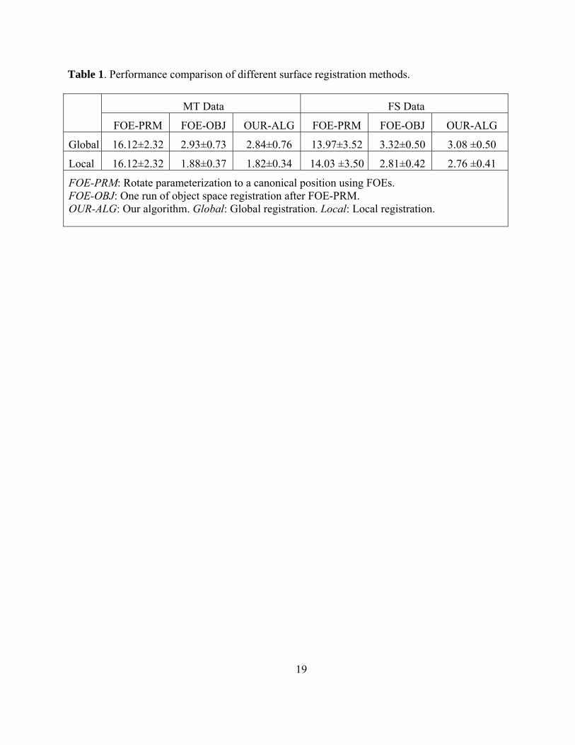
generate better RMSDs. Table 1 shows a comparison of applying various registration methods

on the MT and FS data, where each entry records (mean±std) of the registration errors for all

subjects in a particular data set by a certain method. For either of global and local strategies, we

compare three methods: (1) FOE-PRM: rotating parameterization to a canonical position using

FOEs, (2) FOE-OBJ: one run of object space registration after FOE-PRM, and (3) OUR-ALG:

our algorithm proposed above. Although the traditional SPHARM registration methods work

11

well on hippocampal data (see the FOE-OBJ columns for their results), our algorithm is able to

further improve these results (see the OUR-ALG columns).

Position, Orientation and Shape

While global registration excludes global effects on translation and rotation, the spatial

relationship between the two hippocampi is preserved. We use the globally registered FOE

model to define this local pose information, including the position and orientation of each

hippocampus. Let h be a hippocampus, SPh be its SPHARM model that is registered in the atlas

space, Ph be the FOE center of SPh, and Nh be the FOE north pole of SPh (see Fig. 3 for sample

FOEs on which north poles are shown as yellow dots). We define Ph to be the position measure

of h and Oh = (Nh-Ph) / |Nh-Ph| to be the orientation measure of h.

We report our work on comparing the position and orientation measures determined by the MT

and FS methods. We use the position measure of the left hippocampus as an example to show

our approach. Let S be our subject set. Given xS, we use Mxl to denote its left hippocampus

determined by the M method, where M{MT, FS}. We start with a simple examination of three

sets of position distances: (1) intra-subject distances between the MT and FS methods:

Dmtfs={ || FSx

MTx ll

PP | xS}; (2) inter-subject distances within the MT data: Dmtmt={ || MTy

MTx ll

PP |

x,yS, x≠y}; and (3) inter-subject distances within the FS data: Dfsfs={ || FSy

FSx ll

PP | x,yS, x≠y}.

Similar calculations are applied to the right hippocampus and the orientation measures. The

orientation distance is measured by the angle between two directions.

12

Fig. 6 shows the distributions of all these distance collections. The MT and FS methods show

good agreement on position measures: The intra-subject distances between the two methods

(Dmtfs, top row) are narrowly distributed and close to zeros, compared with large inter-subject

variations shown in both MT data (Dmtmt, middle row) and FS data (Dfsfs, bottom row). As to

orientation, the intra-subject distances between the two methods (top row) are similar to the

inter-subject distances within either of the methods (middle and bottom rows). All these

distances are small, suggesting a consistent similarity in relative orientations between two

hippocampi. For local registration, we did the same experiments, and all the distances on

position or orientation measures became zero. This indicates that local registration excludes both

global and local translation and rotation effects of each individual hippocampus.

Finally we examine the shape measures. Since we have established surface correspondence

among SPHARM models, given any two models, we can calculate a distance map showing the

model difference on each surface location. Similar to the position and orientation cases, we

calculate three sets of distance maps: (1) intra-subject distances between MT and FS methods,

(2) inter-subject distances within the MT data, and (3) inter-subject distances within the FS data.

Since it is hard to visualize the distance distribution for all the surface locations, we only show

the mean and standard deviation of these distance maps in Fig. 7. For global registration,

compared with the inter-subject distances within a method (MT or FS, see middle or bottom

row), the intra-subject distances between two methods (top row) are relatively small. This

indicates some degree of agreement, but it might be related only to position and orientation

factors, since globally registered models contain not only shape but also position and orientation

information. In local registration, the position and orientation information is excluded, and the

13

intra-subject distances between the methods (top row) and the inter-subject distances within the

method (middle and bottom rows) become at a similar level. To make the two methods agree

more on shape, it appears there is still room for improvement. In particular, the tail region shows

a notable systematic difference. By a visual inspection of the raw data (Fig. 1), we notice that the

FS results tend to have a fatter tail and some noisy spikes on the surface.

DISCUSSION

We have compared FreeSurfer (V4) with a published manual protocol on the determination of

hippocampal boundaries from MRI scans, using data from an existing MCI/AD cohort. This

comparison is enabled by an improved SPHARM modeling and registration procedure. We use a

global registration process to extract relative position and orientation measures of the two

hippocampi, and the manual and FreeSurfer methods show good agreement on these measures.

We use a local registration process to account for possible non-rigid-body transformation effects

and extract fine-scale surface shape measures, and the two methods show less agreement on

these measures. Visual inspection of raw data shows the FreeSurfer results tend to have a fatter

tail and some noisy spikes on the surface. We plan to examine a refined FreeSurfer segmentation

strategy and expect an improved agreement on shape features. Other interesting future topics

include: (1) Can the results be greatly improved by involving minimal human intervention? (2)

Are the discriminative powers to detect disease similar between the manual and FreeSurfer data?

REFERENCES

Besl PJ, McKay ND. 1992. A method for registration of 3-D shapes. IEEE Trans. on Pattern

Analysis and Machine Intelligence 14(2):239-256.

14

Brechbuhler C, Gerig G, Kubler O. 1995. Parametrization of closed surfaces for 3D shape

description. Computer Vision and Image Understanding 61(2):154-170.

Csernansky JG, Wang L, Jones D, Rastogi-Cruz D, Posener JA, Heydebrand G, Miller JP, Miller

MI. 2002. Hippocampal deformities in schizophrenia characterized by high dimensional

brain mapping. Am J Psychiatry 159(12):2000-6.

Csernansky JG, Wang L, Swank J, Miller JP, Gado M, McKeel D, Miller MI, Morris JC. 2005.

Preclinical detection of Alzheimer's disease: hippocampal shape and volume predict

dementia onset in the elderly. Neuroimage 25(3):783-92.

Dale AM, Fischl B, Sereno MI. 1999. Cortical surface-based analysis. I. Segmentation and

surface reconstruction. Neuroimage 9(2):179-94.

Fischl B, Salat DH, Busa E, Albert M, Dieterich M, Haselgrove C, van der Kouwe A, Killiany R,

Kennedy D, Klaveness S and others. 2002. Whole brain segmentation: automated

labeling of neuroanatomical structures in the human brain. Neuron 33(3):341-55.

Fischl B, Sereno MI, Dale AM. 1999. Cortical surface-based analysis. II: Inflation, flattening,

and a surface-based coordinate system. Neuroimage 9(2):195-207.

Gerig G, Styner M, Shenton ME, Lieberman JA. Shape versus size: Improved understanding of

the morphology of brain structures. Lecture Notes in Computer Science; 2001 Oct. 14–

17; Ultrecht, the Netherlands. Springer. p 24–32.

Hogan RE, Wang L, Bertrand ME, Willmore LJ, Bucholz RD, Nassif AS, Csernansky JG. 2006.

Predictive value of hippocampal MR imaging-based high-dimensional mapping in mesial

temporal epilepsy: preliminary findings. AJNR Am J Neuroradiol 27(10):2149-54.

15

Iowa Mental Health Clinical Research Center. 2008. BRAINS Software Package. Available at

http://www.psychiatry.uiowa.edu/mhcrc/IPLpages/BRAINS.htm.

McHugh TL, Saykin AJ, Wishart HA, Flashman LA, Cleavinger HB, Rabin LA, Mamourian

AC, Shen L. 2007. Hippocampal volume and shape analysis in an older adult population.

Clin Neuropsychol 21(1):130-45.

Mueller SG, Weiner MW, Thal LJ, Petersen RC, Jack C, Jagust W, Trojanowski JQ, Toga AW,

Beckett L. 2005. The Alzheimer's disease neuroimaging initiative. Neuroimaging Clin N

Am 15(4):869-77, xi-xii.

NAMIC. 2008. 3D Slicer Web Page. Available at http://www.slicer.org.

Saykin AJ, Wishart HA, Rabin LA, Santulli RB, Flashman LA, West JD, McHugh TL,

Mamourian AC. 2006. Older adults with cognitive complaints show brain atrophy similar

to that of amnestic MCI. Neurology 67:834-842.

Shen D, Moffat S, Resnick SM, Davatzikos C. 2002. Measuring size and shape of the

hippocampus in MR images using a deformable shape model. Neuroimage 15(2):422-34.

Shen L, Huang H, Makdeon F, Saykin AJ. 2007. Efficient Registration of 3D SPHARM

Surfaces. CRV 2007. Montreal, QC.

Shen L, Makedon F, Saykin AJ. 2004. Shape-based discriminative analysis of combined bilateral

hippocampi using multiple object alignment. SPIE Proc. 5370. p 274–282.

Shen L, Saykin AJ, Firpi HA, West JD, McHugh TL, and others. 2008. Comparison of manual

and automated determination of hippocampal volumes in MCI and older adults with

cognitive complaints. Alzheimer's & Dementia 4(4):Suppl 2:T29-30.

16

Shenton ME, Gerig G, McCarley RW, Szekely G, Kikinis R. 2002. Amygdala-hippocampal

shape differences in schizophrenia: the application of 3D shape models to volumetric MR

data. Psychiatry Res 115(1-2):15-35.

Styner M, Gorczowski K, Fletcher T, Jeong JY, Pizer SM, Gerig G. 2006. Multi-Object Statistics

using Principal Geodesic Analysis in a Longitudinal Pediatric Study. LNCS 4091. p 1-8.

Tae WS, Kim SS, Lee KU, Nam EC, Kim KW. 2008. Validation of hippocampal volumes

measured using a manual method and two automated methods (FreeSurfer and IBASPM)

in chronic major depressive disorder. Neuroradiology.

Thompson PM, Hayashi KM, De Zubicaray GI, Janke AL, Rose SE, Semple J, Hong MS,

Herman DH, Gravano D, Doddrell DM and others. 2004. Mapping hippocampal and

ventricular change in Alzheimer disease. Neuroimage 22(4):1754-66.

Wang L, Beg F, Ratnanather T, Ceritoglu C, Younes L, Morris JC, Csernansky JG, Miller MI.

2007. Large deformation diffeomorphism and momentum based hippocampal shape

discrimination in dementia of the Alzheimer type. IEEE Trans Med Im 26(4):462-70.

Yushkevich PA, Detre JA, Mechanic-Hamilton D, Fernandez-Seara MA, Tang KZ, Hoang A,

Korczykowski M, Zhang H, Gee JC. 2007. Hippocampus-specific fMRI group activation

analysis using the continuous medial representation. Neuroimage 35(4):1516-30.

Yushkevich PA, Piven J, Hazlett HC, Smith RG, Ho S, Gee JC, Gerig G. 2006. User-guided 3D

active contour segmentation of anatomical structures: significantly improved efficiency

and reliability. Neuroimage 31(3):1116-28.

ACKNOWLEDGEMENTS

17

Supported in part by NIBIB/NEI R03 EB008674-01, NIA R01 AG19771, NCI R01 CA101318

and U54 EB005149 from the NIH, Foundation for the NIH, and grant #87884 from the Indiana

Economic Development Corporation (IEDC). We thank Nick Schmansky and Bruce Fischl of

Harvard Medical School and Randy Heiland of Indiana University for help with running

FreeSurfer on IU's supercomputers.

TABLE AND FIGURE LEGENDS

Table 1. Performance comparison of different surface registration methods.

Fig. 1. Sample segmentation results generated by manual tracing (left) and FreeSurfer (right):

Each hippocampus is described by a binary image and the corresponding voxel surface is

displayed. Left hippocampi are shown in green and right in red.

Fig. 2. Sample SPHARM reconstructions: Shown from left to right are original surface and

SPHARM reconstructions up to degrees 1, 5 and 15.

Fig. 3. Using first order ellipsoids (FOEs) to establish surface correspondence between two

subjects: Each row corresponds to one subject, where both FOEs and the degree 15 SPHARM

reconstructions are displayed. The underlying parameterization defines the correspondence

between SPHARM models and is shown as a colorful mesh superimposed onto the surface.

Shown in (a) is the initial configuration of each subject, where the parameter nets are not aligned

well. Shown in (b) is the result of rotating the FOEs to a canonical position to establish surface

correspondence across subjects.

18

Fig. 4. Sample registration procedure: (a) The atlas. (b) The initial configuration of an individual,

where the surface correspondence to the atlas has been established by FOE. (c) Result of object

space registration. (d) Result of parameter space registration. RMSD (in mm) is shown. The

parameter net is shown as a colorful mesh on the surface.

Fig. 5. Global registration (a) and local registration (b) for a same subject. In each of (a) and (b):

Shown in the first row are (1) the atlas to which the MT model is registered, (2) the initial MT

model, and (3) the registered MT model; and shown in the second row are (4) the MT model to

which the FS model is registered (i.e., the same as (3)), (5) the initial FS model, and (6) the

registered FS model. RMSDs (in mm) are shown. The underlying parameterization is shown as a

colorful mesh on each surface.

Fig. 6. Distributions of intra-subject and inter-subject distances on (a) position measures and (b)

orientation measures after global registration. In each of (a) and (b), the left column shows the

results for the left hippocampi and the right column for the right ones. Shown in the top row are

intra-subject distances between the MT and FS methods, in the middle row inter-subject

distances within the MT data, and in the bottom row inter-subject distances within the FS data.

Fig. 7. Statistical maps of intra-subject and inter-subject surface distances after (a) global

registration or (b) local registration. In each of (a) and (b), the left column shows the mean map,

and the right column shows the standard deviation map. Shown in the top row are intra-subject

distances between the MT and FS methods, in the middle row inter-subject distances within the

MT data, and in the bottom row inter-subject distances within the FS data. All the mean and

standard deviation maps are color-coded and superimposed onto the hippocampal atlas.

19

Table 1. Performance comparison of different surface registration methods.

MT Data FS Data

FOE-PRM FOE-OBJ OUR-ALG FOE-PRM FOE-OBJ OUR-ALG

Global 16.12±2.32 2.93±0.73 2.84±0.76 13.97±3.52 3.32±0.50 3.08 ±0.50

Local 16.12±2.32 1.88±0.37 1.82±0.34 14.03 ±3.50 2.81±0.42 2.76 ±0.41

FOE-PRM: Rotate parameterization to a canonical position using FOEs. FOE-OBJ: One run of object space registration after FOE-PRM. OUR-ALG: Our algorithm. Global: Global registration. Local: Local registration.

20

Fig. 1. Sample segmentation results generated by manual tracing (left) and FreeSurfer (right):

Each hippocampus is described by a binary image and the corresponding voxel surface is

displayed. Left hippocampi are shown in green and right in red.

21

Fig. 2. Sample SPHARM reconstructions: Shown from left to right are original surface and

SPHARM reconstructions up to degrees 1, 5 and 15.

22

Fig. 3. Using first order ellipsoids (FOEs) to establish surface correspondence between two

subjects: Each row corresponds to one subject, where both FOEs and the degree 15 SPHARM

reconstructions are displayed. The underlying parameterization defines the correspondence

between SPHARM models and is shown as a colorful mesh superimposed onto the surface.

Shown in (a) is the initial configuration of each subject, where the parameter nets are not aligned

well. Shown in (b) is the result of rotating the FOEs to a canonical position to establish surface

correspondence across subjects.

23

Fig. 4. Sample registration procedure: (a) The atlas. (b) The initial configuration of an individual,

where the surface correspondence to the atlas has been established by FOE. (c) Result of object

space registration. (d) Result of parameter space registration. RMSD (in mm) is shown. The

parameter net is shown as a colorful mesh on the surface.

24

Fig. 5. Global registration (a) and local registration (b) for a same subject. In each of (a) and (b):

Shown in the first row are (1) the atlas to which the MT model is registered, (2) the initial MT

25

model, and (3) the registered MT model; and shown in the second row are (4) the MT model to

which the FS model is registered (i.e., the same as (3)), (5) the initial FS model, and (6) the

registered FS model. RMSDs (in mm) are shown. The underlying parameterization is shown as a

colorful mesh on each surface.

26

Fig. 6. Distributions of intra-subject and inter-subject distances on (a) position measures and (b)

orientation measures after global registration. In each of (a) and (b), the left column shows the

results for the left hippocampi and the right column for the right ones. Shown in the top row are

intra-subject distances between the MT and FS methods, in the middle row inter-subject

distances within the MT data, and in the bottom row inter-subject distances within the FS data.

27

Fig. 7. Statistical maps of intra-subject and inter-subject surface distances after (a) global

registration or (b) local registration. In each of (a) and (b), the left column shows the mean map,

and the right column shows the standard deviation map. Shown in the top row are intra-subject

distances between the MT and FS methods, in the middle row inter-subject distances within the

MT data, and in the bottom row inter-subject distances within the FS data. All the mean and

standard deviation maps are color-coded and superimposed onto the hippocampal atlas.