Parametric representation of the cloud droplet spectra … · 1Royal Netherlands Meteorological Institute (KNMI), De Bilt, The Netherlands ... (CDSD), the parameterized microphysical

Atmos. Chem. Phys., 10, 4835–4848, 2010www.atmos-chem-phys.net/10/4835/2010/doi:10.5194/acp-10-4835-2010© Author(s) 2010. CC Attribution 3.0 License.

AtmosphericChemistry

and Physics

Parametric representation of the cloud droplet spectra for LESwarm bulk microphysical schemes

O. Geoffroy1, J.-L. Brenguier2, and F. Burnet2

1Royal Netherlands Meteorological Institute (KNMI), De Bilt, The Netherlands2CNRM/GAME (Meteo-France, CNRS), Toulouse, France

Received: 16 July 2009 – Published in Atmos. Chem. Phys. Discuss.: 25 August 2009Revised: 1 February 2010 – Accepted: 3 May 2010 – Published: 26 May 2010

Abstract. Parametric functions are currently used to rep-resent droplet spectra in clouds and to develop bulk param-eterizations of the microphysical processes and of their in-teractions with radiation. The most frequently used para-metric functions are the Lognormal and the GeneralizedGamma which have three and four independent parameters,respectively. In a bulk parameterization, two parameters areconstrained by the total droplet number concentration andthe liquid water content. In the Generalized Gamma func-tion, one parameter is specified a priori, and the fourth one,like the third parameter of the Lognormal function, shall betuned, for the parametric function to statistically best fit ob-served droplet spectra.

These parametric functions are evaluated here usingdroplet spectra collected in non-or slightly precipitating stra-tocumulus and shallow cumulus. Optimum values of the tun-ing parameters are derived by minimizing either the absoluteor the relative error for successively the first, second, fifth,and sixth moments of the droplet size distribution. A trade-off value is also proposed that minimizes both absolute andrelative errors for the four moments concomitantly. Finally, aparameterization is proposed in which the tuning parameterdepends on the liquid water content. This approach signifi-cantly improves the fit for the smallest and largest values ofthe moments.

Correspondence to:O. Geoffroy([email protected])

1 Introduction

Cloud particles are represented by their size distributionalso referred to as spectrum. In the liquid phase, the spec-trum originates from activation of cloud condensation nuclei(CCN), mainly at cloud base. Hence it expends from submi-cron particles for the smallest activated CCNs to about 10 µmin radius for the giant ones. As particles grow by condensa-tion, the spectrum gets narrower because the growth rate of adroplet is inversely proportional to its size. Higher in a cloud,spectral narrowing is counterbalanced by broadening pro-cesses, mainly by turbulent mixing, because particles expe-rience different growth histories along different trajectories,some ascending adiabatically from cloud base, while othersundergo dilution with environmental air and partial evapora-tion. New CCNs can also be activated higher than cloud base,when moist and clear air is entrained in an updraft, henceinitiating small droplets. When the biggest droplets reacha radius of about 20 µm, collision and coalescence generatedrizzle particles (from 20 to a few 100 µm). If the cloud issufficiently deep and the liquid water content large enough,droplets and drops continue to collide to form precipitationdrops (mm). The maximum drop radius, of the order of4 mm, is limited by break-up, either following a collisionor spontaneously for the biggest drops. The total numberconcentration spans over a large range, because millions ofdroplets are necessary to form a drop. It thus evolves from upto 1000 cm−3 for droplets in a polluted environment, to a fewper cubic meter for precipitation drops. Because the numberconcentration of activated CCN, the parcel trajectories, theseries of mixing events and the resulting growth histories bycondensation, collection and break-up are infinitely diverse,cloud particle spectra exhibit all kinds of shapes (Warner,1969a, b, 1970, 1973a, b).

Published by Copernicus Publications on behalf of the European Geosciences Union.

http://creativecommons.org/licenses/by/3.0/

4836 O. Geoffroy et al.: Parametric representation of the cloud droplet spectra

Table 1. Typical bulk parameterizations using two particle categories with, from left to right, the value of the threshold radius between the twocategories, the number of independent variables for the description of the droplet size distribution (CDSD), the parameterized microphysicalprocesses, the methodology adopted for the development of the parametrization, and the CDSD parametric representation.

Number of independentSeparation variables for the Microphysical Methodology&

Reference radiusr0 description of the CDSD processes CDSD hypothesis

Kessler NA qc autoconversion Empirical CDSD:(1969) monodispersed

Manton and Cotton NA qc, Nc autoconversion Analytical CDSD:(1977) monodispersed

Berry and Reinhardt variable, qc, Nc, σ x autoconversion Empirical,∼30(1974) ∼41 µm spectra from 0-D bin

simulations, CDSD: GG3

Khairoutdinov and Kogan 25 µm qc, Nc autoconversion Empirical, 100 000 spectra(2000) from 3-D bin simulations of

Sc, CDSD: GG1

Liu and Daum NA qc,Nc,d autoconversion Analytical,(2004) CDSD: GG1

Seifert and Beheng 41 µm qc, Nc, autoconversion Analytical and empirical,(2001, 2006) νc=ν3−1 GG3 and spectra from 1-D

bin simulations, CDSD: GG3

Cohard and Pinty NA qc, NCCN activation Analytical(2000) CDSD: GG3

Ackerman NA qc, Nc, σg Cloud droplet Analytical(2008) sedimentation CDSD: Lognormal

The cloud droplet size distribution (CDSD) is expressedas a concentration density,n(r)dr, i.e. number density ofdroplets per volume (or per mass) of air, and per unit size.To summarize the properties of a size distribution, one com-monly uses a moment of the distributionMp, or the meanradius of thepth momentrp:

Mp =

∞∫0

rpn(r)dr, (1)

rp =

(Mp

/N

) 1p

(2)

whereN=M0 is the total number concentration.To interpret microphysical observations, examine the in-

teractions between cloud microphysics and other physicalprocesses, and numerically simulate these interactions, para-metric functions are frequently used to reduce the variety ofthe droplet spectral shapes. The objective in this paper isto evaluate parametric functions that best replicate observedspectra on a statistical basis. The focus is on non-or slightlyprecipitating stratocumulus and shallow cumulus clouds.

After a brief description (Sect. 2) of bulk microphysicsschemes, three frequently used parametric functions are de-scribed in Sect. 3. The methodology for tuning the func-tions and the data sets on which tuning relies are detailed in

Sects. 4 and 5, respectively. Section 6 addresses the specificissue of scaling up small scale measurements for character-izing cloud system properties. The results are then reportedin Sect. 7, for fixed and variables values of the tuning param-eters successively, before the conclusions.

2 Bulk parameterizations and parametric functions

In a numerical model, the natural variability of the dropletspectra can be explicitly simulated with “bin” microphysicalschemes where the number distribution is discretized, from30 to 200 size classes (Kogan, 1991). The computationalcost of such schemes however, prevents their use in large do-main, high spatial resolution, cloud resolving models. In-stead, bulk parameterizations have been developed. Indeed,even though spectra are diverse, one usually observe a transi-tion from droplets to drops, in the size range where conden-sational growth becomes inefficient, while collection startsto become significant, namely between 20 and 50 µm in ra-dius. This size range also corresponds to a rapid increaseof the particle fall velocity with the particle radius (∝r2).In a liquid phase bulk scheme, hydrometeors are thus dis-tributed in two categories, the droplets that do not or slowlysediment, and the drops that precipitate more rapidly. This

Atmos. Chem. Phys., 10, 4835–4848, 2010 www.atmos-chem-phys.net/10/4835/2010/

O. Geoffroy et al.: Parametric representation of the cloud droplet spectra 4837

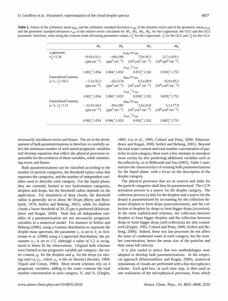
Table 2. Values of the arithmetic mean µabsand the arithmetic standard deviationσabsof the absolute errors and of the geometric meanµreland the geometric standard deviationσ rel of the relative errors calculated forM1, M2, M5, M6, for the Lognormal, the GG1 and the GG3parametric functions, when using the constant trade-off tuning parameters values,σ∗

g for the Lognormal,ν∗1 for the GG1 andν∗

3 for the GG3.

M1 M2 M5 M6

Lognormal, µabs±σabsσ∗

g=1.34 −0.82±31.1 −40±266 7.9±30.3 23.7±103.1(µm cm−3) (µm2 cm−3) (105µm5 cm−3) (106 µm6 cm−3)

µrel×

/ σ rel

1.001×/ 1.054 1.004×/ 1.052 0.972×/ 1.332 0.910×/ 1.751

Generalized Gamma, µabs±σabsα=1, ν∗

1=10.3 −5.3±32.2 −62±274 6.5±28.9 16.9±93.2(µm cm−3) (µm2 cm−3) (105µm5 cm−3) (106µm6 cm−3)

µrel×

/ σ rel

1.002×/ 1.054 1.000×/ 1.052 0.958×/ 1.332 0.870×/ 1.751

Generalized Gamma, µabs±σabsα=3, ν∗

3=1.11 −12.0±34.4 −84±282 3.4±25.8 5.1±77.9(µm cm−3) (µm2 cm−3) (105µm5 cm−3) (106µm6 cm−3)

µrel×

/ σ rel

0.991×/ 1.054 0.996×/ 1.052 0.926×/ 1.332 0.803×/ 1.751

necessarily introduces errors and biases. The art in the devel-opment of bulk parameterizations is therefore to carefully se-lect the minimum number of well suited prognostic variablesand develop equations that reflect the physical processes re-sponsible for the evolution of these variables, while minimiz-ing errors and biases.

Bulk parameterizations can be classified according to thenumber of particle categories, the threshold radius value thatseparates the categories, and the number of independent vari-ables used to describe each category. For the liquid phase,they are currently limited to two hydrometeor categories,droplets and drops, but the threshold radius depends on theapplication. For simulation of deep clouds, the thresholdradius is generally set to about 40–50 µm (Berry and Rein-hardt, 1974; Seifert and Beheng, 2001), while for shallowclouds a lower threshold of 20–25 µm is preferred (Khairout-dinov and Kogan, 2000). Note that all independent vari-ables of a parameterization are not necessarily prognosticvariables in a numerical model. For instance in Seifert andBeheng (2006), using a Gamma distribution to represent thedroplet mass spectrum, the parameterνc is set to 1; in Ack-erman et al. (2008) using a Lognormal distribution, the pa-rameterσ g is set to 1.5, although a value of 1.2 is recog-nized to better fit the observations. Original bulk schemeswere limited to one prognostic variable per category: the wa-ter content,qc for the droplets andqr for the drops (or mix-ing ratio=q/ρa , whereρa is the air density) (Kessler, 1969;Tripoli and Cotton, 1980). More recent schemes rely on 4prognostic variables, adding to the water contents the totalnumber concentration in each category,Nc andNr (Ziegler,

1985; Liu et al., 1995; Cohard and Pinty, 2000; Khairout-dinov and Kogan, 2000; Seifert and Beheng, 2001). Beyondthe total water content and total number concentration of par-ticles in each category, there were a few attempts to introducemore variety by also predicting additional variables such asthe reflectivity, as in Milbrandt and Yau (2005). Table 1 sum-marizes the characteristics of existing bulk parameterizationsfor the liquid phase, with a focus on the description of thedroplet category.

The physical processes that act as sources and sinks forthe particle categories shall then be parameterized. The CCNactivation process is a source for the droplet category. Thecollection process (a sink for the droplets and a source for thedrops) is parameterized by accounting for the collection be-tween droplets to form drops (autoconversion), and the col-lection of droplets by drops to form bigger drops (accretion).In the most sophisticated schemes, the collection betweendroplets to form bigger droplets and the collection betweendrops to form bigger drops (self-collection) are also consid-ered (Ziegler, 1985; Cohard and Pinty, 2000; Seifert and Be-heng, 2006). Indeed, these two last processes do not affectthe mass of condensed water in each category, but the num-ber concentration, hence the mean size of the particles andtheir mean fall velocity.

It is also useful to notice that two methodologies wereadopted to develop bulk parameterizations. In the empiri-cal approach (Khairoutdinov and Kogan, 2000), numericalsimulations of clouds are performed with a bin microphysicsscheme. Each grid box, at each time step, is then used asone realisation of the microphysical processes, from which

www.atmos-chem-phys.net/10/4835/2010/ Atmos. Chem. Phys., 10, 4835–4848, 2010


bulk variables (qc, qr , Nc, Nr) and their evolution rates byCCN activation, autoconversion, accretion, and precipitationcan be calculated. Empirical laws are then derived by min-imization over the whole set of realisations. In such a case,the accuracy of the parameterization is limited by the perfor-mance of the bin microphysics scheme and the variable spaceexplored by the simulations. Others (Liu and Daum, 2004)follow a more analytical approach in which the particle sizedistribution in each category is represented by a parametricfunction. The stochastic collection equation is then analyti-cally resolved to derive a formulation of the autoconversionand accretion rates. In this case the accuracy of the solu-tion mainly depends on the realism of the chosen parametricfunction. Note however, that coefficients of some “analyticaltype” bulk parameterizations are tuned empirically (Seifertand Beheng, 2001, 2006).

Some physical processes in a cloud model require ad-ditional information about cloud microphysics, beyond theprognostic number concentration (N = M0) and water con-tent (∝M3). For instance, CCN activation is often param-eterized using a diagnostic of the peak supersaturation, thatdepends on the first moment of the size distributionM1, alsoreferred to as the droplet integral radius (Twomey, 1959).Radiative transfer calculations in clouds depend on light ex-tinction that is proportional to the second momentM2 ofthe droplet spectrum (Hansen and Travis, 1974). The sedi-mentation flux depends on the droplet sizes, through an ap-proximation of their fall velocity. For particles smaller than30 µm in radius, the terminal fall velocity verifying roughlythe Stokes’ law (Roger and Yau, 1989), the sedimentationflux of particle number is proportional to the second mo-ment, M2, and the sedimentation flux of water content isproportional to the fifth moment,M5. The radar reflectivityin a liquid phase cloud is proportional to M6 (Atlas, 1954).

The width of the size distributionw=1/M0

√M0M2−M2

1 ,or its dispersiond=N ·w/M1, have been used to establish re-lationships between the mean volume and effective radii ofthe droplet spectrum for radiative transfer calculations (Liuand Daum, 2000). It is therefore not sufficient for a micro-physics bulk parameterization to accurately predict the auto-conversion and accretion rates; it must also provide accuratediagnostics of various integral properties of the cloud dropletspectrum, at least forM1, M2, M5, M6.

In summary, bulk parameterizations that are developed fol-lowing an analytical approach rely on a priori specified para-metric functions for the description of the droplet spectra.Moreover, all bulk parameterizations, including those empir-ically tuned, also require a priori specified parametric func-tions to establish formal relationships between the prognos-tic moments of the droplet size distribution (M0 andM3) andthose used in the parameterization of each microphysical pro-cess.

3 Commonly used parametric functions

To represent droplet size distributions, the most frequentlyused parametric functions are the Lognormal (Clark, 1976;Feingold et Levin, 1986) and the Generalized Gamma (Liuand Hallett, 1998; Cohard and Pinty, 2000). These two func-tions are convenient because any of their moments can beexpressed as a function of the parameters of the distribution.The Lognormal function

nc(r) = N1

√2πr lnσg

exp

(−

1

2

(ln(r/rg)

lnσg

)2)

(3)

has 3 independent parameters, the total number concentra-tion N , the geometric standard deviationσ g, and the meangeometric radiusrg, whererg=e<ln(r)>. Thep moment ofthe spectrum is directly related toN , σ g, andrg via:

Mp = Nrpg exp

(p2

2(lnσg)

2

), (4)

and it is expressed as a function ofN , M3 andσ g as

Mp = N1−p/3Mp/33 exp

(p2

−9

2ln(σg)

2

). (5)

The Generalised Gamma function

n(r) = Nα

0(ν)λανrαν−1exp(−(λr)α) (6)

has 4 independent parameters,N , the slope parameterλ andthe two shape parametersα andν. Thepth moment of thespectrum is directly related toN , λ, α andν via:

Mp =N

λp

(0(ν +

pα)

0(ν)

)(7)

and it is expressed as a function ofN , M3, α andν as:

Mp = N1−p/3Mp/33

0(ν +pα)

0(ν +3α)

p30(ν)

p−33 . (8)

The Generalized Gamma function includes the Gamma (orGolovin), the Exponential and the Weibull functions. Indeed,the Gamma function (Liu and Daum, 2004) is a GeneralizedGamma withα=1 (hereafter referred to as GG1). Some au-thors use the Gamma function to represent the cloud dropletmass distribution (Berry and Reinhardt, 1974; Williams andWojtowicz, 1982; Seifert and Beheng, 2001), which is equiv-alent of using a Generalized Gamma function withα=3(hereafter referred to as GG3) for describing the particlenumber concentration distribution. In this paper, both val-ues,α=1 andα=3, are evaluated.

In summary, in the framework of a bulk parameterizationwith two prognostic variables for the droplet category (M0andM3), there is still one parameter to adjust, hereafter re-ferred to as the tuning parameter, eitherσ g for the Lognormalor ν for the Generalised Gamma function, whereα has beenspecified to either 1 or 3.



4 Methodology

The objective in this paper is to determine which value ofthe tuning parameter allow the parametric function to statis-tically best fit the observed droplet spectra. More specificallywe will address the following questions.

– When a Lognormal, a GG1 or a GG3 function is used,and the tuning parameter is constant, what is the bestvalue to use for this parameter?

– Is the accuracy improved if the tuning parameter is al-lowed to vary?

– In such a case how can it be diagnosed from the twoprognostic variablesN andqc?

To answer these questions, a large sample of droplet spec-tra measured in diverse types of non- or slightly precipitatingshallow clouds is used. The best fit to each observed spec-trum is obtained with either a Lognormal or a GeneralizedGamma function that has the same droplet number concen-tration and liquid water content, and a value of the tuning pa-rameter,σg for the Lognormal,ν1 for GG1 andν3 for GG3,that minimizes the difference between an integral propertyof the observed spectrum and the one of the parametric func-tion. The integral properties considered here areM1, M2,M5, M6. For each one separately, the value of the tuningparameter that minimizes the mean absolute error betweenthe property value of the observed spectrum (xm) and theone derived from the fitted parametric function (xp) is cal-culated. The same procedure is applied to the relative error,where the absoluteεabsand relativeεrel errors are defined as:εabs=xp−xm and εrel=xp/xm. The statistical adequacy ofthe tuning parameter value is then evaluated for each momentsuccessively. Since there is no reason for a single value of thetuning parameter to minimize the errors for the 4 momentsconcomitantly, a trade-of value is also evaluated in terms ofabsolute and relative errors.

In the second step, a parameterization is proposed to allowthe value of the tuning parameter to vary, and the resultingerrors, both absolute and relative, are calculated for compar-ison with the ones obtained in step 1.

5 The data sets

Cloud particle size distributions used in this study were col-lected during two airborne field experiments: The ACE-2campaign took place in June and July 1997 to documentmarine boundary layer stratocumulus clouds, north of theCanary islands (Brenguier et al., 2000). The RICO cam-paign took place in December 2004 and January 2005 tostudy shallow precipitating cumulus clouds of the coast of theCaribbean Island of Antigua and Barbuda within the North-east Trades of the western Atlantic (Rauber et al., 2007).Both are international field campaigns during which the

quality of the microphysical measurements, among others,has been carefully assessed and discussed during the post-campaign data workshops. Data from other internationalfield experiments on warm convective clouds, have also beenexamined, such as SCMS in 1995 and DYCOMS-II in 2001,which corroborate the results presented here.

The droplet spectra were measured with the Fast-FSSP,a droplet spectrometer that covers a range from 1 to about20–25 µm in radius (Brenguier et al., 1998). This improvedversion of the standard Particle Measuring System (PMS)FSSP-100 is presently the most accurate for measurementsof the droplet spectra, both in term of number concentrationand droplet sizes (Burnet and Brenguier, 1999, 2002). Thedroplet spectra are extended beyond 25 µm with data from aPMS-OAP-200-X (PMS Inc, Boulder Colorado, USA) dur-ing ACE-2 and a PMS-OAP-260-X during RICO. The 200-Xmeasures drizzle particle sizes over 15 radius bins from 7.5to 155 µm, with a bin width of 10 µm. The 260-X coversa larger range, from 2.5 to 317.5 µm, with 63 bins of 5 µmwidth. Cloud droplets are then defined as particles with aradius smaller than 37.5 µm. This value is selected becauseit corresponds to a bin limit in both the OAP-200-X and -260-X and it is intermediate between the values used in mostbulk parameterizations. A sensitivity study suggests that theselected threshold radius value has no noticeable impact onthe results within the range from 27.5 to 37.5 µm. This alsoindicates that the results presented here are not strongly af-fected by the uncertainty in the OAP measurements which isvery large for particles of radius lower than 50 µm (Lawsonet al., 2006).

These two campaigns were selected because significantdifferences were expected between the stratocumulus and theshallow cumulus regimes. The depth of the stratocumulusclouds in ACE-2 was a few hundreds of meters, while itreaches a few kilometres for the RICO shallow cumuli. InACE-2, the droplet number concentration varied from lessthan 50 to more than 400 cm−3, while it was lower duringRICO with values less than 100 cm−3 in most cases. Lightprecipitation was observed in ACE-2, while it was slightlystronger in the RICO clouds. In general, the LWC in stra-tocumulus remains close to adiabatic up to cloud top (Bren-guier et al., 2003; Pawlowska and Brenguier, 2003), while itis significantly diluted in the RICO cumulus clouds. Cloudsampled during RICO show indeed that peak LWC valuesdecrease continuously with height down to about 50% of theadiabatic value 1 km above cloud base, while median LWCvalues drop down to about 30% of the adiabatic within thefirst 200 m.

Droplet spectra were sampled at 1 Hz (a flight distance ofabout 100 m). Cloudy samples are defined as samples witha LWC greater than 0.025 g m−3 and a cloud droplet num-ber concentrationNc greater than 5 cm−3. Figure 1 showsa scatter-plot of the droplet number concentration (M0) andthe LWC (∝M3), with different colours for the ACE2 (blue)and the RICO (red) data sets. The number concentrations



Fig. 1. Scatter-plot of the droplet number concentration,Nc, and the LWC,qc, for droplet spectra sampled at

1 Hz, during the ACE2 (blue) and RICO (red) field experiments.

19

Fig. 1. Scatter-plot of the droplet number concentration,Nc, andthe LWC,qc, for droplet spectra sampled at 1 Hz, during the ACE2(blue) and RICO (red) field experiments.

are lower in RICO, but the LWC values are similar in bothdata sets, up to 2 g m−3. Overall, the two campaigns providea set of 27 623 cloud droplet spectra in total: 19 151 from 8ACE-2 cases (fr9720, fr9721, fr9728, fr9730, fr9731, fr9733,fr9734, fr9735) and 8472 from 7 RICO cases (RF06, RF07,RF08, RF09, RF11, RF12, RF13), sampled at various lev-els from the cloud base to the top. Both data sets have firstbeen analyzed separately to derive tuning parameter valuesspecific to the stratocumulus and cumulus regimes. Inter-estingly, the conclusions are very similar and the analysis ispresented here with both data sets merged.

6 From the small scale to the cloud system scale

In this exercise, the spatial scale is an important issue. In-deed, airborne cloud particle spectrometers have a limitedsampling section, so that a very tiny fraction of air is sam-pled along the flight track. For instance, the Fast-FSSP hasa sampling section of 0.1 mm2. Droplet counts are thereforecumulated over 100 m for the measured distribution to be-come statistically significant (about 1000 droplets sampledat a number concentration of 100 cm−3). For drizzle andprecipitation drops, the number concentration decreases ex-ponentially with size, but the sampling section of the driz-zle and precipitation particle spectrometers does not increaseaccordingly. One is thus tempted to increase the samplelength, hence increase the number of sampled particles, tobetter characterize a spectrum. Droplet spectra, however, arehighly variable at scales smaller than 100 m (Pawlowska etal., 1997). This spatial variability raises two important issueswhen averaging spectra over long distances for characteriz-ing cloud system representative properties.

First, the spatial variability is linearly smoothed out whencumulating particle counts over a long sample and this may

become an issue if the physical process of interest is highlynon-linear. Although they are second order, the biases arisingfrom using non-linear combinations of linearly averaged mi-crophysical parameters may thus occasionally lead to flawedconclusions. A typical example is when characterizing thespectral width for studies of the collection process. Indeed,the droplet collection (collision and coalescence) is highlysensitive to the presence of both small and large droplets inthe same micro-volume of cloudy air. Thus it depends non-linearly on the width of the droplet spectrum. In cumulusclouds for instance, narrow droplet spectra are observed at alllevels, but their mode increases from cloud base to the top. Ifdroplet measurements are cumulated over flight legs ascend-ing from the cloud base to the top, the resulting spectrummight thus be much broader than locally, hence suggestingenhanced collection, while droplets located at different lev-els have no chance to collide and coalesce. It is thereforerecommended to cumulate droplet counts only on flight legsthat are statistically homogeneous in term of spectral proper-ties.

The second issue arises when averaging CDSD intensiveproperties, such as the radius of thepth moment insteadof extensive1 properties such as the moment itself. For in-stance the light extinction in a cloud depends on the secondmoment, asσext=πQext M2=πQext Nr2

2 , wherer2, is themean radius of the 2nd moment or mean surface radius ofthe droplet spectrum. The mean extinction in a cloud layer,is therefore equal to〈σext〉=πQext〈M2〉, which is differentfrom πQext〈N〉〈r2〉

2. The latter formulation, however, is themost frequently used because observational data sets are of-ten processed to derive the mean droplet number concentra-tion and the mean surface radius, or effective radius, insteadof the mean second moment of the size distributions. Di-luted cloud volumes often show intensive properties that arequite different from the ones observed in undiluted volumesbecause of the impact of entrainment and mixing processes(Burnet and Brenguier, 2007). However, when using the sec-ond formulation, diluted volumes are given the same weightas the undiluted ones, while they very little contribute to themean value of the corresponding moment.

In general, one shall therefore avoid averaging spectralproperties such as any mean radius of the distribution or ratioof such variables as thek coefficient in Martin et al. (1994)that do not depend on the droplet concentration, hence mightoveremphasize the contributions of highly diluted cloud vol-umes. The tuning of the parametric functions described here-after is thus based on moments of the size distribution insteadof mean radii of the moments, and 4 moments (M1, M2, M5andM6) are considered separately.

1“intensive” and “extensive” are defined here with regards tothe number of particles, instead of number concentration or mixingratio.



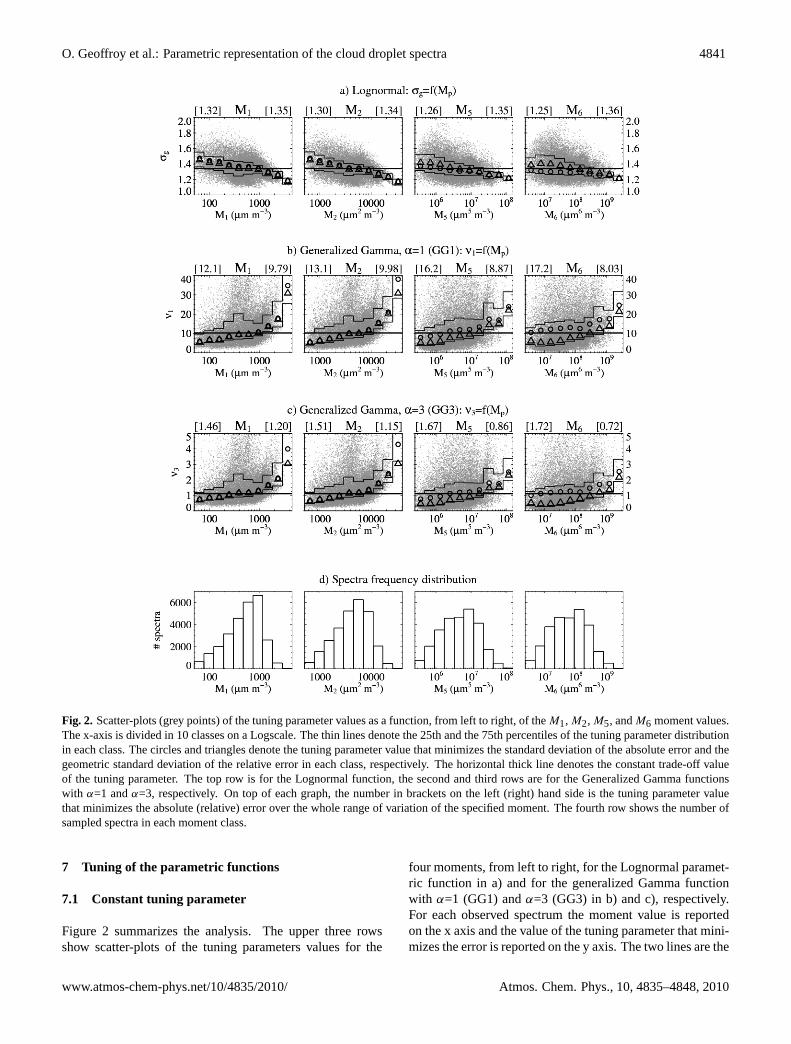
Fig. 2. Scatter-plots (grey points) of the tuning parameter values as a function, from left to right, of theM1, M2, M5, andM6 moment values.

The x-axis is divided in 10 classes on a Logscale. The thin lines denote the 25th and the 75th percentiles of the tuning parameter distribution

in each class. The circles and triangles denote the tuning parameter value that minimizes the standard deviation of the absolute error and the

geometric standard deviation of the relative error in each class, respectively. The horizontal thick line denotes the constant trade-off value of

the tuning parameter. The top row is for the Lognormal function, the second and third rows are for the Generalized Gamma functions withα=1

andα=3, respectively. On top of each graph, the number in brackets on the left (right) hand side is the tuning parameter value that minimizes

the absolute (relative) error over the whole range of variation of the specified moment. The fourth row shows the number of sampled spectra in

each moment class.

20

Fig. 2. Scatter-plots (grey points) of the tuning parameter values as a function, from left to right, of theM1, M2, M5, andM6 moment values.The x-axis is divided in 10 classes on a Logscale. The thin lines denote the 25th and the 75th percentiles of the tuning parameter distributionin each class. The circles and triangles denote the tuning parameter value that minimizes the standard deviation of the absolute error and thegeometric standard deviation of the relative error in each class, respectively. The horizontal thick line denotes the constant trade-off valueof the tuning parameter. The top row is for the Lognormal function, the second and third rows are for the Generalized Gamma functionswith α=1 andα=3, respectively. On top of each graph, the number in brackets on the left (right) hand side is the tuning parameter valuethat minimizes the absolute (relative) error over the whole range of variation of the specified moment. The fourth row shows the number ofsampled spectra in each moment class.

7 Tuning of the parametric functions

7.1 Constant tuning parameter

Figure 2 summarizes the analysis. The upper three rowsshow scatter-plots of the tuning parameters values for the

four moments, from left to right, for the Lognormal paramet-ric function in a) and for the generalized Gamma functionwith α=1 (GG1) andα=3 (GG3) in b) and c), respectively.For each observed spectrum the moment value is reportedon the x axis and the value of the tuning parameter that mini-mizes the error is reported on the y axis. The two lines are the



Fig. 3. Scatter-plots (grey points) of the absolute errors between the observed spectrum moment value and the

one of the parametric function using the trade-off value of the tuning parameterσ∗g=1.34 for the Lognormal

function (top row),ν∗1=10.3 for GG1 (2nd row), andν∗

3=1.11 for GG3 (3rd row), as a function of the moment

values. The X-axis is divided in 10 classes as in Fig. 2. The thin lines denote the 25th and the 75th percentiles

of the absolute error distribution in each class. The circles and the error bars denote the arithmetic mean and

the arithmetic standard deviation of the absolute error values in each class. The absolute errors are normalized

from left to right respectively by 100µm cm−3 for M1, 1000µm2 cm−3 for M2, 107 µm5 cm−3 for M5 and

109 µm6 cm−3 for M6.

21

Fig. 3. Scatter-plots (grey points) of the absolute errors between the observed spectrum moment value and the one of the parametric functionusing the trade-off value of the tuning parameterσ∗

g=1.34 for the Lognormal function (top row),ν∗1=10.3 for GG1 (2nd row), andν∗

3=1.11for GG3 (3rd row), as a function of the moment values. The X-axis is divided in 10 classes as in Fig. 2. The thin lines denote the 25thand the 75th percentiles of the absolute error distribution in each class. The circles and the error bars denote the arithmetic mean and thearithmetic standard deviation of the absolute error values in each class. The absolute errors are normalized from left to right respectively by100 µm cm−3 for M1, 1000 µm2 cm−3 for M2, 107 µm5 cm−3 for M5 and 109 µm6 cm−3 for M6.

25th and the 75th percentile of the corresponding distributionover 10 classes on a Logscale. The circles and triangles arethe tuning parameter values that minimize, in each momentclass, the arithmetic and the geometric standard deviation ofthe absolute and relative errors, respectively. The number ofsamples in each class are reported on the lower row.

For the Lognormal distribution, the top row suggests that aσ g value between 1.3 and 1.4 provides accurate estimations,for the moment values that are the most frequently observed,i.e. 103 µm cm−3 for M1, 5.103 µm2 cm−3 for M2, from 106

to 2.107 µm5 cm−3 for M5 and from 107 to 2.108 µm6 cm−3

for M6. ForM1 andM2, however, this value underestimatesthe optimumσg value at small moment values, hence overes-timates the small moment values, and inversely for the largemoment values. For the higher moments,M5 andM6, the op-timumσ g value does not vary significantly with the value ofthe moment. The sensitivity test to the radius threshold valuethat separates droplets from drops in the bulk scheme reveals

that these two higher moments are more sensitive than thelower ones, although the impact, even with a threshold valueof 27.5 µm, is hardly noticeable. Thisσ g value is close tothe revised value that was recommended in the 9th inter-comparison exercise of the GCSS BLWG (σ g=1.2) for theparameterization of cloud droplet sedimentation (Ackermanet al., 2008).

For the Generalised Gamma distribution, the results aresimilar, with optimum values of the tuning parameterν ofthe order of 10 for GG1 and slightly larger than 1 for GG3,although the trends are reversed compared to the Lognor-mal since increasing values of theν parameters correspondto narrower spectra. A value ofν3 equal to 1 correspondsin the formulation of the autoconversion in Seifert and Be-heng (2006, Eq. 4) to aνc value equal to 0, which is com-monly used.



Fig. 4. Same as Fig. 3 for the relative errors. The circles and the error bars denote the geometric mean and the

geometric standard deviation of the relative error value distribution in each moment class. The relative errors

are not normalized.

22

Fig. 4. Same as Fig. 3 for the relative errors. The circles and the error bars denote the geometric mean and the geometric standard deviationof the relative error value distribution in each moment class. The relative errors are not normalized.

This set of scatter-plots suggests that there is no single pa-rameter value that minimizes both errors for the 4 momentsconcomitantly. The optimum value indeed depends on theapplication and one might select aM1 optimum value forthe prognostic of peak supersaturation in a CCN activationscheme, aM2 specific one for radiative transfer and the sed-imentation flux of particle number concentration, aM5 spe-cific one for the sedimentation flux of particle water content,and aM6 specific one for the retrieval of cloud propertiesfrom a radar reflectivity.

It might be questionable, and less practicable, to use differ-ent values of the tuning parameter for the analytical functionthat describes the droplet distribution in a numerical model,although this is a common practice when using in a numeri-cal model parameterizations of diverse origins, hence relyingon different values of the tuning parameter or even differentparametric functions. For instance the bulk microphysicalschemes tested by the GCSS boundary layer working groupare based on a Lognormal function for parameterization ofdroplet sedimentation (Ackerman et al., 2008), whereas theautoconversion scheme often relies on different hypotheses.Some authors use different distribution hypotheses in the

same process parameterization (see Table 1 in Gilmore andStraka, 2008). For better consistency, we propose a compro-mise that partly satisfies all types of applications. A trade-offvalue of the tuning parameter is derived as:

p∗=

1

8n

∑i,j,k

ni,jpi,j,k, (9)

wheren is the total number of cloud samples,i∈[1:10] standfor the moment class,j∈[1,2,5,6] stands for the moment, andk∈[1,2], corresponds to either the absolute or relative error.ni,j , is the number of samples in classi of the momentMj

andpi,j,k, is the optimum tuning parameter value in the classi of the momentj , for the absolute and relative errors, re-spectively.

This trade-off value of the tuning parameter,σ ∗g=1.34 for

the Lognormal,ν∗

1=10.3 for GG1 andν∗

3=1.11 for GG3, isrepresented in Fig. 2 by a horizontal bar and it is reported inTable 2, with the resulting offset and standard deviations ofthe absolute and relative errors.

Figure 3 shows scatter-plots of the absolute errors in eachmoment class, as in Fig. 2, for the Lognormal (first row), theGG1 (second row) and the GG3 (third row) parametric func-tions. The circles and error bars indicate the arithmetic mean



Fig. 5. Same as Fig. 2 but plotted as a function of the LWC,qc. The thick line represents the proposed

parameterizations for the variable tuning parameter.

23

Fig. 5. Same as Fig. 2 but plotted as a function of the LWC,qc. The thick line represents the proposed parameterizations for the variabletuning parameter.

(offset) and standard deviation of the absolute error values ineach class. Note that for practical reasons, the error valuesare normalized in each graph, as specified in the figure cap-tion. Figure 4 is similar for the relative errors, although errorsare not normalized in this case. These figures confirm that asingle parameter value provides accurate descriptions of thedroplet spectra in the most common range of moment values,but significantly deviates at low moment values for the rela-tive error and high moment values for both errors, althoughsuch samples are less frequently observed.

7.2 Variable tuning parameter

In a second step, we explore the potential of diagnosing thetuning parameter, using the prognostic variables of a bulkparameterization, i.e.N or qc. The tuning parameter showsa noticeable sensitivity toqc, and almost no sensitivity toN .The sensitivity toqc is illustrated in Fig. 5 that is similar toFig. 2, except that the x-axis now represents the LWC.

The optimum parameter values, in eachqc class(10 classes) of each moment (4 moments) and for boththe absolute (circles) and relative (triangles) errors, are



Fig. 6. Same as Fig. 3 using the proposed parameterization for the variable tuning parameter.

24


combined and the function ofqc that best fits the 80 valuesis derived for the Lognormal, the GG1 and the GG3 succes-sively, leading to the following parameterizations:

σpg = −0.056· ln(qc)+1.24, (10)

νp

1 = 14.5·qc +6.7, (11)

νp

3 = 1.58·qc +0.72, (12)

whereqc is expressed in g m−3. They are represented in eachgraph of Fig. 5 by a thick line.

Figures 6 and 7, similar to Figs. 3 and 4 show the improve-ment on the absolute and relative errors, respectively, in eachmoment class. The offsets and standard deviations of the ab-solute and relative errors over the whole range of momentvalues are summarized in Table 3.

The comparison with Table 2, attests that both the absoluteand relative errors have been reduced in term of offset andstandard deviation, although the main improvement is for theabsolute error at large values of the moments (Figs. 3 and 6),and for the relative error at both small and large values of themoments (Figs. 4 and 7).

8 Summary and conclusions

Droplet spectra measured in stratocumulus and shallow cu-mulus clouds have been examined to fit three parametricfunctions, i.e. the Lognormal, and the Generalized Gammafunctions withα=1 andα=3, successively, that are frequentlyused in bulk parameterizations of the microphysics to repre-sent droplet size distributions.

These functions have three independent parameters. Twoare constrained by the values of the droplet number concen-tration and liquid water content. An optimum value of thethird parameter,σ g for the Lognormal,ν1 for the GG1 andν3for the GG3, has been derived for each measured spectrum,that minimizes the difference between the observed spectrumand the parametric function. The difference has been mea-sured using integral properties of the droplet spectra, namely4 moments of the size distribution,M1 that is used in CCNactivation schemes,M2 in radiative transfer calculations anddroplet sedimentation parameterization,M5 for parameteri-zation of droplet sedimentation, andM6 for radar reflectivitycalculations.




25


Table 3. Same as Table 2 when using the variable tuning parameter parameterizations,σpg for the Lognormal,νp

1 for the GG1 andνp3 for the

GG3.

M1 M2 M5 M6

Lognormal, µabs±σabsσ

pg 4.3±28.9 23±227 0.2±18.2 1.2±54.2

(µm cm−3) (µm2 cm−3) (105 µm5 cm−3) (106µm6 cm−3)

µrel×

/ σ rel

1.007×/ 1.052 1.003×/ 1.050 0.978×/ 1.292 0.918×/ 1.651

Generalized Gamma, µabs±σabsα=1, νp

1 −2.3±29.0 −17±226 0.3±18.1 −1.4±53.5(µm cm−3) (µm2 cm−3) (105µm5 cm−3) (106µm6 cm−3)

µrel×

/ σ rel

0.997×/ 1.053 0.996×/ 1.050 0.973×/ 1.300 0.893×/ 1.672

Generalized Gamma, µabs±σabsα=3, νp

3 −8.6±29.9 −37±226 −1.7±18.0 −8.9±52.7(µm cm−3) (µm2 cm−3) (105µm5 cm−3) (106µm6 cm−3)

µrel×

/ σ rel

0.984×/ 1.052 0.990×/ 1.050 0.943×/ 1.303 0.826×/ 1.682



The range of variation of each moment has been dividedin 10 classes on a Logscale and the arithmetic and geometricmeans of the optimum parameter values have been calculatedin each class. The absolute and relative errors have similarlybeen quantified in each class, and over the whole range ofvariation of each moment. As expected, the optimum param-eter values however are slightly different depending on whichintegral property is used for the minimization. A trade-offparameter value has then been proposed, that minimizes boththe absolute and the relative errors on the 4 moments of thedistributions.

In a second step, parameterizations are proposed where theoptimum parameter value depends on the LWC, and the ab-solute and relative errors have been quantified for each mo-ment separately. Such a varying tuning parameter slightlyimproves both the absolute and relative errors for the mo-ment values that are the most frequently observed, and it sig-nificantly improves the error at the lowest and largest valuesof the moments.

The potential of using the third parameter as a prognos-tic variable in a bulk scheme has been explored, but becauseof the large variability of spectral shapes and the diversityof physical processes that are responsible for this variabil-ity, condensational growth, mixing and evaporation, dropletscavenging, and collection, we have not been able to isolateone process that could be considered as the most determinant.Further analysis or numerical simulations with bin micro-physical schemes might help at solving the issue. However,considering the limitations inherent to the bulk approach, onemight also conclude that the accuracy of the parameteriza-tions proposed here is sufficient for most of the topics thatcan be addressed with a bulk scheme.

Acknowledgements.This study has been partially supportedby the Netherlands Organization for Scientific Research underGrant 854.00.032 and by the European Commission 6th Frame-work program project EUCAARI (European Integrated project onAerosol Cloud Climate and Air Quality interactions) No 036833-2.RICO data other than Fast-FSSP measurements were provided byNCAR/EOL under sponsorship of the National Science Foundation(http://data.eol.ucar.edu/). The authors acknowledge the contribu-tion of the Meteo-France TRAMM team for ACE2 data processing.The authors also thank the two anonymous reviewers and PierSiebesma for their comments that helped to improve the manuscript.

Edited by: V.-M. Kerminen

References

Ackerman, A. S., van Zanten, M. C., Stevens, B., Savic-Jovcic,V., Bretherton, C. S., Chlond, A., Gloaz, J.-G., Jiang, H.,Khairoutdinov, M., Krueger, S. K., Lewellen, D. C., Lock, A.,Moeng, C.-H., Nakamura, K., Petters, M. D., Snider, J. R.,Weinbrecht, S., and Zulauf, M.: Large-eddy simulations of adrizzling, stratocumulus-topped marine boundary layer, Mon.Weather Rev., 137, 1083–1110, 2008.

Atlas, D.: The estimation of cloud parameters by radar, J. Meteorol.,11, 309–317, 1954.

Berry, E. X. and Reinhardt, R. L.: An analysis of cloud drop growthby collection Part II. Single initial distributions, J. Atmos. Sci.,31, 1825–1831, 1974.

Brenguier, J.-L., Bourrianne, T., de Araujo Coelho, A., Isbert, R.J., Peytavi, R., Trevarin, D., and Weschler, P.: Improvements ofdroplet distribution size measurements with the fast-FSSP (for-ward scattering spectrometer probe), J. Atmos. Ocean. Tech., 15,1077–1090, 1998.

Brenguier, J.-L., Pawlowska, H., Schuller, L., Preusker, R., Fis-cher, J., and Fouquart, Y.: Radiative properties of boundary layerclouds: droplet effective radius versus number concentration, J.Atmos. Sci., 57, 803–821, 2000.

Brenguier, J.-L., Pawlowska, H., and Schuller, L. J.: Cloud micro-physical and radiative properties for parameterization and satel-lite monitoring of the indirect effect of aerosol on climate, J. Geo-phys. Res., 108, 8632, doi:10.1029/2002JD002682, 2003.

Burnet, F., and Brenguier, J.-L.: Validation of droplet spectra andliquid water content measurements, Phys. Chem. Earth (B), 24,249–254, 1999.

Burnet, F., and Brenguier, J.-L.: Comparison between standard andmodified forward scattering spectrometer probes during the smallcumulus microphysics study, J. Atmos. Oceanic Tech., 19, 1516–1939, 2002.

Burnet, F., and Brenguier, J.-L.: Observational study of theentrainment-mixing process in warm convective clouds, J. At-mos. Sci., 64, 1995–2011, 2007.

Clark, T. L.: Use of log-normal distributions for numerical calcula-tion of condensation and collection, J. Atmos. Sci., 33, 810–821,1976.

Cohard, J.-M. and Pinty, J.-P.: A comprehensive warm microphysi-cal bulk scheme, part I: Description and selective tests, Q. J. Roy.Meteor. Soc., 126, 1815–1842, 2000.

Feingold, G. and Levin, Z.: The lognormal fit to raindrop spectrafrom frontal convective clouds in Israel, J. Clim. Appl. Meteorol.,25, 1346–1363, 1986.

Gilmore, M. S. and Straka, J. M.: The Berry and Reinhardt auto-conversion : A digest. J. Appl. Meteorol., 47, 375–396, 2008.

Hansen, J. E. and Travis, L. D.: Light scattering in planetary atmo-spheres, Space Sci. Rev., 16, 527–610, 1974.

Kessler, E.: On the Distribution and Continuity of Water Substancein Atmospheric Circulations, Meteor. Monogr., 32, Amer. Me-teor. Soc., 84 pp., 1969.

Khairoutdinov, M. and Kogan, Y.: A new cloud physics parameteri-zation in a large-eddy simulation model of marine stratocumulus,Mon. Weather Rev., 128, 229–243, 2000.

Kogan, Y.: The simulation of a convective cloud in a 3-D modelwith explicit microphysics. Part I: Model description and sensi-tivity experiments, J. Atmos. Sci., 48, 1160–1189, 1991.

Martin, G. M., Johnson, D. W., and Spice, A.: The measurementand parameterization of effective radius of droplets in warm stra-tocumulus clouds, J. Atmos. Sci., 51, 1823–1842, 1994.

Lawson, R. P., O’Connor, D., Zmarzly, P., Weaver, K., Baker, B.,Mo, Q. and Jonsson, H.: The 2D-S (Stereo) probe: design andpreliminary tests of a new airborne, highspeed, high-resolutionparticle imaging probe, J. Atmos. Oceanic Tech., 23, 1462–1477,2006.

Liu, Y., You, Y., Yang, W., and Liu, F.: On the size distribution of


http://data.eol.ucar.edu/


cloud droplets, Atmos. Res., 35, 201–216, 1995.Liu, Y. and Hallett, J.: On size distributions of cloud droplets grow-

ing by condensation: A new conceptual model, J. Atmos. Sci.,55, 527–536, 1998.

Liu, Y. and Daum, P. H.: Spectral dispersion of cloud droplet sizedistributions and the parameterization of cloud droplet effectiveradius, Geophys. Res. Lett., 27, 1903–1906, 2000.

Liu, Y. and Daum, P. H.: Parameterization of the autoconversionprocess. Part I: Analytical formulation of the Kessler-type pa-rameterizations, J. Atmos. Sci., 61, 1539–1548, 2004.

Manton, M. J. and Cotton, W. R.: Formulation of approximate equa-tions for modeling moist deep convection on the mesoscale, At-mos. Sci., 266, Dept. of Atmos. Sci., Colorado State University,1977.

Milbrandt, J. A. and Yau, M. K.: A multimoment bulk microphysicsparameterization. Part II: A proposed three-moment closure andscheme description, J. Atmos. Sci., 62, 3065–3081, 2005.

Pawlowska, H., Brenguier, J.-L., and Salut, G.: Optimal non-linearestimation for cloud particle measurements, J. Atmos. Ocean.Tech., 14, 88–104, 1997.

Pawlowska, H. and Brenguier, J.-L.: An observational study ofdrizzle formation in stratocumulus clouds for general circulationmodel (GCM) parameterizations, J. Geophys. Res., 108(D15),8630, doi:10.1029/2002JD002679, 2003.

Rogers, R. R. and Yau, M. K.: A Short Course in CloudPhysics, Third edition, International Series in Natural Philoso-phy, Pergammon Press, 293 pp., 1989.

Rauber, R. M., Stevens, B., Ochs, H. T., Knight, C., Albrecht, B.A., Blyth, A. M., Fairall, C. W., Jensen, J. B., Lasher-Trapp, S.G., Mayol-Bracero, O. L., Vali, G., Anderson, J. R., Baker, B. A.,Bandy, A. R., Burnet, F., Brenguier, J.-L., Brewer, W. A., Brown,P. R. A., Chuang, P., Cotton, W. R., Di Girolamo, L., Geerts,B., Gerber, H., Goke, S., Gomes, L., Heikes, B. G., Hudson,J. G., Kollias, P., Lawson, R. P., Krueger, S. K., Lenschow, D.H., Nuijens, L., O’Sullivan, D. W., Rilling, R. A., Rogers, D.C., Siebesma, A. P., Snodgrass, E., Stith, J. L., Thornton, D.C., Tucker, S., Twohy, C. H., and Zuidema, P.: Rain in shallowcumulus over the ocean: The RICO campaign, B. Am. Meteorol.Soc., 88, 1912–1928, 2007.

Seifert, A. and Beheng, K. D.: A double-moment parameterizationfor simulating autoconversion, accretion and self-collection, At-mos. Res, 59–60, 265–281, 2001.

Seifert, A. and Beheng, K. D.: A two-moment cloud microphysicsparameterization for mixed-phase clouds. Part 1: Model descrip-tion, Meteorol. Atmos. Phys., 92, 45–66, 2006.

Tripoli, G. J. and Cotton, W. R.: A numerical investigation of sev-eral factors contributing to the observed variable intensity of deepconvection over South Florida, J. Atmos. Sci., 19, 1037–1063,1980.

Twomey, S.: The nuclei of natural cloud formation. Part II: The su-persaturation in natural clouds and the variation of cloud dropletconcentration, Geofys. Pura. Appl., 43, 243–249, 1959.

Warner, J.: The microstructure of cumulus clouds. Part I. Generalfeatures of the droplet spectrum, J. Atmos. Sci., 26, 1049–1059,1969a.

Warner, J.: The microstructure of cumulus clouds. Part II. The ef-fect on droplet size distribution of cloud nucleus spectrum andupdraft velocity, J. Atmos. Sci., 26, 1272–1282, 1969b.

Warner, J.: The microstructure of cumulus clouds. Part III. The na-ture of the updraft, J. Atmos. Sci., 27, 682–688, 1970.

Warner, J.: The microstructure of cumulus clouds. Part IV. The ef-fect on the droplet spectrum of mixing between cloud and envi-ronment, J. Atmos. Sci., 30, 256–261, 1973a.

Warner, J.: The microstructure of cumulus clouds. Part V. Changesin droplet size distribution with cloud age, J. Atmos. Sci., 30,1724–1726, 1973b.

Williams, R. and Wojtowicz, P. J.: A Simple Model for DropletSize Distribution in Atmospheric Clouds, J. Appl. Meteorol., 21,1042–1044, 1982.

Ziegler, C. L.: Retrieval of thermal and microphysical variables inobserved convective storms. Part I: Model development and pre-liminary testing, J. Atmos. Sci., 42, 1487–1509, 1985.


Documents

Parametric representation of the cloud droplet spectra … · 1Royal Netherlands Meteorological Institute (KNMI), De Bilt, The Netherlands ... (CDSD), the parameterized microphysical