Parametric Mixture Models for Estimating the Proportion of ...users.iems.northwestern.edu/~ajit/papers/45) FDR Paper.pdf · model assumes that the test statistics from the true null

Parametric Mixture Models for Estimating the Proportion of True Null Hypotheses andAdaptive Control of FDRAuthor(s): Ajit C. Tamhane and Jiaxiao ShiSource: Lecture Notes-Monograph Series, Vol. 57, Optimality: The Third Erich L. LehmannSymposium (2009), pp. 304-325Published by: Institute of Mathematical StatisticsStable URL: http://www.jstor.org/stable/30250047Accessed: 22/10/2010 10:25

Your use of the JSTOR archive indicates your acceptance of JSTOR's Terms and Conditions of Use, available athttp://www.jstor.org/page/info/about/policies/terms.jsp. JSTOR's Terms and Conditions of Use provides, in part, that unlessyou have obtained prior permission, you may not download an entire issue of a journal or multiple copies of articles, and youmay use content in the JSTOR archive only for your personal, non-commercial use.

Please contact the publisher regarding any further use of this work. Publisher contact information may be obtained athttp://www.jstor.org/action/showPublisher?publisherCode=ims.

Each copy of any part of a JSTOR transmission must contain the same copyright notice that appears on the screen or printedpage of such transmission.

JSTOR is a not-for-profit service that helps scholars, researchers, and students discover, use, and build upon a wide range ofcontent in a trusted digital archive. We use information technology and tools to increase productivity and facilitate new formsof scholarship. For more information about JSTOR, please contact [email protected].

Institute of Mathematical Statistics is collaborating with JSTOR to digitize, preserve and extend access toLecture Notes-Monograph Series.

http://www.jstor.org

http://www.jstor.org/action/showPublisher?publisherCode=ims

http://www.jstor.org/stable/30250047?origin=JSTOR-pdf

http://www.jstor.org/page/info/about/policies/terms.jsp

http://www.jstor.org/action/showPublisher?publisherCode=ims

IMS Lecture Notes-Monograph Series Optimality: The Third Erich L. Lehmann Symposium Vol. 57 (2009) 304-325 @ Institute of Mathematical Statistics, 2009 DOI: 10. 1214/09-LNMS5718

Parametric Mixture Models for

Estimating the Proportion of True Null

Hypotheses and Adaptive Control of FDR

Ajit C. Tamhanel and Jiaxiao Shi2

Northwestern University

Abstract: Estimation of the proportion or the number of true null hypotheses is an important problem in multiple testing, especially when the number of

hypotheses is large. Wu, Guan and Zhao [Biometrics 62 (2006) 735-744] found that nonparametric approaches are too conservative. We study two parametric mixture models (normal and beta) for the distributions of the test statistics or their p-values to address this problem. The components of the mixture are the null and alternative distributions with mixing proportions 7ro and 1 - r7o, respectively, where 7ro is the unknown proportion to be estimated. The normal model assumes that the test statistics from the true null hypotheses are i.i.d.

N(0, 1) while those from the alternative hypotheses are i.i.d. N(6, 1) with 6 5 0. The beta model assumes that the p-values from the null hypotheses are i.i.d. U[0, 1] and those from the alternative hypotheses are i.i.d. Beta(a, b) with a < 1 < b. All parameters are assumed to be unknown. Three methods of estimation of 7ro are developed for each model. The methods are compared via simulation with each other and with Storey's [J. Roy. Statist. Soc. Ser. B 64 (2002) 297-304] nonparametric method in terms of the bias and mean

square error of the estimators of 7ro and the achieved FDR. Robustness of the estimators to the model violations is also studied by generating data from other models. For the normal model, the parametric methods perform better

compared to Storey's method with the EM method (Dempster, Laird and Rubin [Roy. Statist. Soc. Ser. B 39 (1977) 1-38]) performing best overall when the assumed model holds; however, it is not very robust to significant model violations. For the beta model, the parametric methods do not perform as well because of the difficulties of estimation of parameters, and Storey's nonparametric method turns out to be the winner in many cases. Therefore the beta model is not recommended for use in practice. An example is given to illustrate the methods.

Contents

1 Introduction ...............305 2 Normal Model 307

2.1 Hsueh, Chen, and Kodell (HCK) Method 307 2.2 Test Statistics (TS) Method 308 2.3 EM Method 309

3 Beta Model 310 3.1 Hsueh, Chen, and Kodell (HCK) Method 310 3.2 Test Statistics (TS) Method 311 3.3 EM Method 312

1Department of IEMS, Northwestern University, Evanston, IL 60208 2Department of Statistics, Northwestern University, Evanston, IL 60208 AMS 2000 subject classifications: Primary 62F10; secondary 62F12. Keywords and phrases: Beta model, bias-correction, EM method, mixture model, false discov-

ery rate (FDR), least squares method, maximum likelihood method, normal model, p-values.

304

Parametric Mixture Models 305

4 Adaptive Control of FDR 313 5 Simulation Results 314

5.1 Simulation Results for Normal Model 314 5.2 Robustness Results for Data Generated by Beta Model 317 5.3 Simulation Results for Beta Model 318

6 Example 320 7 Concluding Remarks 322 Appendix 322 Acknowledgments 324 References 324

1. Introduction

Suppose that m null hypotheses, Ho01,..., Hom, are to be tested against alternatives, H1,... , Him. Let X1,... , Xm be the test statistics and pl, ..., Pm their p-values. Throughout we assume that the Xi's and hence the pi's are mutually independent. Suppose that some unknown number mo of the hypotheses are true and m l= m-mo are false. We wish to estimate mo or equivalently the proportion 7ro = mo/m of the true hypotheses based on the Xi's or equivalently the pi's. The estimate miio is useful for devising more powerful adaptive multiple comparison procedures (MCPs) to control an appropriate type I error rate, e.g., the familywise error rate (FWE) (Hochberg and Tamhane [11]) in the Bonferroni procedure or the false discovery rate (FDR) in the Benjamini and Hochberg [1] procedure. These procedures normally use the total number m as a conservative upper bound on the number of true hypotheses. Adaptive procedures based on mio are especially useful in large-scale multiplicity testing problems arising in microarray data involving m of the order of several thousands.

A number of methods have been proposed for estimating mo starting with Schweder and Spjetvoll [18]; see, e.g., Hochberg and Benjamini [10], Benjamini and Hochberg [2], Turkheimer, Smith and Schmidt [23], Storey [21], Storey et al.

[22], Jiang and Doerge [15] and Langaas et al. [17]. Many of these methods reject the p-values that differ significantly from the null U[0, 1] distribution as non-null and exclude them from the estimation process. Different formal or graphical tests are used for this purpose. For example, consider Storey's [21] method with a fixed A-level test for a sufficiently large A (e.g., A = 0.5) to reject any p-value < A as non-null. (It should be noted that in fact A is not fixed but is a tuning parameter whose value is determined from the data to minimize the mean square error of the estimate of 7ro using bootstrap.) Let Nr(A) = (pi 5 A) denote the number of rejected hypotheses and Na(A) = O(Pi > A) the number of accepted hypotheses at level A e (0, 1). If type II errors are ignored for a sufficiently large A then

(1.1) E[Na(A)] r mo(1 - A).

Storey's (ST) estimator is given by

. N'(>) Na(A) (1.2) 0o(1A) =

or mo0(A) = - m(1 - A) 1 - A

Schweder and Spjotvoll's [18] method visually fits a straight line through the origin to the plot of Na(p(i)) = m - i vs. 1 - p(i) (1 < i < m) for large values of the P(i). The slope of the fitted line is taken as an estimate of mo according to Equation (1.1). Because these estimators attribute all nonsignificant p-values to the true null hypotheses (type II errors are ignored) and do not explicitly model

306 Tamhane and Shi

the non-null p-values, they tend to be positively biased which results in conservative adaptive control of any type I error rate.

To get a handle on type II errors, so that both the null and non-null p-values can be utilized to estimate or0, the mixture model approach has been proposed by several authors. The mixture model differs from the setup given in the first paragraph in that the number of true hypotheses is a random variable (r.v.) and mo is its expected value. Specifically, let Zi be a Bernoulli r.v. which equals 1 with probability rr0 if

Hoi is true and 0 with probability ri = 1 - io if Hoi is false. Assume that the Zi (1 < i < m) are i.i.d. Then the number of true hypotheses, Mo =

Z~= Zi, is a binomial r.v. with parameters m and 7ro, and E(Mo) = mo = m-ro.

A parametric mixture model was considered by Hsueh, Chen, and Kodell [12] (HCK). They assumed the following simple hypothesis testing setup. Suppose that all m hypotheses pertain to the means of the normal distributions with Hoi : i = 0 versus Hli : pi > 0. (HCK considered a two-sided alternative, but that is not

germane to their method.) Conditional on Zi, the test statistic Xi ~ N(6i, 1), where 6i is the standardized lpi with 6i = 0 if Zi = 1 and 6i = 6 > 0 if Zi = 0 where HCK assumed that S is known. We refer to this model as the normal model, which was also used by Black [3] to study the bias of Storey's [21] estimator. An

expression for the expected number of Xi's that are greater than any specified threshold can be derived using this setup. By plotting the corresponding observed number of Xi's against the threshold, mo could be estimated as the slope of the

straight line through the origin using least squares (LS) regression. The normal model is the topic of Section 2. We first extend the HCK estimation

method to the unknown 6 case, which is a nonlinear least squares (NLS) regression problem. Next we note that the HCK method makes use of only the number of Xi's that are greater than a specified threshold; it does not make use of the magnitudes of the Xi's. Therefore we propose two alternative methods of estimation which uti- lize the magnitudes of the Xi's in an attempt to obtain a better estimate of 6 and

thereby a better estimate of mo. The first of these alternative methods is similar to the LS method of HCK, but uses the sample mean (instead of the number) of the Xi's that are greater than a specified threshold. We refer to it as the test statistics (TS) method. The second method is the EM method of Dempster, Laird and Rubin [4] which finds the maximum likelihood estimators (MLEs) of the mixture distribution of the Xi's.

This normal mixture model approach in conjunction with the EM algorithm was

proposed by Guan, Wu and Zhao [8] and most recently by Iyer and Sarkar [14]. So, although the use of the EM algorithm for estimation in the context of the present problem is not new, we perform a comprehensive comparison of it with the other two new methods, and find that it performs best when the assumed model is correct, but is not robust to model violations.

In the second approach discussed in Section 3, the non-null p-values are modeled

by a beta distribution with unknown parameters a and b (denoted by Beta(a, b)). We refer to this model as the beta model. Here we restrict to estimation methods based on p-values since the Xi's can have different null distributions. All three estimators (HCK, TS and EM) are also derived for the beta model.

We stress that both the normal and beta models are simply '"working" models intended to get a handle on type II errors. We do not pretend that these models are strictly true. Therefore robustness of the estimators to the model assumptions is an important issue. In the simulation comparisons for the normal model, robustness of the fixed 6 assumption is tested by generating different (5's for the false hypotheses from a normal distribution. Robustness of the normal model assumption is tested by


generating pi's for the false hypotheses using the beta model and transforming them to the Xi's using the inverse normal transformation. Similarly, the robustness of the beta model is tested by generating Xi's using the normal model and transforming them to pi's.

Adaptive control of FDR using different estimators of mo is the topic of Sec- tion 4. The ST, HCK, TS and EM estimators are compared in a large simulation

study in Section 5. The performance measures used in the simulation study are the biases and mean square errors of the estimators of ro and FDR. An example illus-

trating application of the proposed methods is given in Section 6. Conclusions are summarized in Section 7. Proofs of some technical results are given in the Appendix.

2. Normal Model

The normal mixture model can be expressed as

(2.1) f(xi) = 7roA(xi) + airl(xi - 6),

where f(xi) is the p.d.f. of Xi and 0(.) is the p.d.f. of the standard normal distribution. Although 6 will need to be estimated, we are not too concerned about its estimation accuracy since, after all, it is a parameter of a working model.

2.1. Hsueh, Chen, and Kodell (HCK) Method

Let

(2.2) 0(6, A) = PHlI{Pi > A} = PHI {Xi < zA} = " (zA - 6)

denote the type II error probability of a test performed at level A where D(.) is the standard normal c.d.f. and zA - (-1(1- A). Then E[Nr(A)] = moA + (m-mo)[1- 3(6, A)], and hence

(2.3) E[Nr(A)] - mb (-zA + 6) = mo[A - 4P (-zA + 6)]. For A = p(i), i = 1, 2,..., m, the term inside the square brackets in the R.H.S. of the above equation is

(2.4) i = p(i) - 4 (-zp(, + 6) and the L.H.S. can be estimated by

(2.5) y, = i - (-zP(,) + 6).

If 6 is assumed to be known then we can calculate (xi, yi), i = 1, 2,..., m, and using (2.3) fit an LS straight line through the origin by minimizing 1 _(y, - moxi)2 with respect to (w.r.t.) mo. The LS estimator of mo is given by

SEi)=1 xiyi (2.6) mio =-

m AA ml2 "

We first extend the HCK estimator to the unknown 6 case by incorporating estimation of 6 as part of the NLS problem of minimizing Zml=(yi - moxi)2 w.r.t. mo and 6. The iterative algorithm for this purpose is given below. The initial values

308 Tamhane and Shi

for this algorithm as well as the algorithms for the TS and EM estimators were determined by solving the following two moment equations for mo and 6:

m m

(2.7) Xi = (m - mo)6 and X2 = m0 + (m - mo)(62 + i=1 i=1

HCK Algorithm Step 0: Compute initial estimates mio and 6 by solving (2.7). Let ro =

-io/m. Step 1: Set 6 = 6 and compute (xi, y), i = 1, 2,..., m, using (2.4) and (2.5). Step 2: Compute mio using (2.6) and ro = iio/m. Step 3: Find 6 to minimize Ei=l(yi

- moxi)2

Step 4: Return to Step 1 until convergence.

Remark. One could use weighted least squares to take into account the het- eroscedasticity of the yi's. We tried this, but the resulting NLS problem was com- putationally much more intensive without a collateral gain in the efficiency of the estimators.

2.2. Test Statistics (TS) Method

As noted in Section 1, we hope to improve upon the HCK estimator by utilizing the information in the magnitudes of the Xi's. Toward this end we first propose an estimator analogous to the HCK estimator except that it uses the sample mean

(rather than the number) of the Xi's that are significant at a specified level A. Define

Sa(A) = {i: pi > A}{= i :Xi < zA} and S,(A) = {i: pi ( i:Xi > zA.

Then Na(A) = ISa(A)I and Nr(A) = ISr(A)I. Finally define

1 1 Xa(A)

= 1 Xi and Xr,(A)N(A) Xi.

sNa(A)ESa(A) iESr(A)

To derive the expected values of these sample means the following lemma is useful.

Lemma 1. Define

coa(A) = EHoi (Xi4Xi < zA) , Cr(A) =

EHo, (Xi|Xi zA),

Cla(6,1A) = EHli (XilXi < zA) ,c1l(6, A) = EH1i (XilXi X

zA) .

and

Then

and Coa(A (zA)cor(A)- (zA)

1( - - A

Cla(6,A) -=6 - (z - 6)

-)Clr(6 a

A)( + -Z) C(zA - 6)O) ( - ZA)

Proof. The proof follows from the following expressions for the conditional expec- tations of X ~ N(1i, 1):

E(XIX x) = -( and E(XIX > x) = ( +

-x) E(IX< )- ,D

(x - CA)X


The desired expected values of Xa(A) and Xr(A) are then given by the following lemma.

Lemma 2. Let

pro(1 - A) (2.8) g(iro, 6, A) = P {Zi = Xi < z} r (1 - A) -xo (1 -

A) + rrl 4) (zA -

6)

and

(2.9) h(7ro, 6, A) = P (Zi = 1Xi A> zA} = roA

7roA + rI (-zA + 6)

Then

(2.10) E[X,(A)] = g(iro, 6, A)co0a(A) + [1 - g(lro, 6, A)]clia(6, A)

and

(2.11) E[Xr (A)] = h(ro, 6, A)cor(A) + [1 - h(7ro, 6, A)]Cr(6,lA),

where coa(A)), cor(A), cla(6, A) and cl,(6, A) are as given in Lemma 1.

Proof. Given in the Appendix. El

To develop an estimation method analogous to the HCK method note that from (2.3) and (2.11) we get

(2.12) E[Nr(A)]E[Xr(A)] - mJA (-ZA + 6) clr(6, A) -= mo [Acor(A) - ( (-zA + 6) clr(6, A)].

For A = p(i), i = 1, 2,..., m, the term inside the square brackets in the R.H.S. of the above equation is

(2.13) xi =

p(i)Cor(P(i)) - 4 (-zp -

+ 6) Clr(6,P(i))

and the L.H.S. can be estimated by

Yi = iXr(P(i)) - m(1 (-zp(i) + 6) clr(6, p(i)) m

(2.14) = E X(j) - m(J (-zp(-)

+ 6) Clr(6, p(i)). j=m-i+l

Then from (2.12) we see that a regression line of yi versus xi can be fitted through the origin with slope mo by minimizing ~- =(yi - moxi)2 w.r.t. mo and 6. The algorithm to solve this NLS regression problem is exactly analogous to the HCK algorithm.

2.3. EM Method

Whereas the HCK and TS methods compute the LS estimators of or0 and 6 (for two different regression models), the EM method computes their MLEs. For these MLEs to exist, it is necessary that r0o be bounded away from 0 and 1. The steps in the EM algorithm are as follows.

310 Tamhane and Shi

EM Algorithm Step 0: Compute initial estimates miio and 6 by solving (2.7). Let i~o =

-?io/m. Step 1 (E-step): Calculate the posterior probabilities:

Roq(Xi) 7roo(Xi) + 910(Xi - )

and ji(Xi) = 1 - 7o(Xi), i = 1, 2,..., m. Step 2 (M-step): Calculate new estimates:

= 1 o(X) ( -iz1 l(Xi)Xi ro =and 6 = m m E , 7i(Xi)


3. Beta Model

In many applications the normal model may be inappropriate because the test statistics may not be normally distributed or different types of test statistics (e.g., normal, t, chi-square, Wilcoxon, log-rank) may be used to test different hypotheses or only the p-values of the test statistics may be available. In these cases we use the p-values to estimate r0.

We propose to model the non-null p-values by a Beta(a, b) distribution given by

g(pla, b) = F(a +

b)a-1(1 p)b1 r1(a) (b) with unknown parameters a and b with a < 1 and b > 1. This restriction is imposed in order to ensure that g(pla, b) is decreasing in p. It is well-known that the non-null distribution of the p-values must be right-skewed and generally decreasing in shape (see Hung, O'Neill, Bauer and Kohne [13]). Langaas et al. [17] imposed the same restriction in their nonparametric estimate of the non-null distribution of p-values.

Of course, the null distribution of a p-value is Beta(l, 1), i.e., the U[0, 1] distribution. As in the case of the normal model, the beta model can be represented as a mixture model for the distribution of the pi:

(3.1) f(pi) = 7ro x 1 + rlg(pipa, b).

The parameters a and b must be estimated along with 7ro. This problem is analogous to that encountered for the normal model with the difference that in addition to

r0o, we have to estimate two parameters, a and b, instead of a single parameter 6. We first extend the HCK method for the normal model discussed in Section 2.1 to this beta model.

3.1. Hsueh, Chen, and Kodell (HCK) Method

Denote the type II error probability of a test performed at level A by

(3.2) (a, b, A) = PHPi > r(ab) pa-l(1 p)b-ldp = 1 - IA(a, b),

where IA (a, b) is the incomplete beta function. Put

(3.3) xi = P(i) - Ip(,) (a, b) and yi = i - mlP(,) (a, b).


Then the HCK method amounts to solving the NLS problem of minimizing

A 1(Yi - mOXi)2 w.r.t. mo and (a, b) (subject to a < 1 < b). Gauss-Newton

method (Gill et al. [7]) was used to perform minimization w.r.t. (a, b). The initial

starting values for this algorithm as well as the algorithms for the TS and EM estimators described below were determined by solving the following three moment equations for mo and (a, b):

m 1 a pi = -mo + mi,

2 a+b i=-1

m 1 a(a + 1) (3.4) m 2= mo+ mi,

i=1

3 (a+b)(a + b + 1) m 3_o1 a(a + 1)(a + 2)

i= 4 (a + b)(a + b + 1)(a + b + 2) i= 1

3.2. Test Statistics (TS) Method

Here the TS estimator is based on the average of the "accepted" or "rejected" p-values defined as

1 1

Pa( Na()A)

= I

E

piandpr(A)- 1r(EA) Pi" Na(A s(Nr() s(A)

Analogous to Lemma 1, we have the following lemma.

Lemma 3. Define

do (A) = EHo (Pi Ip > A) do0r(A) = EHoi (pilpi < A),

dia(a, b, A) = EH1, (pi lpi > A), dir(a, b, A) = EH1, (PAi

< A).

and

Then we have

and

A+1 A doa(A) 2 ,dor(A) 2

7

1 - IA(a + 1, b) a IA(a + 1, b) a 1 - I(a, b) a + b' I (a, b) a + b

Proof. Straightforward. O

The next lemma gives E[,a(A)]

and E[pr(A)]; its proof is exactly analogous to that of Lemma 2.

Lemma 4. Let

aio(1 - A) g(7ro, a, b, A) = P {Zi = 1lpi > Al} = 7o(1 - A)

7ro(1 - ) + 71i [1 - IIA(a, b)]

h(7ro, a, b, A) = P {Zi = 1 lpi < A} 7roA 7rOAA + 7rIA (a, b)

and

312 Tamhane and Shi

Then

(3.5) Epa(A)] = g(rro, a, b, A)doa(A) + [1 - g(7ro, a, b, A)]dia (a, b, A)

and

(3.6) E[r(A)] = h(rro, a, b, A)dor(A) + [1 - h(7ro, a, b, A)]dlr (a, b, A),

where do,(A), dor(A), dia(a, b, A) and dir(a, b, A) are as given in Lemma 3.

The equations for the TS estimator are derived as follows. Analogous to (2.12), we obtain

E[Nr(A)]E[pr(A)] - mIA(a, b)dir(a, b, A) = mo[Ador(A) - IA(a, b)dir (a, b, A)].

For A = p(i), i = 1, 2,..., m, the term in the square brackets in the R.H.S. of the above equation equals

2

P(i) a (a ,b) Xi 2 a+b Ip(,) (a + 1, b)

and the L.H.S. can be estimated by i

Yi EP(j)-a+ Ip(a+1,b). j=a1

The TS algorithm for the normal model can be modified to minimize EAi=l(Yi -

moxi)2 by replacing the minimization with respect to 6 by minimization with respect to (a, b).

3.3. EM Method

The steps in the EM algorithm, which gives the MLEs of 70 and (a, b), are as follows. As in the case of the normal model, for these MLEs to exist, it is necessary that

0ro be bounded away from 0 and 1.

Step 0: Initialize o0 and (a, b) by solving (3.5). Let r0o

= io/m. Step 1 (E-Step): Calculate the posterior probabilities:

7Iro ro (Pi)) = + * o ,

So + 9lg(Pi|Id , b)

and Ai1(pi) = 1- -'o(pi), 1,2,..., m.

Step 2 (M-Step): Calculate ai and b as solutions of the equations (see equations (21.1) and (21.2) in Johnson and Kotz [16]):

EM ,

'i(p i) In pi O(a) - O(a + b) m

Eiml *Il(pi) CEm ji (pi) In(' - pi)

O(b) - V)(a + b) =

EI n1 -p) Ei=ilAI(Pi) where 0(.) is the digamma function (i.e., the derivative of the natural logarithm of the gamma function). Also calculate

m Ei= i 7o0(Pi) 7r0 --

m



4. Adaptive Control of FDR

We now discuss the use of the estimate mio for adaptively controlling the FDR. The control is assumed to be strong control (Hochberg and Tamhane [11]), i.e., FDR < a for some specified a < 1 for all possible combinations of true and false null hypotheses and the respective parameter values. Let R be the total number of

rejected hypotheses and let V be the number of true hypotheses that are rejected. Benjamini and Hochberg [1] introduced the definition

FDR=E -E=E -

R>0 P(R>0),

where 0/0 is defined as 0. Benjamini and Hochberg [1] gave a step-up (SU) procedure that controls FDR < a.

Storey [21] considered a single-step (SS) procedure (which he referred to as the fixed rejection region method) that rejects Hoi if pi <y for some common fixed threshold y. His focus was on estimating the FDR. He proposed the following non-

parametric estimator:

(4.1) FDR) (7) = - {Nr(A) V 1}/m'

where ro(A) is given by (1.2). The solution ' to the equation FDRA(y) = a can be used in an MCP that tests each hypothesis at the '-level. Storey, Taylor and

Siegmund ([22], Theorem 3) have shown that this heuristic procedure (which uses a slightly modified estimator of lro) controls the FDR. The heuristic procedures proposed below along the same lines (which use parametric estimators of the FDR) have not been rigorously shown to control the FDR.

We propose the following parametric estimator of the FDR:

(4.2) FDR(-) - 0 r0oY + 1[1 - P(, 7)]

where 3(-, -) is either 3(5,, 7) given by (2.2) for the normal model or 3(', b, 7y) given by (3.2) for the beta model. To adaptively control the FDR at level a, we use the same heuristic procedure as above except that ' is obtained by setting this parametric estimator equal to a.

We may confine attention to a < ro since if a > ro then one can choose -

= 1, and reject all hypotheses while still controlling the FDR = r0o < a. Existence and uniqueness of ' for a c (0, iro] is proved in the following two lemmas for the normal and beta models, respectively.

Lemma 5. For the normal model, the solution ' to the equation FDR(7) = a, where FDR(y) and (6, -y) are given by (4.2) and (2.2), respectively, exists and is unique fora cE (0, ro].

Proof. Given in the Appendix. Ol

Lemma 6. For the beta model, assuming 0 < 'a< 1 < b, the solutions to the equation FDR(7) = a, where FDR(7) and (6, 7) are given by (4.2) and (3.2), respectively, exists and is unique for a E (0,

0ro]. Proof. Given in the Appendix. O

314 Tamhane and Shi

To develop an adaptive FDR-controlling procedure for the normal mixture model, Iyer and Sarkar [14] took a somewhat different approach via the following asymp- totic result of Genovese and Wasserman [6]: Assume that the pi are independent U[0, 1] when the Hoi are true and have a common distribution F when the Hoi are false. Then the nominal a-level Benjamini and Hochberg SU procedure is asymp- totically (as m --+ oo) equivalent to Storey's SS procedure that rejects Hoi if pi < 5 where ' is the solution to the equation

1 - aior0 Fy() = py and p =.1

a(1 - wo)

Furthermore, since the SU procedure actually controls the FDR conservatively at

r0oa level, exact control at level a is achieved by replacing a in the expression for p by a/7ro, which results in the following equation for y:

(4.3) F(7) = p and pa) Fa(1 - Qd o)"

By writing F(y) = 1 - 3(., 7), we see that FDR(y) = a and (4.3) are identical if

r0o is replaced by ro in (4.3). Iyer and Sarkar [14] used the solution ' from (4.3) in Storey's SS procedure with F(y) =- (6 - zy), and 6 and 7ro replaced by their

estimates 6 and ro obtained from the EM method, which results in an adaptive FDR-controlling procedure, which is identical to the one proposed before.

5. Simulation Results

We compared different estimators by conducting an extensive simulation study. The ST estimator was used with A = 0.5 throughout. The estimators were compared in terms of their accuracy of estimation of r0o and control of FDR at a nominal a = 0.10 using the SS procedure. The bias and mean square error (MSE) of the estimators were used as the performance measures. The results for the normal model are presented in Section 5.1 and for the beta model in Section 5.3. Throughout we used m = 1000 and the number of replications was also set equal to 1000. We varied

7ro from 0.1 to 0.9 in steps of 0.1. The values 7ro = 0 and 1 were excluded because io exhibits erratic results in these extreme cases; also FDR = 0 when 7ro

= 0. In each simulation run, first the random indexes of the true and false hypotheses

were generated by generating Bernoulli r.v.'s Zi. Then the respective Xi's or the pi's were generated using the appropriate null or alternative distributions. The bias of each

r0o estimator was estimated as the difference between the average of the ro

values over 1000 replicates and the true value of 7ro. In the case of FDR, the bias was estimated as the difference between the average of the FDR values over 1000 replicates and the nominal a = 0.10. The MSE was computed as the sum of the square of the bias and the variance of the ro (or FDR) values averaged over 1000 replicates. The detailed numerical results are given in Shi [20]; here we only present graphical plots to save space.

5.1. Simulation Results for Normal Model

Simulations were conducted in three parts. In the first part, the true model for the non-null hypotheses was set to be the same as the assumed model by generating the Xi's for the false hypotheses from a N(6, a2) distribution with a fixed 6 = 2 and


a = 1. In the other two parts of simulations, robustness of the assumed model was tested by generating the Xi's for the false hypotheses from different distributions than the assumed one. In the second part, the Xi's for the false hypotheses were

generated from N(6i, a2) distributions where the 6i's were themselves drawn from a N(Jo, ao2) distribution with 60o = 2 and ao = 0.25 corresponding to an approximate range of [1, 3] for the 6i. In the third part, the pi's for the false hypotheses were generated from a Beta(a, b) distribution with a = 0.5 and b = 2, and the Xi's were computed using the inverse normal transformation Xi = -1(1 - pi).

Results for Fixed 6

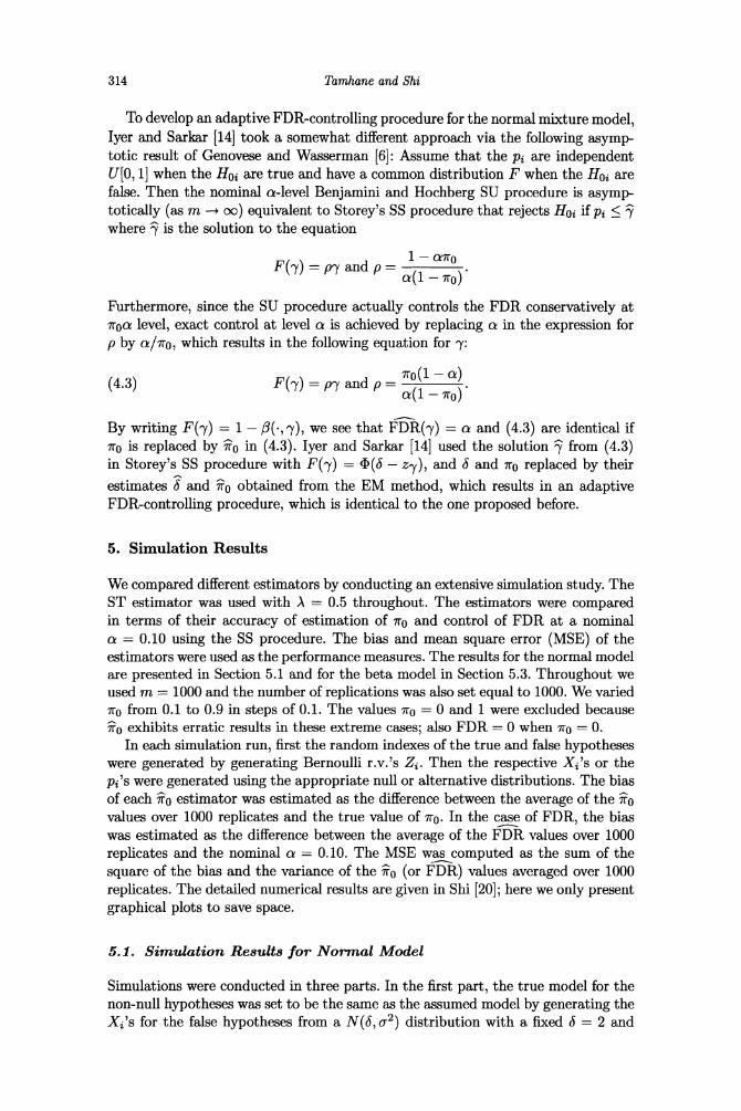
The bias and the square root of the mean square error (v'MSE) of ro for ST, HCK, TS and EM estimators are plotted in Figure 1. Note from equation (2.3) that the bias of the ST estimator is given by

1 - A (5.1) Bias[io(A)] = I(z4

- S). 1-AA

Also, using the fact that Na(A) has a binomial distribution with number of trials m and success probability,

p = P{pi > A} = -xo(1 - A) + (1 - 7ro) I(zA - 6),

and using equation (1.2) for 'ro(A), we have

p(1 -p) (5.2) Var[ro(A)]- = ) m(1 -

A)2

These formulae were used to compute the bias and MSE of the ST estimator instead of estimating them by simulation. Note that the bias of the ST estimator decreases linearly in

0ro. The v/MSE plot for the ST estimator is also approximately linear

because the bias is the dominant term in MSE. This is true whenever the alternative is fixed for all false null hypotheses.

The TS estimator does not offer an improvement over the HCK estimator, as we had hoped, and in fact performs slightly worse in terms of MSE for 7ro _

0.5. We sus- pect that this result is due to the bias introduced when the term E[Nr(A)]E[Xr(A)]

0.05 0.045

0.01

S0.0 EM s0.025 S0.015

-0.01 00.01 0.1 0.2 0.3 0.4 0.5 0.6 0.7 0.8 0.9 0.1 0.2 0.3 0.4 0.5 0.8 0.7 0.8 0.9

Xo Xo

FIG 1. Bias and VM7-- of 7o for ST, HCK, TS and EM Estimators for Normal Model (Data Generated by Normal Model with Fixed 6).

316 Tamhane and Shi

0.011 0.07

0 .0 0 5

0-

S T HCK

B- TS S0 EM

m 0.05 LL

-.005l

0.04

-0.020 0.03

-0.025 001 -0.082-- HCK B ETS 0.01

-0.03 0 0.1 02 0.3 0.4 0.5 0.6 0.7 0.8 0.9 0.1 0.2 0.3 0.4 0.5 0.6 0.7 0.8 0.9

Xo Xo

FIG 2. Bias and v/iAM of FDR for ST, HCK, TS and EM Estimators for Normal Model (Data Generated by Normal Model with Fixed 6).

in equation (2.12) is estimated by iXr(p(i)) for A = p(i) because of the fact that the product of the expected values does not equal the expected value of the product of two dependent r.v.'s. The EM estimator has consistently the lowest bias and the lowest MSE.

The bias and MSE of FDR for ST, HCK, TS and EM estimators are plotted in Figure 2. We see that the ST estimator leads to a large negative bias which means that, on the average, FDR is less than the nominal a = 0.10 resulting in conservative control of FDR. The other three estimators yield approximately the same level of control. Surprisingly, there is very little difference in the MSEs of the four estimators. The EM estimator still is the best choice with the lowest bias and the lowest MSE throughout the entire range of io values.

Results for Random 6

The bias and V/MSE of ro and of FDR for ST, HCK, TS and EM estimators are plotted in Figures 3 and 4, respectively. By comparing these results with those for fixed 6 = 2, we see that, as one would expect, there is a slight degradation in the

performance of every estimator because the assumed model does not hold. The

eHCK ST

0.04-- -TS I

0.045 -HCK

SEMI - TS

OF 0.04--- EM

So.oss 0.03

0.02 0- 0.02-

-4.01 000.015 1 0.1 0.2 0.3 0.4 0.5 0.6 0.7 0.8 0.9 0.1 0.2 0.3 0.4 0.5 0.6 0.7 0.8 0.9

FIG 3. Bias and VM-E of io for ST, HCK, TS and EM Estimators for Normal Model (Data Generated by Normal Model with Random 6).


0.0o1 o 0.07

0.005

O.0--

S S0ST

0 0-

cEM

-0.005

.

0.05

0.04 -0.0150

-10- ST V -2EHCK

- TSEM 0.02 -0.00.01

0.1 0.2 0.3 0.4 0.5 0.6 0.7 0.8 0.9 0.1 0.2 0.3 0.4 0.5 0.6 0.7 0.8 0.9

Xo 0

FIG 4. Bias and fM&S of FDR for ST, HCK, TS and EM Estimators for Normal Model (Data Generated by Normal Model with Random 6).

comparisons between the four estimators here are similar to those for fixed 6 with the estimators ranked as EM > HCK > TS > ST.

5.2. Robustness Results for Data Generated by Beta Model

The bias and v/MSE of 0ro

and of FDR for ST, HCK, TS and EM estimators are plotted in Figures 5 and 6, respectively. Looking at Figure 5 first, we see that the biases and MSEs of all four estimators are an order of magnitude higher compared to the normal model data which reflects lack of robustness.

It is interesting to note that the EM estimator is no longer uniformly best for estimating rro. In fact, the HCK estimator has a lower bias and MSE for 0.2 <7ro 0 0.7. The lack of robustness of the EM estimator is likely due to the strong dependence of the likelihood methods on distributional assumptions. On the other hand, for the least squares methods, the dependence on the assumed distribution is only through its first moment and hence is less strong. As far as control of FDR is concerned, there are not large differences between the proposed estimators. However, when 7ro = 0.9 the proposed estimators exceed the nominal FDR by as much as 0.05, while the ST estimator still controls FDR conservatively. In conclusion, the HCK estimator performs best for the middle range of r0o values.

0.3 0.22 -ST

-a- ST

e-- HCK 0.2 -E HCK 0.25 - TS ---- TS

S EM 0.18 EM

0.2 1 b 0.16

0.15 0.14

0.15

"B 0.1 0

S0.1

0.05- 0.08-

0.0& 0

0.04

01.060.01 0.1 0.2 0.3 0.4 0.5 0.6 0.7 0.8 0.9 0.1 0.2 0.3 0.4 0.5 0.6 0.7 0.8 0.9 Xo 0

FIG 5. Bias and VM&~ of 'o for ST, HCK, TS and EM Estimators for Normal Model (Data Generated by Beta Model).

318 Tamhane and Shi

0.06 I 1 0.22, , ,

--0.04 ST 0.2 --0--

ST 04 HCK ---- HCK S

TS 0.18 -B- TS 0.02 - EM --X EM

0.16

Z i 0.14 -0.02 0.12

-0 5 0U 0.1

0. -0.06 - 0.0

0.06

0.04

-0.1 .2 0.3 0.4 0.5 0.8 0.7

0.02 0.1 0.2 0.3 0.4 0.5 0.6 0.7 0.8 0.9 0.1 0.2 0.3 0.4 0.5 0.6 0.7 0.8 0.9

110 11

FIG 6. Bias and V 7K of FDR for ST, HCK, TS and EM Estimators for Normal Model (Data Generated by Beta Model).

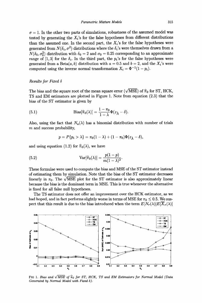
5.3. Simulation Results for Beta Model

Results for Beta(0.5, 2) Data

In this case the non-null p-values were generated from a Beta(a, b) distribution with a = 0.5, b = 2.0 and the null p-values were generated from the U[0, 1] distribution. As before, the bias and variance of the ST estimator were not estimated from simulations, but were computed using Equations (5.1) and (5.2) with ((zA -6) replaced by

1-Ia (a, b). Note that the bias of the ST estimator decreases linearly in ro in this

case as well and v/MSE decreases approximately linearly. From Figure 7 we see that all estimators of

0ro, except ST, have significant negative biases particularly over

the interval [0.2,0.5] and forr0 o > 0.7, resulting in the achieved FDR significantly exceeding the nominal value of a = 0.10 over the corresponding ranges of ro as can be seen from Figure 8. Comparing the results here with those for the normal model with the fixed 6 case, we see that the biases and MSEs of all estimators are an order of magnitude higher in the present case. The reason behind this poor performance of the beta model probably lies in the difficulty of estimating the parameters a, b of the beta distribution. Only the ST estimator controls FDR conservatively and has the smallest MSE for 0.2 < 7 o < 0.7. Thus the ST estimator has the best

-0- ST HCK 0.2-9- HCK

0.25- - TS -e- TS - EM 0.18 EM

0.2 0.16

0.15 0.14

0.1 S0.0812

0.05 00

0.06 0

0.04

0.1 0.2 0.3 0.4 0.5 0.6 0.7 0.8 0.9 0.1 0.2 0.3 0.4 0.5 0.6 0.7 0.8 0.9

Xo Xo

FIG 7. Bias and v/IAS of ^o for ST, HCK, TS and EM Estimators for Beta Model (Data Generated by Beta Model).


0.04 I I 0.18

0.10 E-T

0.12

-0.04 0.06 -0 ST -(-- HCK 0.06 -0.06 -BE- TS

0.04

-0.01 0. 1 0.1 0.2 0.3 0.4 0.5 0.8 0.7 0.8 0.9 0.1 0.2 0.3 0.4 0.5 0.8 0.7 0.8 0.9 0O X

FIG 8. Bias and VMH of FDR for ST, HCK, TS and EM Estimators for Beta Model (Data Generated by Beta Model).

performance since it is a nonparametric estimator (and the performance would be even better if A is not fixed, but is used as a tuning parameter). In other words, the benefits of using a parametric model are far outweighed by the difficulty of

estimating the parameters of the model resulting in less efficient estimators.

Robustness Results for Data Generated by Normal Model

In this case we generated the data by the normal model with N(2, 12) as the alternative distribution. The p-values were then computed and all four methods of estimation were applied. The results are plotted in Figures 9 and 10. From these figures we see that none of the proposed estimators exhibit consistent negative bias as they did when the data were generated according to the beta model. This is somewhat surprising since one would expect these estimators to perform more poorly when the assumed model does not hold as in the present case. We also see that the EM estimator performs worse than other estimators. Thus lack of robustness of the EM estimator to the model assumptions is demonstrated again, and for the same reason. The TS estimator generally has the lowest bias for estimating

0ro and

its achieved FDR is closest to the nominal a; the ST estimator has the second best performance.

0.08 0.13

-- - ST

E--)- HCK 0.12 --- ST

0 06 ----

TS -e- HICK X EM 0.11 ---B TS

0.02 0.08

0.08

Z006 cc 0.07

-0.02 0.06

0.05 -0.04

0.04

-0.01 0.031 0.1 0.2 0.3 0.4 0.5 0.6 0.7 0.8 0.9 0.1 0.2 0.3 0.4 0.5 0.0 0.7 0.8 0.9 0

FIG 9. Bias and VM7-S of ^o for ST, HCK, TS and EM Estimators for Beta Model (Data Generated by Normal Model).

320 Tamhane and Shi

0.0051 0 , 0.08

0 a-

ST

-00.07

- E HCK

- -0.01 -0.06 EM

B -0.015 i 0.05

EM 0.02 -0.042

-0.045 1

0.011 0.1 0.2 0.3 0.4 0.5 0.8 0.7 0.8 0.9 0.1 0.2 0.3 0.4 0.5 0.8 0.7 0.8 0.9 0o 0o

FIG 10. Bias and vH- of FDR for ST, HCK, TS and EM Estimators for Beta Model (Data Generated by Normal Model).

6. Example

We consider the National Assessment of Educational Progress (NAEP) data ana- lyzed by Benjamini and Hochberg [2]. The data pertain to the changes in the average eighth-grade mathematics achievement scores for the 34 states that participated in both the 1990 and 1992 NAEP Trial State Assessment. The raw p-values for the 34 states are listed in the increasing order in Table 2. The FWE controlling Bon- ferroni procedure and the Hochberg [9] procedure both identified only 4 significant results (those with p-values < P(4) = 0.0002) Application of the FDR controlling non-adaptive Benjamini-Hochberg SU procedure resulted in 11 significant results. By applying their method they estimated fio = 7

(0o = 0.2059); using this value

in the adaptive version of their procedure yielded 24 significant results. We applied the three methods of estimation considered in this paper to these

data under both the normal and beta models. The estimates ro and the associated J or (', b) values are given in Table 1. We see that for both models, the HCK and EM methods give smaller estimates of r0o than does the TS method. The '-values obtained by solving the equation FDR(-y) = a for a = 0.05 are inversely ordered.

The p-values < - are declared significant. From Table 2, we see that the number of significant p-values for HCK, TS and EM for the normal model are 28, 21 and

27, respectively. Thus, HCK and EM methods give more rejections than Benjamini and Hochberg's [2] adaptive SU procedure.

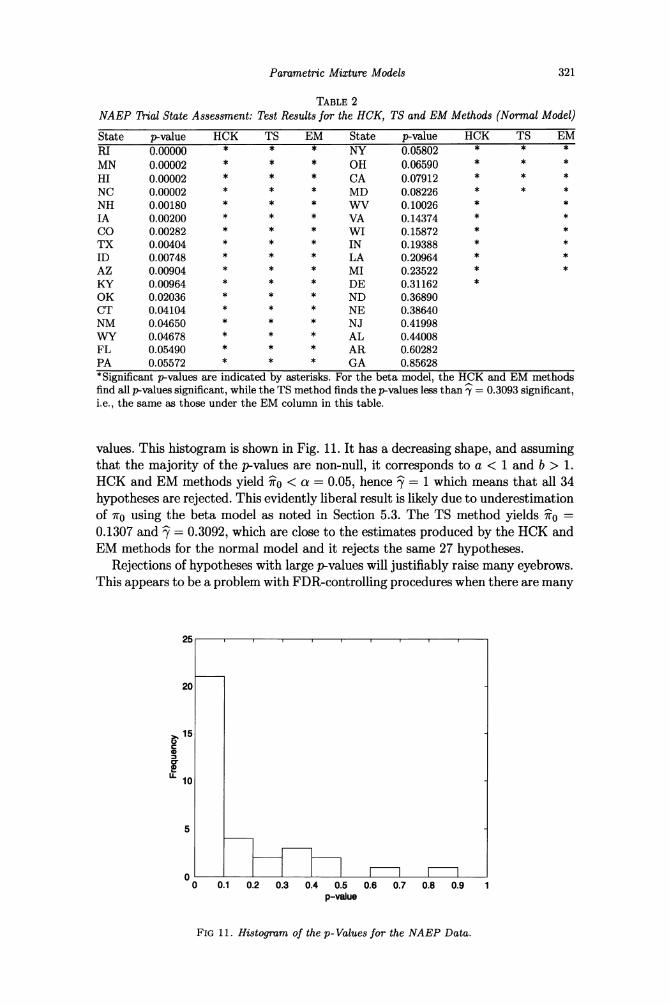
Before fitting the beta mixture model, it is useful to plot a histogram of the p-

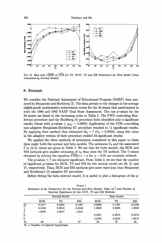
TABLE 1 Estimates of the Parameters for the Normal and Beta Models, Value of^ and Number of

Rejected Hypotheses for the HCK, TS and EM Methods

Normal Model Beta Model

HCK TS EM HCK TS EM

lro 0.1317 0.3233 0.1407 0.0096 0.1307 0.0160

7 0.3163 0.0918 0.2946 1.0000 0.3092 1.0000

6 1.8285 2.2657 1.9221 - - -

a- - - 0.3291 0.4474 0.3210

b - - - 2.0764 3.2842 1.9313 Nr 28 21 27 34 27 34 Nr = Number of rejected hypotheses.


TABLE 2 NAEP Trial State Assessment: Test Results for the HCK, TS and EM Methods (Normal Model)

State p-value HCK TS EM State p-value HCK TS EM RI 0.00000 * * * NY 0.05802 * * * MN 0.00002 * * * OH 0.06590 * * * HI 0.00002 * * * CA 0.07912 * * * NC 0.00002 * * * MD 0.08226 * * * NH 0.00180 * * * WV 0.10026 * * IA 0.00200 * * * VA 0.14374 * * CO 0.00282 * * * WI 0.15872 * * TX 0.00404 * * * IN 0.19388 * * ID 0.00748 * * * LA 0.20964 * * AZ 0.00904 * * * MI 0.23522 * * KY 0.00964 * * * DE 0.31162 * OK 0.02036 * * * ND 0.36890 CT 0.04104 * * * NE 0.38640 NM 0.04650 * * * NJ 0.41998 WY 0.04678 * * * AL 0.44008 FL 0.05490 * * * AR 0.60282 PA 0.05572 * * * GA 0.85628

*Significant p-values are indicated by asterisks. For the beta model, the HCK and EM methods find all p-values significant, while the TS method finds the p-values less than - = 0.3093 significant, i.e., the same as those under the EM column in this table.

values. This histogram is shown in Fig. 11. It has a decreasing shape, and assuming that the majority of the p-values are non-null, it corresponds to a < 1 and b > 1. HCK and EM methods yield ?ro < a = 0.05, hence ' = 1 which means that all 34 hypotheses are rejected. This evidently liberal result is likely due to underestimation of

0ro using the beta model as noted in Section 5.3. The TS method yields o0 =

0.1307 and ' = 0.3092, which are close to the estimates produced by the HCK and EM methods for the normal model and it rejects the same 27 hypotheses.

Rejections of hypotheses with large p-values will justifiably raise many eyebrows. This appears to be a problem with FDR-controlling procedures when there are many

25

20

15

10

5

0 0 0.1 0.2 0.3 0.4 0.5 0.6 0.7 0.8 0.9

p-value

FIG 11. Histogram of the p-Values for the NAEP Data.

322 Tamhane and Shi

hypotheses that are clearly false (with p-values close to zero) which lowers the bar for rejection for other hypotheses. Shaffer [19] has discussed this problem and has suggested imposing additional error controlling requirements in order to limit such dubious rejections. This is a topic for further research.

7. Concluding Remarks

In this paper we offered two different mixture models for estimating the number of true null hypotheses by modeling the non-null p-values. For each model (the normal and beta), three methods of estimation were developed: HCK, TS and EM. Gener- ally speaking, these parametric estimators outperform (in terms of the accuracy of the estimate of iro and control of the FDR) the nonparametric ST estimator for the normal model but not for the beta model. The reason for this is that the normal model is easier to estimate and so the benefits of the parametric estimators are not significantly compromised by the errors of estimation. On the other hand, the beta model is difficult to estimate and so the benefits of the parametric estimators are lost. Therefore we do not recommend the use of the beta model in practice.

For normally distributed test statistics, the EM estimator generally performs best followed by the HCK and TS estimators. However, the EM estimator is not robust to the violation of the model assumptions. If the EM estimator for the normal model is applied to the data generated from the beta model or vice versa, its performance is often worse than that of the HCK estimator, and sometimes even that of the ST estimator. The TS estimator did not improve on the HCK estimator in all cases as we had hoped. Thus our final recommendation is to use the normal model with the EM method if the test statistics follow approximately normal distributions and the HCK method otherwise. If only the p-values calculated from various types of test statistics are available then the ST method is recommended; alternatively the p-values may be transformed using the inverse normal transform and then the HCK method may be applied.

Appendix

Proof of Lemma 2. We have

E[Xa(A)>= E { Xi jiESa(A)

= E EXi So (A) = sa,Na (A) - na iEsa

= -E- na [g(~o, 6, A)COa(A) + [1 - g(l0o,

6, A)]Cla(6, A)]

= g(lro, 6, A)coa(A) + [1 - g(ro, 6, A )]cia(, A).

In the penultimate step above, we have used the fact that conditionally on Xi zA, the probability that Zi = 1 is g(lro, 6, A) and the probability that Zi = 0 is 1 - g(ro, 6, A). Furthermore, the conditional expectation of Xi in the first case is

C0a(A) and in the second case it is Cia(6, A). The expression for E[X,(A)] follows

similarly. O


Proof of Lemma 5. By substituting for 0(., 7) from (2.2) and dropping carets on

FDR(7), ro, ~Ii and 6 for notational convenience, the equation to be solved is

FDR(y) = 7

0ro + 71r (6- zy)/y

It is easy to check that FDR(0) = 0 and FDR(1) = r0o. We shall show that FDR(7) is an increasing function of y which will prove the lemma. Thus we need to show that u(6, y) = (D(6 - zy)/y is decreasing in 7. By implicit differentiation of the equation (I(zy) = 1 - y, we get

dzy 1

dy q(zy)

du(6, 7) _ y(6 - z7) - A(zy)4(6 - zy) dy 72A(zy)

Hence,

Therefore we need to show that

v(6, 7) = - zy) - Y7(6 - zy) > 0 V 6 > 0.

Now v(0, y) = 0. Therefore we must show that

dv(6, 7) db = q(6 - zy)[q(zy) + y(6 - zy)] > 0, d6

which reduces to the condition: w(6, y7) = (z7) + y(5 - zy) > 0. Since w(6, y) is increasing in 6, it suffices to show that

w (0, y) = A(zy) - yzy > 0.

By putting x = zy and hence 7 = ((-x) the above inequality becomes

4(-x) 1 ()<-, q$(x) x

which is the Mills' ratio inequality (Johnson and Kotz [16], p. 279). This completes the proof of the lemma. O

Proof of Lemma 6. By substituting for 3(., 7) from (3.2) and dropping carets on

FDR(y), o, 1i, a and b for notational convenience, the equation to be solved is

(A.1) FDR(7y) 7r 0ro + rlly (a, b)//y Note that FDR(0) = 0 and FDR(1) = 7ro. To show that FDR(y) is an increasing function of 7 we need to show that Iy(a, b)/7 decreases in y. To see this, note that the derivative of Iy(a, b)/7 w.r.t. y is proportional to yg(7ya, b) - Iy (a, b), which is negative since the beta p.d.f. g(yja, b) is strictly decreasing in 7 for a < 1 and b > 1, and so yg(71a, b) < Iy(a, b). It follows therefore that the equation FDR(7) = a has a unique solution in 7 E (0, 1) for a E (0, 7r0]. O-

324 Tamhane and Shi

Acknowledgments

This research was partially supported by the National Heart, Lung and Blood Institute Grant 1 R01 HL082725-01A1 and the National Security Agency Grant H98230-07-1-0068. The authors are extremely grateful especially to one of the two referees who pointed out some crucial errors in the earlier version of the paper.

References

[1] BENJAMINI, Y. and HOCHBERG, Y. (1995). Controlling the false discovery rate: A practical and powerful approach to multiple testing. J. Roy. Statist. Soc. Ser. B 57 289-300.

[2] BENJAMINI, Y. and HOCHBERG, Y. (2000). On the adaptive control of the false discovery rate in multiple testing with independent statistics. J. Educational Statist. 25 60-83.

[3] BLACK, M. A. (2004). A note on the adaptive control of false discovery rates. J. Roy. Statist. Soc. Ser. B 66 297-304.

[4] DEMPSTER, A. P., LAIRD, N. M. and RUBIN, D. B. (1977). Maximum likelihood from incomplete data via the EM algorithm. J. Roy. Statist. Soc. Ser. B 39 1-38.

[5] FINNER, H. and ROTERS, M. (2001). On the false discovery rate and expected type I error. Biom. J. 8 985-1005.

[6] GENOVESE, C. and WASSERMAN, L. (2002). Operating characteristics and extensions of the false discovery rate procedure. J. Roy. Statist. Soc. Ser. B 64 499-517.

[7] GILL, P. E., MURRAY, W. and WRIGHT, M. H. (1981). Practical Optimiza- tion. Academic Press, London and New York.

[8] GUAN, Z., Wu, B. and ZHAO, H. (2004). Model-based approach to FDR estimation. Technical Report 2004-016, Division of Biostatistics, Univ. of Min- nesota, Minneapolis, MN.

[9] HOCHBERG, Y. (1988). A sharper Bonferroni procedure for multiple tests of significance. Biometrika 75 800-803.

[10] HOCHBERG, Y. and BENJAMINI, Y. (1990). More powerful procedures for multiple significance testing. Statist. Med. 9 811-818.

[11] HOCHBERG, Y. and TAMHANE, A. C. (1987). Multiple Comparison Proce- dures. Wiley, New York.

[12] HSUEH, H., CHEN, J. J. and KODELL, R. L. (2003). Comparison of methods for estimating the number of true null hypotheses in multiple testing. Journal of Biopharmaceutical Statistics 13 675-689.

[13] HUNG, H. M., O'NEILL, R. T., BAUER, P. and KOHNE, K. (1997). The behavior of the p-value when the alternative hypothesis is true. Biometrics 53 11-22.

[14] IYER, V. and SARKAR, S. (2007). An adaptive single-step FDR procedure with applications to DNA microarray analysis. Biom. J. 49 127-135.

[15] JIANG, H. and DOERGE, R. W. (2005). Estimating the proportion of the true null hypotheses for multiple comparisons. Preprint.

[16] JOHNSON, N. L. and KOTZ, S. (1970). Continuous Univariate Distributions I. Wiley, New York.

[17] LANGAAS, M., LINDQUIST, B. H. and FERKINGSTAD, E. (2004). Estimating the proportion of true null hypotheses, with application to DNA microarray data. J. Roy. Statist. Soc. Ser. B 67 555-572.


[18] SCHWEDER, T. and SPJOTVOLL, E. (1982). Plots of p-values to evaluate many tests simultaneously. Biometrika 69 493-502.

[19] SHAFFER, J. P. (2005). Multiple requirements for multiple test procedures. Paper presented at the IVth International Conference on Multiple Comparison Procedures, Shanghai, China.

[20] SHI, J. (2006). Improved Estimation of the Proportion of True Null Hypotheses with Applications to Adaptive Control of FDR and Drug Screening. Doctoral dissertation, Department of Statistics, Northwestern University, Evanston, IL.

[21] STOREY, J. (2002). A direct approach to false discovery rates. J. Roy. Statist. Soc. Ser. B 64 297-304.

[22] STOREY, J., TAYLOR, J. E. and SIEGMUND, D. (2004). Strong control, conservative point estimation and simultaneous conservative consistency of false discovery rates: A unified approach. J. Roy. Statist. Soc. Ser. B 66 187-205.

[23] TURKHEIMER, F. E., SMITH, C. B. and SCHMIDT, K. (2001). Estimation of the number of 'true' null hypotheses in multivariate analysis of neuroimaging data. Neurolmage 13 920-930.

[24] Wu, B., GUAN, Z. and ZHAO, H. (2006). Parametric and nonparametric FDR estimation revisited. Biometrics 62 735-744.

Documents

Parametric Mixture Models for Estimating the Proportion of ...users.iems.northwestern.edu/~ajit/papers/45) FDR Paper.pdf · model assumes that the test statistics from the true null