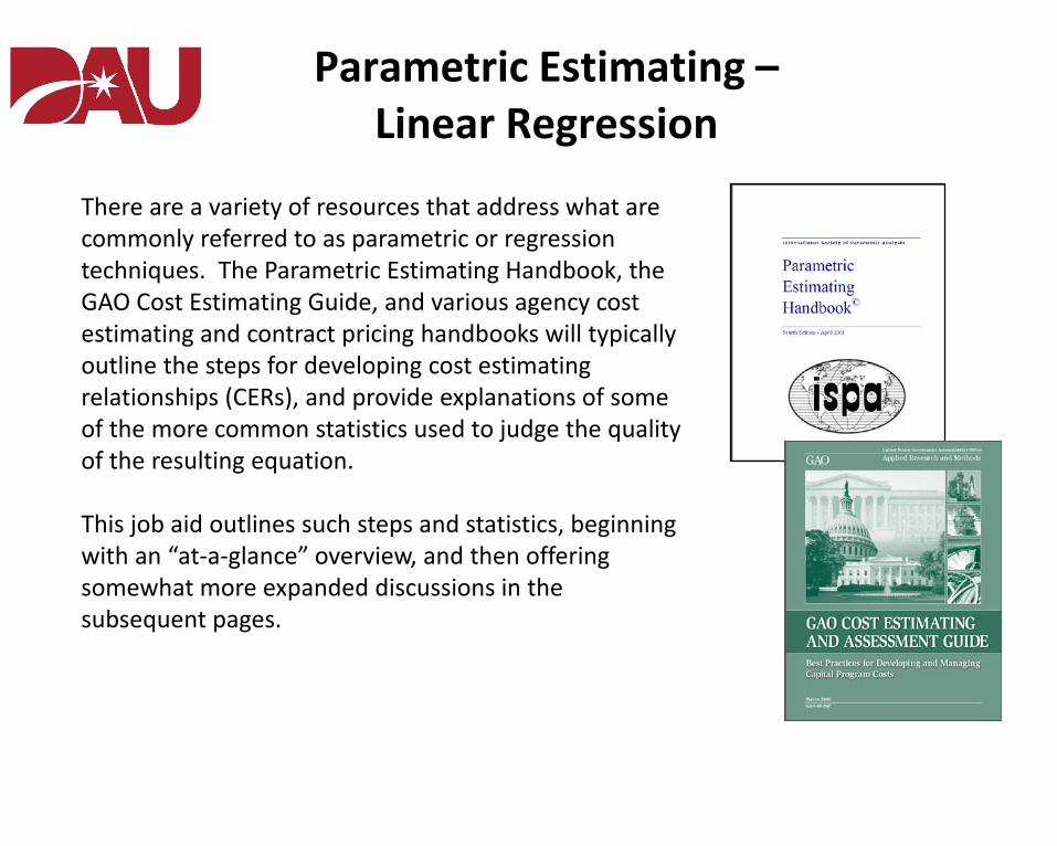
Parametric Estimating –Linear Regression

There are a variety of resources that address what are commonly referred to as parametric or regression techniques. The Parametric Estimating Handbook, the GAO Cost Estimating Guide, and various agency cost estimating and contract pricing handbooks will typically outline the steps for developing cost estimating relationships (CERs), and provide explanations of some of the more common statistics used to judge the quality of the resulting equation.

This job aid outlines such steps and statistics, beginning with an “at-a-glance” overview, and then offering somewhat more expanded discussions in the subsequent pages.

Developing Cost Estimating Relationships

Developing Cost Estimating Relationships

Developing Cost Estimating Relationships

The term “cost estimating relationship” or CER is used here in the context of an equation where we predict the outcome of one variable as a function of the behavior of one or more other variables.

We refer to the predicted variable as the dependent or Y variable. Those variables that can be said to explain or drive the behavior of the predicted variable are consequently called explanatory variables or cost drivers, also known as the independent or X variables.

The terms CERs, equations, or models are often used interchangeably, although the term “model” is sometimes reserved to describe an assemblage of CERs, equations, or factors such as is often the case with respect to a software cost estimating “model”.

Developing Cost Estimating Relationships

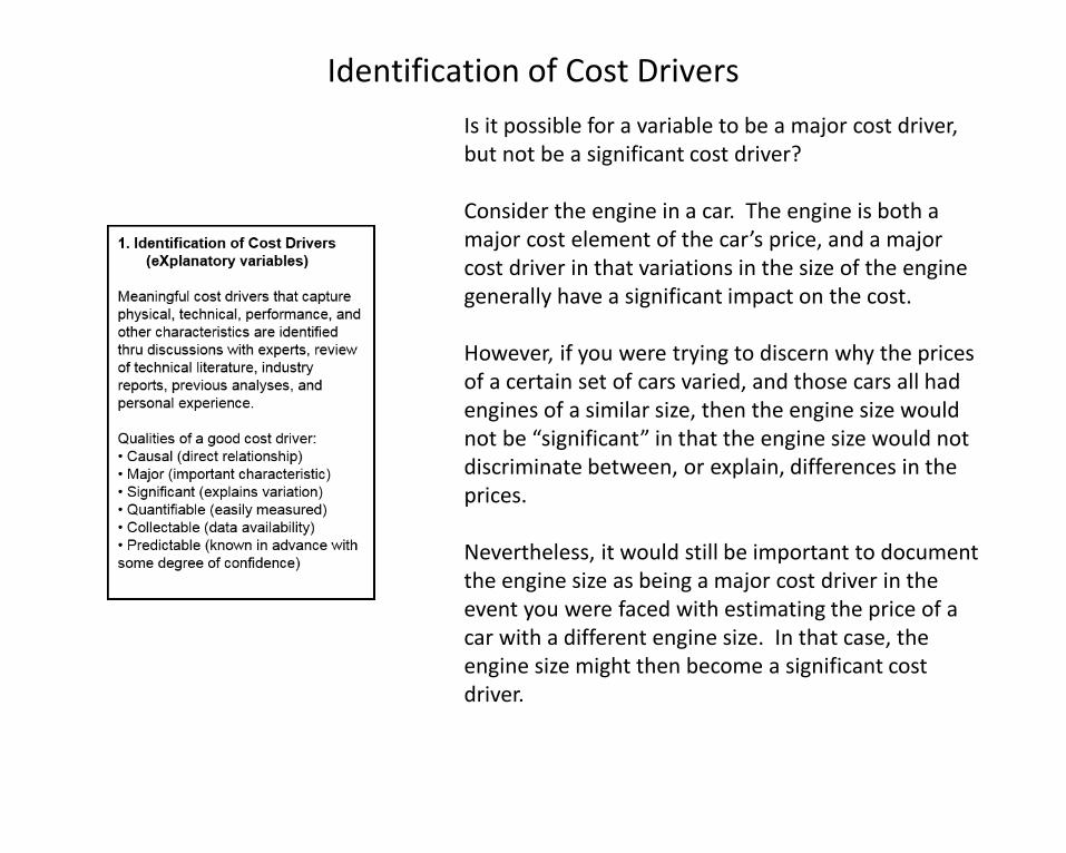
Is it possible for a variable to be a major cost driver, but not be a significant cost driver?

Consider the engine in a car. The engine is both a major cost element of the car’s price, and a major cost driver in that variations in the size of the engine generally have a significant impact on the cost.

However, if you were trying to discern why the prices of a certain set of cars varied, and those cars all had engines of a similar size, then the engine size would not be “significant” in that the engine size would not discriminate between, or explain, differences in the prices.

Nevertheless, it would still be important to document the engine size as being a major cost driver in the event you were faced with estimating the price of a car with a different engine size. In that case, the engine size might then become a significant cost driver.

Identification of Cost Drivers

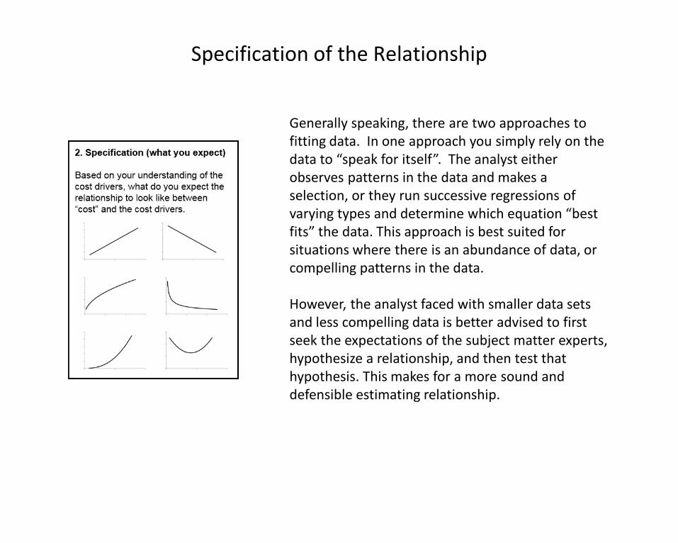
Generally speaking, there are two approaches to fitting data. In one approach you simply rely on the data to “speak for itself”. The analyst either observes patterns in the data and makes a selection, or they run successive regressions of varying types and determine which equation “best fits” the data. This approach is best suited for situations where there is an abundance of data, or compelling patterns in the data.

However, the analyst faced with smaller data sets and less compelling data is better advised to first seek the expectations of the subject matter experts, hypothesize a relationship, and then test that hypothesis. This makes for a more sound and defensible estimating relationship.

Specification of the Relationship

One challenge that analysts sometimes face is a shortage of similar items for comparison. When searching for “similar” items, the analyst should consider the level at which that similarity need exist. For example, an analyst pricing a component on a stealth ship need not unnecessarily constrain themselves to stealth ships when it is possible that the same or similar component is used on a variety of ships, and perhaps ground vehicles and aircraft as well.

Another consideration for expanding the number of similar items is to estimate at lower levels of the work breakdown structure when necessary, and when such data exists.

Familiarize yourself with the data bases that your organization and others maintain.

Data Collection

You probably learned at some point in a science class that when constructing experiments to study the effects of one thing upon another that it was important to hold everything else constant as much as possible. That’s essentially the idea behind normalizing the data, to get a more true measure of the relationship between the Y and X variables.

One of the other benefits of going through the process of making these adjustments in the data is that it forces us to develop a better understanding of the effects that each of these factors has on “cost”, such as the changes in quantity, technology, material, labor differences, etc.

Look for checklists that your agency and others use when comparing prices, costs, hours, etc.

Normalizing the Data

If you’re counting on the R2, T statistic, F statistic, standard error, or coefficient of variation to tell you that you are not properly fitting the data, or that you have outliers or gaps in the data, then get ready to be disappointed, because they won’t!

Histograms, number lines, scatterplots, and more. There is just no substitution for looking at the data.

Hopefully the scatterplots will be consistent with your expectations from the specification step. If not, then this is the opportunity to reengage with your subject matter experts.

Scatterplots may highlight subgroups or classes within the data; changes in the cost estimating relationship over the range of the data; and unusual values within the data set.

Graphical/Visual Analysis of the Data

This step is the extension of the specification and visual analysis steps. We will concern ourselves here with linear relationships. See the Nonlinear job aid for discussions on fitting nonlinear data.

The most common linear relationship is a factor. The use of a factor presumes a direct proportional relationship between the X and Y variables.

A factor can be derived from a single data point or from a set of data points. Regression can be used to derive a factor when dealing with a set of data points by specifying a zero intercept or “constant is zero” in applications such as Excel. (See the Factors job aid for further discussion on the use of factors.)

Selecting a Fitting Approach for the Data

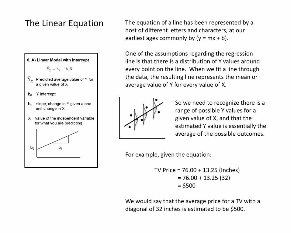
The equation of a line has been represented by a host of different letters and characters, at our earliest ages commonly by (y = mx + b).

One of the assumptions regarding the regression line is that there is a distribution of Y values around every point on the line. When we fit a line through the data, the resulting line represents the mean or average value of Y for every value of X.

For example, given the equation:

TV Price = 76.00 + 13.25 (Inches) = 76.00 + 13.25 (32) = $500

We would say that the average price for a TV with a diagonal of 32 inches is estimated to be $500.

So we need to recognize there is a range of possible Y values for a given value of X, and that the estimated Y value is essentially the average of the possible outcomes.

The Linear Equation

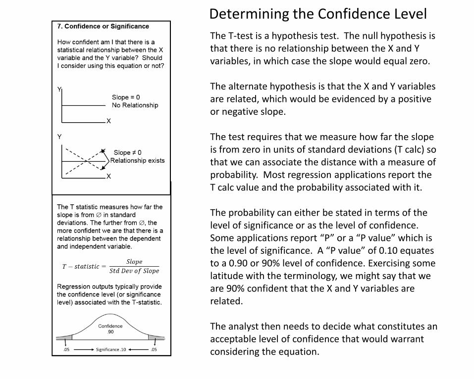
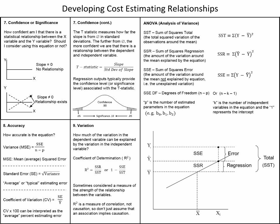
The T-test is a hypothesis test. The null hypothesis is that there is no relationship between the X and Y variables, in which case the slope would equal zero.

The alternate hypothesis is that the X and Y variables are related, which would be evidenced by a positive or negative slope.

The test requires that we measure how far the slope is from zero in units of standard deviations (T calc) so that we can associate the distance with a measure of probability. Most regression applications report the T calc value and the probability associated with it.

The probability can either be stated in terms of the level of significance or as the level of confidence. Some applications report “P” or a “P value” which is the level of significance. A “P value” of 0.10 equates to a 0.90 or 90% level of confidence. Exercising some latitude with the terminology, we might say that we are 90% confident that the X and Y variables are related.

The analyst then needs to decide what constitutes an acceptable level of confidence that would warrant considering the equation.

Determining the Confidence Level

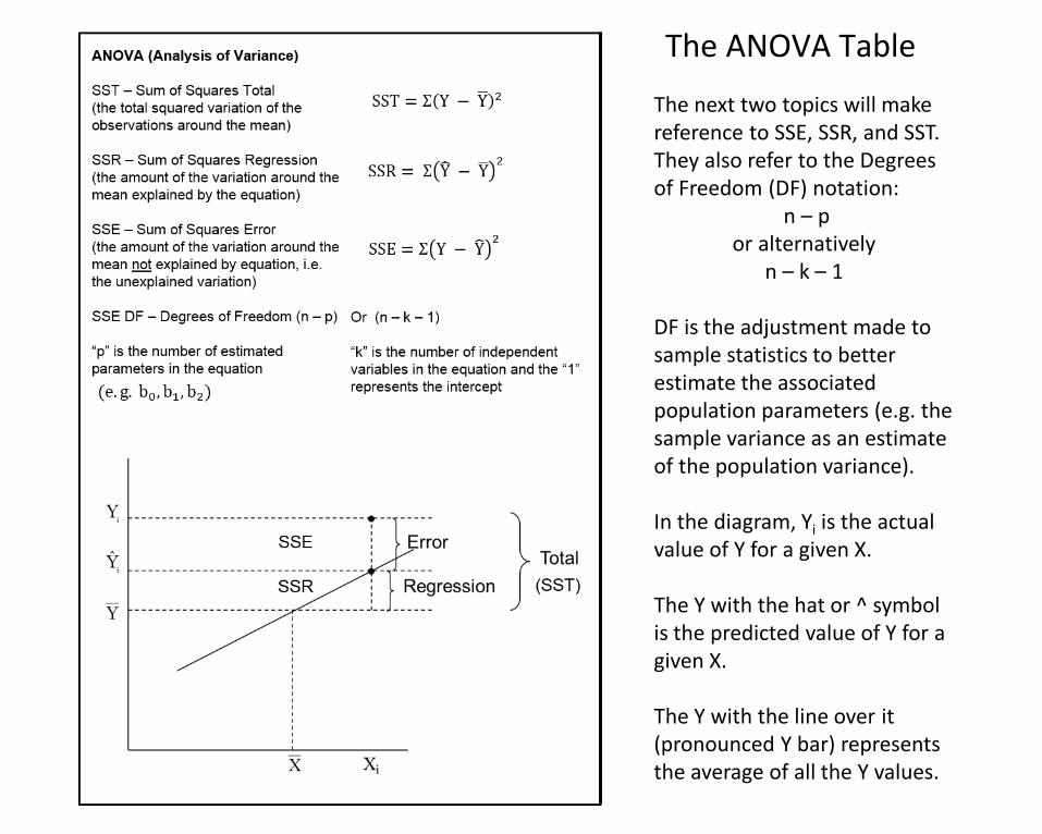
The next two topics will make reference to SSE, SSR, and SST. They also refer to the Degrees of Freedom (DF) notation:

n – p or alternatively

n – k – 1

DF is the adjustment made to sample statistics to better estimate the associated population parameters (e.g. the sample variance as an estimate of the population variance).

In the diagram, Yi is the actual value of Y for a given X.

The Y with the hat or ^ symbol is the predicted value of Y for a given X.

The Y with the line over it (pronounced Y bar) represents the average of all the Y values.

The ANOVA Table

Ideally we would test the accuracy of the equation by reserving some of the data points, and then assessing how well we estimated those points based on the equation resulting from the remaining data.

Unfortunately, due to the far too common problem of small data sets we cannot afford the luxury of reserving data points. As an alternative, we measure how well we fit the data used to create the equation.

The SSE is the sum of the squared errors around the regression line. By dividing the SSE by “n – p” or alternatively by “n – k – 1”, we arrive at the variance of the equation, and what we might loosely call the average squared estimating error.

The square root of the variance is commonly called the standard error or standard error of the estimate. Again, we could loosely interpret this as the average estimating error.

By comparing the standard error to the average value of Y we get a relative measure of variability called the coefficient of variation, which we might think of as an average percent estimating error.

How Accurate is the Equation?

Presumably we are developing a CER to explain the variation in our Y variable for the purpose of better estimating it. It seems reasonable then to ask how much of the variation in the Y variable that we have been able to account for.

The sum of squares total, or SST, represents the total squared variation around the mean of Y. The sum of squares regression, or SSR, represents the portion of the variation in the SST that we have accounted for in the equation. You might say SSR is the variation in Y that we can associate with the variation in X.

R squared is the ratio of the explained variation (SSR) to the total variation (SST). While calculated as a decimal value between 0 and 1, it’s commonly expressed as a percentage between 0 and 100. If the equation bisected all of the data points, R squared would be 100%, meaning all of the variation in Y would have been explained by the variation in X.

R squared should not be used to imply causality, but rather used to support the causality supposition from the step where we identified what we believed to be causal cost drivers.

How much of the variation in Y has been

explained?

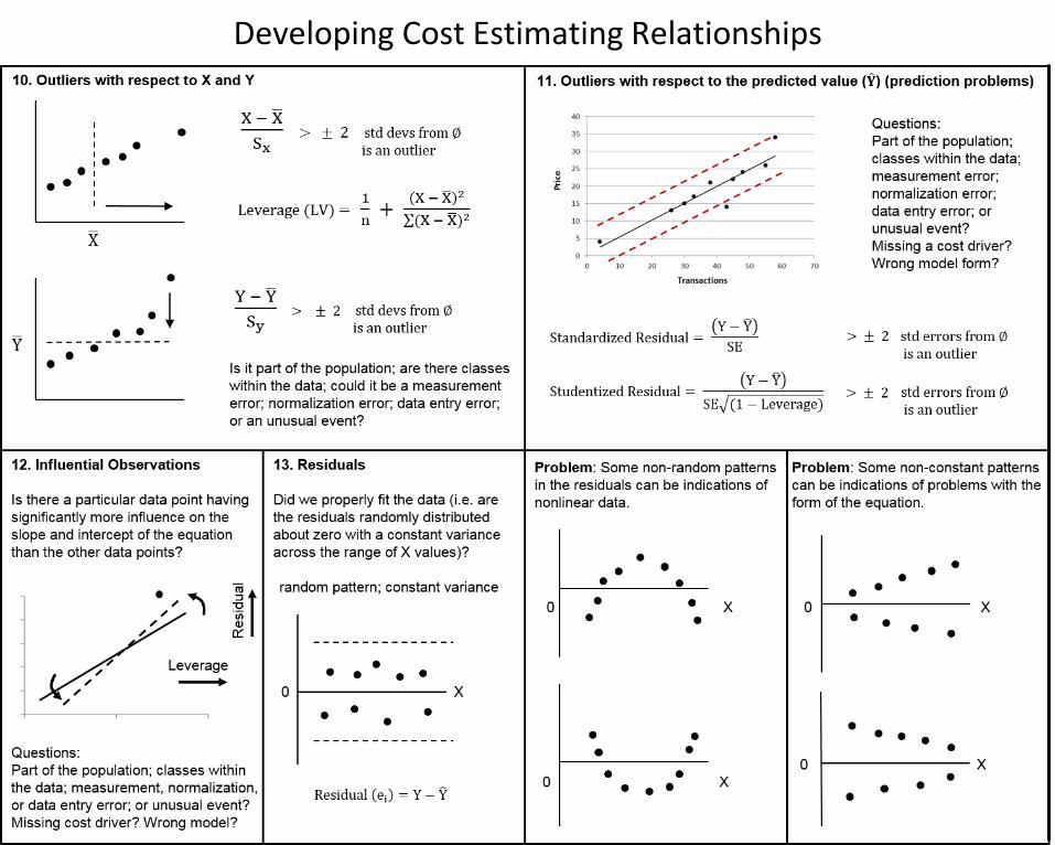
We want to be aware of unusual values in the data for a number of reasons. It may indicate deficiencies in how we’ve normalized the data. It could be that there are differences in the data that either we were unaware of, or if we were aware of, we didn’t know the impact those differences would have. And there is the concern of how that unusual value impacts our ability to fit the remaining data.

One test for what we call outliers, is to measure how far an X or Y value is from the mean of X or Y, in units of standard deviations. A more robust technique for the X variable is to calculate the leverage value for each X. Well-named, the higher the leverage value, the more leverage a particular X data point has on the slope and intercept of the equation. Outliers should be investigated prior to consideration for removal from the data set.

When does an X or Y become an outlier? It’s subjective, but one convention is that when a value is more than plus or minus two standard deviations from the mean it is considered an outlier.

Leverage uses P (the number of coefficients in the equation) divided by “n” (the sample size). A multiplier of 2 or 3 times P/n is used as the point at which an X observation becomes an outlier.

X and Y Outliers

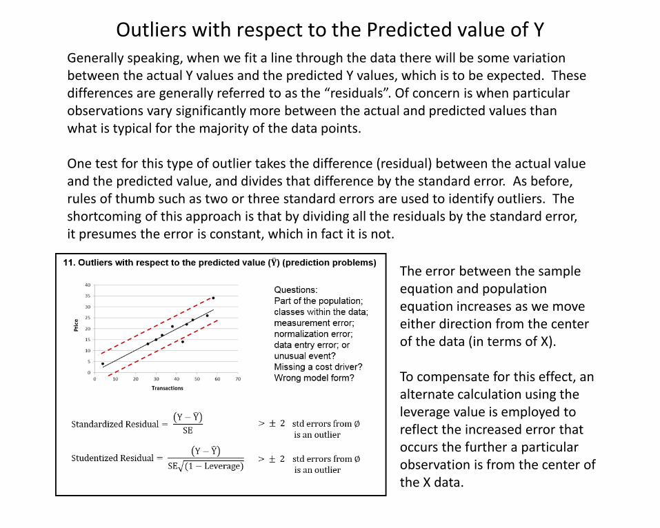
Generally speaking, when we fit a line through the data there will be some variation between the actual Y values and the predicted Y values, which is to be expected. These differences are generally referred to as the “residuals”. Of concern is when particular observations vary significantly more between the actual and predicted values than what is typical for the majority of the data points.

One test for this type of outlier takes the difference (residual) between the actual value and the predicted value, and divides that difference by the standard error. As before, rules of thumb such as two or three standard errors are used to identify outliers. The shortcoming of this approach is that by dividing all the residuals by the standard error, it presumes the error is constant, which in fact it is not.

The error between the sample equation and population equation increases as we move either direction from the center of the data (in terms of X).

To compensate for this effect, an alternate calculation using the leverage value is employed to reflect the increased error that occurs the further a particular observation is from the center of the X data.

Outliers with respect to the Predicted value of Y

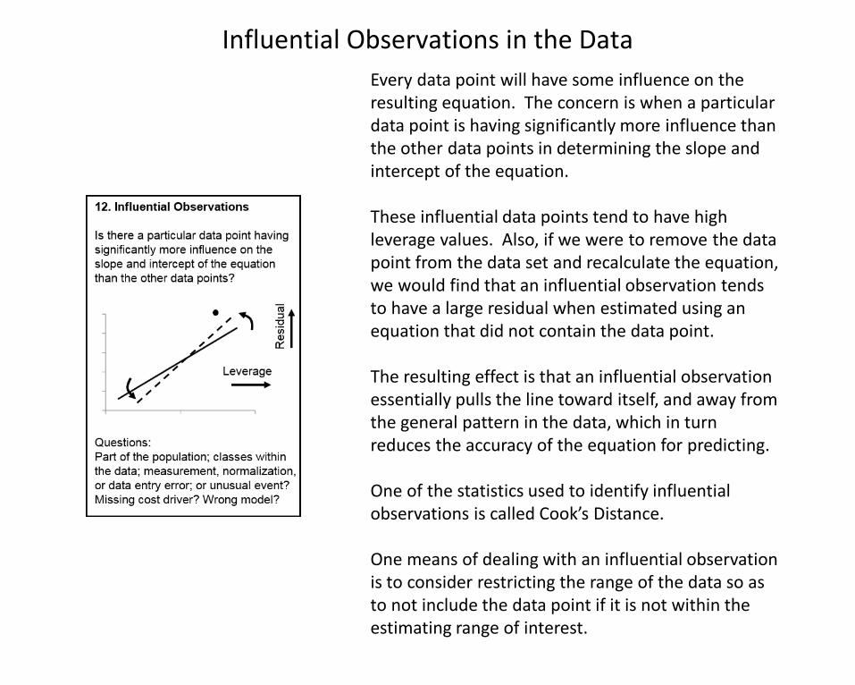
Every data point will have some influence on the resulting equation. The concern is when a particular data point is having significantly more influence than the other data points in determining the slope and intercept of the equation.

These influential data points tend to have high leverage values. Also, if we were to remove the data point from the data set and recalculate the equation, we would find that an influential observation tends to have a large residual when estimated using an equation that did not contain the data point.

The resulting effect is that an influential observation essentially pulls the line toward itself, and away from the general pattern in the data, which in turn reduces the accuracy of the equation for predicting.

One of the statistics used to identify influential observations is called Cook’s Distance.

One means of dealing with an influential observation is to consider restricting the range of the data so as to not include the data point if it is not within the estimating range of interest.

Influential Observations in the Data

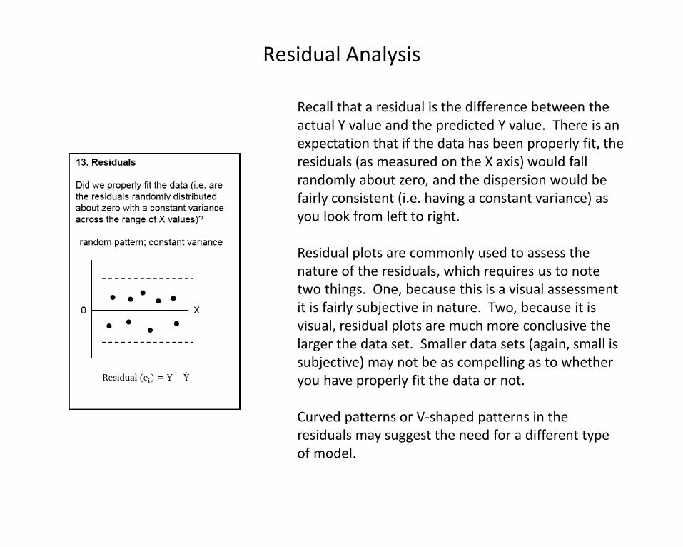
Recall that a residual is the difference between the actual Y value and the predicted Y value. There is an expectation that if the data has been properly fit, the residuals (as measured on the X axis) would fall randomly about zero, and the dispersion would be fairly consistent (i.e. having a constant variance) as you look from left to right.

Residual plots are commonly used to assess the nature of the residuals, which requires us to note two things. One, because this is a visual assessment it is fairly subjective in nature. Two, because it is visual, residual plots are much more conclusive the larger the data set. Smaller data sets (again, small is subjective) may not be as compelling as to whether you have properly fit the data or not.

Curved patterns or V-shaped patterns in the residuals may suggest the need for a different type of model.

Residual Analysis

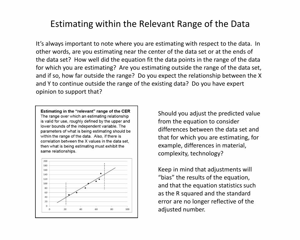
It’s always important to note where you are estimating with respect to the data. In other words, are you estimating near the center of the data set or at the ends of the data set? How well did the equation fit the data points in the range of the data for which you are estimating? Are you estimating outside the range of the data set, and if so, how far outside the range? Do you expect the relationship between the X and Y to continue outside the range of the existing data? Do you have expert opinion to support that?

Should you adjust the predicted value from the equation to consider differences between the data set and that for which you are estimating, for example, differences in material, complexity, technology?

Keep in mind that adjustments will “bias” the results of the equation, and that the equation statistics such as the R squared and the standard error are no longer reflective of the adjusted number.

Estimating within the Relevant Range of the Data