1

Parallel Software &Parallel Software &Parallel Programming LanguageParallel Programming Language

Dr. Stephen TseDr. Stephen Tse

stephen_tse@qc.edu

Lesson 6Lesson 6

2

Current Status of Parallelization

• Parallel processing technology has attracted attention in widespread fields

• This technology means the computer-structuring technology aimed at increasing the calculation speed by performing the process while running plural calculating function at the same time.

• The last 40 years of research is emphasized on hardware aspect – how to connect the processors and how to make the high-speed memory accessible.

• Such hardware end up in a failure to effectively improve actual program efficiency.

• The emphasis of the latest 10 years has been shifted to the software research for good use of the hardware.

3

The New Parallel Processing Format

• In practical use like the calculating pipeline format utilized in some supper computer leads to the recognition.

• The parallelizing software plays a significant role in narrowing the gap between the very high performance and the average performance machines.

• The Gflops machine which executes 109 time floating-decimal point calculation per second can be achieved by a cluster of average performance PCs.

• The second situation provides an environment which makes the use easy even for users other than experts on the parallel processing.

4

Two Categories on the Parallelizing Software

• Depending on the research approach, parallelizing software can be grossly classified into two categories:

1. First category represented by the development of the programming language for parallelization;

2. Concerning the research on the development of parallelizing compiler.

5

Programming Language for Parallelization

– the language related research to see how to express the parallelism problems

– how to make reflection of the user’s knowledge about the division of a program in the parallel processing function,

– Allotment to the processors and decision on execution sequence (scheduling) and others.

6

Parallelizing Compiler

• The compiler forms the parallelizing code based on the results of the scheduling on the processors

• Extract the parallelism in the program and schedule the parallel-based executable parts on the processors for minimizing the processing time

• Analyzing the flow of program data written in the sequential type languages and the flow of control (condition ramifications, etc.)

• Converting automatically to a form in which the parallel-based executable parts can be detected or the program can be processed in parallel (restructuring).

7

Expansion of Parallelizing in Sequential Language

• Research on sequential languages for parallel descriptions; e.g. Fortran, C, C++, etc…

• Conversational style tuning between the compilers and users is intended to make it possible to parallelize by taking advantage of the user’s knowledge, the parts which cannot be parallelized merely by program analysis of the compiler.

• The systematic two-sided research of user and compiler is important.

• Of these two side:– Research on optimizing parallel compiler for improving the

effective performance of the system and– Providing an environment that can be used in the same sense

as the conventional sequential computers environment without imposing any extra burden on the users

8

Parallelizing User EnvironmentUsers

Sequential languageFortran, C, C++PascalCray FortranPrologPCFFortran 99

Parallel type languages

Occam Data flowConcurrent Pascal languageGHCLinda

Parallelizing Compiler Parallelism extraction partData control dependence analysisProgram conversionGranularity determination

Task scheduling (static)

Parallel processing hardware Noiman type Non-Noiman type Vector processor Data flow Machine Multiprocessor system VLIW (Dynamic scheduling) OS run time system

Conversation

style

tuning

debug

Formation of parallelization machine code

Relations of parallel processing software: (1) The research on the parallelizing compilers which are intended to automatically find for process the parallelism from the conventional type of sequential languages and

(2) The research on the parallel languages concerning the question as to how the users should describe the parallelism for free use of the parallel processing hardware.

9

Conventional Parallel Extraction Technology• The compilers centered around the vectorizers for

pipeline formatted super computers.• The calculation pipeline format is aimed at achieving a

high-speed process in repeating the same calculations of different data like the arrangement calculation

• In the calculation of one-dimensional real number array A(I) and B(I), each consisting of N-numerated elements, are added to obtain the result C(I).

• This format is to replace the DO Loops expressing this with one-vector instruction for adding two vectors in the length of N as

C(1:N)=A(1:N) +B(1:N) Vectorization and processing such instruction in high

speed.• This process of the vector instructions allows a clock-by-

clock calculation results to be obtained in a steady state.

10

Calculating Pipelines

• The elements A(I) and B(I) following the floating-decimal point summing pipe divided in plural stages.

• If N (vector length) is long enough the calculations can be implemented using the time of 1/(number of stages) of the sequential process.

• Such calculation pipeline are adopted by many super computers, such as CRAY-1, CDC’s Cyber 205, Fujitsu’s VP400, Nichiden’s SX2, and Hitachi’s S820.

• The maximum performance of a single vector processor are 4GFlops of Fujitsu’s VP2000 and 5.5 GFlops of Fujitsu’s SX-3.

• The calculation pipeline format are also implemented with pipe chaining with multi-pipeline format.

… A(7) A(6)… B(7) B(6)

A(5) A(4)B(5) B(4)

A(3) +B(3)

C(2) C(1)

Indexical parts Digital Addition Regularizationcomparison coordination

The Calculation Pipeline Format: the calculating functions are divided into plural partial calculators which are set to operate in parallel with the process of flowing the data from the left end and taking it our from the right end on the unit time basis.

11

Basic Vectorization

• In the automatic parallelization, the compiler first conduct the analysis of the data dependence between instructions and between statements.

• The data dependence analysis is the most basic program analyses for the extraction of parallelism.

• The restraints related to execution sequence • Deriving from the definition and use of the data

between statements and others.

12

Kinds of Data Dependence

1. The flow dependence – the variable (data) defined by one statement is used by another statement;

2. The output dependence – the variable defined by one statement is re-defined by another statement; and

3. Counter-dependence = the variable used by one statement is defined by another statement.

13

Data Dependence Statements

• The Data Dependence relations mean the restrictions related to the execution sequence between statements,

• derived from the definition and use of data• The Flow dependence means S2’s use of the value of

Variable A is defined by S1.• The Output dependence means S3’s redefinition of the

value of variable A is defined by S1• The Counter dependence representsS4’s definition of

the value of Variable B used by S1.

A=B+C : S1D=A+E : S2A=C+F : S3B=E+F : S4

Flow dependence O Output A Counter

Dependence Dependence

14

Data Dependence Graph

• Data dependence between statements in the innermost of the DO Loop is examined,

• a data dependence graph is examined for absence of the cycle (or upward edge) in the graph to decide whether or not vectorization is possible.

• When there is an upward edge which does not form a loop, i.e. from S3 to S2. Vecctorization can be attained by exchanging the sequences of S3 and S2.

do I=2,N C(I)=A(I)+B(I) : S1 D(I)=C(I)+A(I-1) : S2 E(I)=D(I+1)+X : S3 A(I)=D(I)*B(I) : S4end do

S1

S2

S3

S4

C(2:N)=A(2:N)+B(2:N) : S1E(2:N)=D(3:N+1)+X : S3do I=2,N D(I)=C(I)+A(I-1) :S2 A(I)=D(I)*B(I) :S4end do

(a) Example of the Do Loop (B) Data dependence graph (c) Vectorized code

Example of Automatic vectorization

1. The statements in Do Loop (a) have a data dependence as shown in data dependence graph in (b).

2. The path from S1 to S2 represents only a downward edge and the S1 part can be replaced by the vector instruction in (c).

3. S2 and S4 have a flow interdependence between them and making up a loop; therefore cannot be vectorized.

4. The part from S3 to S2 has a counter dependence but the edge can be made to point downward by reversing the

sequence of S3 and S2. Therefore, S3 can be vectorized.

15

Data Dependence Analysis

• Presence of a cycle in the data dependence graph usually denies vectorization, but if one of the edges forming a cycle is counter-dependent or output-dependent, the compiler may perform the vectorization by inserting the substitution statement into the temporary arrangement.

do I=1,N do I=I,N C(I)=A(I)+B(I) TEMP(I)=C(I+1) TEMP(1:N)=C(2:N+1) D(I)=C(I)+C(I+1) C(I)=A(I)+B(I) C(1:N)=A(1:N)+B(1:N)end do D(I)=C(I)+TEMP(I) D(1:N)=C(1:N)+TEMP(1:N) end do

(a) This do loop having a cycle consisting of the flow dependence and counter-dependence

(b) This do loop can be rewritten by introducing the temporary variable of TEMP(I)

(c) Finally, it can be vectorized

16

SoftwareParallel Programming Language

Observation 1: A regular sequential programming language (C or Fortran or C++ etc) plus four communication statements (send, receive, myid, numnodes) are necessary and sufficient to form a parallel computing language.

1. Send: One processor sends a message to the network. Note this processor

does not have to know to which processor it is sending this message, but it does give “name” for the message.

2. Receive: One processor receives a message from the network. Note this

processor does not have to know which processor sends this message, but it retrieves the message by name.

3. myid: Integer between 0 and P-1 identifying a processor. myid is always

unique within one partition. 4. numnodes: Integer showing the total number of nodes in the system.

17

Send and Receive

Figure 1: Basic Message PassingSender: The circle on the left represents the "Sender" whose responsibility is to send a

message to the "Network Buffer” without knowing who is the receiver. Receiver: The “Receiver” on the right has to issue a message to the “buffer” to retrieve a

message that is labeled for it. Note:1. This is the so-called single-sided message passing, which is popular in most distributed-memory

supercomputer. 2. The Network Buffer as labeled, in fact, does not exist as an independent entity and is only a

temporary storage. It created either in the sender’s RAM or in the receiver’s RAM and depended on the readiness of the message routing information. For example, if a message’s destination is known but the exact location is not known at the destination, the message will be copied to the receiver’s RAM for easier transmission.

Sender

Network Buffer

Receiver

Figure 1: The basic concept of message passing.

18

THREE WAYS TO COMMUNICATE

1. Synchronous: The sender will not proceed to the next task until the

receiver retrieves the message from the network (hand deliver: slow!)

2. Asynchronous: The sender will proceed to the next task whether the

receiver retrieves the message from the network or not (mailing a letter: will not tie up sender!) No protection for the message in the buffer.

One example for Asynchronous message passing3. Interrupt: The receiver interrupts the sender's current activity for

pulling messages from the sender (ordering a package: interrupt sender!)

19

Synchronous Communication

Figure 2: Synchronous Message Passing

The circle on the left sends a message-1 to the imaginary Network “Buffer”, which then requests the destination to stop its current activities and ready to receive a message from the sender. In synchronous mode, the Receiver will immediately halt its current processing stream by issuing an acknowledgement to the Sender saying “OK” to send the message. After receiving this message, the Sender will immediately dump the original intended message to the Receiver at the exact location.

Send (msg 1)

Receivemsg 1

Figure 2: Synchronous Message Passing

msg 1Yes ?

OK ?

20

Asynchronous Communication

Figure 3: Asynchronous message passing: The Sender issues a message with the appropriate addressing header (envelope information) and regardless of the arrival of the message at the Receiver end or not, the Sender continues its execution without waiting for any confirmation from the Receiver. The Receiver, on the other hand, will also continue its own execution stream until the “receive” statement is met.

Note: The advantage with the asynchronous message passing is its speed. There is no need for either party to wait. The risk lies in the misuse of the correct message.

Send (msg 1)

Receivemsg 1

Figure 3: Asynchronous Message Passing

msg 1Yes ?

OK ?

21

Asynchronous MP ExampleAsynchronous Message Passing Example

SRC Processor (Sender) DST Processor (Receiver)

doing_something_useful……msg_sid=isend() /* send msg */……doing_sth_without_messing_msg

msg_rid=irecv() /* no need of msgs */…doing_sth_without_needing_msgs…msgwait(msg_rid); /*not return until msg arrives*/doing_sth_using_msgs

Choice II: msg_doneif (msgdone(msg_rid))doing_sth_with_it:else doing_other_stuff;

Choice III: msg_ignoremsgignor(msg_rid); /* oops, wrong number */

Choice IV: msgmergeMid=msgmerge(mid1,mid2); /* to grp msgs for a purpose */

Figure 4: Asynchronous Message passing example. The Sender issues a message and then continues on its execution regardless of the Receiver’s

response in receiving the message. While the Receiver can have several options with regard to the message issued already by the Sender; this message now stays somewhere called Buffer:

1.The first option for the Receiver is to wait until the message has arrived and then make use of it. 2.The second is to check if the message has indeed arrived. If YES, do something with it; otherwise, stay with its

own-thing. 3.The third option is to ignore the message; telling the buffer that this message was not for me. 4.The fourth option is to merge this message to another existing message in the Buffer; etc.

22

Interrupt Communication

Figure 5: Interrupt message passing: 1. The “Sender” first issues a short message to interrupt the “Receiver” current execution stream so

that the “Receiver” is ready to receive a long message from the Sender. 2. After appropriate delay (for the interrupt to return the operation pointer to the messaging process),

the Sender pushes through the message to the right location for the Receiver without any delay.

Receiver

Sender Send a short message to Interrupt the receiver

Send the message

Figure 5: Interrupt Message Passing

23

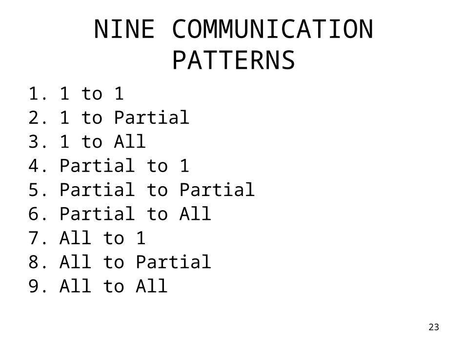
NINE COMMUNICATION PATTERNS

1. 1 to 1 2. 1 to Partial 3. 1 to All 4. Partial to 1 5. Partial to Partial6. Partial to All7. All to 18. All to Partial 9. All to All

24

Communication Patterns

SENDER

Figure 6: Nine Communication Patterns: (A) A single processor can send one message (same) to one processor, to a sub-group of M processors, or to the entire system. (B) A subgroup of M processors or all processors can send M different messages or all different messages to one processor.(C) A sub-group of K processors (how the messages are partitioned is a separate issue) can send messages to the entire system.

Finally, the entire system of P processors can send P different messages to one processor, a sub-group of N processors, or to the entire system.

Note: 1. In the obvious case of one message to 1, K, or P processors (same case in reverse), messages are partitioned naturally. 2. But in the case of M messages sent to K processors, the matter is a different problem and we will discuss that later.

RECEIVER

1 All

1 1

1 M

M 1 All 1

K P

All(P) All(P)

(A)

(B)

(C )

25

PARALLEL PROGRAMMING TOOLS

1. Parallel computing languages (parallel FORTRAN, C, C++ etc)

1.1 Message-passing assistant,

1.2 Portability helper: PVM, MPI......

2. Debuggers

3. Performance analyzer

4. Queuing system (same as in sequential)

26