Parallel Peeling Algorithms - DIMACSdimacs.rutgers.edu/Workshops/ParallelAlgorithms/Slides/F_justin_t... · The Peeling Paradigm ! Many important algorithms for a wide variety of

Justin Thaler, Yahoo Labs Joint Work with:

Michael Mitzenmacher, Harvard University Jiayang Jiang

Parallel Peeling Algorithms

The Peeling Paradigm �  Many important algorithms for a wide variety of problems can be

modeled in the same way. �  Start with a (random) hypergraph G.

�  While there exists a node v of degree less than k: �  Remove v and all incident edges.

�  The remaining graph is called the k-core of G. �  k=2 in most applications.

�  Typically, the algorithm “succeeds” if the the k-core is empty. �  To ensure “success”, data structure should be designed large enough

so that the k-core of G is empty w.h.p.

�  Typically yields simple, greedy algorithms running in linear time.

The peeling process when k=2





Example Algorithms

Example 1: Sparse Recovery Algorithms �  Consider data streams that insert and delete a lot of items.

�  Flows through a router, people entering/leaving a building. �  Sparse Recovery problem: list all items with non-zero frequency. �  Want listing not at all times, but at “reasonable” or “off-peak”

times, when working set size is bounded. �  If we do M insertions, then M-N deletions, and want a list at the end,

we need to list N items. �  Data structure size should be proportional to N, not to M!

�  Proportional to size you want to be able to list, not number of items your system has to handle.

�  Central primitive used in more complicated streaming algorithms. �  E.g. L0 sampling, which is in turn used to solve problems on dynamic

graph streams (see previous talk).

Example 1: Sparse Recovery Algorithms �  For simplicity, assume that when listing occurs, no item has

frequency more than 1.

Example 1: Sparse Recovery Algorithms �  Sparse Recovery Algorithm: Invertible Bloom Lookup Tables (IBLTs)

[Goodrich, Mitzenmacher]

Each stream item hashed to r cells (using r different hash functions)

Count KeySum

Insert(x): For each of the j cells that x is hashed to: Add key to KeySum Increment Count

Delete(x): For each of the j cells x is hashed to: Subtract key from keysum Decrement Count

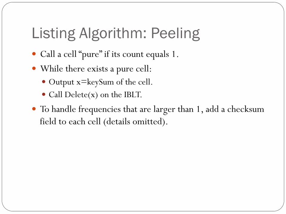
Listing Algorithm: Peeling �  Call a cell “pure” if its count equals 1. �  While there exists a pure cell:

� Output x=keySum of the cell. � Call Delete(x) on the IBLT.

To handle frequencies that are larger than 1, add a checksum field (details omitted). Listing peeling to 2-core on the hypergraph G where:

Cells vertices of G. Items in IBLT hyperedges of G. is r-uniform (each edge has r vertices).



�  To handle frequencies that are larger than 1, add a checksum field to each cell (details omitted).

Listing peeling to 2-core on the hypergraph G where: Cells vertices of G. Items in IBLT hyperedges of G. is r-uniform (each edge has r vertices).



�  To handle frequencies that are larger than 1, add a checksum field to each cell (details omitted).

�  Listing peeling to 2-core on the hypergraph G where: � Cells vertices of G. �  Items in IBLT hyperedges of G. � G is r-uniform (each edge has r vertices, one for each cell the item

is hashed to).

How Many Cells Does an IBLT Need to Guarantee Successful Listing?

�  Consider a random r-uniform hypergraph G with n nodes and m=c*n edges. �  i.e., each edge has r vertices, chosen uniformly at random from [n]

without repetition.

�  Known fact: Appearance of a non-empty k-core obeys a sharp threshold. �  For some constant ck,r, when m < ck,rn, the k-core is empty with

probability 1-o(1). � When m > ck,rn, the k-core of G is non-empty with probability 1-o(1). �  Implication: to successfully list a set of size M with probability 1-o(1),

the IBLT needs roughly M/ck,r cells.

�  E.g. c2,3≈0.818, c2,4≈0.772, c3,3≈1.553.

How Many Cells Does an IBLT Need to Guarantee Successful Listing?

�  Consider a random r-uniform hypergraph G with n nodes and m=c*n edges. �  i.e., each edge has r vertices, chosen uniformly at random from [n]

without repetition.

�  Known fact: Appearance of a non-empty k-core obeys a sharp threshold. �  For some constant ck,r, when m < ck,rn, the k-core is empty with

probability 1-o(1). � When m > ck,rn, the k-core of G is non-empty with probability 1-o(1). �  Implication: to successfully list a set of size M with probability 1-o(1),

the IBLT needs roughly M/ck,r cells.

�  E.g. c2,3≈0.818, c2,4≈0.772, c3,3≈1.553.

�  In general:

depends on the distance between the edge density and the threshold density c⇤k,r; we refer to this distance asn . Section 7 extends the analysis of Section 3 to precisely characterize this dependence, demonstrating thatthere is an additive Q(1/

pn) term in the number of rounds required. Section 8 concludes.

2 Preliminaries

For constants r � 2 and c, let Grn,cn denote a random hypergraph1 with n vertices and cn edges, where each

edge consists of r distinct vertices. Such hypergraphs are called r-uniform, and we refer to c as the edgedensity of Gr

n,cn. Previous analyses of random hypergraphs have determined the threshold values c⇤k,r suchthat when c < c⇤k,r, the k-core is empty with probability 1� o(1), and when c > c⇤k,r, the k-core is non-empty with probability 1�o(1). Here and throughout this paper, k,r � 2, but the special (and already wellunderstood) case of k = r = 2 is excluded from consideration. From [19], the formula for c⇤k,r is given by

c⇤k,r = minx>0

x

r(1� e�x Âk�2j=0

x j

j! )r�1

. (2.1)

For example, we find that c⇤2,3 ⇡ 0.818, c⇤2,4 ⇡ 0.772 and c⇤3,3 ⇡ 1.553.

3 Below the Threshold

In this section, we characterize the number of rounds required by the peeling process when the edge densityc is a constant strictly below the threshold density c⇤k,r. Recall that this peeling process repeatedly removesvertices with degree less than k, together with their incident edges. We prove the following theorem.

Theorem 1. Let k,r � 2 with k + r � 5, and let c be a constant. With probability 1� o(1), the parallelpeeling process for the k-core in a random hypergraph Gr

n,cn with edge density c and r-ary edges terminatesafter 1

log((k�1)(r�1)) log logn+O(1) rounds when c < c⇤k,r.

Theorem 1 is tight up to an additive constant.


n,cn with edge density c and r-ary edges requires1

log((k�1)(r�1)) log logn�O(1) rounds to terminate when c < c⇤k,r.

In proving Theorems 1 and 2, we begin in Section 3.1 with a high-level overview of our argument, beforepresenting full details of the proof in Section 3.2.

3.1 The High-Level Argument

The neighborhood of a node v in a random r-uniform hypergraph can be accurately modeled as a branchingprocess, with a random number of edges adjacent to this vertex, and similarly a random number of edgesadjacent to each of those vertices, and so on. For intuition, we assume this branching process yields a tree,and further that the number of adjacent edges is distributed according to a discrete Poisson distribution withmean rc. These assumptions are sufficiently accurate for our analysis, as we later prove. (This approach isstandard; see e.g. [6, 19] for similar arguments.)

1When r = 2 we have a graph, but we may use hypergraph when speaking generally.

3

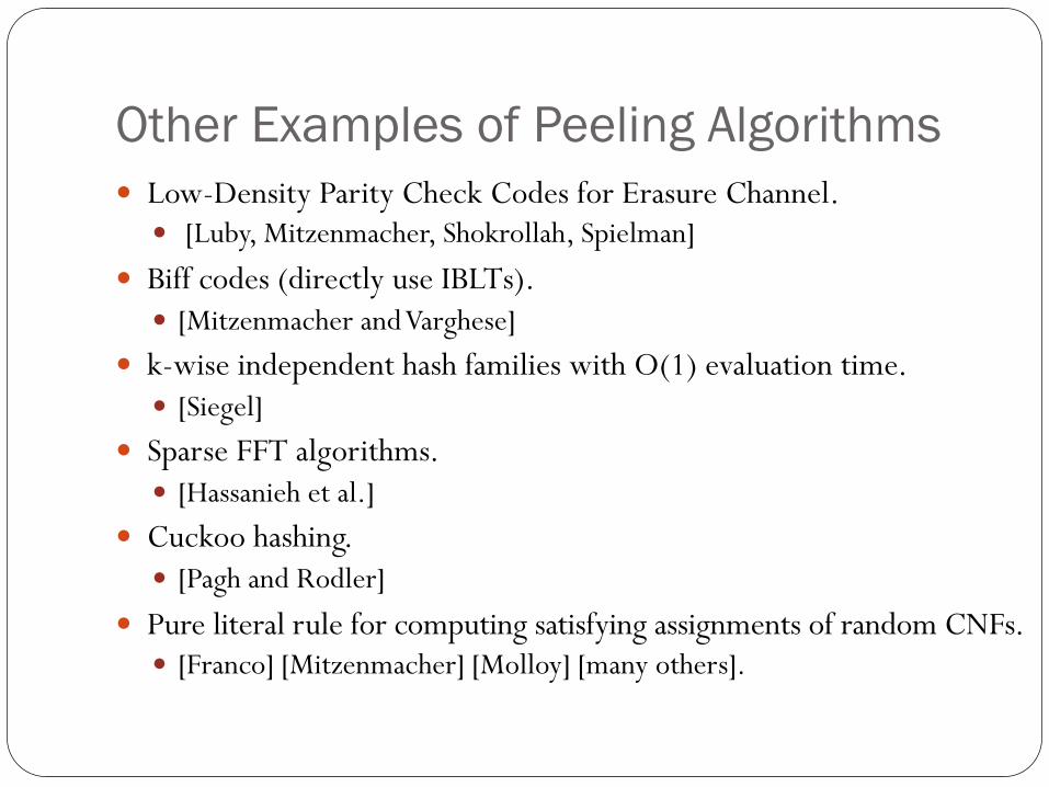
Other Examples of Peeling Algorithms �  Low-Density Parity Check Codes for Erasure Channel.

�  [Luby, Mitzenmacher, Shokrollah, Spielman] �  Biff codes (directly use IBLTs).

�  [Mitzenmacher and Varghese] �  k-wise independent hash families with O(1) evaluation time.

�  [Siegel] �  Sparse FFT algorithms.

�  [Hassanieh et al.] �  Cuckoo hashing.

�  [Pagh and Rodler] �  Pure literal rule for computing satisfying assignments of random CNFs.

�  [Franco] [Mitzenmacher] [Molloy] [many others].

Parallel Peeling Algorithms

Our Goal: Parallelize These Peeling Algorithms

�  Recall: the aforementioned algorithms are equivalent to peeling a random hypergraph G to its k-core.

�  There is a brain dead way to parallelize the peeling process. �  For each node v in parallel:

�  Check if v has degree less than k. �  If so, remove v and its incident hyperedges.

�  Key question: how many rounds of peeling are required to find the k-core?

�  Algorithm is simple, analysis is tricky.

Main Result �  Two behaviors:

�  Parallel peeling completes in O(log log n) rounds if the edge density c is “below the threshold” ck,r.

�  Parallel peeling requires Ω(log n) rounds if the edge density c is “above the threshold” ck,r .

�  This is great! � Most peeling uses the goal is to be below the threshold. �  So “nature” is helping us by making parallelization fast. �  Implies poly(loglog n) time, O(n poly(loglog n)) work, parallel

algorithms for listing elements in an IBLT, decoding LDPC codes, etc.

Precise Upper Bound

Summary: The right factor in front of the loglog n is 1/(log(k-1)(r-1)) (tight up to an additive constant).



2 Preliminaries




c⇤k,r = minx>0

x

r(1� e�x Âk�2j=0

x j

j! )r�1

. (2.1)















3



2 Preliminaries




c⇤k,r = minx>0

x

r(1� e�x Âk�2j=0

x j

j! )r�1

. (2.1)















3

Lower Bound

Summary: Ω(log n) lower bound matches an earlier O(log n) upper bound due to [Achlioptas and Molloy, 2013].

of Lt by only logc2(n), so Azuma’s martingale inequality2 [16, Theorem 12.4] yields for sufficiently large n:

Pr(|Lt �E[Lt ]|� n1/2 logc2+1(n)) 2e�n log2c2+2(n)/(2m log2c2 (n))

e� log3/2(n) 1/n.

In particular, this means that with probability 1�o(1) there remain unpeeled vertices in Grc after t rounds of

peeling.

4 Above the Threshold

We now consider the case when c > c⇤k,r. We show that parallel peeling requires W(logn) rounds in this case.Molloy [19] showed that in this case there exists a r > 0 such that limt!• rt = r . Similarly, limt!• bt =

b > 0 and limt!• lt = l > 0. It follows that the core will have size ln+o(n). We examine how bt and lt

approach their limiting values to show that the parallel peeling algorithm takes W(logn) rounds.

Theorem 3. Let r � 3 and k � 2. With probability 1� o(1), the peeling process for the k-core in Grn,cn

terminates after W(logn) rounds when c > c⇤k,r,

Proof. First, note that b corresponds to the fixed point

b =

1� e�b

k�2

Âj=0

b j

j!

�r�1

rc. (4.1)

Let bi = b + di, where di > 0. We begin by working in the idealized branching process model given inSection 3.1 to determine the behavior of bi. Starting with Equation (3.4) and considering bi+1 as a functionof di, we obtain:

bi+1 =

1� e�b�di

k�2

Âj=0

(b +di) j

j!

�r�1

rc. (4.2)

We now view the right hand side of Equation (4.2) as a function of di. Denoting this function as f (di),we take a Taylor series expansion around 0 and conclude that:

f (di) = f (0)+ f 0(0)di +Q( f 00(0)d 2i ).

Equation (4.1) immediately implies that f (0) = b . Moreover, it can be calculated that

f 0(0) =(r�1)be�b

1� e�b Âk�2j=0

b j

j!

b k�2

(k�2)!(4.3)

In particular, it holds that0 < f 0(0)< 1. (4.4)

Note that while f 0(0) < 1 can be checked explicitly, this condition also follows immediately from theconvergence of the bi values to b .

2Formally, to cope with conditioning on events E1 and E2 in the application of Azuma’s inequality, we must actually consider aslightly modified martingale. This technique is standard, and the details can be found in Section 4.

12

Proof Sketch for Upper Bound •  Let denote the probability a given vertex v survives rounds of peeling. •  Claim: •  Suggests after about rounds. •  A related argument shows that

and after that point the claim implies that falls doubly-exponentially quickly.

iλi+1 ≤ (Cλi )

(k−1)(r−1) for some constant C.λi <<1/ n 1/ ((k −1)(r −1))* loglogn

λi ≤1/ (2C) after O(1) rounds,λi

λi

Proof Sketch for Upper Bound •  Let denote the probability a given vertex v survives rounds of peeling. •  Claim: •  Very crude sketch of the Claim’s plausibility: •  Node survives round i+1 only if it has (at least) k incident edges

that survive round •  Fix a k-tuple of edges incident to v. •  Assume no node other than v appears in more than one of these edges. •  Then there are k(r-1) distinct nodes other than v appearing in these edges. •  The edges all survive round i only if all k(r-1) of these nodes survive round i. •  Let’s pretend that the survival of these nodes are independent events. •  Then the probability all nodes survive round i is roughly •  Finally, union bound over all k-tuples of edges incident to v.

vi.e1...ek

e1...ek

λik (r−1).

iλi+1 ≤ (Cλi )

(k−1)(r−1) for some constant C.λi

Simulation Results

•  Results from simulations of parallel peeling process on random 4-uniform hypergraphs with n nodes and c*n edges using k = 2.

•  Averaged over 1000 trials. •  Recall that c2,4≈0.772.

Refined Result: Mind the Gap

Summary: below the threshold, the additive term is Θ(1/√|gap|). This can be more important than the log log n term if the edge

density is close to the threshold!

Refined Simulations: Mind the Gap

Plots show expected progress of the peeling process as a function of the round i, for values of the edge density c approaching the threshold value of

c2,4≈0.772.

Refined Analysis: Mind the Gap •  Analysis shows that peeling process falls into three “stages”. •  First stage: the fraction of surviving nodes falls very quickly

as a function of the rounds until it gets close to a certain key value x*.

•  Second stage: Θ(1/√|gap|) rounds are required to go from “close” to x* to “significantly below” x*.

•  Third stage: the analysis of the basic upper bound kicks in, and the fraction of surviving nodes falls doubly-exponentially quickly.

Implementation Issues

GPU Experimental Results

Table No. Table % GPU Serial GPU SerialLoad Cells Recovered Recovery Time Recovery Time Insert Time Insert Time0.75 16.8 million 100% 0.33 s 6.37 s 0.31 s 3.91 s0.83 16.8 million 50.1% 0.42 s 3.64 s 0.35 s 4.34 s

Table 3: Results of our parallel and serial IBLT implementations with r = 3 hash functions. The table loadrefers to the ratio of the number of items in the IBLT to the number of cells in the IBLT.

Table No. Table % GPU Serial GPU SerialLoad Cells Recovered Recovery Time Recovery Time Insert Time Insert Time0.75 16.8 million 100% 0.47 s 8.37 s 0.42 s 4.55 s0.83 16.8 million 24.6% 0.25 s 2.28 s 0.46 s 5.0 s

Table 4: Results of our parallel and serial IBLT implementations with r = 4 hash functions. The table loadrefers to the ratio of the number of items in the IBLT to the number of cells in the IBLT.

Summary of results. Relative to our serial implementation, our GPU implementation achieves 10x-12xspeedups for theinsertion/deletion phase, and 20x speedups for the recovery stage when the edge density of the hypergraphis below the threshold for successful recovery (i.e. empty 2-core). When the edge density is slightly abovethe threshold for successful recovery, our parallel recovery implementation was only about 7x faster thanour serial implementation. The reasons for this are two-fold. Firstly, above the threshold, many more roundsof the parallel peeling process were necessary before the 2-core was found. Secondly, above the threshold,less work was required of the serial implementation because fewer items were recovered; in contrast, theparallel implementation examines every cell in every round.

Our detailed experimental results are given in Tables 3 (for the case of r = 3 hash functions) and 4(for the case of r = 4 hash functions). The timing results are averages over 10 trials each. For the GPUimplementation, the reported times do count for the time to transfer data (i.e. the items to be inserted) fromthe CPU to the GPU.

The reported results are for a fixed IBLT size, consisting of 224 cells. These results are representativefor all sufficiently large input sizes: once the number of IBLT cells is larger than about 219, the runtime ofour parallel implementation grows roughly linearly with the number of table cells (for any fixed table load).Here, table load refers to the ratio of the number of items in the IBLT to the number of cells in the IBLT. Thiscorresponds to the edge density c in the corresponding hypergraph. The linear increase in runtime above acertain input size is typical, and is due to the fact that there is a finite number of threads that the GPU canlaunch at any one time.

7 Rounds as a Function of the Distance from the Threshold

Recall that the hidden constant in the O(1) term of Theorem 1 depends on the size of the “gap” n = c⇤k,r � cbetween the edge density and the threshold density. This term can be significant in practice when n is small,and in this section, we make the dependence on n explicit. Specifically, we extend the analysis of Section3 to characterize how the growth of the number of rounds depends on c⇤k,r � c, when c is a constant withc < c⇤k,r. The proof of Theorem 5 below is in Appendix C.

Theorem 5. Let n = |c⇤k,r�c| for constant c with c< ck,r. With probability 1�o(1), peeling in Grn,cn requires

Q(p

1/n)+ 1log((k�1)(r�1)) log logn rounds when c is below the threshold density c⇤k,r.

17

Recall: IBLTs

Each stream item hashed to r cells (using r different hash functions)

Count KeySum

Insert(x): For each of the j cells that x is hashed to: Add key to KeySum Increment Count

Delete(x): For each of the j cells x is hashed to: Subtract key from keysum Decrement Count

Recall: IBLT Listing Algorithm �  Call a cell “pure” if its count equals 1. �  While there exists a pure cell:


To handle frequencies that are larger than 1, add a checksum field (details omitted). Listing peeling to 2-core on the hypergraph G where:

Cells vertices of G. Items in IBLT hyperedges of G. is r-uniform (each edge has r vertices).

GPU Implementation �  Each cell gets a thread. �  Each cell checks if it is pure.

�  If so, identify the key it contains and remove it from other cells in the IBLT.

� Do this by subtracting out values in other cells.

�  Issue: repeated deletion. �  Several cells might recover and try to remove the same key in

the same round. So a key gets deleted more than once!

Dealing with Repeated Deletion �  To avoid this: use r subtables, such that the ith hash function only

hashes into subtable i. �  Break the listing algorithm into serial subrounds. In ith subround,

recover only from the ith subtable. �  Avoids repeated deletions, since each item will be hashed to just 1 cell

in each subtable. �  Leads to interesting variation in the analysis.

�  Subrounds increase runtime, since they must happen sequentially. �  Naively, they may blow up runtime by a factor of r. �  But we show this does not happen.

�  Gains in one subround can help later subrounds. �  We show runtime only blows up by a factor of about log2(r-1).

�  Analysis is similar to Vöcking’s d-left scheme. �  Fibonacci numbers show up!

Subround Result

Summary: use of r subtables increase constant factor in front of the log log n, but by much less than a factor or r.

Conclusion �  Peeling gives simple, fast greedy algorithms.

� Usually linear or quasi-linear total work.

�  Particularly well suited for parallelization. �  Especially when aiming for an empty k-core.

�  Implementation leads to interesting variation in the analysis. �  Subrounds.

�  Can analyze dependence on “gap” to the threshold.

Thank you!

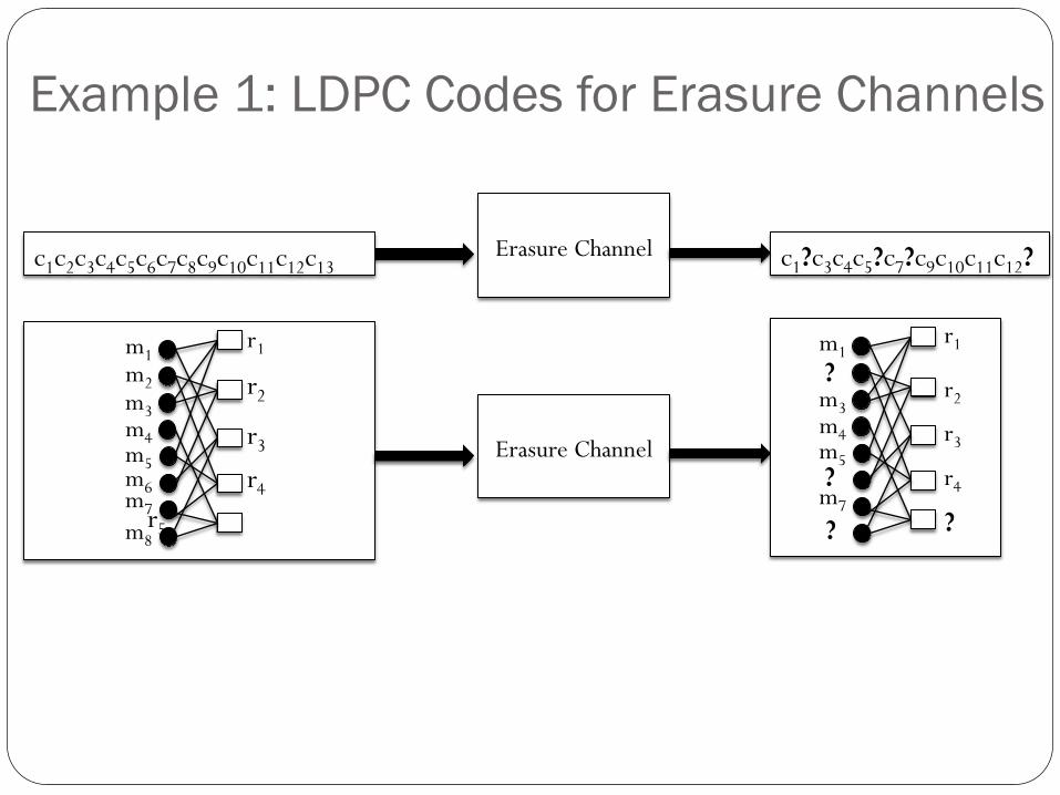
Example 1: LDPC Codes for Erasure Channels

Erasure Channel c1c2c3c4c5c6c7c8c9c10c11c12c13 c1?c3c4c5?c7?c9c10c11c12?



How does an LDPC code encode an 8-bit message m1m2m3m4m5m6m7m8?



How does an LDPC code encode an 8-bit message m1m2m3m4m5m6m7m8?

m1 m2 m3 m4 m5 m6 m7 m8

r1=XOR(m1, m3, m5)

r2=XOR(m2, m3, m6) r3=XOR(m1, m6, m8) r4=XOR(m2, m5, m7) r5=XOR(m4, m7, m8)



m1 m2 m3 m4 m5 m6 m7 m8

r1

r2

Erasure Channel

m1 ? m3 m4 m5 ? m7

?

r1

r2

r3

r4

?

r3 r4 r5



m1 m2 m3 m4 m5 m6 m7 m8

r1

r2

Erasure Channel

m1 ? m3 m4 m5 ? m7

?

r1

r2

r3

r4

?

r3 r4 r5

Decoding Algorithm: While there exists an un-erased a parity-check bit with exactly one un-erased neighbor:

Recover the neighbor



m1 m2 m3 m4 m5 m6 m7 m8

r1

r2

Erasure Channel

m1 ? m3 m4 m5 ? m7

?

r1

r2

r3

r4

?

r3 r4 r5





m1 m2 m3 m4 m5 m6 m7 m8

r1

r2

Erasure Channel

m1

m3 m4 m5 ? m7

?

r1

r2

r3

r4

?

r3 r4 r5



m2



m1 m2 m3 m4 m5 m6 m7 m8

r1

r2

Erasure Channel

m1

m3 m4 m5 ? m7

?

r1

r2

r3

r4

?

r3 r4 r5



m2



m1 m2 m3 m4 m5 m6 m7 m8

r1

r2

Erasure Channel

m1

m3 m4 m5

m7

?

r1

r2

r3

r4

?

r3 r4 r5



m2

m6



m1 m2 m3 m4 m5 m6 m7 m8

r1

r2

Erasure Channel

m1

m3 m4 m5

m7

?

r1

r2

r3

r4

?

r3 r4 r5



m2

m6



m1 m2 m3 m4 m5 m6 m7 m8

r1

r2

Erasure Channel

m1

m3 m4 m5

m7

r1

r2

r3

r4

?

r3 r4 r5



m2

m6

m8



m1 m2 m3 m4 m5 m6 m7 m8

r1

r2

Erasure Channel

m1

m3 m4 m5

m7

r1

r2

r3

r4

?

r3 r4 r5

•  Decoding peeling to 2-core on the hypergraph G where: •  Parity-check bits vertices of G, •  Erased message bits hyperedges of G.

•  Yields capacity-achieving codes with linear encoding and decoding time [Luby, Mitzenmacher, Shokrollahi, Spielman]

m2

m6

m8

Documents

Parallel Peeling Algorithms - DIMACSdimacs.rutgers.edu/Workshops/ParallelAlgorithms/Slides/F_justin_t... · The Peeling Paradigm ! Many important algorithms for a wide variety of