Embed Size (px)
Citation preview

JOURNAL OF PARALLEL AND DISTRIBUTED COMPUTING48, 71–95 (1998)ARTICLE NO. PC971403
A Parallel Algorithm for Multilevel GraphPartitioning and Sparse Matrix Ordering1
George Karypis2 and Vipin Kumar3
Department of Computer Science/Army HPC Research Center, University
of Minnesota, Minneapolis, Minnesota 55455
In this paper we present a parallel formulation of the multilevel graphpartitioning and sparse matrix ordering algorithm. A key feature of our parallelformulation (that distinguishes it from other proposed parallel formulations ofmultilevel algorithms) is that it partitions the vertices of the graph into
√p parts
while distributing the overall adjacency matrix of the graph among allp processors.This mapping results in substantially smaller communication than one-dimensionaldistribution for graphs with relatively high degree, especially if the graph israndomly distributed among the processors. We also present a parallel algorithmfor computing a minimal cover of a bipartite graph which is a key operation forobtaining a small vertex separator that is useful for computing the fill reducingordering of sparse matrices. Our parallel algorithm achieves a speedup of up to56 on 128 processors for moderate size problems, further reducing the alreadymoderate serial run time of multilevel schemes. Furthermore, the quality of theproduced partitions and orderings are comparable to those produced by the serialmultilevel algorithm that has been shown to outperform both spectral partitioningand multiple minimum degree.© 1998 Academic Press
Key Words:parallel graph partitioning; multilevel partitioning methods; fillreducing ordering; numerical linear algebra.
1This work was supported by NSF CCR-9423082, by the Army Research Office Contract DA/DAAH04-95-1-0538, by the IBM Partnership Award, and by Army High Performance Computing Research Center under theauspices of the Department of the Army, Army Research Laboratory Cooperative Agreement Number DAAH04-95-2-0003/Contract DAAH04-95-C-0008, the content of which does not necessarily reflect the position or thepolicy of the government, and no official endorsement should be inferred. Access to computing facilitieswas provided by AHPCRC. Minnesota Supercomputer Institute, Cray Research Inc., and by the PittsburghSupercomputing Center. Related papers are available via WWW at URL: http://www.cs.umn.edu/∼karypis.
2E-mail: [email protected]: [email protected].
71
0743-7315/98 $25.00Copyright © 1998 by Academic Press
All rights of reproduction in any form reserved.

72 KARYPIS AND KUMAR
1. INTRODUCTION
Graph partitioning is an important problem that has extensive applications in manyareas, including scientific computing, VLSI design, task scheduling, geographicalinformation systems, and operations research. The problem is to partition the verticesof a graph top roughly equal parts, such that the number of edges connecting verticesin different parts is minimized. For example, the solution of a sparse system of linearequationsAx = b via iterative methods on a parallel computer gives rise to a graphpartitioning problem. A key step in each iteration of these methods is the multiplication ofa sparse matrix and a (dense) vector. Partitioning the graph that corresponds to matrixA isused to significantly reduce the amount of communication [19]. If parallel direct methodsare used to solve a sparse system of equations, then a graph partitioning algorithm canbe used to compute a fill reducing ordering that lead to high degree of concurrencyin the factorization phase [8, 19]. The multiple minimum degree ordering used almostexclusively in serial direct methods is not suitable for parallel direct methods, as itprovides limited concurrency in the parallel factorization phase.
The graph partitioning problem is NP-complete. However, many algorithms have beendeveloped that find a reasonably good partition. Recently, a new class of multilevel graphpartitioning techniques was introduced by Bui and Jones [4] and Hendrickson and Leland[12], and further studied by Karypis and Kumar [13, 15, 16]. These multilevel schemesprovide excellent graph partitionings and have moderate computational complexity. Eventhough these multilevel algorithms are quite fast compared with spectral methods, parallelformulations of multilevel partitioning algorithms are needed for the following reasons.The amount of memory on serial computers is not enough to allow the partitioning ofgraphs corresponding to large problems that can now be solved on massively parallelcomputers and workstation clusters. A parallel graph partitioning algorithm can takeadvantage of the significantly higher amount of memory available in parallel computers.Furthermore, with recent development of highly parallel formulations of sparse Choleskyfactorization algorithms [9, 17, 25], numeric factorization on parallel computers can takemuch less time than the step for computing a fill-reducing ordering on a serial computer.For example, on a 1024-processor Cray T3D, some matrices can be factored in a fewseconds using our parallel sparse Cholesky factorization algorithm [17], but serial graphpartitioning (required for ordering) takes several minutes for these problems.
In this paper we present a parallel formulation of the multilevel graph partitioningand sparse matrix ordering algorithm. A key feature of our parallel formulation (thatdistinguishes it from other proposed parallel formulations of multilevel algorithms [1, 2,14, 24]) is that it partitions the vertices of the graph into
√p parts while distributing the
overall adjacency matrix of the graph among allp processors. This mapping resultsin substantially smaller communication than one-dimensional distribution for graphswith relatively high degree, especially if the graph is randomly distributed among theprocessors. We also present a parallel algorithm for computing a minimal cover of abipartite graph which is a key operation for obtaining a small vertex separator that isuseful for computing the fill reducing ordering of sparse matrices. Our parallel algorithmachieves a speedup of up to 56 on 128 processors for moderate size problems, furtherreducing the already moderate serial run time of multilevel schemes. Furthermore, thequality of the produced partitions and orderings are comparable to those produced by theserial multilevel algorithm that has been shown to outperform both spectral partitioning

PARALLEL ALGORITHM FOR GRAPH PARTITIONING 73
and multiple minimum degree [16]. The parallel formulation in this paper is describedin the context of the serial multilevel graph partitioning algorithm presented in [16].However, nearly all of the discussion in this paper is applicable to other multilevel graphpartitioning algorithms [4, 7, 12, 22].
The rest of the paper is organized as follows. Section 2 surveys the different typesof graph partitioning algorithms that are widely used today and briefly describes theserial multilevel algorithm that forms the basis for the parallel algorithm described inSections 3 and 4 for graph partitioning and sparse matrix ordering, respectively. Section5 analyzes the complexity and scalability of the parallel algorithm. Section 6 presents theexperimental evaluation of the parallel multilevel graph partitioning and sparse matrixordering algorithm. Section 7 provides some concluding remarks.
2. THE GRAPH PARTITIONING PROBLEM AND MULTILEVELGRAPH PARTITIONING
The p-way graph partitioning problem is defined as follows: Given a graphG = (V,E) with |V| = n, partitionV into p subsets,V1, V2, . . . , Vp such thatVi ∩ Vj = ∅ for i ≠ j,|Vi| = n/p, and
⋃i Vi = V, and the number of edges ofE whose incident vertices belong
to different subsets is minimized. Ap-way partitioning ofV is commonly represented bya partitioning vectorP of lengthn, such that for every vertexv ∈ V, P[v] is an integerbetween 1 andp, indicating the partition to which vertexv belongs. Given a partitioningP, the number of edges whose incident vertices belong to different partitions is calledthe edge-cutof the partition.
The p-way partitioning problem is most frequently solved by recursive bisection. Thatis, we first obtain a 2-way partition ofV, and then we further subdivide each part using 2-way partitions. After logp phases, graphG is partitioned intop parts. Thus, the problemof performing ap-way partition is reduced to that of performing a sequence of 2-waypartitions or bisections. Even though this scheme does not necessarily led to optimalpartition [15, 27], it is used extensively due to its simplicity [8, 10].
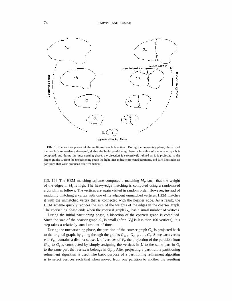
The basic structure of the multilevel bisection algorithm is very simple. The graphG =(V, E) is first coarsened down to a few thousand vertices (coarsening phase), a bisection ofthis much smaller graph is computed (initial partitioning phase), and then this partition isprojected back towards the original graph (uncoarsening phase), by periodically refiningthe partition [4, 12, 16]. Since the finger graph has more degrees of freedom, suchrefinements improve the quality of the partitions. This process, is graphically illustratedin Fig. 1.
During the coarsening phase, a sequence of smaller graphsGl = (Vl, El) is constructedfrom the original graphG0 = (V0, E0) such that |Vl| > |Vl+1|. GraphGl+1 is constructedfrom Gl by finding a maximal matchingMl ⊆ El of Gl and collapsing together the verticesthat are incident on each edge of the matching. Maximal matchings can be computed indifferent ways [4, 12, 15, 16]. The method used to compute the matching greatly affectsboth the quality of the partitioning, and the time required during the uncoarsening phase.One simple scheme for computing a matching is therandom matching(RM) scheme [4,12]. In this scheme, vertices are visited in random order, and for each unmatched vertexwe randomly match it with one of its unmatched neighbors. An alternative matchingscheme that we have found to be quite effective is calledheavy-edge matching(HEM)
74 KARYPIS AND KUMAR
FIG. 1. The various phases of the multilevel graph bisection. During the coarsening phase, the size ofthe graph is successively decreased; during the initial partitioning phase, a bisection of the smaller graph iscomputed, and during the uncoarsening phase, the bisection is successively refined as it is projected to thelarger graphs. During the uncoarsening phase the light lines indicate projected partitions, and dark lines indicatepartitions that were produced after refinement.
[13, 16]. The HEM matching scheme computes a matchingMl, such that the weightof the edges inMl is high. The heavy-edge matching is computed using a randomizedalgorithm as follows. The vertices are again visited in random order. However, instead ofrandomly matching a vertex with one of its adjacent unmatched vertices, HEM matchesit with the unmatched vertex that is connected with the heavier edge. As a result, theHEM scheme quickly reduces the sum of the weights of the edges in the coarser graph.The coarsening phase ends when the coarsest graphGm has a small number of vertices.
During the initial partitioning phase, a bisection of the coarsest graph is computed.Since the size of the coarser graphGk is small (often |Vk| is less than 100 vertices), thisstep takes a relatively small amount of time.
During the uncoarsening phase, the partition of the coarser graphGm is projected backto the original graph, by going through the graphsGm−1, Gm−2, . . . , G1. Since each vertexu ∈ Vl+1 contains a distinct subsetU of vertices ofVl, the projection of the partition fromGl+1 to Gl is constructed by simply assigning the vertices inU to the same part inGl
to the same part that vertexu belongs inGl+1. After projecting a partition, a partitioningrefinement algorithm is used. The basic purpose of a partitioning refinement algorithmis to select vertices such that when moved from one partition to another the resulting

PARALLEL ALGORITHM FOR GRAPH PARTITIONING 75
partitioning has smaller edge-cut and remains balanced (i.e., each part has the sameweight). A class of local refinement algorithms that tend to produce very good resultsare those that are based on the Kernighan–Lin (KL) partitioning algorithm [18] and theirvariants (FM) [6, 12, 16].
3. PARALLEL MULTILEVEL GRAPHPARTITIONING ALGORITHM
There are two types of parallelism that can be exploited in thep-way graph partitioningalgorithm based on the multilevel bisection described in Section 2. The first type ofparallelism is due to the recursive nature of the algorithm. Initially, a single processorfinds a bisection of the original graph. Then, two processors find bisections of the twosubgraphs just created and so on. However, this scheme by itself can use only up tolog p processors, and reduces the overall run time of the algorithm only by a factor ofO(log p). We will refer to this type of parallelism as the parallelism associated with therecursive step.
The second type of parallelism that can be exploited is during thebisection step. In thiscase, instead of performing the bisection of the graph on a single processor, we perform itin parallel. We will refer to this type of parallelism as the parallelism associated with thebisection step. Note that if the bisection step is parallelized, then the speedup obtainedby the parallel graph partitioning algorithm can be significantly higher thanO(log p).
The parallel graph partitioning algorithm we describe in this section exploits both ofthese types of parallelism. Initially all the processors cooperate to bisect the originalgraphG into G0 andG1. Then, half of the processors bisectG0, while the other half ofthe processors bisectG1. This step creates four subgraphsG00, G01, G10, andG11. Theneach quarter of the processors bisect one of these subgraphs and so on. After logp steps,the graphG has been partitioned intop parts.
In the next three sections we describe how we have parallelized the three phases ofthe multilevel bisection algorithm.
3.1. Coarsening Phase
As described in Section 2, during the coarsening phase, a sequence of coarser graphsis constructed. A coarser graphGl+1 = (Vl+1, El+1) is constructed from the finer graphGl
= (Vl, El) by finding a maximal matchingMl and contracting the vertices and edges ofGl to form Gl+1. This is the most time consuming phase of the three phases; hence, itneeds to be parallelized effectively. Furthermore, the amount of communication requiredduring the contraction ofGl to form Gl+1 depends on how the matching is computed.
The randomized algorithms described in Section 2 for computing a maximal matchingon a serial computer are simple and efficient. However, computing a maximal matchingin parallel is difficult, particularly on a distributed memory parallel computer. A directparallelization of the serial randomized algorithms or algorithms based on depth-firstgraph traversals requires significant amount of communication. For instance, consider thefollowing parallel implementation of the randomized algorithms. Each processor containsa (random) subset of the graph. For each local vertexv, processors select an edge (v,u) to be in the matching. Now, the decision of whether or not an edge (v, u) canbe included in the matching may result in communication between the processors that

76 KARYPIS AND KUMAR
store v and u, to determine if vertexu has been matched or not. In addition to that,care must be taken to avoid race conditions, since vertexu may be checked due toanother edge (w, u), and only one of the edges (v, u) and (w, u) must be included in thematching. Similar problems arise when trying to parallelize algorithms based on depth-first traversal of the graph. Another possibility is to adapt some of the algorithms thathave been developed for the PRAM model. In particular, the algorithm of Luby [21] forcomputing the maximal independent set can be used to find a matching. However, parallelformulations of this type of algorithms also have high communication overhead becauseeach processorpi needs to communicate with all other processors that contain neighborsof the nodes local atpi. Furthermore, having computedMl using any one of the abovealgorithms, the construction of the next level coarser graph,Gl+1 requires significantamount of communication. This is because each edge ofMl may connect vertices whoseadjacent lists are stored on different processors, and during the contraction at least one ofthese adjacency lists needs to be moved from one processor to another. Communicationoverhead in any of the above algorithms can become small if the graph is initiallypartitioned among processors in such a way so that the number of edges going acrossprocessor boundaries are small. But this requires solving thep-way graph partitioningproblem that we are trying to solve using these algorithms.
Another way of computing a maximal matching is to divide then vertices amongpprocessors and then compute matchings between the vertices locally assigned to eachprocessor. The advantages of this approach is that no communication is required tocompute the matching, and since each pair of vertices that gets matched belongs tothe same processor, no communication is required to move adjacency lists betweenprocessors. However, this approach causes problems because each processor has veryfew nodes to match from. Also, even though there is no need to exchange adjacencylists among processors, each processor needs to know matching information about all thevertices that its local vertices are connected to in order to properly form the contractedgraph. As a result, a significant amount of communication is required. In fact, thiscomputation is very similar in nature to the multiplication of a randomly sparse matrix(corresponding to the graph) with a vector (corresponding to the matching vector).
In our parallel coarsening algorithm, we retain the advantages of the local matchingscheme, but minimize its drawbacks by computing the matchings between groups ofn/√
p vertices. This increases the size of the computed matchings and also reducesthe communication overhead for constructing the coarse graph. Specifically, our parallelcoarsening algorithm treats thep processors as a two-dimensional array of
√p × √p
processors (assume thatp = 22r). The vertices of the graphG0 = (V0, E0) are distributedamong this processor grid using a cyclic mapping [19]. The verticesV0 are partitionedinto√
p subsets,V00 , V1
0 , . . . , V√
p−10 . ProcessorPi, j stores the edges ofE0 between the
subsets of verticesVi0 and V j
0 . Having distributed the data in this fashion, the algorithmthen proceeds to find a matching. This matching is computed by the processors alongthe diagonal of the processor grid. In particular, each processorPi, i finds a heavy-edgematchingMi
0 using the set of edges it stores locally. The union of these√
p matchings istaken as the overall matchingM0. Since the vertices are split into
√p parts, this scheme
finds larger matchings than the one that partitions vertices intop parts.In order for the next level coarser graphG1 to be created, processorPi, j needs to know
the parts of the matching that were found by processorsPi, i and Pj, j (i.e., Mi0 and M j
0 ,
PARALLEL ALGORITHM FOR GRAPH PARTITIONING 77
respectively). Once it has this information, then it can proceed to create the edges ofG1
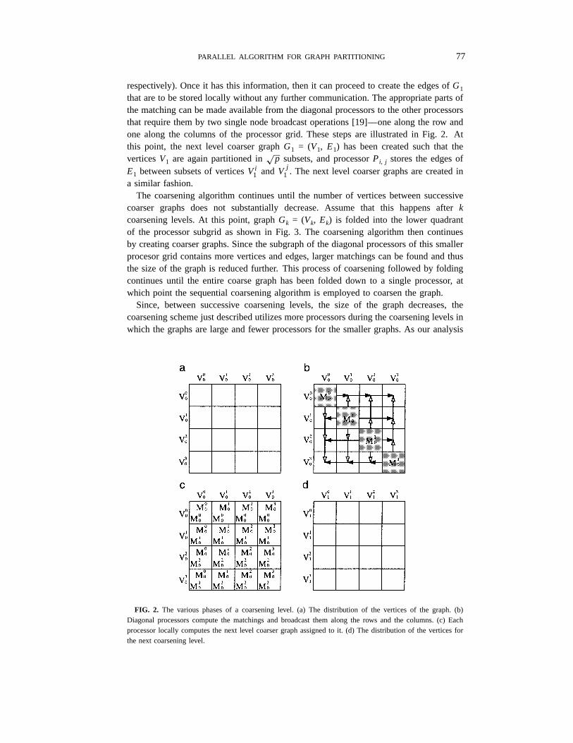
that are to be stored locally without any further communication. The appropriate parts ofthe matching can be made available from the diagonal processors to the other processorsthat require them by two single node broadcast operations [19]—one along the row andone along the columns of the processor grid. These steps are illustrated in Fig. 2. Atthis point, the next level coarser graphG1 = (V1, E1) has been created such that theverticesV1 are again partitioned in
√p subsets, and processorPi, j stores the edges of
E1 between subsets of verticesVi1 and V j
1 . The next level coarser graphs are created ina similar fashion.
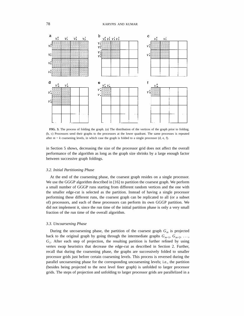
The coarsening algorithm continues until the number of vertices between successivecoarser graphs does not substantially decrease. Assume that this happens afterkcoarsening levels. At this point, graphGk = (Vk, Ek) is folded into the lower quadrantof the processor subgrid as shown in Fig. 3. The coarsening algorithm then continuesby creating coarser graphs. Since the subgraph of the diagonal processors of this smallerprocesor grid contains more vertices and edges, larger matchings can be found and thusthe size of the graph is reduced further. This process of coarsening followed by foldingcontinues until the entire coarse graph has been folded down to a single processor, atwhich point the sequential coarsening algorithm is employed to coarsen the graph.
Since, between successive coarsening levels, the size of the graph decreases, thecoarsening scheme just described utilizes more processors during the coarsening levels inwhich the graphs are large and fewer processors for the smaller graphs. As our analysis
FIG. 2. The various phases of a coarsening level. (a) The distribution of the vertices of the graph. (b)Diagonal processors compute the matchings and broadcast them along the rows and the columns. (c) Eachprocessor locally computes the next level coarser graph assigned to it. (d) The distribution of the vertices forthe next coarsening level.
78 KARYPIS AND KUMAR
FIG. 3. The process of folding the graph. (a) The distribution of the vertices of the graph prior to folding.(b, c) Processors send their graphs to the processors at the lower quadrant. The same processes is repeatedafter m − k coarsening levels, in which case the graph is folded to a single processor (d, e, f).
in Section 5 shows, decreasing the size of the processor grid does not affect the overallperformance of the algorithm as long as the graph size shrinks by a large enough factorbetween successive graph foldings.
3.2. Initial Partitioning Phase
At the end of the coarsening phase, the coarsest graph resides on a single processor.We use the GGGP algorithm described in [16] to partition the coarsest graph. We performa small number of GGGP runs starting from different random vertices and the one withthe smaller edge-cut is selected as the partition. Instead of having a single processorperforming these different runs, the coarsest graph can be replicated to all (or a subsetof) processors, and each of these processors can perform its own GGGP partition. Wedid not implement it, since the run time of the initial partition phase is only a very smallfraction of the run time of the overall algorithm.
3.3. Uncoarsening Phase
During the uncoarsening phase, the partition of the coarsest graphGm is projectedback to the original graph by going through the intermediate graphsGm−1, Gm−2, . . . ,G1. After each step of projection, the resulting partition is further refined by usingvertex swap heuristics that decrease the edge-cut as described in Section 2. Further,recall that during the coarsening phase, the graphs are successively folded to smallerprocessor grids just before certain coarsening levels. This process is reversed during theparallel uncoarsening phase for the corresponding uncoarsening levels; i.e., the partition(besides being projected to the next level finer graph) is unfolded to larger processorgrids. The steps of projection and unfolding to larger processor grids are parallelized in a
PARALLEL ALGORITHM FOR GRAPH PARTITIONING 79
way similar to their counterparts in the coarsening phase. Here we describe our parallelimplementation of the refinement step.
For refining the coarser graphs that reside on a single processor, we use the BoundaryKernighan–Lin refinement algorithm (BKLR) described in [16]. The BKLR algorithmis sequential in nature and it cannot be used in its current form to efficiently refine apartition when the graph is distributed among a grid of processors. In this case, we use adifferent algorithm that tries to approximate the BKLR algorithm but is more amenable toparallel computations. The key idea behind our parallel refinement algorithm is to selecta group of vertices to swap from one part to the other instead of selecting a single vertex.Refinement schemes that use similar ideas are described in [5, 26]; however, our algorithmdiffers in two important ways from the other schemes: (i) it uses a different method forselecting vertices; (ii) it uses a two-dimensional partition to minimize communication.
Consider a√
p × √p processor grid on which graphG = (V, E) is distributed.Furthermore, each processorPi, j computes the gain in the edge-cut obtained from movingvertexv ∈ Vj, to the other part by considering only the part ofG (i.e., vertices and edgesof G) stored locally atPi, j. This locally computed gain is calledlgv. The gaingv, ofmoving vertexv is computed by a sum reduction of thelgv, along the columns of theprocessor grid. Let the processors along the diagonal of the grid store thegv values forthe subset ofV assigned locally.
The parallel refinement algorithm consists of a number of steps. During each step, ateach diagonal processor a group of vertices is selected from one of the two parts andis moved to the other part. The group of vertices selected by each diagonal processorcorresponds to the vertices that have positivegv values (i.e., lead to a decrease in theedge-cut). Each diagonal processorPi, i then broadcasts the group of verticesUi it selectedalong the rows and the columns of the processor grid. Now, each processorPi, j knowsthe group of verticesUi and Uj from Vi and Vj, respectively, that have been moved tothe other part and updates thelgv values of the vertices inUj and of the vertices that areadjacent to vertices inUi. The updated gain valuesgv are computed by a reduction alongthe columns of the modifiedlgv values. This process continues by alternating the part fromwhere vertices are moved, until either no further improvement in the overall edge-cut canbe made, or a maximum number of iterations has been reached. In our experiments, themaximum number of iterations was set to six. Balance between partitions is maintainedby (a) always starting the sequence of vertex swaps from the heavier part of the partition,and (b) by employing an explicit balancing iteration at the end of each refinement phaseif there is more than 2% load imbalance between the parts of the partition.
Our parallel refinement algorithm has a number of interesting properties that positivelyaffect its performance and its ability to refine the partition. First, the task of selectingthe group of vertices to be moved from one part to the other is distributed amongthe diagonal processors instead of being done serially. Second, the task of updatingthe internal and external degrees of the affected vertices is distributed among all thepprocessors. Furthermore, we restrict the moves in each step to be unidirectional (i.e.,they go only from one partition to other) instead of being bidirectional (i.e., allow bothtypes of moves in each phase). This guarantees that each vertex in the group of verticesU =
⋃i Ui being moved reduces the edge-cut. In particular, letgU =
∑v∈U gv, be the
sum of the gains of the vertices inU. Then the reduction in the edge-cut obtained bymoving the vertices ofU to the other part is at leastgU. To see that, consider a vertex
80 KARYPIS AND KUMAR
v ∈ U that has a positive gain (i.e.,gv > 0); the gain will decrease if and only if someof the adjacent vertices ofv that belong to the other part move. However, since in eachphase we do not allow vertices from the other part to move, the gain of movingv is atleastgv irrespective of whatever other vertices on the same side asv have been moved.It follows that the gain achieved by moving the vertices ofU can be higher thangU.
In the serial implementation of BKLR, it is possible to make vertex moves that initiallylead to worse partition, but eventually (when more vertices are moved) better partition isobtained. Thus, the serial implementation has the ability to climb out of local minima.However, the parallel refinement algorithm lacks this capability, as it never moves verticesif they increase the edge-cut. Also, the parallel refinement algorithm is not as preciseas the serial algorithm as it swaps groups of vertices rather than one vertex at a time.However, our experimental results show that it produces results that are not much worsethan those obtained by the serial algorithm. The reason is that the graph coarseningprocess provides enough global view and the refinement phase only needs to proveminor local improvements.
4. PARALLEL MULTILEVEL SPARSE MATRIX ORDERING ALGORITHM
The parallel multilevel graph bisection algorithm can be used to generate a fill-reducingordering using nested discussion. To obtain a fill-reducing ordering we need an algorithmthat constructs a vertex separator from the bisection produced by the parallel graphbisection algorithm.
Let A andB be the sets of vertices along the boundary of the bisection, each belongingto one of the two different parts. A boundary-induced separator can be easily constructedby simply choosing the smaller ofA and B. However, a different separator can beconstructed using a minimum cover algorithm for bipartite graphs [23] that containssubsets of vertices from bothA and B. In many cases, this new separatorS may have20 to 40% fewer vertices than eitherA or B. Since the size of the vertex separatordirectly affects the fill and thus, the time required to factor the matrix, small separatorsare extremely important.
The worst-case complexity of the minimum cover algorithm isO(|A ∪ B|2) [23].However,A ∪ B can be fairly large (O(|V|2/3)) for three-dimensional finite element graphs;hence, this step needs to be performed in parallel. The minimum cover algorithm is basedon bipartite matching which uses depth-first traversal of the bipartite graph, making ithard to obtain an efficient parallel formulation. For this reason our parallel formulationimplements a relaxed version of the minimum cover algorithm.
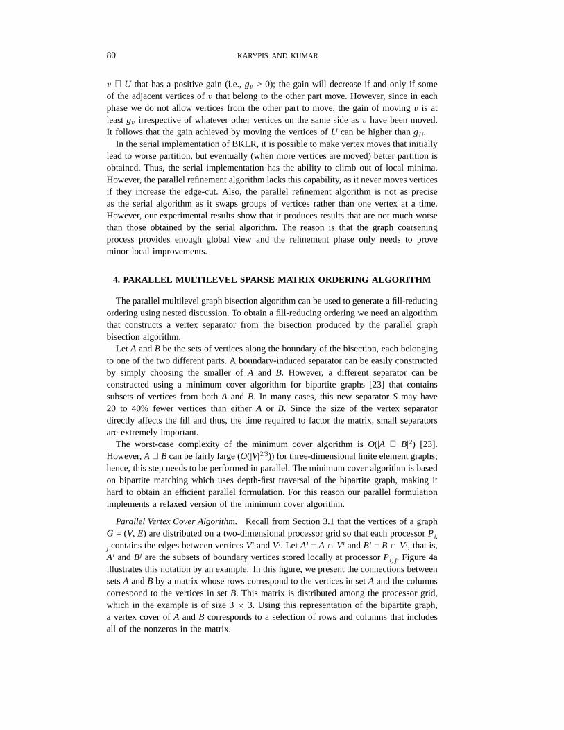
Parallel Vertex Cover Algorithm. Recall from Section 3.1 that the vertices of a graphG = (V, E) are distributed on a two-dimensional processor grid so that each processorPi,
j contains the edges between verticesVi andVj. Let Ai = A ∩ Vi andBj = B ∩ Vj, that is,Ai andBj are the subsets of boundary vertices stored locally at processorPi, j. Figure 4aillustrates this notation by an example. In this figure, we present the connections betweensetsA andB by a matrix whose rows correspond to the vertices in setA and the columnscorrespond to the vertices in setB. This matrix is distributed among the processor grid,which in the example is of size 3× 3. Using this representation of the bipartite graph,a vertex cover ofA andB corresponds to a selection of rows and columns that includesall of the nonzeros in the matrix.

PARALLEL ALGORITHM FOR GRAPH PARTITIONING 81
Each processorPi, j finds locally the minimum cover of edges betweenAi andBj. LetAi, j
c ⊆ Ai and Bi , jc ⊆ B j be such thatAi , j
c ∪ Bi, jc is this minimum cover. Figure 4b
shows the minimum covers computed by each processor. For example, the minimumcover computed by processorP0, 0 contains the vertices {a0, a1, b1}, that is A0, 0
c =
FIG. 4. An example of the computations performed while computing a minimal vertex cover in parallel:(a) original bipartite graph, (b) after local covers have been found, (c) union of the column covers, (d) afterlocally removing some of the row cover, (e) union of the row covers, and (f) after removing column covers.
82 KARYPIS AND KUMAR
{ a0, a1} and B0, 0c = { b1}. Note that the union ofAi , j
c and Bi, jc over all the processors
is a cover for all the edges betweenA andB. This cover can be potentially smaller thaneitherA or B. However, this cover is necessarily minimal, as it may contain vertices fromA (or B) such that the edges covered by them are also covered by other vertices in thecover. This can happen because the minimum cover for the edge-set at each processorPi, j is computed independently of the other processors. For example, the union of thelocal covers computed by all the processors in Fig. 4b is
{a0, a2, a3, a6, a7, a9, a11, a12, a13, a15, b1, b3, b4, b7, b8, b10, b14, b15},
which is not minimal, since for example we can removea3 and still have a vertex cover.The size of this cover can be potentially reduced as follows.
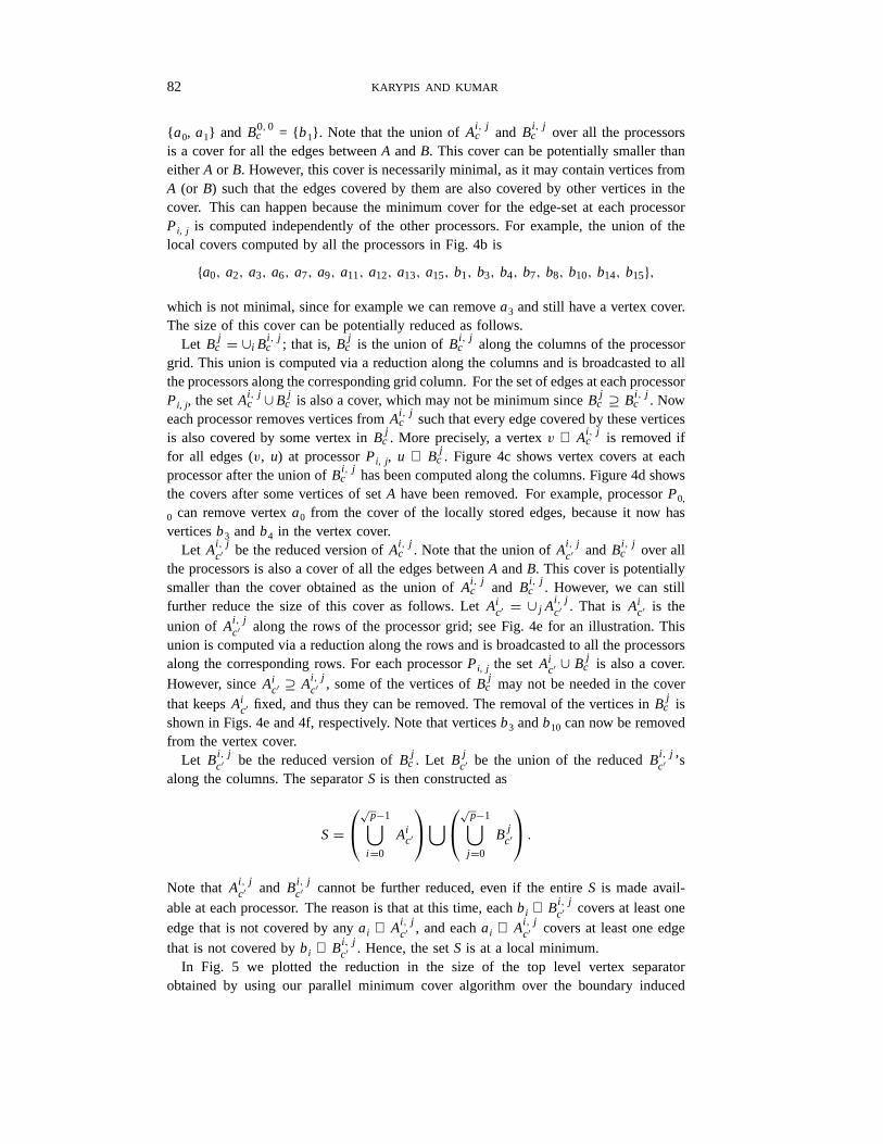
Let B jc = ∪i Bi , j
c ; that is, B jc is the union ofBi, j
c along the columns of the processorgrid. This union is computed via a reduction along the columns and is broadcasted to allthe processors along the corresponding grid column. For the set of edges at each processorPi, j, the setAi, j
c ∪B jc is also a cover, which may not be minimum sinceB j
c ⊇ Bi , jc . Now
each processor removes vertices fromAi , jc such that every edge covered by these vertices
is also covered by some vertex inB jc . More precisely, a vertexv ∈ Ai , j
c is removed iffor all edges (v, u) at processorPi, j, u ∈ B j
c . Figure 4c shows vertex covers at eachprocessor after the union ofBi, j
c has been computed along the columns. Figure 4d showsthe covers after some vertices of setA have been removed. For example, processorP0,
0 can remove vertexa0 from the cover of the locally stored edges, because it now hasverticesb3 andb4 in the vertex cover.
Let Ai, jc′ be the reduced version ofAi , j
c . Note that the union ofAi , jc′ and Bi , j
c over allthe processors is also a cover of all the edges betweenA andB. This cover is potentiallysmaller than the cover obtained as the union ofAi , j
c and Bi, jc . However, we can still
further reduce the size of this cover as follows. LetAic′ = ∪ j Ai , j
c′ . That is Aic′ is the
union of Ai , jc′ along the rows of the processor grid; see Fig. 4e for an illustration. This
union is computed via a reduction along the rows and is broadcasted to all the processorsalong the corresponding rows. For each processorPi, j the setAi
c′ ∪ B jc is also a cover.
However, sinceAic′ ⊇ Ai , j
c′ , some of the vertices ofB jc may not be needed in the cover
that keepsAic′ fixed, and thus they can be removed. The removal of the vertices inB j
c isshown in Figs. 4e and 4f, respectively. Note that verticesb3 andb10 can now be removedfrom the vertex cover.
Let Bi , jc′ be the reduced version ofB j
c . Let B jc′ be the union of the reducedBi , j
c′ ’salong the columns. The separatorS is then constructed as
S=√p−1⋃
i=0
Aic′
⋃√p−1⋃j=0
B jc′
.Note that Ai , j
c′ and Bi, jc′ cannot be further reduced, even if the entireS is made avail-
able at each processor. The reason is that at this time, eachbi ∈ Bi, jc′ covers at least one
edge that is not covered by anyai ∈ Ai, jc′ , and eachai ∈ Ai , j
c′ covers at least one edge
that is not covered bybi ∈ Bi, jc′ . Hence, the setS is at a local minimum.
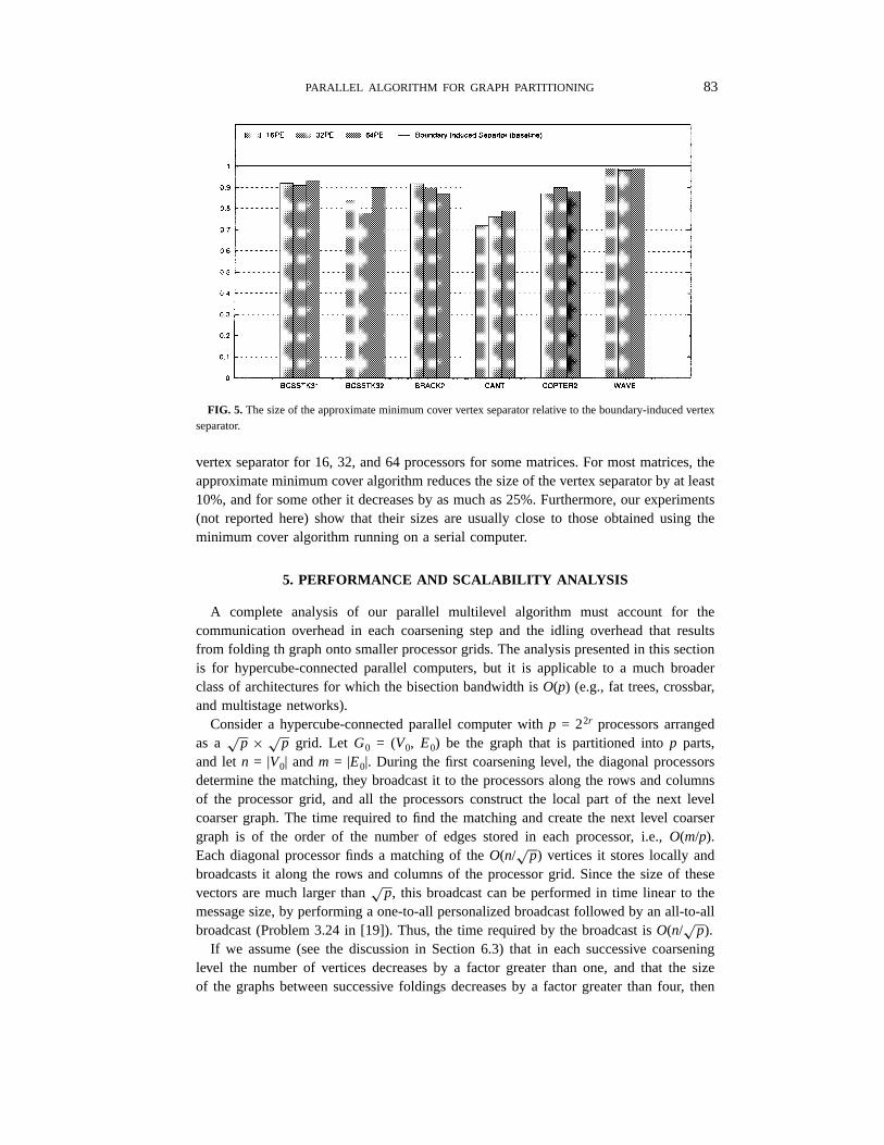
In Fig. 5 we plotted the reduction in the size of the top level vertex separatorobtained by using our parallel minimum cover algorithm over the boundary induced
PARALLEL ALGORITHM FOR GRAPH PARTITIONING 83
FIG. 5. The size of the approximate minimum cover vertex separator relative to the boundary-induced vertexseparator.
vertex separator for 16, 32, and 64 processors for some matrices. For most matrices, theapproximate minimum cover algorithm reduces the size of the vertex separator by at least10%, and for some other it decreases by as much as 25%. Furthermore, our experiments(not reported here) show that their sizes are usually close to those obtained using theminimum cover algorithm running on a serial computer.
5. PERFORMANCE AND SCALABILITY ANALYSIS
A complete analysis of our parallel multilevel algorithm must account for thecommunication overhead in each coarsening step and the idling overhead that resultsfrom folding th graph onto smaller processor grids. The analysis presented in this sectionis for hypercube-connected parallel computers, but it is applicable to a much broaderclass of architectures for which the bisection bandwidth isO(p) (e.g., fat trees, crossbar,and multistage networks).
Consider a hypercube-connected parallel computer withp = 22r processors arrangedas a√
p × √p grid. Let G0 = (V0, E0) be the graph that is partitioned intop parts,and letn = |V0| andm = |E0|. During the first coarsening level, the diagonal processorsdetermine the matching, they broadcast it to the processors along the rows and columnsof the processor grid, and all the processors construct the local part of the next levelcoarser graph. The time required to find the matching and create the next level coarsergraph is of the order of the number of edges stored in each processor, i.e.,O(m/p).Each diagonal processor finds a matching of theO(n/
√p) vertices it stores locally and
broadcasts it along the rows and columns of the processor grid. Since the size of thesevectors are much larger than
√p, this broadcast can be performed in time linear to the
message size, by performing a one-to-all personalized broadcast followed by an all-to-allbroadcast (Problem 3.24 in [19]). Thus, the time required by the broadcast isO(n/
√p).
If we assume (see the discussion in Section 6.3) that in each successive coarseninglevel the number of vertices decreases by a factor greater than one, and that the sizeof the graphs between successive foldings decreases by a factor greater than four, then

84 KARYPIS AND KUMAR
the amount of time required to compute a bisection is dominated by the time requiredto create the first level coarse graph. Thus, the time required to compute a bisection ofgraphG0 is
Tbissection= O
(m
p
)+ O
(n√p
). (1)
After finding a bisection, the graph is split and the task of finding a bisection foreach of these subgraphs is assigned to a different half of the processors. The amountof communciation required during this graph splitting is proportional to the number ofedges stored in each processor; thus, this time isO(m/p), which is of the same order asthe communication time required during the bisection step. This processes of bisectionand graph splitting continues for a total of logp times. At this time a subgraph is storedlocally on a single processor and thep-way partition of the graph has been found. Thetime required to compute the bisection of a subgraph at leveli is
Tbissectioni =O
(m/2i
p/2i
)+ O
(n/2i√p/2i
)
=O
(m
p
)+ O
(n√p
),
the same for all levels. Thus, the overall run time of the parallelp-way partitioning al-gorithm is
T parti t ion =(
O
(m
p
)+ O
(n√p
))log p
=O
(n log p√
p
). (2)
Equation (2) shows that asymptotically only a speedup ofO(√
p) can be achieved in thealgorithm. However, as our experiments in Section 6 show, higher speedup can be ob-tained. This is because the constant hidden in front ofO(m/p) is often much higher thanthat hidden in front ofO(n/
√p) particularly for 3D finite element graphs. Nevertheless,
from Eq. (2) we have that the partitioning algorithm is asymptotically unscalable. Thatis, it is not possible to obtain constant efficiency on increasingly large number of pro-cessors even if the problem size (O(n)) is increased arbitrarily.
However, a linear system solver that uses this parallel multilevel partitioning algorithmto obtain a fill reducing ordering prior to Cholesky factorization is not unscalable. Thisis because the time spent in ordering is considerably smaller than the time spent inCholesky factorization. The sequential complexity of Cholesky factorization of matricesarising in 2D and 3D finite elements applications isO(n1.5) andO(n2), respectively. Thecommunication overhead of parallel ordering over allp processors isO(n
√p log p),
which can be subsumed by the serial complexity of Cholesky factorization providednis large enough relative top. In particular, the isoefficiency [19] for 2D finite elementgraphs isO(p1.5 log3 p), and for 3D finite element graphs it isO(p log2 p). We haverecently developed a highly parallel sparse direct factorization algorithm [9, 17]. Theisoefficiency of this algorithm isO(p1.5) for both 2D and 3D finite element graphs.Thus, for 3D problems, the parallel ordering does not affect the overall scalability of theordering–factorization algorithm.

PARALLEL ALGORITHM FOR GRAPH PARTITIONING 85
TABLE 1
Various Matrices Used in Evaluating the Multilevel Graph Partitioning
and Sparse Matrix Ordering Algorithm
Matrix name Number of vertices Number of edges Description
4ELT 15606 45878 2D finite-element mesh
BCSSTK31 35588 572914 3D stiffness matrix
BCSSTK32 44609 985046 3D stiffness matrix
BRACK2 62631 366559 3D finite-element mesh
CANT 54195 1960797 3D stiffness matrix
COPTER2 55476 352238 3D finite-element mesh
CYLINDER93 45594 1786726 3D stiffness matrix
ROTOR 99617 662431 3D finite-element mesh
SHELL93 181200 2313765 3D stiffness matrix
WAVE 156317 1059331 3D finite-element mesh
6. EXPERIMENTAL RESULTS
We evaluated the performance of the parallel multilevel graph partitioning andsparse matrix ordering algorithm on a wide range of matrices arising in finite elementapplications. The characteristics of these matrices are described in Table 1.
We implemented our parallel multilevel algorithm on a 128-processor Cray T3Dparallel computer. Each processor on the T3D is a 150 MHz Dec Alpha chip. Theprocessors are interconnected via a three-dimensional torus network that has a peakunidirectional bandwidth of 150 Bytes per second and a small latency. We used SHMEMmessage passing library for communication. In our experimental setup, we obtained apeak bandwidth of 90 MBytes and an effective startup time of 4µs.
Since each processor on the T3D has only 64 MBytes of memory, some of the largermatrices could not be partitioned on a single processor. For this reason, we comparethe parallel run time on the T3D with the run time of the serial multilevel algorithmrunning on a SGI Challenge with 1.2 GBytes of memory and 150 MHz Mips R4400chip. Even though R4400 has a peak integer performance that is 10% lower than theAlpha, due to the significantly higher amount of secondary cache available on the SGImachine (1 Mbyte on SGI versus 0 Mbytes on T3D processors), the code running on asingle processor T3D is about 15% slower than that running on the SGI. The computedspeedups in the rest of this section are scaled to take this into account.4 All times reportedare in seconds. Since our multilevel algorithm uses randomization in the coarsening step,we performed all experiments with a fixed seed.
4The speedup is computed as 1.15× TSGI/TT3D, whereTSGI and TT3D are the run times on SGI and T3D,respectively.
86 KARYPIS AND KUMAR
6.1. Graph Partitioning
The performance of the parallel multilevel algorithm for the matrices in Table 1 is
shown in Table 2 for ap-way partition onp processors, wherep is 16, 32, 64, and
128. The performance of the serial multilevel algorithm for the same set of matrices
running on an SGI is shown in Table 3. For both the parallel and the serial multilevel
algorithm, the edge-cut and the run time are shown in the corresponding tables. In the
rest of this section, we will first compare the quality of the partitions produced by the
parallel multilevel algorithm, and then the speedup obtained by the parallel algorithm.
Figure 6 shows the size of the edge-cut of the parallel multilevel algorithm compared
to the serial multilevel algorithm. Any bars above the baseline indicate that the parallel
algorithm produces partitions with higher edge-cut than the serial algorithm. From this
graph we can see that for most matrices, the edge-cut of the parallel algorithm is worse
than that of the serial algorithm. This is due to the fact that the coarsening and refinement
performed by the parallel algorithm are less powerful. But in most cases, the difference
in edge-cut is quite small. For nine out of the ten matrices, the edge-cut of the parallel
algorithm is within 10% of that of the serial algorithm. Furthermore, the difference in
quality decreases as the number of partitions increases. The only exception is 4ELT,
for which the edge-cut of the parallel 16-way partition is about 27% worse than the
serial partition. However, even for this problem, when larger partitions are considered,
the relative difference in the edge-cut decreases; and for the 128-way partition, parallel
multilevel does slightly better than the serial multilevel algorithm.
Figure 7 shows the size of the edge-cut of the parallel algorithm compared to the
Multilevel Spectral Bisection algorithm (MSB) [3]. The MSB algorithm is a widely used
algorithm that has been found to generate high quality partitions with small edge-cuts.
We used the Chaco [11] graph partitioning package to produce the MSB partitions. As
before, any bars above the baseline indicate that the parallel algorithm generates partitions
with higher edge-cuts. From this figure we see that the quality of the parallel algorithm is
almost never worse than that of the MSB algorithm. For eight out of the ten matrices, the
parallel algorithm generated partitions with fewer edge-cuts, up to 50% better in some
cases. On the other hand, for the matrices that the parallel algorithm performed worse, it
is only by a small factor (less than 6%). This figure (along with Fig. 6) also indicates that
our serial multilevel algorithm outperforms the MSB algorithm. An extensive comparison
between our serial multilevel algorithm and MSB can be found in [16].
Tables 2 and 3 also show the run time of the parallel algorithm and the serial algorithm,
respectively. A number of conclusions can be drawn from these results. First, asp
increases, the time required for thep-way partition onp-processors decreases. Depending
on the size and characteristics of the matrix this decrease is quite substantial. The decrease
in the parallel run time is not linear with respect to the increase inp but somewhat smaller
for the following reasons: (a) Asp increases, the time required to perform thep-way
partition also increases; (there are more partitions to perform). (b) The parallel multilevel
algorithm incurs communication and idling overhead that limits the asymptotic speedup
to O(√
p) unless a good partition of the graph is available even before the partitioning
process starts (Section 5).
PA
RA
LLEL
ALG
OR
ITH
MF
OR
GR
AP
HP
AR
TIT
ION
ING
87
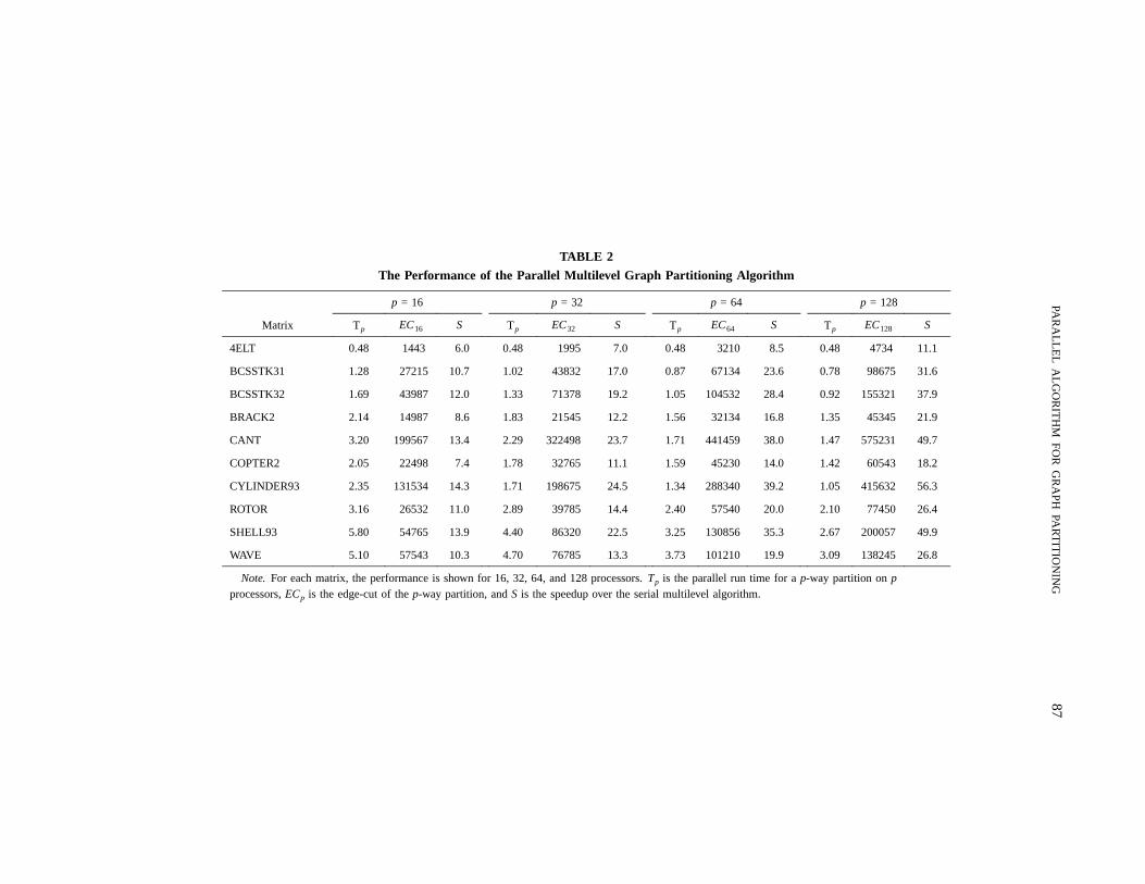
TABLE 2
The Performance of the Parallel Multilevel Graph Partitioning Algorithm
p = 16 p = 32 p = 64 p = 128
Matrix Tp EC16 S Tp EC32 S Tp EC64 S Tp EC128 S
4ELT 0.48 1443 6.0 0.48 1995 7.0 0.48 3210 8.5 0.48 4734 11.1
BCSSTK31 1.28 27215 10.7 1.02 43832 17.0 0.87 67134 23.6 0.78 98675 31.6
BCSSTK32 1.69 43987 12.0 1.33 71378 19.2 1.05 104532 28.4 0.92 155321 37.9
BRACK2 2.14 14987 8.6 1.83 21545 12.2 1.56 32134 16.8 1.35 45345 21.9
CANT 3.20 199567 13.4 2.29 322498 23.7 1.71 441459 38.0 1.47 575231 49.7
COPTER2 2.05 22498 7.4 1.78 32765 11.1 1.59 45230 14.0 1.42 60543 18.2
CYLINDER93 2.35 131534 14.3 1.71 198675 24.5 1.34 288340 39.2 1.05 415632 56.3
ROTOR 3.16 26532 11.0 2.89 39785 14.4 2.40 57540 20.0 2.10 77450 26.4
SHELL93 5.80 54765 13.9 4.40 86320 22.5 3.25 130856 35.3 2.67 200057 49.9
WAVE 5.10 57543 10.3 4.70 76785 13.3 3.73 101210 19.9 3.09 138245 26.8
Note. For each matrix, the performance is shown for 16, 32, 64, and 128 processors.Tp is the parallel run time for ap-way partition onp
processors,ECp is the edge-cut of thep-way partition, andS is the speedup over the serial multilevel algorithm.

88 KARYPIS AND KUMAR
TABLE 3
The Performance of the Serial Multilevel Graph Partitioning Algorithm
on an SGI, for 16-, 32-, 64-, and 128-way Partition
Matrix T16 EC16 T32 EC32 T64 EC64 T128 EC128
4ELT 2.49 1141 2.91 1836 3.55 2965 4.62 4600
BCSSTK31 11.96 25831 15.08 42305 17.82 65249 21.40 97819
BCSSTK32 17.62 43740 22.21 70454 25.92 106440 30.29 152081
BRACK2 16.02 14679 19.48 21065 22.78 29983 25.72 42625
CANT 37.32 199395 47.22 319186 56.53 442398 63.50 574853
COPTER2 13.22 21992 17.14 31364 19.30 43721 22.50 58809
CYLINDER93 29.21 126232 36.48 195532 45.68 289639 51.39 416190
ROTOR 30.13 24515 36.09 37100 41.83 53228 48.13 75010
SHELL93 69.97 51687 86.23 81384 99.65 124836 115.86 185323
WAVE 45.75 51300 54.37 71339 64.44 97978 71.98 129785
Note. Tp is the run time for ap-way partition, andECp is the edge-cut of thep-way partition.
We constructed Fig. 8 to compare the decrease in the parallel run time against variousideal situations. In this figure, we plotted the decrease in the run time forp equal to 32,64, and 128, relative to the run time ofp = 16 for some representative matrices fromTable 1. On the same graph, we also plotted the decrease in the run time if the speeduphad beenO(p), O(
√p), and O(log p), respectively. From Section 5, we know that the
asymptotic speedup obtained by the parallel multilevel algorithm is bounded byO(√
p).Also, from Section 3, we know that if only the parallelism due to the recursive stepis exploited, then the speedup of the parallel algorithm is bounded byO(log p). From
FIG. 6. Quality (size of the edge-cut) of our parallel multilevel algorithm relative to the serial multilevelalgorithm.
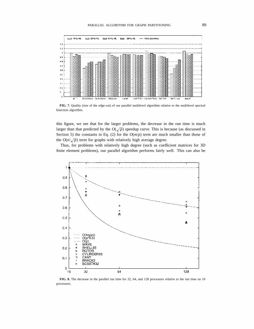
PARALLEL ALGORITHM FOR GRAPH PARTITIONING 89
FIG. 7. Quality (size of the edge-cut) of our parallel multilevel algorithm relative to the multilevel spectralbisection algorithm.
this figure, we see that for the larger problems, the decrease in the run time is muchlarger than that predicted by theO(
√p) speedup curve. This is because (as discussed in
Section 5) the constants in Eq. (2) for theO(m/p) term are much smaller than those ofthe O(n/
√p) term for graphs with relatively high average degree.
Thus, for problems with relatively high degree (such as coefficient matrices for 3Dfinite element problems), our parallel algorithm performs fairly well. This can also be
FIG. 8. The decrease in the parallel run time for 32, 64, and 128 processors relative to the run time on 16processors.
90 KARYPIS AND KUMAR
seen by looking at the speedup achieved by the parallel algorithm shown in Table 2. Wesee that for most such problems, speedup in the range of 14 to 25 was achieved on 32processors, and in the range of 22 to 56 on 128 processors. Since the serial multilevelalgorithm is quite fast (much faster than MSB), these speedups lead to a significantreduction in the time required to perform the partition. For most problems in our test set,it takes no more than 2 s to obtain a 128-partition on 128 processors. However, for theproblems with small average degrees, the decrease is very close toO(
√p) is predicted
by our analysis. The only exception is 4ELT, for which the speedup is close toO(log p).We suspect it is because the problem is too small, as even on a serial computer 128-waypartition takes less than 5 s.
6.2. Sparse Matrix Ordering
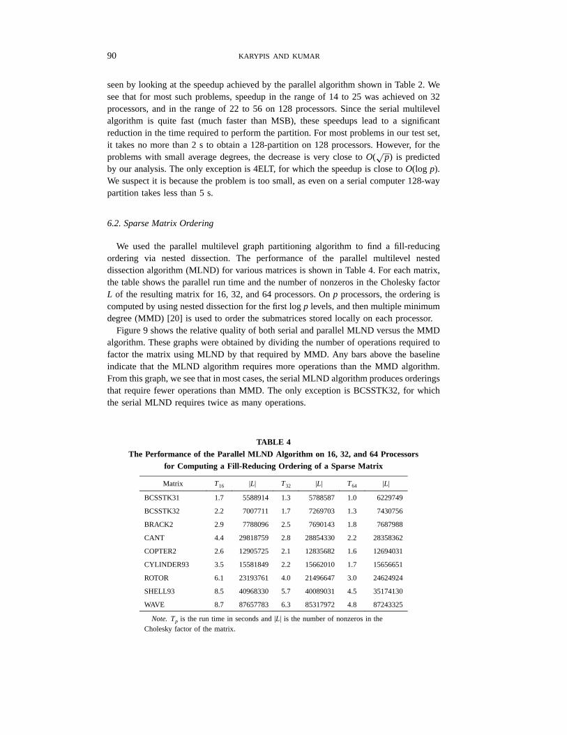
We used the parallel multilevel graph partitioning algorithm to find a fill-reducingordering via nested dissection. The performance of the parallel multilevel nesteddissection algorithm (MLND) for various matrices is shown in Table 4. For each matrix,the table shows the parallel run time and the number of nonzeros in the Cholesky factorL of the resulting matrix for 16, 32, and 64 processors. Onp processors, the ordering iscomputed by using nested dissection for the first logp levels, and then multiple minimumdegree (MMD) [20] is used to order the submatrices stored locally on each processor.
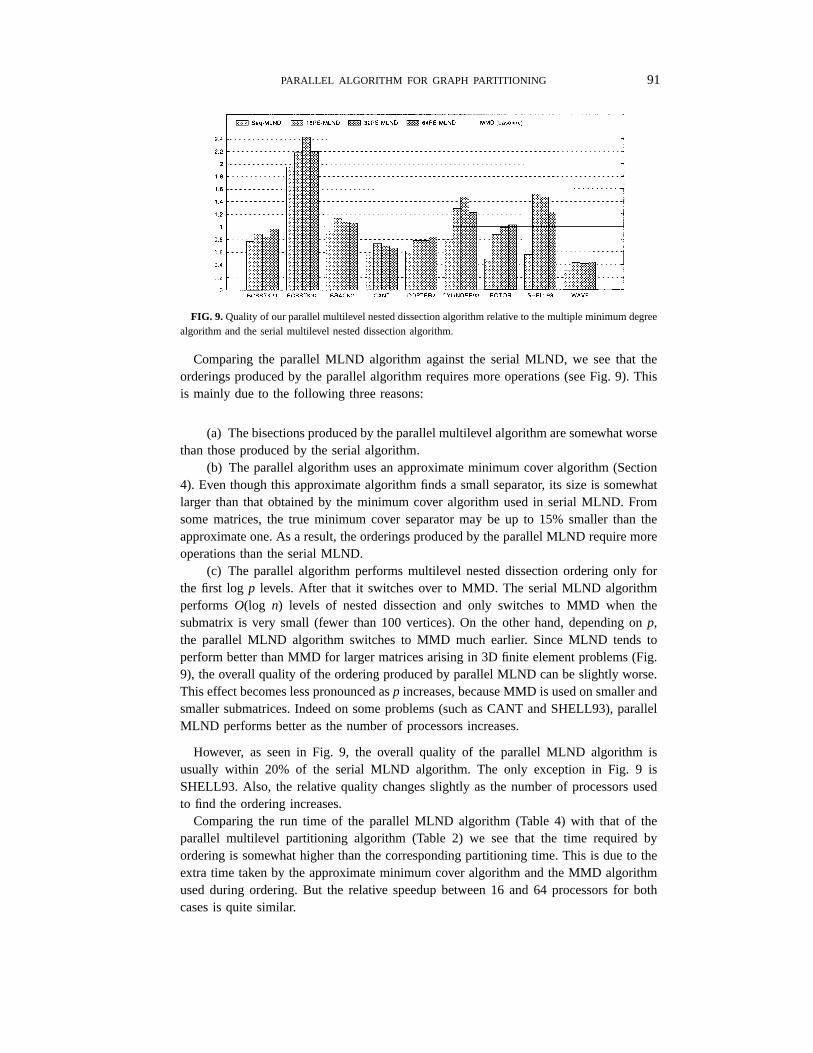
Figure 9 shows the relative quality of both serial and parallel MLND versus the MMDalgorithm. These graphs were obtained by dividing the number of operations required tofactor the matrix using MLND by that required by MMD. Any bars above the baselineindicate that the MLND algorithm requires more operations than the MMD algorithm.From this graph, we see that in most cases, the serial MLND algorithm produces orderingsthat require fewer operations than MMD. The only exception is BCSSTK32, for whichthe serial MLND requires twice as many operations.
TABLE 4
The Performance of the Parallel MLND Algorithm on 16, 32, and 64 Processorsfor Computing a Fill-Reducing Ordering of a Sparse Matrix
Matrix T16 |L| T32 |L| T64 |L|
BCSSTK31 1.7 5588914 1.3 5788587 1.0 6229749
BCSSTK32 2.2 7007711 1.7 7269703 1.3 7430756
BRACK2 2.9 7788096 2.5 7690143 1.8 7687988
CANT 4.4 29818759 2.8 28854330 2.2 28358362
COPTER2 2.6 12905725 2.1 12835682 1.6 12694031
CYLINDER93 3.5 15581849 2.2 15662010 1.7 15656651
ROTOR 6.1 23193761 4.0 21496647 3.0 24624924
SHELL93 8.5 40968330 5.7 40089031 4.5 35174130
WAVE 8.7 87657783 6.3 85317972 4.8 87243325
Note. Tp is the run time in seconds and |L| is the number of nonzeros in theCholesky factor of the matrix.
PARALLEL ALGORITHM FOR GRAPH PARTITIONING 91
FIG. 9. Quality of our parallel multilevel nested dissection algorithm relative to the multiple minimum degreealgorithm and the serial multilevel nested dissection algorithm.
Comparing the parallel MLND algorithm against the serial MLND, we see that theorderings produced by the parallel algorithm requires more operations (see Fig. 9). Thisis mainly due to the following three reasons:
(a) The bisections produced by the parallel multilevel algorithm are somewhat worsethan those produced by the serial algorithm.
(b) The parallel algorithm uses an approximate minimum cover algorithm (Section4). Even though this approximate algorithm finds a small separator, its size is somewhatlarger than that obtained by the minimum cover algorithm used in serial MLND. Fromsome matrices, the true minimum cover separator may be up to 15% smaller than theapproximate one. As a result, the orderings produced by the parallel MLND require moreoperations than the serial MLND.
(c) The parallel algorithm performs multilevel nested dissection ordering only forthe first logp levels. After that it switches over to MMD. The serial MLND algorithmperforms O(log n) levels of nested dissection and only switches to MMD when thesubmatrix is very small (fewer than 100 vertices). On the other hand, depending onp,the parallel MLND algorithm switches to MMD much earlier. Since MLND tends toperform better than MMD for larger matrices arising in 3D finite element problems (Fig.9), the overall quality of the ordering produced by parallel MLND can be slightly worse.This effect becomes less pronounced asp increases, because MMD is used on smaller andsmaller submatrices. Indeed on some problems (such as CANT and SHELL93), parallelMLND performs better as the number of processors increases.
However, as seen in Fig. 9, the overall quality of the parallel MLND algorithm isusually within 20% of the serial MLND algorithm. The only exception in Fig. 9 isSHELL93. Also, the relative quality changes slightly as the number of processors usedto find the ordering increases.
Comparing the run time of the parallel MLND algorithm (Table 4) with that of theparallel multilevel partitioning algorithm (Table 2) we see that the time required byordering is somewhat higher than the corresponding partitioning time. This is due to theextra time taken by the approximate minimum cover algorithm and the MMD algorithmused during ordering. But the relative speedup between 16 and 64 processors for bothcases is quite similar.

92 KARYPIS AND KUMAR
6.3. How Good Is the Diagonal Coarsening?
The analysis presented in Section 5 assumed that the size of the graph (i.e., the numberof edges) decreases by a factor greater than four before successive foldings. The amountof coarsening that can take place depends on the number of edges stored locally oneach diagonal processor. If this number is very small, then maximal independent subsetsfound by each diagonal processor will be very small. Furthermore, the next level coarsergraph will have even a smaller number of edges, since (a) edges in the matching areremoved, and (b) some of the edges of the matched vertices are common and thus arecollapsed together. On the other hand, if the average degree of a vertex is fairly high, thensignificant coarsening can be performed before folding. To illustrate the relation betweenthe average degree of a graph and the amount of coarsening that can be performed forthe first bisection, we performed a number of experiments on 16 and 64 processors. InTable 5 we show the reduction in the number of vertices and edges between foldings.
TABLE 5
The Reduction in the Number of Vertices and Edges between Successive Graph Foldings
4 × 4 2× 2 1× 1
Graph p V E V E V E
CANT 16 74.34 241.95 1.72 2.26
d = 72 64 16.71 39.09 2.63 3.51 1.78 2.20
BCSSTK31 16 49.23 118.57 1.90 2.50
d = 44 64 8.67 29.06 2.67 2.99 2.60 3.20
BCSSTK32 16 16.04 32.55 2.67 3.73
d = 32 64 4.99 7.43 2.94 3.40 1.98 2.33
BRACK2 16 7.43 7.06 2.48 3.14
d = 12 64 6.84 6.41 1.83 1.93 1.82 2.06
ROTOR 16 12.31 12.60 1.90 2.06
d = 12 64 5.07 4.77 2.47 2.70 1.85 1.99
COPTER2 16 7.61 7.64 1.89 2.04
d = 12 64 2.77 2.59 1.96 1.92 2.62 3.02
4ELT 16 2.01 2.04 4.48 5.76
d = 6 64 1.30 1.31 1.72 1.76 4.19 5.50
Note. For each graph, the columns labeled withV(E) give the factor by which the number of vertices(edges) is reduced between successive foldings. These results are shown for three processor grids, 4× 4,2 × 2, and 1× 1, that correspond to the quadrant of the grid to which the graph was folded. For example,for BCSSTK32, when 64 processors are used, the number of vertices was reduced by a factor of 4.99before being folded to 16 processors (4× 4 grid). For the same graph, the number of vertices was reducedfurther by a factor of 2.94 before being folded to 4 processors, and by another 1.98 factor before beingfolded down to a single processor. Thus, the graph that a single processor receives has 4.99× 2.94× 1.98= 16.65 times fewer vertices than the original graph. Under each graph, the average degreed of the graphis shown.
PARALLEL ALGORITHM FOR GRAPH PARTITIONING 93
A number of interesting conclusions can be drawn from this table. For graphs withrelatively high average degree (e.g., CANT, BCSSTK31, BCSSTK32), most of thecoarsening is performed on the entire processor grid. For instance, on 64 processors,for CANT, the average degree of a vertex on the diagonal processors is 72/8 = 9. As aresult significant coarsening can be performed before the edges of the diagonal processorsget depleted. By the time the parallel multilevel algorithm is forced to perform a folding,both the number of vertices and the number of edges have decreased by a large factor. Inmany cases, this factor is substantially higher than that required by the analysis. For mostof these graphs, over 90% of the overall computation of coarsening is performed using allthe processors, and only a small fraction is performed by smaller processor grids. Thistype of graphs corresponds to the coefficient matrices of 3D finite element problemswith multiple degrees of freedom that are widely used in scientific and engineeringapplications. From this, we can see that the diagonal coarsening can easily be scaled upto 256 or even 1024 processors for graphs with average degree higher than 25 or 40,respectively.
For low-degree graphs (e.g., BRACK2, COPTER2, and ROTOR) with average degreeof 12 or less, the number of vertices decreases by a smaller factor than the high degreegraphs. For BRACK2, for each vertex, each diagonal processor has on the average 12/8= 1.5 vertices; thus, only a limited amount of coarsening can be performed. Note that for4ELT, the number of vertices and the number of edges decrease only by a small factor,which explains the poor speedup obtained for this problem.
7. CONCLUSION
In this paper we presented a parallel formulation of multilevel recursive bisectionalgorithm for partitioning a graph and for producing a fill-reducing order via nesteddissection. Our experiments show that our parallel algorithms are able to produce goodpartitions and orderings for a wide range of problems. Furthermore, our algorithmsachieve a speedup of up to 56 on 128-processor Cray T3D.
Due to the two-dimensional mapping scheme used in the parallel formulation, itsasymptotic speedup is limited toO(
√p) because the matching operation is performed
only on the diagonal processors. In contrast, for one-dimensional mapping scheme usedin [1, 14, 24] the asymptotic speedup can beO(p) for large enough graphs. However,this two-dimensional mapping has the following advantages. First, the actual speedupon graphs with large average degrees is quite good as shown in Fig. 8. The reason isthat for these graphs, the formation of the next level coarser graph (which is completelyparallel with two-dimensional mapping) dominates the computation of the matching.Second, the two-dimensional mapping requires fewer communication operations (onlybroadcast and reduction operations along the rows and columns of the processor grid) ineach coarsening step compared with one-dimensional mapping. Hence on machines withslow communication network (high message startup time and/or small communicationbandwidth), the two-dimensional mapping can provide better performance even for graphswith small degree. Third, the two-dimensional mapping is central to the parallelization ofthe minimal vertex cover computation presented in Section 4. It is unclear if the algorithmfor computing minimal vertex cover of a bipartite graph can be efficiently parallelizedwith one-dimensional mapping.
94 KARYPIS AND KUMAR
The parallel graph partitioning and sparse matrix reordering algorithms described in thispaper are available in the PARMETIS graph partitioning library that is publicly availableon WWW at http://www.cs.umn.edu/∼metis.
REFERENCES
1. S. T. Barnard, Pmrsb: Parallel multilevel recursive spectral bisection,in “Supercomputing 1995.”
2. S. T. Barnard and H. Simon, A parallel implementation of multilevel recursive spectral bisection forapplication to adaptive unstructured meshes,in “Proceedings of the Seventh SIAM Conference on ParallelProcessing for Scientific Computing,” pp. 627–632, 1995.
3. S. T. Barnard and H. D. Simon, A fast multilevel implementation of recursive spectral bisection forpartitioning unstructured problems,in “Proceedings of the Sixth SIAM Conference on Parallel Processingfor Scientific Computing,” pp. 711–718, 1993.
4. T. Bui and C. Jones, A heuristic for reducing fill in sparse matrix factorization,in “6th SIAM Conf.Parallel Processing for Scientific Computing,” pp. 445–452, 1993.
5. P. Diniz, S. Plimpton, B. Henrickson, and R. Leland, Parallel algorithms for dynamically partitioningunstructured grids,in “Proceedings of the Seventh SIAM Conference on Parallel Processing for ScientificComputing,” pp. 615–620, 1995.
6. C. M. Fiduccia and R. M. Mattheyses, A linear time heuristic for improving network partitions,in “Proc.19th IEEE Design Automation Conference,” pp. 175–181, 1982.
7. J. Garbers, H. J. Promel, and A. Steger, Finding clusters in VLSI circuits,in “Proceedings of IEEEInternational Conference on Computer Aided Design,” pp. 520–523, 1990.
8. A. George and J. W.-H. Liu, “Computer Solution of Large Sparse Positive Definite Systems,” Prentice-Hall, Englewood Cliffs, NJ, 1981.
9. A. Gupta, G. Karypis, and V. Kumar, Highly scalable parallel algorithms for sparse matrix factorization,IEEE Trans. Parallel Distrib. Systems8, 5 (May 1997), 502–520. [Available on WWW at URL http://www.cs.umn.edu/∼karypis]
10. M. T. Heath, E. G.-Y. Ng, and B. W. Peyton, Parallel algorithms for sparse linear systems,SIAM Rev.
33 (1991), 420–460. [Also appears in “Parallel Algorithms for Matrix Computations,” (K. A. Gallivanet al., Eds.), SIAM, Philadelphia, PA, 1990]
11. B. Hendrickson and R. Leland, “The Chaco User’s Guide,” version 1.0, Technical Report SAND93-2339,Sandia National Laboratories, 1993.
12. B. Hendrickson and R. Leland, “A Multilevel Algorithm for Partitioning Graphs,” Technical ReportSAND93-1301, Sandia National Laboratories, 1993.
13. G. Karypis and V. Kumar, “Analysis of Multilevel Graph Partitioning,” Technical Report TR 95-037,Department of Computer Science, University of Minnesota, 1995. [Also available on WWW at URLhttp://www.cs.umn.edu/∼karypis] [A short version appears in “Supercomputing ’95”]
14. G. Karypis and V. Kumar, “Parallel Multilevelk-way Partitioning Scheme for Irregular Graphs,” TechnicalReport TR 96-036, Department of Computer Science, University of Minnesota, 1996. [Also available onWWW at URL http://www.cs.umn.edu/∼karypis] [A short version appears in “Supercomputing ’96”]
15. G. Karypis and V. Kumar, Multilevelk-way partitioning scheme for irregular graphs,J. Parallel Distrib.Comput.48, No. 1 (1998), 96–129.
16. G. Karypis and V. Kumar, A fast and highly quality multilevel scheme for partitioning irregular graphs,SIAM J. Sci. Comput.,to appear. [Also available on WWW at URL http://www.cs.umn.edu/∼karypis] [Ashort version appears in “Intl. Conf. on Parallel Processing 1995”]
17. G. Karypis and V. Kumar, “Fast Space Cholesky Factorization on Scalable Parallel Computers,” Technicalreport, Department of Computer Science, University of Minnesota, Minneapolis, MN, 1994. [A shortversion appears in the “Eighth Symposium on the Frontiers of Massively Parallel Computation,” 1995][Available on WWW at URL http://www.cs.umn.edu/∼karypis]
18. B. W. Kernighan and S. Lin, An efficient heuristic procedure for partitioning graphs,Bell Syst. Tech. J.
1970.

PARALLEL ALGORITHM FOR GRAPH PARTITIONING 95
19. V. Kumar, A. Grama, A. Gupta, and G. Karypis, “Introduction to Parallel Computing: Design andAnalysis of Algorithms,” Benjamin/Cummings Publishing Company, Redwood City, CA, 1994.
20. J. W.-H. Liu, Modification of the minimum degree algorithm by multiple elimination,ACM Trans. Math.Software11 (1985), 141–153.
21. M. Luby, A simple parallel algorithm for the maximal independent set problem,SIAM J. Comput.15, 4(1986), 1036–1053.
22. R. Ponnusamy, N. Mansour, A. Choudhary, and G. C. Fox, Graph contraction and physical optimizationmethods: A quality–cost tradeoff for mapping data on parallel computers,in “International Conferenceof Supercomputing,” 1993.
23. A. Pothen and C.-J. Fan, Computing the block triangular form of a sparse matrix,ACM Trans. Math.
Software1990.
24. P. Raghavan, “Parallel Ordering Using Edge Contraction,” Technical Report CS-95-293, Department ofComputer Science, University of Tennessee, 1995.
25. E. Rothberg, Performance of panel and block approaches to sparse Cholesky factorization on the iPSC/860 and Paragon multicomputers,in “Proceedings of the 1994 Scalable High Performance ComputingConference,” May 1994.
26. J. E. Savage and M. G. Wloka, Parallelism in graph partitioning,J. Parallel Distrib. Compt.13 (1991),257–272.
27. H. D. Simon and S.-H. Teng, “How Good is Recursive Bisection?,” Technical Report RNR-93-012, NASSystems Division, Moffet Field, CA, 1993.
GEORGE KARYPIS received his Ph.D. in computer science at the University of Minnesota, and he iscurrently an assistant professor at the Department of Computer Science and Engineering at the University ofMinnesota. His research interests span the areas of parallel algorithm design, applications of parallel processingin scientific computing and optimization, sparse matrix computations, parallel programming languages andlibraries, and data mining. His recent work has been in the areas of parallel sparse direct solvers, serial andparallel graph partitioning algorithms, parallel matrix ordering algorithms, and scalable parallel preconditioners.His research has resulted in the development of software libraries for unstructured mesh partitioning (METISand ParMETIS) and for parallel Cholesky factorization (PSPASES). He is the author of over 20 research articlesand a coauthor of the widely used textbook “Introduction to Parallel Computing.”
VIPIN KUMAR received his Ph.D. in computer science at the University of Maryland, and he is currently aprofessor at the Department of Computer Science and Engineering at the University of Minnesota. His currentresearch interests include parallel computing, parallel algorithms for scientific computing problems, and datamining. His research has resulted in the development of highly efficient parallel algorithms and software forsparse matrix factorization (PSPASES), graph partitioning (METIS and ParMETIS), and dense hierarchicalsolvers. Kumar’s research in performance analysis resulted in the development of the isoefficiency metric foranalyzing the scalability of parallel algorithms. He is the author of over 100 research articles and a coauthorof the widely used textbook “Introduction to Parallel Computing.” Kumar has given over 50 invited talksat various conferences, workshops, and national labs and has served as chair/co-chair for many conferences/workshops in the area of parallel computing. Kumar serves on the editorial boards ofIEEE Parallel andDistributed Technology, IEEE Transactions of Data and Knowledge Engineering, Parallel Computing, and theJournal of Parallel and Distributed Computing. He is a senior member of IEEE and a member of SIAMand ACM.
Received November 1, 1996; revised October 15, 1997; accepted October 20, 1997